Hapi: A Multivariable Land-Surface Transformer for Medium-Range Hydrological Forecasting at Continental Scale
Abstract
Accurate flood forecasts several days in advance are essential for flood control, water-resource management, and emergency response. Producing them at high resolution over a continental domain calls for local hydrological detail together with spatial context extending from river basins to synoptic weather systems. We developed Hapi, a U-Net Swin Transformer that uses fine three-dimensional patches and hierarchical shifted-window attention to forecast discharge, surface runoff, snow water equivalent, and soil wetness across the contiguous United States. The model produces 24–72-hour forecasts at resolution, with learned Laplacian task weights adjusting each variable’s contribution to training. On 2024 test data using reconstructed weather and land-surface inputs from ERA5-Land, Hapi outperformed an operational physics-based model and a state-of-the-art AI model in flood detection. Independent validation against 3,881 U.S. Geological Survey gauges and a Hurricane Helene case study supported its advantage over the physics-based model in reproducing daily discharge. Controlled experiments showed that learned task weighting strengthens rare-flood detection, which is particularly sensitive to changes in precipitation inputs. Hapi produced a four-variable, 72-hour forecast across the contiguous United States with an average inference time of 0.11 seconds on a single A100 GPU.
Keywords: deep learning, hydrological forecasting, flood detection, land-surface modeling, Swin Transformer, continental-scale forecasting
1 Introduction
Accurate flood forecasts several days in advance are essential for flood control, water-resource management, and emergency response (Tellman et al., 2021; Alfieri et al., 2013). A central challenge is to produce these forecasts at high resolution over continental domains while representing local hydrological variation and basin-to-synoptic-scale context. Operational systems address this challenge with process-based simulators. The Global Flood Awareness System (GloFAS) (Alfieri et al., 2013), and the U.S. National Water Model (Cosgrove et al., 2024), for example, solve land-surface and river-routing equations at continental scale and produce a full land-surface state. Their ensembles consume millions of CPU-hours per year, depend on hand-tuned regional parameters, and take months to adapt to new variables or regions.

Deep learning provides a complementary approach, but most hydrological applications have represented rivers as collections of individual basins or gauges. Within this setting, long short-term memory networks (LSTMs), are widely used to predict streamflow (Nearing et al., 2021). A single model trained across many catchments can outperform individually calibrated process models when conditioned on basin attributes (Kratzert et al., 2019; Newman et al., 2015; Addor et al., 2017). This approach now spans multiple timescales, global regionalization, and operational flood warning (Gauch et al., 2021; Beck et al., 2020; Nearing et al., 2024; Nevo et al., 2022). Caravan (Kratzert et al., 2023) and NeuralHydrology (Kratzert et al., 2022) support standardized development and evaluation of these basin-based models. Transformers and time-series foundation models have also been applied to 120-h streamflow prediction and zero-shot forecasting at unseen stations (Demiray and Demir, 2026; Sun and Sun, 2026). Despite their broader reach, these models produce basin or gauge sequences without explicit spatial interaction across a gridded domain.
Gridded models extend deep-learning discharge prediction beyond this pointwise representation. RiverMamba (Shams Eddin et al., 2025) brings spatial context to global discharge forecasting and outperforms an operational LSTM baseline, particularly beyond 48 h. SwinFlood (Song et al., 2025) combines a convolutional neural network with Swin Transformer blocks within a single urban–rural catchment on the Shenzhen River. These models extend hydrological deep learning from independent basin sequences to spatially distributed discharge forecasts.
Related developments in weather and Earth-system forecasting offer strategies for handling the spatial and multivariable dimensions of this problem. Hierarchical and graph-based models build broad spatial context without applying global attention to every grid point (Bi et al., 2023; Lam et al., 2023; Chen et al., 2023; Nguyen et al., 2024). Generalist Earth-system models forecast heterogeneous fields through shared architectures (Bodnar et al., 2025; Nguyen et al., 2023; Schmude et al., 2024; Vaughan et al., 2025). Similarly, ecLand emulators show that several prognostic land-surface states can be advanced together (Wesselkamp et al., 2025). A complementary line of hydrological research encodes conservation or process structure through mass-conserving recurrent networks, differentiable process models, or differentiable routing (Hoedt et al., 2021; Feng et al., 2022; Bindas et al., 2024). Together, these studies provide ingredients for spatial or multivariable prediction, but they do not jointly establish high-resolution continental forecasting of multiple hydrological states, threshold-based flood skill, independent gauge validation, and computationally efficient inference in one model.
To address this gap, we introduce Hapi, a hierarchical transformer that forecasts river discharge, surface runoff, snow water equivalent, and soil wetness over the contiguous United States (CONUS) out to 72 h while representing local hydrological variation and basin-to-synoptic-scale context. Figure 1 shows an example of Hapi’s 72-h discharge forecast across CONUS. Hapi combines fine three-dimensional patches, which retain local detail, with hierarchical shifted-window attention that expands spatial context without global attention over the full grid. Learned task weights account for the different scales and distributions of the four targets. During autoregressive rollout, the four predicted fields feed into the next step, while meteorological forcing is updated externally. On a 2024 CONUS holdout, we evaluate reanalysis-conditioned flood detection and continuous discharge skill against persistence, the operational GloFAS forecast, and RiverMamba. ERA5-Land fields supply the meteorological forcing in this experiment, isolating hydrological-state prediction from errors in numerical weather prediction (NWP); a precipitation-perturbation experiment probes sensitivity to departures from this forcing. Our contributions are
- •
A hierarchical vision architecture for continental hydrology. Hapi preserves the two-dimensional grid, uses fine three-dimensional convolutional patches to limit early spatial aggregation, and expands context through hierarchical Swin V2 stages, as described in Section 3. A mirrored decoder and multiscale skip connections then reconstruct fine spatial structure while the hierarchy builds broader meteorological context within one continental model.
- •
Automatic balancing of heterogeneous hydrological targets. Hapi forecasts discharge, runoff, snow water equivalent, and soil wetness without manually tuning their relative loss weights, despite their different scales and error distributions, as described in Section 3.3. Under matched training conditions, learned task weighting improves discharge accuracy and flood-detection skill relative to uniform or fixed weighting, with the largest gains at rarer thresholds, as shown in Section 4.5.
- •
Leading flood detection with independent observational validation. Hapi achieves the highest flood-detection F1 in 20 of 21 lead–threshold comparisons in Section 4.2, including every threshold from 1.5 to 100 yr at 48 and 72 h. All 21 F1 advantages over RiverMamba remain significant after multiplicity correction, as shown in Appendix N. Hapi also has the highest base-rate-invariant symmetric extremal dependence index, SEDI, in 18 of 21 comparisons with GloFAS and persistence in Appendix O. Against 3,881 U.S. Geological Survey gauges, hereafter USGS gauges, Hapi also achieves higher median Nash–Sutcliffe efficiency, NSE, than GloFAS and persistence at every lead, as shown in Section 4.3.
2 Data
We use a daily gridded dataset assembled from GloFAS reanalysis (Harrigan et al., 2020), ERA5-Land (Copernicus Climate Change Service, 2019), and static terrain and upstream drainage fields. The dataset spans twenty years, 2005–2024, over CONUS on a latitude–longitude grid, approximately 5 km, at a 24-h time step. ERA5-Land data are regridded from their native resolution to the GloFAS grid. The GloFAS grid consists of cells. Ocean cells and cells outside CONUS are zero-padded to preserve the rectangular grid shape and masked out when computing the loss and evaluation metrics, leaving 416,298 active land cells, as described in Appendix B.
2.1 Variables
Each sample from the dataset contains 12 input variables grouped by their role in the autoregressive rollout described in Section 3. Table 1 lists their sources, units, and definitions.
| Role | Source | Variables and units |
|---|---|---|
| Prognostic | GloFAS reanalysis | River discharge, m3 s-1; runoff water equivalent, mm; snow water equivalent, mm; soil wetness index, dimensionless |
| Forcing | ERA5-Land | Total runoff, ro, m; precipitation, tp, m; evaporation, e, m; soil water in layer 1, swvl1, m3 m-3; solar radiation, ssrd, J m-2; 2 m air temperature, t2m, K |
| Static | DEM; GloFAS v4.0 | Surface elevation, m; upstream drainage area, m2 |
ERA5-Land supplies the six forcing variables at each rollout step, making the prediction of hydrological states reanalysis-conditioned. The two runoff variables differ because GloFAS runoff is routed and prognostic, whereas ERA5-Land ro is an unrouted forcing. Similarly, swvl1 describes the top 7 cm, while the prognostic soil wetness index aggregates the top three layers with vegetation-dependent weights. Appendix A reports the variable-specific normalization choices and the distributions that motivate them.
2.2 Data Splits
We follow the WeatherBench convention and split the data by calendar year. Models are trained on 2005–2022, comprising eighteen years and approximately 6,575 daily samples, while the 365 samples from 2023 are used only for validation. The held-out test set covers the first ten months of 2024, from 2024-01-01 through 2024-11-01, after accounting for the history buffer at the start of the window. It is used only for the results in Section 4. The three calendar ranges are disjoint and ordered in time.
2.3 Flood Detection Thresholds
For flood detection, we use the per-cell return levels distributed as the GloFAS v4.0 auxiliary data to define flood events (ECMWF, 2023). GloFAS derives these fields by fitting a Gumbel distribution, the member of the generalized extreme value family, to annual maxima using L-moments. The annual maxima come from LISFLOOD (Burek et al., 2013) physical simulations forced with ERA5 in the GloFAS reanalysis (Harrigan et al., 2020) for 1979–2022. The fitted distributions provide return levels for 1.5, 2, 5, 10, 20, 50, 100, 200, and 500 years. At each grid cell , the -year return level is the discharge threshold satisfying , where is the annual maximum discharge. Thus, a 100-year return level has a 1% chance of being exceeded in any given year, and exceedances can occur in consecutive years. Using these published fields keeps the event definition consistent with the one used by GloFAS for flood warnings. The fitting window ends in 2022, before the 2024 test window, so the thresholds carry no information from the validation or test periods.
The return-level fields align exactly with our grid, allowing us to select a CONUS subset without interpolation, as described in Appendix B. Cells that are undefined in the source fields are excluded, leaving valid cells within the -cell CONUS land mask.
For each return period , a cell is labeled as flooded when the discharge exceeds the -year threshold. The corresponding predicted flood mask is obtained by applying the same return level to the model’s predicted discharge.
3 Method
Hapi is a U-Net Swin Transformer V2 for gridded multivariable hydrology at resolution. Its backbone integrates a U-Net (Ronneberger et al., 2015) encoder–decoder, Swin Transformer V2 blocks (Liu et al., 2022), 2D rotary position embeddings (Su et al., 2024; Fang et al., 2024), and gated attention (Qiu et al., 2025). We also use learned per-variable Laplacian task weighting in place of the hand-tuned weights used by prior multivariable forecasters, together with multi-step fine-tuning at a randomized rollout depth for the four prognostic land-surface variables. Given historical frames of input variables on an grid, the model predicts prognostic variables at the next time step, as shown in Figure 2.
Existing gridded Earth-system forecasters take different architectural routes, which typically suit the atmosphere better than the land surface. RiverMamba (Shams Eddin et al., 2025) traverses the grid as a 1D sequence with bidirectional Mamba blocks (Gu and Dao, 2024), committing to a serial scan order on a 2D field. Pangu-Weather (Bi et al., 2023) adds a 3D Earth-specific transformer with an explicit pressure-level axis, matched to atmospheric vertical structure but unnatural for surface-only variables. GraphCast (Lam et al., 2023) uses a multi-mesh icosahedral graph that trades resolution uniformity for global coverage. FuXi (Chen et al., 2023) and Aurora (Bodnar et al., 2025) use U-shaped vision transformers similar to our backbone but designed for atmospheric targets. We use the Swin hierarchy because its multiscale windows span river-channel to synoptic scales. Hapi retains a two-dimensional hierarchy and reconstructs full-resolution outputs through a mirrored decoder and skip connections.
Hapi also differs from existing models in its token representation. Strategies include per-variable tokenization with cross-attention (Nguyen et al., 2023), physically grouped branches (Bi et al., 2023), and variable-agnostic latent encoders (Jaegle et al., 2022; Bodnar et al., 2025). Hapi keeps a monolithic patch embedding but distinguishes prognostic, forcing, and static inputs at the rollout level, a separation described in Section 3.2. The hydrological targets span six orders of magnitude, and up to 78% of their values are exactly zero, as shown in Table 12, making uniform standardization unsuitable. We combine per-variable log1p reparameterization with learnable Laplacian task weighting in Section 3.3, adapting the likelihood-based weighting form of Kendall et al. (2018) to a mean absolute error (MAE), objective for heavy-tailed hydrological targets. For autoregressive rollout, AI weather models stabilize long horizons with curriculum fine-tuning (Lam et al., 2023), randomized forecast intervals (Nguyen et al., 2024), or diffusion-based forecasting (Price et al., 2025; Hatanpää et al., 2025); we fine-tune on rollouts of randomized depth, in the manner of Brandstetter et al. (2022).
3.1 Architecture
To limit early aggregation of local hydrological variation, Hapi uses small spatial patches with . A three-dimensional convolutional (Conv3D) layer, with kernel and stride maps the input tensor to tokens of dimension , where is the batch size. This projection combines the variables and historical frames within each patch, leaving a two-dimensional token grid for subsequent attention.
Hapi builds spatial context through stages of Swin Transformer blocks to reduce attention costs. Attention operates within local windows, and shifted windows allow information to pass across window boundaries. Between stages, patch merging halves each spatial dimension and doubles the channel width. This encoder expands the area covered by each window while reducing the number of tokens at the next stage.
The decoder mirrors the encoder’s structure by upsampling through patch unmerging, which uses a learned linear expansion and pixel-shuffle rearrangement to double each spatial dimension. Skip connections concatenate encoder and decoder features at corresponding resolutions, giving the decoder direct access to encoder representations that bypass the bottleneck. A final linear projection produces channels at the original resolution, one predicted field per prognostic variable.

Position encoding.
Within an attention window, token interactions depend on relative spatial position as well as the local features. Swin V2 represents position through a learned multilayer perceptron (MLP), that maps coordinate offsets to an additive attention bias. We use axial 2D rotary position embeddings (RoPE) (Su et al., 2024; Heo et al., 2024), to encode these offsets directly in the query–key interaction without learning a position-bias network. For each attention head of dimension , we group vector components into even–odd pairs and alternate row and column rotations across successive pairs. For a query vector at window position , the rotation is
| (1) |
where the angles are defined by
| (2) |
with indexing the frequency bands. The coordinates and index the row and column within each attention window. Applying the same rotations to key vectors makes the query–key dot product depend on position through relative row and column offsets. We set for the windows.
Gated attention.
A Swin window can contain river channels, dry land, and ocean cells, so the relevance of neighboring information can vary across locations and features. Within each head, standard softmax attention uses one normalized set of weights to mix all features of the value vectors. Consequently, it passes a mixture of values forward, even when none provides useful information for a particular feature of the receiving token. We add separate, query-dependent control using the element-wise sigmoid gate of Qiu et al. (2025), computed from the receiving token and applied after attention. The gate allows each token to attenuate individual attended features before the output projection. For input token features within a window, we compute the gate logits together with the query, key, and value projections:
| (3) |
The gated attention output is
| (4) |
where is the sigmoid function and denotes element-wise multiplication. The gate assigns a scale between zero and one to each feature in every token and attention head.
3.2 Autoregressive Rollout with Prognostic–Forcing Separation
The model rolls out by feeding its output back as input. Variables update by different rules at each step: prognostic variables, comprising river discharge, runoff, snow water equivalent, and soil wetness index, are replaced by their predicted fields; forcing variables, including precipitation, temperature, and radiation, are supplied from ERA5-Land; static descriptors, comprising elevation and upstream drainage area, stay fixed. This separates the prognostic hydrological state from meteorological forcing: forecast products can supply the forcing fields, while terrain remains fixed at every step. Prognostic predictions are held within declared physical ranges before they are fed back: the nonnegative variables are snapped to the point mass at zero in their target distributions, and the soil wetness index is clipped to , as described in Appendix C. The rule is applied only at intermediate steps and is identical during training and inference; the loss at the final step is computed from the raw output. Section 3.3 describes the training schedule for multi-step fine-tuning at a randomized rollout depth.
3.3 Training Objective
Foundation models such as Pangu-Weather (Bi et al., 2023), GraphCast (Lam et al., 2023), FuXi (Chen et al., 2023), and GenCast (Price et al., 2025) balance per-variable losses with hand-tuned scalar weights. RiverMamba also fixes its severity and lead-time weights by hand (Shams Eddin et al., 2025), although its single target does not require cross-variable balancing. We adapt the likelihood-based Gaussian task weighting of Kendall et al. (2018), which uses mean squared error, to a Laplacian form with MAE for hydrology’s heavy-tailed targets with frequent zeros. Per-variable log-scales are learned end to end. Loss is computed only on the prognostic outputs, so .
Heavy-tailed targets, comprising discharge, snow water equivalent, and runoff, are reparameterized with so that rare large values do not dominate the loss, as described in Appendix A. For a prediction and target , define the residual in normalized space. The masked mean absolute error for variable is
| (5) |
where is the per-variable validity mask of Appendix B, so zero-padded ocean and out-of-domain cells neither contribute to the numerator nor inflate the denominator.
Each variable has a learnable log-scale . Writing for a scalar residual of variable , the Gaussian formulation of Kendall et al. (2018) gives the negative log-likelihood up to an additive constant, with denoting the log-standard deviation. For our MAE objective, we use a zero-centered Laplacian residual model with scale :
| (6) |
Averaging its negative log-likelihood over valid cells and the batch, and dropping the constant , gives . Averaging over variables yields
| (7) |
where is the inverse Laplace scale and serves as the learned task weight. Increasing reduces this weight, and the additive term prevents all weights from collapsing to zero. For fixed , stationarity with respect to gives . The learned weights therefore balance the variables according to their error scales, removing the need to tune their relative loss weights by hand. The are global task-level scales shared across samples, locations, and lead times. They adapt the relative contributions of the four prognostic variables during optimization; they are not input-dependent predictive uncertainties and do not provide calibrated forecast intervals. The implementation also admits fixed per-variable prior weights multiplying each term; they are uniform in every run reported here, and Appendix F gives the converged .
Multi-step fine-tuning follows Brandstetter et al. (2022) by randomizing the rollout horizon. At each iteration, we sample , autoregressively roll out the model for steps, and evaluate the loss on the prediction at step :
| (8) |
The intermediate predictions are fed back into the model without detaching the computational graph, so gradients from propagate through the complete -step rollout. We use .
3.4 Model Configuration
The final model uses two consecutive daily frames, , of 12 input variables to predict the next-day fields of four prognostic variables. Longer histories produced only marginal accuracy gains at greater computational cost. Although the temporal projection can be reconfigured for any history length, provided the best accuracy–efficiency trade-off among those tested.
The encoder comprises three stages with Swin blocks and uses embedding dimension , patch size , and window size . The decoder mirrors this stage structure. The complete model has 43.96 million parameters. In a Bayesian search over these four hyperparameters, shallow encoders with fine tokenization achieved the lowest validation losses. The selected configuration follows this pattern, as shown in Appendix E.
Training begins with single-step pretraining and continues with randomized multi-step fine-tuning using . We optimize the task log-scales during pretraining and freeze them during fine-tuning. Freezing the scales prevents them from compensating for accumulated rollout error, leaving the model parameters to reduce that error, as described in Appendix D. Appendix F gives the full training details and learned log-scales.
4 Results
We evaluated Hapi from overall forecast skill to specific capabilities and limitations. We first compared discharge forecasts with persistence, GloFAS, and RiverMamba at continental and gauge scales. We then examined the contributions of multivariable prediction and learned task weighting, evaluated the other prognostic variables, and tested variation across river subsets and perturbed meteorological forcing. Finally, we used Hurricane Helene to illustrate event-scale behavior and assessed computational performance.
4.1 Baselines, Metrics, and Statistical Analysis
We evaluated gridded discharge against GloFAS reanalysis using a common verification target and compared Hapi with persistence, the operational GloFAS forecast, and RiverMamba. The comparisons cover 24-, 48-, and 72-h leads during the 2024 test period. Flood-threshold detection is the primary outcome, complemented by continuous discharge metrics, per-cell analyses, and paired moving-block bootstrap inference. The verification target is the GloFAS reanalysis 24-h mean river discharge, the field Hapi is trained to predict in Section 2.1 and from which the per-cell return-level thresholds are derived in Section 2.3. Scores therefore measure agreement with that reanalysis, using an identical target for every model.
We compare Hapi against three baselines. Persistence carries forward the last discharge field observed at forecast issue time and holds it constant across all leads; the 72-h forecast therefore uses the field from three days before the target. The lag-1 autocorrelation of daily streamflow exceeds 0.95 on large catchments, making persistence a strong short-lead baseline. GloFAS forecast is the operational, physics-based global flood forecasting system of the Copernicus Emergency Management Service (Alfieri et al., 2013). The GloFAS v4 forecasts evaluated here are generated with the distributed hydrological model LISFLOOD OS (Burek et al., 2013). We use the Copernicus Emergency Management Service product cems-glofas-forecast, with system version operational, hydrological model LISFLOOD, the control_forecast member, and variable river_discharge_in_the_last_24_hours, at lead times of 24, 48, and 72 h, retrieved over the same CONUS box as the training grid. This operational forecast is evaluated against the same verification target as the other models.
RiverMamba (Shams Eddin et al., 2025) is a recent gridded deep-learning discharge forecaster at the same resolution. We follow its published issue-time convention: RiverMamba uses seven historical days through , issues at , and predicts through , without using a day- discharge nowcast. Thus the tabulated 24-, 48-, and 72-h leads follow each system’s stated forecast issue time, although RiverMamba’s latest discharge input is one day older than Hapi’s at the same nominal lead. Only Hapi and GloFAS carry the four prognostic land-surface variables; RiverMamba is discharge-only. RiverMamba was run on its native global domain for forecast evaluation, and its CONUS predictions were extracted for the comparisons below.
Each system is evaluated with its respective meteorological inputs. Hapi uses ERA5-Land forcing over the forecast horizon, whereas the operational GloFAS product uses its native forecast forcing. The Hapi–GloFAS comparison therefore measures reanalysis-conditioned Hapi skill against the archived operational product, not performance under identical meteorological inputs.
We exclude the U.S. National Water Model because its streamflow predictions are defined on NHDPlus river reaches rather than the regular grid used here (Cosgrove et al., 2024). A direct comparison would require a separately validated reach-to-grid mapping or an independent gauge evaluation that includes the National Water Model, both outside the scope of this study.
Continuous performance is evaluated using MAE and root mean squared error (RMSE), in m3 s-1, together with the dimensionless NSE and Kling–Gupta efficiency, KGE. The primary flood-detection analysis uses per-cell GloFAS v4.0 return levels at seven return periods from 1.5 to 100 yr and reports F1, precision, recall, and the critical success index (CSI). Exploratory results for the more uncertain 200- and 500-yr levels are reported in Appendix L. Definitions and aggregation conventions for all evaluation metrics are given in Appendix H. The primary discharge metrics use the 2024 test window at 24-, 48-, and 72-h leads on the CONUS land mask, which contains 414,795 valid cells after excluding 1,503 cells without defined return levels.
Threshold-crossing skill is the primary outcome, and continuous skill is secondary. The decision a flood forecast supports is binary: at a given return period, warn or do not warn. Threshold-based metrics directly quantify this decision, whereas continuous error statistics do not. A forecast can have low RMSE while misclassifying threshold exceedances during flood events. Unadjusted accuracy is uninformative at these base rates because a forecast with no warnings would score close to one. F1 balances missed events against false alarms without requiring a cost ratio, which depends on the application.
F1 depends on the event base rate, precluding direct comparison between values at different return-period thresholds, such as 1.5 and 100 yr. We use F1 to compare models at a fixed return period and the base-rate-invariant SEDI to compare skill across return periods, as described in Appendix O. Pooled continuous metrics characterize domain-wide performance and emphasize high-discharge rivers. We therefore also compute the metrics independently at each grid cell and summarize their spatial distributions in Appendix M.
Uncertainty in F1 and SEDI differences is estimated with a paired moving-block bootstrap using 30-day blocks and replicates, as described in Appendix N. Within each replicate, the same days are resampled for both models. Holm correction is applied across the 21 lead–return-period comparisons within each model pair and metric. Hapi–persistence and Hapi–GloFAS comparisons use 302 common dates per lead, whereas Hapi–RiverMamba comparisons use the 294 dates available for both models. We report paired differences with percentile intervals and multiplicity-adjusted decisions.
4.2 Discharge Forecast Skill
Hapi achieves the highest flood-detection F1 in 20 of the 21 lead–threshold comparisons in Table 2, including all seven thresholds from 1.5 to 100 yr at both 48 and 72 h. Hapi exceeds RiverMamba throughout and falls below persistence only at the 100-yr threshold at 24 h, by 0.0015. Figure 3a shows that Hapi’s margin over the strongest baseline is larger at 48 and 72 h than at 24 h across all seven thresholds. At the 1.5-yr and 100-yr thresholds shown in Figure 3b,c, Hapi has the lowest false-alarm ratio among the four models at every lead.
We next used the paired moving-block bootstrap described in Appendix N to quantify uncertainty in the F1 comparisons reported in Table 2. Hapi’s higher F1 than RiverMamba was significant after Holm–Bonferroni correction in all 21 lead–threshold comparisons. Against GloFAS, Hapi’s higher F1 remained significant at every threshold at 24 h. At the 5-yr threshold, the Hapi–GloFAS difference was at 24 h, with a 95% interval of –. The difference was at 72 h, with a 95% interval of –; both comparisons were significant after Holm–Bonferroni correction.
Among Hapi, GloFAS, and persistence, Hapi has the highest SEDI in 18 of 21 lead–threshold comparisons, including all seven at both 48 and 72 h. The SEDI analysis in Appendix O complements the fixed-threshold F1 comparisons by allowing skill to be compared across event rarity. At 72 h, Hapi’s SEDI decreases from 0.931 at the 1.5-yr threshold to 0.724 at the 100-yr threshold, indicating lower flood-detection skill at more extreme thresholds. Unlike F1, this decrease is not an automatic consequence of the lower event frequency.
In Table 3, Hapi has the lowest pooled MAE and RMSE at 24 h, but GloFAS leads on RMSE, NSE, and KGE at 48 and 72 h. At 48 h, Hapi and GloFAS have nearly identical MAE, both rounding to 2.94 m3/s; GloFAS has the lowest MAE at 72 h, while persistence has the highest KGE at 24 h. Pooling emphasizes high-discharge rivers in a domain spanning five orders of magnitude of discharge, motivating a separate evaluation at individual grid cells.
Although GloFAS has higher pooled NSE at 48 and 72 h, Hapi has higher median per-cell NSE at both leads in Table 4. Among Hapi, GloFAS, and persistence, Hapi has the highest median per-cell NSE at every lead: 0.902, 0.823, and 0.776, compared with 0.698, 0.637, and 0.559 for GloFAS. At 72 h, Hapi exceeds GloFAS at 79.2% of scored cells and persistence at 92.3%, with median NSE differences of and , respectively. These spatial comparisons show that Hapi’s NSE advantage extends across most scored cells despite its lower pooled NSE at longer leads.
| Return period, years | ||||||||
|---|---|---|---|---|---|---|---|---|
| Model | Lead | 1.5 | 2 | 5 | 10 | 20 | 50 | 100 |
| persistence | 24 h | 0.836 | 0.799 | 0.709 | 0.627 | 0.562 | 0.496 | 0.470 |
| GloFAS | 24 h | 0.773 | 0.718 | 0.584 | 0.473 | 0.396 | 0.306 | 0.264 |
| RiverMamba | 24 h | 0.728 | 0.660 | 0.479 | 0.347 | 0.259 | 0.187 | 0.145 |
| Hapi | 24 h | 0.885 | 0.863 | 0.786 | 0.700 | 0.612 | 0.524 | 0.468 |
| persistence | 48 h | 0.726 | 0.671 | 0.544 | 0.434 | 0.353 | 0.275 | 0.233 |
| GloFAS | 48 h | 0.747 | 0.685 | 0.535 | 0.413 | 0.333 | 0.239 | 0.191 |
| RiverMamba | 48 h | 0.697 | 0.622 | 0.433 | 0.301 | 0.212 | 0.138 | 0.098 |
| Hapi | 48 h | 0.833 | 0.799 | 0.691 | 0.569 | 0.460 | 0.337 | 0.269 |
| persistence | 72 h | 0.653 | 0.590 | 0.447 | 0.334 | 0.256 | 0.177 | 0.140 |
| GloFAS | 72 h | 0.720 | 0.653 | 0.493 | 0.365 | 0.277 | 0.184 | 0.134 |
| RiverMamba | 72 h | 0.592 | 0.566 | 0.381 | 0.252 | 0.171 | 0.103 | 0.071 |
| Hapi | 72 h | 0.800 | 0.760 | 0.638 | 0.502 | 0.391 | 0.263 | 0.208 |
| 24 h lead | 48 h lead | 72 h lead | ||||||||||
|---|---|---|---|---|---|---|---|---|---|---|---|---|
| Model | MAE | RMSE | NSE | KGE | MAE | RMSE | NSE | KGE | MAE | RMSE | NSE | KGE |
| persistence | 2.43 | 41.64 | 0.996 | 0.998 | 4.55 | 78.38 | 0.985 | 0.992 | 6.30 | 109.68 | 0.970 | 0.985 |
| GloFAS | 2.79 | 43.29 | 0.995 | 0.997 | 2.94 | 44.59 | 0.995 | 0.997 | 3.15 | 46.90 | 0.995 | 0.997 |
| RiverMamba | 2.11 | 35.67 | 0.997 | 0.997 | 3.05 | 54.53 | 0.993 | 0.993 | 3.80 | 70.46 | 0.988 | 0.986 |
| Hapi | 1.57 | 32.30 | 0.997 | 0.990 | 2.94 | 63.19 | 0.990 | 0.980 | 4.08 | 89.72 | 0.980 | 0.976 |
| Lead | Model | Median NSE | Median KGE | Median | Hapi wins vs. | |
|---|---|---|---|---|---|---|
| % cells | median NSE | |||||
| 24 h | Hapi | 0.902 | 0.891 | 0.973 | – | – |
| persistence | 0.823 | 0.911 | 1.000 | 89.4% | +0.054 | |
| GloFAS | 0.698 | 0.804 | 0.993 | 93.0% | +0.142 | |
| 48 h | Hapi | 0.823 | 0.832 | 0.967 | – | – |
| persistence | 0.560 | 0.779 | 1.000 | 91.5% | +0.217 | |
| GloFAS | 0.637 | 0.758 | 0.990 | 82.9% | +0.124 | |
| 72 h | Hapi | 0.776 | 0.795 | 0.962 | – | – |
| persistence | 0.339 | 0.669 | 1.000 | 92.3% | +0.363 | |
| GloFAS | 0.559 | 0.709 | 0.989 | 79.2% | +0.142 | |
4.3 Independent Validation Against USGS Gauges
The preceding grid-based comparisons use GloFAS reanalysis as the verification target. Against USGS daily discharge observations, Hapi also has the highest median NSE at every lead, exceeding GloFAS at about two-thirds of gauges with finite paired NSE values in Table 5. This comparison covers 3,881 gauges matched by drainage area to unique grid cells and retained with paired days during the 2024 test window. The matching and filtering protocol is given in Appendix I.
Hapi’s median NSE remains near 0.16 through 72 h, while that of persistence declines from 0.070 to . Its median percent bias is also smaller, ranging from to %, compared with to % for GloFAS and to % for persistence. Hapi thus retains its advantage in median NSE against an observational target, although the gauge and grid-cell samples differ.
This aggregate advantage coexists with substantial variation among gauges. At 24 h, Hapi’s median NSE is 0.160, with 10th and 90th percentiles of and 0.661; its lowest median NSE occurs in basins larger than 50,000 km2. Figure 4 illustrates this variation using gauges nearest the median Hapi 72-h NSE within each region and drainage-area band. The Missouri panels show missed seasonal peaks on the Two Medicine and Milk rivers and muted variability on the North Loup River. The South Atlantic–Gulf and Pacific Northwest panels generally track the observed variation more closely, though the Owyhee forecasts contain pulses with weak observational counterparts. These hydrographs show why a small median bias does not imply accurate discharge timing or magnitude at every gauge.
| Lead | Model | NSE | KGE | RMSE | PBIAS | ||
|---|---|---|---|---|---|---|---|
| median | median | m3/s | % | % | % | ||
| 24 h | Hapi | 0.160 | 0.310 | 19.4 | +1.2 | 59.7 | 23.2 |
| GloFAS | 0.076 | 0.273 | 20.6 | +4.8 | 54.7 | 20.9 | |
| persistence | 0.070 | 0.271 | 20.9 | +5.3 | 54.8 | 18.6 | |
| 48 h | Hapi | 0.165 | 0.312 | 19.3 | +0.5 | 59.7 | 23.4 |
| GloFAS | 0.064 | 0.271 | 20.8 | +4.7 | 54.4 | 20.0 | |
| persistence | -0.032 | 0.203 | 22.3 | +5.4 | 46.0 | 12.9 | |
| 72 h | Hapi | 0.159 | 0.306 | 19.4 | +0.7 | 59.6 | 23.2 |
| GloFAS | 0.041 | 0.264 | 21.2 | +4.3 | 53.2 | 18.3 | |
| persistence | -0.108 | 0.153 | 23.7 | +5.5 | 39.3 | 10.1 |
4.4 Four-Variable and Discharge-Only Model Comparison
We compare the available four-variable and discharge-only configurations at 24-h lead to characterize their discharge skill. The discharge-only configuration treats the other three land-surface variables as prescribed inputs and uses weighted MAE. Because the configurations also differ in training schedule, input-data revision, and loss formulation, this comparison cannot isolate the effect of multivariable prediction or its propagation during longer rollouts.
The four-variable configuration has lower MAE and RMSE, while leading flood-detection F1 at six of seven thresholds in Table 6. Discharge-only MAE is 32% higher, at 2.07 versus 1.57 m3/s, and RMSE is 27% higher, at 41.14 versus 32.30 m3/s. The discharge-only configuration nevertheless has higher KGE and 100-yr F1, so the advantage depends on the metric. The next comparison holds the four-variable configuration fixed to examine the contribution of loss weighting.
| F1 by GloFAS return period, yr | |||||||||||
|---|---|---|---|---|---|---|---|---|---|---|---|
| Variant | MAE | RMSE | NSE | KGE | 1.5 | 2 | 5 | 10 | 20 | 50 | 100 |
| Full Hapi | 1.57 | 32.30 | 0.997 | 0.990 | 0.885 | 0.863 | 0.786 | 0.700 | 0.612 | 0.524 | 0.468 |
| Discharge-only | 2.07 | 41.14 | 0.996 | 0.992 | 0.869 | 0.842 | 0.761 | 0.672 | 0.593 | 0.522 | 0.481 |
4.5 Loss-Weighting Ablation
To distinguish the effect of task scaling from the effect of adapting the scales during training, we compare three loss formulations with the same four-variable architecture, inputs, targets, data splits, batch size, and 16-GPU training budget. Uniform task weights minimize the unweighted mean of the four normalized-variable MAEs. Fixed task scales use the Laplacian objective in Equation 7, with the four log-scales set to the values learned by the adaptive control and held constant throughout training. Learned task scales use the same Laplacian objective but optimize the log-scales jointly with the model parameters. Table 7 compares the three single-step models at 24 h on the 2024 test window.
Learned task scales yield the lowest discharge errors and highest F1 at every threshold. Uniform weights increase MAE by 24%, from 1.59 to 1.97 m3/s, and reduce F1 by 4.7–11.5 percentage points, with the largest loss at the 100-yr threshold. Fixed scales bring MAE to 1.64 m3/s, only 3% above the learned-scale result, accounting for most of the improvement in this metric.
Learning the task scales reduces MAE only slightly relative to fixed scales but produces larger gains in F1 at rare-event thresholds. At the 100-yr threshold, fixed scales raise F1 from 0.345 to 0.382, whereas learning the scales raises it further to 0.460. The additional gain from learning the scales exceeds the gain from fixed scaling at every threshold from 10 to 100 yr, indicating that adaptation particularly benefits rare-flood detection.
| F1 by GloFAS return period, yr | |||||||||||
|---|---|---|---|---|---|---|---|---|---|---|---|
| Variant | MAE | RMSE | NSE | KGE | 1.5 | 2 | 5 | 10 | 20 | 50 | 100 |
| Learned task scales | 1.59 | 30.94 | 0.998 | 0.990 | 0.877 | 0.856 | 0.779 | 0.690 | 0.601 | 0.513 | 0.460 |
| Uniform task weights | 1.97 | 38.71 | 0.996 | 0.985 | 0.830 | 0.802 | 0.710 | 0.607 | 0.505 | 0.410 | 0.345 |
| Fixed task scales | 1.64 | 31.77 | 0.997 | 0.987 | 0.856 | 0.835 | 0.748 | 0.647 | 0.544 | 0.445 | 0.382 |
4.6 Non-Discharge Prognostic Skill
The preceding comparisons focus on discharge, one of Hapi’s four prognostic variables. We next evaluate the three other variables against persistence to assess their forecast skill beyond carrying the initial state forward. Against their reanalysis targets, Hapi predicts runoff and soil wetness with lower RMSE and MAE and higher NSE than persistence at all three leads in Table 8. Runoff NSE remains positive, from 0.328 at 24 h to 0.298 at 72 h, whereas carrying the initial runoff field forward gives negative NSE at every lead.
For soil wetness and screened snow, Hapi’s advantage becomes clearer at longer leads. Persistence is already accurate at 24 h for these slowly varying stores, but its RMSE increases more rapidly during the rollout. By 72 h, Hapi reduces RMSE relative to persistence by 36% for soil wetness and 32% for screened snow. Hapi also has lower MAE and higher NSE for both stores at every lead, while persistence retains higher 24-h KGE.
The snow comparison depends on three cells with persistent target snow accumulation among the 349,402 evaluated cells; these three cells are excluded by the screening rule in Appendix J. These cells contribute about 99% of Hapi’s unscreened squared error. Retaining them raises Hapi’s 24-h RMSE from 2.51 to 22.20 mm and gives persistence lower RMSE and higher NSE at every lead. Table 8 reports both masks, showing the improvement across the screened snow field alongside the concentrated errors that reverse the full-mask ranking.
| Variable | Lead | Model | RMSE | MAE | NSE | KGE |
| Runoff water equivalent, 418,792 cells | ||||||
| 24 h | Hapi | 1.8580 | 0.2850 | 0.3281 | ||
| persistence | 0.4156 | |||||
| 48 h | Hapi | 1.8900 | 0.2999 | 0.3107 | 0.3365 | |
| persistence | ||||||
| 72 h | Hapi | 1.9070 | 0.3105 | 0.2980 | 0.3327 | |
| persistence | ||||||
| Snow water equivalent, 349,402 cells | ||||||
| 24 h | Hapi | |||||
| persistence | 2.7350 | 0.5889 | 0.9988 | 0.9964 | ||
| 48 h | Hapi | 0.8476 | ||||
| persistence | 4.6310 | 0.9964 | 0.9925 | |||
| 72 h | Hapi | 1.0500 | ||||
| persistence | 6.2310 | 0.9935 | 0.9883 | |||
| screened, 349,399 cells | ||||||
| 24 h | Hapi | 2.5100 | 0.5692 | 0.9977 | ||
| persistence | 0.9961 | |||||
| 48 h | Hapi | 3.4610 | 0.8040 | 0.9956 | 0.9947 | |
| persistence | ||||||
| 72 h | Hapi | 4.2460 | 1.0010 | 0.9933 | 0.9941 | |
| persistence | ||||||
| Soil wetness index, 426,768 cells | ||||||
| 24 h | Hapi | 0.0091 | 0.0037 | 0.9980 | ||
| persistence | 0.9986 | |||||
| 48 h | Hapi | 0.0104 | 0.0045 | 0.9974 | 0.9969 | |
| persistence | ||||||
| 72 h | Hapi | 0.0122 | 0.0057 | 0.9965 | 0.9957 | |
| persistence | ||||||
4.7 Per-Subset Skill
For discharge, the continental F1 comparison combines rivers of different sizes and flood activity, leaving open whether Hapi’s advantage holds across the river network. We therefore compare Hapi and RiverMamba at their nominal forecast leads on AIFAS river points, flood-active cells, and three drainage-area groups separated at 500 and 5,000 km2. The first two subsets overlap the drainage groups; their definitions and cell counts are given in Appendix L. RiverMamba’s latest discharge input is one day older at each nominal lead, as described in Section 4.1.
Hapi has higher F1 in all 75 comparisons across five subsets, three leads, and the five thresholds from 1.5 to 20 yr. At the 2-yr threshold, the largest gaps occur in the small-river subset, where Hapi leads by 0.185–0.212 across the three leads in Table 9. The four exceptions within the full 1.5–100-yr comparison occur on large rivers at the 50- and 100-yr thresholds at 48 and 72 h. At 72 h, RiverMamba’s F1 is 0.187 versus Hapi’s 0.090 at 50 yr and 0.131 versus 0.013 at 100 yr. The broad advantage therefore weakens for rare exceedances on large rivers at longer leads.
Continuous discharge metrics test whether these spatial differences extend beyond threshold crossings. Hapi has lower MAE on every subset at 24 h and on three of the five subsets at every lead, as shown in Appendix L. On large rivers, RiverMamba has lower MAE from 48 h and higher NSE at 72 h, while its KGE is already higher at 24 h.
| 24 h | 48 h | 72 h | ||||
|---|---|---|---|---|---|---|
| Subset | Hapi | RM | Hapi | RM | Hapi | RM |
| AIFAS | 0.870 | 0.681 | 0.807 | 0.641 | 0.767 | 0.604 |
| Flood-active | 0.878 | 0.734 | 0.822 | 0.696 | 0.787 | 0.662 |
| Small rivers | 0.854 | 0.643 | 0.793 | 0.609 | 0.758 | 0.550 |
| Medium rivers | 0.902 | 0.727 | 0.838 | 0.677 | 0.794 | 0.636 |
| Large rivers | 0.891 | 0.781 | 0.792 | 0.707 | 0.717 | 0.666 |
4.8 Forcing-Perturbation Sensitivity
The preceding forecasts use ERA5-Land forcing, whereas operational predictions depend on uncertain weather forecasts. We therefore test how flood-detection skill responds when precipitation departs from reanalysis. We focus on precipitation because errors in rainfall amount directly alter the water input available for runoff generation and can shift discharge across flood thresholds. At rollout steps 2 and 3, precipitation is multiplied by , where is a standardized Gaussian field correlated in space and across rollout steps. This intervention preserves dry cells and scales the perturbation with rainfall intensity. We test , 0.2, 0.5, and 1.0; the 24-h forcing is unchanged, and the zero-amplitude run recovers the unperturbed baseline.
The log-normal multiplier changes both rainfall variability and mean amount. Its median is one, but its mean is , reaching about 1.65 at . The multiplier ranges corresponding to Gaussian perturbations within one standard deviation of zero are 0.82–1.22 at and 0.61–1.65 at , representing asymmetric multiplicative departures rather than symmetric percentage errors.
F1 and NSE decrease or remain unchanged across the four tested amplitudes, with larger relative F1 losses at rare thresholds. At 48 h and , NSE changes from 0.990 to 0.987, while 100-yr F1 falls from 0.269 to 0.039. At the intermediate amplitude , the 100-yr F1 loss is already 38%, compared with 4% at the 1.5-yr threshold. The small change in pooled NSE therefore conceals substantial sensitivity in rare-event detection. Because these perturbations are not calibrated to a weather forecast system, operational skill still requires evaluation with archived NWP forecasts.
| Log-noise amplitude | |||||
|---|---|---|---|---|---|
| Lead | Metric | 0.00 | 0.20 | 0.50 | 1.00 |
| 48 h | F1 @ 1.5-yr | 0.833 | 0.827 | 0.800 | 0.709 |
| F1 @ 5-yr | 0.691 | 0.677 | 0.602 | 0.357 | |
| F1 @ 20-yr | 0.460 | 0.442 | 0.334 | 0.114 | |
| F1 @ 100-yr | 0.269 | 0.254 | 0.168 | 0.039 | |
| NSE | 0.990 | 0.990 | 0.990 | 0.987 | |
| 72 h | F1 @ 1.5-yr | 0.800 | 0.789 | 0.743 | 0.609 |
| F1 @ 5-yr | 0.638 | 0.616 | 0.507 | 0.244 | |
| F1 @ 20-yr | 0.391 | 0.367 | 0.244 | 0.066 | |
| F1 @ 100-yr | 0.208 | 0.193 | 0.110 | 0.021 | |
| NSE | 0.980 | 0.980 | 0.978 | 0.969 | |
4.9 Case Study: Hurricane Helene, 27 September 2024
To complement the aggregate flood-detection evaluation with an event-scale assessment, we examine how the unperturbed forecasts represent discharge magnitude during Hurricane Helene. Figure 5 compares forecasts valid on 27 September 2024 with GloFAS reanalysis over the southern Appalachians, following Helene’s landfall the previous day. The 24-, 48-, and 72-h forecasts were initialized on 26, 25, and 24 September, respectively. We quantify magnitude using the high-flow median ratio: the median forecast discharge over the 204 cells in the highest 1% of reference discharge divided by the reanalysis median over those same cells.
The spatial median in GloFAS reanalysis over these cells is 3,547 m3/s. Hapi’s high-flow median ratio is 42%, 18%, and 19% at 24, 48, and 72 h, compared with 26%, 16%, and 12% for GloFAS. A ratio of 42%, for example, means that the forecast median over the selected cells is 42% of the reanalysis median. Absolute magnitudes remain below half of the reference median for both systems. Hapi nevertheless reproduces a larger fraction of the high-discharge magnitude at every lead, with its clearest advantage at 24 h.

4.10 Computational Performance
Hapi completes a three-step, four-variable 72-h forecast over the CONUS grid with an average inference time of 0.11 s and 1.69 GB of peak allocated memory, as reported in Table 11. RiverMamba produces seven discharge leads over its native 6.22-million-point global domain in 13.75 s, with 13.33 GB of peak allocated memory before CONUS extraction. Both measurements exclude data loading, host-to-device transfer, output extraction, metric calculation, and file writing.
Normalizing execution time by spatial units and output leads gives s per grid cell per lead for Hapi and s per river point per lead for RiverMamba. RiverMamba’s normalized execution time is therefore Hapi’s. This ratio measures implementation throughput rather than performance on equivalent workloads because the systems differ in domain, spatial representation, forecast outputs, GPU memory capacity, and software environment, as detailed in Appendix F.
Hapi controls computational scaling through fixed attention windows, which keep attention cost linear in the number of spatial tokens, and hierarchical downsampling, which places the widest layers on smaller grids. The resulting arithmetic estimate is 0.815 trillion multiply–accumulates per 24-h pass and 2.45 trillion for the three-step forecast; Appendix G provides the derivation. This estimate characterizes Hapi’s computational structure and is distinct from the measured execution times above.
| System | Spatial units | Params | Leads | Time | Memory | Normalized time |
|---|---|---|---|---|---|---|
| M | GB | s/unit/lead | ||||
| Hapi | 589,824 grid cells | 43.96 | 3 | 109.5 ms | 1.69 | 0.062 |
| RiverMamba | 6,221,926 river points | 4.38 | 7 | 13.75 s | 13.33 | 0.316 |
5 Discussion
Hapi provides spatially distributed, multivariable hydrological forecasts over CONUS at 24–72-h lead times while maintaining efficient continental-scale inference. Its clearest advantage is flood-threshold detection: Hapi leads 20 of 21 F1 comparisons and 18 of 21 SEDI comparisons, with the advantage most consistent beyond the first forecast day. Its ranking on continuous metrics, by contrast, depends on the scale of aggregation. Together, the results show that learned task weighting, spatially distributed prediction, and efficient inference can be combined in a single continental model without limiting the forecast to discharge alone.
Continuous versus flood-detection skill.
Continuous and flood-detection metrics rank the models differently because they emphasize different parts of the discharge distribution. Pooled RMSE, NSE, and KGE give greater influence to large rivers, whereas median per-cell metrics describe performance at a typical location. Hapi’s median bias ratio in Appendix M remains slightly below unity, indicating slight underprediction at a typical cell rather than the domain-wide positive bias that might be inferred from its pooled KGE. Flood-detection F1 measures whether forecasts correctly cross locally defined warning thresholds and is therefore more closely aligned with the warning decision motivating this study.
This threshold-detection advantage generally becomes more pronounced as lead time increases and persistence weakens. Hapi has the lowest false-alarm ratio at the illustrated common and rare thresholds at every lead, although false alarms increase with lead for both Hapi and RiverMamba. The subset analysis shows that the advantage spans most of the river network, but also identifies its boundary: RiverMamba performs better for rare exceedances on large rivers in four longer-lead comparisons. Thus, the aggregate result reflects broad gains rather than uniform superiority across every river size and event rarity.
Spatial structure of continuous skill.
Agreement between the per-cell and gauge evaluations, including higher NSE than GloFAS at about two-thirds of gauges, indicates that Hapi’s continental advantage is not solely inherited from the gridded reanalysis target. Performance nevertheless varies substantially among locations, with weaker relative skill clustered in the upper Midwest, Northeast, and mountain West, as shown in Figure 10. Reservoir regulation is one plausible contributor because Hapi receives no storage state, operating rule, or release schedule, whereas LISFLOOD includes a reservoir module. A conservative name-based proxy supports an association but not a causal explanation: the 220 identified gauges have a lower median 24-h NSE than the remaining gauges, 0.030 versus 0.168, with Mann–Whitney . The difference is not statistically significant among basins larger than 50,000 km2, with . Although station names do not identify all regulated rivers or account for other basin differences, the association identifies regulated rivers as a distinct challenge for spatial hydrological forecasting.
Learned weighting and multivariable prediction.
The better discharge performance of the four-variable configuration is consistent with positive transfer among coupled hydrological variables, as reported when streamflow and water temperature are learned jointly (Sadler et al., 2022). However, the two configurations also differ in training schedule, input-data revision, and loss formulation, so their comparison does not isolate the effect of joint prediction.
The controlled loss ablation more directly identifies adaptive task balancing as an important part of the multivariable design. Relative to uniform weighting, learned scales reduce discharge MAE by 19% and improve F1 by 4.7–11.5 percentage points, with the largest gain at the rarest threshold. Fixed scales recover most of the improvement in average discharge error, whereas adapting the scales during training contributes more strongly at rare-flood thresholds. This distinction suggests that balancing target magnitudes and adapting their influence serve related but different roles in multivariable training.
Skill in the three additional prognostics establishes the complementary result that the shared representation retains useful information beyond discharge. The snow conclusion is spatially sensitive: three persistent accumulation cells dominate Hapi’s squared error and reverse the RMSE and NSE ranking on the full mask. Outside these isolated accumulation errors, the shared model maintains skill across runoff, soil wetness, and snow throughout the rollout.
Sensitivity to meteorological forcing.
Operational hydrological forecasts depend on uncertain weather predictions, whereas the main evaluation supplies ERA5-Land forcing over the forecast horizon. The precipitation perturbations show why this distinction matters: pooled NSE changes little, but relative F1 losses grow at rarer thresholds. Because the multiplier changes both rainfall variability and mean amount and is not calibrated to a forecast system, the experiment diagnoses sensitivity rather than predicting operational degradation. The contrast between stable pooled NSE and declining rare-threshold F1 shows that meteorological errors can affect flood detection well before they dominate aggregate continuous metrics.
The Hurricane Helene case study provides an event-scale view of the same forecast system. At 24 h, Hapi reproduces 42% of the reference high-flow median, compared with 26% for GloFAS; the corresponding ratios remain higher for Hapi at 48 and 72 h, although both systems remain below half of the reference median. The case study complements the aggregate threshold metrics with a spatially concrete example of both Hapi’s relative advantage and the substantial magnitude error that remains during an individual extreme event.
Computational efficiency.
Shifted-window attention and hierarchical downsampling expand spatial context while keeping attention local, and the mirrored decoder restores full-resolution fields without global attention. Training the final model through its two phases used approximately 830 A100-hours. A three-step CONUS forecast takes an average of 0.11 s with 1.69 GB of peak allocated GPU memory, showing that model inference is computationally efficient once trained.
Limitations.
The present evaluation focuses on CONUS during 2024 and uses ERA5-Land forcing over the forecast horizon. Extending the evaluation across multiple years with archived operational NWP forecasts would test performance under realistic meteorological forcing. The deterministic framework can be extended with calibrated ensembles or a probabilistic prediction head to characterize forecast uncertainty. Reservoir storage and operating information could likewise be added as inputs, particularly for the regulated rivers highlighted by the gauge analysis.
Operational relevance.
Hapi combines continental coverage, multivariable prediction, strong flood-threshold detection, and low inference cost in one forecasting framework. The forcing experiment shows that rare-event detection is particularly sensitive to meteorological input errors, while the spatial analysis points to regulated rivers as a distinct forecasting challenge. Its low execution cost makes repeated forecasts with updated meteorological inputs and ensemble prediction computationally practical.
6 Conclusion
Hapi, a hierarchical Swin Transformer V2–based U-Net, forecasts discharge and evolving land-surface states together across CONUS at resolution with efficient continental-scale inference. The encoder–decoder combines fine three-dimensional patches, shifted-window attention, and multiscale skip connections, while learned task weights balance discharge, runoff, snow water equivalent, and soil wetness over 24–72-h forecasts. Hapi leads 20 of 21 F1 lead–threshold comparisons across the four models, and its F1 advantage over RiverMamba remains significant after multiplicity correction in all 21 comparisons. Among Hapi, GloFAS, and persistence, Hapi leads 18 of 21 SEDI comparisons, including every threshold at 48 and 72 h. Although GloFAS leads several pooled metrics at longer leads, Hapi has the highest median per-cell NSE at every lead. Independent validation at 3,881 USGS gauges confirms that this local-skill advantage persists against observations.
The controlled ablation shows that learned task weighting reduces 24-h discharge error and contributes most strongly to F1 at rare-flood thresholds. Beyond discharge, Hapi outperforms persistence in RMSE, MAE, and NSE for runoff, soil wetness, and screened snow throughout the rollout. The sensitivity of rare-event detection to precipitation perturbations makes forcing quality an important consideration for operational application. On one A100 GPU, the average runtime for a four-variable 72-h CONUS forecast is just 0.11 s, with 1.69 GB of peak allocated memory. Hapi provides an efficient framework for high-resolution, multivariable hydrological forecasting across CONUS.
Acknowledgments
We gratefully acknowledge the computing resources provided on Swing, a high-performance computing cluster operated by the Laboratory Computing Resource Center at Argonne National Laboratory.
Funding
This work has been supported by the U.S Department of Energy (DOE) Office of Cybersecurity, Energy Security, and Emergency Response (CESER) through the U.S. Department of Energy (DOE) contract DE-AC02-06CH11357. Computing resources come from the Argonne Leadership Computing Facility, a U.S. Department of Energy (DOE) Office of Science user facility at Argonne National Laboratory.
Data availability
The persistent repository identifier, archived version, license, and public-release date will be inserted here before publication. Ground-truth ERA5-Land and GloFAS reanalysis inputs, needed only for retraining or a fresh inference pass, are publicly available from the Copernicus Climate Change Service at https://cds.climate.copernicus.eu and the GloFAS portal at https://global-flood.emergency.copernicus.eu. The upstream-drainage-area field is distributed with the GloFAS v4.0 auxiliary data (ECMWF, 2023). Representative-gauge hydrographs are given in Figure 4 and per-cell skill maps in Appendix M; spatial flood-risk maps at the 100-yr return period are deferred to a future release.
References
- The CAMELS data set: catchment attributes and meteorology for large-sample studies. Hydrology and Earth System Sciences 21 (10), pp. 5293–5313. External Links: Document Cited by: §1.
- GloFAS – global ensemble streamflow forecasting and flood early warning. Hydrology and Earth System Sciences 17 (3), pp. 1161–1175. External Links: Document Cited by: §1, §4.1.
- Global fully distributed parameter regionalization based on observed streamflow from 4,229 headwater catchments. Journal of Geophysical Research: Atmospheres 125 (17), pp. e2019JD031485. External Links: Document Cited by: §1.
- Accurate medium-range global weather forecasting with 3D neural networks. Nature 619 (7970), pp. 533–538. External Links: Document Cited by: §1, §3.3, §3, §3.
- Improving river routing using a differentiable Muskingum–Cunge model and physics-informed machine learning. Water Resources Research 60 (1), pp. e2023WR035337. External Links: Document Cited by: §1.
- A foundation model for the Earth system. Nature 641, pp. 1180–1187. External Links: Document Cited by: §1, §3, §3.
- Message passing neural PDE solvers. In International Conference on Learning Representations (ICLR), Cited by: §3.3, §3.
- LISFLOOD – distributed water balance and flood simulation model – revised user manual 2013. Technical report Technical Report EUR 26162 EN, Publications Office of the European Union, Joint Research Centre, European Commission, Luxembourg. Cited by: §2.3, §4.1.
- FuXi: a cascade machine learning forecasting system for 15-day global weather forecast. npj Climate and Atmospheric Science 6, pp. 190. External Links: Document Cited by: §1, §3.3, §3.
- ERA5-Land hourly data from 1950 to present. Note: Copernicus Climate Change Service (C3S) Climate Data Store (CDS) External Links: Document, Link Cited by: Table 1, §2.
- NOAA’s National Water Model: advancing operational hydrology through continental-scale modeling. Journal of the American Water Resources Association 60 (2), pp. 247–272. External Links: Document Cited by: §1, §4.1.
- Bootstrap methods and their application. Cambridge Series in Statistical and Probabilistic Mathematics, Cambridge University Press. Cited by: Appendix N.
- Towards generalized hydrological forecasting using transformer models for 120 h streamflow prediction. Machine Learning: Earth 2 (2), pp. 025006. External Links: Document Cited by: §1.
- GloFAS v4.0 auxiliary data. Note: https://confluence.ecmwf.int/pages/viewpage.action?pageId=242067380Upstream area, elevation, local drainage direction, and flood-threshold fields for GloFAS v4.0. Accessed 2026-09-03 Cited by: Appendix B, §2.3, Table 1, Data availability.
- EVA-02: a visual representation for neon genesis. Image and Vision Computing 149, pp. 105171. External Links: Document Cited by: §3.
- Differentiable, learnable, regionalized process-based models with multiphysical outputs can approach state-of-the-art hydrologic prediction accuracy. Water Resources Research 58 (10), pp. e2022WR032404. External Links: Document Cited by: §1.
- Extremal dependence indices: improved verification measures for deterministic forecasts of rare binary events. Weather and Forecasting 26 (5), pp. 699–713. Cited by: Appendix H.
- Rainfall–runoff prediction at multiple timescales with a single Long Short-Term Memory network. Hydrology and Earth System Sciences 25 (4), pp. 2045–2062. External Links: Document Cited by: §1.
- Mamba: linear-time sequence modeling with selective state spaces. In International Conference on Learning Representations (ICLR), Cited by: §3.
- Decomposition of the mean squared error and NSE performance criteria: implications for improving hydrological modelling. Journal of Hydrology 377 (1–2), pp. 80–91. External Links: Document Cited by: Appendix H.
- GloFAS-ERA5 operational global river discharge reanalysis 1979–present. Earth System Science Data 12 (3), pp. 2043–2060. External Links: Document Cited by: §2.3, §2.
- AERIS: Argonne earth systems model for reliable and skillful predictions. In Proceedings of the International Conference for High Performance Computing, Networking, Storage and Analysis, SC ’25, pp. 72–85. External Links: Document, 2509.13523 Cited by: §3.
- Rotary position embedding for vision transformer. In European Conference on Computer Vision (ECCV), External Links: 2403.13298 Cited by: §3.1.
- MC-LSTM: mass-conserving LSTM. In Proceedings of the 38th International Conference on Machine Learning (ICML), PMLR, Vol. 139, pp. 4275–4286. Cited by: §1.
- A simple sequentially rejective multiple test procedure. Scandinavian Journal of Statistics 6 (2), pp. 65–70. Cited by: Appendix N.
- Perceiver IO: a general architecture for structured inputs and outputs. In International Conference on Learning Representations (ICLR), External Links: 2107.14795 Cited by: §3.
- Multi-task learning using uncertainty to weigh losses for scene geometry and semantics. In Proceedings of the IEEE/CVF Conference on Computer Vision and Pattern Recognition (CVPR), pp. 7482–7491. External Links: Document Cited by: §3.3, §3.3, §3.
- NeuralHydrology — A Python library for deep learning research in hydrology. Journal of Open Source Software 7 (71), pp. 4050. External Links: Document Cited by: §1.
- Towards learning universal, regional, and local hydrological behaviors via machine learning applied to large-sample datasets. Hydrology and Earth System Sciences 23 (12), pp. 5089–5110. External Links: Document Cited by: §1.
- Caravan – A global community dataset for large-sample hydrology. Scientific Data 10, pp. 61. External Links: Document Cited by: §1.
- The jackknife and the bootstrap for general stationary observations. The Annals of Statistics 17 (3), pp. 1217–1241. Cited by: Appendix N.
- Learning skillful medium-range global weather forecasting. Science 382 (6677), pp. 1416–1421. External Links: Document Cited by: §1, §3.3, §3, §3.
- Swin Transformer V2: scaling up capacity and resolution. In Proceedings of the IEEE/CVF Conference on Computer Vision and Pattern Recognition (CVPR), pp. 11999–12009. External Links: Document Cited by: §3.
- Global prediction of extreme floods in ungauged watersheds. Nature 627 (8004), pp. 559–563. External Links: Document Cited by: §1.
- What role does hydrological science play in the age of machine learning?. Water Resources Research 57 (3), pp. e2020WR028091. External Links: Document Cited by: §1.
- Flood forecasting with machine learning models in an operational framework. Hydrology and Earth System Sciences 26 (15), pp. 4013–4032. External Links: Document Cited by: §1.
- Development of a large-sample watershed-scale hydrometeorological data set for the contiguous USA: data set characteristics and assessment of regional variability in hydrologic model performance. Hydrology and Earth System Sciences 19 (1), pp. 209–223. External Links: Document Cited by: §1.
- ClimaX: a foundation model for weather and climate. In Proceedings of the 40th International Conference on Machine Learning (ICML), PMLR, Vol. 202, pp. 25904–25938. Cited by: §1, §3.
- Scaling transformer neural networks for skillful and reliable medium-range weather forecasting. In Advances in Neural Information Processing Systems (NeurIPS), External Links: 2312.03876 Cited by: §1, §3.
- Probabilistic weather forecasting with machine learning. Nature 637, pp. 84–90. External Links: Document Cited by: §3.3, §3.
- Gated attention for large language models: non-linearity, sparsity, and attention-sink-free. In Advances in Neural Information Processing Systems, External Links: 2505.06708 Cited by: §3.1, §3.
- U-Net: convolutional networks for biomedical image segmentation. In Medical Image Computing and Computer-Assisted Intervention – MICCAI 2015, pp. 234–241. External Links: Document Cited by: §3.
- Multi-task deep learning of daily streamflow and water temperature. Water Resources Research 58 (4), pp. e2021WR030138. External Links: Document Cited by: §5.
- Prithvi WxC: foundation model for weather and climate. arXiv preprint arXiv:2409.13598. Cited by: §1.
- RiverMamba: a state space model for global river discharge and flood forecasting. In Advances in Neural Information Processing Systems (NeurIPS), External Links: 2505.22535 Cited by: §1, §3.3, §3, §4.1.
- SwinFlood: a hybrid CNN–Swin Transformer model for rapid spatiotemporal flood simulation. Journal of Hydrology, pp. 133280. External Links: Document Cited by: §1.
- RoFormer: enhanced transformer with rotary position embedding. Neurocomputing 568, pp. 127063. External Links: Document Cited by: §3.1, §3.
- Zero-shot forecasting of streamflow using time series foundation models: are we there yet?. Machine Learning: Earth 2 (1), pp. 010501. External Links: Document Cited by: §1.
- Satellite imaging reveals increased proportion of population exposed to floods. Nature 596 (7870), pp. 80–86. External Links: Document Cited by: §1.
- End-to-end data-driven weather prediction. Nature. External Links: Document Cited by: §1.
- Advances in land surface forecasting: a comparison of LSTM, gradient boosting, and feed-forward neural networks as prognostic state emulators in a case study with ecLand. Geoscientific Model Development 18, pp. 921–949. External Links: Document Cited by: §1.
Appendix A Per-Variable Normalization
The 12 input variables have very different scales and distributions, so preprocessing is specified separately for each variable. We use the following transformations for the distributions shown in Figure 6:
- •
log1p: , without subsequent standardization. Used for variables with strong right skew and dynamic ranges spanning several orders of magnitude (e.g., river discharge has skewness and a max/median ratio above ).
- •
min-max: . Used for volumetric soil water.
- •
z-score: . Used for variables that are close to Gaussian (e.g., 2 m temperature, solar radiation).
- •
identity: . Used for the soil wetness index, which already lies in .
The normalization choice and key statistics for each variable are provided in Table 12. Total evaporation retains ERA5-Land’s downward-positive flux convention and is standardized without a logarithmic transform.
| Variable | Norm | Skew | Zero % | Max/Med | Rationale |
|---|---|---|---|---|---|
| River discharge | log1p | 38.9 | 35% | Extreme skew, 6 orders of magnitude | |
| Runoff water equiv. | log1p | 10.5 | 33% | Heavy right skew | |
| Snow depth water equiv. | log1p | 118.5 | 78% | † | Extreme skew and seasonal absence |
| Soil wetness index | identity | 0.0 | 0% | 2.2 | Already bounded in |
| Runoff | log1p | 11.7 | 4% | Heavy right skew | |
| Total precipitation | log1p | 5.8 | 8% | Heavy right skew | |
| Total evaporation | z-score | 1.0 | 0% | 3.9 | Signed flux, standardized directly |
| Volumetric soil water | min-max | 0.2 | 0% | 2.8 | Bounded fraction, symmetric |
| Solar radiation | z-score | 0.0 | 0% | 2.1 | Nearly symmetric |
| 2 m temperature | z-score | 0.4 | 0% | 1.1 | Nearly Gaussian |
| DEM | z-score | 1.1 | 0% | 8.4 | Static terrain elevation |
| Upstream area | log1p | 25.3 | 0% | 5 orders of magnitude |
Appendix B Physical Masking
The CONUS grid at resolution contains ocean pixels, the Great Lakes, and zero-padded regions outside the domain boundary. We compute a separate mask for each channel :
| (9) |
A pixel is included if it is nonzero at any time step in the training period. Different variables produce different masks. River discharge, for example, is nonzero only along river channels, while 2 m temperature covers all land pixels. Static fields (DEM, upstream area) use a simpler rule: the mask is 1 wherever the field value is nonzero.
These masks serve two purposes:
- 1.
Loss masking: masked-out pixels do not contribute to the training loss, so the model does not spend capacity on zero-padded regions.
- 2.
Output zeroing: predictions are multiplied by the mask before being fed back during autoregressive rollout, keeping zero-padded regions exactly at zero.
Preparation of the flood-detection thresholds.
The GloFAS v4.0 return-level fields [ECMWF, 2023] are distributed globally at on a grid whose cell centers coincide with those of our CONUS grid. Preparation therefore requires only coordinate subsetting: we select the CONUS cells by exact coordinate match. We verified that the maximum coordinate offset between target and source is , that the subset values are bit-identical to the source, and that the missing-data pattern is preserved exactly. We avoid interpolation because it would smooth the return-level field, including the local maxima that define the scored events. Of the cells in the CONUS box, () have a defined return level. Intersecting these cells with the -cell land mask leaves the cells used throughout. Cells left undefined in the source are assigned at load time so that no event can ever be triggered on them.
Appendix C Physical Bounds on Prognostic Feedback
Several prognostic variables (river discharge, runoff, and snow water equivalent) are physically nonnegative and carry large fractions of exact zeros. The soil wetness index is bounded in by construction. During autoregressive rollout, predictions that stray outside those ranges are fed back as input and accumulate across steps. Each prognostic channel therefore declares optional physical bounds in the configuration, and both sides are enforced on the prediction before it is fed back.
The constants are computed in physical units and then mapped through the channel’s own normalization from Appendix A, using for discharge and runoff. Using the standardization formula would place the thresholds incorrectly for these variables.
The floor uses snapping because the targets have real mass at the floor. For a channel with declared minimum and smallest training value strictly above it, the cutoff is the midpoint between the two,
| (10) |
and any prediction below is replaced by . For the nonnegative variables , so the cutoff in physical units is half the smallest nonzero value observed in training. Predictions below this cutoff are set to zero. For a channel with no observed value above its lower bound, the rule reduces to standard clipping.
The upper bound uses standard clipping: a prediction above a declared maximum is set to , while all other predictions remain unchanged. Snapping up would be wrong wherever no target reaches the ceiling, as with the soil wetness index, which is bounded at 1 but attains 0.988 at most in the data.
Both rules are applied at intermediate rollout steps only, in training and at inference alike, so the two see the same feedback. Neither is applied at the final step, where the loss is taken, so the loss sees raw output. At intermediate steps the clip does zero the gradient on the cells it moves, which is a cost we accept in exchange for training and inference following the same rollout.
Appendix D Two-Phase Training
Training uses the objective in Section 3.3 under the following two-phase schedule.
Phase 1: single-step pretraining.
The model is trained at a single autoregressive step () under Eq. 7, on a cosine learning-rate schedule with warm restarts. This fixes the one-step operator before the compounding errors of rollout are introduced.
Phase 2: multi-step fine-tuning.
The pretrained weights are then fine-tuned at randomized rollout depth with , backpropagating through the whole rollout, as described in Section 3.3. Intermediate predictions are held to their declared physical bounds before feedback, as specified in Appendix C, so the model sees its own accumulated errors under the same rule used at inference.
Phase 2 uses two constraints. Phase 2 uses a base learning rate of , compared with in Phase 1, and keeps the learned log-scales fixed. If left trainable, the log-scales can reduce the rollout objective by increasing for variables with accumulating multi-step error and incurring the corresponding regularization penalty. In Phase 1, trainable log-scales adjust the relative contributions of the four variables to the objective. During Phase 2, the same adjustment could lower the objective without improving rollout predictions, so the log-scales are held fixed.
Appendix E Architecture Hyperparameter Sweep
We ran a Bayesian hyperparameter sweep over 224 configurations (206 completed) using Weights & Biases, with a budget of 20 epochs per run. The search space is specified in Table 13.
| Hyperparameter | Values |
|---|---|
| Depth schedule | , , , , , , |
| Embedding dimension | 48, 96, 192, 240 |
| Patch size | 2, 4 |
| Window size | 4, 8 |
Two architectural regimes stood out. Shallow encoders with fine-grained tokenization (, depths or , –) dominated the top 10 runs by validation loss and converged fastest. Deep encoders with coarser tokenization (, depths , –) formed a competitive second tier that converged more slowly but used less compute per step. Window size had little effect on final performance. Embedding dimensions of 192 and 240 consistently beat 48 and 96, showing that model capacity matters at this spatial resolution.
Appendix F Implementation Details
Optimizer.
We train on 16 NVIDIA A100 GPUs distributed across two eight-GPU nodes. We use AdamW with , , and two parameter groups. Model parameters use base learning rate during single-step pretraining and during multi-step fine-tuning. A 2-epoch linear warmup is used for pretraining. Cosine cycles span 20 epochs in pretraining and 500 epochs in multi-step fine-tuning, with weight decay . Pretraining uses batch size 6 per GPU. Multi-step fine-tuning uses batch size 4 per GPU and . The learning rate is scaled by (square-root scaling for AdamW). No gradient clipping is applied. The log-scale parameters in the adaptive task-weighting loss use a fixed learning rate of with no weight decay, keeping them tied to per-variable error magnitudes throughout the model’s annealing schedule. Under multi-step fine-tuning the log-scales are frozen, requiring the model to reduce the multi-step rollout error directly. Per-variable prior weights are uniform () in every reported run. The objective supports non-uniform priors, but they are not used. Initial log-scales are for (discharge, surface runoff, snow water equivalent, soil wetness index), seeded from per-variable error magnitudes observed in a short warmup run. The evaluated checkpoint retains , giving inverse scales of . These log-scales are inherited unchanged from the pretraining checkpoint. The learned weighting is far from uniform and would be hard to guess. Relative to discharge, the soil wetness index is weighted and surface runoff . All reported configurations use one training realization and identical evaluation procedures. The codebase includes an optional Binned Spectral Power auxiliary loss for spectral-fidelity fine-tuning, but it is disabled for all analyzed runs.
Data loading.
Each input variable is stored as a separate NumPy memory-mapped file with shape . DataLoaders use 2 workers with a prefetch factor of 1 and persistent workers to reduce startup cost. Per-variable normalization statistics are computed once and cached to disk.
Distributed training.
The training script auto-detects the distributed environment (SLURM, torchrun, or JSM) and falls back to single-GPU training if initialization fails. Logging and checkpointing run only on the main process. Per-node file operations, such as memory-mapped file copies to local scratch, run once per node.
Hapi benchmark protocol.
We benchmarked the model of record on one NVIDIA A100-SXM4-80GB with driver 580.95.05 using PyTorch 2.10.0+cu128. Inference used FP32 with autocast disabled, matching the production configuration. We enabled torch.compile(mode="default"), which optimizes the model’s computation graph before repeated execution. CUDA events measured the complete rollout, including forward evaluation, masking, physical bounds, prognostic feedback, and forcing injection. Measurements began after data loading and host-to-device transfer and ended before metric computation and file writing. Each configuration used 3 warm-up rollouts and 10 timed repetitions. Peak allocated memory from torch.cuda.max_memory_allocated includes the model and device-resident inputs.
Hapi benchmark results.
The 43.96 M-parameter model requires one forward pass for a 24-h forecast and three autoregressive passes for a 72-h forecast. At batch 1, average inference time increases from 36.6 ms at 24 h to 109.5 ms at 72 h, with interquartile ranges of 36.5–36.6 and 109.4–109.5 ms, respectively. Peak allocated memory increases from 1.63 to 1.69 GB. At the production batch size of 4, the corresponding average inference times are 139.2 and 418.5 ms, with peak allocated memory of 4.49 and 4.74 GB. The interquartile range remained below 0.3% of the average in all four configurations.
RiverMamba timing protocol.
We measured the public RiverMamba checkpoint with 4.38 M parameters in FP32 on one NVIDIA A100-SXM4-40GB using PyTorch 2.4.1+cu124. As for Hapi, graph optimization was enabled before timing: torch.compile(mode="default") transforms supported operations into optimized GPU graphs, while RiverMamba’s custom selective-scan and causal-convolution operators remain eager operations. RiverMamba produces seven leads jointly for 6,221,926 global river points, processed in the same 20 chunks used for its native global predictions. We summed CUDA-event execution times across all chunks for each complete global forecast. After 3 warm-up forecasts, 10 repetitions gave an average of 13.75 s, with an interquartile range of 13.748–13.749 s, and peak allocated memory of 13.33 GB. Input preparation, host-to-device transfer, CONUS extraction, metric calculation, and file writing were excluded from both systems’ measurements.
The two runs used the same A100-SXM4 compute architecture but different memory capacities and software versions. Because Hapi predicts four variables on a regular CONUS grid while RiverMamba predicts discharge on global river points, the raw times do not represent equal workloads. Table 11 therefore also reports execution time divided by spatial units and output leads. This normalization measures implementation throughput. It does not remove differences in model structure, spatial representation, or forecast construction.
Appendix G Hapi Arithmetic Estimate
We count one multiplication and its accumulation as one multiply–accumulate (MAC). Counting them separately gives twice as many floating-point operations. For tokens, channel width , MLP expansion , and window width , a Hapi block requires
| (11) |
The first term covers the query–key–value–gate, output, and MLP projections. The second covers the two attention matrix products. We omit normalization, activation, softmax, rotary embedding, masking, and data movement. Patch size 2 converts the input into 147,456 tokens. Two merging steps reduce this count to 36,864 and 9,216. Table 14 gives the resulting component totals. The complete encoder–decoder requires 814.9 billion MACs per 24-h pass and 2.45 trillion MACs for the three-pass forecast. The two attention matrix products contribute 2.5% of the estimated MACs within Hapi’s transformer blocks. Their cost is linear in the number of spatial tokens because the window size is fixed.
| Component | Tokens | Width | MACs, billion |
| Backbone, 2 blocks | 147,456 | 192 | 148.6 |
| Backbone, 4 blocks | 36,864 | 384 | 289.9 |
| Backbone, 4 blocks | 9,216 | 768 | 286.3 |
| Patch embedding | 147,456 | 192 | 2.7 |
| Merge, unmerge, and skip projections | — | — | 65.2 |
| Output expansion and projection | — | — | 22.2 |
| One 24-h pass | 814.9 | ||
| Three-pass 72-h forecast | 2,444.8 |
Appendix H Evaluation Metric Definitions
Let and denote the reference and forecast values on the paired finite samples used in a calculation, and let an overbar denote the sample mean. The continuous metrics are
| (12) | ||||
| (13) | ||||
| (14) | ||||
| (15) |
where is the Pearson correlation between and , is the variability ratio, and is the bias ratio [Gupta et al., 2009]. For the gauge evaluation, percent bias is
| (16) |
NSE is undefined when the reference variance is zero. KGE is undefined when the reference mean or either standard deviation needed by its ratios and correlation is zero. PBIAS is undefined when the summed reference discharge is zero.
For flood detection, a forecast and reference are each classified by whether they exceed the same local return-level threshold. The resulting contingency table contains true positives (TP), false positives (FP), false negatives (FN), and true negatives (TN). We define
| (17) | ||||||
| (18) | ||||||
| (19) |
Here, is the hit rate, also called the probability of detection (or recall), FAR is the false-alarm ratio, and is the false-alarm rate (also called the probability of false detection). The frequency bias shown by the rays in Figure 13 is
| (20) |
The symmetric extremal dependence index is
| (21) |
for and [Ferro and Stephenson, 2011]. We report SEDI as undefined when either rate is 0 or 1 rather than clipping the rate before evaluation.
Unless stated otherwise, the main discharge metrics pool all valid cell–day pairs over the CONUS mask before each score is formed. Likewise, pooled flood-detection scores sum TP, FP, FN, and TN over valid cells and days before applying the equations above. The per-cell analysis in Appendix M instead computes a score independently at each cell and summarizes the resulting spatial distribution. The gauge analysis computes each score independently at each retained gauge and reports medians across gauges.
Appendix I Gauge Matching and Hydrograph Selection
We match each USGS gauge to the cell within grid cells whose GloFAS v4.0 upstream drainage area best matches the reported gauge basin area. This search reduces mismatches between adjacent tributaries and main-stem reaches that coordinate-only matching can introduce. Matches differing by more than a factor of two in drainage area are rejected, leaving 7,838 of 7,881 candidates with a median area ratio of 1.01. Where multiple gauges claim one cell, we retain the closest drainage-area match before checking observation availability, leaving 7,256 unique cells. Observations are available for 3,976 retained gauges. Requiring at least 200 paired days leaves 3,881 scored gauges. Paired finite NSE values are available at 3,869 gauges at each lead.
Hydrograph selection uses Hapi’s 72-h NSE and a stricter requirement of at least 300 paired days, leaving 3,710 gauges with finite NSE before regional and drainage-area selection. We take the three most populated eligible water-resource regions and choose the gauge nearest each region–area bin’s median NSE. The drainage-area bands are 500–5,000, 5,000–50,000, and at least 50,000 km2. Eligible bin counts from smallest to largest are 267, 149, and 60 in Missouri, 304, 117, and 1 in South Atlantic–Gulf, and 247, 89, and 27 in the Pacific Northwest. The selected gauge approximates a bin’s median skill. The single-gauge Alabama River bin cannot represent within-bin variability.
Appendix J Non-Discharge Evaluation Masks and Snow Screening
Each variable is evaluated on its own prediction mask, reconstructed from cells with nonzero temporal variance in the 24-h prediction. Masked outputs remain constant at the inverse transform of zero, which is zero for the three non-discharge prognostic variables. Hapi and analysis-time persistence are scored on identical finite cell–day pairs at each lead. The original GloFAS GRIB headers specify kg m-2 for both runoff and snow water equivalent. Preprocessing retains these numerical values, which are equivalent to millimetres of water equivalent. Runoff and snow errors are therefore reported in millimetres without numerical rescaling. Soil wetness is dimensionless.
The snow sensitivity analysis excludes cells whose minimum finite target snow water equivalent exceeds 100 mm over the available evaluation window. This target-based rule removes three of 349,402 snow cells and does not use prediction error to select them. The scoring script applies the rule to the evaluation target, so the screened scores are a sensitivity analysis conditional on that mask. The excluded cells retain large snow accumulations in the Cascades and account for about 99% of unscreened squared error. They remain in training and in the full-mask evaluation. Table 8 reports both masks.
Appendix K Extended-Lead RiverMamba Diagnostics
Hapi is trained and evaluated at lead times of 24, 48, and 72 hours, so the head-to-head comparisons in Section 4 stop at 72 hours. Table 15 reports RiverMamba’s flood-detection metrics at 4–7-day leads on the same CONUS test window and return-period thresholds. The numbers come from the public RiverMamba checkpoint evaluated under our pipeline. They are not a head-to-head comparison with Hapi at those leads.
F1 generally declines as lead time increases beyond the leads in Table 2. At the 1.5-yr threshold the CONUS-pooled series runs over the 24-, 48-, and 72-h leads of the main text, then at 96, 120, 144, and 168 hours. F1 declines monotonically with return period at every lead.
| Return period (years) | |||||||||
|---|---|---|---|---|---|---|---|---|---|
| Lead | 1.5 | 2 | 5 | 10 | 20 | 50 | 100 | 200 | 500 |
| 96 h (4 d) | 0.580 | 0.542 | 0.352 | 0.224 | 0.146 | 0.078 | 0.049 | 0.030 | 0.017 |
| 120 h (5 d) | 0.566 | 0.518 | 0.328 | 0.200 | 0.124 | 0.063 | 0.036 | 0.022 | 0.013 |
| 144 h (6 d) | 0.571 | 0.490 | 0.283 | 0.160 | 0.090 | 0.041 | 0.024 | 0.014 | 0.009 |
| 168 h (7 d) | 0.477 | 0.458 | 0.268 | 0.151 | 0.084 | 0.037 | 0.023 | 0.016 | 0.010 |
Appendix L Per-Subset Flood Detection Skill
The per-lead grids for all seven primary thresholds extend the per-subset comparison in Section 4.7. Tables 16 and 18 report flood-detection F1 and continuous discharge skill for every subset at the nominal 24-, 48-, and 72-h leads reported by each system.
Both models’ pooled F1 aggregates TP, FP, and FN across the cells of a subset before the ratio is formed. Hapi’s numbers come from the per-lead daily_discharge.nc, and RiverMamba’s come from its per-lead evaluation logs. The AIFAS subset contains 146,265 cells co-located with operational AIFAS diagnostic river points. The flood-active subset contains 135,523 cells exceeding the 2-yr threshold at least once in 2024. Upstream drainage area partitions all 414,795 valid CONUS cells into small rivers below 500 km2, medium rivers from 500 to below 5,000 km2, and large rivers of at least 5,000 km2, containing 338,893, 51,744, and 24,158 cells, respectively. The AIFAS and flood-active subsets overlap these drainage groups.
| Subset | Lead | Model | 1.5-yr | 2-yr | 5-yr | 10-yr | 20-yr | 50-yr | 100-yr |
|---|---|---|---|---|---|---|---|---|---|
| AIFAS | 24 h | Hapi | 0.895 | 0.870 | 0.785 | 0.690 | 0.585 | 0.461 | 0.366 |
| RM | 0.755 | 0.681 | 0.505 | 0.366 | 0.282 | 0.212 | 0.159 | ||
| 48 h | Hapi | 0.846 | 0.807 | 0.687 | 0.551 | 0.420 | 0.259 | 0.174 | |
| RM | 0.722 | 0.641 | 0.459 | 0.321 | 0.236 | 0.158 | 0.101 | ||
| 72 h | Hapi | 0.816 | 0.767 | 0.633 | 0.481 | 0.344 | 0.182 | 0.116 | |
| RM | 0.679 | 0.604 | 0.420 | 0.289 | 0.212 | 0.131 | 0.084 | ||
| Flood-active | 24 h | Hapi | 0.917 | 0.878 | 0.803 | 0.726 | 0.647 | 0.570 | 0.523 |
| RM | 0.813 | 0.734 | 0.548 | 0.416 | 0.325 | 0.249 | 0.203 | ||
| 48 h | Hapi | 0.878 | 0.822 | 0.717 | 0.604 | 0.504 | 0.390 | 0.325 | |
| RM | 0.784 | 0.696 | 0.506 | 0.375 | 0.283 | 0.201 | 0.152 | ||
| 72 h | Hapi | 0.851 | 0.787 | 0.666 | 0.539 | 0.436 | 0.311 | 0.258 | |
| RM | 0.754 | 0.662 | 0.469 | 0.337 | 0.252 | 0.172 | 0.130 | ||
| Small rivers | 24 h | Hapi | 0.877 | 0.854 | 0.775 | 0.683 | 0.590 | 0.504 | 0.454 |
| RM | 0.712 | 0.643 | 0.457 | 0.328 | 0.240 | 0.170 | 0.133 | ||
| 48 h | Hapi | 0.826 | 0.793 | 0.683 | 0.560 | 0.449 | 0.332 | 0.266 | |
| RM | 0.684 | 0.609 | 0.416 | 0.289 | 0.199 | 0.127 | 0.091 | ||
| 72 h | Hapi | 0.796 | 0.758 | 0.633 | 0.500 | 0.388 | 0.269 | 0.216 | |
| RM | 0.568 | 0.550 | 0.365 | 0.242 | 0.160 | 0.095 | 0.065 | ||
| Medium rivers | 24 h | Hapi | 0.919 | 0.902 | 0.831 | 0.776 | 0.703 | 0.633 | 0.576 |
| RM | 0.781 | 0.727 | 0.570 | 0.419 | 0.333 | 0.262 | 0.228 | ||
| 48 h | Hapi | 0.869 | 0.838 | 0.734 | 0.625 | 0.524 | 0.400 | 0.334 | |
| RM | 0.741 | 0.677 | 0.501 | 0.343 | 0.257 | 0.188 | 0.142 | ||
| 72 h | Hapi | 0.836 | 0.794 | 0.670 | 0.534 | 0.428 | 0.279 | 0.196 | |
| RM | 0.706 | 0.636 | 0.447 | 0.285 | 0.224 | 0.160 | 0.118 | ||
| Large rivers | 24 h | Hapi | 0.915 | 0.891 | 0.856 | 0.791 | 0.732 | 0.602 | 0.455 |
| RM | 0.848 | 0.781 | 0.699 | 0.586 | 0.536 | 0.441 | 0.273 | ||
| 48 h | Hapi | 0.840 | 0.792 | 0.725 | 0.595 | 0.507 | 0.2668 | 0.112 | |
| RM | 0.791 | 0.707 | 0.590 | 0.445 | 0.374 | 0.2672 | 0.165 | ||
| 72 h | Hapi | 0.785 | 0.717 | 0.636 | 0.463 | 0.355 | 0.090 | 0.013 | |
| RM | 0.748 | 0.666 | 0.537 | 0.398 | 0.301 | 0.187 | 0.131 |
Extreme-tail return periods (200- and 500-yr).
The GloFAS v4.0 return levels are obtained from a Gumbel fit to a 44-year record of annual maxima from 1979–2022, as described in Section 2.3. The 100-yr level therefore extrapolates to the record length, which is routine in design-flood practice. The 200- and 500-yr levels reach and the fitted record length and require substantially longer extrapolation. The main-text F1 results in Tables 2 and 6 are therefore restricted to return periods yr. Table 17 provides CONUS-aggregated results at the more uncertain 200- and 500-yr levels for all four sources at 24, 48, and 72 h leads. Persistence leads both extreme rows at 24-h lead, driven by the tiny event count per cell (median over the test window on the CONUS land mask). Hapi leads at both levels at 48- and 72-h lead, although the difference at the 500-yr level and 48 h is only . Hapi outperforms GloFAS at every lead. We report these extreme-tail rankings descriptively without tests of statistical significance.
| Model | Lead | 200-yr F1 | 500-yr F1 |
|---|---|---|---|
| persistence | 24 h | 0.459 | 0.431 |
| GloFAS | 24 h | 0.234 | 0.196 |
| RiverMamba | 24 h | 0.114 | 0.086 |
| Hapi | 24 h | 0.429 | 0.367 |
| persistence | 48 h | 0.199 | 0.149 |
| GloFAS | 48 h | 0.154 | 0.117 |
| RiverMamba | 48 h | 0.069 | 0.047 |
| Hapi | 48 h | 0.219 | 0.150 |
| persistence | 72 h | 0.110 | 0.076 |
| GloFAS | 72 h | 0.101 | 0.068 |
| RiverMamba | 72 h | 0.046 | 0.030 |
| Hapi | 72 h | 0.153 | 0.101 |
| 24 h | 48 h | 72 h | ||||||||
|---|---|---|---|---|---|---|---|---|---|---|
| Subset | Model | MAE | NSE | KGE | MAE | NSE | KGE | MAE | NSE | KGE |
| AIFAS | Hapi | 4.14 | 1.00 | 0.99 | 7.84 | 0.99 | 0.98 | 10.91 | 0.98 | 0.98 |
| RM | 5.39 | 1.00 | 1.00 | 7.89 | 0.99 | 0.99 | 9.91 | 0.99 | 0.99 | |
| flood-active | Hapi | 1.56 | 0.99 | 0.97 | 2.77 | 0.97 | 0.95 | 3.67 | 0.96 | 0.93 |
| RM | 2.90 | 0.98 | 0.99 | 4.10 | 0.95 | 0.97 | 4.83 | 0.94 | 0.97 | |
| Small rivers | Hapi | 0.10 | 0.82 | 0.82 | 0.13 | 0.78 | 0.81 | 0.15 | 0.76 | 0.80 |
| RM | 0.22 | 0.60 | 0.80 | 0.24 | 0.54 | 0.77 | 0.26 | 0.58 | 0.79 | |
| Medium rivers | Hapi | 1.14 | 0.91 | 0.90 | 1.72 | 0.86 | 0.87 | 2.09 | 0.84 | 0.87 |
| RM | 2.69 | 0.76 | 0.87 | 3.32 | 0.65 | 0.82 | 3.65 | 0.68 | 0.84 | |
| Large rivers | Hapi | 23.15 | 1.00 | 0.99 | 45.05 | 0.99 | 0.98 | 63.52 | 0.98 | 0.98 |
| RM | 27.45 | 1.00 | 1.00 | 41.84 | 0.99 | 0.99 | 53.85 | 0.99 | 0.99 | |
Per-cell distributions. The pooled F1 numbers in Table 16 aggregate TP, FP, and FN over every cell in a subset and report a single number, which the heaviest-event cells dominate. Figures 7 and 8 show the corresponding per-cell distributions for Hapi, persistence, GloFAS, and RiverMamba. At each skill threshold, the vertical axis gives the fraction of cells attaining that value or higher. The NSE figures display thresholds from to 1 without clipping the underlying values. The F1 figures use the 2-yr return-period threshold and cells with 1 event over the test window. The curves use every finite cell value and compare Hapi and RiverMamba at their nominal leads. RiverMamba provides leads 1–7, and the figures show leads 1–3. The figures report per-cell distributions, whereas Table 16 reports ratios pooled across cells.
The pattern is consistent across all three subset groups: Hapi’s curve generally lies above the three baselines and declines least over 24–72 h, while persistence declines most rapidly and GloFAS and RiverMamba are intermediate over most of the skill range. Per-cell F1 retains a visible mass at 0 (cells where the model never aligns with a target event) and at the small-integer rationals (cells with 1–3 events where partial agreement is possible). The steps are intrinsic to event sparsity at fine spatial resolution.
Per-cell F1 is sensitive to timing at this resolution: for a single-event cell, a predicted exceedance displaced by one day gives F1, since TP and FP=FN=. Most cells at the 2-yr threshold see only one or two events over the test window, so the initial drop at F1 reflects timing sensitivity at sparse event counts. The resulting mass at zero occurs for all four sources and does not by itself imply complete model failure. The pooled F1 in Table 16 avoids this floor because TP, FP, and FN are accumulated across cells before the F1 ratio is computed. Per-cell F1 at the other eight return periods (1.5, 5, 10, 20, 50, 100, 200, 500 yr) is in the supplementary file set and shows the same qualitative ordering across models.
Appendix M Per-Cell Continuous Skill
The continuous metrics in Table 3 are pooled over space and time, using all paired cell–day values in each calculation. On a domain spanning five orders of magnitude of discharge, pooling gives high-discharge rivers greater influence, particularly on RMSE and NSE through their squared-error terms. Typical-cell skill is quantified by computing NSE, KGE, and the KGE bias ratio independently at every cell and taking the median, as reported in Table 4. A cell is included when all three sources are defined at that lead and the cell lies inside the CONUS mask: 374,297 of 414,795 cells, 90.2%. The excluded 9.8% have near-zero target variance over the test window, which makes the NSE denominator collapse.
Pooled, GloFAS overtakes Hapi from 48-h lead onward on NSE and KGE. Per cell, Hapi has the highest median NSE at every lead (0.902 / 0.823 / 0.776 against 0.698 / 0.637 / 0.559 for GloFAS) and the highest median KGE at 48 and 72 h. At 72-h lead Hapi’s per-cell NSE exceeds GloFAS’s at 79.2% of cells with a median difference of , and persistence at 92.3% of cells with a median difference of . Pooling conceals a broad advantage at typical cells behind the behavior of a small number of very large ones. The pooled metrics characterize skill over all cell–day values, whereas the per-cell medians characterize skill at a typical location.
The per-cell median is 0.973, 0.967 and 0.962 at 24, 48 and 72 h, indicating slight underprediction at a typical cell despite the pooled result. Persistence has a median bias ratio of to three decimal places at every lead.
Figure 9 maps the per-cell scores and Figure 10 the Hapi-minus-GloFAS difference. The difference map shows that the residual GloFAS advantage clusters in the upper Midwest, the Northeast and parts of the mountain West.
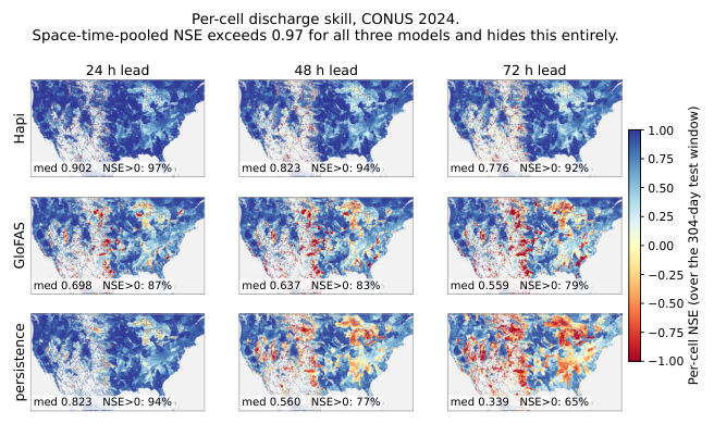
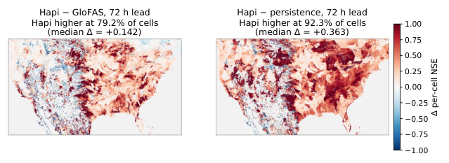
Appendix N Paired Block Bootstrap and Multiplicity Correction
The flood-detection numbers in Table 2 come from one 2024 test window whose daily values are strongly autocorrelated, so any statement about which model ranks higher needs an uncertainty estimate attached to it. We use a moving-block bootstrap [Künsch, 1989] over the time axis.
Resampling scheme.
Within each of replicates we draw blocks of consecutive days with replacement, truncate to days, and recompute the pooled contingency table. As specified in Section 4.1, RiverMamba’s latest discharge input is one day older than Hapi’s at the same nominal lead. The same block draw is applied to every model within a replicate, making the difference between two models the resampled quantity. The scheme preserves two statistical properties. Whole days are resampled, preserving within-day spatial dependence without treating the spatially clustered cells as independent observations. Within each replicate, F1 and SEDI are recomputed from the pooled resampled contingency counts.
Paired differences and marginal intervals.
Every model is scored on the same days, and their errors are strongly positively correlated because all models encounter the same sequence of hydrological conditions. Pairing accounts for shared day-to-day variation and reduces the variance of the difference relative to treating the model estimates as independent. Requiring the two marginal 95% intervals to be disjoint is more conservative than testing the paired difference directly. For the persistence and GloFAS comparisons, the marginal intervals overlap in every 72-h cell, whereas the paired test separates 20 of 28 cells. The paired test is therefore the appropriate inference for these correlated forecasts.
Block length.
The block must be long enough to preserve temporal dependence in the resampled series, which here is the daily count of cells exceeding the threshold. That dependence is not a single number: it falls steeply with return period, because frequent exceedances track slow catchment wetness while rare ones track individual storms. The observed series’ lag-1 autocorrelation and integrated autocorrelation time , truncated at the first non-positive , appear in Table 19.
| Return period (yr) | 1.5 | 2 | 5 | 10 | 20 | 50 | 100 |
|---|---|---|---|---|---|---|---|
| Exceeding cells per day | 7,883 | 3,453 | 689 | 270 | 126 | 59 | 36 |
| Lag-1 autocorrelation | 0.938 | 0.908 | 0.847 | 0.747 | 0.652 | 0.614 | 0.594 |
| (d) | 42.3 | 25.7 | 10.0 | 4.8 | 3.5 | 3.0 | 2.7 |
No single block length matches all seven columns. We set days near the upper end of the estimated dependence range and assess sensitivity to this choice below. At this block length, the 50- and 100-yr F1 and SEDI differences at 72-h lead against persistence and GloFAS are not significant after Holm correction. Their nonsignificance does not establish equivalence.
Sensitivity to the block length.
Re-running the whole procedure at block lengths from 7 to 60 days leaves the conclusion in place, as shown in Table 20. The surviving count moves over a narrow range with no trend across 7–45 days. At a block length of 60 days, each replicate draws five blocks and six blocks respectively, with the final block truncated as needed.
| Block length | 7 d | 15 d | 21 d | 30 d | 45 d | 60 d |
|---|---|---|---|---|---|---|
| F1, Hapi – persistence | 14 | 14 | 14 | 14 | 12 | 13 |
| F1, Hapi – GloFAS | 17 | 17 | 17 | 18 | 17 | 21 |
| F1, Hapi – RiverMamba | 21 | 21 | 21 | 21 | 21 | 21 |
| SEDI, Hapi – persistence | 12 | 12 | 12 | 12 | 12 | 12 |
| SEDI, Hapi – GloFAS | 17 | 16 | 16 | 17 | 16 | 19 |
| SEDI, Hapi – RiverMamba | 7 | 7 | 6 | 6 | 6 | 6 |
| Total (of 126) | 88 | 87 | 86 | 88 | 84 | 92 |
-values and multiplicity.
Each cell’s -value is the two-sided percentile bootstrap : the proportion of replicates whose difference falls on the opposite side of zero from the point estimate, doubled, with the correction of Davison and Hinkley [1997] so that no cell can report . The smallest attainable raw value is therefore . Because 21 (lead return-period) cells are inspected at once, we apply a Holm step-down correction [Holm, 1979] across each 21-cell family, separately per comparison and per metric, for six families and 126 cells in total. We define six families by crossing the two prespecified metrics (F1 and SEDI) with the three model comparisons (Hapi–persistence, Hapi–GloFAS, and Hapi–RiverMamba). Within each family, Holm correction covers all leads and return periods. Holm holds under arbitrary dependence between the tests, which is what this application needs: the seven return periods within a lead are nested, since every 100-yr exceedance is also a 1.5-yr exceedance. After correction the smallest attainable adjusted value is . At , this bound is , placing a comparison with no sign reversals just below because of Monte Carlo resolution. Increasing to reduces the bound to . Increasing from 1,000 to 10,000 changed few uncorrected decisions but lowered the minimum attainable adjusted -value.
Result.
The underlying bootstrap output also reports the paired point difference and its 2.5th–97.5th percentile interval for every cell. The intervals quantify effect-size uncertainty, whereas Figure 11 emphasizes the point differences and multiplicity-adjusted decisions. At 24-h lead Hapi’s F1 advantage over the GloFAS forecast is significant after correction at every return period from 1.5 to 100 yr. Hapi’s F1 advantage over RiverMamba survives correction in all 21 cells. The corresponding SEDI difference survives in six cells, at the 1.5- and 2-yr thresholds at each lead. Across all 126 cells, 88 survive correction, distributed 29 / 30 / 29 over the 24-, 48- and 72-h leads. None of the 126 comparisons shows a significant loss for Hapi after Holm correction. The seven negative point differences comprise six SEDI comparisons and one F1 comparison.

Appendix O Base-Rate-Invariant Skill and the Precision–Recall Decomposition
F1 depends on the event base rate, which falls by orders of magnitude as the return-period threshold rises. Consequently, F1 supports comparisons among models at a fixed threshold but not comparisons of skill across thresholds. For cross-threshold comparisons, we use SEDI because it remains non-degenerate as the event base rate tends to zero.
Figure 12 reports SEDI at the same 21 lead–threshold combinations as F1. Hapi’s 72-h SEDI decreases from 0.931 at the 1.5-yr threshold to 0.724 at the 100-yr threshold, indicating lower skill for rarer events under this base-rate-invariant measure. Among Hapi, GloFAS, and persistence, Hapi has the highest SEDI in 18 of the 21 comparisons, including all seven at both 48- and 72-h lead. The three exceptions are all at 24-h lead, at the 20-, 50- and 100-yr thresholds, where persistence leads.
The same contingency tables yield the precision, recall, and critical-success index (CSI) values in Table 21, with their geometric relationship shown in Figure 13. Figure 13 favors Hapi most clearly at 48- and 72-h lead, where it lies above and to the right of both baselines at every threshold and therefore occupies higher CSI contours. At 24 h, Hapi retains higher precision, but persistence has higher recall at the rarest thresholds, producing a trade-off rather than uniform dominance. Hapi’s advantage over the GloFAS forecast at 72-h lead is larger in precision than in recall at every return period: at the 5-yr threshold it gains in precision and in recall, and at the 100-yr threshold and , respectively. Hapi has higher recall than GloFAS at every lead–threshold combination.
At 72-h lead and the 1.5-yr threshold, its precision exceeds GloFAS by , its recall by , and its CSI by . Hapi also has higher CSI at 48 h ( versus ). GloFAS does not exceed Hapi on CSI in any comparison in Table 21. Persistence does so in one cell only, at 24-h lead and the 100-yr threshold, and by ( against ), consistent with its known short-lead advantage. Hapi’s precision exceeds its recall in every cell but one, corresponding to fewer predicted than observed exceedances. The exception is 72-h lead at the 100-yr threshold, where recall edges ahead by ( against ). Persistence’s precision and recall differ by at most over the test window.

| Return period (years) | ||||||||
| Model | Lead | 1.5 | 2 | 5 | 10 | 20 | 50 | 100 |
| Precision | ||||||||
| persistence | 24 h | 0.836 | 0.800 | 0.709 | 0.627 | 0.562 | 0.496 | 0.470 |
| persistence | 48 h | 0.726 | 0.672 | 0.544 | 0.434 | 0.353 | 0.275 | 0.233 |
| persistence | 72 h | 0.653 | 0.590 | 0.447 | 0.334 | 0.256 | 0.177 | 0.140 |
| GloFAS | 24 h | 0.778 | 0.723 | 0.590 | 0.478 | 0.405 | 0.314 | 0.267 |
| GloFAS | 48 h | 0.754 | 0.688 | 0.538 | 0.417 | 0.336 | 0.243 | 0.190 |
| GloFAS | 72 h | 0.727 | 0.656 | 0.493 | 0.362 | 0.274 | 0.179 | 0.127 |
| Hapi | 24 h | 0.912 | 0.905 | 0.857 | 0.787 | 0.713 | 0.641 | 0.574 |
| Hapi | 48 h | 0.859 | 0.837 | 0.737 | 0.609 | 0.486 | 0.352 | 0.272 |
| Hapi | 72 h | 0.827 | 0.799 | 0.684 | 0.538 | 0.413 | 0.274 | 0.208 |
| Recall | ||||||||
| persistence | 24 h | 0.836 | 0.799 | 0.708 | 0.627 | 0.562 | 0.496 | 0.470 |
| persistence | 48 h | 0.726 | 0.671 | 0.544 | 0.434 | 0.353 | 0.275 | 0.233 |
| persistence | 72 h | 0.653 | 0.590 | 0.447 | 0.334 | 0.256 | 0.177 | 0.140 |
| GloFAS | 24 h | 0.767 | 0.713 | 0.577 | 0.467 | 0.388 | 0.299 | 0.261 |
| GloFAS | 48 h | 0.741 | 0.682 | 0.533 | 0.410 | 0.330 | 0.234 | 0.191 |
| GloFAS | 72 h | 0.714 | 0.650 | 0.492 | 0.367 | 0.280 | 0.188 | 0.142 |
| Hapi | 24 h | 0.859 | 0.824 | 0.727 | 0.631 | 0.535 | 0.442 | 0.395 |
| Hapi | 48 h | 0.808 | 0.764 | 0.651 | 0.535 | 0.436 | 0.323 | 0.266 |
| Hapi | 72 h | 0.775 | 0.726 | 0.598 | 0.470 | 0.371 | 0.253 | 0.209 |
| CSI | ||||||||
| persistence | 24 h | 0.719 | 0.666 | 0.549 | 0.457 | 0.391 | 0.329 | 0.307 |
| persistence | 48 h | 0.570 | 0.505 | 0.373 | 0.277 | 0.214 | 0.160 | 0.132 |
| persistence | 72 h | 0.485 | 0.418 | 0.288 | 0.201 | 0.147 | 0.097 | 0.075 |
| GloFAS | 24 h | 0.629 | 0.560 | 0.412 | 0.310 | 0.247 | 0.181 | 0.152 |
| GloFAS | 48 h | 0.597 | 0.521 | 0.365 | 0.260 | 0.199 | 0.136 | 0.105 |
| GloFAS | 72 h | 0.563 | 0.485 | 0.327 | 0.223 | 0.161 | 0.101 | 0.072 |
| Hapi | 24 h | 0.794 | 0.759 | 0.648 | 0.539 | 0.441 | 0.355 | 0.306 |
| Hapi | 48 h | 0.713 | 0.665 | 0.528 | 0.398 | 0.298 | 0.202 | 0.155 |
| Hapi | 72 h | 0.667 | 0.613 | 0.468 | 0.335 | 0.243 | 0.151 | 0.116 |