Design and pricing of a transparent parametric-modeled loss CAT bond: application to German windstorm
Abstract
Catastrophe (cat) bonds overcome some lack of reinsurance by sourcing capacity from the wider capital markets. We present a new type of cat bond addressing the known trade-off between moral hazard and basis risk. As our main contributions we propose a trigger mechanism which is entirely transparent and simpler to evaluate compared to indemnity modeling techniques, as well as a methodology to price this cat bond. This is relevant for insurers and public authorities in a world where natural disasters are occurring with increasing frequency and severity due to climate change, but also for players willing to enter the cat bond market for whom the lack of transparency of this asset class has been a significant obstacle. Our trigger is derived from a cost random field which separates the physical hazard, a vulnerability function and the exposure. This allows the trigger to take a flexible form between parametric and modeled loss, in case exposure is taken into account. We present a case study based on historical windstorm events impacting Germany. Using wind speed data from historical storms, we fit a max-stable random field on a resolution which is standard in the reinsurance industry. The availability of industry loss and exposure data allows us to calibrate the vulnerability component to historical observations. Besides measuring the basis risk associated with our trigger, we perform a full model assessment and discuss numerical results.
1 Introduction
Catastrophe (cat) bonds transfer peak insurance risks in a securitized form to capital markets. The underlying risk most often being the occurrence of natural catastrophes, cat bonds are lightly correlated to other asset classes such as equities or traditional bonds, and generally offer attractive yields compared to other products with similar levels of risk; see, e.g., Cummins (2008). They are typically fully collateralized and hence do not include any (or very low) counterparty default risk as the proceeds are invested in government bonds with very low credit risk.
Cat bonds can be found in the market under various triggering schemes: parametric, modeled loss, industry loss index, indemnity or a combination thereof. An essential aspect to consider when designing the trigger is to strike an appropriate balance between basis risk and moral hazard, both from the perspective of the sponsor and the investors. Basis risk captures the possibility of a mismatch between the losses suffered by the sponsor and the actual payout from the bond. Moral hazard corresponds to the risk that the parties involved may influence the payment outcome. Decreasing the potential for moral hazard leads to higher transparency. Cat bond prices are obtained by running vendor models (Moody’s RMS, Verisk and CoreLogic being the main ones) which are like black boxes as their modeling assumptions are not public. This means that the risk modeling and ultimately the pricing is not performed in a transparent way and cannot be computed independently by the investor.
In this work, we propose a new blended trigger which is more complex than parametric products currently available in the market. Such triggers are typically based on physical characteristics of the event underlying the risk such as magnitude and depth for earthquakes, storm surge height for coastal windstorms, or minimal central pressure for hurricanes. Our approach allows for a more flexible modeling using a cost field which incorporates exposure and vulnerability, see Section 3, while retaining the high degree of transparency typical of parametric triggers. It additionally offers the possibility to account for industry exposure, making the trigger closer to modeled loss triggers in this case, albeit without resorting to complex physical cat models from modeling agencies. We illustrate the positioning of our proposal for a blended trigger relative to common trigger types in terms of transparency and basis risk in Figure 1. We discuss the various trigger types found in the cat bond market in Section 2.1, below.
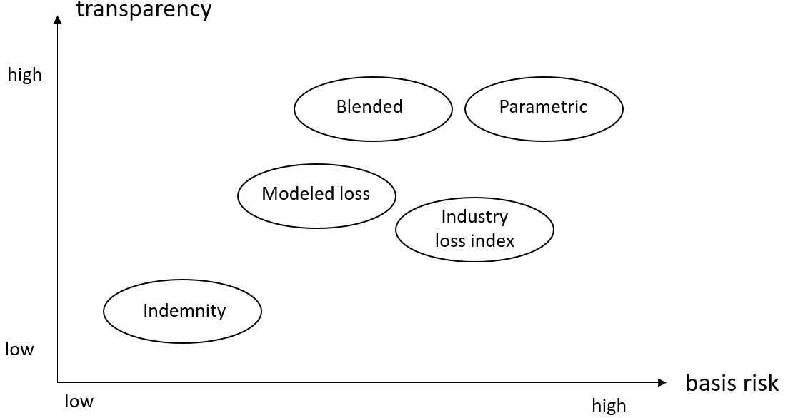
Our approach builds on hazard data compiled by trusted and reputed institutions such as governmental weather agencies and which are available to both the investors and the sponsor. The availability of industry loss data further allows us to calibrate the trigger to observed losses. We believe this methodology is beneficial for combinations of regions and perils where cat models are either unavailable or cannot be trusted, and where insurers do not have any historical loss data at their disposal; otherwise more standard techniques such as frequency-severity loss models or vendor cat models can be used. For regions and perils where cat models are available, our model provides an additional view of risk based on a series of assumptions that are disclosed to both parties to the transaction, which is not the case for vendor models that need to be licensed. Even though our trigger is also derived from a frequency-severity-type model, we stress that the severity component is based on the theory of spatial extremes and not on the more common Pareto distribution used in actuarial modeling.
Underlying our loss model, we define a cost field which takes into account the hazard, vulnerability and exposure, as is typically done in cat modeling. The cost field is itself derived from a max-stable random field, which is commonly used in the modeling of spatial extremes but has so far not been applied in the context of cat bonds. Furthermore, we propose a fully transparent pricing formula in a contingent claims setting, allowing both parties in the transaction to compute the price from the loss model.
We refer the reader to Cummins (2008) and Ben Ammar et al. (2015) for a general overview of the cat bond market. Parametric trigger design with a discussion of basis risk is explored in Goda (2013), Pucciano et al. (2017) and Goda et al. (2019) with applications to Turkey earthquake bonds, and in Franco (2010) and Calvet et al. (2017) for Costa Rica earthquake bonds. However, in each case, events are generated from complex cat models and not from models fitted to publicly available data. In more recent works, Tan and Zhang (2023) design weather index insurance products for US corn production using penalized splines, whereas Gao et al. (2023) consider a spatio-temporal framework in the context of crop insurance risk modeling. A method using univariate extreme value theory (EVT) is discussed in Zimbidis et al. (2007) and applied to the pricing of cat bonds on Greek earthquakes, however, spatial dependence between locations is not taken into account. In the context of hurricane frequency modeling, Chang et al. (2020) propose a regime-switching Poisson process based on climate indices. An option pricing approach is presented in Chang et al. (2022) for hurricane bonds with two severity formulations depending on physical characteristics of the hazard, however with no consideration of vulnerability and exposure. Extending the scope of covered risks under cat bond transactions, Xu and Zhang (2021) present a modeling and pricing approach for (non-stationary) data breach risks.
One of the first attempts to price cat bonds in a contingent claim framework goes back to Cox and Pedersen (2000), where an equilibrium pricing model is introduced. It assumes that financial and insurance technical (catastrophe) variables are independent. We will use this setting as the basis for pricing our product. The approach proposed in Lee and Yu (2002) relies on a contingent claim model to price default-risky cat bonds (which is less of an issue nowadays due to the SPV investing the proceeds in highly-rated securities) in the presence of moral hazard and basis risk, using a generic compound Poisson loss model with log-normal severities. These two methods consider cat bonds as zero-beta securities, i.e., no natural catastrophe risk premium is assumed, see also Nowak and Romaniuk (2013). Since CAT bond payouts cannot be replicated by securities available in financial markets, pricing has to performed under an incomplete market framework. Indifference pricing techniques via expected utility are discussed in Egami and Young (2008) and Zhu (2011). The valuation of so-called Wincat coupons from the Winterthur Insurance convertible bonds on an indemnity basis is investigated in Schmock (1999) with a discussion of model risk, whereas Shao et al. (2015) consider multiple financial and insurance variables with an application to cat bonds covering California earthquake risk.
An alternative way to price securities in an incomplete market is by using the Wang transform, see Wang (1996), Wang (2000), and Wang (2002). In the context of cat bond pricing, this approach has been investigated for mortality bonds in Lin and Cox (2005), Lin and Cox (2008) and Chen and Cox (2009), for longevity bonds in Denuit et al. (2007) and Chen and Cummins (2010), and for earthquake bonds in Tang and Yuan (2019). A comparison of various premium calculation methods is undertaken in Galeotti et al. (2013) and it is shown that the Wang transform performs best in terms of prediction accuracy. An arbitrage approach built on risk indices that obey jump-diffusion processes is presented in Vaugirard (2003). The issue of non-tradeability of catastrophe risk in the framework of no-arbitrage pricing theory is tackled in Gatzert et al. (2019) using index-linked products.
Another line of research focuses on econometric models for pricing cat bonds, see, e.g., Lane (2000), Bodoff and Gan (2009), Papachristou (2011) and Gürtler et al. (2016). Such models regress historical cat bond spreads on observable variables such as the expected loss, see Braun (2016) where the whole universe of bonds issued between 1997 and 2012 is considered. An approach based on random forests to predict spreads in the primary cat bond market has been introduced in Makariou et al. (2021) and builds on a comparative analysis between various machine learning methods in Götze et al. (2020). In our setup, we consider the spread as exogenously given and playing the role of an input variable to derive the cat bond price.
In the cat bond market, several transactions have been structured using a parametric trigger built on transformations of a variable characterizing the underlying risk, for example, wind speeds in the case of windstorm risk. However, these constructs are confidential and only very limited information is available in the public domain. The trigger we propose accounts for both vulnerability and exposure and as such, it aims at achieving lower basis risk while keeping the transparency inherent to parametric triggers. We are not aware of any academic publication that examines such a trigger within a detailed concrete application. Moreover, to the best of our knowledge, this is the first attempt to price cat bonds using max-stable models. This allows us to consider several locations and the spatial dependency between them, as opposed to univariate methods such as Zimbidis et al. (2007). One can them embed the loss model into a pricing framework inspired by the approach developed in Cox and Pedersen (2000), by assuming independence between financial and insurance technical variables. We price our cat bond under a risk-neutral measure implied by the Wang transform, see Galeotti et al. (2013) and Tang and Yuan (2019). Using this framework, investors are able to challenge each modeling assumption and to independently compute the bond price. Moreover, in case of an event, the trigger can be evaluated using publicly available data. We investigate basis risk under several trigger specifications and perform a full model assessment by validating the hazard model using wind speed data, the vulnerability model using industry insured loss data per event as well as exposure data. Moreover, we specify a frequency distribution describing the number of events per year.
The remainder of the paper is structured as follows. In Section 2, we provide a general description of the cat bond asset class, present a pricing formula, and lay out the necessary mathematical building blocks for our framework. Section 3 is dedicated to our main contributions: the novel trigger and the pricing methodology based on our loss model. Finally, we present a real case study based on German windstorm events to support our findings, accompanied with numerical results in Section 4.
2 Cat bonds and max-stable random fields
In this section, we first provide a general overview of cat bonds and discuss how the pricing is performed, both in the literature and in practice. This opens the door to our main contributions presented in Section 3. Then, we briefly review max-stable random fields, as we will use such fields to model the weather variable underlying the cat bond in our case study in Section 4.
2.1 Overview of cat bonds
Cat bonds play a major role in the alternative risk transfer (ART) market and, in particular, within the insurance-linked securities (ILS) asset class, see Cummins (2008). Investors’ appetite has concentrated in this segment of the market as a higher level of transparency as well as liquidity is present in the cat bond market compared to more private and bespoke ILS structures. As such, they complement the reinsurance market by providing additional risk-bearing capacity. We refer to Ben Ammar et al. (2015) for a more complete introduction to the ART market and other standard financing tools such as industry loss warranties (ILW), reinsurance sidecars or collateralized reinsurance.
We illustrate the structure of a cat bond in Figure 2. The so-called special purpose vehicle (SPV) issues the cat bond notes to investors and invests the funds received in highly-rated securities, e.g., U.S. money market funds, making the risk transfer fully collateralized and highly reducing the counterparty default risk. In exchange for bearing the catastrophe risk, investors receive on top of the (floating) risk-free rate a fixed premium or risk spread from the sponsor, which is usually an insurer, a reinsurer or a state agency such as the California Earthquake Authority (CEA). Investors in cat bonds typically range among dedicated ILS funds, hedge funds, pension funds, and (re)insurers.
A cat bond pays off contingent upon a suitably predefined catastrophe event occurring during the risk period, such as a North American hurricane, a European windstorm or a Japanese earthquake. The bond is triggered in case some (proxy) quantity related to the loss and depending on the type of trigger, see the discussion below, exceeds some threshold called the attachment point. In some instances a second (higher) threshold is specified, called the exhaustion point, which is the level at which investors would face a full investment loss. The payout structure can then take several forms, e.g., step-wise, linear or binary. In case a triggering event occurs during the lifetime of the contract, the proceeds from the collateral account are used to cover the sponsor’s losses. In the event of a full loss the principal is not returned to the investors, see Figure 3. In case of a partial loss, i.e., a loss between the attachment and the exhaustion point, only the impacted part of the principal is disbursed to the sponsor. If there are no losses over the lifetime of the contract that are above the attachment point, investors receive the entire principal alongside the earned investment return, see Figure 4.
Cat bonds have a proven track record of delivering higher returns11 1 This can however be questionable since in some instances, the risk is not fully understood and what is observed as excess return may just be a margin to compensate for uncertainty. This has been the case for some recent wildfire transactions. than other asset classes with a similar level of risk and of bringing diversification to portfolios due to their low correlation with other instruments, see, e.g., SwissRe (2011). Given their multi-year duration, generally up to 3-4 years, insurers and reinsurers holding these bonds can achieve a partial decoupling from the pricing cycle in the traditional reinsurance market, reducing earnings volatility. In addition, booking technical provisions for ILS allows a sponsor to reduce its minimum capital requirement. Moreover, unlike reinsurance contracts, cat bonds are tradeable over-the-counter in secondary markets. Finally, they allow accessing the much larger capital markets and provide much needed capacity during hard stages of the reinsurance cycle, i.e., when reinsurance is more expensive than average. On the downside, the costs associated with structuring and modeling can be quite high but they should always be put into perspective with brokerage fees and commissions in reinsurance. In addition, in terms of capacity, investor capital is not permanent as other asset classes with higher yields might be more attractive.
In the case of a cat bond, there is usually a modeling agency (most often among RMS, Verisk or CoreLogic) providing an independent modeling assessment of the underlying risk and reward structure of the bond: it computes the attachment probability (probability that the loss reaches the attachment point), the exhaustion probability (probability of a full loss) and the expected loss. On top of the floating rate generated from the risk-free collateral account, a risk spread is paid to investors. The so-called multiple is the ratio of this risk spread over the modeled expected loss.
A cat bond can be structured to provide per-occurrence cover, meaning per-event exposure, or aggregate cover, that is, exposure to multiple events over the course of each annual risk period. Let us note that other types of risks can be covered through ILS structures, for instance, mortality, longevity, mortgage or casualty risks. In the sequel we focus on natural catastrophe risks and specifically on aggregate covers.
Cat bonds come with various triggering schemes, determining whether the entire or part of the principal is used to cover losses to the sponsor following an event (Ben Ammar et al., 2015, see, e.g.,):
- •
Industry loss index: payout based on the total loss to the insurance industry, for example, using Property Claims Services (PCS) or PERILS data.
- •
Pure parametric index: payout depends on hazard characteristics such as earthquake magnitude, storm central pressure or wind speed.
- •
Modeled loss: recovery depends on loss modeled by agencies (RMS, Verisk, CoreLogic) using the event characteristics, exposure data and the vulnerability module of the cat model.
- •
Indemnity: recovery is entirely based on the loss experienced by the sponsor.
Parametric index triggers constitute a refinement of pure parametric triggers. They allow the trigger to be more flexible by introducing additional variables such as the radius of the storm or the geographical coordinates of the insured risk, (SwissRe, 2011, see). They are equally transparent and additionally reduce basis risk, that is, the risk of a mismatch between the cat bond payout and the losses to the sponsor. Indemnity remains the most common trigger type in the market, followed by industry loss index (Carelus, 2018, see). On the other hand, moral hazard could arise from the lack of transparency of the bond. Indeed, with an indemnity trigger, although there are contractual limitation factors to control exposure growth and yearly resets to adjust the attachment point and the expected loss (Ben Ammar et al., 2015, see), an insurer may submit an inaccurate loss report or could decide to underwrite more contracts in regions covered by the bond. Sponsors and investors thus face a trade-off between transparency and basis risk. Investors will generally favor the transparency and reduction in moral hazard offered by parametric covers. The latter additionally provide a faster settlement due to contract terms and the simplicity to determine whether the threshold has been met or not. The sponsor may also have an incentive for risk transfer products to pay out very fast. This is the case for World Bank transactions where funds need to be disbursed as quick as possible to rebuild in countries that get hit by a natural disaster. On the other side of the spectrum, sponsors will tend to prefer indemnity triggers as these minimize basis risk. Finally, modeled loss triggers partially offset the moral hazard associated with indemnity triggers, while displaying a level of basis risk which is lower than for parametric triggers. However, the industry models, albeit constantly progressing in terms of data capture, accuracy and coverage, might still exhibit some model risk. Moreover, they are based on stochastic event catalogs which are difficult to challenge due to intellectual property and their lack of transparency.
A new type of product, known as hybrid cat bonds, is proposed in Barrieu and Loubergé (2009) to protect investors from a stock market crash on top of the exposure to catastrophe risk. Hybrid cat bonds can also be understood as bonds where the trigger is a mixture between different types of triggers, such as parametric and industry loss index. Various clustering algorithms are tested in terms of their classification accuracy for a binary trigger in Calvet et al. (2017), with a case study based on a catalog of stochastic earthquake events in Costa Rica. The results are benchmarked with the optimal trigger obtained from a genetic algorithm presented in Franco (2010). In both cases, the trigger is parametric; however, it is elaborated on synthetic data and not on observations. This could raise the issue of complexity with regards to investors. A distinction in the literature is set between so-called first generation or "cat-in-a-box" triggers (Franco, 2010, see) and second-generation triggers (Goda, 2013, see), where in addition the reduction in basis risk is highlighted when using step-wise payouts instead of binary payouts. First-generation triggers consider the physical characteristics of the covered event (e.g., for an earthquake, the depth, magnitude and coordinates of the epicenter). The attachment can be made dependent on the event magnitude and the location by defining a polygonal grid over the covered region. In this way, varying magnitudes within each polygon need to be attained to trigger a payout. In turn, second generation triggers are built from spatially distributed features, e.g., stations reporting wind speed or spectral acceleration, with weights that can be selected at each station in order to reflect the sponsor’s exposure in the region, see, for example, the Bosphorus 2015 transaction covering earthquakes in Turkey22 2 https://www.artemis.bm/deal-directory/bosphorus-ltd-series-2015-1/. Building on this work, Pucciano et al. (2017) and Goda et al. (2019) study the interplay between the required complexity of the trigger formulation and the distribution of the reporting stations in terms of their vicinity with respect to insured assets.
Arguably, the most complex parametric trigger was the Compass Re II bond issued on behalf of AIG in 2015 for covering hurricanes in the US33 3 https://www.artemis.bm/deal-directory/compass-re-ii-ltd-series-2015-1/. The trigger was a functional of the latitude and longitude at landfall, the radius of the storm and the maximum sustained wind speed. The inclusion of the landfall coordinates allowed the sponsor to calibrate the trigger to be more responsive to areas with peak exposure. We could not find any successor transaction of this Compass Re deal. Among European windstorm transactions, Pylon II Capital was an innovative cover for protecting French utility Électricité de France44 4 https://www.artemis.bm/deal-directory/pylon-ii-capital-ltd/. Blue Fin Re was another parametric bond covering European windstorm and was issued in 2007 on behalf of Allianz55 5 https://www.artemis.bm/deal-directory/blue-fin-ltd/. There is, however, no publicly available information on the exact formulation of the trigger.
Parametric triggers for outstanding cat bonds have been used for certain World Bank sponsored transactions (first generation trigger for Mexico earthquake and hurricane, and for Jamaica hurricane), and public authorities such as the Metropolitan Transportation Agency in New York, with the 2020 MetroCat bond covering storm surge and earthquake using a second-generation trigger with a binary payout66 6 https://www.artemis.bm/deal-directory/metrocat-re-ltd-series-2020-1/.
This shows that some interesting triggering mechanisms have been elaborated in the industry but remain confidential, and in the case where information is available in the public domain, for example, on the website https://www.artemis.bm, the trigger structure is not presented in detail. We attempt to address this gap with a parametric trigger for which we lay out all modeling assumptions and which can be compared in terms of basis risk to trigger formulations which have been used in practice.
2.2 Spread and bond price
As opposed to econometric models which regress historical bond spreads on observable variables such as the expected loss, covered territory, sponsor, spreads on corporate bonds with comparable ratings, and latent variables such as the stage of the reinsurance cycle (Braun, 2016, see) in the present approach we consider the spread as exogenously given and playing the role of an input variable in the formulation of the bond price. Under this scenario, cat bonds are priced in an incomplete market framework. Since the underlying process (natural catastrophe occurrence) triggering the event is not a tradeable security, it is not possible to construct a replicating portfolio of assets to match the payoff of the bond.
Suppose a sponsor wishes to issue a cat bond with maturity years. We discretize the time interval in yearly units, and we say that a catastrophe occurs in year if it takes place in the time interval for We denote the attachment point of the bond as and the exhaustion point by these two quantities being contractually determined before inception. The investors receive in exchange for the risk they bear a coupon, which consists of a fixed spread given in percentage per annum of the face value , on top of a floating short rate (which is usually the 3-month US money market funds rate).
Assume all random variables defined in the sequel live in the filtered probability space for a filtration As in Cox and Pedersen (2000), under our risk-neutral pricing measure , we assume that financial market (short rate) variables and insurance technical (catastrophe) variables are independent, which leads to a decoupling of under into
where for all it is assumed that is the smallest -field containing all events of and see Wüthrich (2016). We assume that the filtrations and are independent under
We consider at this stage a general model for the loss process with finite time horizon , where is the loss in year , for We assume that the components are independent and identically distributed under and that the loss process is -adapted. This general model could be either a cat model or a standard frequency-severity model. In Section 3, we will present a loss model that is tailored to our problem. For the purpose of expressing the stream of cash flows, we define the stopping time as
where we follow the convention if for all
Losses below the attachment point are fully assumed by the sponsor, whereas a loss above the exhaustion point leads to a full loss of the principal for investors. Losses between the attachment and the exhaustion points trigger the bond and entail only a partial repayment of principal to investors. In case a triggering event occurs before maturity, investors receive the amount , where corresponds to the proportion of the face value which is lost at time Typically, a piecewise linear form in the loss is specified, that is, for
In the limiting case where we obtain a binary loss, that is, a full loss to the investors when the bond is triggered and a full recovery of principal otherwise. Hence, this formulation also covers cat bond deals without exhaustion points. Let us note that other formulations for the payoff can be equally considered, such as a stepwise constant structure which is often found in parametric covers, where the level depends on some physical characteristic of the peril, e.g., the earthquake magnitude, as in Zimbidis et al. (2007). Assume that coupons are paid at the end of each year, contingent on no loss above the attachment point. The total cashflow is obtained by taking the sum of the principal redemption and the coupons. The former can be written at time as
where for all is -measurable since the loss process is -adapted. In other words, we assume that the residual principal is paid at the end of the year in which the loss occurred. We will assume Vasicek dynamics for the short rate, although any other stochastic model that is analytically tractable can be used without having to rely on simulation. The short rate process denoted by is thus governed by
with initial value where and denote the speed of mean reversion, the level of mean reversion and the volatility, respectively, and where is a Brownian motion under that is -adapted. To derive the distribution of the loss variable under we introduce the Wang transform, see Wang (1996); Wang (2000); Wang (2002); Wang (2004)
| (1) |
where is a distortion function which is non-decreasing and right-continuous, with and such that for is a skewness parameter and is the standard normal distribution function. The parameter can be calibrated so as to ensure the bond is valued at par, see Tang and Yuan (2019), and can be interpreted as the catastrophe risk premium as it reflects the extent to which the distribution of the catastrophe risk variable needs to be skewed towards the right for risk-neutral pricing purposes. Assume that the loss random variables are also i.i.d. under with We define the (distorted) distribution of under as
The coupon at time is given by and this quantity is -measurable for all This leads to the following expression for the price of the cat bond at :
| (2) |
where denotes the value of the bank account at time Since is an affine process, one can write, see, e.g., Brigo and Mercurio (2006),
| (3) |
where the exact forms of the functions and are given in Brigo and Mercurio (2006). In order to simplify the computation of the cat bond price, we consider the -forward probability measure which is equivalent to and is defined by the Radon-Nikodym derivative
| (4) |
We note that under this measure change, the independence between insurance technical and financial variables is preserved. The dynamics of the short rate process under for are then given by
where is a -Brownian motion that is -adapted and satisfies
for see Brigo and Mercurio (2006). Solving this stochastic differential equation, we obtain the mean of the Vasicek process at time under :
| (5) |
The independence between financial and insurance technical variables allows to decouple the expression in (2) as follows
| (6) |
We can then compute using the -forward measure defined in (4), and (5). We derive the expectations and using (3).
Under the assumption of independent components of the loss process, the stopping time decouples similar to a geometric distribution, i.e.,
Under the latter assumption, we obtain analogously
One can consider the case without loss of generality as In this case, the expression above reads
In Section 4.6, we will evaluate the price at (6) from a sample of realizations of based on empirical estimates of the attachment probability and the exhaustion probability The empirical distribution of under is obtained by applying the Wang transform in (1) to the empirical distribution of under . The empirical counterpart of the probability is given by
By definition of
We consider the reordered sample so that
The empirical counterpart of the expectation is then obtained using the Wang-transformed probability weights
where Note that the probability of attachment and the probability of exhaustion are higher under due to the distortion introduced by the Wang transform. In Figure 5 (left panel), we show how the empirical cumulative distribution of gets distorted when switching from to The right panel in Figure 5 is based on a smaller sample of simulations to visualize how the Wang transform distorts the probability weights under to under .
2.3 Max-stable random fields
Throughout, denotes the supremum. Moreover, and stand for equality and convergence in distribution, respectively. In the case of random fields, distribution has to be understood as the set of all finite-dimensional distributions.
A random field on is said to be max-stable if there exist continuous functions and on such that if are independent replications of , then
for all Moreover, it is called simple if it has standard Fréchet margins, i.e., for all , .
Max-stable random fields are ideally suited to the modeling of pointwise maxima. Let be independent replications of a random field on (for instance, the field of wind speed values in the case ) and let and be sequences of functions. If there exists a non-degenerate random field on such that
then is necessarily max-stable (de Haan, 1984, e.g.,). More generally, as noted in, e.g., Huser and Davison (2014, Section 2.3), max-stable fields provide appropriate models for extremes of individual observations.
We now provide a probabilistic construction of simple max-stable fields that can be leveraged to build parametric max-stable models. Let be the points of a Poisson point process on with intensity function and let , be independent replications of a random field which are independent of the and such that, for all , . Then the field defined on by
| (7) |
is simple max-stable, see de Haan (1984).
This so-called spectral representation has been exploited to define the Brown–Resnick, extremal-, Schlather, and Smith max-stable models that we will use in Section 4. Recall that a random field has stationary77 7 Throughout the paper, stationarity refers to strict stationarity. increments if the distribution of the field , , does not depend on the choice of . If the increments of have a finite second moment, the semivariogram of is
where stands for the variance. Let , be a centered Gaussian random field with stationary increments and with semivariogram . Then the field defined by (7) with
is referred to as the Brown–Resnick random field associated with the semivariogram (Brown and Resnick, 1977; Kabluchko et al., 2009). It is stationary with a distribution fully described by (Kabluchko et al., 2009, Theorem 2 and Proposition 11, respectively). A commonly used semivariogram is
| (8) |
where denotes the Euclidean norm, and and are the range and smoothness parameters, respectively.
Let , , be a stationary standard Gaussian random field, let denote the gamma function. Then taking in (7)
where is the number of degrees of freedom, yields the extremal- model and one can verify that for all (Opitz, 2013). The fact that any correlation function can be used for offers flexibility. In the following, we will consider the Whittle-Matérn, powered exponential and Cauchy functions.
The Cauchy function is
| (9) |
where is the Euclidean distance between two locations, and are the range and smoothness parameters, respectively, and it is common practice to add a nugget parameter to the correlation function as follows
The case leads to the so-called Schlather model (Schlather, 2002). Under some conditions, the extremal- random field converges to the Brown–Resnick field as .
The Whittle–Matérn correlation function is
for range and smoothness parameters and respectively, and where is the modified Bessel function of the third kind with order
The powered exponential correlation function is
for and
The Smith random field with covariance matrix (Smith, 1990) corresponds to the Brown–Resnick field associated with the variogram , , where ′ designates transposition; see, e.g., Huser and Davison (2013).
A well-known measure of spatial dependence for max-stable fields, which is also frequently used for goodness-of-fit assessments, is the bivariate extremal coefficient function (Schlather and Tawn, 2003, e.g.,). It satisfies, for all ,
where is simple max-stable.
In practice, max-stable fields are not necessarily simple but have generalized extreme-value (GEV) univariate marginal distributions. If is a max-stable field with location, scale and shape functions , and , we can write
| (10) |
where is simple max-stable, see Koch and Robert (2022).
3 Main contributions
In Section 2.1, we have outlined the types of parametric triggers which have been used for previous cat bond issuances, as well as proposals from the academic literature. In this section, we present our main contributions: a new trigger type which can take a flexible form between parametric and modeled loss, and an approach to compute the price of the cat bond.
Consider a cat bond covering the insured claims for a specific type of natural disaster (e.g., extra-tropical or tropical cyclones) on a given region of interest and during a one-year period. The covered area can be an entire country, several countries or a particular subregion within a country where the sponsor is seeking coverage.
We consider a discretized region in the style of second generation parametric triggers, that is, we assume that we have sites that are representative of in terms of insured claims. Each site is characterized by its longitude, latitude and altitude, that is, for In the ideal scenario, each site would correspond to a policy as this would allow to consider the exposure at each insured location and enable a closer calibration of the trigger to actual losses. However, this is not realistic in practice as exposure data is usually available only on an aggregated level, for example, administrative regions. Therefore, sites must be chosen to reflect the exposure in each region. We will discuss various modeling options in Section 4.1.
Let denote the number of events of the considered type occurring during the one-year period under study. We propose to model the spatial field of insured claims triggered by the -th event, for , using a field that is constructed solely from transformations of publicly available hazard-related physical fields (e.g., maximal wind speed) and, possibly, freely accessible industry exposures. Otherwise, predefined exposures in the neighborhood of each can be used. The mentioned transformations are damage functions that map the physical features of the hazard to destruction percentages.
Mimicking the structure of cat models, we approximate the actual cost associated with event by the cost field
| (11) |
where is a damage function, corresponds to a functional of the environmental variable characterizing the physical hazard for event (for example, the field of maximum wind speeds), and represents the (deterministic) exposure field; see Koch (2017).
We assume that the fields , for , are independent and identically distributed (i.i.d.), and that the damage function is identical across events. Under these assumptions, the resulting cost fields are also i.i.d. The assumption on is made for simplicity. However, in practice, one would expect that for two successive events occurring close in time and with similar wind speeds, the insured loss from the second event would be lower due to damage already caused by the first. In the absence of loss data, the damage function is typically chosen based on physical and engineering principles and expert opinion. Otherwise, it can be calibrated empirically; see Section 4.2. If exposure data are not available, a constant exposure field may be specified for simplicity. Otherwise, several approaches can be used to model the exposure component of the cost field. It can take, for instance, a parametric form where is a function of latitude and longitude only. Alternatively, it may depend on a set of socio-economic variables
where and are the number of inhabitants, the mean wealth per inhabitant, the penetration rate of insurance and the orographic exposure at site respectively. The latter variable captures the protection effect for a specific site: for example, if buildings at are surrounded by very high buildings, there is a high protection effect. On the other hand, if is on top of a hill, it will be much more exposed to wind (but also much less exposed to, e.g., flood). This alternative specification for the exposure component could be the subject of further research.
Note that, for each event, we assume the same damage function. In Section 4.2, we will consider yearly exposure fields which take into account the evolution of sums insured. The iid assumption for event costs is made for simplicity. The cost field in (11) considers one environmental variable. However, one could extend our approach to account for a multidimensional set of environmental variables.
We define our annual loss trigger as
| (12) |
where is the loss from event We will refer to realizations of and as annual loss trigger realizations and event loss trigger realizations, respectively. We assume that are i.i.d. and are independent of . By construction, realizations of can be computed using only publicly available data from reputed and unbiased third parties (weather or geological agencies and insurance industry loss aggregators). Unlike the case of indemnity triggers, it does not require the knowledge of real losses to the insured, and unlike modeled loss triggers, no access to vendor cat models is needed. This results in full transparency of the triggering mechanism and no moral hazard, as in the case of parametric bonds. At the same time, the proposed trigger can be a better proxy for the real loss than triggers commonly used for parametric bonds which generally do not account for damage functions and exposure. Indeed, such triggers, being based on characteristics of the hazard such as moment magnitude for earthquakes or minimum central pressure for cyclones, may not correlate sufficiently enough with actual losses. Our trigger incorporates transformations that allow us to take exposure via the field and vulnerability via the damage function into account. As a result, we expect basis risk to be reduced. In its spirit, the trigger we propose goes in the direction of a modeled loss trigger since vulnerability curves and potentially exposures can be used, without being one since no cat models are involved. Hence, our trigger potentially offers a good balance between moral hazard and basis risk by keeping the transparency of a parametric trigger while simultaneously reducing its basis risk. The latter stems from two sources: the choice of the sites and the specification of the cost field Note that there is no basis risk from the number of events as one would consider the observed number of events during the period under consideration. Moreover, the trigger could be useful for new regions where there are no cat models at hand, in particular, for emerging markets. In such cases, there are typically no loss data available (and when it is, the calculation of claims can be opaque and payouts can take several months) and often only simple parametric solutions such as first generations triggers, see Section 2.1, are offered.
For indemnity-based bonds, moral hazard might appear as the sponsor may have incentives to compute the trigger in its favor by inadequately reporting the incurred loss. In case the information is not transferred in an open way, investors may not be able to challenge the trigger evaluation even if it is done properly by the sponsor. Indeed, there are historical precedents of indemnity triggers which have gone to court, due to ambiguities in the loss classification and inadequate loss reporting, as in the case of cat bond Mariah Re which defaulted following the active U.S. tornado season in 201188 8 https://www.artemis.bm/deal-directory/mariah-re-ltd-series-2010-1/.
Our pricing methodology also offers advantages in terms of transparency. We need a good statistical model for the field in (11) in order to mitigate model risk. Once this model has been calibrated, see Section 4.3, investors can simulate from the loss model and compute the bond price using (6). The loss model additionally allows investors to derive the attachment probability, the exhaustion probability and the expected loss of the bond, quantities which they would otherwise obtain from vendor models. The main disadvantage of relying on model agencies is that their outputs often provide different results (e.g., between AIR and RMS), making the inherent model risk hard to quantify. Moreover, sponsors can make an arbitrage and select the model which would produce the most favorable pricing. Giving investors and the sponsor the same view of the risk and an unambiguous pricing mechanism reduces moral hazard. In our framework, we clearly define all modeling hypotheses and provide them to all parties in the transaction. Our approach also adds value for perils where cat models do not have a long track record and hence model uncertainty is high. Indeed, transactions covering these perils usually comprise an uncertainty loading in the premium to compensate investors. This is the case of so-called secondary perils such as severe convective storm, flood or wildfire, which as opposed to peak perils such as named storm and earthquake are not so well modeled and are subject to more scrutiny from investors. Secondary perils make up an increasingly growing part of global insured losses, see SwissRe (2022), and as such the need for their accurate modeling is garnering attention. To reduce the protection gap, that is, the difference between insured losses and economic losses, parametric solutions will be key and we believe our trigger proposal can contribute to solving this pressing societal need.
4 Case study
In this section, we present a real case study covering windstorm risk in Germany. We explain the structure of the selected data for our analysis and discuss the methodology to fit a max-stable random field to extreme realizations in the wind speeds. Our case study covers Germany which is a country with a high insurance penetration. This case study is relevant in the sense that extreme windstorms impact (re)insurer’s balance sheets in a significant manner. It could further serve as a benchmark for any (re)insurer covering European windstorm, and could be extended not only to any other geographical region where wind-related risk is salient, but also to other perils where data are available.
4.1 PERILS data
"Catastrophe Risk Evaluation and Standardizing Target Accumulations" (CRESTA)99 9 https://www.cresta.org/ is the most widely used geographical data aggregation standard by the global (re)insurance industry. CRESTA zones usually correspond to administrative zones such as groupings of postal codes within a country.
For the purpose of calibrating a max-stable random field, we consider the maximal wind speeds for all 95 CRESTA zones in Germany and for 100 windstorm events having occurred between February 1999 and February 2020, a dataset originating from the UK Met Office (UKMO) and provided by PERILS1010 10 https://www.perils.org/. The UKMO defines maximum wind gust for an event as the highest value of the 3-second running-average wind speed at 10 metres above ground. Gust values are generated using successive short-range forecast runs using the Met Office Unified Model. PERILS then reports the peak gust over a 72 hour time period1111 11 This time window corresponds to the so-called hours clause for windstorm events which is usually present in natural catastrophe reinsurance contracts to specify how losses can be accumulated and events delimited, see, e.g., https://www.air-worldwide.com/publications/air-currents/2019/Modeling-Fundamentals--Accounting-for-the-Hours-Clause/. for each CRESTA zone as a representation of the UKMO modeled grid values within the CRESTA zone weighted by population density.
Moreover, shapefiles for each German CRESTA zone were provided by GfK GeoMarketing1212 12 https://geodaten.gfk.com/landkarten/. In our context, the shapefiles represent the geographical border of each CRESTA zone. For each CRESTA zone we consider the geographical centroid as representative grid point. Other choices such as the population weighted-centroid could be considered in case population data are available. For non-convex regions, this can produce centroids which are not part of the region. This undesired behavior is limited to a handful of CRESTA zones and can thus be considered negligible.
We additionally collect altitude data at each CRESTA zone centroid using the Elevation API on the Google Maps platform1313 13 https://developers.google.com/maps/documentation/elevation/start. We display in Figure 6 the altitude of the representative grid point for each CRESTA zone. Assigning the altitude of the geographical centroid as the representative altitude for each CRESTA zone instead of the altitude of the highest point within the CRESTA zone is a modeling choice and may lead to a fitted trend surface which is not optimal, see Section 4.3.

Industry insured losses are available for events having occurred since 1999 (when PERILS started reporting) and which had a total market loss across all impacted countries where data are collected (i.e., not only Germany) over EUR 200mn due to reporting guidelines set by PERILS. For such qualifying events before 2010, the industry loss is reported per country and not per CRESTA zone. This is not problematic as we are dealing with aggregate losses for Germany. Finally, the industry exposure database only starts in the year 2013. For all years between 2013 and 2020, this data corresponds to the evolution of exposure per CRESTA zone. In the sequel, we will consider the total PERILS exposure over residential, commercial and industrial lines, and over the building, contents and business interruption coverages, for all 95 German CRESTA zones. Due to these data limitations, we are unable to compute realizations of our trigger for historical storms before 2013 without any further assumption on industry exposure. We thus project the exposure per CRESTA zone using linear trending for each year back to 1999 to use as much of the available information as possible. This yields a sample of 20 windstorm events having occurred between 1999 and 2020 for which we have industry loss data. These events form a subset of the sample of 100 historical windstorm events for which we have wind speed data per CRESTA zone and which we will use for the calibration of the hazard model. We denote the insured loss sub-sample as We provide a list of these 20 windstorm events reported by PERILS in Table 1, alongside the (unadjusted) as-is loss, the loss adjusted for inflation and exposure increase, the total exposure, the average damage ratio and the maximal wind speed observed for each event.
| Event name | Event start date | As-is loss (mn EUR) | Adjusted loss (mn EUR) | Total exposure (tn EUR) | Damage ratio (%) | Max wind speed (m/s) |
|---|---|---|---|---|---|---|
| Anatol | 03.12.1999 | 135.279 | 509.311 | 4.494 | 0.003 | 41.28 |
| Lothar | 26.12.1999 | 606.668 | 2,284.042 | 4.494 | 0.014 | 43.39 |
| Jeanett | 26.10.2002 | 739.694 | 2,031.300 | 6.161 | 0.012 | 36.67 |
| Kyrill | 18.01.2007 | 2,326.540 | 4,339.593 | 9.070 | 0.026 | 47.65 |
| Xynthia | 28.02.2010 | 480.809 | 737.962 | 10.821 | 0.004 | 37.26 |
| Joachim | 15.12.2011 | 45.215 | 66.528 | 11.405 | 0.0004 | 26.87 |
| Andrea | 04.01.2012 | 128.475 | 180.384 | 11.989 | 0.001 | 29.77 |
| Christian | 27.10.2013 | 413.546 | 544.931 | 12.808 | 0.003 | 39.02 |
| Xaver | 05.12.2013 | 151.621 | 200.753 | 12.808 | 0.001 | 36.97 |
| Elon-Felix | 08.01.2015 | 157.547 | 196.845 | 13.615 | 0.001 | 31.79 |
| Mike-Niklas | 29.03.2015 | 639.979 | 800.066 | 13.615 | 0.005 | 32.13 |
| Egon | 12.01.2017 | 84.423 | 97.453 | 14.580 | 0.001 | 31.28 |
| Thomas | 23.02.2017 | 75.780 | 87.669 | 14.580 | 0.001 | 30.27 |
| Xavier | 05.10.2017 | 324.233 | 378.847 | 14.580 | 0.002 | 39.95 |
| Herwart | 29.10.2017 | 197.858 | 229.756 | 14.580 | 0.001 | 33.77 |
| Burglind | 02.01.2018 | 134.864 | 147.491 | 15.457 | 0.001 | 31.72 |
| Friederike | 17.01.2018 | 1,151.504 | 1,264.908 | 15.457 | 0.007 | 37.23 |
| Dragi-Eberhard | 09.03.2019 | 392.001 | 410.718 | 16.111 | 0.002 | 34.44 |
| Sabine | 09.02.2020 | 709.192 | 709.192 | 16.918 | 0.004 | 35.41 |
| Victoria | 15.02.2020 | 52.952 | 52.952 | 16.918 | 0.0003 | 28.74 |
4.2 Calibration and validation of the vulnerability function
The vulnerability function maps a wind speed to a damage ratio, i.e., the percentage of exposure which suffers a loss following an event. A comparison of damage functions for windstorms is carried out in Prahl et al. (2015) for German data. The choice of a power damage function is rooted in physical considerations: indeed, structural damage is proportional to the dissipation rate of wind kinetic energy which scales with the third power of wind speed. However, other studies indicate a higher exponent for this relationship, see Prahl et al. (2012) for an empirical discussion of the link between German windstorms and insured losses.
For a realization of the field characterizing the physical hazard (extreme wind speeds), we assume a power law form applied component-wise for each site and which is particularly adapted to the wind hazard, see Prahl et al. (2012) and Prahl et al. (2015), where and is a scaling coefficient in order to retrieve as output of the vulnerability function a damage ratio between 0 and 100%. There is a natural link with the typical sigmoid function with steep initial increase and saturation at large wind speeds. Indeed, in Prahl et al. (2012) a sigmoid function of the form
is specified, where is the asymptotic upper bound. Applying the transformation to maximal wind speeds scaled by a local constant one can approximate the damage function in the regime (valid for Germany, see Prahl et al. (2012)) as
where Note that the specified vulnerability function does not depend on the site. This is a modeling choice which increases model error but which allows for a reduction of the estimation uncertainty. More granular information on the exposure mix at each site (e.g., variables such as construction class, occupancy type, year built, age of roof) would allow us to define a location-specific vulnerability function taking into account the local building stock and regional construction practices. One advantage (and one of the motivations) of our trigger lies in the fact that it involves a pretty simple vulnerability model, and thus it can be fitted even in cases where we have very few data. The parameters and can be calibrated to industry insured loss data when the latter is available. This calibration yields a parameter which ensures that the damage function produces values between 0 and 100%. In the absence of such data, the coefficients and be chosen based on expert knowledge, see, e.g., Prahl et al. (2012). In Figure 7, we plot the log of the average damage ratio in terms of the log of the maximal wind speed for
Using industry loss data for our sample of 20 windstorm events between 1999 and 2020, we infer the vulnerability exponent , as well as the parameter from the regression of industry losses on event loss trigger realizations for and where for each event we consider the relevant exposure vector, that is, for an event in year we take the exposure vector from that year. For various integer values of between 5 and 13, where for between 7 and 9 we refine the grid to include all values with increments of 0.1, we choose the regression coefficient such that the coefficient of determination of the following constrained linear regression (without intercept) is maximized:
where Considering our set of 20 observations, this yields a maximal for see Table 2, and associated regression coefficient (the standard error of the estimate is given in parentheses).
| 5 | 6 | 7 | 7.8 | 8 | 9 | 10 | 11 | 12 | 13 | |
|---|---|---|---|---|---|---|---|---|---|---|
| 0.8145 | 0.8839 | 0.9222 | 0.9307 | 0.9301 | 0.9151 | 0.8865 | 0.8523 | 0.8178 | 0.7858 |
For personal lines, Prahl et al. (2012) suggest an exponent between 8 and 12. The non-integer powers found in Prahl et al. (2015) stem from the consideration of insurance deductibles. For our choice of we compare in Figure 8 historical industry insured losses with our event loss trigger realizations . This allows us to assess the basis risk associated with our trigger. We observe that for each historical storm, the regression line displayed as the black line in Figure 8 provides a rather good fit (), that is, for any industry loss size (with its corresponding return period on a German insurance market level), the trigger is able to capture the loss level solely based on wind speeds and an affine transformation of a power vulnerability function with . The confidence bounds in Figure 8 describe the uncertainty around the slope coefficient of the best regression line. It is thus expected that points fall outside of this interval.
We perform a 10-fold cross-validation analysis where in each fold, 2 of the 20 storms are left out and a linear regression is conducted for all integer values of between 5 and 13. As above, we refine the grid for between 7 and 9 to include all values with increments of 0.1. This produces 10 estimates for the coefficients and and allows to assess the uncertainty in the parameter estimation of the damage function. For 4 of the 10 folds, the coefficient of determination is maximized for for 3 of the 10 folds, the coefficient of determination is maximized for for 2 of the 10 folds, the coefficient of determination is maximized for whereas for one fold the maximal coefficient of determination is obtained for We provide the fitted parameter for each fold using in Table 3. Over these 10 folds, the standard deviation of the fitted parameter is which is in line with the uncertainty around the fitted value using the full sample. One could refine this study in the presence of a larger sample of insured losses.
| Fold 1 | Fold 2 | Fold 3 | Fold 4 | Fold 5 | Fold 6 | Fold 7 | Fold 8 | Fold 9 | Fold 10 |
| 1.436 | 1.383 | 1.432 | 1.435 | 1.444 | 1.433 | 1.507 | 1.460 | 1.395 | 1.456 |
We observe in Figure 8 that two events stand out based on their distance to the regression line. Firstly, the losses associated with the event Friederike in January 2018 seem to be underestimated by our trigger. For this particular event, the actual losses are greater than suggested by the maximal wind speeds produced by the storm, see Table 1, which could be due to the track affecting larger parts of Germany. Our trigger would have to be further refined, for example including the storm size, in order to capture such effects.
Furthermore, our trigger seems to overestimate the loss from the storm Xavier that crossed Northern Germany in early October 2017. The PERILS report for this event underlines the exceptional speed at which the storm traveled over the region under concern. Initiating over the Northern Atlantic, the depression traveled 3000km within 24 hours with winds of hurricane strength at several locations in Germany. The loss realization from our trigger, being based on maximal wind speeds, overestimates the industry loss from this event, which could be explained by the rapidity at which this particular winter storm traveled over Germany. Indeed, as for hurricanes, for a fixed maximal wind speed, the insured damage is usually more important when the storm travels slower over land. Capturing such exceptional events from a meteorological perspective would require adjusting the trigger to include more than just the wind speed as input variable in the physical hazard component.
Note that we calibrated our damage function only for events with losses above the PERILS threshold of EUR 200mn. We thus implicitly assume that our damage function is also suited for the range of wind speed values associated with lower losses.
In Figure 9, we plot the average damage ratio against the event trigger realizations for our sample of 20 historical events on the logarithmic scale. We observe that for the older events Anatol (1999), Lothar (1999) and Jeanett (2002), the damage ratios are underestimated, which might be due to the fact that the exposure extrapolation via backwards linear trending is too strong (and hence the real exposure should be higher). Another possibility is that more recent building codes were not in place at that time, implying that, ceteris paribus, an event occurring today would result in a lower damage ratio than an event occurring 20 years ago.
One can now benchmark this analysis with an event loss trigger depending only on wind speeds, and with other triggers additionally considering the exposure. We consider three alternative specifications for the event loss trigger in (12):
- 1.
,
- 2.
,
- 3.
,
that is, the first choice only considers wind speeds at each CRESTA zone, the second choice introduces yearly weights such that for all , depending on the contribution of each CRESTA zone in terms of exposure to the total exposure in the given year, and the third choice is justified by the graphical inspection undertaken in Figure 7.
The first two proposals mirror previous European windstorm CAT bond transactions structured with parametric triggers such as Pylon (2003) and its successor Pylon II Capital (2011), Eurus II (2009), or Green Valley (2007) and its successor Green Valley 2 (2010), see https://www.artemis.bm. The parameters and from the third trigger specification are estimated by performing a linear regression of on for This yields and We thus obtain .
In Figure 10, we display historical industry insured losses versus realizations of (left), (middle) and (right). This allows us to study basis risk for various trigger specifications. These plots highlight the reduction in basis risk as measured by the brought by our trigger choice compared to cat bonds with parametric triggers that have been issued in the past as well as with a trigger only depending on the maximal wind speed across all locations. We keep the third specification for benchmarking our results in Sections 4.5 and 4.6, and we will refer to this trigger in the sequel as the benchmark trigger.
4.3 Windstorm model calibration and validation
In this section, we discuss the calibration of our windstorm model to historical events under the CRESTA zone representation. From the sample of 100 windstorm events, we fit a GEV distribution for each CRESTA zone centroid via maximum likelihood using the function gev.fit from the R package ismev, see Heffernan and Stephenson (2018). We fit the Smith, Schlather, Brown–Resnick, and extremal- random fields for the dependence structure by assuming that the marginals are unit Fréchet, see Section 2.3, that is, once the dependency structure is calibrated, the marginals are transformed from Fréchet to their respective GEV distribution. In the case of the Schlather and extremal- models, we considered the powered exponential, Whittle–Matérn and Cauchy correlation functions. Parameter estimates are obtained using composite likelihood techniques, more precisely by maximizing the pairwise composite log-likelihood given at Equation (6) in Padoan et al. (2010). Model selection is done based on the composite likelihood information criterion (CLIC). We refer the reader to Section A.2 in the Appendix for more details on the calibration procedure and the CLIC. According to Table 4, the extremal- model with Cauchy correlation function produced the lowest CLIC. This yields the estimates for the dependency parameters found in Table 5. We also display the means of the GEV parameters across all locations alongside their respective standard deviations. We note that when performing the calibration in two steps (separately fitting the marginal parameters and the dependency structure), uncertainty is not properly taken into account, see the discussion in Section A.1, but it allows for a more accurate modeling of the marginals.
In Section A.1, we present another possible calibration of the windstorm model where we consider trend surfaces for the marginal parameters, and we perform a validation of the marginals and of the dependency structure. Indeed, when considering trend surfaces, one can separate the set of locations into a training sample and a validation sample, which is not the case for the two-step calibration presented here. However, trend surfaces present the disadvantage of introducing modeling errors in the wind speeds at each location. We display the 5 largest differences between the fit per location and the trend surface for each GEV parameter in Tables 6, 7 and 8 for the location, scale and shape parameters, respectively. Moreover, these differences are amplified for CRESTA zones with high exposure. In particular, for regions such as Munich (DEU80, DEU81) and Würzburg (DEU97) with high total sums insured, the parameters suggested by the trend surface are much higher than the equivalent parameters fitted to these locations. Similarly, for highly exposed regions such as Freiburg (DEU79), Frankfurt (DEU60) and Berlin (DEU12), the parameters suggested by the trend surface are higher than the equivalent parameters fitted to these locations.
| Model | CLIC | Number of model parameters |
|---|---|---|
| Extremal- Cauchy | 3,368,504 | 279 |
| Extremal- powered exponential | 3,368,592 | 279 |
| Extremal- Whittle–Matérn | 3,371,138 | 279 |
| Schlather powered exponential | 3,377,762 | 279 |
| Schlather Whittle–Matérn | 3,377,870 | 279 |
| Schlather Cauchy | 3,378,000 | 279 |
| Smith | 3,424,245 | 278 |
| Brown–Resnick | 3,432,668 | 277 |
| 0.006 (0.001) | |
| 4.662 (0.962) | |
| 0.392 (0.193) | |
| 2.064 (0.429) | |
| 16.916 (0.924) | |
| 5.029 (0.499) | |
| -0.116 (0.049) |
| CRESTA zone | Difference in fitted parameter |
|---|---|
| DEU79 | 1.432 |
| DEU65 | 1.410 |
| DEU60 | 1.268 |
| DEU68 | 1.097 |
| DEU12 | 0.899 |
| CRESTA zone | Difference in fitted parameter |
|---|---|
| DEU17 | 0.535 |
| DEU83 | 0.530 |
| DEU02 | 0.440 |
| DEU61 | 0.431 |
| DEU60 | 0.403 |
| CRESTA zone | Difference in fitted parameter |
|---|---|
| DEU97 | 0.224 |
| DEU69 | 0.212 |
| DEU63 | 0.192 |
| DEU81 | 0.185 |
| DEU80 | 0.182 |
Furthermore, following the graphical inspection in Figure 7 and the benchmark trigger defined in Section 4.2, we fit a univariate GEV model to the 100 wind speed maxima over all CRESTA zones. This produces the following fitted GEV parameters: From this univariate model one can simulate realizations of the benchmark trigger, see Section 4.5.
For cat bonds structured on aggregate basis, all covered events within the period must be considered. This justifies the specification of a frequency distribution for the number of events within a year, which will be the subject of the next section.
4.4 Frequency distribution
In this section, we discuss the choice of the frequency distribution for the variable appearing in (12). For each year between 1999 and 2020, we count the number of German windstorm events. We present yearly event count data for the years between 1999 and 2020 in Table 9.
| Year | Number of events |
|---|---|
| 1999 | 6 |
| 2000 | 6 |
| 2001 | 2 |
| 2002 | 5 |
| 2003 | 0 |
| 2004 | 7 |
| 2005 | 4 |
| 2006 | 4 |
| 2007 | 8 |
| 2008 | 5 |
| 2009 | 7 |
| 2010 | 4 |
| 2011 | 7 |
| 2012 | 2 |
| 2013 | 9 |
| 2014 | 12 |
| 2015 | 3 |
| 2016 | 0 |
| 2017 | 4 |
| 2018 | 2 |
| 2019 | 1 |
| 2020 | 2 |
We consider the non-parametric Pettitt’s test, see Pettitt (1979), from the R package trend, see Pohlert (2020), to check whether there is a temporal trend in the yearly count data. This test does not reject the null hypothesis of no shift in the central tendency of the time series of event counts with -value 0.1426. This is confirmed by a visual inspection of the time series of yearly events between 1999 and 2020 in Figure 11. Moreover, we perform an overdispersion test in the Poisson GLM setting using the function dispersiontest from the R package AER, see Kleiber and Zeileis (2008). This test rejects the null hypothesis of a Poisson distribution with -value 0.043 and suggests an over-dispersion factor of 1.935. The residual deviance of the Poisson GLM model is 48.596 on 21 degrees of freedom. We then fit a negative binomial distribution to the count data using maximum likelihood. This results in a frequency distribution with size parameter and mean where the standard errors of the respective estimates are given in parentheses. We thus obtain a fitted over-dispersion factor of 2.149. To assess the goodness-of-fit of the frequency model, we show a two sample Q-Q plot between the observations and the simulated values, see Figure 12.
4.5 Full model assessment
Following the calibration and validation of the three components appearing in our trigger definition, that is, the vulnerability function in Section 4.2, the max-stable model for the hazard component in Section 4.3 and the frequency distribution for the number of yearly events in Section 4.4, we perform a full model assessment. For this purpose, we generate realizations from the frequency distribution . This results in a sample of events that we generate from the extremal- model with Cauchy correlation function and parameters in Table 5 using the rmaxstab function from the R package SpatialExtremes, see Ribatet (2022), the vulnerability function with as discussed in Section 4.2 and PERILS exposure data per CRESTA zone for the year 2020.
We thus obtain a sample of cost field realizations , from which we construct a sample of yearly losses by summing the losses from all simulated events within each simulated year as:
where , is the number of simulated events in year and that is, we allocate to each year the simulated events in increasing order
We then compare the empirical distribution of the yearly losses as given by our simulations with the yearly trigger realizations. The latter are obtained by evaluating the annual loss trigger at (12) for the 100 events that occurred during the 22 years between 1999 and 2020. As a benchmark, we also evaluate the trigger defined in Section 4.2. We show both comparisons by means of Q-Q plots in Figure 13.
The theoretical quantiles on the -axis in Figure 13 correspond to simulated yearly trigger values, whereas the empirical quantiles on the -axis correspond to yearly trigger realizations. The confidence bounds in Figure 13 are obtained using the envelope function from the R package boot which computes the bounds using a bootstrap procedure. These confidence bounds describe the variability around the quantiles if the chosen model is the right one. Note that both our trigger (left) and the benchmark trigger (right) underestimate losses in the right tail of the distribution which would lead to investors not being adequately compensated for the risk they are taking. However, for the rest of the distribution, the Q-Q plots yield satisfactory results and this kind of model error when extrapolating into the far end of the distribution is not uncommon. Indeed, due to the small sample size, the confidence bounds are so large that the empirical quantiles still fall within the 95% confidence interval. These results are compared with simulations from the fitted Brown–Resnick random field which produce a slightly stronger underestimation in the tail for our trigger, see Figure 13 (center).
In this analysis, we are only evaluating the error from the wind speed model and from the frequency model. Indeed, since our trigger is by design parametric, we do not need to be penalized from the error on the vulnerability function. However, one can go a step further and look at the case of indemnity triggers by comparing the yearly loss simulations with the observed industry losses that are aggregated per year to produce observed yearly industry losses.
From the 20 windstorm events between 1999 and 2020, we build yearly observed industry losses by aggregating the adjusted losses from Table 1 for each year between 1999 and 2020. Note that during the years 2000, 2001, 2003, 2004, 2005, 2006, 2008, 2009, 2014 and 2016, no qualifying events (above an industry insured loss of EUR 200mn) were reported by PERILS and thus we obtain only 12 years with non-zero annual aggregate industry loss between 1999 and 2020. As trigger realizations were simulated based on 2020 industry exposure data, we perform an exposure adjustment to have losses on the same exposure basis (year 2020). This exposure adjustment is performed per CRESTA zone for the years 2010 to 2020 (with the exposure data extrapolated backwards for the period 2010 to 2012), and on an aggregate level (sum over all CRESTA zones) for the years 1999 to 2007 as the insured loss data is given per country and not per CRESTA zone for the years before 2010.
In order to provide a fair comparison with the censoring procedure employed by PERILS, we select a threshold under which we manually set simulated event losses to zero. In Table 10, we show the proportions of zeros obtained for various selected thresholds between EUR 50mn and EUR 200mn. These proportions can be compared with the number of years for which PERILS did not report any event loss over EUR 200mn over the time period between 1999 and 2020, which yields a proportion of 45.5% (10 out of 22 years).
| Threshold | Proportion |
|---|---|
| 50 | 18.1% |
| 100 | 30.9% |
| 150 | 40.3% |
| 200 | 47.7% |
In Figure 14, we display Q-Q plots for non-zero conditioned simulated values versus the PERILS observations, for various threshold levels between EUR 50mn and EUR 200mn. Increasing the threshold reduces the proportion of zeros, see Table 10, but also leads to a minor deterioration in the Q-Q plot since it slightly increases underestimation of the yearly industry loss in the upper tail, see Figure 14. Note that owing to the lack of data, we were not able to perform an out-of-sample validation.
The extremal- model with Cauchy correlation in combination with our trigger definition thus produce the best results when it comes to the full model assessment. Indeed, one has to jointly consider the basis risk implied by the trigger choice, see Figures 8 and 10, and the quality of the model for the wind speeds, see Figure 13. Considering both these elements together, we believe our trigger proposal alongside the extremal- model with Cauchy correlation for the wind speeds produce better results compared to the benchmark trigger derived from the univariate model.
4.6 Numerical results
In this section, we present numerical results for the pricing of cat bonds based on our trigger proposal and the benchmark trigger. Using our trigger, we will also assess how bond prices vary when changing the model for the wind speeds. From the sample of simulations of the one-year loss , we can either empirically evaluate the attachment and exhaustion probabilities or fit a generalized Pareto distribution (GPD) to loss exceedances above a certain threshold which is chosen via a combination of graphical tests, i.e., a visual inspection of the mean excess plot and the stability plot for the GPD parameters. We explore the former option since the sample is large enough to ensure that empirical quantiles are close enough to their true counterparts.
We present a pricing example of our cat bond with maturity year on two separate tranches, where the attachment points of these tranches are chosen to match various return periods of the one-year loss under the extremal- model with Cauchy correlation. Prices will be expressed per FV=100€ of face value, using the formulation at (6). We consider a spread and the following parameters for the short rate model: and We consider the same exhaustion point (modeled 200 year return period) for both tranches of the bond. For tranche A, we set (modeled 100 year return period) and for tranche B, we set (modeled 150 year return period). The average annual loss (that is, the expected loss in any given year) according to our model is (around 0.9 billion €). Cat bond layers typically sit at the top of reinsurance towers and solvency considerations require purchasing reinsurance up to the modeled 200 year return period, i.e., the 99.5% value-at-risk. These examples allow to examine the behaviour of the different models further in the tail, as opposed to the Q-Q plots in Figure 13 which are based on a subdivision of the interval in 22 data points, and hence the largest quantile considered is the 95.65% quantile.
A comparison of the largest historical (adjusted) loss over the sample given by (with a corresponding return period of 22 years) with the simulated 100 year return period loss of (attachment point for tranche A) suggests a Pareto- of 2.55 (rule of thumb derived from the quantiles of a Pareto() distribution). In Figure 15, we verify this property for the empirical sample of yearly losses. Due to the small sample size, there is high uncertainty in the estimation of the tail parameter
For tranche A, we plot the evolution of the bond price for various values of the parameter between 0.25 and 1.25 with steps of 0.05. Recall that corresponds to the catastrophe risk premium. We select such that the market price of tranche A is equal to 100. This results in This parameter is tailored to the specification of tranche A. In Tang and Yuan (2019), this value is 1.23 based on a case study on Californian earthquakes between 1769 and 2000 using the earthquake magnitude as the variable describing the hazard and a generalized Pareto distribution to model threshold exceedances, whereas in Galeotti et al. (2013), this value is 0.7 based on a regression of historical spreads on observable variables using all cat bonds issued between 1999 and mid 2009.
We obtain a price for tranche A of 100.00€ and for tranche B of 100.69€ (in other words, the spread for tranche B has to be set lower to obtain a market price of 100€ - we compute this spread to be 6.28%). As expected, the price for tranche B is higher as it is less likely to be triggered. In actual cat bond transactions, the spread is determined as a multiple of the expected loss. This multiple typically depends on qualitative factors such as the state of the market (capital supply and demand mechanics), the sponsor’s track record (sponsors with a longer presence in the market and with robust underwriting practices could be rewarded by paying a lower spread), the region/peril covered (European windstorm bonds tend to have lower spreads due to their diversifying profile compared to US wind or US earthquake bonds) and the coverage basis (bonds on an aggregate basis tend to pay higher spreads due to stronger modeling uncertainty for perils such as severe thunderstorms or wildfire). The value chosen for the spread is in line with the spread for outstanding cat bonds covering European windstorm, see https://www.artemis.bm.
Keeping all pricing parameters equal, we compare these results with those obtained with the fitted Brown–Resnick random field. We obtain a price for tranche A of 100.11€ and for tranche B of 100.79€. The Brown–Resnick random field produces slightly lower losses as the corresponding return periods of interest are lower: the modeled 100 year return period loss is , the modeled 150 year return period loss is and the modeled 200 year return period loss is and hence the prices for both tranches are higher than with the extremal- model with Cauchy correlation. The corresponding catastrophe risk premium in the Brown–Resnick model is
The univariate model for the maxima over all locations, see Section 4.3, produces a price for tranche A of 101.26€ and for tranche B of 101.87€, which shows that this model produces even lower losses than the Brown–Resnick model in the tail of the yearly loss distribution.
Keeping the exhaustion point and all other parameters fixed, we plot the price of the bond for increasing attachment points corresponding to increasing return periods between 100 and 190 years with steps of 10 years in Figure 17. We observe a concave behavior of the price which can be explained by the fact that the higher the attachment point, the smaller the gap with the exhaustion point.
Note that and were chosen based on return periods of losses over the whole German territory, for all lines of business (residential, commercial and industrial) and for all types of coverage (buildings, contents and business interruption). This is essentially an aggregate industry loss warranty (ILW) cover. For industry loss index triggers, the sponsor would typically specify payout factors for CRESTA zone, peril and line of business depending on their market share in that region for that specific peril and line of business. For indemnity triggers, the sponsor could simply specify its exposure in each CRESTA zone.
5 Conclusion
Cat bonds are often considered as the most popular product in the family of ILS, due to their historical track record and liquidity in the secondary market. The choice of the trigger when issuing a cat bond involves striking a balance between transparency and basis risk. Indemnity triggers are generally favored by sponsors but they carry moral hazard and come with additional duties such as reporting and reputational risk, whereas parametric triggers are usually preferred by investors for their transparency, at the expense of introducing basis risk on the side of the sponsor. We propose a flexible trigger and a statistical loss model displaying a high level of transparency due to our modeling assumptions. As a result, we obtain a blended parametric-modeled loss trigger which can be easily evaluated and used for pricing not only existing cat bonds, but also to build innovative covers for regions where there are no historical loss data and/or no available or reliable cat models. As a complementary tool to standard frequency-severity models from the actuarial literature or vendor cat models from modeling agencies, we propose a framework inspired by the cost field laid out in Koch (2017); Koch (2024), and depending only on observable environmental variables and industry exposure. In doing so we bring tools from the theory of spatial extremes to model catastrophe risk. We believe this new trigger and pricing methodology could increase the attractiveness of the cat bond product offering and convince more investors and sponsors to enter this asset class. Going further, we could use -Pareto processes as an alternative to max-stable random fields. One could also study the future evolution of cat bond prices by considering forecasts for the socio-economical variables appearing in the exposure component of the cost field, or by devising stress scenarios on the physical hazard to take into account the impact of climate change.
Acknowledgements
Both authors kindly thank Prof. Patrick Cheridito, Prof. Mario V. Wüthrich, Dr. Philipp Arbenz, Dr. Robert Salzmann and Dr. Maurizio Savina for their insightful comments and careful readings of previous versions of the manuscript. We kindly thank PERILS AG for providing us with wind speed, exposure and insured loss data for German historical windstorm events, and GfK GeoMarketing for providing us with shape file data for the German CRESTA zones.
As SCOR Fellow, John Ery thanks SCOR for financial support. Erwan Koch would like to thank the Expertise Center for Climate Extremes (ECCE) at UNIL for financial support.
References
- Hybrid cat bonds. The Journal of Risk and Insurance 76 (3), pp. 547–578. Cited by: §2.1.
- Alternative risk transfer and insurance-linked securities: trends, challenges and new market opportunities. edition, Institute of Insurance Economics, University of St. Gallen. Cited by: §1, §2.1, §2.1, §2.1.
- An analysis of the market price of cat bonds. Casualty Actuarial Society: E-Forum 6 (2). Cited by: §1.
- Pricing in the primary market for cat bonds: new empirical evidence. The Journal of Risk and Insurance 83 (4), pp. 811–847. Cited by: §1, §2.2.
- Interest rate models - theory and practice with smile, inflation and credit. Second edition, Springer, Berlin. Cited by: §2.2, §2.2, §2.2.
- Extreme values of independent stochastic processes. Journal of Applied Probability 14 (4), pp. 732–739. Cited by: §2.3.
- Statistical and machine learning approaches for the minimization of trigger errors in parametric earthquake bonds. SORT 41 (2), pp. 373–392. Cited by: §1, §2.1.
- Insurance-linked securities primer. National Association of Insurance Commissioners and the Center for Insurance Policy and Research (), pp. . Cited by: §2.1.
- Extreme value analysis of wind speed observations over Switzerland. Arbeitsbericht MeteoSchweiz Nr. 219 (), pp. . Cited by: §B.1, §B.1.
- Pricing options with physically based exercise and random maturity. Journal of Insurance Issues 43 (1), pp. 59–78. Cited by: §1.
- Pricing hurricane bonds using a physically based option pricing approach. North American Actuarial Journal 26 (1), pp. 27–42. Cited by: §1.
- Generalized additive modelling of sample extremes. Journal of the Royal Statistical Society: Series C (Applied Statistics) 54 (1), pp. 207–222. Cited by: §A.2.
- Modeling mortality with jumps: applications to mortality securitization. Journal of Risk and Insurance 76 (3), pp. 727–751. Cited by: §1.
- Longevity bond premiums: the extreme value approach and risk cubic pricing. Insurance: Mathematics and Economics 46 (1), pp. 150–161. Cited by: §1.
- ERA5: fifth generation of ECMWF atmospheric reanalyses of the global climate.. Copernicus Climate Change Service Climate Data Store (CDS) Accessed on August 27, 2019. Cited by: §B.1.
- Catastrophe risk bonds. North American Actuarial Journal 4 (4), pp. 56–82. Cited by: §1, §1, §2.2.
- CAT bonds and other risk-linked securities: state of the market and recent developments. Risk Management and Insurance Review 11 (1), pp. 23–47. Cited by: §1, §1, §2.1.
- Statistical models. Cambridge Series in Statistical and Probabilistic Mathematics, Cambridge University Press. External Links: Document Cited by: §A.2.
- Statistical modeling of spatial extremes. Statistical Science 27 (2), pp. 161–186. Cited by: §A.1.
- High-dimensional peaks-over-threshold inference. Biometrika 105 (3), pp. 575–592. Cited by: §B.3.
- A spectral representation for max-stable processes. The Annals of Probability 12 (4), pp. 1194–1204. Cited by: §2.3, §2.3.
- The return period of wind storms over Europe. International Journal of Climatology 29 (3), pp. 437–459. Cited by: §B.1, §B.1.
- Securitization of longevity risk: pricing survivor bonds with Wang transform in the Lee-Carter framework. Journal of Risk and Insurance 74 (1), pp. 87–113. Cited by: §1.
- Indifference prices of structured catastrophe (cat) bonds. Insurance: Mathematics and Economics 42 (2), pp. 771–778. Cited by: §1.
- Minimization of trigger error in cat-in-a-box parametric earthquake catastrophe bonds with an application to Costa Rica. Earthquake Spectra 26 (4), pp. 983–998. Cited by: §1, §2.1.
- Accuracy of premium calculation models for cat bonds - an empirical analysis. The Journal of Risk and Insurance 80 (2), pp. 401–421. Cited by: §1, §1, §4.6.
- A dynamic stochastic integrated climate–economic spatiotemporal model for agricultural insurance products. North American Actuarial Journal 27 (1), pp. . Cited by: §1.
- Convergence of capital and insurance markets: consistent pricing of index-linked catastrophe loss instruments. Journal of Risk and Insurance 89 (1), pp. 39–72. Cited by: §1.
- Parametric catastrophe bonds for tsunamis: cat-in-a-box trigger and intensity-based index trigger methods. Earthquake Spectra 35 (1), pp. 113–136. Cited by: §1, §2.1.
- Basis risk of earthquake catastrophe bond trigger using scenario-based versus station-intensity-based approaches: a case study for south-western British Columbia. Earthquake Spectra 29 (3), pp. 757–775. Cited by: §1, §2.1.
- Improving cat bond pricing models via machine learning. Journal of Asset Management 21, pp. 428–446. Cited by: §1.
- The impact of the financial crisis and natural catastrophes on cat bonds. The Journal of Risk and Insurance 83 (3), pp. 579–612. Cited by: §1.
- Ismev: an introduction to statistical modeling of extreme values. Note: R package version 1.42 External Links: Link Cited by: §4.3.
- Space-time modelling of extreme events. Journal of the Royal Statistical Society: Series B (Statistical Methodology) 76 (2), pp. 439–461. Cited by: §2.3.
- Composite likelihood estimation for the Brown–Resnick process. Biometrika 100 (2), pp. 511–518. Cited by: §2.3.
- Stationary max-stable fields associated to negative definite functions. The Annals of Probability 37 (5), pp. 2042–2065. Cited by: §2.3.
- Applied econometrics with R. Springer-Verlag, New York. Note: ISBN 978-0-387-77316-2 External Links: Link Cited by: §4.4.
- Stochastic derivative estimation for max-stable random fields. European Journal of Operational Research 302 (2), pp. 575–588. Cited by: §2.3.
- Spatial risk measures and applications to max-stable processes. Extremes 20 (3), pp. 635–670. Cited by: §3, §5.
- Correlation of powers of Hüsler–Reiss vectors and Brown–Resnick fields, and application to insured wind losses. Extremes 27 (3), pp. 315–356. Cited by: §5.
- Pricing risk transfer transactions. ASTIN Bulletin: The Journal of the IAA 30 (2), pp. 259–293. Cited by: §1.
- Pricing default-risky CAT bonds with moral hazard and basis risk. Journal of Risk and Insurance 69 (1), pp. 25–44. Cited by: §1.
- Securitization of mortality risks in life annuities. Journal of Risk and Insurance 72 (2), pp. 227–252. Cited by: §1.
- Securitization of catastrophe mortality risks. Insurance: Mathematics and Economics 42 (2), pp. 628–637. Cited by: §1.
- Composite likelihood methods. Contemporary Mathematics 80 (), pp. 221–239. Cited by: §A.2.
- A random forest based approach for predicting spreads in the primary catastrophe bond market. Insurance: Mathematics and Economics 101 (Part B), pp. 140–162. Cited by: §1.
- Pricing and simulations of catastrophe bonds. Insurance: Mathematics and Economics 52 (1), pp. 18–28. Cited by: §1.
- Extremal processes: elliptical domain of attraction and a spectral representation. Journal of Multivariate Analysis 122, pp. 409–413. Cited by: §2.3.
- Likelihood-based inference for max-stable processes. Journal of the American Statistical Association 105 (489), pp. 263–277. Cited by: §A.1, §A.2, §A.2, §4.3.
- Statistiscal analysis of the spreads of catastrophe bonds at the time of issue. ASTIN Bulletin: The Journal of the IAA 41 (1), pp. 251–277. Cited by: §1.
- A non-parametric approach to the change point problem. Journal of the Royal Statistical Society Series C Applied Statistics 28, pp. 126–135. Cited by: §4.4.
- Trend: non-parametric trend tests and change-point detection. Note: R package version 1.1.4 External Links: Link Cited by: §4.4.
- Comparison of storm damage functions and their performance. Natural Hazards and Earth System Sciences 15 (4), pp. 769–788. Cited by: §4.2, §4.2, §4.2.
- Applying stochastic small-scale damage functions to German winter storms. Geophysical Research Letters 39 (6), pp. . Cited by: §B.2, §4.2, §4.2, §4.2, §4.2, §4.2.
- Loss predictive power of strong motion networks for usage in parametric risk transfer: istanbul as a case study. Earthquake Spectra 33 (4), pp. 1513–1531. Cited by: §1, §2.1.
- SpatialExtremes: modelling spatial extremes. Note: R package version 2.1-0 External Links: Link Cited by: §4.5.
- A dependence measure for multivariate and spatial extreme values: properties and inference. Biometrika 90 (1), pp. 139–156. Cited by: §2.3.
- Models for stationary max-stable random fields. Extremes 5 (1), pp. 33–44. Cited by: §2.3.
- Estimating the value of the Wincat coupons of the Winterthur Insurance convertible bond: a study of the model risk. ASTIN Bulletin 29 (1), pp. 101–163. Cited by: §1.
- Catastrophe risk bonds with applications to earthquakes. European Actuarial Journal 5 (), pp. 113–138. Cited by: §1.
- Max-stable processes and spatial extremes. Unpublished manuscript University of North Carolina. Cited by: §2.3.
- The fundamentals of insurance-linked securities. SwissRe Publication (), pp. . Cited by: §2.1, §2.1.
- Natural catastrophes in 2021: the floodgates are open. Sigma 1/2022 (), pp. . Cited by: §3.
- Flexible weather index insurance design with penalized splines. North American Actuarial Journal 27 (1), pp. . Cited by: §1.
- CAT bond pricing under a product probability measure with POT risk characterization. ASTIN Bulletin 49 (2), pp. 457–490. External Links: Document Cited by: §1, §1, §2.2, §4.6.
- A note on composite likelihood inference and model selection. Biometrika 92 (), pp. 519–528. Cited by: §A.2.
- On composite marginal likelihoods. AStA Advances in Statistical Analysis 92 (), pp. 1–28. Cited by: §A.2.
- Pricing catastrophe bonds by an arbitrage approach. Quarterly Review of Economics and Finance 43 (), pp. 119–132. Cited by: §1.
- Premium calculation by transforming the layer premium density. ASTIN Bulletin 26 (), pp. 71–92. Cited by: §1, §2.2.
- A class of distortion operators for pricing financial and insurance risks. Journal of Risk and Insurance 67 (), pp. 15–36. Cited by: §1, §2.2.
- A universal framework for pricing financial and insurance risks. ASTIN Bulletin 32 (), pp. 213–234. Cited by: §1, §2.2.
- CAT bond pricing using probability transforms. Geneva Papers: Etudes et Dossiers 278 (), pp. 19–29. Cited by: §2.2.
- Maximum likelihood estimation of misspecified models. Econometrica 50 (1), pp. 1–25. Cited by: §A.2.
- Market-consistent actuarial valuation. EAA Series, Springer. Cited by: §2.2.
- Data breach cat bonds: modeling and pricing. North American Actuarial Journal 25 (4), pp. 543–561. Cited by: §1.
- Ambiguity aversion and an intertemporal equilibrium model of catastrophe-linked securities pricing. Insurance: Mathematics and Economics 49 (1), pp. 38–46. External Links: ISSN 0167-6687 Cited by: §1.
- Modeling earthquake risk via extreme value theory and pricing the respective catastrophe bonds. ASTIN Bulletin 37 (1), pp. 163–184. Cited by: §1, §1, §2.2.
In this appendix we provide supplementary material on the calibration on events and the calibration on monthly maxima.
Appendix A Calibration on events
A.1 Windstorm model calibration and validation
In this section, we discuss the calibration and validation of our model to historical events under the CRESTA zone representation using trend surfaces for the marginals. We consider a split of the CRESTA zone centroids into two groups: we randomly choose 64 centroids for calibration and the remaining 31 are used for validation. We display the map of the CRESTA zones in Figure 18, where the red points correspond to calibration centroids and the blue points to validation centroids.

Using trend surfaces for the GEV parameters rather than fitting them separately at each site as in Section 4.3 is fairly common as it reduces parameter uncertainty, allows a joint estimation of all marginal and dependence parameters in a reasonable amount of time (the optimization is based on the pairwise likelihood method which is very time-consuming, see Section A.2 in the Appendix) and enables prediction at sites where no observations are available. For the GEV parameters, we choose the following trend surfaces:
where , and denote the longitude, latitude and altitude of location , respectively. The presence of longitude and latitude in the location parameter and the form of the scale parameter are natural when looking at the maps of the GEV parameters at each location, see Figure 19. Indeed, in the middle plot of Figure 19, we observe that the scale parameter is minimal at latitude and increases north and south from this level.


Adding the altitude in will lead to an improvement in the fit. For the shape parameter , we choose a constant, as is commonly done in the literature. We fit the Smith, Schlather, Brown–Resnick, and extremal- random fields for the dependence structure on the sample of 100 windstorm events. In the case of the Schlather and extremal- models, we considered the powered exponential, Whittle–Matérn and Cauchy correlation functions. Parameter estimates are obtained using composite likelihood techniques, more precisely by maximizing the pairwise composite log-likelihood given at Equation (6) in Padoan et al. (2010), and model selection is done based on the composite likelihood information criterion (CLIC). We refer the reader to Section A.2 in the Appendix for more details on the calibration procedure and the CLIC. According to Table 11, the extremal- model with Cauchy correlation function produced the lowest CLIC.
| Model | CLIC | Number of model parameters |
|---|---|---|
| Extremal- Cauchy | 2,328,464 | 11 |
| Extremal- Whittle–Matérn | 2,328,778 | 11 |
| Extremal- powered exponential | 2,330,744 | 11 |
| Schlather Whittle–Matérn | 2,335,478 | 10 |
| Schlather powered exponential | 2,335,526 | 10 |
| Schlather Cauchy | 2,336,119 | 10 |
| Brown–Resnick | 2,337,706 | 9 |
| Smith | 2,341,105 | 10 |
Moreover, we perform max-stability tests analogously to Davison et al. (2012) for the extremal- model with Cauchy correlation function fitted above. We present several Q-Q plots in Figure 20 for various groupwise maxima based on the validation locations. We observe from the plots in the first row that pairwise dependencies seem to be modeled properly, no matter the distance between the two locations under consideration. The last two rows confirm that the higher dimensional properties are also correctly taken into account, using different summary statistics. The plot for the fitted extremal coefficient on the validation locations is shown in Figure 21. Even though it seems that we slightly underestimate dependence with the selected extremal- model, we deem this fit to be satisfactory. Indeed, we are fitting an extremal- random field to events and not to block maxima, see Section B.2 in the Appendix. This provides supplementary evidence that the dependence structure is adequately captured. Moreover, we provide log-log plots for four randomly chosen CRESTA zones from the validation set to validate the GEV marginals in Figure 22.
Refitting the model using all locations produces the estimates for the model parameters found in Table 12.
| 0.007 (0.002) | |
| 4.064 (0.589) | |
| 0.213 (0.099) | |
| 2.974 (0.638) | |
| -4.297 (4.878) | |
| -0.155 (0.059) | |
| 0.440 (0.094) | |
| 0.001 (0.0001) | |
| 4.485 (0.324) | |
| 0.354 (0.063) | |
| -0.011 (0.035) |
A.2 Composite likelihood for the fitting of max-stable random fields
In this section, we provide a brief summary of the general procedure employed to fit max-stable random fields to data. The first step is to fit a trend surface (spatial GEV model) for the marginals. This is done using the function fitspatgev from the R package SpatialExtremes. This function performs maximum likelihood estimation under the (wrong) assumption that locations are mutually independent. Indeed, the log-likelihood function which is maximized is given by
where is the number of observations, is the vector of model parameters at location , is the GEV density and is the -th observation at location To account for model misspecification, standard errors for model parameters are estimated with their sandwich estimates, see White (1982).
Fitting a trend surface instead of calibrating a GEV distribution at each location enables the evaluation of the model at a new location using interpolation. We select the trend surface which yields the lowest composite likelihood information criterion (CLIC) value, see (13). Other non-parametric forms such as splines could be specified, see for example Chavez-Demoulin and Davison (2005). The calibration on event data from Section A.1 yields the following trend surfaces for the GEV parameters:
where , and denote the longitude, latitude and altitude of location , respectively. It is common to assume a constant for the shape parameter.
We then fit the dependence structure for various max-stable random fields (Smith, Schlather, Brown–Resnick and extremal-) on top of the trend surfaces obtained above. This step is performed using the function fitmaxstab from the R package SpatialExtremes. For the Schlather and extremal- models we consider the powered exponential, Whittle–Matérn and Cauchy correlation functions. Since there is no closed form distribution for max-stable processes in greater than dimensions (the density involves a sum taken over the set of all possible partitions of and the dimension of this set equals the Bell number of order ), we rely on a composite-likelihood approach, see Lindsay (1988) and Varin (2008). Availability of the bivariate density at locations and leads to the formulation of a pairwise composite log-likelihood as a sum of log-likelihoods corresponding to each bivariate contribution:
where is the number of observations, is the vector of wind speeds for observation , is the vector of model parameters, and each is the bivariate marginal log-likelihood based on data at locations and . The bivariate density can be derived from the cumulative distribution of the extremal- process
where is the cumulative distribution function of a Student- random variable with degrees of freedom and In practice, one can include only closely located pairs in the composite likelihood to improve the statistical efficiency of the estimator, see Padoan et al. (2010). Model selection is then performed via the CLIC, see Varin and Vidoni (2005), on the basis of the expected Kullback–Leibler divergence between the true unknown model and the adopted model:
| (13) |
where and are the analogues of the expected information and the covariance matrix of the score vector, respectively, see Padoan et al. (2010). This is equivalent to the Akaike Information Criterion (AIC) under model misspecification, see Davison (2003).
Appendix B Calibration on monthly maxima
In this appendix we present an alternative calibration to our previous approach using block maxima of wind speeds. The wind speed data we use for the calibration is generated using an approach which is analogous to that used for the UKMO data in Section 4.1.
B.1 Reanalysis data
Reanalysis data present spatial and temporal homogeneity for a large-scale study of European windstorm phenomena. They provide a global and realistic picture of the weather and climate by combining historical data with up-to-date climate models. The data are generated from a combination of data assimilation systems leveraging state-of-the-art global forecasting models and real observations which are consistent with so-called station or in situ observations. In contrast, in situ observations are too coarse in space and/or short and inhomogeneous in time, see Ceppi et al. (2008).
In the following, we will use data from the European centre for medium range weather forecasting (ECMWF), see Copernicus (2017), under the ERA5 (ECMWF Re-Analysis) atmospheric model1414 14 The dataset used in this study is freely accessible at https://cds.climate.copernicus.eu/cdsapp#!/home. The data consist of hourly observations of wind gust speeds since the 1st of January 1979 to the 31st of December 2020 with a spatial resolution of 0.25∘. The chosen variable is called "10m wind gust since previous post-processing" in the ECMWF terminology, which represents at each time stamp the maximal wind gust in the past hour, and where wind gusts are measured over 3 seconds at a height of 10 meters, consistently with the UKMO wind speed variable definition, see Section 4.1. We must take specific care of the first day as the observations start only at 7am coordinated universal time (UTC). The choice of this variable is backed by Della-Marta et al. (2009) which states that wind gust is ideal to describe wind peaks at the surface, further leading to storm damages. There is no abrupt change in observations and additionally the data coverage is satisfactory for most problems.
However it is also known that wind gust provides unrealistic measurements for coastal regions and sites with steep orographic gradient. It is further discussed in Ceppi et al. (2008) that reanalysis wind speed data are a parametrized quantity, display biases in the wind speed magnitude and may not necessarily be representative of local wind speed data due to the coarse resolution of the grid. One therefore needs to rely on in-situ wind data in order to capture the local dynamics and obtain accurate wind speed estimates. We can however ignore this aspect as we are interested in aggregate risk over a relatively large region. On the other hand, wind speed data are sometimes available through their and components which represent instantaneous measurements. This results in confounding issues and unreliable estimates of quantities such as return periods, see Della-Marta et al. (2009). For these reasons we decide to base our analysis on wind gust data.
A subregion of interest can be selected by specifying geographical coordinates. We specify the smallest rectangle encompassing the entire German territory and retrieve wind speed data at all grid points with a resolution. This rectangle covers a region with latitudes between 47.25∘ and 55.25∘ and longitudes between 5.75∘ and 15.25∘. This results in a grid with sites. Moreover, the spatial resolution of the data being 0.25∘, two adjacent grid points are approximately 27km apart from each other. To be more precise, 0.25∘ in terms of latitude represent approximately 27.8km and based on the sphericity of the earth and the cosine of the latitude, 0.25∘ in terms of longitude at our level represent approximately 25.1km. By doing this, we are splitting the region into rectangles, with each grid point at the bottom-left corner of a given rectangle acting as the representative grid point for this rectangle. In order to select only the grid points lying within the German border, we take the intersection with the extent of the shape file for Germany, resulting in 730 grid points.
When exposure data is available, it is usually not under this gridded resolution. It is typically submitted to players in the reinsurance and ILS market on a regional or CRESTA zone basis, see Section 4.1. The exposure data would then have to be mapped to the gridded representation. One solution would be to allocate proportionately the exposure of a CRESTA zone to all grid points within this CRESTA zone. Due to the resolution of the grid, there are six CRESTA zones with a small geographical footprint which do not contain any grid point: these are CRESTA zones DEU12, DEU13, DEU20, DEU60, DEU80 and DEU81.
B.2 Model calibration and validation
We consider only the data between the months of October and March, which apart from a few exceptions correspond to the months with the highest wind speeds. Moreover, during these months, insured losses are mainly due to wind and not to other physical hazards such as hail, see Prahl et al. (2012) for a study using insured loss data from 1997 to 2007 on a German administrative district level. From a meteorological perspective, extreme wind speeds occurring during this period are due to extra-tropical cyclones which cause storms that are more stationary in space and live on a larger scale; that is, if a point on our grid is hit, it is very likely that a lot of other points will be hit, this effect dampening with the distance between points. Conversely, severe convective storms which occur during the summer lead to so-called straight-line winds, which are more random and localized, and thus, more difficult to model. We thus consider the maximal wind speeds at each grid point over each month in the extended winter period, and fit a GEV distribution to these time series. Here we are implicitly assuming that these maxima are i.i.d. and by considering monthly blocks, we are significantly reducing seasonality effects in the underlying series. Indeed, the wind speeds tend to be lower during the spring and summer months. The independence of the maxima and the stationarity of the time series of monthly maxima also seem to be reasonable assumptions for our dataset. The underlying motivation to consider monthly maxima is due to an observed average number of events per year between 4 and 5, see Section 4.4. To ensure a fair comparison with the calibration on events in Section 4.3, we take an average of the monthly maximal wind speeds for each grid point within the 89 CRESTA zones containing at least one grid point. On top of ensuring a fair comparison between both approaches it reduces the computational effort as the fit would be very long when calibrating a max-stable random field to 730 grid points.
As in Section A.1, we consider a split of the grid points into two groups: we randomly choose 59 grid points for calibration and the remaining 30 are used for validation. We display the map of the stations in Figure 23, where the red dots correspond to calibration stations and the blue dots to validation stations.

As in Section A.1, we jointly fit the marginal distributions with the dependence structure arising from various max-stable fields (Smith, powered exponential, Whittle–Matérn, Cauchy and Brown–Resnick, see Section 2.3) to the wind speed maxima using the fitmaxstab function from the R package SpatialExtremes.
For the GEV parameters, we choose the following trend surfaces:
where , and denote the longitude, latitude and altitude of location , respectively. For this alternative calibration, adding the longitude in and not transforming the latitude (as in the calibration on events) will lead to an improvement in the fit.
| Model | CLIC | Number of model parameters |
|---|---|---|
| Extremal- Whittle–Matérn | 4,882,594 | 12 |
| Extremal- Cauchy | 4,882,837 | 12 |
| Extremal- powered exponential | 4,886,564 | 12 |
| Brown–Resnick | 4,889,217 | 10 |
| Schlather powered exponential | 4,909,067 | 11 |
| Smith | 4,909,293 | 11 |
| Schlather Whittle–Matérn | 4,909,718 | 11 |
| Schlather Cauchy | 4,909,925 | 11 |
We perform the same max-stability tests as in Section A.1. As for the calibration on events, we observe from the plots in the first row in Figure 25 that pairwise dependencies seem to be modeled properly, no matter the distance between the two stations under consideration. The last two rows confirm that the higher dimensional properties are also correctly taken into account, using different summary statistics. The plot for the fitted extremal coefficient on the validation stations is shown in Figure 24. The satisfactory fit provides supplementary evidence that the dependence structure is adequately captured. Note that the better fit suggested by Figure 24 compared to Figure 21 reflects the fact that this second calibration is based on block maxima and not on events for which extreme value theory is a priori less suitable. However, as cat bonds are structured on event basis, the calibrations in Sections 4.3 and A.1 are more consistent with what is done in the industry.
Refitting the model using all locations produces the following estimates for the model parameters:
| 0.002 (0.001) | |
| 17.984 (4.001) | |
| 0.742 (0.050) | |
| 5.572 (0.784) | |
| -1.893 (2.358) | |
| -0.271 (0.034) | |
| 0.459 (0.045) | |
| 0.002 (0.0001) | |
| 11.507 (1.382) | |
| -0.036 (0.019) | |
| -0.139 (0.026) | |
| -0.113 (0.019) |
As in Section 4.5, we compare the empirical distribution of the yearly losses as given by our simulations obtained with the extremal- model (with Whittle–Matérn correlation) with the observed yearly trigger values by means of the Q-Q plot in Figure 26. We observe a stronger underestimation in the tail of the distribution compared to the Q-Q plots obtained with the extremal- model with Cauchy correlation and the Brown–Resnick models in Figure 13. Considering the same examples as in Section 4.6, we obtain for tranche A a price of 102.84€ and for tranche B a price of 103.26€, suggesting lower losses under the extremal- model with Whittle–Matérn correlation compared to the extremal- model with Cauchy correlation, see Section 4.6.
B.3 Discussion of coverage type
As mentioned in Section 2, cat bonds can be structured to provide either per-occurrence or per-aggregate cover. In the context of the calibration on monthly maxima, modeling the physical hazard with a max-stable random field results in a cover for the maximal event during a month. The calibration can also be based on the maximal event during a year, which would more closely satisfy the asymptotics of extreme value theory. Even though several extreme windstorms could occur during an extended winter period, a coverage based on the most extreme event in a year (based on wind speeds) is relevant for the protection of remote-layer per-event reinsurance contracts, per-event contracts with no reinstatements and also for natural perils where events are infrequent, such as earthquakes for which the calibration would be analogously based on maxima of observable variables such as spectral acceleration or peak ground acceleration (PGA). Moreover, the bond is not necessary liquidated following the first triggering event. Indeed we have to wait until the end of the period as there could potentially be a bigger event taking place within this time frame. However, there is no need to wait until the end of the observation period if one of the known events already fully exhausts the structure, leading to a total loss of principal.
The coverage type also depends on the type of peril: in the case of wind, insured losses are usually due to heavy winds which are caused by extra-tropical cyclones and occur during autumn and winter months. As discussed previously, these winds are not localized but rather live on a global scale. In this sense, high wind speed values are often observed simultaneously across the entire region. The coverage we propose in Section B.2 is thus closer to occurrence-based covers. Indeed, if we consider the maximal wind speeds at each site, it is likely that they will occur during the same (short) period and that the resulting losses will originate from the same event. One could argue in a similar way for other large-scale perils such as hurricanes. On the other hand, tornadoes are very localized and events would have to be considered separately.
One could also consider a specific event which would correspond to a per-occurrence cover in the standard sense, or the aggregation of losses caused by several events during a year, which is the calibration we propose in Section 4.5. In these cases the max-stable strategy is less adapted and the modeling can be more complicated from a statistical viewpoint. We refer to de Fondeville and Davison (2018) for a study on -Pareto processes which could help to tackle this issue. One could also question whether using the second and third largest wind speed observations at each site would increase the model fit. However, we believe the dataset is large enough to calibrate a max-stable random field to the annual or monthly maxima at each grid point, which provide 42 and 252 observations for each of the 89 representative grid points, respectively. Moreover, by analyzing the time stamps of the second and third largest wind speeds at each location for each winter period, we observe some rather strong clustering in the time stamps when these events occur, which is consistent with the fact that winter storms live on large temporal and spatial scales. Taking into account only the largest monthly wind speed observations at each location and for each six-month window between October and March thus allows us to work with temporally uncorrelated variables and to leverage the max-stable machinery. Furthermore, from a practical point of view, only the largest wind speeds cause insured losses, and for cat bonds, which typically exhibit high attachment points and cover remote (low-frequency) layers, in the rare cases where the bond is triggered, it is usually only by the largest event and not also by the second largest event. These practical considerations justify calibrating a max-stable random field to the wind speed maxima.