Bend Contour Electron Tomography (BCET): Quantitative strain and topography mapping
Abstract
Freestanding thin films of quantum materials naturally develop sub-micrometer, nonuniform strain fields that strongly affect their electronic, magnetic, and structural properties in both equilibrium and nonequilibrium conditions. However, current methods to quantitatively resolve these mesoscopic features are primarily restricted to scanning probes, making it challenging for dynamical measurements such as single-shot imaging and femtosecond microscopy. Here, we present a new computational framework which we denote as bend contour electron tomography (BCET), which efficiently converts bend contours in transmission electron microscope images into quantitative two-dimensional maps of strain and topography. By iteratively minimizing a designed loss function between experimental and simulated bend contour images, BCET retrieves both surface morphology and in-plane strain tensor fields without requiring scanning or diffraction mapping. We applied BCET to freestanding SrTiO3 thin films, demonstrating the successful reconstruction of the local strain distribution and curvature field with high fidelity. Our approach provides a quantitative framework for characterizing mesoscale structures in freestanding films using wide-field imaging, opening new avenues to investigate how spatial inhomogeneity governs phase transitions and nonequilibrium dynamics in two-dimensional quantum materials.
Introduction
Thin films provide a versatile platform to explore reduced dimensionality, where out-of-plane boundary conditions modify electronic and vibrational properties. For example, reducing film thickness can drive metal–insulator transitions [63] and modify superconducting properties [21], while also giving rise to sub- or super-sonic acoustic modes not accessible in a bulk crystal [33, 75, 17]. Furthermore, reduced dimensionality imposes fundamental thermodynamic constraints on thin films: long-wavelength fluctuations destabilize ideal crystals strictly confined in two dimensions [42], but real thin films remain stable because anharmonic coupling between flexural and in-plane modes renormalizes the effective bending rigidity and elastic response, leading to scale-dependent roughness and mesoscopic out-of-plane distortions. In reality, finite-size membranes are often subjected to residual stress, clamping, and disorder, which manifest as mesoscopic out-of-plane wrinkles and associated strain heterogeneity [51, 4, 25, 20].
The intrinsic mesoscale wrinkles generate nonuniform strain and curvature fields that couple to collective degrees of freedom in freestanding thin films. In thermal equilibrium, gradients in a strain field can bias ferroic domain structures [23, 38, 28], and periodically modulated strains can even produce a pseudo-magnetic field and lead to Landau quantization [43, 40]. Following ultrafast laser excitation, such nonuniformity can seed spatially heterogeneous phase transition pathways, leading to distinct outcomes in a nonequilibrium state [2, 82]. Designing wrinkles and related mesoscale structures hence becomes a central part of thin film engineering, where patterned substrates, pre-strain, or kirigami are leveraged to create new functional properties [30, 68, 16, 6, 46].
These developments are underpinned by the advancement in microscopy to quantitatively measure the mesoscale strain and heterogeneity in freestanding thin films. Scanning probes have been a major workhorse: scanning electron or x-ray nano-diffraction microscopy can map strain tensor or topography fields by analyzing position-dependent diffraction patterns [11, 62, 48, 58, 45], while tip-based atomic force microscopy and scanning tunneling microscopy can also provide atomic-resolution topographic maps of freestanding films and membranes [34, 50]. An alternative route leverages interferometry using a highly coherent beam, where methods such as dark-field electron holography and coherent x-ray diffraction imaging have demonstrated quantitative strain mapping with high precision [59, 5].
Although these approaches provide powerful, quantitative access to morphology and strain in thin films, they are often constrained to quasi-static or steady-state measurements. To investigate how mesoscale heterogeneity emerges, evolves, and couples to structural and electronic order out of equilibrium, one needs an efficient microscopy approach that is compatible with operando or ultrafast pump-probe measurements. Scanning-based methods often suffer from uncontrolled drift and prolonged acquisition time in pump-probe measurements [49], while holography-based measurements require stringent beam conditions. In this regard, wide-field transmission electron microscopy (TEM) offers a promising route to probe nonequilibrium states. At the pico- to nanosecond timescales, ultrafast TEM has demonstrated the ability to probe photoinduced structural dynamics like propagating elastic waves, revealing rich mesoscale thin film physics following laser excitation [80, 81, 83]. At the micro- to millisecond timescales, in-situ TEM enables direct visualization of film evolution under thermal, electrical, or mechanical stimuli, providing real-time access to dynamical structural processes across mesoscale fields of view [44, 79, 15]. Yet, strain contrast in wide-field TEM remains qualitative: Intensity is a nonlinear projection of local strain and tilt, without a general protocol to extract quantitative topography or strain tensor fields.
To address this gap, we developed bend contour electron tomography (BCET), a computational framework that provides quantitative maps of strain and morphology based on wide-field TEM images of single-crystalline thin films. We use the term tomography to capture the general notion of object reconstruction by combining multiple measurements acquired under different projection conditions, most commonly by varying the sample tilt angles as we will show in this work. BCET extracts the latent structural information encoded in bend contour contrast, converting qualitative intensity variations into spatially-resolved in-plane strain tensor and surface height profiles. By leveraging full-field acquisition, this approach enables fast mapping without scan distortions in both static and dynamical experiments. BCET thus establishes a pathway to interrogate how strain inhomogeneity evolves and couples to electronic, vibrational, and ferroic phenomena under equilibrium and far-from-equilibrium conditions, transforming wide-field electron microscopy into a quantitative structural probe at the mesoscale.
Bend contours

Formulating BCET relies on understanding the primary contrast mechanism in low-magnification TEM of single-crystalline films, known as bend contours [76]. Historically they have played an important role in crystallography, finding uses in the characterization of crystal orientation, polarity, symmetry, morphology, and topological defects [9, 70, 69, 66, 8, 7, 55]. However, quantitative analysis of bend contours remains formidable due to an astronomical number of operations involved in the computation, which only becomes viable following recent breakthroughs in parallel computing.
The mechanism behind bend contour contrast is illustrated through an example wrinkled thin film in Fig. 1(a), which features two local patches and their corresponding reciprocal lattices [Fig. 1(b,c)]. At the pink patch in Fig. 1(a), the local tilt and strain conditions meet the diffraction condition for the Bragg peak, so electrons are diffracted to the corresponding point on the dark field image [Fig. 1(d)]; consequently, intensity is removed from that part of the bright-field image [Fig. 1(e)]. At the blue patch, no reciprocal lattice vector meets the diffraction condition, resulting in no bend contours intersecting that point. Tilting the sample will globally rotate each local region, causing new points to meet the diffraction condition and bend contours to translate and distort along the surface.
More formally, bend contours trace loci on the film where a particular reciprocal lattice vector satisfies the elastic scattering condition, , where and are the incoming and outgoing wavevectors, and is the reciprocal lattice vector for the Miller indices, . On the loci, the bright-field intensity is reduced due to the redistribution of intensity to diffracted beams. Bend contour contrast is therefore sensitive to local tilt, which rotates the reciprocal peaks into the Ewald sphere, and local strain, which contracts, expands, or shears the reciprocal lattice. For a complete mathematical description of bend contour contrast, see Sec. S2 of the Supplemental Material.
Algorithmic overview
To convert bend contour contrast into quantitative measures of strain and tilt, we cast BCET as a physics-constrained inverse problem. We first develop a forward model that predicts bright-field bend contour images at different tilt angles from a parameterized description of the surface morphology and in-plane strain tensor fields. The reconstruction is then posed as the inversion of this forward model: we search for the surface and strain fields whose simulated contrast most closely matches the experimental observations. To this end, we introduce a loss functional that compares measured and simulated images over all tilt conditions and iteratively optimize the structural parameters. The resulting converged solution provides a self-consistent estimate of the surface topography and in-plane strain, translating qualitative bend contour images into quantitative structural maps.
Forward model from film topography and strain to bend contours
The forward model predicts bright- and dark-field contrast from a parameterized surface geometry, , where are parametric coordinates. We start by computing the local surface tangent plane and normal vector of , which define the crystal orientation at each point. For a given set of Miller indices, , we then compute the corresponding dark-field intensity by evaluating the kinematic diffraction response as a function of the position-dependent minimal distance to the Ewald sphere determined by the local lattice orientation and strain. In this formulation, spatial variations in surface tilt modify reciprocal lattice orientation, while strain modifies reciprocal lattice spacing, jointly modulating the Bragg conditions and producing spatially dependent bend contour contrast. The bright-field intensity is obtained by enforcing conservation of total intensity, such that contrast arises from the redistribution of intensity between transmitted and diffracted beams. This deterministic forward model defines a mapping from a continuous surface morphology [Fig. 1(a)] to simulated dark- and bright-field images [Fig. 1(d,e)]. The full mathematical details of the forward model along with considerations of multiple or inelastic scattering, beam coherence, and thickness inhomogeneity are provided in Sec. S3 of the Supplemental Material.
Initial estimate via a direct solver

Before we perform iterative optimization for the inverse solver, we need a nearby solution to arrive at a successful reconstruction. For this purpose, we developed a direct solver to supply the initial guess. For simplicity, this algorithm assumes strain-free conditions, with uniform lattice constants (, , ) and lattice angles (, , ) across the film (see Fig. S2(a) of the Supplemental Materials). This direct solver formulates the presence of bend contours as mathematical constraints on the surface topography, and solves for a surface that meets these combined constraints using a least-squares approach.
The direct solver was inspired by the observation that bend contour contrast originates from the local reciprocal lattice meeting the diffraction condition due to tilt and strain. For simplicity, here we illustrate the geometric constraints imposed by the observation of bend contours for a cubic lattice in Fig. 2; for a general treatment of arbitrary three-dimensional crystalline lattices, see Sec. S5 of the Supplemental Material. Two nonparallel bend contours, and , are visible in the bright-field image [Fig. 2(a)]. At each point on the contour, the surface must be tilted such that the reciprocal lattice vector, , intersects the Ewald sphere. The constraint is most easily illustrated for an in-plane vector, , where and are the reciprocal lattice unit vectors. In this case, the surface normal vector in real space, , lies perpendicular to the plane, and therefore it is perpendicular to [Fig. 2(b,c)]. This restricts the local surface tilt along a bend contour, but not fully: the normal vector can still be rotated arbitrarily around while continuing to meet the diffraction condition. The possible normal vectors given the diffraction constraints are shown in Fig. 2(b,c) as the colored circles. With multiple nonparallel bend contour observations at a single location, we can fully determine the normal vector [Fig. 2(d)]. However, with only a single bright-field image, the topography of the surface is under-defined in general. To determine the normal vector at each position, we require at least two nonparallel bend contours to traverse over the field of view. This condition can be achieved by tilting the film. If more bend contours are visible, their constraints can be incorporated into a global fit to improve the accuracy of the surface-normal reconstruction.
We formulate the normal-vector constraints as per-pixel height conditions along the bend contours and stack them into a matrix equation, which we solve using least-squares to recover the surface topography. In practice, a regularization term is also added to help enforce smoothness and continuity. For a more detailed mathematical description, results, and validation of the direct solver—including both cubic and lower-symmetry lattices—see Secs. S5 and S13 of the Supplemental Material.
Iterative reconstruction of topography and strain tensor maps
While the direct solver provides an initial estimate of surface geometry, it neglects strain and depends on experimental parameters that are hard to determine. Inspired by the iterative algorithms developed for conventional electron tomography and inverse imaging problems [57, 54, 41, 18], we overcome these limitations by employing an iterative inverse reconstruction framework, which relaxes the strain-free assumptions and refines experimental parameters.
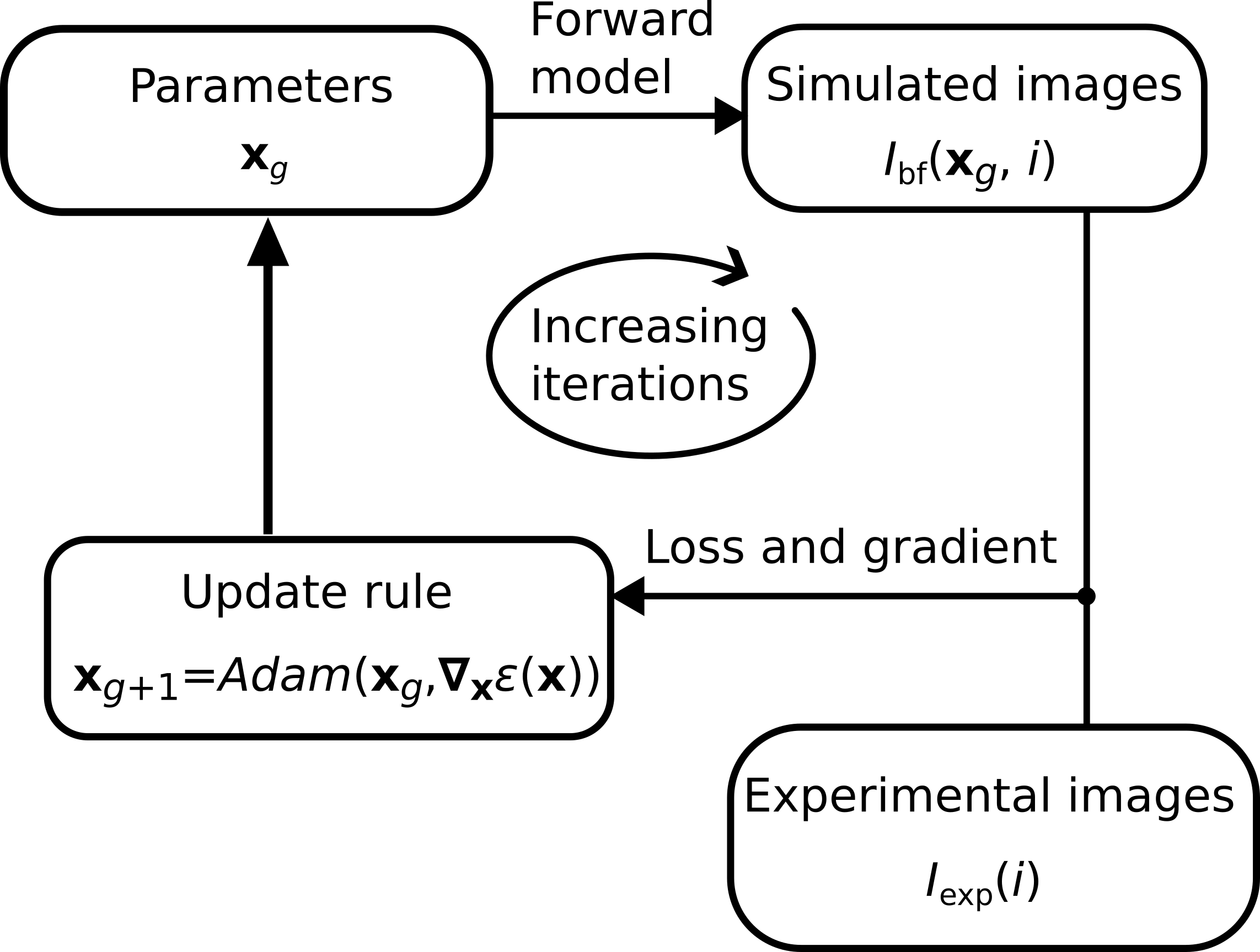
The goal of this algorithm is to iteratively solve for an unknown parameter vector, , that encodes the sample surface topography and strain. The surface geometry is represented by a mesh of control points defining a Bézier surface [56], which provides a smooth and compact parameterization suitable for gradient-based optimization (see Sec. S4 of the Supplemental Material). Given a trial parameter vector and a tilt angle , we compute simulated bright-field bend contour images and compare them to the corresponding experimental images . We quantify this comparison using a loss function
| (1) |
where is an image similarity metric, such as the mean squared error (MSE). Minimizing with respect to yields a best-fit estimate of the surface topography and strain. The optimization is performed using a gradient-based approach implemented in PyTorch [52], with parameters updated using the Adam optimizer [31]. Because our forward model is designed in a way that it is fully differentiable with respect to , gradients of the simulated intensities can be computed efficiently using automatic differentiation (see Sec. S7 of the Supplemental Material).
For the highly non-convex loss landscape, we employ a pyramidal optimization strategy to improve convergence, as demonstrated in scientific computing [61, 72], machine learning [12], and tomography [53]. In this approach, the reconstruction is first performed using a low-resolution Bézier surface with a small number of control points, allowing large-wavelength features to be captured efficiently. The optimized surface is then interpolated onto progressively finer control point meshes and re-optimized (see Sec. S4 of the Supplemental Material). This multiscale strategy significantly improves robustness compared to directly optimizing a high-dimensional parameterization.
Reconstruction of a freestanding oxide perovskite thin film

For experimental validation of BCET, we selected strontium titanate (SrTiO3), a perovskite oxide exhibiting incipient ferroelectric correlations. Although SrTiO3 avoids a ferroelectric phase transition at low temperature due to quantum fluctuations [47], it lies in close proximity to ferroelectric order. Perturbations including defects, interfaces, or reduced dimensionality can offset the energy landscape and stabilize polar distortions [64, 78, 77, 26]. In thin films, strong flexoelectric coupling further links strain gradients to polarization, enabling curvature-induced polar responses at the nanoscale [65]. Together with recent advances in freestanding oxide film synthesis [37], these properties make SrTiO3 an ideal platform for applying BCET to spatially resolve mesoscale strain fields.
We acquired a tilt series of electron micrographs on a room temperature 30-nm-thick SrTiO3 freestanding film using a 300 keV transmission electron microscope. A total of 40 images were recorded, rotating about two perpendicular tilt axes in a range of for each axis. A representative image at zero tilt is shown in Fig. 3(e); data at other tilt angles are shown in Fig. S7 of the Supplemental Material. Tilt series images were registered relative to each other using the underlying Cu mesh boundary. Bend contours in each bright-field image were manually masked by their diffraction order to generate virtual dark field images for constraining the direct solver, a manual step that took around four to six hours for the presented dataset but can potentially be automated via an artificial intelligence-assisted workflow (see details in Sec. S6 of the Supplemental Material). Based on the virtual dark field images, 298,572 constraints on the surface height map were formulated and supplied to the direct solver to reconstruct the surface topography. The corresponding bright-field image of the resulting surface is shown in Fig. 3(b), which is the initial guess for the subsequent iterative optimization.
For the iterative reconstruction, we employed a multi-phase strategy in which the number of free variables in was increased progressively. In each phase labeled by different colors in the loss curve [Fig. 3(a)], additional optimization parameters were introduced while previously optimized parameters were allowed to relax further. This hierarchical approach stabilizes the optimization and improves convergence by first fitting the most strongly constrained degrees of freedom before refining higher-order corrections. In the first stage, the pyramidal approach is utilized: increasing the control point number every 1,000 iterations starting from 10 10 to 20 20 after 4,000 iterations [Fig. 3(c)]; see Sec. S9 of the Supplemental Material for details on how we determined the best control point mesh size. In the blue, purple, and red regions of Fig. 3(a), tilt offsets, extra bend contour orders, and strain, respectively, are sequentially added to for optimization. Further details of the multiphase optimization procedure are provided in Sec. S8 of the Supplemental Material. After 13,000 total iterations, the reconstruction converges to a stable solution with quantitative agreement between simulated and experimental images [Fig. 3(d,e)]. Corresponding height and strain components of the converged solution are shown in Fig. 3(f,h–j). The reconstructed strain magnitudes are well above the strain sensitivity of approximately 0.1% granted by our experimental noise conditions (see details in Sec. S14 of the Supplemental Material). The effective resolution of this reconstruction is approximately 200 nm, estimated by the density of control points over the field of view. In total, the convergence of 1,279 parameters in was reached after less than 10 minutes using a single NVIDIA L40 graphics processing unit.
The mesoscale strain fields recovered here have direct physical consequences for SrTiO3. Its paraelectric-to-ferroelectric transition temperature rises steeply above zero with strain and can even reach room temperature or above at few percent level strains [22, 78, 36]. The 1–2% local strains revealed by BCET [Fig. 3(h–j)] are therefore comparable in magnitude to values shown to induce ferroelectricity in previous studies [78, 36]. Because this strain field is spatially heterogeneous, the film does not occupy a single point on the strain–temperature phase diagram but rather a continuous distribution of local states, with different regions of the film predicted to cross the ferroelectric phase boundary at different temperatures. Quantifying and visualizing this mesoscale strain landscape are precisely the class of questions BCET is designed to address. The resulting strain maps provide a quantitative structural foundation for interpreting the spatial organization of strain-driven phenomena, such as ferroelectric [36], magnetic [10], or even multiferroic orders [35, 71].
Validation
We validated the BCET algorithm along three axes: (i) identifiability analysis, which establishes that the inverse problem admits a unique solution given sufficient tilt data, (ii) subsampling cross-validation analysis, which quantifies the precision and stability of the reconstruction, and (iii) simulated reconstruction analysis under varying noise conditions, which evaluates accuracy.
A central concern for any inverse problem in tomography is whether the reconstructed solution is unique. In the case of BCET, local tilt and in-plane strain can be entangled as both factors enter the diffraction condition in a coupled fashion. A single bright-field image would underconstrain the inverse problem, in the same way that a single projection underconstrains a three-dimensional object in conventional tomography. To break the degeneracy between spurious and true solutions, we need to add independent constraints by tilting the sample, which can eventually yield a unique solution in an overdetermined inverse problem.
To validate the uniqueness of BCET, we relied on a general concept in optimization. For an underconstrained loss function, many local minima exist. Different starting parameters in the optimization procedure will result in uncorrelated and spurious solutions with a wide distribution of strain and height errors from the ground truth. On the other hand, if the solution is unique by including appropriate constraints, the loss function will fall into a single minimum. In this case, the algorithm will yield a narrow distribution of loss, strain errors, and height errors for different starting conditions. As detailed in Sec. S12 of the Supplemental Material, with a single tilt image, the converged loss, height, and strain errors are indeed broadly distributed, showing signs of a non-unique problem with many spurious solutions. As more tilt angles are included as input to the BCET algorithm, these distributions collapse to a tight, low-error cluster, marking the transition to a unique reconstruction. This transition is controlled jointly by the number of tilt images and the tilt range: what matters is that several non-parallel bend contours sweep across the full field of view while moving in small increments between adjacent tilts, so that each region of the freestanding film accumulates a sufficient number of constraints. As we show in Sec. S12 of the Supplemental Material, our experimental dataset (40 images over a tilt range) lies well inside this uniquely identifiable regime, and the same analysis indicates that comparably well-constrained reconstructions are achievable with far fewer images under an appropriately chosen tilt sampling.
In our cross-validation study to assess precision and stability of the BCET algorithm, we repeatedly run the final step of the multiphase reconstruction on random subsets of the experimental images. For each sampling fraction, we generate 40 reconstructions, each based on a newly selected data subset. If the algorithm converges to a consistent solution, the variation among the 40 reconstructions should be small compared to the mean value. Motivated by this intuition, at each sampling fraction, we computed the standard deviation across the reconstructed height and the three independent components of the strain tensors, shown in Fig. 3(g,k). After a sampling fraction of 0.5, the standard deviation among the 40 reconstructions of each strain tensor falls below the mean [see horizontal dashed lines in Fig. 3(k)]; for the height, the variation is way below the mean of 73 nm even at the smallest sampling fraction of 0.3. These observations indicate that the reconstruction is stable and converges to a consistent solution, independent of the specific subset of input images. More details of the precision validation can be found in Sec. S10 of the Supplemental Material.
To validate the accuracy of BCET, we performed reconstructions on simulated bend contour images with different noise levels and compared the result to the ground truth surface (see details in Sec. S11 of the Supplemental Material). Poisson-distributed shot noise, originating from the discrete nature of electron counting, was added to each pixel of the bright-field images. Dark current and read noise were omitted because they are insignificant relative to the shot noise under standard TEM conditions [76]. We varied the electron counts for the simulated shot noise from 1 to 10,000 at ten different values and used the iterative method to reconstruct the surface for each noise level. Figure 4(a–c) shows the simulated electron micrographs with different Poisson noise levels defined by the electron counts per pixel. For each noise level, we perform an iterative reconstruction and report the count-dependent initial and final loss, height MSE, and strain MSE in Fig. 4(d–f). The converged loss value is highly dependent on the noise level at all electron counts, but the height MSE plateaus near 100 electron counts at 0.1 nm2. The strain MSE reaches a relatively small value () at 100 electron counts, but continues to improve with electron counts. This behavior indicates that the algorithm maintains quantitative reconstruction accuracy down to approximately 100 electrons per pixel [Fig. 4(b)]. This level of electron count is well below the average experimental count of 8,200 electrons/pixel [see the vertical dashed lines in Fig. 4(d–f)]. These results demonstrate that BCET accurately recovers both surface topography and strain fields under realistic noise conditions.
Although we performed the experimental and validation studies on the high-symmetry cubic crystal of SrTiO3, reconstructing materials with a lower-symmetry space group does not introduce additional computational complexity or degraded performance. To demonstrate this capability, we performed reconstruction on a synthetic dataset of a monoclinic film of Ga2O3. Details can be found in Sec. S13 of the Supplemental Material.

Discussion
BCET relies on full-field acquisition rather than probe scanning, and therefore is uniquely suited for probing mesoscale structural heterogeneity with a large field of view up to hundreds of micrometers. This regime is difficult for typical scanning-based microscopy such as atomic force microscopy and scanning tunneling microscopy. Although BCET does not provide atomic resolution, it fills a critical gap between nanoscale probes and macroscopic optical microscopy methods. Importantly, BCET is uniquely suited for single-shot, ultrafast, and in-situ measurements for several reasons. First, eliminating the need for probe scanning minimizes the adverse effect of sample drift, making long-time data acquisition more robust. Second, BCET can be implemented on virtually any conventional TEM setup and it does not need a specialized tomography sample holder. Third, the relatively small amount of data needed for reconstruction compared to scanning nanobeam electron diffraction and other data-intensive methods makes it possible for efficient or even real-time data processing. Furthermore, the computational framework introduced here can be straightforwardly extended to accommodate a large number of additional parameters in , especially in light of the rapid advances and widespread availability of parallel computing today. These attributes establish BCET as a broadly accessible approach for resolving complex structural landscapes in crystalline thin films, which also provides a versatile platform for studying flexo-ferroic coupling, thin film acoustic excitations, and emergent functionality arising from strain gradients in freestanding membranes [28, 75, 64].
Several technical extensions can further expand the scope and impact of BCET. By measuring bend contours beyond the first Laue zone, the same framework can be used to recover the spatial map of out-of-plane strains that typically have the fastest response following photoexcitation by a femtosecond laser pulse [14]. We demonstrate this possibility using a synthetic dataset in Sec. S15 of the Supplemental Material. Incorporating film surface models that fit multi-domain crystalline regions using a piecewise continuous function would enable quantitative mapping of crystallographically heterogeneous systems using BCET. This capability would allow direct visualization of domain switching or even topological defect motion, which play a central role in nonequilibrium phase transitions [13]. Furthermore, applying BCET to reconstruct more intricate surface geometries, such as folded sheets or patterned membranes exemplified in kirigami structures [6], would make it possible to directly visualize the strong strain localization and pronounced curvature that develop along folded creases or cut features [67]. These capabilities would establish BCET as a powerful tool for resolving complex mesoscale structural landscapes that remain difficult to quantify with existing techniques.
By reconstructing surface topography and the full in-plane strain tensor, BCET enables direct visualization of strain gradients and curvature that underlie higher-order electro- and magneto-mechanical couplings [64, 28]. These effects are particularly sensitive to mesoscale structural heterogeneity, including bending, wrinkling, and local curvature variations common in freestanding thin films [25, 20, 39, 27]. BCET therefore provides a quantitative structural framework for operando investigation of emergent phenomena in low-dimensional materials driven by strain and nontrivial topography. Our work further illustrates how combining a widely accessible full-field imaging technique with modern parallel computational architectures offers a powerful strategy for quantitative microscopy.
Acknowledgments — We thank helpful discussions with Cedric Lim, Patrick Liu, and Jared Maxson. We thank Andrew Barnum and Pinaki Mukherjee for assistance with the TEM measurements. We thank Jiarui Li for SrTiO3 characterization. C.O. acknowledges funding support from the DOE Office of Science FWP-101256, Enabling Science for Transformative Energy-Efficient Microelectronics. H.Y.H and M.H. acknowledge funding from the U.S. Department of Energy, Office of Basic Energy Sciences, Division of Materials Sciences and Engineering, under contract No. DE-AC02-76SF00515. A.Z. and H.G.B. acknowledge the support from the U.S. Department of Energy, Office of Basic Energy Sciences under award No. DE-SC0026202. Part of this work was performed at nano@stanford (RRID:SCR_026695), and we thank the C-ShaRP Voucher Program for supporting the facility access.
Supplemental Material to “Bend Contour Electron Tomography (BCET):
Quantitative strain and topography mapping”
Henry G. Bell, Chenhang Xu, Arthur McCray,3 Minyong Han,1, 2
Yicheng Zhuang,4 Harold Y. Hwang,1, 2 Colin Ophus, and Alfred Zong
†† ∗These authors contributed equally: H.B. and C.X.†cophus@stanford.edu (C.O.) and alfredz@stanford.edu (A.Z.)
1Department of Applied Physics, Stanford University, Stanford, CA 94305, USA
2Stanford Institute for Materials and Energy Sciences, SLAC National Accelerator Laboratory, Menlo Park, CA 94025, USA
3Department of Materials Science and Engineering, Stanford University, Stanford, CA 94305, USA
4Geballe Laboratory for Advanced Materials, Stanford University, Stanford, CA 94305, USA
5Department of Physics, Stanford University, Stanford, CA 94305, USA
S1 Thin film surface parameterization
In this section, the mathematical foundation of bend contour electron tomography (BCET) will be laid out in terms of thin film surface parameterization, local lattice information, and strain tensor derivation. A thin film can be represented by a 2D surface embedded in 3D space, . Here, are parametric surface coordinates. Both the height and strain information are contained in this mathematical description. To compute the local lattice vectors, we first compute the tangent vectors, , given by,
| (S1) |
These vectors are normalized not by their local amplitude, but by global amplitudes, , to retain the strain information. These global amplitudes are calculated based on a flat reference configuration surface. We can now define a local coordinate system captured by a coordinate matrix, , given by
| (S2) |
Here, is a unitary surface normal vector . More generally, the surface normal vector need not be a unit vector if out-of-plane strain is present. Here, we focus on in-plane strain, so we are only concerned about the unit vector ; the case for out-of-plane strains is considered in Sec. S15. The matrix defines a coordinate system at each point on the surface with the tangent and normal vectors.
The real space lattice vectors at each local coordinate are readily computed from the columns of a related matrix , defined as
| (S3) |
where the columns of the matrix are the real space lattice vectors, [see Fig. S2(a)], expressed in an arbitrarily chosen reference frame of the material system. The matrix, , is a global rotation matrix that transforms the lattice vectors into the experimental reference frame, and it allows for the situation where is not necessarily parallel to . The reciprocal lattice vectors, , , are then the columns of .
To compute the in-plane strain of a given surface function, nonlinear strain theory is used [24]. The undeformed configuration, , is defined as a flat surface with for all coordinates, where is the identity matrix. The deformed configuration is the surface function, . The linear transformation from the reference frames of the undeformed configuration to the deformed configuration is the deformation gradient tensor, , defined as
| (S4) | ||||
| (S5) |
The deformation gradient tensor encompasses the rotational, shear, and scaling transformations from the frame of the undeformed reference surface to the frame of the deformed surface. To remove the rotational components of the deformation gradient, the right Cauchy strain tensor can be found with
| (S6) |
The Green-Lagrange strain tensor is then computed with
| (S7) |
The in-plane portion of this tensor is used as the metric of strain in the BCET algorithm.
S2 Bend contour as an approximate iso-gradient contour

Bend contours can be thought of as the location on the film where the diffraction condition is met, but this misses a key insight into why this contrast forms 1D contours on a continuous crystalline surface. Here we introduce a more concrete mathematical description of bend contour contrast which can explain this intrinsic feature. For the diffraction condition to be met, the reciprocal lattice vector, needs to be elevated from the plane perpendicular to the incident electron wavevector, , into the Ewald sphere by the Bragg angle, [Fig. S1(a)]. In a surface with curvature or strain, is a function that depends on the position on the surface, . As shown in Fig. S1(a), the diffraction condition of can be expressed as
| (S8) |
where is the Bragg angle. Using Bragg’s law,
| (S9) |
we get the bend contour condition,
| (S10) |
At any coordinates where Eq. (S10) holds, the diffraction condition is met and bend contours will be observed. Graphically, both the left and right hand sides of Eq. (S10) define a 2D surface parameterized by for a given order. The intersection of two 2D surfaces therefore results in a 1D contour. If is a smooth surface, we expect both left and right hand sides of Eq. (S10) to be smooth surfaces of . Under this condition, the resulting bend contour is a continuous 1D curve, which either forms closed loops or terminates at the edge of the domain.
Let us gain some intuition about the left and right hand sides of Eq. (S10). The term on the left hand side is computed based on a linear transformation of the vectors defining the tangent plane at . Hence, we can view as some generalized gradient of the surface at projected into specific directions as defined by the Bragg order and the incident electron direction . We will henceforth call generalized gradient. As for the right hand side of Eq. (S10), in the special case of zero strain, it becomes independent of , so we can define
| (S11) |
which are simply horizontal planes in the coordinates.
The graphical solutions to the bend contour condition in Eq. (S10) in the zero-strain case are visualized through Fig. S1(b–e). For the SrTiO3 film surface shown in Fig. S1(b), we compute the generalized gradients for four peaks [see Fig. S1(c)]. For the right hand side of Eq. (S10), constant height surfaces are drawn at values for each triplet [see peak selections in Fig. S1(d)], where is an integer. Here, is needed because the term in Eq. (S10) is a unit vector, so all are identical. Finally, bend contour contrast of the order is present at the intersection between the two surfaces defined by the left and right hand sides of Eq. (S10), as plotted in Fig. S1(e). In this case, bend contours can be understood as constant-height contours of the generalized gradient, i.e., iso-gradients.
The left hand side of Eq. (S10) for the bend contour condition also points out two important invariants. Because the left hand side only depends on the relative angle between the incident electron direction and the reciprocal lattice unit vector , the bend contour position will be unchanged under a global rotation of the crystal if the rotation axis is or . More specifically, if the crystal rotates around , bend contours of all orders remain unchanged in their locations. If the crystal rotates around , all bend contours remain unchanged. These properties are useful when we construct the direct solver, as explained in more detail in Sec. S5.
Moving beyond the trivial case of zero strain, we can also consider the special case of a spatially homogeneous in-plane strain. In this case, the generalized gradient on the left hand side of Eq. (S10) remains unchanged, while the right side will be scaled linearly by the strain magnitude depending on the strain direction relative to the local direction. The isocontour planes in Fig. S1(d) will remain flat and horizontal, but their vertical spacing will contract (or expand) with tensile (or compressive) strain. In the most general case where the in-plane strain is spatially inhomogeneous, the right hand side of Eq. (S10) is no longer a constant function of . The bend contours no longer occur at a constant height in Fig. S1(d), but can still be defined as the intersection of two surfaces.
Tilting the sample, which is commonly done in experiment, will add a -independent constant to , where the constant depends on the tilt axis and angle. The right hand side of Eq. (S10) will be unchanged. Rotation of the sample will therefore vertically displace the curved surfaces in Fig. S1(d), changing their intersection with the planes, which will smoothly move and change the shapes of the contours.
Fundamentally, bend contours can be formulated as the intersection of two surfaces. With small strain fields, they can be thought of as constant height contours of the generalized gradient surface, .
S3 Forward model details

In this section, we describe the computational procedure by which the bend contour images are generated, namely, the forward model. We compute the TEM diffraction intensity by considering the excitation error, , which is the minimal momentum-space distance from to the Ewald sphere surface [76]. We compute as
| (S12) |
Due to the finite volume of the reciprocal peak and the finite thickness of the Ewald sphere, bend contours must have a finite width. We model these considerations by computing the dark-field bend contour intensity using a Gaussian function with width ,
| (S13) |
We chose a Gaussian over a more theoretically motivated sinc function [76] because Gaussian is numerically efficient to evaluate and does not significantly change the simulated bend contour images in our thickness range. An example excitation error map and dark-field intensity map are shown in Fig. S2(c,d). At the locations where the excitation error reaches , the dark-field intensity evaluates to .

We next compute the bright-field intensity map,
| (S14) |
Here, are all possible Miller indices up to a cutoff depending on the tilt of the sample; in addition, the case of is excluded in the sum. is a global adjustment to match the experimental electron counts and is a constant background offset due to factors such as the detector dark current. is the complex structure factor based on the kinematic diffraction theory while is an order-dependent normalization factor that also accounts for effects such as multiple scattering.
It is worth emphasizing that the quantitative outputs of BCET, including the surface topography and in-plane strain tensor, are not encoded in the intensity of bend contours but in their positions, namely, the loci in where the excitation error vanishes [, see Eq. (S12)]. The intensity-related quantities in the forward model, such as the Gaussian width [Eq. (S13)], the order-dependent amplitude [Eq. (S14)], and the global scale [Eq. (S14)], act only to match the appearance of the contours and are treated as free nuisance parameters that are fit alongside other reconstruction parameters. Effects that redistribute or rescale diffracted intensity, including dynamical and multiple scatterings, thickness inhomogeneity, and partial beam coherence do not bias the reconstructed morphology and strain because they do not displace the contour positions even though they can modify contour contrast and width.
S4 Bézier surface parameterization

For iterative optimization, using the pixel basis of the surface, which would involve optimizing each point in , becomes intractable in terms of memory use and computational time for high-resolution TEM images. Instead, a different surface parameterization is needed. We found inspiration from computer graphics to use Bézier surfaces as our surface description [56]. In this representation, control points define a 2D mesh in 3D space. The surface function can be found with
| (S15) |
which interpolates a smooth surface through the control points with arbitrary -, -resolution. The functions are Bernstein polynomials defined as,
| (S16) |
For our application, Bézier surfaces are useful for a few reasons stemming from the observation that transformation from control points to surface coordinates is linear. For example, a matrix can be created that linearly multiplies the control point coordinates to retrieve the surface coordinates,
| (S17) |
Here, the indices of are flattened to a single index for computational convenience. Similarly, the control point indices are flattened into an index . is computed with
| (S18) |
This linear relationship enables the pyramidal optimization strategy. After convergence is reached for one mesh size during pyramidal optimization, we need to find a higher resolution control point mesh that produces the same surface as the lower resolution control point mesh. To find an optimally matched surface with control points instead of control points, we can equate the surface coordinates,
| (S19) |
This is a linear constraint that can be efficiently solved with least squares. As explained in Sec. S5, we will also use this linear transformation property in the direct solver, where this transformation matrix multiplies the constraint matrix, enabling us to solve for the control point mesh rather than the surface pixel coordinates.
S5 Direct solver details
In this section, we will explain the constraints used in the direct solver for a fully general unit cell. This constraint has to be carefully constructed to be linear in the surface height pixels, , so we can solve it with least squares. Here, () are the discrete integral indices for the continuous parameterization coordinates (), and as before, the flattened indices of is denoted by . Here, is used to describe the surface height because without strain, it is a simpler parameterization of the surface than .
Generally, we want to formulate constraints that can be described in the form of
| (S20) |
where is the flattened height vector over the 2D surface, is some vector, and is a scalar, which together describe a general linear constraint on . This constraint formulation from bend contour contrast is nontrivial to devise because the reciprocal lattice vectors are a nonlinear function of the surface height. However, the surface normal unit vector,
| (S21) |
can be linearized in the limit of small ripple amplitude. Therefore, we formulate the diffraction condition as a constraint on the normal vector.
Let us first review the discussion in the main text, where in the absence of strain and in the special case of a cubic lattice system, a convenient constraint to use for the observation of a bend contour at is,
| (S22) |
where we know that intersects with the Ewald sphere; by assuming one global in-plane rotation, can be uniquely determined. We can solve for the normal vector from the height map with the cross product between two non-parallel vectors in the tangent plane to find,
| (S23) |
where , , are the unit vectors in the Cartesian coordinate directions and
| (S24) | ||||
| (S25) |
Here, and are the scalings from to real space Cartesian coordinates on the grid. The constraint from Eq. (S22) in the matrix form reads
| (S26) |
For general space groups, Eq. (S26) does not always hold true. The general constraint can be formulated as a fixed angle between and , where the angle is not necessarily . This constraint can be understood from the conditions for diffraction and bend contour formation: when the crystal is rotated around , the diffraction condition for that order is unchanged. To formulate the general equation for this constraint based on the height map, we must find the constant angle, denoted by , between and . Let us first define the three angles, , and as,
| (S27) | ||||
| (S28) | ||||
| (S29) |
To find , we compute the dot product between and , yielding
| (S30) |
where we utilized the relation in Eq. (S21). Here , , and . As a sanity check, if and , we retrieve the expected result of .

We are now ready to formulate the general constraint on the height map, . We first find the unit normal vector,
| (S31) |
In the limit where , we find that is approximately equal to in Eq. (S23). This is true when the slope of the wrinkles in the thin film is much less than 1. Although higher-order terms could be retained for larger slopes, the small-slope approximation ensures linearity, making the reconstruction tractable via linear least-squares. The general constraint then becomes,
| (S32) |
Coming back to our original goal to constrain the surface, for each dark-field pixel, for a certain order , we find the vector that intersects with the Ewald sphere, and has the assumed in-plane rotation. Then, we rewrite Eq. (S32) in the form of for efficient linear computation, where and can be directly derived from . These constraints are stacked into a matrix and as a whole can be written as
| (S33) |
Here, the dimension of is the number of constraints by the number of pixels in , and is a vector of stacked ’s with length equal to the number of constraints.
As mentioned in Sec. S4, we do not need to solve all the constraints in the pixel basis, . Instead, we can solve it in the Bézier basis, which provides a few key advantages. Using the coordinate of Eq. (S17), we can rewrite as
| (S34) |
where is the coordinate of the control point mesh. The direct solver constraint then becomes,
| (S35) |

Solving Eq. (S35) has the added computational advantage over solving Eq. (S33) because the number of control points is usually orders of magnitude fewer than the number of pixels. Using the Bézier solution basis also has the implicit benefit of providing regularization because Bézier surfaces are naturally smooth.
To validate the direct solver, we performed a simulated reconstruction on an example surface without strain. The ground truth height of a known analytic surface function and the corresponding bright-field image from the forward model are shown in Fig. S4(b,g). We enforced the direct solver constraints on the hot pixels of the thresholded simulated dark-field images, and solved the resulting matrix in the Bézier basis. The resulting height and bright-field images are shown in Fig. S4(c–f) and (h–k). We computed the mean squared error (MSE) of the height for each control point mesh and report the result in Fig. S4(a). We observe an underfitting range from 2 2 to roughly 10 10 control points, followed by a wide appropriate fitting range from 10 10 to 25 25 control points, and an overfitting regime above 25 25 control points.


S6 Dark field labeling
For the input to the direct solver, we must know the order of each bend contour. A straightforward way to achieve this task is to perform dark-field mapping of all peaks at each tilt. While possible, in practice it becomes unrealistic to do this. Instead, while acquiring a bright-field tilt series, we performed dark-field mapping only when unknown bend contours appear upon tilting. In this modality, some post processing is required. In particular, manual image labeling is performed on each tilt series image to assign each contour to an triplet based on the slow continuous deformation of the bend contours during sample rotation and comparing known bend contour orders from a previous tilt. In Fig. S5, an example manual labeling is shown for the SrTiO3 sample area, which is reconstructed in this work. We labeled six contour orders from the bright-field images, resulting in masks which we used to create virtual dark-field images. The masking itself is facilitated by standard interactive segmentation tools. In our workflow, we used an open-source data-labeling tool called Label Studio [73]. This tool provides brush/polygon selection and propagation of labels between adjacent frames, which substantially reduce the per-image effort relative to labeling from scratch.
Two types of errors may occur during manual labeling. First, the order of a bend contour may be mislabeled, but such errors are easy to verify by checking the consistency between labels in nearby tilts and are thus not a primary concern. Second, the exact shape of the mask may not be consistent across different label trials. However, because the direct-solver constraints are derived from a skeletonized, single-pixel-wide representation of each virtual dark field image rather than the exact mask boundary (see Sec. S8), the solver is relatively insensitive to the precise shape of the manual mask. Furthermore, this manual labeling step only informs the direct solver, and therefore only informs the initial conditions of the BCET iterative reconstruction. While this labeling is an important and required step, the final converged solution is not sensitive to small variations of the initial conditions.
We recognize that the labeling step is the principal manual bottleneck of the direct solver, but automation is possible given rapid advances of automated and autonomous experimentation in (S)TEM, with demonstrations of self-driving microscopes that autonomously navigate image space, correct aberrations, and select acquisition targets under varying conditions [60, 29]. In our context, the two automatable pieces are (i) acquisition of the dark-field tilt series used for order cross-referencing, which fits naturally within existing self-driving TEM frameworks, and (ii) contour masking and order assignment, for which the continuous frame-to-frame deformation of contours makes propagation-based tracking and learned segmentation well suited.
S7 Iterative optimization loop
For the iterative method, a computational loop is evaluated at each iteration to minimize the loss, in Eq. (1). This loop is shown in Fig. S6. First, the parameters , which consists of the surface control points and geometric/experimental parameters where is the iteration count, are sent through the forward model to compute the bright-field images . The index denotes the different tilt angles. Simulated images are then compared with the experimental images with MSE to form the loss function. We tried multiple image similarity metrics, such as cross correlation, but we chose MSE based on a good balance between simplicity and performance. The loss gradient is efficiently computed with a backpropagation step through the computational graph, which is implemented with automatic differentiation in PyTorch [52]. The gradients are used to descend the loss landscape with the Adam update rule [31]. After a fixed number of iterations, we terminate the optimization loop. The loss and parameter stability is then evaluated to see if the solution is converged. Hyperparameters such as Adam learning rates were manually adjusted based on multiple simulated and experimental reconstructions, balancing speed and successful convergence.
S8 Experimental reconstruction details
In our experiment, we employed an FEI Titan TEM with 300 keV acceleration voltage at a magnification of 1750. We employed a Gatan K3 direct electron detector to capture 4K resolution bright-field images. We collected 1 s exposure bright-field tilt series images of a freestanding 30-nm-thick SrTiO3 film on a 2,000 mesh copper TEM grid (see Sec. S16 for sample preparation details). We used a double-tilt holder with angles , where the tilt axes are perpendicular to each other. See Fig. S9(a) for the experimental geometry and Fig. S7 for example bright-field images. We performed the tilt series by fixing one of the angles and rotating the other, with steps from to in each direction. During the tilt series, we employed dark-field mapping if new bend contours appeared, and performed manual dark-field labeling as described in Sec. S6.
For the direct solver, the virtual dark-field images were sent through a skeletonize image filter [74] to extract the single pixel-thick central bend contour line as a binary image. Each nonzero pixel is converted to a constraint and solved with the direct solver (see Sec. S5). We solve for the Bézier surface control points in the Cartesian basis, , where , and , are parallel to the image axes. For the input to the direct solver, the relationship between the image pixel axes, the rotation axes, and the image scale must be approximately known, as well as the global in-plane rotation of the reciprocal space vectors. In our case, the order peaks do not move significantly with , even up to rotations of , allowing us to ascertain that the rotation axis is approximately parallel to the vector. Additionally, we use the known shape of the cylindrical hole in the TEM grid, as well as the projected intensity through the hole at the largest accessible tilt angle () to approximately determine the axis. The image scale is determined by the known diameter of the 2,000-mesh TEM grid. Using the constraints from the virtual dark-field images, and the described sample/tilt holder geometry, we use the direct solver with a control point grid to solve for the surface topography in the absence of strain. The resulting surface and example bright-field image are shown in Fig. S8(a,b). Comparing the direct solver result and the corresponding experimental image [Fig. S8(b,c)], the direct solver indeed yields a reasonable guess as an input for the iterative solver.
For the iterative solver, the surface solution from the direct solver in Fig. S8(a) is used as a starting point. In practice, the circular field of view is cropped to an inner square, which streamlines the convergence for the iterative solver. Additionally, parameters like the peak width () and global intensity () are manually selected to match the bright-field image, which act as the initial guess for the iterative solver. These parameters are then refined with the iterative method.

In particular, for the multiphase optimization shown in Fig. S9(b), in the first region (green), the peak intensity adjustment of the dominant bend contours is optimized, and so is the Gaussian width (), in-plane crystal axis rotation (), and the rotation axis (). The axis is fixed to be perpendicular to the axis [see the experimental geometry schematic in Fig. S9(a)]. In this first region, the control point mesh number is slowly scaled up from to using the pyramidal method, as decided from the leave-half-out cross validation procedure described in Sec. S10, where the cross validation is minimized at 20 control points [Fig. S10(a)].
In the second (blue) region of Fig. S9(b), tilt offsets in are relaxed, which are included because of inherent error in the reported angle of the rotation stages in the TEM. For example, we observed that in two bend contour images taken at the same reported angles tens of minutes apart, the bend contours are translated with respect to each other, indicating a drift in the reported tilt angle. The optimized values of tilt offset stay within roughly without any constraint.
In the third (pink) region of the multiphase procedure in Fig. S9(b), 50 more peaks are added from and . Due to computational speed considerations, only the peaks that contribute intensity to the bright-field images are included. The initial intensity adjustment of these peaks is chosen to be 0, constrained to be the same value for symmetrical , and refined through iterative optimization. In the final region, the strain is relaxed, meaning that the control points in the Bézier parametrization are allowed to move laterally, in and .
S9 Determination of the optimal number of Bézier control points for the iterative reconstruction

In this section, we use cross validation [32, 3] to decide the optimal number of control points. This approach generally relies on repeated random sub-sampling of the experimental images, performing independent reconstructions from different data subsets, and comparing the resulting solutions.
Before applying cross-validation to determine the optimal number of control points, it is important to consider the bias–variance tradeoff associated with model complexity. Increasing the number of control points improves the ability of the model to resolve fine spatial features, but also increases sensitivity to noise and the risk of overfitting, resulting in higher variance. Conversely, using too few control points limits the expressive capacity of the model, leading to underfitting and increased bias. This tradeoff implies that an intermediate number of control points exists that balances model flexibility and stability, providing an optimal representation of the surface.
To find this control point mesh size, we performed a leave-half-out cross validation strategy. In particular, starting from the same initial , we split the available data into two halves that are randomly sampled, and we performed a reconstruction on each half separately. This procedure is repeated multiple times, and the final strain distributions are compared between reconstructions. High variance in the reconstructed strains using different data would suggest either under- or over-fitting to the data, while minimum variance suggests appropriate fitting. By repeating this procedure for a different number of control points, the optimal control point number can be surmised. In this case, because we are confident in the height map results, we start our cross validation from the converged result of the optimization without strain.
We performed leave-half-out cross validation with control point mesh size from to , with 40 reconstructions at each control points number. The cross validation metric, chosen to be the standard deviation of the strain over reconstructions, averaged over the surface, is plotted in Fig. S10(a). The plot shows a standard cross-validation behavior: with a low number of control points, we are not able to accurately capture the experimental data, and we are therefore underfitting, resulting in higher strain variance. If we use too many control points, the surface will overfit to the data subset and we will again see high strain variance. We find a minimal cross validation standard deviation of at (i.e., 2020 grid). Therefore, we use this control point number in the final reconstruction.
S10 Assessing the reconstruction precision
In order to evaluate the precision of our reconstructed solution in the absence of the ground truth, we performed a related cross validation sub-sampling analysis as in Sec. S9 but instead of varying control point number, we use a variable sampling fraction. Namely, we choose a sub-sample of the tilt series images with sampling fraction from 0.3 to 0.975. At each sampling fraction, we perform 40 reconstructions with independent datasets. The variability among these reconstructions at a given random sampling fraction provides a quantitative basis for selecting the optimal regularization parameter and evaluating the statistical precision of the reconstruction.
In Fig. S10(b–g), we provide the scaling of the cross validation error with variable sampling fraction and a fixed control point number for a select collection of optimized parameters. To assess the precision of the reconstructed parameters in Fig. S10(b–g), we evaluate the cross-validation standard deviation at the largest sampling fraction, which provides the closest estimate of the statistical precision of the final reconstruction. For parameters with physically meaningful absolute magnitudes like strain or height deviation, the cross-validation standard deviation can be compared directly to the characteristic parameter value to assess statistical significance. For example, for the strain, the cross validation standard deviation falls below the mean deviation magnitude at a sampling fraction of [see the shaded region and circular markers in Fig. S10(g)], indicating a statistically meaningful result for our reconstruction. For the height in Fig. S10(f), the cross validation standard deviation is on the order of 1 nm, which is well below the mean height near 73 nm. For parameters with arbitrary reference offsets, such as global orientation angles, precision can only be quantified in absolute terms. In our case, angular parameter cross validation standard deviation values are less than , indicating a stable reconstruction that is well constrained by the data.

S11 Assessing the reconstruction accuracy
To assess the accuracy of the BCET method, we performed a validation using simulated data from a known ground truth surface. Specifically, we defined an analytical surface geometry, simulated the corresponding bend contour bright-field images, and applied the BCET reconstruction algorithm to recover the surface and strain from these images. The reconstructed surface was then directly compared to the ground truth to quantify reconstruction accuracy. The ground truth surface was defined by the analytical function below, with characteristic length scale ,
| (S36) | ||||
| (S37) | ||||
| (S38) |
where are chosen constants and
| (S39) |
The term produces the tensile/compressive strain centered at . The bright-field images from this surface were simulated at a 10∘ clockwise rotation angle from the axis, with 20 tilt series images from to in a single tilt axis. A selected image at zero tilt is shown in Fig. S11(g). To test the limits of the inverse solver, we use a starting guess surface that is generated from a combination of analytical functions with zero strain,
| (S40) | ||||
| (S41) | ||||
| (S42) |
This starting guess is significantly further from the ground truth than what the direct solver provides. To start the optimization, the functions in Eqs. (S40)–(S42) were fit with control points using Eq. (S17) to define the initial control point mesh. The initial geometric parameters such as rotation, width, in-plane rotation were set slightly off their ground truth value. We sent this initial guess through the iterative optimization loop 5,000 times, resulting in the reconstruction in Fig. S11.
Unlike experimental reconstruction, we now have access to the height MSE and strain MSE [Fig. S11(b,c)], which reach extremely small values. In both simulated and experimental cases we have access to the loss, which is shown in this case in Fig. S11(a). The parameters such as peak width, tilt axis, and in-plane lattice angles over optimization can be seen in [Fig. S11(d–f)], which converge to their ground truth values. The surface height, strain and bright-field images closely match the ground truth [Fig. S11(g–j)].
In Fig. S12, we display the surface height maps [Fig. S12(a)] and bright-field images for different iteration counts [Fig. S12(b)]. The Bézier surfaces quickly approach the ground truth with reasonable agreement after only 100 or 200 iterations, but their bright-field images differ significantly, showing the large sensitivity of bend contour contrast to the topography/strain.
Next, interested in the scaling behavior of the BCET algorithm with experimental noise, we augment all bright-field pixels with Poisson noise due to electron counting statistics. In particular, we augment each pixel value by applying Poisson counting statistics,
| (S43) |
Here, is the normalized original pixel value so that it falls in the range of , denotes a Poisson random variable with mean , is the electron counts per pixel, and is the resulting pixel value. By performing the same simulated reconstruction as described in this section but for variable , we demonstrate the robustness of BCET against realistic experimental noise conditions; see Fig. 4 and the accompanying discussion in the main text.
S12 Assessing the reconstruction uniqueness
Any inverse-problem approach to structural reconstruction raises the question of whether its solution is unique: whether the experimental data is sufficient to select a single surface and strain field, or whether many distinct configurations reproduce the same bend-contour images equally well. The local tilt and in-plane strain enter the bend-contour condition [Eq. (S10)] in a coupled fashion, so that a single bright-field image underconstrains the problem. The degeneracy is broken by acquiring images across a range of tilts, but the minimum amount of tilt data required to reach a unique solution is not obvious a priori. In this section, we develop an empirical test for assessing reconstruction uniqueness and use it to quantify how the reconstruction fidelity depends on the number of tilt images and the total tilt range.
S12.1 An empirical identifiability criterion


Because our forward model is nonlinear and the loss landscape is non-convex, we assess uniqueness empirically rather than analytically. The key idea, sketched in Fig. S13, is that a unique, well-posed reconstruction corresponds to a loss landscape with a single dominant minimum, so that independent optimizations started from different random initial conditions all converge to the same solution. A non-unique reconstruction, by contrast, possesses multiple loss minima of comparable depths, and random restarts scatter across distinct solutions with widely varying ground-truth errors [Fig. S13(a,b)]. This distinction produces a directly observable signature: in the non-unique case, the final loss and the ground-truth error are both broadly distributed across restarts, and a low final loss does not guarantee a small error because the optimizer may have settled in a spurious minimum [Fig. S13(c)]. In the unique case, both quantities are tightly concentrated, and a low loss reliably implies a low error [Fig. S13(d)]. Crucially, this criterion can be evaluated without knowing the true solution and without constructing a specific competing configuration: the spread of outcomes across random restarts alone diagnoses the transition from the non-unique to the unique regime. When a ground-truth surface is available, as in the simulated tests below, we additionally verify that the concentrated-loss regime coincides with a small ground-truth error.
S12.2 Dependence on the number of tilt images

We first applied this criterion to determine how many tilt images are needed for a unique reconstruction for a fixed tilt range. Using the simulated ground-truth dataset of Sec. S11, we performed 25 independent reconstructions from randomly sampled starting points for tilt series of 1, 10, and 20 images spanning the same angular range, and recorded the final loss, height RMS error, and strain RMS error for each restart. The resulting distributions are shown as box plots in Fig. S14. With a single tilt image [Fig. S14(a)], all three quantities are broadly distributed across the 25 restarts, the signature of a non-unique loss landscape in which many distinct height–strain combinations are compatible with the limited data. At 10 images [Fig. S14(b)], the distributions narrow appreciably but retain noticeable variance. By 20 images [Fig. S14(c)], the loss, height error, and strain error all collapse to tight distributions across every restart, indicating that the reconstruction has entered the unique regime: the data alone select a single solution, independent of initialization. Our experimental SrTiO3 dataset of 40 images therefore lies well within this unique regime, providing a substantial margin of overdetermination relative to the transition.
This behavior can be understood intuitively by counting how many bend-contour constraints fall on each pixel in the field of view as the tilt series grows. Figure S15(a–c) shows spatially-resolved maps of the number of bend contours passing through each pixel, accumulated over 1, 10, and 20 tilt images, with the corresponding histograms in Fig. S15(d–f). With a single image, the majority of pixels are traversed by no bend contour at all, leaving the surface largely underdetermined [Fig. S15(a,d)]. As the number of images increases, the bend contours sweep across the field of view, the zero-constraint population shrinks, and pixels progressively accumulate constraints from multiple nonparallel orders [Fig. S15(c,f)]. At 20 tilt images, the majority of the surface is constrained, with small regions having zero constraints. These regions can still be reliably reconstructed with surface smoothness regularization given by the Bézier parameterization.
S12.3 Dependence on the tilt range

The total angular range spanned by the tilt series also determines identifiability. To isolate its effect, we repeated the restart analysis at a fixed image count, performing 25 independent reconstructions for tilt ranges of , , , and , each with 20 images distributed uniformly across the range. To mimic a double-tilt holder, 10 images were acquired by varying at fixed , and 10 by varying at fixed . The resulting distributions of loss, height RMS error, and strain RMS error are shown in Fig. S16. At the smallest ranges, and , all three metrics are broadly distributed across restarts, indicating that the limited angular variation provides insufficient constraint to distinguish between distinct surface and strain configurations. By , the distributions collapse to narrow bands, and they remain tightly concentrated at , showing that the reconstruction has entered the unique regime. The full range with 40 images used in our experiment thus provides a comfortable margin above this threshold.
The qualitative difference between the non-unique and unique regimes is made explicit in Fig. S17, which compares representative reconstructions at and tilt range. At , the reconstructed bright-field image is visually plausible for a large part within the field of view [Fig. S17(a)], yet the recovered height and strain maps are inconsistent with the ground truth, with an RMS height error of nm and an RMS strain error of [Fig. S17(b,c)]. The strain map of , in particular, shows unphysical, sharply varying features. At , the same reconstruction procedure recovers smooth, physically meaningful height and strain fields with RMS errors of nm and [Fig. S17(e,f)].


As with the image-count analysis, what is important for identifiability of the inverse problem is the number of constraints gained from the tilt series. In Fig. S18(a–d), we plot the number of bend contours that traverse each pixel. At the tilt range, many large regions of the surface do not have any bend contours, noted by the red pixels. This lack of constraints leads to an unreliable reconstruction. For higher tilt ranges, more bend contours traverse the field of view, and the constraints are more evenly distributed, leading to a constrained surface. It is clear from Fig. S18(a–d) that a tilt range of is approximately ideal for this example surface because the bend contour constraints cover almost the entire surface, with a large swathe of the surface constrained by more than one contour [Fig. S18(g)]. By a tilt range of , the surface is relatively less constrained because the tilt step is too large; bend contours move large distances between tilts, again leading to some unconstrained regions. In an experiment, one can choose the minimal tilt range and number of images by making sure a few non-parallel bend contours traverse the entire field of view, and that the bend contours do not jump large distances between nearby tilt images in order to get a well-constrained solution.
S12.4 Minimum image number required for unique reconstruction and implications on ultrafast TEM
Whether a BCET reconstruction is well-constrained is governed jointly by the tilt range and the number of images. While choosing the tilt range to minimize the image count and to still find a quantitative reconstruction, we find that a well-constrained solution can be obtained with as few as 5 tilt images for the example surface in Fig. S17, provided that a tilt range of is used. Under these conditions, reconstructions from randomized starting points remain tightly distributed with low RMS errors of 0.5% and 2 nm for strain and height, respectively.
For ultrafast TEM measurements where data acquisition takes much longer than static TEM experiments, the minimum data requirement can be further relaxed by a few regularization strategies. First, a complete tilt series can be acquired at the pre-time-zero pump-probe delay time to establish an accurate reference reconstruction of the pre-excitation surface height and strain fields. For a typical micrometer-sized film, due to the constraint of typical sound speeds, its morphology cannot change substantially between adjacent pump–probe time delays on the pico- to nanosecond timescale. Hence, this pre-excitation reference serves as a strong prior that constrains the space of physically admissible solutions at each time frame after time-zero. Second, the structural response of the film to an ultrafast pump can itself be physically constrained. For instance, in the absence of phase transitions, small-amplitude, elastic thin film deformations following laser excitation take the form of well-defined Lamb wave modes or specific acoustic wave packets, whose displacement and strain fields conform to known analytical forms [19]. These physical priors can be incorporated directly into the iterative reconstruction at each time delay. For example, we can restrict the allowed perturbations in time to a low-dimensional basis of physically motivated displacement fields. This strategy dramatically reduces the effective number of free parameters and the minimum number of tilt images required for converging to a unique solution. Together, these two factors make BCET well suited to the data-limited conditions of ultrafast pump–probe measurements, where only one or a handful of tilt images may be available per time delay.

S13 Reconstruction of a low-symmetry crystal

The formalism underlying both the direct and iterative solvers applies to an arbitrary unit cell and is not restricted to cubic or otherwise high-symmetry crystal systems exemplified by SrTiO3 presented in the main text. As derived in Sec. S5, the general direct-solver constraint [Eq. (S32)] is written in terms of the angle between the reciprocal lattice vector and the local surface normal , which is computed directly from the lattice parameters and inter-axial angles of a general unit cell through Eqs. (S23)–(S32). The cubic constraint used for the experimental SrTiO3 reconstruction in the main text [Eq. (S22)] is simply the special case , which follows when and . Likewise, the iterative forward model computes the reciprocal lattice vectors directly from the deformed local coordinate matrix (see Sec. S1), so lowering the crystal symmetry changes only the numerical values of the lattice matrix and introduces no additional terms or computational cost in the optimization procedure.
To demonstrate this generality of BCET applied to low-symmetry crystalline films, we performed simulated reconstructions using a monoclinic crystal, -Ga2O3 (space group , No. 12), with lattice parameters Å, Å, Å, , and [1]. We used the same ground-truth topography and strain field, initial guess, and optimization procedure as in the cubic validation of Sec. S11, changing only the crystal system used to generate the bend contours. These measures isolate the effect of crystal symmetry on reconstruction performance from all other factors.
We first applied the direct solver to recover the strain-free surface topography, using the general angular constraint [Eq. (S32)] appropriate for the monoclinic cell. Figure S19 shows the ground-truth height map alongside direct-solver reconstructions using Bézier control-point meshes of increasing sizes. As with the cubic case (see Fig. S4), a coarse mesh underfits and fails to capture the surface curvature [Fig. S19(b,f)], while a or mesh accurately recovers both the height map and the corresponding bright-field bend-contour pattern [Fig. S19(c,d,g,h)]. The direct solver therefore supplies a suitable initial estimate for the iterative reconstruction once a sufficient control-point basis is provided.
We then performed the full iterative reconstruction, starting from a randomly sampled initial surface and using bright-field images with Poisson noise matching our experimental conditions (8,200 electrons/pixel; see Sec. S11). The loss, height error, and strain error all converge to small values over the course of the optimization [Fig. S20(a)]. The converged reconstruction recovers the ground-truth topography and in-plane strain tensor with accuracy comparable to the cubic case: the reconstructed height map has a correlation of and an RMS error of nm relative to the ground truth [Fig. S20(f)], while the reconstructed strain map has a correlation of and an RMS error of [Fig. S20(g)]. The reconstructed bright-field image reproduces the ground-truth bend-contour pattern with a correlation of [Fig. S20(e)]. These results confirm that reduced crystal symmetry does not degrade the performance of either the direct or the iterative solver in BCET.

S14 Strain sensitivity analysis
Having established the accuracy and precision of BCET for a fixed strain field in Secs. S10 and S11, we now examine how the strain reconstruction degrades as the magnitude of the underlying strain field is reduced. This analysis establishes an approximate lower bound on the strain that BCET can reliably recover under realistic noise conditions, and complements the noise scaling analysis of Sec. S11, where the strain magnitude was held fixed and the electron count was varied.
To isolate the effect of strain magnitude, we used the same ground-truth topography, initial guess, and optimization procedure as in the accuracy validation of Sec. S11, and scaled the in-plane strain field of the ground-truth surface to a series of target RMS magnitudes spanning to . For each strain magnitude, the corresponding bright-field tilt series was simulated with Poisson noise matching our experimental conditions (8,200 electrons/pixel; see Sec. S11), and we performed 25 independent reconstructions from randomly sampled starting points. Because the absolute strain RMS error is not directly comparable across surfaces with different strain magnitudes, we quantify performance using the relative strain RMS error, defined as the RMS error between the reconstructed and ground-truth strain normalized by the RMS of the ground-truth strain. A relative error near zero indicates faithful recovery, while a relative error of order unity indicates that the reconstructed strain bears little resemblance to the ground truth.
The average relative strain RMS error over the 25 reconstructions is shown as a function of strain magnitude in Fig. S21(a). For strain magnitudes of % and above, the relative strain error remains small () and the reconstructed strain maps faithfully reproduce the ground-truth spatial pattern [Fig. S21(c,d)]. As the strain magnitude is reduced below 0.1%, the relative error rises steeply and the spread across reconstructions widens, reflecting the transition to a noise-dominated regime in which the strain-induced modulation of the bend-contour positions becomes comparable to the noise floor. As an example in this regime, at 0.03% strain, the reconstruction struggles to recover the underlying strain distribution [Fig. S21(b)].
Taken together, these results indicate that BCET reliably reconstructs in-plane strain fields down to a magnitude of approximately under the noise conditions of our experiment, with performance degrading below this scale. We emphasize that this threshold is not fundamental but depends on the experimental electron count, the tilt series, and the surface morphology; higher electron doses or larger tilt ranges would be expected to extend the sensitivity to smaller strains. The sensitivity established here is well below the strain magnitudes of order recovered in our experimental SrTiO3 reconstruction [Fig. 3(h–j)], confirming that the measured strain field lies comfortably within the reliably reconstructible regime.

S15 Out-of-plane strain reconstruction
The implementation of BCET presented in the main text reconstructs the in-plane strain tensor and out-of-plane topography but assumes that the surface normal is a unit vector, hence neglecting the out-of-plane strain component. This restriction can be relaxed by allowing the surface normal to deviate from unit length, which would extend the formalism to capture spatially-dependent out-of-plane lattice variations. However, reconstructing the out-of-plane strain requires observation of bend contours beyond the zeroth-order Laue zone. For our current experimental dataset of SrTiO3, we only observed bend contours due to the limited tilt range. Depending on the tilt range of the holder, it is possible to reach contours from higher-order Laue zones.
To explicitly demonstrate this capability, we have performed a simulated reconstruction using a tilt range with elevated to to reach a higher-order Laue zone. Using 24 tilt images with a range of in both tilt axes, the ground-truth map of the lattice parameter was successfully reconstructed (see Fig. S22).
S16 Sample preparation
Single-crystal SrTiO3 (STO) films were epitaxially grown on the (001) surface of SrTiO3 substrates by pulsed laser deposition (PLD) using a KrF excimer laser ( nm, Coherent) and a polycrystalline ceramic STO target. The base pressure of the PLD chamber was Torr. Prior to deposition, the STO(001) substrates were annealed at for 1 hour in Torr of oxygen to obtain a clean and atomically flat surface. A 10-nm-thick Sr2CaAl2O6 (SCAO) sacrificial layer was then deposited at under an oxygen pressure of Torr, with its thickness calibrated by reflection high-energy electron diffraction oscillations. During the growth, the laser repetition rate was 1 Hz and the fluence was 1.14 J/cm2. Subsequently, a 30-nm-thick STO film was deposited on the SCAO layer at under an oxygen pressure of Torr, using a laser repetition rate of 2 Hz and a fluence of 0.85 J/cm2. After growth, the SCAO layer was dissolved in deionized water to release the STO film, which was subsequently transferred onto a 2,000-mesh copper grid for TEM measurements.
References
- [1] (1996) A reinvestigation of -Gallium Oxide. Acta Crystallogr. Sect. C 52 (6), pp. 1336–1338. External Links: ISSN 1600-5759, Document Cited by: §S13.
- [2] (2022) X-ray nanodiffraction imaging reveals distinct nanoscopic dynamics of an ultrafast phase transition. Proc. Natl. Acad. Sci. U.S.A. 119 (19), pp. e2118597119. External Links: Document Cited by: Introduction.
- [3] (2010) A survey of cross-validation procedures for model selection. Stat. Surv. 4 (none), pp. 40–79. External Links: ISSN 1935-7516, Document Cited by: §S9.
- [4] (1988) Fluctuations of solid membranes. Phys. Rev. Lett. 60 (25), pp. 2634–2637. External Links: Document Cited by: Introduction.
- [5] (2011) Dark field electron holography for strain measurement. Ultramicroscopy 111 (3), pp. 227–238. External Links: ISSN 0304-3991, Document Cited by: Introduction.
- [6] (2015) Graphene kirigami. Nature 524 (7564), pp. 204–207. External Links: ISSN 1476-4687, Document Cited by: Introduction, Discussion.
- [7] (1982) Electron microscope investigation of crystals based on bend-contour arrangement ii. bending phenomena of the crystal growth in an amorphous film. Phys. Status Solidi A 72 (2), pp. 645–654. External Links: ISSN 1521-396X, Document Cited by: Bend contours.
- [8] (1982) Electron microscope investigation of crystals based on bend-contour arrangement. i. relationship between bend-contour arrangement and bend geometry. Phys. Status Solidi A 69 (1), pp. 85–96. External Links: ISSN 1521-396X, Document Cited by: Bend contours.
- [9] (1976) The symmetry of electron diffraction zone axis patterns. Philos. Trans. A Math. Phys. Eng. Sci. 281 (1301), pp. 171–194. External Links: ISSN 0080-4614, Document Cited by: Bend contours.
- [10] (2022) Reversible strain-induced magnetic phase transition in a van der Waals magnet. Nat. Nanotechnol. 17 (3), pp. 256–261. External Links: ISSN 1748-3395, Document Cited by: Reconstruction of a freestanding oxide perovskite thin film.
- [11] (2015) Strain and lattice orientation distribution in SiN/Ge complementary metal–oxide–semiconductor compatible light emitting microstructures by quick x-ray nano-diffraction microscopy. Appl. Phys. Lett. 106 (7), pp. 071902. External Links: ISSN 0003-6951, Document Cited by: Introduction.
- [12] (2022) Graph coarsening: from scientific computing to machine learning. SeMA 79 (1), pp. 187–223. External Links: ISSN 2281-7875, Document Cited by: Iterative reconstruction of topography and strain tensor maps.
- [13] (2024) Ultrafast formation of topological defects in a two-dimensional charge density wave. Nat. Phys. 20 (1), pp. 54–60. External Links: ISSN 1745-2481, Document Cited by: Discussion.
- [14] (2017) Defect-mediated phonon dynamics in TaS2 and WSe2. Struct. Dyn. 4 (4), pp. 044019. External Links: ISSN 2329-7778, Document Cited by: Discussion.
- [15] (2026) Ultrathin liquid cells for microsecond time-resolved cryo-EM. Nat. Commun. 17 (1), pp. 1799. External Links: ISSN 2041-1723, Document Cited by: Introduction.
- [16] (2020) Spectral and spatial isolation of single tungsten diselenide quantum emitters using hexagonal boron nitride wrinkles. APL Photonics 5 (9), pp. 096105. External Links: ISSN 2378-0967, Document Cited by: Introduction.
- [17] (2000) Coherent phonons in condensed media. In Light Scattering in Solids VIII: Fullerenes, Semiconductor Surfaces, Coherent Phonons, M. Cardona and G. Güntherodt (Eds.), pp. 169–209. External Links: Document, ISBN 978-3-540-48755-5 Cited by: Introduction.
- [18] (2022) Three-dimensional electron ptychography of organic–inorganic hybrid nanostructures. Nat. Commun. 13 (1), pp. 4787. External Links: ISSN 2041-1723, Document Cited by: Iterative reconstruction of topography and strain tensor maps.
- [19] (2020) Imaging phonon dynamics with ultrafast electron microscopy: kinematical and dynamical simulations. Struct. Dyn. 7 (2), pp. 024103. External Links: ISSN 2329-7778, Document Cited by: §S12.4.
- [20] (2007) Intrinsic ripples in graphene. Nat. Mater. 6 (11), pp. 858–861. External Links: ISSN 1476-4660, Document Cited by: Introduction, Discussion.
- [21] (2004) Superconductivity modulated by quantum size effects. Science 306 (5703), pp. 1915–1917. External Links: ISSN 1095-9203, Document Cited by: Introduction.
- [22] (2004) Room-temperature ferroelectricity in strained SrTiO3. Nature 430 (7001), pp. 758–761. External Links: ISSN 1476-4687, Document Cited by: Reconstruction of a freestanding oxide perovskite thin film.
- [23] (2021) Strain gradient elasticity in SrTiO3 membranes: bending versus stretching. Nano Lett. 21 (6), pp. 2470–2475. External Links: ISSN 1530-6984, Document Cited by: Introduction.
- [24] (2000) Nonlinear solid mechanics: a continuum approach for engineering. John Wiley & Sons, New York. Cited by: §S1.
- [25] (2001) The statistical mechanics of membranes. Phys. Rep. 344 (4), pp. 255–308. External Links: ISSN 0370-1573, Document Cited by: Introduction, Discussion.
- [26] (2010) Ferroelectricity in strain-free SrTiO3 thin films. Phys. Rev. Lett. 104 (19), pp. 197601. External Links: Document Cited by: Reconstruction of a freestanding oxide perovskite thin film.
- [27] (2024) Spatially reconfigurable antiferromagnetic states in topologically rich free-standing nanomembranes. Nat. Mater. 23 (5), pp. 619–626. External Links: ISSN 1476-4660, Document Cited by: Discussion.
- [28] (2023) Flexoelectricity-stabilized ferroelectric phase with enhanced reliability in ultrathin La:HfO2 films. Appl. Phys. Rev. 10 (3), pp. 031417. External Links: ISSN 1931-9401, Document Cited by: Introduction, Discussion, Discussion.
- [29] (2022) Machine learning in scanning transmission electron microscopy. Nat. Rev. Methods Primers 2 (1), pp. 11. External Links: ISSN 2662-8449, Document Cited by: §S6.
- [30] (2023) Strain engineering of low-dimensional materials for emerging quantum phenomena and functionalities. Adv. Mater. 35 (27), pp. 2107362. External Links: ISSN 1521-4095, Document Cited by: Introduction.
- [31] (2015) Adam: a method for stochastic optimization. In 3rd International Conference on Learning Representations, San Diego, CA, USA. Cited by: §S7, Iterative reconstruction of topography and strain tensor maps.
- [32] (1995) A study of cross-validation and bootstrap for accuracy estimation and model selection. In Proc. 14th Int. Jt. Conf. Artif. Intell. - Vol. 2, IJCAI’95, San Francisco, CA, USA, pp. 1137–1143. External Links: ISBN 978-1-55860-363-9 Cited by: §S9.
- [33] (1917) On waves in an elastic plate. Proc. R. Soc. Lond. Ser. Contain. Pap. Math. Phys. Character 93 (648), pp. 114–128. External Links: Document Cited by: Introduction.
- [34] (2008) Measurement of the elastic properties and intrinsic strength of monolayer graphene. Science 321 (5887), pp. 385–388. External Links: Document Cited by: Introduction.
- [35] (2010) Epitaxial-strain-induced multiferroicity in SrMnO3 from first principles. Phys. Rev. Lett. 104 (20), pp. 207204. External Links: Document Cited by: Reconstruction of a freestanding oxide perovskite thin film.
- [36] (2025) The classical-to-quantum crossover in the strain-induced ferroelectric transition in SrTiO3 membranes. Nat. Commun. 16 (1), pp. 4445. External Links: ISSN 2041-1723, Document Cited by: Reconstruction of a freestanding oxide perovskite thin film.
- [37] (2016) Synthesis of freestanding single-crystal perovskite films and heterostructures by etching of sacrificial water-soluble layers. Nat. Mater. 15 (12), pp. 1255–1260. External Links: ISSN 1476-4660, Document Cited by: Reconstruction of a freestanding oxide perovskite thin film.
- [38] (2010) Flexomagnetic effect in frustrated triangular magnetic structures. Phys. Rev. B 82 (9), pp. 094417. External Links: Document Cited by: Introduction.
- [39] (2022) Flexomagnetism and vertically graded Néel temperature of antiferromagnetic Cr2O3 thin films. Nat. Commun. 13 (1), pp. 6745. External Links: ISSN 2041-1723, Document Cited by: Discussion.
- [40] (2020) Evidence of flat bands and correlated states in buckled graphene superlattices. Nature 584 (7820), pp. 215–220. External Links: ISSN 1476-4687, Document Cited by: Introduction.
- [41] (2025) Accelerating iterative ptychography with an integrated neural network. J. Microsc. 300 (2), pp. 180–190. External Links: ISSN 1365-2818, Document Cited by: Iterative reconstruction of topography and strain tensor maps.
- [42] (1968) Crystalline order in two dimensions. Phys. Rev. 176 (1), pp. 250–254. External Links: Document Cited by: Introduction.
- [43] (2020) Band flattening in buckled monolayer graphene. Phys. Rev. B 102 (24), pp. 245427. External Links: Document Cited by: Introduction.
- [44] (2006) A new view of the onset of plasticity during the nanoindentation of aluminium. Nat. Mater. 5 (9), pp. 697–702. External Links: ISSN 1476-4660, Document Cited by: Introduction.
- [45] (2026) Strain mapping of three-dimensionally structured two-dimensional materials. Sci. Adv. 12 (9), pp. eadz7908. External Links: Document Cited by: Introduction.
- [46] (2018) Graphene-based bimorphs for micron-sized, autonomous origami machines. Proc. Natl. Acad. Sci. U.S.A. 115 (3), pp. 466–470. External Links: Document Cited by: Introduction.
- [47] (1979) SrTiO3: an intrinsic quantum paraelectric below 4 K. Phys. Rev. B 19 (7), pp. 3593–3602. External Links: Document Cited by: Reconstruction of a freestanding oxide perovskite thin film.
- [48] (2022) Disentangling multiple scattering with deep learning: application to strain mapping from electron diffraction patterns. npj Comput. Mater. 8 (1), pp. 254. External Links: ISSN 2057-3960, Document Cited by: Introduction.
- [49] (2022) Visualizing optically-induced strains by five-dimensional ultrafast electron microscopy. Faraday Discuss. 237 (0), pp. 27–39. External Links: ISSN 1364-5498, Document Cited by: Introduction.
- [50] (2014) Thermal mirror buckling in freestanding graphene locally controlled by scanning tunnelling microscopy. Nat. Commun. 5 (1), pp. 4962. External Links: ISSN 2041-1723, Document Cited by: Introduction.
- [51] (1987) Fluctuations in membranes with crystalline and hexatic order. J. Phys. France 48 (7), pp. 1085–1092. External Links: ISSN 0302-0738, 2777-3396, Document Cited by: Introduction.
- [52] (2019) PyTorch: an imperative style, high-performance deep learning library. In Adv. Neural Inf. Process. Syst., Vol. 32. Cited by: §S7, Iterative reconstruction of topography and strain tensor maps.
- [53] (2024) Stochastic multiresolution image sketching for inverse imaging problems. arXiv. External Links: 2412.10249, Document Cited by: Iterative reconstruction of topography and strain tensor maps.
- [54] (2023) Accurate real space iterative reconstruction (RESIRE) algorithm for tomography. Sci. Rep. 13 (1), pp. 5624. External Links: ISSN 2045-2322, Document Cited by: Iterative reconstruction of topography and strain tensor maps.
- [55] (2025) Microscopic crystallographic analysis of dislocations in molecular crystals. Nat. Mater. 24 (5), pp. 682–687. External Links: ISSN 1476-4660, Document Cited by: Bend contours.
- [56] (1997) B-spline curves and surfaces. In The NURBS Book, L. Piegl and W. Tiller (Eds.), pp. 81–116. External Links: Document, ISBN 978-3-642-59223-2 Cited by: §S4, Iterative reconstruction of topography and strain tensor maps.
- [57] (2020) A multiple scattering algorithm for three dimensional phase contrast atomic electron tomography. Ultramicroscopy 208, pp. 112860. External Links: ISSN 0304-3991, Document Cited by: Iterative reconstruction of topography and strain tensor maps.
- [58] (2025) Multi-angle precession electron diffraction (MAPED): a versatile approach to 4D-STEM precession. Microsc. Microanal. 31 (6), pp. ozaf103. External Links: ISSN 1431-9276, Document Cited by: Introduction.
- [59] (2009) Coherent x-ray diffraction imaging of strain at the nanoscale. Nat. Mater. 8 (4), pp. 291–298. External Links: ISSN 1476-4660, Document Cited by: Introduction.
- [60] (2022) Autonomous electron microscopy enabling physics discovery: applications in plasmonics of 2D systems. Microsc. Microanal. 28 (S1), pp. 3142–3144. External Links: ISSN 1431-9276, Document Cited by: §S6.
- [61] (2003) 13. multigrid methods. In Iterative Methods for Sparse Linear Systems, Other Titles in Applied Mathematics, pp. 407–449. External Links: Document, ISBN 978-0-89871-534-7 Cited by: Iterative reconstruction of topography and strain tensor maps.
- [62] (2021) py4DSTEM: a software package for four-dimensional scanning transmission electron microscopy data analysis. Microsc. Microanal. 27 (4), pp. 712–743. External Links: ISSN 1431-9276, Document Cited by: Introduction.
- [63] (2011) Metal-insulator transition in ultrathin LaNiO3 films. Phys. Rev. Lett. 106 (24), pp. 246403. External Links: Document Cited by: Introduction.
- [64] (2007) Strain tuning of ferroelectric thin films. Annu. Rev. Mater. Res. 37 (Volume 37, 2007), pp. 589–626. External Links: ISSN 1531-7331, 1545-4118, Document Cited by: Reconstruction of a freestanding oxide perovskite thin film, Discussion, Discussion.
- [65] (2024) Synthesizing ordered polar patterns in nonpolar SrTiO3 nanofilms via wrinkle-induced flexoelectricity. Proc. Natl. Acad. Sci. U.S.A. 121 (49), pp. e2414500121. External Links: Document Cited by: Reconstruction of a freestanding oxide perovskite thin film.
- [66] (1979) Bend–contour patterns from buckled specimens. Philos. Mag. A 40 (1), pp. 125–129. External Links: ISSN 0141-8610, Document Cited by: Bend contours.
- [67] (2015) A kirigami approach to engineering elasticity in nanocomposites through patterned defects. Nat. Mater. 14 (8), pp. 785–789. External Links: ISSN 1476-4660, Document Cited by: Discussion.
- [68] (2021) Polarization control of deterministic single-photon emitters in monolayer WSe2. Nano Lett. 21 (3), pp. 1546–1554. External Links: ISSN 1530-6984, Document Cited by: Introduction.
- [69] (2003) Quantitative large-area analysis of misfit dislocation arrays by bend contour contrast evaluation. In Microscopy of Semiconducting Materials 2003, Cited by: Bend contours.
- [70] (2002) Determination of crystal polarity from bend contours in transmission electron microscope images. Ultramicroscopy 92 (3), pp. 111–132. External Links: ISSN 0304-3991, Document Cited by: Bend contours.
- [71] (2025) Strain-induced multiferroicity in Cr1/3NbS2. arXiv. External Links: 2510.11619, Document Cited by: Reconstruction of a freestanding oxide perovskite thin film.
- [72] (1998) A pyramid approach to subpixel registration based on intensity. IEEE Trans. Image Process. 7 (1), pp. 27–41. External Links: ISSN 1941-0042, Document Cited by: Iterative reconstruction of topography and strain tensor maps.
- [73] (2020) Label Studio: data labeling software. External Links: Link Cited by: §S6.
- [74] (2014) scikit-image: image processing in python. PeerJ 2, pp. e453. External Links: ISSN 2167-8359, Document Cited by: §S8.
- [75] (1967) Rayleigh and Lamb waves. Ultrasonic Technology, Plenum Press. Cited by: Introduction, Discussion.
- [76] (2009) Transmission electron microscopy. Springer US, Boston, MA. External Links: Document, ISBN 978-0-387-76500-6 978-0-387-76501-3 Cited by: §S3, §S3, Bend contours, Validation.
- [77] (2007) Induced ferroelectricity in strained epitaxial SrTiO3 films on various substrates. J. Appl. Phys. 102 (4), pp. 044119. External Links: ISSN 0021-8979, Document Cited by: Reconstruction of a freestanding oxide perovskite thin film.
- [78] (2020) Strain-induced room-temperature ferroelectricity in SrTiO3 membranes. Nat. Commun. 11 (1), pp. 3141. External Links: ISSN 2041-1723, Document Cited by: Reconstruction of a freestanding oxide perovskite thin film, Reconstruction of a freestanding oxide perovskite thin film.
- [79] (2015) In situ TEM nanomechanics. MRS Bull. 40 (1), pp. 62–70. External Links: ISSN 1938-1425, Document Cited by: Introduction.
- [80] (2019) Observation of anisotropic strain-wave dynamics and few-layer dephasing in MoS2 with ultrafast electron microscopy. Nano Lett. 19 (11), pp. 8216–8224. External Links: ISSN 1530-6984, Document Cited by: Introduction.
- [81] (2021) Imaging nanometer phonon softening at crystal surface steps with 4D ultrafast electron microscopy. Nano Lett. 21 (17), pp. 7332–7338. External Links: ISSN 1530-6984, Document Cited by: Introduction.
- [82] (2016) Mesoscopic structural phase progression in photo-excited VO2 revealed by time-resolved x-ray diffraction microscopy. Sci. Rep. 6 (1), pp. 21999. External Links: ISSN 2045-2322, Document Cited by: Introduction.
- [83] (2023) Spin-mediated shear oscillators in a van der Waals antiferromagnet. Nature 620 (7976), pp. 988–993. External Links: Document Cited by: Introduction.