SimLife: Pattern Understanding for
Long-Horizon Human-Agent Partnership

Run Peng Affiliation: University of Michigan Email: roihn@umich.edu Zinnia Nie Affiliation: University of Michigan Email: chaijy@umich.edu Jing Ding Affiliation: University of Michigan Yinpei Dai Affiliation: University of Michigan Yichi Zhang Affiliation: ByteDance Zengqing Wu Yao Fu Ziqiao Ma Jiayuan Mao Joyce Chai Affiliation: University of Michigan Affiliation: Osaka University Affiliation: Amazon Affiliation: University of Pennsylvania

Abstract

Understanding humans over long horizons requires agents to infer not only what people need in the moment, but also how routines form, why they repeat, and when they change. We introduce SimLife, a scalable platform for simulating long-term household life with rich visual observations, ground-truth action logs, and synthetic dialogues with audio. Built on SimLife, SimLife-BP evaluates long-context pattern understanding: the ability to infer latent behavioral rules from weeks or months of everyday observations. The benchmark contains 106 episodes averaging 15.49 hours and 38.57 in-game days, and 1,439 question-answer pairs. Each task probes direct, counterfactual, noisy, and inverse reasoning under different levels of rule hints. Evaluating frontier models and architectures, we find that current models often achieve surface-level prediction without comprehensive rule understanding, rely on frequency-based heuristics rather than if-then reasoning over evidence, and struggle to adapt when behavioral patterns change. These findings suggest that long-context pattern understanding remains a major bottleneck for future embodied agents, while SimLife opens a broader space for studying memory, personalization, adaptation, and long-horizon planning in everyday human-AI interaction¹¹ 1 https://roihn.github.io/SimLife.

1 Introduction

Understanding humans’ implicit intents and motives has long been a fundamental challenge. In long-context settings, this challenge extends beyond recognizing what people need, feel, and believe in the moment (Ma et al., 2023; Peng et al., 2025) to discovering how they behave, why they repeat, and when those patterns change over time. Such understanding is essential for agents that must observe, reason, retain, and adapt over weeks or months of everyday life.

Consider a household assistant observing that “Bob drinks coffee on weekdays, or after staying up late”. This rule cannot be inferred from any single event, nor from coffee occurrences alone: part of the evidence lies in seemingly unrelated prior-night activities that only become meaningful when linked to next-day behavior. Pattern understanding is therefore intrinsically long-context, requiring models to integrate dispersed evidence, rule out partial explanations, and apply the inferred rule to the current situation.

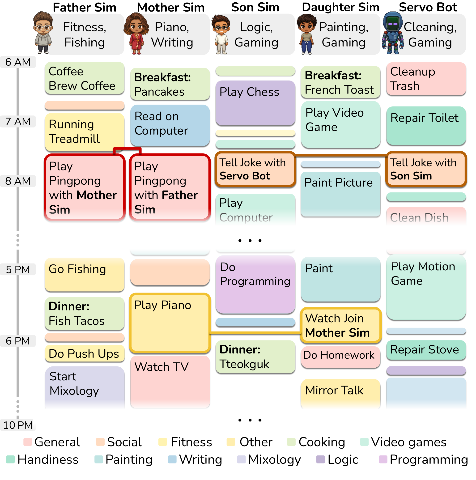
To evaluate this form of long-context understanding under controlled yet realistic conditions, we need simulation environments that support extended timelines and rich everyday behaviors. Existing embodied simulation platforms provide valuable testbeds for embodied tasks (Puig et al., 2018; Ren et al., 2026; Zhou et al., 2026; Puig et al., 2024), but long-term household routines with diverse contextual cues remain difficult to simulate at scale. To address this gap, we propose SimLife, a scalable platform for simulating long-term everyday life in a home-like environment. Built on The Sims 4²² 2 https://www.ea.com/games/the-sims/the-sims-4 This research is not endorsed by or affiliated with Electronic Arts (EA) or its licensors., SimLife supports scripted simulations of multi-character household activities with rich visual observations, synthetic dialogues with audio, vivid animations, and diverse event categories (Figure 2). We use this platform as a controllable foundation for constructing long-context benchmarks grounded in everyday behavior.

Refer to caption — Figure 1: SimLife-BP distribution overview. Left: action taxonomy with log-scaled counts. Right-top: episode lengths distribution, where one in-game day corresponds to 24 real minutes, or 0.4 real hours. Right-bottom: composition over three dimensions.

In this paper, we instantiate SimLife as SimLife-BP, a benchmark for behavioral pattern (BP) understanding: the ability to infer behavioral regularities, the rules behind them, and the temporal shifts that reshape them. SimLife-BP comprises 106 episodes averaging 15.49 hours and 38.57 in-game days, with up to 48.23 hours and 120 days per episode, and 1,439 questions in total. Each episode simulates a latent behavioral pattern governed by one or more rules and is accompanied by ground-truth action logs and topic-centered synthetic dialogues with audio for contextual grounding. To evaluate pattern understanding systematically, SimLife-BP combines two design axes: four question types that test direct, counterfactual, noisy, and inverse reasoning over inferred patterns, and three hint levels that vary how much rule information is provided, from explicit relevant conditions to abstract condition types to no prior hints. This design allows us to test whether models merely recognize surface regularities, or can robustly apply an inferred pattern across changing, distracting, and underspecified contexts.

Our evaluation reveals three main findings. Models can achieve high question-level accuracy without complete rule understanding, as they often answer forward predictions correctly but fail to transfer the rule to reverse reasoning. Second, models often reduce pattern inference to simple heuristics, such as frequency counting, instead of performing the necessary if-then reasoning. Finally, models struggle to update their understanding when the underlying pattern changes. Together, these findings show that long-context pattern understanding remains far from solved. More broadly, beyond the benchmark, SimLife opens up a wider space of long-horizon human-AI interaction challenges, providing a step toward embodied agents that can remember, adapt, and plan over extended periods of everyday life.

2 Related Work

Long Context Learning

Long-context learning has long been studied across application domains, from early work on document summarization and long-document understanding (Luhn, 1958; Edmundson, 1969; Salton et al., 1994) to modern long-context understanding (Beltagy et al., 2020; Liu et al., 2024; Kamradt, 2023; Jelassi et al., 2024), dialogue and chat history modeling (Bei et al., 2026), agentic tool use (Yao et al., 2023; Acharya et al., 2025; Fu et al., 2024), multimodal understanding (Long et al., 2026; Chen et al., 2026; Yan et al., 2025a), and embodied AI with persistent memory (Wang et al., 2024; Dai et al., 2026). Architecturally, this progress has been supported by increasingly large context windows (Reid et al., 2024; Bai et al., 2025a; Peng et al., 2024; Team, 2025), test-time adaptation (Ma et al., 2026; Zhang et al., 2025), continual learning (Deng et al., 2025), and self-evolving agents (Gao et al., 2026). Everyday assistants naturally fall into this setting, yet the growing scale and complexity of long-context benchmarks raise a key question: what makes a task uniquely long-context, beyond simply requiring longer inputs? Echoing with Hsieh et al. (2024); Bai et al. (2024); Bai et al. (2025b), SimLife-BP addresses this question by targeting intrinsically long-horizon reasoning rather than local retrieval over chunked segments, requiring models to integrate and cross-reference evidence scattered across days, weeks, and modalities to infer latent behavioral patterns.

Long Video Understanding

Long video understanding benchmarks have expanded across duration and modality, covering hour-long QA (Wu et al., 2024), extreme-length comprehension (Wang et al., 2025a), and egocentric scenarios (Grauman et al., 2022; Mangalam et al., 2023; Yang et al., 2025; Long et al., 2026; Chen et al., 2026; Yan et al., 2025a). Yet many still operationalize long-video understanding as retrieval or localization. SimLife-BP instead targets intrinsically cross-temporal understanding, where answers require integrating implicit evidence across multiple days, modalities, and interactions. By combining continuous daily-life simulations with controlled scripts and sampled agent profiles, SimLife-BP enables scalable, controllable evaluation of latent behavioral pattern inference.

Pattern Recognition

Pattern recognition spans perceptual regularity detection, sequential pattern mining, and abstract rule discovery (Bongard, 1970; Klahr and Dunbar, 1988; Josephson and Josephson, 1996; Agrawal and Srikant, 1995; Srikant and Agrawal, 1996; Mannila et al., 1997; Pei et al., 2001). Recent LLM benchmarks test rule induction from compact visual puzzles, symbolic examples, noisy observations, or programmatic input-output pairs (Chollet, 2019; Chollet et al., 2025; Hua et al., 2025; Li et al., 2025a; Li et al., 2025b). Long-context variants (Yan et al., 2025b; Kuratov et al., 2024) require aggregating many examples or scattered facts, but still use structured textual inputs. In contrast, SimLife-BP evaluates behavioral pattern recognition from unstructured ultra-long multimodal observations, requiring models to infer reusable latent rules from sparse, perceptually grounded, temporally distributed evidence.

3 SimLife Benchmark

3.1 Platform & Dataset

SimLife is built on The Sims 4, where we simulate multi-character household activities observed from the egocentric perspective of a serving robot called Servo Bot. Each simulated day spans 6 AM to 10 PM in-game, corresponding to approximately 24 minutes in real time. Figure 2 illustrates one example simulated day. Characters (or Sims) are initialized with a behavioral profile specifying probabilistic activity preferences, which shape their daily routines. We then sample 466 in-game days as dataset building blocks.

Each recorded simulated day is further enriched with synchronized ground-truth game logs filtered to Servo Bot’s field of view, spatialized conversational audio using Sim-specific voices, and context-generated dialogues. These dialogues range from natural everyday conversations to utterances that reference off-screen events or evolving situations.

3.2 Benchmark Design

Pattern Definition

We evaluate whether an agent can infer a simulated character’s behavioral pattern from ultra-long observations. Each pattern describes when a character performs or does not perform a target activity, based on temporal or event-based conditions. For example, a pattern “Bob drinks coffee on weekdays or after staying up late” links the activity of drinking coffee to both the day of the week and a prior-night event. To build an episode that reflects such a pattern, we filter and link simulated days together to build up a video chain that exhibits the target pattern over an extended period. The resulting sequence provides repeated, distributed evidence from which the model must infer the underlying rule to figure out the pattern. Details are provided in Appendix C.

Task Design

We evaluate models using grouped question answering in a streaming setting. After exposing the model to a sufficiently long video history, we pause the video and ask four binary multiple-choice questions that probe complementary forms of pattern understanding:

1.

Direct Prediction: Predict the most likely behavior given the current conditions.
2.

Counterfactual Prediction: Predict the most likely behavior under a hypothetical change in conditions.
3.

Noisy Counterfactual Prediction: Predict the most likely behavior under hypothetical conditions that include irrelevant information.
4.

Inverse Counterfactual Reasoning: Infer the most plausible condition or cause given an observed behavior.

Each behavioral pattern yields multiple tasks, inserted at query points chosen to cover different combinations of the pattern conditions. In the coffee example, we query the model on days corresponding to different combinations of weekday/weekend and with/without stayed-up-late. This allows us to test whether the model has learned the complete rule rather than a partial heuristic.

In addition, we evaluate each task under three hint levels that vary how much rule information is provided. In Full Hints, the relevant conditions are directly specified, e.g., “the activity is related to whether it is a weekday”. In Partial Hints, only the abstract type of each condition is revealed, e.g., “the activity is related to the day of the week”; this yields a closed hypothesis space while still requiring models to eliminate inconsistent rules from evidence. In No Hints, the model must infer the pattern entirely from observation (see Appendix D for more details).

Finally, to avoid asking questions before sufficient evidence is available, we use the Partial Hints setting as a reference point for query timing. Specifically, we run a hypothesis-elimination procedure over the observations and insert tasks only after the remaining hypotheses make predictions consistent with the ground-truth rule at the selected query point. This ensures that each task is, in principle, answerable from the accumulated evidence. More details are provided in Appendix E.

Benchmark Composition

As is shown in Figure 2, SimLife-BP contains 86 episodes for pattern understanding and 20 episodes for dynamic understanding. Pattern understanding episodes involve a single behavioral pattern, while dynamic understanding episodes involve multiple behavioral patterns and require models to identify distinct patterns as well as detect pattern shifts over time. Among them, 29 are solvable from vision alone, while 77 additionally require dialogue (audio).

To further probe contextual reasoning, 30% of episodes follow counterintuitive patterns, which associate activities with unusual or implausible conditions that cannot be inferred through common sense alone. For example, the pattern “drink coffee after playing the piano” is unlikely to arise from prior knowledge. Models must therefore rely primarily on evidence from the video context rather than world priors when answering questions.

4 Experiments

We evaluate AI models on pattern understanding in ultra-long contexts. Our study addresses three core research questions:

•

RQ1: Can AI models infer patterns from ultra-long-term observations? We assess the overall capability of models to recognize and reason about behavioral patterns accumulated over extended observation periods.
•

RQ2: How do AI models develop pattern understanding over time? We probe the models to explore how they incrementally build, refine, and revise their internal hypotheses across successive observations.
•

RQ3: How do AI models adapt to evolving patterns? We examine whether models can detect pattern changes, adapt their understanding accordingly, and retain knowledge of prior patterns without forgetting.

4.1 Experimental Setup

We design a series of experiments to investigate specific aspects of pattern understanding.

4.1.1 Pattern Understanding Overall (RQ1)

We designed experiments varying both the input modality and the degree of provided context. We evaluate models under four input conditions:

•

Vision + Language (V+L): Video frames (without audio) and dialogue transcripts.
•

Vision + Audio (V+A): Raw audio recordings of dialogue instead of transcript as part of the input.
•

Language Only (L): Event logs (action & dialogue) concatenated into a single input. This bypasses the vision process and uses ground-truth activities instead.
•

Language Only, noiseless (L-N): A filtered logs with main and directly related events.

Model Choice

We evaluate a broad set of models, including the Qwen3-VL family (4B, 8B, and 32B) (Bai et al., 2025a) with Chain-of-Thought (CoT) prompting; reasoning models with hybrid attention such as the Qwen3.5 (Qwen Team, 2026) and Gemma4 (Google, 2026) families, covering both dense and mixture-of-experts (MoE) variants; Qwen3-Omni (Xu et al., 2025) with an audio channel, and the Gemini (Google, 2025; Comanici et al., 2025) family as representative proprietary models. For vision-based input conditions, we follow the Socratic Models framework (Zeng et al., 2023): we divide each day’s video into four clips of approximately six minutes each, generate a summary for each clip, and concatenate all summaries with the task questions. For language-only variants, we concatenate the logs and questions into a single input pass. Implementation details are provided in Appendices J and K.

We also include representative agentic baselines designed for temporal search, i.e. VideoTree (Wang et al., 2025b), and memory management, i.e. M3-Agent (Long et al., 2026).

Hint Levels

We evaluate models with three hint levels as introduced in Section 3.2.

4.1.2 Trajectory Probing (RQ2)

We evaluate four representative models (Gemini-2.5-flash, Gemini-3-flash-preview, Gemma-4-26B-A4B-it, and Qwen3.5-35B-A3B) under the Language Only, Partial Hints setting. For each day $d$ in an episode, the model predicts whether the target activity will occur, yielding a daily belief trajectory $P_{d}(\text{yes})$ .

Rather than evaluating only the final prediction, this day-by-day trajectory captures how a model’s belief shifts from uncertainty to confidence as evidence accumulates. Since a model’s internal decision process is not directly observable, we compare its trajectory against interpretable reference baselines as behavioral probes: if a model’s predictions closely track a baseline, this suggests that it may be following a similar decision strategy.

We consider five reference baselines. Two are shallow heuristics that do not perform rule inference: (B1) frequency-based, predicting from the historical base rate, and (B2) last-day-based, extrapolating from the previous day’s outcome. Three are advanced references: (B3) ground-truth oracle, (B4) human predictions (Appendix H), and (B5) hypothesis-elimination, which prunes candidate rules against accumulated evidence (Appendix E).

4.1.3 Pattern Adaptation (RQ3)

Patterns may evolve over time for arbitrary reasons. To evaluate models’ ability to adapt to evolving patterns, we design two experimental conditions.

First, we examine whether models can rapidly adapt to pattern changes when the change is implicitly signaled through dialogue, such as when a character mentions that summer vacation has started, or the schedule gets tighter. This setting is part of our benchmark design, as described in Section 3.2.

Second, after a model observes a sequence governed first by Pattern 1 and then by Pattern 2, we query it about events from the Pattern 1 period to assess whether prior knowledge is retained or overwritten.

Model	FPS	Thinking	Full Hints			Partial Hints			No Hints
Model	FPS	Thinking	AC	Acc	Sub Acc	AC	Acc	Sub Acc	AC	Acc	Sub Acc
Vision + Language (V+L)
Qwen3-VL-4B-Instruct	0.5	CoT	$10.5^{\,\scalebox{0.7}{$\pm 3.1$}}$	$50.2^{\,\scalebox{0.7}{$\pm 2.6$}}$		$11.8^{\,\scalebox{0.7}{$\pm 3.2$}}$	$50.6^{\,\scalebox{0.7}{$\pm 2.6$}}$		$8.9^{\,\scalebox{0.7}{$\pm 2.9$}}$	$50.9^{\,\scalebox{0.7}{$\pm 2.6$}}$
Qwen3-VL-8B-Instruct	0.5	CoT	$8.9^{\,\scalebox{0.7}{$\pm 2.9$}}$	$49.1^{\,\scalebox{0.7}{$\pm 2.6$}}$		$11.0^{\,\scalebox{0.7}{$\pm 3.1$}}$	$50.6^{\,\scalebox{0.7}{$\pm 2.6$}}$		$7.1^{\,\scalebox{0.7}{$\pm 2.6$}}$	$49.3^{\,\scalebox{0.7}{$\pm 2.6$}}$
Qwen3-VL-32B-Instruct	0.5	CoT	$11.0^{\,\scalebox{0.7}{$\pm 3.1$}}$	$51.9^{\,\scalebox{0.7}{$\pm 2.6$}}$		$13.6^{\,\scalebox{0.7}{$\pm 3.4$}}$	$53.2^{\,\scalebox{0.7}{$\pm 2.6$}}$		$12.1^{\,\scalebox{0.7}{$\pm 3.3$}}$	$53.0^{\,\scalebox{0.7}{$\pm 2.6$}}$
Qwen3.5-9B	0.5	R	$12.3^{\,\scalebox{0.7}{$\pm 3.3$}}$	$48.9^{\,\scalebox{0.7}{$\pm 2.6$}}$		$14.2^{\,\scalebox{0.7}{$\pm 3.5$}}$	$51.4^{\,\scalebox{0.7}{$\pm 2.6$}}$		$13.4^{\,\scalebox{0.7}{$\pm 3.4$}}$	$51.0^{\,\scalebox{0.7}{$\pm 2.6$}}$
Qwen3.5-35B-A3B	0.5	R	$13.1^{\,\scalebox{0.7}{$\pm 3.4$}}$	$52.2^{\,\scalebox{0.7}{$\pm 2.6$}}$		$14.2^{\,\scalebox{0.7}{$\pm 3.5$}}$	$53.3^{\,\scalebox{0.7}{$\pm 2.6$}}$		$12.3^{\,\scalebox{0.7}{$\pm 3.3$}}$	$52.5^{\,\scalebox{0.7}{$\pm 2.6$}}$
Gemma-4-26B-A4B-it	0.5	R	$7.6^{\,\scalebox{0.7}{$\pm 2.7$}}$	$48.8^{\,\scalebox{0.7}{$\pm 2.6$}}$		$7.6^{\,\scalebox{0.7}{$\pm 2.7$}}$	$48.1^{\,\scalebox{0.7}{$\pm 2.6$}}$		$10.8^{\,\scalebox{0.7}{$\pm 3.1$}}$	$49.3^{\,\scalebox{0.7}{$\pm 2.6$}}$
Gemini-3-flash-preview	0.5	R	$14.7^{\,\scalebox{0.7}{$\pm 3.6$}}$	$53.0^{\,\scalebox{0.7}{$\pm 2.6$}}$		$13.9^{\,\scalebox{0.7}{$\pm 3.5$}}$	$54.1^{\,\scalebox{0.7}{$\pm 2.6$}}$		$14.2^{\,\scalebox{0.7}{$\pm 3.5$}}$	$54.8^{\,\scalebox{0.7}{$\pm 2.6$}}$
VideoTree (Mixtral-8x7B)	1	CoT	$11.0^{\,\scalebox{0.7}{$\pm 3.1$}}$	$54.0^{\,\scalebox{0.7}{$\pm 2.6$}}$		$9.7^{\,\scalebox{0.7}{$\pm 3.0$}}$	$51.7^{\,\scalebox{0.7}{$\pm 2.6$}}$		$10.8^{\,\scalebox{0.7}{$\pm 3.1$}}$	$52.6^{\,\scalebox{0.7}{$\pm 2.6$}}$
Vision + Audio (V+A)
Qwen3-Omni-30B-A3B + Qwen3.5-9B	0.5	R	$10.8^{\,\scalebox{0.7}{$\pm 3.1$}}$	$48.1^{\,\scalebox{0.7}{$\pm 2.6$}}$		$11.0^{\,\scalebox{0.7}{$\pm 3.1$}}$	$48.6^{\,\scalebox{0.7}{$\pm 2.6$}}$		$10.8^{\,\scalebox{0.7}{$\pm 3.1$}}$	$48.6^{\,\scalebox{0.7}{$\pm 2.6$}}$
M3-Agent	1	R	$10.0^{\,\scalebox{0.7}{$\pm 3.0$}}$	$53.4^{\,\scalebox{0.7}{$\pm 2.6$}}$		$10.2^{\,\scalebox{0.7}{$\pm 3.0$}}$	$55.0^{\,\scalebox{0.7}{$\pm 2.6$}}$		$12.1^{\,\scalebox{0.7}{$\pm 3.3$}}$	$54.6^{\,\scalebox{0.7}{$\pm 2.6$}}$
Language Only (L)
Qwen3.5-9B	–	R	$9.2^{\,\scalebox{0.7}{$\pm 2.9$}}$	$50.9^{\,\scalebox{0.7}{$\pm 2.6$}}$		$13.6^{\,\scalebox{0.7}{$\pm 3.4$}}$	$54.6^{\,\scalebox{0.7}{$\pm 2.6$}}$		$14.2^{\,\scalebox{0.7}{$\pm 3.5$}}$	$54.6^{\,\scalebox{0.7}{$\pm 2.6$}}$
Qwen3.5-35B-A3B	–	R	$18.1^{\,\scalebox{0.7}{$\pm 3.9$}}$	$61.1^{\,\scalebox{0.7}{$\pm 2.5$}}$		$18.4^{\,\scalebox{0.7}{$\pm 3.9$}}$	$59.3^{\,\scalebox{0.7}{$\pm 2.5$}}$		$16.0^{\,\scalebox{0.7}{$\pm 3.7$}}$	$58.7^{\,\scalebox{0.7}{$\pm 2.5$}}$
Gemma-4-26B-A4B-it	–	R	$11.3^{\,\scalebox{0.7}{$\pm 3.2$}}$	$53.9^{\,\scalebox{0.7}{$\pm 2.6$}}$		$11.0^{\,\scalebox{0.7}{$\pm 3.1$}}$	$54.4^{\,\scalebox{0.7}{$\pm 2.6$}}$		$11.3^{\,\scalebox{0.7}{$\pm 3.2$}}$	$54.8^{\,\scalebox{0.7}{$\pm 2.6$}}$
Gemini-2.5-flash	–	R	$17.9^{\,\scalebox{0.7}{$\pm 3.8$}}$	$58.6^{\,\scalebox{0.7}{$\pm 2.6$}}$		$21.0^{\,\scalebox{0.7}{$\pm 4.1$}}$	$60.2^{\,\scalebox{0.7}{$\pm 2.5$}}$		$16.3^{\,\scalebox{0.7}{$\pm 3.7$}}$	$56.4^{\,\scalebox{0.7}{$\pm 2.6$}}$
Gemini-3-flash-preview	–	R	$27.8^{\,\scalebox{0.7}{$\pm 4.5$}}$	$69.2^{\,\scalebox{0.7}{$\pm 2.4$}}$		$\textbf{\lx@text@underline{33.3}}^{\,\scalebox{0.7}{$\pm 4.7$}}$	$69.4^{\,\scalebox{0.7}{$\pm 2.4$}}$		$27.8^{\,\scalebox{0.7}{$\pm 4.5$}}$	$66.5^{\,\scalebox{0.7}{$\pm 2.4$}}$
Gemini-3.1-flash-lite	–	R	$20.7^{\,\scalebox{0.7}{$\pm 4.1$}}$	$59.9^{\,\scalebox{0.7}{$\pm 2.5$}}$		$21.0^{\,\scalebox{0.7}{$\pm 4.1$}}$	$61.2^{\,\scalebox{0.7}{$\pm 2.5$}}$		$18.6^{\,\scalebox{0.7}{$\pm 3.9$}}$	$59.1^{\,\scalebox{0.7}{$\pm 2.5$}}$
Language only, noiseless (L-N)
Qwen3.5-9B	–	R	$23.6^{\,\scalebox{0.7}{$\pm 4.3$}}$	$65.5^{\,\scalebox{0.7}{$\pm 2.5$}}$		$18.4^{\,\scalebox{0.7}{$\pm 3.9$}}$	$61.2^{\,\scalebox{0.7}{$\pm 2.5$}}$		$16.0^{\,\scalebox{0.7}{$\pm 3.7$}}$	$56.5^{\,\scalebox{0.7}{$\pm 2.6$}}$
Qwen3.5-35B-A3B	–	R	$34.9^{\,\scalebox{0.7}{$\pm 4.8$}}$	$73.0^{\,\scalebox{0.7}{$\pm 2.3$}}$		$32.0^{\,\scalebox{0.7}{$\pm 4.7$}}$	$\textbf{\lx@text@underline{70.3}}^{\,\scalebox{0.7}{$\pm 2.4$}}$		$21.5^{\,\scalebox{0.7}{$\pm 4.1$}}$	$62.7^{\,\scalebox{0.7}{$\pm 2.5$}}$
Gemma-4-26B-A4B-it	–	R	$30.2^{\,\scalebox{0.7}{$\pm 4.6$}}$	$72.1^{\,\scalebox{0.7}{$\pm 2.3$}}$		$26.0^{\,\scalebox{0.7}{$\pm 4.4$}}$	$68.4^{\,\scalebox{0.7}{$\pm 2.4$}}$		$22.3^{\,\scalebox{0.7}{$\pm 4.2$}}$	$64.1^{\,\scalebox{0.7}{$\pm 2.5$}}$
Gemma-4-31B-it	–	R	$\textbf{\lx@text@underline{36.2}}^{\,\scalebox{0.7}{$\pm 4.8$}}$	$\textbf{\lx@text@underline{74.6}}^{\,\scalebox{0.7}{$\pm 2.2$}}$		$30.2^{\,\scalebox{0.7}{$\pm 4.6$}}$	$69.6^{\,\scalebox{0.7}{$\pm 2.4$}}$		$\textbf{\lx@text@underline{29.4}}^{\,\scalebox{0.7}{$\pm 4.6$}}$	$\textbf{\lx@text@underline{67.6}}^{\,\scalebox{0.7}{$\pm 2.4$}}$
Gemini-2.5-flash	–	R	$31.5^{\,\scalebox{0.7}{$\pm 4.7$}}$	$71.8^{\,\scalebox{0.7}{$\pm 2.3$}}$		$22.3^{\,\scalebox{0.7}{$\pm 4.2$}}$	$65.3^{\,\scalebox{0.7}{$\pm 2.5$}}$		$22.1^{\,\scalebox{0.7}{$\pm 4.2$}}$	$63.7^{\,\scalebox{0.7}{$\pm 2.5$}}$
Gemini-3-flash-preview	–	R	$24.1^{\,\scalebox{0.7}{$\pm 4.3$}}$	$68.2^{\,\scalebox{0.7}{$\pm 2.4$}}$		$24.9^{\,\scalebox{0.7}{$\pm 4.3$}}$	$67.3^{\,\scalebox{0.7}{$\pm 2.4$}}$		$23.1^{\,\scalebox{0.7}{$\pm 4.2$}}$	$63.9^{\,\scalebox{0.7}{$\pm 2.5$}}$

Table 1: Main results on SimLife-BP (381 tasks / 1,439 questions per hint level). We report All-Correct rate (AC) and question-level accuracy (Acc) with 95% binomial CI half-widths. Each Sub Acc cell shows per-question-type accuracy, left-to-right: Direct, Counterfactual, Noise Counterfactual, Inverse Counterfactual; the gray line marks chance. Shading highlights within-row best variants, and bold marks the overall best in each column.

4.2 Evaluation Metrics

For RQ1 and RQ3, we report two primary metrics: All-Correct Rate (AC), the proportion of tasks for which the model answers all sub-questions correctly, reflecting the consistency and completeness of its pattern understanding; Average Accuracy Rate (Acc), the mean accuracy across all sub-questions within a task, as well as Sub-questions Accuracy (Sub Acc), providing a finer-grained performance measure.

For RQ2, we analyze the models’ daily predicted probabilities for yes/no answers. We use the Brier score (Brier, 1950) to measure the discrepancy between predicted probabilities and ground-truth outcomes. Accuracy (Acc), balanced accuracy (B-Acc), positive F1-score (F1⁺), and averaged $P(\text{yes})$ ( $\bar{p}_{\mathrm{yes}}$ ) are also reported for reference. In addition, we report Spearman correlation between each model’s daily prediction trajectory and the five reference baselines described above.

5 Results & Discussion

Figure 4: Per-day trajectories of model predictions and human judgments. A rapid convergence of Brier score (bottom) toward zero after hypothesis elimination indicates successful pattern understanding and retention.

Source	[1]	[2]	[3]	[4]	[5]	[6]	[7]	[8]	[9]	$n$	Acc	B-Acc	F1⁺	Brier $\downarrow$	$\bar{p}_{\mathrm{yes}}$
Language Only (L)
[1] Qwen3.5-35B-A3B	100.0	22.0	20.4	21.4	15.2	28.8	26.2	19.6	23.7	4067	59.7	61.3	46.1	39.8	48.1
[2] Gemma-4-26B-A4B-it	22.0	100.0	18.8	31.4	22.0	32.2	12.8	23.6	25.0	4017	64.0	64.0	48.7	36.0	43.5
[3] Gemini-2.5-flash	20.4	18.8	100.0	21.4	21.7	38.5	22.1	21.4	29.2	4068	71.6	59.6	39.0	28.4	20.1
[4] Gemini-3-flash-preview	21.4	31.4	21.4	100.0		30.4	9.6	38.8	40.5	4053	74.0	70.7	56.5	26.0	33.4
Human Study
[5] Human-prediction	15.2	22.0	21.7	46.7	100.0	17.6	4.8	74.3	78.1	194 $\times$ 3	84.5	83.3	79.2	9.8	39.4
Reference Baselines
[6] Frequency-based	28.8	32.2	38.5	30.4	17.6	100.0	52.0	37.0	50.2	4068	73.0	63.3	45.6	17.0	29.2
[7] Last-day-based	26.2	12.8	22.1	9.6	4.8	52.0	100.0	12.7	19.3	4068	65.3	56.5	36.7	33.7	26.9
[8] Ground-truth-based	19.6	23.6	21.4	38.8	74.3	37.0	12.7	100.0	79.2	4068	100.0	100.0	100.0	0.0	26.6
[9] Hypothesis-elimination-based	23.7	25.0	29.2	40.5	78.1	50.2	19.3	79.2	100.0	4068	88.7	88.0	80.2	6.5	27.7

Table 2: Spearman rank correlation of

P_{d}(\text{yes})

trajectories (%). Blue/light blue: best/second-best non-self correlation per row ([1]–[5]). Orange/light orange: best/second-best per column ([5], Acc, B-Acc, F1⁺, Brier).

5.1 Pattern Understanding Overall (RQ1)

Table 1 shows that performance improves substantially as inputs become cleaner and more structured. In the V+L setting, most models remain near chance on Acc, with only Gemini 3 Flash exceeding chance across hint levels. In contrast, models consistently perform above chance in the L-N setting, with Gemma-4-31B-it reaching $36.2\%$ AC and $74.6\%$ Acc with Full Hints. However, even this best oracle-filtered result remains far from solved, suggesting a bottleneck caused by both long multimodal evidence extraction and latent rule inference.

V+L models perform best under Partial Hints, L shows mixed behavior, and Full Hints shows the best performance for L-N. This pattern suggests that precise condition hints are useful only when models can ground the corresponding evidence. When perceptual or summary signals are noisy, specifying the relevant variables alone does not guarantee better rule application.

Forward-only Shortcutting.

The per-question-type breakdown (Sub Acc) reveals a consistent asymmetry: forward counterfactual questions (CF) are much easier than inverse (IC) and noise-injected (NC) variants, and this gap widens as inputs become cleaner: under No Hints, the median CF-IC gap increases from +4.2% in V+L to +16.2% in L and +32.1% in L-N, while IC accuracy changes little. The task-level AC reflects the same pattern: Gemma-4-31B-it (L-N) reaches 86.6% on CF alone but only 36.2% AC. Together, these results indicate that models latch onto forward-specific patterns rather than inferring the underlying rule, since genuine rule understanding would yield near-symmetric performance across question types.

5.2 Trajectory Probing (RQ2)

Table 2 reports the pairwise Spearman correlations among the $P_{d}(\text{yes})$ trajectories across all sources, measuring how similarly each trajectory evolves over the chain. For Qwen, Gemma, and Gemini 2.5 Flash, the strongest non-self correlation is with the frequency-based baseline (28.8%, 32.2%, 38.5% respectively). These results suggest that, given partial hints, models tend to default to simple heuristics, like counting instances of the target activity, rather than evaluating candidate rules against the accumulated evidence.

The exception is Gemini 3 Flash, whose closest non-self reference baseline is hypothesis elimination (40.5%), and is also the most aligned with human predictions (46.7%). By construction, the hypothesis-elimination baseline captures the sequential process of pruning candidate rules against observed evidence. Human predictions are strongly correlated with this baseline (78.1%), indicating that humans follow this rule-pruning process and do so effectively. These results suggest that Gemini 3 Flash exhibits a certain degree of hypothesis elimination and produces more human-like uncertainty trajectories over the chain. In contrast, the other models appear more strongly anchored by frequency and recency heuristics, showing weaker evidence of systematic hypothesis elimination.

Representative Examples.

Figure 4 unpacks the aggregate correlations on two chains selected from the human study (see Appendix H). The first case N0 (“Mother paints every Tuesday”) is the easiest pattern that hypothesis-elimination resolves within the first week (green area). Both Gemini 3 Flash and Gemma stay close to the human curve here, while Gemini 2.5 Flash picks up the signal early on but reverts to “no” for the end of the chain. The second case, N7 (“Daughter plays games every Mon/Tue/Wed/Thu, but then plays only on weekends after she gets busy”), contains a pattern shift at day 14. Humans and Gemini 3 Flash adapt quickly: Brier scores on post-pivot weekdays initially spike due to the old pattern, but they return to near zero within a week. In contrast, Gemini 2.5 Flash, Gemma, and Qwen remain locked onto the original rule and continue predicting “yes” on weekdays for the rest of the chain.³³ 3 We note one fairness asymmetry: humans receive an explicit notice (“the behavior pattern may change after this point”), whereas models must infer the shift through dialogue, thus the post-pivot gap reflects both the scaffolding difference and a failure to recognize that dialogue indicates a change.

Three observations explain the alignment between aggregate ranking and the per-case shapes. First, Gemma and Qwen are heavily overconfident, placing 97–100% of predictions at $P(\text{yes}){\leq}0.05$ or ${\geq}0.95$ , compared to 37% for humans, so each mistake incurs the full Brier penalty rather than the smaller cost of a hedged prediction. Second, on static conditional chains (N1–N3 in Appendix I), no model consistently executes the required if-then reasoning, instead substituting cheaper heuristics, such as keyword matching, producing trajectories more like the frequency-based reference baseline rather than hypothesis elimination. Third, on dynamic chains, regime-change dialogue appears in all post-pivot contexts but is referenced in only 1–12% of the post-pivot reasoning traces. Correspondingly, post-pivot Brier rises by $+0.09$ to $+0.14$ across the open models, showing they continue using the first pattern’s rule rather than resetting the hypothesis space.

Overall, Gemini 3 Flash is the one model whose reasoning traces consistently show explicit cycle detection and post-pivot dialogue use, matching its stronger correlation with both hypothesis-elimination baseline and human prediction.

5.3 Pattern Adaptation (RQ3)

	Model	P1	P2	Hist	P1-P2	Hist-P1	Hist-P2
L	Qwen3.5-35B-A3B	63.4	48.7	65.3	+14.8^∗	+1.8	+16.6^∗
L	Gemini-3-flash	86.9	61.3	74.5	+25.6^∗∗∗	-12.4^∗∗	+13.2^∗
L-N	Qwen3.5-35B-A3B	85.5	65.3	77.3	+20.2^∗∗∗	-8.2^∗∗	+12.0
L-N	Gemini-3-flash	79.3	65.3	76.4	+14.0^∗	-2.9	+11.1
V/Agent	Gemini-3-flash (V+L)	57.9	56.7	55.6	+1.3	-2.4	-1.1
	VideoTree (retrieval)	48.3	51.3	59.3	-3.1	+11.0	+7.9
	M3-Agent (memory)	60.7	56.7	57.9	+4.0	-2.8	+1.2

Table 3: Pattern adaptation of representative baselines (partial-hint, question-level accuracy in %). Stars indicate task-level Mann-Whitney significance (

{}^{*}p\!<\!.05

{}^{**}p\!<\!.01

{}^{***}p\!<\!.001

). See full results in Table 20.

We evaluate dynamic understanding across 20 episodes, each consisting of two sequential behavioral patterns, using three task types: P1, questions about Pattern 1 while active; P2, questions about Pattern 2 after pattern shift and sufficient exposure to the new pattern; and Hist, questions about the earlier Pattern 1 after observing Pattern 2. Representative results appear in Table 3.

Under L and L-N settings, the order of performance is consistently P1, then Hist, then P2. The P1 $\rightarrow$ P2 gap is significant for every model, reaching +25.6 $\%$ ( $p\!<\!.001$ ) for Gemini 3 Flash, showing that models can identify a schedule, but struggle to update once it changes. The limitation is therefore online integration of the new pattern rather than recall of the past. This gap shrinks but does not close for stronger models (see Table 20).

Hist Retrieval Shortcut.

Notably, we expected Hist to be the hardest setting with the worst performance, because it requires retaining the earlier pattern while resisting interference from the current one; yet models generally perform better on Hist than P2. We attribute this to a shortcut our design intended to avoid but that persists in full-context models: because pre-switch evidence remains verbatim in the context, models can answer Hist through local pattern-matching rather than by reasoning about the pattern transition. Accuracy is consistent with this reading: Hist sits far above P2, yet stays below the clean P1 (-12.4%, $p\!<\!.01$ for Gemini 3 Flash, L) condition, likely because post-shift content dilutes but does not prevent retrieval. Temporal anchors were intentionally vague (e.g., “roughly one month ago”) to discourage this shortcut, but wording had no effect on accuracy.

6 Conclusion & Future Work

We presented SimLife, a platform for simulating long-term everyday life, and SimLife-BP, a benchmark for evaluating pattern understanding from ultra-long multimodal observations. Our results show that current models often rely on surface heuristics, fail to apply inferred rules robustly, and struggle to adapt to pattern shifts. These findings highlight long-context pattern understanding as an open challenge for embodied AI, and SimLife provides a foundation for studying memory, personalization, adaptation, and long-horizon planning in everyday human-AI interaction.

Acknowledgments

We gratefully acknowledge the Google Cloud Research Credits Program for providing credits that supported the Gemini API usage in this work. We also thank Yutong Wang for valuable assistance during the preliminary exploration of this project.

References

Acharya et al. (2025) D. B. Acharya, K. Kuppan, and B. Divya Agentic ai: autonomous intelligence for complex goals—a comprehensive survey. IEEE Access 13, pp. 18912–18936. External Links: Document Cited by: §2.
Agrawal and Srikant (1995) R. Agrawal and R. Srikant Mining sequential patterns. In Proceedings of the Eleventh International Conference on Data Engineering, ICDE ’95, USA, pp. 3–14. External Links: ISBN 0818669101 Cited by: §2.
Bai et al. (2025a) S. Bai, Y. Cai, R. Chen, K. Chen, X. Chen, Z. Cheng, L. Deng, W. Ding, C. Gao, C. Ge, et al. Qwen3-vl technical report. arXiv preprint arXiv:2511.21631. Cited by: §2, §4.1.1.
Bai et al. (2024) Y. Bai, X. Lv, J. Zhang, H. Lyu, J. Tang, Z. Huang, Z. Du, X. Liu, A. Zeng, L. Hou, Y. Dong, J. Tang, and J. Li LongBench: a bilingual, multitask benchmark for long context understanding. In Proceedings of the 62nd Annual Meeting of the Association for Computational Linguistics (Volume 1: Long Papers), pp. 3119–3137. External Links: Link, Document Cited by: §2.
Bai et al. (2025b) Y. Bai, S. Tu, J. Zhang, H. Peng, X. Wang, X. Lv, S. Cao, J. Xu, L. Hou, Y. Dong, J. Tang, and J. Li LongBench v2: towards deeper understanding and reasoning on realistic long-context multitasks. In Proceedings of the 63rd Annual Meeting of the Association for Computational Linguistics (Volume 1: Long Papers), pp. 3639–3664. External Links: Link, Document, ISBN 979-8-89176-251-0 Cited by: §2.
Bei et al. (2026) Y. Bei, T. Wei, X. Ning, Y. Zhao, Z. Liu, X. Lin, Y. Zhu, H. Hamann, J. He, and H. Tong Mem-gallery: benchmarking multimodal long-term conversational memory for mllm agents. arXiv preprint arXiv:2601.03515. Cited by: §2.
Beltagy et al. (2020) I. Beltagy, M. E. Peters, and A. Cohan Longformer: the long-document transformer. arXiv:2004.05150. Cited by: §2.
Bongard (1970) M. M. Bongard Pattern recognition. Spartan Books, New York. Note: Translated from Russian External Links: Link Cited by: §2.
Brier (1950) G. W. Brier VERIFICATION of forecasts expressed in terms of probability. Monthly Weather Review 78 (1), pp. 1 – 3. External Links: Document, Link Cited by: §4.2.
Chen et al. (2026) G. Chen, L. Lu, Y. Liu, L. Dong, L. Zou, J. Lv, Z. Li, X. Mao, B. Pei, S. Wang, Z. Li, K. Sapra, F. Liu, Y. Zheng, Y. Huang, L. Wang, Z. Yu, A. Tao, G. Liu, and T. Lu Towards multimodal lifelong understanding: a dataset and agentic baseline. External Links: 2603.05484, Link Cited by: §2, §2.
Chollet et al. (2025) F. Chollet, M. Knoop, G. Kamradt, B. Landers, and H. Pinkard Arc-agi-2: a new challenge for frontier ai reasoning systems. arXiv preprint arXiv:2505.11831. Cited by: §2.
Chollet (2019) F. Chollet On the measure of intelligence. arXiv preprint arXiv:1911.01547. Cited by: §2.
Comanici et al. (2025) G. Comanici, E. Bieber, M. Schaekermann, I. Pasupat, N. Sachdeva, I. Dhillon, M. Blistein, O. Ram, D. Zhang, E. Rosen, et al. Gemini 2.5: pushing the frontier with advanced reasoning, multimodality, long context, and next generation agentic capabilities. arXiv preprint arXiv:2507.06261. Cited by: §4.1.1.
Dai et al. (2026) Y. Dai, H. Fu, J. Lee, Y. Liu, H. Zhang, J. Yang, C. Finn, N. Fazeli, and J. Chai RoboMME: benchmarking and understanding memory for robotic generalist policies. arXiv preprint arXiv:2603.04639. Cited by: §2.
Deng et al. (2025) J. Deng, Q. Wu, P. Ju, S. Lin, Y. Liang, and N. Shroff Unlocking the power of rehearsal in continual learning: a theoretical perspective. In Forty-second International Conference on Machine Learning, External Links: Link Cited by: §2.
Edmundson (1969) H. P. Edmundson New methods in automatic extracting. J. ACM 16, pp. 264–285. External Links: Link Cited by: §2.
Fu et al. (2024) Y. Fu, D. Kim, J. Kim, S. Sohn, L. Logeswaran, K. Bae, and H. Lee AutoGuide: automated generation and selection of context-aware guidelines for large language model agents. In The Thirty-eighth Annual Conference on Neural Information Processing Systems, External Links: Link Cited by: §2.
Gao et al. (2026) H. Gao, J. Geng, W. Hua, M. Hu, X. Juan, H. Liu, S. Liu, J. Qiu, X. Qi, Q. Ren, Y. Wu, H. Wang, H. Xiao, Y. Zhou, S. Zhang, J. Zhang, J. Xiang, Y. Fang, Q. Zhao, D. Liu, C. Qian, Z. Wang, M. Hu, H. Wang, Q. Wu, H. Ji, and M. Wang A survey of self-evolving agents: what, when, how, and where to evolve on the path to artificial super intelligence. Transactions on Machine Learning Research. Note: Survey Certification External Links: ISSN 2835-8856, Link Cited by: §2.
Google (2025) Google Gemini 3 flash preview. Note: https://ai.google.dev/gemini-api/docs/models/gemini-3-flash-previewModel ID: gemini-3-flash-preview. Accessed: 2026-05-20 Cited by: §4.1.1.
Google (2026) Google Gemma 4 model card. Note: https://ai.google.dev/gemma/docs/core/model_card_4Accessed: 2026-05-20 Cited by: §4.1.1.
Grauman et al. (2022) K. Grauman, A. Westbury, E. Byrne, Z. Chavis, A. Furnari, R. Girdhar, J. Hamburger, H. Jiang, M. Liu, X. Liu, M. Martin, T. Nagarajan, I. Radosavovic, S. K. Ramakrishnan, F. Ryan, J. Sharma, M. Wray, M. Xu, E. Z. Xu, C. Zhao, S. Bansal, D. Batra, V. Cartillier, S. Crane, T. Do, M. Doulaty, A. Erapalli, C. Feichtenhofer, A. Fragomeni, Q. Fu, A. Gebreselasie, C. González, J. Hillis, X. Huang, Y. Huang, W. Jia, W. Khoo, J. Koláĭ, S. Kottur, A. Kumar, F. Landini, C. Li, Y. Li, Z. Li, K. Mangalam, R. Modhugu, J. Munro, T. Murrell, T. Nishiyasu, W. Price, P. R. Puentes, M. Ramazanova, L. Sari, K. Somasundaram, A. Southerland, Y. Sugano, R. Tao, M. Vo, Y. Wang, X. Wu, T. Yagi, Z. Zhao, Y. Zhu, P. Arbeláez, D. Crandall, D. Damen, G. M. Farinella, C. Fuegen, B. Ghanem, V. K. Ithapu, C. V. Jawahar, H. Joo, K. Kitani, H. Li, R. Newcombe, A. Oliva, H. S. Park, J. M. Rehg, Y. Sato, J. Shi, M. Z. Shou, A. Torralba, L. Torresani, M. Yan, and J. Malik Ego4D: around the world in 3,000 hours of egocentric video. In 2022 IEEE/CVF Conference on Computer Vision and Pattern Recognition (CVPR), pp. 18973–18990. External Links: Document Cited by: §2.
Hsieh et al. (2024) C. Hsieh, S. Sun, S. Kriman, S. Acharya, D. Rekesh, F. Jia, and B. Ginsburg RULER: what’s the real context size of your long-context language models?. In First Conference on Language Modeling, External Links: Link Cited by: §2.
Hua et al. (2025) W. Hua, T. Wong, F. Sun, L. Pan, A. Jardine, and W. Y. Wang InductionBench: LLMs fail in the simplest complexity class. In Proceedings of the 63rd Annual Meeting of the Association for Computational Linguistics (Volume 1: Long Papers), W. Che, J. Nabende, E. Shutova, and M. T. Pilehvar (Eds.), Vienna, Austria, pp. 26526–26546. External Links: Link, Document, ISBN 979-8-89176-251-0 Cited by: §2.
Jelassi et al. (2024) S. Jelassi, D. Brandfonbrener, S. M. Kakade, and E. Malach Repeat after me: transformers are better than state space models at copying. In Proceedings of the 41st International Conference on Machine Learning, R. Salakhutdinov, Z. Kolter, K. Heller, A. Weller, N. Oliver, J. Scarlett, and F. Berkenkamp (Eds.), Proceedings of Machine Learning Research, Vol. 235, pp. 21502–21521. External Links: Link Cited by: §2.
Josephson and Josephson (1996) J. R. Josephson and S. G. Josephson Abductive inference: computation, philosophy, technology. Cambridge University Press. Cited by: §2.
Kamradt (2023) G. Kamradt Needle In A Haystack: pressure testing llms. Note: https://github.com/gkamradt/LLMTest_NeedleInAHaystackGitHub repository. Accessed: 2026-05-25 Cited by: §2.
Klahr and Dunbar (1988) D. Klahr and K. Dunbar Dual space search during scientific reasoning. Cognitive science 12 (1), pp. 1–48. Cited by: §2.
Kuratov et al. (2024) Y. Kuratov, A. Bulatov, P. Anokhin, I. Rodkin, D. Sorokin, A. Sorokin, and M. Burtsev BABILong: testing the limits of LLMs with long context reasoning-in-a-haystack. arXiv preprint arXiv:2406.10149. Cited by: §2.
Li et al. (2025a) C. Li, W. Wang, T. Zheng, and Y. Song Patterns over principles: the fragility of inductive reasoning in LLMs under noisy observations. In Findings of the Association for Computational Linguistics: ACL 2025, W. Che, J. Nabende, E. Shutova, and M. T. Pilehvar (Eds.), Vienna, Austria, pp. 19608–19626. External Links: Link, Document, ISBN 979-8-89176-256-5 Cited by: §2.
Li et al. (2025b) J. Li, P. Cao, Z. Jin, Y. Chen, K. Liu, and J. Zhao MIRAGE: evaluating and explaining inductive reasoning process in language models. In The Thirteenth International Conference on Learning Representations, External Links: Link Cited by: §2.
Liu et al. (2024) N. F. Liu, K. Lin, J. Hewitt, A. Paranjape, M. Bevilacqua, F. Petroni, and P. Liang Lost in the middle: how language models use long contexts. Transactions of the Association for Computational Linguistics 12, pp. 157–173. External Links: Link, Document Cited by: §2.
Long et al. (2026) L. Long, Y. He, W. Ye, Y. Pan, Y. Lin, H. Li, J. Zhao, and W. Li Seeing, listening, remembering, and reasoning: a multimodal agent with long-term memory. In The Fourteenth International Conference on Learning Representations, External Links: Link Cited by: §J.5, §2, §2, §4.1.1.
Luhn (1958) H. P. Luhn The automatic creation of literature abstracts. IBM Journal of Research and Development 2 (2), pp. 159–165. External Links: Document Cited by: §2.
Ma et al. (2023) Z. Ma, J. Sansom, R. Peng, and J. Chai Towards a holistic landscape of situated theory of mind in large language models. Findings of Empirical Methods in Natural Language Processing. Cited by: §1.
Ma et al. (2026) Z. Ma, X. Yu, H. Zhen, Y. Yang, J. Chai, and C. Gan Fast spatial memory with elastic test-time training. arXiv preprint arXiv:2604.07350. Cited by: §2.
Mangalam et al. (2023) K. Mangalam, R. Akshulakov, and J. Malik EgoSchema: a diagnostic benchmark for very long-form video language understanding. In Thirty-seventh Conference on Neural Information Processing Systems Datasets and Benchmarks Track, External Links: Link Cited by: §2.
Mannila et al. (1997) H. Mannila, H. Toivonen, and A. I. Verkamo Discovery of frequent episodes in event sequences. Data Min. Knowl. Discov. 1 (3), pp. 259–289. External Links: Link, Document Cited by: §2.
Pei et al. (2001) J. Pei, J. Han, B. Mortazavi-Asl, H. Pinto, Q. Chen, U. Dayal, and M. Hsu PrefixSpan: Mining Sequential Patterns Efficiently by Prefix-Projected Pattern Growth . In 2013 IEEE 29th International Conference on Data Engineering (ICDE), Vol. , Los Alamitos, CA, USA, pp. 0215. External Links: ISSN , Document, Link Cited by: §2.
Peng et al. (2024) B. Peng, J. Quesnelle, H. Fan, and E. Shippole YaRN: efficient context window extension of large language models. In The Twelfth International Conference on Learning Representations, External Links: Link Cited by: §2.
Peng et al. (2025) R. Peng, Z. Ma, A. Pang, S. Li, Z. Xi-Jia, Y. Yu, C. Bara, and J. Chai Communication and verification in llm agents towards collaboration under information asymmetry. External Links: 2510.25595, Link Cited by: §1.
Puig et al. (2018) X. Puig, K. Ra, M. Boben, J. Li, T. Wang, S. Fidler, and A. Torralba VirtualHome: simulating household activities via programs. In Proceedings of the IEEE Conference on Computer Vision and Pattern Recognition (CVPR), Cited by: §1.
Puig et al. (2024) X. Puig, E. Undersander, A. Szot, M. D. Cote, T. Yang, R. Partsey, R. Desai, A. Clegg, M. Hlavac, S. Y. Min, V. Vondruš, T. Gervet, V. Berges, J. M. Turner, O. Maksymets, Z. Kira, M. Kalakrishnan, J. Malik, D. S. Chaplot, U. Jain, D. Batra, A. Rai, and R. Mottaghi Habitat 3.0: a co-habitat for humans, avatars, and robots. In The Twelfth International Conference on Learning Representations, External Links: Link Cited by: §1.
Qwen Team (2026) Qwen Team Qwen3.5: towards native multimodal agents. External Links: Link Cited by: §4.1.1.
Reid et al. (2024) M. Reid, N. Savinov, D. Teplyashin, K. Audhkhasi, J. Alayrac, A. Cassirer, et al. Gemini 1.5: unlocking multimodal understanding across millions of tokens of context. arXiv preprint arXiv:2403.05530. Cited by: §2.
Ren et al. (2026) J. Ren, Y. Zhuang, X. Ye, L. Mao, X. He, J. Shen, M. Dogra, Y. Liang, R. Zhang, T. Yue, Y. Yang, E. Liu, R. Wu, K. Benavente, R. M. Nagaraju, M. Faayez, X. Zhang, D. V. Sharma, X. Zhong, Z. Ma, T. Shu, Z. Hu, and L. Qin SimWorld: an open-ended realistic simulator for autonomous agents in physical and social worlds. External Links: 2512.01078, Link Cited by: §1.
Salton et al. (1994) G. Salton, J. Allan, and C. Buckley Automatic structuring and retrieval of large text files. Commun. ACM 37 (2), pp. 97–108. External Links: ISSN 0001-0782, Link, Document Cited by: §2.
Srikant and Agrawal (1996) R. Srikant and R. Agrawal Mining sequential patterns: generalizations and performance improvements. In Advances in Database Technology - EDBT’96, 5th International Conference on Extending Database Technology, Avignon, France, March 25-29, 1996, Proceedings, P. M. G. Apers, M. Bouzeghoub, and G. Gardarin (Eds.), Lecture Notes in Computer Science, pp. 3–17. External Links: Link, Document Cited by: §2.
Team (2025) G. Team Gemma 3. External Links: Link Cited by: §2.
Wang et al. (2024) G. Wang, Y. Xie, Y. Jiang, A. Mandlekar, C. Xiao, Y. Zhu, L. Fan, and A. Anandkumar Voyager: an open-ended embodied agent with large language models. Transactions on Machine Learning Research. External Links: ISSN 2835-8856, Link Cited by: §2.
Wang et al. (2025a) W. Wang, Z. He, W. Hong, Y. Cheng, X. Zhang, J. Qi, X. Gu, S. Huang, B. Xu, Y. Dong, M. Ding, and J. Tang LVBench: an extreme long video understanding benchmark. In Proceedings of the IEEE/CVF International Conference on Computer Vision (ICCV), Cited by: §2.
Wang et al. (2025b) Z. Wang, S. Yu, E. Stengel-Eskin, J. Yoon, F. Cheng, G. Bertasius, and M. Bansal VideoTree: adaptive tree-based video representation for llm reasoning on long videos. In Proceedings of the IEEE/CVF Conference on Computer Vision and Pattern Recognition (CVPR), pp. 3272–3283. Cited by: §J.5, §4.1.1.
Wu et al. (2024) H. Wu, D. Li, B. Chen, and J. Li LongVideoBench: a benchmark for long-context interleaved video-language understanding. External Links: 2407.15754, Link Cited by: §2.
Xu et al. (2025) J. Xu, Z. Guo, H. Hu, Y. Chu, X. Wang, J. He, Y. Wang, X. Shi, T. He, X. Zhu, Y. Lv, Y. Wang, D. Guo, H. Wang, L. Ma, P. Zhang, X. Zhang, H. Hao, Z. Guo, B. Yang, B. Zhang, Z. Ma, X. Wei, S. Bai, K. Chen, X. Liu, P. Wang, M. Yang, D. Liu, X. Ren, B. Zheng, R. Men, F. Zhou, B. Yu, J. Yang, L. Yu, J. Zhou, and J. Lin Qwen3-omni technical report. External Links: 2509.17765, Link Cited by: §4.1.1.
Yan et al. (2025a) J. Yan, R. Ren, J. Liu, S. Xu, L. Wang, Y. Wang, X. Zhong, Y. Wang, L. Zhang, X. Chen, C. Sun, et al. TeleEgo: benchmarking egocentric ai assistants in the wild. arXiv preprint arXiv:2510.23981. Cited by: §2, §2.
Yan et al. (2025b) K. Yan, Z. Ling, K. Liu, Y. Yang, T. Fan, L. Shen, Z. Du, and J. Chen MIR-bench: benchmarking llm’s long-context intelligence via many-shot in-context inductive reasoning. arXiv preprint arXiv:2502.09933. Cited by: §2.
Yang et al. (2025) J. Yang, S. Liu, H. Guo, Y. Dong, X. Zhang, S. Zhang, P. Wang, Z. Zhou, B. Xie, Z. Wang, B. Ouyang, Z. Lin, M. Cominelli, Z. Cai, Y. Zhang, P. Zhang, F. Hong, J. Widmer, F. Gringoli, L. Yang, B. Li, and Z. Liu EgoLife: towards egocentric life assistant. External Links: 2503.03803, Link Cited by: §2.
Yao et al. (2023) S. Yao, J. Zhao, D. Yu, N. Du, I. Shafran, K. Narasimhan, and Y. Cao ReAct: synergizing reasoning and acting in language models. In International Conference on Learning Representations (ICLR), Cited by: §2.
Zeng et al. (2023) A. Zeng, M. Attarian, brian ichter, K. M. Choromanski, A. Wong, S. Welker, F. Tombari, A. Purohit, M. S. Ryoo, V. Sindhwani, J. Lee, V. Vanhoucke, and P. Florence Socratic models: composing zero-shot multimodal reasoning with language. In The Eleventh International Conference on Learning Representations, External Links: Link Cited by: §4.1.1.
Zhang et al. (2025) T. Zhang, S. Bi, Y. Hong, K. Zhang, F. Luan, S. Yang, K. Sunkavalli, W. T. Freeman, and H. Tan Test-time training done right. arXiv preprint arXiv:2505.23884. Cited by: §2.
Zhou et al. (2026) Q. Zhou, H. Zhang, X. Lin, Z. Zhang, Y. Chen, W. Liu, Z. Zhang, S. Chen, L. Fang, Q. Lyu, X. Sun, J. Yang, Z. Wang, B. C. Dang, Z. Chen, D. Ladia, Q. V. Dang, J. Liu, and C. Gan Virtual community: an open world for humans, robots, and society. In The Fourteenth International Conference on Learning Representations, External Links: Link Cited by: §1.

Appendix

Appendix A Limitations

While SimLife and SimLife-BP have comprehensively revealed models’ pattern understanding ability, several limitations remain. First, the behavioral patterns in SimLife-BP are deterministic abstractions of real human behavior. Real-world habits are often stochastic, multi-factorial, and shaped by latent causes that may not be directly observable. We adopt deterministic rules not to claim that human behavior is rule-based, but to provide a controlled and verifiable setting in which pattern understanding can be evaluated with reliable ground truth. We view this as an intermediate step toward more realistic long-term human modeling, where the same core abilities: discovering regularities, ruling out inconsistent explanations, and adapting to change remain necessary.

At the same time, although SimLife provides rich multimodal observations and controllable long-term behavior, simulated household routines cannot fully capture the variability, ambiguity, and social complexity of real human lives. An important next step is to study whether models trained or evaluated on SimLife-BP transfer to real-world long-term observation datasets, and whether simulated data can serve as useful supervision for building more adaptive assistants.

Additionally, our human study is not a perfectly symmetric comparison between humans and models. To reduce cognitive load, human participants are shown a calendar-like interface and simplified structured summaries rather than raw ultra-long logs or videos (see Appendix H for more details). In dynamic-pattern settings, humans are also explicitly informed when a pattern may change, whereas models receive the corresponding signal only through the observation stream. These design choices make the human study more interpretable and feasible, but they also mean that human-model comparisons should be read as diagnostic rather than strictly controlled head-to-head evaluations.

Appendix B Ethical Considerations

Human-study Ethics

An institutional review board determined that this study was exempt from ongoing review. We recruited 12 adult English-reading participants through personal outreach, and compensated each participant $20 for a study expected to take approximately one hour, following institutional participant-compensation guidelines. Participants were shown a consent statement describing the study purpose, duration, task format, recorded data, and research use. Only task responses, including symbolic inputs, slider responses, and text-based answers, were recorded. We did not store personally identifiable information, collect detailed demographic or geographic attributes, or collect protected attributes such as political views, health status, religious affiliation, or other sensitive personal information. Human-study results are reported only in aggregate, and individual response files are not publicly released.

Risks and Intended Use

The study uses simulated household activity schedules rather than real personal behavior traces, and participants were not asked to disclose personal experiences, private routines, demographic attributes, or sensitive information. We therefore consider the study to pose minimal risk to participants.

Dataset Collection

Our dataset and benchmark are constructed from recorded gameplay in The Sims 4, used as a controllable simulation environment for non-commercial academic research. Data collection is controlled through custom scripts and community-developed modifications, with recordings captured from the perspective of an in-game robot agent and organized into video observations, event sequences, behavioral annotations, and learning targets. The original game narrative, artistic presentation, character design, and gameplay experience are not the object of study, and the trained models are not designed to reproduce game assets or reconstruct the original gameplay environment. Data collection is limited to simulated daily activity; the Discover University downloadable content and community-developed modifications are used only to support and control in-game robot-agent behavior.

Appendix C Controlled Generation of Behavioral Phenomena

SimLife inverts the usual record-then-annotate pipeline into a controlled generation procedure: we specify a latent behavioral rule first, then assemble a long video that provably exhibits it by selecting and linking recordings from a finite pool of reusable pre-recorded days. This allows efficient benchmark construction with minimal annotation and filtering effort, and guarantees some extent of reproducibility. ⁴⁴ 4 Reproducibility is bounded by the simulator. A deterministic environment (e.g. with a controllable random seed) gives full reproducibility; The Sims 4 does not — we can ensure Bob drinks coffee around 8 am but not the exact time, nor fine-grained details such as which hand holds the cup.

The abstractions below build around one central object, the Phenomenon: a complete specification of a behavioral rule, and the blueprint every generated episode follows. Below it, an action, a condition, and a profile are the successive units that compose a phenomenon out of smaller parts. Above it, a schedule and a video chain are the successive steps that turn a phenomenon into an actual sequence of recordings. We walk through these six layers in that order, then trace one complete example end to end in C.7.

C.1 Actions

An action is the atomic unit of behavior in SimLife. Each action belongs to one of ten categories and can be performed by one or more characters (“Sims”), each in a designated role (e.g., cook or doer) that the matcher in C.5.1 selects on.

Characters.

The household consists of five characters: Father Sim, Mother Sim, Son Sim, Daughter Sim, and Servo Bot (a household robot). All the videos are recorded from the egocentric view of Servo Bot.

Action categories.

Table 4 summarizes the ten action categories. Cooking recipes additionally carry dietary tags (lactose-free, vegetarian) that enable dietary-aware condition design.

Category	Example Actions	Count	Collab.
Cooking	{eggs_and_toast, spaghetti, butter_chicken}	33	✓
Piano	{practice_piano, play_blues_songs_on_piano}	5	–
Guitar	{practice_guitar, play_rock_songs_on_guitar}	5	–
Violin	{practice_violin, play_country_songs_on_violin}	5	–
Fitness	{endurance_run, box, heavy_lifting, jogging}	5	–
Fishing	{fish, fish_with_bait}	2	✓
Writing	{practice_writing, write_fantasy_book, write_biography}	8	–
Video Games	{play_sims_forever, play_blicblock}	5	–
Logic	{play_chess}	1	✓
General	{brush_teeth, drink_coffee, homework, watch_tv}	10	Mixed

Table 4: Action categories in SimLife. “Collab.” indicates whether the action can involve multiple participants.

Time periods.

A simulated day spans from 6 AM to 10 PM.

C.2 Conditions

A condition turns an abstract behavioral rule into per-day ground truth: it determines on which days a target activity should or should not occur, and the resulting per-day labels are exactly what the benchmark later queries. Each condition targets an activity, an action performed within a time window by a specified set of participants, which we denote $\mathcal{A}$ and formalize fully, as an Activity Specification, once it is needed for matching against recordings (C.5). Given a calendar of $N$ days, a condition produces a binary label vector $\mathbf{l}\in\{0,1\}^{N}$ , where $l_{d}=1$ indicates that the activity is required on day $d$ , and $l_{d}=0$ means the activity is required not to happen on day $d$ .

There are two families of conditions, corresponding to the two ways a rule can be driven: temporal conditions are driven by calendar structure (e.g., the day of the week), and activity-based conditions are driven by another activity (e.g., an event the day before). Because real behavioral patterns are rarely a single rule but a conjunction, exclusion, or alternation of simpler ones, conditions targeting the same activity can be merged; each condition therefore carries an operation field governing how it combines with others (C.2.3).

C.2.1 Temporal Conditions

Temporal conditions determine activity occurrence based purely on time, frequency, or calendar structure (see Table 5). These conditions can be used to create structured daily life patterns that depend on the time of day.

Type	Template	Example
every_selected_weekday	On $\{$ list of weekdays $\}$	“Practice piano on Monday, Wednesday, Friday”
repeat_every_other	Repeat $\{$ count $\}$ times every other $\{$ value $\}$ $\{$ unit $\}$	“Go fishing 1 time every other week”
on_date	On $\{$ date_expression $\}$	“Write screenplay on the last Friday of each month”

Table 5: Temporal condition types. Parameters in braces are configurable.

Duration units.

The $\{$ unit $\}$ parameter supports six values, each defining a window length for grouping calendar dates as is shown in Table 6.

Unit	Length (days)	Scope
day	1	Every day
week	7	Calendar weeks
month	30	Calendar months
year	365	Calendar years
weekday	5	Monday–Friday only
weekend	2	Saturday–Sunday only

Table 6: Supported duration units and their effective lengths.

Date expressions.

The on_date type supports patterns such as:

•

the {n}-th day of each month (e.g., the 15th)
•

the {n}-th {weekday} of each month (e.g., the 2nd Tuesday)
•

the last day of each month
•

the last {weekday} of each month (e.g., the last Friday)

C.2.2 Activity-Based Conditions

Activity-based conditions make the occurrence of a main activity $\mathcal{A}_{\text{main}}$ depend on a trigger activity $\mathcal{A}_{\text{trigger}}$ (see Table 7). The trigger activity is pre-sampled independently across all calendar dates with a configurable frequency $f\in(0,1]$ (default $f=0.1$ ). These conditions specify conditional behavioral patterns with activities that only occur when another event does.

Type	Template	Example
right_after	$\mathcal{A}_{m}$ the day after $\mathcal{A}_{t}$	“Drink coffee the day after a late-evening run”
within_same_day	$\mathcal{A}_{m}$ same day as $\mathcal{A}_{t}$	“Shower on the same day as heavy lifting”
no_activity_right_after	$\mathcal{A}_{m}$ must not occur the day after $\mathcal{A}_{t}$	“No video games the day after failing homework”
no_activity_within_same_day	$\mathcal{A}_{m}$ must not occur same day as $\mathcal{A}_{t}$	“No coffee on jogging days”

Table 7: Activity-based condition types.

\mathcal{A}_{m}

= main activity,

\mathcal{A}_{t}

= trigger activity.

C.2.3 Condition Merging

When multiple conditions target the same activity, their binary labels are merged day-by-day using the operation field as is shown in Table 8. Conditions are applied sequentially; later conditions in the list take higher priority.

Operation	Merge Rule	Use Case
or	$m_{d}\leftarrow m_{d}\lor l^{(i)}_{d}$	Additive: activity should happen
and	$m_{d}\leftarrow m_{d}\land l^{(i)}_{d}$	Restrictive: activity should not happen

Table 8: Condition operations and their semantics.

l^{(i)}_{d}

is the label from condition

i

for day

d

;

m_{d}

is the running merged label.

Running example.

Consider the phenomenon “Father Sim drinks coffee every weekday morning, but not on jogging days.” This is implemented with two conditions on the same $\mathcal{A}_{\text{coffee}}$ :

1.

every_selected_weekday: on Monday, Tuesday, Wednesday, Thursday, Friday, operation=or $\;\Rightarrow\;$ labels coffee on each weekday.
2.

no_activity_within_same_day: trigger = $\mathcal{A}_{\text{jogging}}$ , frequency = $0.1$ , operation=and $\;\Rightarrow\;$ samples jogging events with 10% frequency, and then removes coffee on days when jogging occurs.

The merged schedule reflects the conjunction: coffee appears on weekdays except those with a jog.

C.3 Profile

A Human Profile bundles the conditions that define one stable behavioral regime for a character: a static pattern is a single profile, and a dynamic phenomenon is several profiles linked together (C.4). Formally, it is a named behavioral state observed over a specified duration:

H=(\textit{desc},\;N,\;T)

(1)

where $N$ is the observation duration in days and $T$ is a list of conditions, each either temporal or activity-based (C.2.1 and C.2.2).

While the underlying system allows a profile’s conditions to target different activities (i.e., a single profile could encode several independent activity patterns at once), SimLife-BP restricts every condition within a profile to share the same target activity. This keeps each task focused on inferring the rule governing one activity, rather than requiring a model to first disentangle which evidence belongs to which of several interleaved patterns.

Example: “Father Sim coffee drinker” ( $\textit{length}=21$ days), all conditions targeting $\mathcal{A}_{\text{coffee}}$ .

•

every_selected_weekday(weekdays= $\{$ Monday, Tuesday, Wednesday, Thursday, Friday $\}$ , op=or)
•

right_after(trigger= $\mathcal{A}_{\text{late\_run}}$ , op=or)

This profile labels coffee on every weekday and on any day following a late-evening run.

C.4 Phenomenon

A Phenomenon is the top-level behavioral narrative that profiles compose into and the object each generated episode ultimately corresponds to:

P=(\mathbf{H},\;\mathbf{E},\;\textbf{start date})

(2)

where $\mathbf{H}=[H_{1},\ldots,H_{k}]$ is an ordered list of profiles and $\mathbf{E}=[E_{1},\ldots,E_{k-1}]$ is a list of evolution rules connecting consecutive profiles. The start date indicates the calendar date that the phenomenon starts to simulate. This structure enables us to assemble video chain instances for our dataset.

We support two phenomenon types (Table 9):

Type	$\|\mathbf{H}\|$	$\|\mathbf{E}\|$	Description
Pattern	1	0	Static behavioral pattern; no change over time
Dynamic	$\geq 2$	$\geq 1$	Two or more behavioral phases connected by (a) life event(s)

Table 9: Phenomenon types and their structural constraints.

C.4.1 Evolution Rules

An Evolution Rule is needed only when a phenomenon is dynamic: it describes a transition between two profiles, triggered by a life event:

\begin{split}E=(&\textit{desc},\;H_{\text{from}},\;H_{\text{to}},\;\\ &\mathcal{A}_{\text{must\_have}},\;\mathcal{A}_{\text{must\_not\_have}})\end{split}

(3)

The transition occupies exactly one day, during which the activities in $\mathcal{A}_{\text{must\_have}}$ are required and those in $\mathcal{A}_{\text{must\_not\_have}}$ are forbidden.

Example phenomenon for Dynamic Understanding.

“Father Sim drinks coffee every weekday morning. After a health scare, he stops drinking coffee and switches to morning jogging.”

•

$H_{1}$ = “coffee drinker” (21 days): every_selected_weekday(M,T,W,Th,F) on $\mathcal{A}_{\text{coffee}}$
•

$E_{1}$ = “health scare”: $H_{1}\rightarrow H_{2}$
•

$H_{2}$ = “healthy lifestyle” (14 days): no_activity_within_same_day(
trigger= $\mathcal{A}_{\text{jogging}}$ , freq=1) on $\mathcal{A}_{\text{coffee}}$

The resulting observation spans $21+1+14=36$ days.

C.4.2 Phenomena Generation with LLMs

Phenomena are generated using Gemini 2.5 Flash with structured prompts that provide:

1.

The full action catalog (Table 4).
2.

The activity-matching schema used to express conditions, formalized as an Activity Specification in C.5.
3.

All condition trigger templates (Tables 5 and 7) with examples.
4.

The output JSON schema specifying profiles, conditions, and evolution rules.
5.

Constraints: minimum conditions per profile ( $\geq 2$ ), number of profiles, and number of evolution rules.

For pattern phenomena, the prompt requests one profile with no evolution rules. For dynamic phenomena, the prompt requests exactly two profiles and one evolution rule connecting them. Generated JSON is validated against the schema before manual verification.

While we use LLM generation for some ideas for new phenomena to add to our dataset, most of the data was created through manual annotation. A portion of the phenomena for our data was also generated automatically using simulated day activity distributions to ensure we had enough simulated day videos to create the video chain instances.

With a phenomenon specified, the remaining two sections describe how it becomes data: a schedule compiles it into a concrete, date-by-date requirement matrix (C.5), and a video chain instantiates that matrix as an ordered sequence of recordings (C.6).

C.5 Schedule Generation

A schedule compiles a declarative phenomenon into a concrete, date-by-date requirement: it turns “this rule holds” into “here is what day 12 must contain.” The same phenomenon compiled from a different start date, or with different independently-sampled trigger days, yields a different schedule. This makes it possible to generate multiple valid schedules with one phenomenon, as well as doing rejection sampling until getting a valid schedule. Each requirement in a schedule is expressed as an Activity Specification, which filters the pool of recorded days and returns those that contain a matching activity.

C.5.1 Activity Specification

An Activity Specification (ActivitySpec) selects a class of concrete activities along three orthogonal dimensions:

\begin{split}\mathcal{A}=(&\textit{actions},\;\textit{time\_zones},\\ &\textit{allowed\_participant\_sets})\end{split}

(4)

We detail each dimension in Table 10. A concrete activity matches $\mathcal{A}$ if and only if all three dimensions are satisfied simultaneously; any recorded day containing such an activity is a candidate to satisfy this requirement.

Component	Description	Matching
actions	List of action names (e.g., drink_coffee, jogging)	Any one matches (OR)
time_zones	List of TimeZone (TZ) objects, each with start_time, end_time, and type $\in$ {must_have, must_not_have}	must_have: OR across zones; must_not_have: AND (avoid all)
allowed_participant_sets	List of participant combinations, each a list of (character, role) pairs	Any one set matches (OR)

Table 10: Components of an Activity Specification and their matching semantics.

Day-level scope.

An ActivitySpec matches within a single recorded day and carries no information about which day it is or where it falls on the calendar; its time_zones are clock windows (e.g., 06:00–10:00), not weekdays or dates. Whether a requirement should apply on a given day, such as only on weekdays, is determined separately by schedules which are defined with conditions (C.2.1).

Example 1: Father Sim drinks coffee in the morning.

\begin{split}\mathcal{A}_{\text{coffee}}=\Big(\big[\texttt{drink\_coffee}\big],\;\\ \big[\text{TZ}(\text{06:00},\,\text{10:00},\,\texttt{must\_have})\big],\;\\ \big[\big[(\text{Father Sim},\,\texttt{doer1})\big]\big]\Big)\end{split}

(5)

Example 2: Mother Sim or Daughter Sim does any fitness activity in the evening.

\begin{split}\mathcal{A}_{\text{fitness}}=\Big(&\big[\texttt{endurance\_run},\,\texttt{jogging},\,\texttt{box}\big],\\ &\big[\text{TZ}(\text{15:00},\,\text{22:00},\,\texttt{must\_have})\big],\\ &\big[\big[(\text{Mother Sim},\,\texttt{doer1})\big],\;\\ &\;\,\big[(\text{Daughter Sim},\,\texttt{doer1})\big]\big]\Big)\end{split}

(6)

This specification matches any of the three fitness actions, performed by either Mother Sim or Daughter Sim (but not both simultaneously), between 15:00 and 22:00.

Given a phenomenon $P$ with profiles $\mathbf{H}$ and a start date, the schedule generator produces a mapping from calendar dates to activity requirements:

\mathcal{S}:\textit{date}\rightarrow\{(\mathcal{A}_{j},\;b_{j})\}_{j=1}^{m}

(7)

where $m$ is the number of distinct ActivitySpecs referenced by the phenomenon, one for each profile’s target activity plus one for each trigger activity used by an activity-based condition, and $b_{j}\in\{0,1\}$ indicates whether activity specification $\mathcal{A}_{j}$ is required on that date. We use these schedules to select simulated day videos and assemble a unique, long video for each phenomenon that shows enough evidence of the pattern the phenomenon describes.

Algorithm.

For each profile $H_{i}$ :

1.

Pre-sample trigger activities. For each unique trigger activity spec across all activity-based conditions, independently sample each date as active with probability $f$ (C.2.2).
2.

Generate per-condition labels. Dispatch each condition to its handler (Tables 5–7), producing binary labels.
3.

Merge labels. Apply each condition’s operation (Table 8) sequentially to produce the final schedule.

Constraint matrix.

The schedule is converted into a boolean matrix $\mathbf{M}\in\{0,1\}^{N\times m}$ , where $M_{d,j}=1$ if day $d$ requires activity spec $\mathcal{A}_{j}$ . Each row defines a unique constraint pattern that Video Chain construction (C.6) matches against the pool of pre-recorded simulated days.

C.6 Video Chain

A Video Chain instantiates a schedule: it realizes the abstract requirement matrix $\mathbf{M}$ as an ordered sequence of actual recordings, and is the final data instance inserted into the dataset.

\mathcal{V}=[s_{1},s_{2},\ldots,s_{N}]

(8)

where each $s_{d}$ is a pre-recorded simulated day whose activities satisfy the constraint pattern at position $d$ .

Construction.

For each unique constraint pattern (row of $\mathbf{M}$ ), the system queries the database for simulated days whose recorded activities match all required and forbidden activity specifications (C.5.1), filtered by weekday/weekend status. Days are sampled without replacement; if the pool is exhausted, it resets for round-robin reuse.

Multi-profile chains.

For dynamic phenomena, the video chain is built segment by segment:

\mathcal{V}=[\underbrace{s_{1},\ldots,s_{|H_{1}|}}_{\text{Profile }H_{1}},\;\underbrace{s_{|H_{1}|+1}}_{\text{Evolution}},\;\underbrace{s_{|H_{1}|+2},\ldots,s_{N}}_{\text{Profile }H_{2}}]

(9)

The evolution rule day must satisfy $\mathcal{A}_{\text{must\_have}}$ and avoid $\mathcal{A}_{\text{must\_not\_have}}$ .

Each day in the chain carries two metadata records:

•

Day Activity Occurrence Set: which activity specs were required/forbidden.
•

Day Condition Set: which conditions were satisfied (boolean flags per condition). This is used for generating counterfactual questions.

C.7 Illustrative End-to-End Example

We trace the pipeline described above, end to end, for one pattern phenomenon:

Step 1: Activity Specifications.

	$\displaystyle\mathcal{A}_{\text{guitar}}$	$\displaystyle=\big([\texttt{practice\_guitar}],$
		$\displaystyle\quad[\text{TZ}(\text{15:00},\text{22:00},\texttt{must\_have})],$
		$\displaystyle\quad[[(\text{Son Sim},\texttt{doer1})]]\big)$
	$\displaystyle\mathcal{A}_{\text{violin}}$	$\displaystyle=\big([\texttt{practice\_violin}],$
		$\displaystyle\quad[\text{TZ}(\text{15:00},\text{22:00},\texttt{must\_have})],$
		$\displaystyle\quad[[(\text{Daughter Sim},\texttt{doer1})]]\big)$

Step 2: Conditions.

1.

$C_{1}$ = every_selected_weekday(weekdays=
$\{$ Monday, Tuesday, Wednesday, Thursday, Friday $\}$ , op=or) on $\mathcal{A}_{\text{guitar}}$ : guitar every weekday.
2.

$C_{2}$ = within_same_day(trigger= $\mathcal{A}_{\text{violin}}$ , freq=0.1, op=or) on $\mathcal{A}_{\text{guitar}}$ : guitar on violin days too.

Step 3: Profile.

\displaystyle\mathcal{H}=(\text{``Son guitar practice''},\;30,\;[C_{1},C_{2}]).

Step 4: Schedule.

Over 30 days, the merged schedule labels guitar on all weekdays (from $C_{1}$ ) plus any weekend day when violin is triggered (from $C_{2}$ , with 10% probability per day).

Step 5: Video chain.

The constraint matrix distinguishes three day types: (a) guitar required, (b) both guitar and violin required, and (c) neither required. For each type, matching simulated days are sampled from the database and assembled into a 30-day video chain.

Appendix D Task Design

Each SimLife-BP task poses four types of multiple-choice questions over the same long video: direct prediction, counterfactual prediction, noisy counterfactual prediction, and inverse counterfactual reasoning. All four are built on a single abstraction, the Day Condition Set (Appendix C.6), and together probe whether a model has recovered the rule governing a character’s behavior.

The design factors into a shared foundation and three orthogonal axes. The foundation is the Day Condition Set (Appendix D.1): the truth table of the behavioral rule a task targets. The three axes are what is asked (the four question types, Appendix D.2), how much of the rule is revealed (hint levels, Appendix D.3), and which behavioral phase is targeted (standard vs. history questions, Appendix D.4). Appendix D.5 composes the three axes into one rendered question, and Appendices D.6 and D.7 document two implementation details: noise-condition selection and the natural-language rendering pass.

D.1 Setup: the Day Condition Set

For every day in a video chain we record two things: (i) the boolean flag for each condition that governs the main activity (e.g., did “today is Saturday” hold? or did “Daughter Sim played violin the day before” hold?), and (ii) the outcome $M\in\{0,1\}$ , whether the main activity actually occurred that day. We call this record the Day Condition Set (DCS): a condition configuration together with its outcome. We write $M(d)$ for the outcome of a DCS $d$ .

Across a chain only a few distinct DCSs appear; collecting them yields the truth table of the phenomenon’s underlying rule. A task is anchored to one observed DCS $d_{\text{obs}}$ . The four question types are different ways of interrogating this truth table.

Running example

We use one phenomenon throughout this section:

The main activity $\mathcal{A}_{\text{chess}}$ is governed by two conditions, merged with or:

•

$C_{1}$ (temporal): today is Saturday or Sunday.
•

$C_{2}$ (activity, right_after): Daughter Sim played violin the day before.

Across the chain the days fall into four distinct DCSs, giving the truth table in Table 11.

DCS	$C_{1}$ (weekend)	$C_{2}$ (violin yesterday)	$M$ (chess occurs)
$d_{0}$	F	F	0
$d_{1}$	T	F	1
$d_{2}$	F	T	1
$d_{3}$	T	T	1

Table 11: Truth table for the chess phenomenon (

M=C_{1}\lor C_{2}

D.2 The Four Question Types

The four types are different interrogations of the same truth table (Table 12). We illustrate each on the running example, taking the observed DCS to be $d_{\text{obs}}=d_{2}$ : a weekday following a violin day, on which chess did occur ( $M(d_{2})=1$ ).

Type	Direction	Answer	What it tests
Direct	—	$M(d_{\text{obs}})$	reading the actual outcome
Counterfactual	cause $\rightarrow$ effect	$M(d_{\text{cf}})$	causal propagation
Noise counterfactual	cause $\rightarrow$ effect	$M(d_{\text{obs}})$ (unchanged)	resistance to spurious cues
Inverse counterfactual	effect $\rightarrow$ cause	condition matching $M(d_{\text{inv}})$	abductive (backward) inference

Table 12: The four question types.

d_{\text{obs}}

is the observed DCS;

d_{\text{cf}}

and

d_{\text{inv}}

are alternative DCSs chosen for the counterfactual and inverse types.

Direct Prediction

The baseline. It asks about the observed day exactly as recorded, and the answer is the true outcome $M(d_{\text{obs}})$ ; no hypothetical reasoning is required. This measures whether the model can read off what actually happened, and serves as the reference point against which the counterfactual variants are scored. Example: “Will Son Sim play chess this evening?” $\rightarrow$ Yes ( $M(d_{\text{obs}})=1$ ).

Counterfactual Prediction

We select a different DCS $d_{\text{cf}}$ from the same truth table and ask what would happen under it; the answer is $M(d_{\text{cf}})$ . This requires models to situate themselves into the counterfactual condition and predict the occurrence of the target activity accordingly. Example: Let $d_{\text{cf}}=d_{0}$ ( $M(d_{0})=0$ ). “If Daughter Sim had not played violin the day before, would Son Sim play chess this evening?” $\rightarrow$ No. Note that we only require $d_{\text{obs}}\neq d_{\text{cf}}$ , thus sometimes the outcome of direct prediction would be the same as counterfactual prediction.

Noise Counterfactual Prediction

Structurally a counterfactual, but the introduced condition is causally irrelevant to the main activity, such as an unrelated action by another character. Because the noisy condition does not enter the truth table, the answer stays at $M(d_{\text{obs}})$ . This requires models to reason that the given condition is independent to the occurrence of the target activity, thus answer the question based on the current observation. Example: “If Father Sim had washed the dishes yesterday, would Son Sim play chess this evening?” $\rightarrow$ Yes, unchanged ( $M(d_{\text{obs}})=1$ ).

Inverse Counterfactual Reasoning

We assert the negated outcome as a premise ( $\text{premise}=\neg M(d_{\text{obs}})$ ) and ask which conditions are consistent with it, choosing between a condition statement drawn from an alternative DCS $d_{\text{inv}}$ and its opposite. The answer follows from matching the premised outcome against $M(d_{\text{inv}})$ . Unlike the forward types, this requires models to reason abductively, inferring a plausible cause from a stated effect rather than propagating a known cause to its effect. Example: $d_{\text{inv}}=d_{0}$ ( $M(d_{0})=0$ ) “If Son Sim had not played chess this evening, which statement is more likely to be true? (A) Daughter Sim did not play violin the day before; (B) Daughter Sim played violin the day before.” $\rightarrow$ (A). Under the or rule on a non-weekend day, chess can fail only if the violin trigger was also absent, so the model reasons from effect back to cause.

Each type is rendered in two surface formats: a yes/no form (“Will $X$ …today?”) and a two-option form (“which statement is more likely to be true?”), whose templates are collected in Table 13.

Type	Format	Body template
Direct	yes/no	Will {sim} {action} today{time}?
	two-option	Which statement is more likely to be true?
Counterfactual	yes/no	If {conditions of d_cf}, will {sim} {action} today{time}?
	two-option	If {conditions of d_cf}, which statement is more likely to be true?
Noise counterfactual	yes/no	If {noise}, will {sim} {action} today{time}?
	two-option	If {noise}, which statement is more likely to be true?
Inverse counterfactual	yes/no	If {M}, is the statement "{conditions of d_inv}" likely to be true?
	two-option	If {premise}, which statement is more likely to be true?

Table 13: Question Body templates by type and format. {time} is an optional clock range (e.g. between 3PM and 10PM). Yes/no options are ‘‘Yes’’/‘‘No’’; two-option choices are ‘‘{sim} will (not) {action} today{time}’’ for the first three types, and the two condition statements {icf_body} vs. {icf_body_opposite} for inverse counterfactual. Templates are emitted in the indicative; the LLM rendering pass (Appendix D.7) keeps direct questions indicative and converts the three counterfactual types to the subjunctive.

D.3 Hint Levels

The four question types fix what is asked; the hint level fixes how much of the governing rule is revealed before the model must answer. We expose three hint levels as detailed in Table 14.

Level	Rendered as	What the model is told
No hint	<body>	nothing about the rule
Partial hint	<body> (<hint_p>)	condition categories + logic
Full hint	<body> (<hint_f>)	exact condition bindings

Table 14: The three hint levels. <body> refers to the four question types introduced in Appendix D.2.

Each governing condition contributes one clause, rendered differently at the partial and full levels (Table 15). Here {participant} is a character (e.g. Daughter Sim), {activity} the natural-language action (e.g. playing violin), and {window} an optional clock range ‘‘from HH AM/PM to HH AM/PM’’ omitted when the activity spans the default observable day (6AM–10PM).

Family	Condition Type	Partial Hint	Full Hint
Temporal	every_selected_weekday	the day of the week	weekday names, e.g. Monday, Wednesday; all seven $\rightarrow$ from Sunday to Saturday
Temporal	on_date (date form)	the date in the month	the {ordinal} of each month; the last day of each month
Temporal	on_date (weekday form)	a specific weekday of each month	the {ordinal} {Weekday} of each month
Temporal	repeat_every_other	related to whether a specific action is done by {participant}{window} the day before	related to whether {participant} does {activity}{window} the day before
Activity	right_after	related to a specific action done by {participant} the day before{window}	related to {participant} doing {activity}{window} the day before
Activity	within_same_day	related to a specific action done by {participant} today{window}	related to {participant} doing {activity}{window} within the same day
Activity	no_activity_right_after	related to a specific action done by {participant} the day before{window}	related to {participant} doing {activity}{window} the day before
Activity	no_activity_within_same_day	related to a specific action done by {participant} today{window}	related to {participant} doing {activity}{window} within the same day

Table 15: Per-condition hints at the partial and full levels.

For the running example (Appendix D.1), the three levels of the direct question read:

•

No Hint: “Will Son Sim play chess today from 3PM to 10PM?”
•

Partial Hint: “… (It is related to the day of the week and to a specific action done by Daughter Sim the day before.)”
•

Full Hint: “… (It is related to whether today is Saturday or Sunday and to whether Daughter Sim played violin the day before.)”

D.4 History Questions

SimLife-BP also includes history questions (or Hist in 5.3), which ask about an earlier behavioral phase of a dynamic phenomenon: a period governed by the rule that held before a life event changed it (Appendix C.4.1). Because these questions concern a past period rather than “today,” each is prepended with a temporal anchor that re-situates the model in the corresponding phase. We design two types of temporal anchors (Table 16) that coarsely identify the relevant historical phase, encouraging models to reason about the previous pattern rather than retrieve a specific past day. History questions inherit the three counterfactual variants from standard questions⁵⁵ 5 We use standard questions to refer to questions about the current pattern., but omit direct prediction, since asking about an imagined past is counterfactual by default.

Anchor	Prefix template / example
Evolution-description	Back before {event}, <body> “Back before Son Sim started a new school term, …”
Vague-days	{vague_phrase}, <body> “About a month earlier, …”

Table 16: History anchors. {vague_phrase} is one phrase sampled deterministically per task (shared across its questions) from a table bucketed by how far back the phase sits, e.g. 22–28

\rightarrow

“About three weeks earlier,” 29–35

\rightarrow

“About a month earlier.”

D.5 Question Anatomy

Every question is issued in one of two surface formats: a yes/no form (“…will $X$ …today?”) and a two-option form (“which statement is more likely to be true?”). The three axes above—question type, hint level, and task kind—then compose into a single template. Every rendered question, in either surface format, is the concatenation of three slots:

\underbrace{\langle\text{history prefix}\rangle}_{\text{history tasks only}}\;\;\underbrace{\langle\text{question body}\rangle}_{\text{always}}\underbrace{(\langle\text{hint}\rangle)}_{\text{partial / full only}}\;

The body is selected by question type and answer format (Table 13); the history prefix is supplied for history tasks (Table 16, empty otherwise); and the hint is appended at the partial or full level (Tables 14–15, empty at no-hint).

A fully populated example—a history, counterfactual, partial-hint question—exercises all three slots:

D.6 Selecting a Noise Condition

A noise counterfactual is only meaningful if the introduced condition is genuinely uninformative about the main activity. We do not pick such a condition by hand or by semantic intuition; instead we require it to be empirically independent of the main activity $A$ within the specific video chain, and we verify this with a $2\times 2$ contingency table.

Four-cell independence test.

First, we use the occurrence of an action as the noise condition. For a candidate action $X$ we walk every day of the chain and tally it by two booleans: whether $X$ occurred in the relevant window (under the same temporal semantics as the ground-truth condition, e.g. right_after checks day $T\!-\!1$ ), and whether the main activity $A$ occurred that day. This yields the table in Table 17.

	$A$ occurred	$A$ did not
$X$ occurred	$\geq 1$	$\geq 1$
$X$ did not occur	$\geq 1$	$\geq 1$

Table 17: Independence test for a candidate noise action

X

. All four cells must be observed at least once for

X

to qualify.

$X$ qualifies only when all four cells are non-empty: the chain must contain days where $X$ co-occurs with $A$ happening, with $A$ not happening, and likewise days without $X$ under both outcomes. A populated table demonstrates that the presence of $X$ carries no information about $A$ , so $X$ is a true distractor rather than an accidental correlate. Edge case: when $A$ is invariant across the chain (it structurally always or never occurs, so only one outcome row is reachable), independence cannot be shown from a single row; the test then relaxes to requiring $X$ itself to vary: both $X$ occurred and $X$ did not occur must appear in the reachable row.

Candidate pool.

The candidate $X$ is drawn from the same condition-slot machinery used by hypothesis elimination, so the noise action is checked under exactly the same lookup semantics as a real condition would be. When the ground truth contains an activity condition, we reuse the first one’s slot parameters (participant, time zones, action-hierarchy level, and condition type) and search its action pool, excluding the true cause itself. When the ground truth is purely temporal, we synthesize a fixed condition right_after, the same participant as the main activity, a full observable-day window (06:00–22:00), and subcategory level. Socially entangled action categories are excluded from the pool, since their occurrence is too context-dependent to serve as clean noise. The search is exhaustive over the pool and returns the first $X$ that passes the test; if none does, no noise counterfactual is generated for that task.

D.7 Generation and Rendering

Questions are produced in two stages. First, a templating stage emits each question with structured metadata: the differing conditions for a counterfactual (if_clause), the irrelevant action for a noise counterfactual (noise_framing), and the negated outcome plus candidate condition lists for an inverse counterfactual (premise, icf_body, icf_body_opposite). Second, an LLM rendering pass converts these templates into fluent, mood-correct natural language: indicative for direct questions and subjunctive for the three counterfactual types, preserving all logical content and the exact character names and clock-time spans.

Appendix E Hypothesis Elimination For Task Insertion

A benchmark task is inserted at a given point only if every plausible reading of the hint that is still consistent with what has been observed so far agrees on the answer. This section formalizes that criterion: we enumerate every hypothesis a hint permits, discard those contradicted by the recorded days, and query the model only once the survivors all agree. We use the partial-hint setting as the reference, since observations, hint, and question together guarantee this criterion is satisfiable under both the partial-hint and full-hint settings. In the no-hint setting, sufficiency cannot be formally defined because the hypothesis space is unbounded; we use it instead to evaluate open-ended pattern reasoning under conditions closer to the real world.

We ground each definition below in one running example: a partial hint stating that a target activity “painting” is related to the day of the week, with the true rule (unknown to the reasoner) being “happens on Mondays and Fridays.”

E.1 Hypothesis space

Condition instantiations.

Consider a target activity governed by $K$ latent conditions $C_{1},\dots,C_{K}$ . Each condition is either temporal or activity-based. For each condition $C_{i}$ , the hint level defines a finite hypothesis space $\Omega_{i}$ of the values that condition could take. For our running example, $K=1$ and the hint restricts $\Omega_{1}$ to the $2^{7}-1=127$ non-empty subsets of weekdays $W$ .

A candidate condition tuple is

\omega=(\omega_{1},\dots,\omega_{K})\in\Omega_{1}\times\cdots\times\Omega_{K}.

On day $t$ , this tuple induces a binary condition vector

\mathbf{b}(\omega,t)=(b_{1}(\omega_{1},t),\dots,b_{K}(\omega_{K},t))\in\{0,1\}^{K}

where $b_{i}(\omega_{i},t)=1$ iff the corresponding condition is satisfied. In our example, $\omega=W$ and $b_{1}(W,t)=\mathbf{1}[t\in W]$ : a single bit saying whether day $t$ ’s weekday falls in the candidate subset $W$ .

Boolean outcome rules.

A hint tells the reasoner which conditions might matter, but not how they combine with the outcome. That mapping is itself unknown and must be enumerated. We represent it as a Boolean rule

g:\{0,1\}^{K}\rightarrow\{0,1\},

mapping condition configurations to activity outcomes. Enumerating over all such $g$ , rather than assuming the hinted conditions are positively associated with the activity, is what lets this framework stay agnostic to how SimLife actually generates data: the benchmark’s condition merging uses only or/and (C.2.3), but a reasoner without that knowledge must consider every possibility, including rules where the condition suppresses the activity, has no effect, or the activity always or never occurs. For $K=1$ , there are $2^{2^{1}}=4$ such rules; applied to our example, these are “always paint,” “never paint,” “paint iff $t\in W$ ,” and “paint iff $t\notin W$ .”

Full hypotheses.

A full candidate hypothesis is

\theta=(\omega,g),

with prediction

\hat{o}_{t}(\theta)=g\bigl(\mathbf{b}(\omega,t)\bigr).

The full candidate set is

\Theta=\left\{(\omega,g):\begin{aligned} &\omega\in\Omega_{1}\times\cdots\times\Omega_{K},\\ &g:\{0,1\}^{K}\rightarrow\{0,1\}\end{aligned}\right\},

of size

|\Theta|=\Bigl(\prod_{i=1}^{K}|\Omega_{i}|\Bigr)\cdot 2^{2^{K}},

where the first factor enumerates condition instantiations and the second enumerates Boolean outcome rules. For our running example, $|\Theta|=127\times 4=508$ . More generally, since our benchmark uses at most two conditions, the Boolean-rule factor is $4$ for $K=1$ and $16$ for $K=2$ .

E.2 Elimination and label uniqueness

Sequential hypothesis elimination.

Hypothesis elimination proceeds cumulatively over the observed days. Let $o_{t}\in\{0,1\}$ indicate whether the target activity occurs on day $t$ . Starting from the full candidate set $\Theta$ , we eliminate any hypothesis whose prediction disagrees with the observed outcome. The remaining set after day $t$ is

\mathcal{R}_{t}=\{\theta\in\mathcal{R}_{t-1}:\hat{o}_{t}(\theta)=o_{t}\},\qquad\mathcal{R}_{0}=\Theta.

Because the true generating rule produced every observation by construction, it is never contradicted and therefore never eliminated: $\mathcal{R}_{t}$ always contains it and is never empty. Checking that every hypothesis in $\mathcal{R}_{t}$ agrees is therefore equivalent to checking that they all agree with the true rule, even without knowing which surviving hypothesis that is.

Convergence day.

Let $\mathcal{D}$ denote the set of Day Condition Sets (DCSs) associated with the behavioral pattern, and let $d_{t}\in\mathcal{D}$ denote the DCS instantiated on day $t$ . For a sequence of $T$ days, we define the convergence day $Y$ as the earliest day satisfying both

\mathcal{R}_{t}=\mathcal{R}_{Y}\qquad\forall t\geq Y,

and

\forall d\in\mathcal{D},\quad\exists t\in{Y,\ldots,T}\text{ such that }d_{t}=d.

The first condition requires the hypothesis set to have stabilized: after observing day $Y$ , no additional hypothesis is eliminated. The second requires the remaining sequence to contain at least one instance of every DCS.

Together, these conditions guarantee that every DCS admits a unique prediction under the surviving hypotheses. For any $d\in\mathcal{D}$ , consider a post-convergence day $t$ on which $d_{t}=d$ . Because no hypothesis is eliminated after $Y$ , every $\theta\in\mathcal{R}_{Y}$ must correctly predict the observed outcome on that day:

\hat{o}_{t}(\theta)=o_{t}\qquad\forall\theta\in\mathcal{R}_{Y}.

E.3 Example: weekday-based activity

Elimination trace.

Table 18 tracks $|\mathcal{R}_{t}|$ as days are observed, starting from the $508$ hypotheses established above. Each observed day removes hypotheses whose prediction disagrees with whether Daughter Sim painted that morning. For example, day 1 is a Wednesday with no painting, so hypotheses predicting painting on Wednesday are eliminated. Day 3 is a Friday with painting, so hypotheses predicting no painting on Friday are eliminated.

Day $t$	Date	Weekday	Painted?	Remaining hypotheses
–	—	—	—	$508$
$1$	Oct. 15	Wed	no	$254$
$2$	Oct. 16	Thu	no	$190$
$3$	Oct. 17	Fri	yes	$32$
$4$	Oct. 18	Sat	no	$16$
$5$	Oct. 19	Sun	no	$8$
$6$	Oct. 20	Mon	yes	$4$
$7$	Oct. 21	Tue	no	$2$
$8$ – $14$	Oct. 22–28	Wed … Tue	Fri, Mon: yes	$2$

Table 18: Elimination trace for the example chain. Daughter Sim paints exactly on Mondays and Fridays; the remaining set shrinks from

508

2

by day 7. The convergence day is therefore day 7.

After all weekdays have been observed once, two hypotheses remain:

\theta_{A}:W=\{\text{Mon},\text{Fri}\},\quad\text{paint on days in }W,

and

	$\displaystyle\theta_{B}:\quad W$	$\displaystyle=\{\text{Tue},\text{Wed},\text{Thu},\text{Sat},\text{Sun}\},$
		$\displaystyle\text{paint on days outside }W.$

These hypotheses use different symbolic descriptions, but they make identical predictions: both imply that Daughter Sim paints exactly on Mondays and Fridays. Therefore, when the direct question is asked after convergence, e.g. on Friday, Oct. 24, the unique answer is yes.

Appendix F Dialogue Generation and Adaptation

The Sims 4 recordings used in SimLife contain silent “simlish” mouth animations rather than audible speech. We therefore synthesize English dialogue after recording. The dialogue pipeline has two purposes:

•

Original dialogue generation: makes each chat interaction sound natural and temporally aligned with the video.
•

Prompted dialogue adaptation: modifies generated dialogue to introduce phenomenon-relevant topics, mention activities that are not directly visible, or indicate the change-point event on the pivot day of a dynamic episode.

F.1 Original Dialogue Generation

Chatting session detection.

Original dialogue generation starts from the trimmed gameplay video and game action log. The action log is used to identify chatting sessions, defined as contiguous intervals in which two or more Sims are plausibly engaged in the same log-recorded chat event. Failed, canceled, idle, and menu-level actions are removed, and overlapping chat actions among nearby Sims are grouped into sessions. Sessions are merged only when participants remain temporally and spatially close, and split when a participant leaves or begins a separate chat with someone outside the session.

Visual speech refinement.

Because log-derived action boundaries are often coarser than visible speech, we refine each session using mouth-motion cues from the video. Faces are detected in sampled frames, assigned to characters using reference images, and analyzed with lip landmarks. We compute a mouth aspect ratio,

\mathrm{MAR}=\frac{\frac{1}{3}\sum_{(i,j)\in P}\lVert\mathbf{x}_{i}-\mathbf{x}_{j}\rVert}{\lVert\mathbf{x}_{\mathrm{right}}-\mathbf{x}_{\mathrm{left}}\rVert},

(10)

where $P$ contains inner-lip landmark pairs and the denominator is the mouth-corner distance. Frames with sufficiently large mouth opening are treated as visual speech, while wide-smile cases are suppressed using mouth-width geometry. The visual speech intervals are then fused with the action-log session boundaries.

Speaker timeline construction.

For each fused session, we construct a speaker timeline: an ordered sequence of speaker slots with start time, end time, speaker identity, and word budget. Visual speech intervals receive highest priority, while action-log rows provide softer evidence for who is likely speaking. Remaining gaps are filled by rotating among active participants, and very short slots are constrained to brief interjections.

Dialogue generation.

We generate dialogue in two model-assisted steps using Qwen3.5-35B-A3B. First, the model captions the session clip, describing visible participants, facial expressions, mouth motion, interaction context, environment, and mood from Servo Bot’s first-person viewpoint. Second, the model is prompted with the caption, speaker timeline, activity context, and character profiles to generate exactly one utterance per slot.

Speech synthesis and audio mixing.

Each utterance is synthesized using Qwen3-TTS-12Hz-1.7B-CustomVoice⁶⁶ 6 https://huggingface.co/Qwen/Qwen3-TTS-12Hz-1.7B-CustomVoice with character-specific voice assignments and mixed into the video. Speech is speed-adjusted when necessary to preserve temporal alignment. Speaker volume is modulated by the distance to Servo Bot:

v(d)=\mathrm{clamp}\left(1-\frac{d}{25},0,1\right),

(11)

with a soft lower gain floor to keep distant speech weak but audible.

F.2 Prompted Dialogue Adaptation

After producing the original dialogue track, we adapt selected sessions to support phenomena whose target rules cannot be fully inferred from visible frames alone. Dialogue adaptation is controlled through additional prompt instructions in the dialogue generation stage.

Invisible activity completion.

Some phenomenon-relevant activities are not directly visible because they occur outside the camera view or during occlusion. In these cases, dialogue can make the missing activity inferable by referring to activities that have already happened, are currently being planned, or are about to happen. Such references must be consistent with the underlying action log and schedule, and are restricted to same-day activities to avoid revealing underlying patterns.

Dynamic Episodes.

For dynamic episodes, the household follows one pattern before a pivot day and another pattern after it. The pivot day contains a change-point event that explains or motivates this shift. During prompted dialogue adaptation, we inject this event into one of the pivot-day conversations without explicitly stating the full before–after rule. For example, a pivot-day dialogue session involving Mother Sim may mention that she is preparing for an art market, causing her to switch from painting every other day to painting every day.

F.3 Constraints on Adapted Dialogue

Prompted adaptation must remain temporally aligned with the original speaker timeline, visually and causally consistent with the recorded video, action log, and character profiles, and must not directly reveal the benchmark answer. The dialogue may provide clues, reminders, or references to relevant events, but the target phenomenon must still be inferred from the full multimodal context.

F.4 Quality Control

We apply quality control at both the model-generation stage and the human-inspection stage. During original dialogue generation, the session caption is first generated from the video clip. The dialogue-generation model then receives this caption together with the speaker timeline, activity context, and game log information. Before generating the final utterances, the model is prompted to check whether the caption is consistent with the log-derived session context, including visible participants, activities, and temporal ordering.

After dialogue generation, we further inspect generated sessions using our visualization platform. We conduct manual spot checks to verify that the dialogue is temporally aligned, visually plausible, and consistent with the underlying activity logs. This inspection is used to identify obvious captioning errors, speaker mismatches, timing issues, or dialogue that reveals more information than intended.

Appendix G SimLife Web Interface

The following sections describe the features and use of the SimLife platform.

We include three web interfaces to facilitate the data creation pipeline for SimLife-BP:

•

Simulated Day Timeline: Assists in parsing raw JSON schedules by combining individual characters’ assigned schedules into a unified, side-by-side family timeline. This visual verification step ensures game mods correctly enforce scheduled actions.
•

Phenomenon Generation: Provides an end-to-end platform to construct behavioral benchmarks. This page runs simulated day sampling, evaluates activity visibility each day, and verifies hypothesis elimination before adding video chains to the database.
•

Task Annotation: A platform for human validation of data and ground-truth question insertion. Video playback is shown alongside character game logs to identify the right frame to insert the benchmark questions.

G.1 Simulated Day Timeline

We created the “Simulated Day Timeline” page, as shown in Figure 5, to view the simulated day schedules we generated for each character. Each block on the day schedule is an activity that we assigned to the character and we use game mods to ensure that the activity will happen around the time it is scheduled.

Since we store the schedules in JSON files with each character’s assigned activities as a list, it is difficult to visualize what the family as a whole will be doing in a single day when we run the game recording pipeline. This web interface allows us to verify if activities happen when we want them to, which is within the scheduled start and end time block, and also have a better idea of how the schedules of each family member will interact.

G.2 Phenomenon Generation

We use the Phenomenon Generation page to create the phenomenon, as described in Appendix C, and then generate video chains that fulfill the requirements of the phenomenon. This page allows us to build a phenomenon piece by piece while validating that it is possible to create a video chain data instance and adding new video chains to the dataset through an automatic simulated day video selection process.

Validating Phenomenon

The main utility from this page comes after clicking the “Validate” button for a phenomenon, where the backend will first perform the simulated day sampling outlined in Appendix C to create a video chain with the number of days and start date from the phenomenon. The days will be shown in a “Schedule Calendar”. Figure 7 is the schedule calendar for a dynamic understanding phenomenon, where you can see that there is a purple “EVO” day, which represents a day separating the two human profiles and the day that a trigger event should be inserted.

The activity sets shown below are the simulated day IDs that fulfill the condition requirements and the visibility score of each day. The first schedule calendar shown will always select the days with the highest visibility first.

There are also two lines per human profile shown on the schedule calendar: the red line indicates when there are at least 3 occurrences for each day condition set, while the orange line indicates when hypothesis elimination passes. Either of these processes can fail, for example, there may not be enough simulated days to fill out the entire schedule calendar or hypothesis elimination isn’t possible within the number of days for this schedule. The “Generate Chain” button will only be available when both pass and there is a red and orange line with at least one occurrence of each day condition set truth table assignment after that point.

Then, clicking on “Generate Chain” will add the exact video chain with the simulated day IDs shown in the schedule calendar to the database.

G.3 Task Annotation

The task annotation page allows us to insert tasks at a specific time in a video chain while watching the video to ensure visibility of activities. This page enables human validation of the video chain data instances that are generated from the phenomenon and easy insertion of tasks since all information is consolidated in one view.

Day Summary

The day summary includes all actions from the game logs, split by character. Each one is named and grouped based on the category of action. The green bar next to an action name is the visibility score of each activity. Clicking an activity will jump directly to the start time of that action in the video. This function can be used to identify the point in time in the video that is after a certain activity to find a place to insert a task.

Inserting Tasks

The “Task Annotation” section on the right of the video in Figure 8 allows us to write a task question, select the type of question and correct answer, and label it with a simulated day and timestamp of the video which will be the end of the context provided to a model before the task question will be presented.

Scrolling down on this section will show an interface to fill out information about the task question to be inserted.

Code	Type	Description	Days
A0	Anchor (easy)	Mother Sim plays piano in the evening every other day.	10
A1	Anchor (hard)	Daughter Sim writes everyday without painting in the same day.	20
N0	Intuitive (temporal)	Mother Sim paints a canvas every Tuesday.	28
N1	Intuitive (activity)	Father Sim always drinks coffee the day after playing chess at night.	21
N2	Counterintuitive (activity)	Father Sim will do fitness and fishing in the same day.	21
N3	Counterintuitive (mixed)	Daughter Sim writes screenplays, is inspired immediately after watching TV.	16
N4	Dynamic	Father Sim runs on Tuesday and Thursday. He wants to participate in a half marathon and starts training every other day.	29
N5	Dynamic	Mother Sim paints every other day, then in order to prep for an art market, begins to paint every single day.	29
N6	Dynamic	Son Sim plays chess late at night every day. As he needs to wake up early in the morning due to a new club on weekdays, he only practices chess late at night on weekends.	25
N7	Dynamic	Daughter Sim is able to play motion games more often at the beginning of the school year, but as she gets more busy, plays motion games only on the weekends.	29

Table 19: Overview of the episodes used in the human study.

Appendix H Human Study

We conduct the human study through a web-based interface. The study uses a subset of 10 video chains, listed in Table 19. Each participant completes two shared anchor episodes, anchor0 and anchor1, for calibration (Section H.2); the remaining episodes are distributed so that each is evaluated by three participants.

Each episode presents a household of four Sims over multiple simulated days. On each day, participants view a daily activity calendar with visible and hidden activity blocks, answer factual questions from the visible calendar, and rate their confidence about whether a target activity occurred. Participants first complete an interactive tutorial introducing the task, interface, and response format.

H.1 User Interface

Figure 9 shows the main interface. The daily calendar (marked 1 in Figure 9) displays each Sim’s activities for the current day, with hidden activities shown as unknown blocks. These hidden blocks may include the target pattern activity or other contextual activities.

For each day, participants answer factual questions (2) and pattern-prediction questions (3). Factual questions check attention to the visible schedule. Pattern-prediction responses are collected on an 11-point scale from 0 (“certainly no”) to 10 (“certainly yes”). Each prediction question is accompanied by a partial hint, described in Section 3.2, which identifies a relevant class of evidence without revealing the full rule. For dynamic chains, a pop-up window notifies participants of the pattern change on the pivot day. A compact history view in the form of a calendar (4) summarizes whether the target activity occurred on previous days. After submission (5), hidden blocks are revealed and the target activity is highlighted when present, allowing participants to update their hypotheses over the episode.

H.2 Anchor-Based Participant Calibration

Participants may differ in learning speed and slider usage. To adjust for these participant-level effects, each participant completes two fixed anchor tasks designed to differ in difficulty: an easy anchor $A_{0}$ (“Mother plays piano every other evening”) and a hard anchor $A_{1}$ (“Daughter writes on days when she does not paint”).

On each day $d$ , participant $p$ reports an integer slider response $\mathrm{slider}_{p,d}\in\{0,\dots,10\}$ indicating whether the target activity occurs on that day. We interpret this response as a probability $\mathrm{slider}_{p,d}/10\in[0,1]$ , and denote the ground truth by $y_{d}\in\{0,1\}$ . We fit a participant-specific slider mapping on the anchor responses:

\frac{\mathrm{slider}_{p,d}}{10}=a_{p}\,y_{d}+b_{p}+\varepsilon_{p,d},

where $a_{p}$ captures discriminability, i.e., the slider range used to separate $y_{d}=1$ from $y_{d}=0$ days, $b_{p}$ captures base-rate bias, i.e., the expected response on $y_{d}=0$ days, and $\varepsilon_{p,d}$ captures residual noise.

We also estimate a participant-specific learning-speed offset from anchor convergence days:

D_{\mathrm{conv}}(p,t)=\mu_{t}+\alpha_{p}+\varepsilon_{p,t},

where $D_{\mathrm{conv}}(p,t)$ is the convergence day of participant $p$ on anchor task $t$ , $\mu_{t}$ is the mean convergence day for task $t$ (see E.2), and $\alpha_{p}$ captures whether participant $p$ tends to converge earlier or later than average. We fit both calibration components using hierarchical models, so noisy participant-level estimates are shrunk toward the group mean.

The estimated parameters are then applied to each participant’s non-anchor tasks. Each slider response is converted into a calibrated probability:

\hat{p}_{p,t,d}=\mathrm{clip}\big((\mathrm{slider}_{p,t,d}/10-b_{p})/a_{p},\,0,1\big),

and the day index is adjusted by the participant’s learning-speed offset:

\tilde{d}=d-\alpha_{p}.

We then average calibrated curves across participants. The anchor tasks are excluded from the main human–model comparison.

H.3 Results

We present the human study results with representative models in Figures 10 and 11. In general, human participants perform well on both the intuitive cases (N0 and N1) and the dynamic cases (N4-N7).

Appendix I Additional Results

We present additional experiment results in this section. Figure 10 shows Spearman correlation between the non-anchor chains used in the human study and the reference baselines for each model evaluated in RQ2 and the human study responses. Figure 11 shows the trajectories for non-anchor cases not mentioned in the body of the paper. Table 20 is the full results for RQ3 on the dynamic understanding video chains.

For all models used in this work, we strictly follow their licenses and terms of use.

Figure 11: Additional per-day trajectories of model predictions and human judgments for other non-anchor cases (N1-N6). A rapid convergence of Brier score (bottom) toward zero after hypothesis elimination indicates successful pattern understanding and retention.

Model	FPS	Thinking	Full Hints			Partial Hints			No Hints
Model	FPS	Thinking	P1	P2	Hist	P1	P2	Hist	P1	P2	Hist
Vision + Language (V+L)
Qwen3-VL-4B-Instruct	0.5	CoT	$54.5^{\,\scalebox{0.7}{$\pm 8.1$}}$	$56.7^{\,\scalebox{0.7}{$\pm 7.9$}}$	$55.1^{\,\scalebox{0.7}{$\pm 6.6$}}$	$57.2^{\,\scalebox{0.7}{$\pm 8.1$}}$	$55.3^{\,\scalebox{0.7}{$\pm 8.0$}}$	$50.9^{\,\scalebox{0.7}{$\pm 6.7$}}$	$56.6^{\,\scalebox{0.7}{$\pm 8.1$}}$	$54.0^{\,\scalebox{0.7}{$\pm 8.0$}}$	$55.6^{\,\scalebox{0.7}{$\pm 6.6$}}$
Qwen3-VL-8B-Instruct	0.5	CoT	$55.9^{\,\scalebox{0.7}{$\pm 8.1$}}$	$47.3^{\,\scalebox{0.7}{$\pm 8.0$}}$	$55.6^{\,\scalebox{0.7}{$\pm 6.6$}}$	$59.3^{\,\scalebox{0.7}{$\pm 8.0$}}$	$60.0^{\,\scalebox{0.7}{$\pm 7.8$}}$	$54.2^{\,\scalebox{0.7}{$\pm 6.6$}}$	$56.6^{\,\scalebox{0.7}{$\pm 8.1$}}$	$54.7^{\,\scalebox{0.7}{$\pm 8.0$}}$	$50.5^{\,\scalebox{0.7}{$\pm 6.7$}}$
Qwen3-VL-32B-Instruct	0.5	CoT	$57.9^{\,\scalebox{0.7}{$\pm 8.0$}}$	$54.7^{\,\scalebox{0.7}{$\pm 8.0$}}$	$55.6^{\,\scalebox{0.7}{$\pm 6.6$}}$	$59.3^{\,\scalebox{0.7}{$\pm 8.0$}}$	$60.0^{\,\scalebox{0.7}{$\pm 7.8$}}$	$56.5^{\,\scalebox{0.7}{$\pm 6.6$}}$	$55.2^{\,\scalebox{0.7}{$\pm 8.1$}}$	$56.7^{\,\scalebox{0.7}{$\pm 7.9$}}$	$56.9^{\,\scalebox{0.7}{$\pm 6.6$}}$
Qwen3.5-9B	0.5	R	$49.0^{\,\scalebox{0.7}{$\pm 8.1$}}$	$50.7^{\,\scalebox{0.7}{$\pm 8.0$}}$	$57.4^{\,\scalebox{0.7}{$\pm 6.6$}}$	$55.9^{\,\scalebox{0.7}{$\pm 8.1$}}$	$57.3^{\,\scalebox{0.7}{$\pm 7.9$}}$	$56.5^{\,\scalebox{0.7}{$\pm 6.6$}}$	$49.7^{\,\scalebox{0.7}{$\pm 8.1$}}$	$55.3^{\,\scalebox{0.7}{$\pm 8.0$}}$	$56.0^{\,\scalebox{0.7}{$\pm 6.6$}}$
Qwen3.5-35B-A3B	0.5	R	$53.8^{\,\scalebox{0.7}{$\pm 8.1$}}$	$48.0^{\,\scalebox{0.7}{$\pm 8.0$}}$	$57.9^{\,\scalebox{0.7}{$\pm 6.6$}}$	$57.9^{\,\scalebox{0.7}{$\pm 8.0$}}$	$56.7^{\,\scalebox{0.7}{$\pm 7.9$}}$	$57.9^{\,\scalebox{0.7}{$\pm 6.6$}}$	$56.6^{\,\scalebox{0.7}{$\pm 8.1$}}$	$55.3^{\,\scalebox{0.7}{$\pm 8.0$}}$	$54.2^{\,\scalebox{0.7}{$\pm 6.6$}}$
Gemma-4-26B-A4B-it	0.5	R	$49.0^{\,\scalebox{0.7}{$\pm 8.1$}}$	$54.7^{\,\scalebox{0.7}{$\pm 8.0$}}$	$47.2^{\,\scalebox{0.7}{$\pm 6.7$}}$	$54.5^{\,\scalebox{0.7}{$\pm 8.1$}}$	$49.3^{\,\scalebox{0.7}{$\pm 8.0$}}$	$45.8^{\,\scalebox{0.7}{$\pm 6.6$}}$	$56.6^{\,\scalebox{0.7}{$\pm 8.1$}}$	$52.0^{\,\scalebox{0.7}{$\pm 8.0$}}$	$49.5^{\,\scalebox{0.7}{$\pm 6.7$}}$
Gemini-3-flash-preview	0.5	R	$51.7^{\,\scalebox{0.7}{$\pm 8.1$}}$	$48.7^{\,\scalebox{0.7}{$\pm 8.0$}}$	$57.4^{\,\scalebox{0.7}{$\pm 6.6$}}$	$57.9^{\,\scalebox{0.7}{$\pm 8.0$}}$	$56.7^{\,\scalebox{0.7}{$\pm 7.9$}}$	$55.6^{\,\scalebox{0.7}{$\pm 6.6$}}$	$56.6^{\,\scalebox{0.7}{$\pm 8.1$}}$	$55.3^{\,\scalebox{0.7}{$\pm 8.0$}}$	$55.6^{\,\scalebox{0.7}{$\pm 6.6$}}$
VideoTree (Mixtral-8x7B)	1	CoT	$55.9^{\,\scalebox{0.7}{$\pm 8.1$}}$	$52.0^{\,\scalebox{0.7}{$\pm 8.0$}}$	$57.9^{\,\scalebox{0.7}{$\pm 6.6$}}$	$48.3^{\,\scalebox{0.7}{$\pm 8.1$}}$	$51.3^{\,\scalebox{0.7}{$\pm 8.0$}}$	$59.3^{\,\scalebox{0.7}{$\pm 6.6$}}$	$54.5^{\,\scalebox{0.7}{$\pm 8.1$}}$	$54.0^{\,\scalebox{0.7}{$\pm 8.0$}}$	$55.1^{\,\scalebox{0.7}{$\pm 6.6$}}$
Vision + Audio (V+A)
Qwen3-Omni-30B-A3B + Qwen3.5-9B	0.5	R	$45.5^{\,\scalebox{0.7}{$\pm 8.1$}}$	$46.7^{\,\scalebox{0.7}{$\pm 8.0$}}$	$51.9^{\,\scalebox{0.7}{$\pm 6.7$}}$	$51.0^{\,\scalebox{0.7}{$\pm 8.1$}}$	$51.3^{\,\scalebox{0.7}{$\pm 8.0$}}$	$53.7^{\,\scalebox{0.7}{$\pm 6.6$}}$	$50.3^{\,\scalebox{0.7}{$\pm 8.1$}}$	$50.0^{\,\scalebox{0.7}{$\pm 8.0$}}$	$49.5^{\,\scalebox{0.7}{$\pm 6.7$}}$
M3-Agent	1	R	$49.0^{\,\scalebox{0.7}{$\pm 8.1$}}$	$55.3^{\,\scalebox{0.7}{$\pm 8.0$}}$	$57.9^{\,\scalebox{0.7}{$\pm 6.6$}}$	$60.7^{\,\scalebox{0.7}{$\pm 8.0$}}$	$56.7^{\,\scalebox{0.7}{$\pm 7.9$}}$	$57.9^{\,\scalebox{0.7}{$\pm 6.6$}}$	$53.1^{\,\scalebox{0.7}{$\pm 8.1$}}$	$57.3^{\,\scalebox{0.7}{$\pm 7.9$}}$	$58.8^{\,\scalebox{0.7}{$\pm 6.6$}}$
Language Only (L)
Qwen3.5-9B	–	R	$48.3^{\,\scalebox{0.7}{$\pm 8.1$}}$	$45.3^{\,\scalebox{0.7}{$\pm 8.0$}}$	$50.5^{\,\scalebox{0.7}{$\pm 6.7$}}$	$54.5^{\,\scalebox{0.7}{$\pm 8.1$}}$	$42.7^{\,\scalebox{0.7}{$\pm 7.9$}}$	$51.9^{\,\scalebox{0.7}{$\pm 6.7$}}$	$63.4^{\,\scalebox{0.7}{$\pm 7.8$}}$	$51.3^{\,\scalebox{0.7}{$\pm 8.0$}}$	$53.7^{\,\scalebox{0.7}{$\pm 6.6$}}$
Qwen3.5-35B-A3B	–	R	$71.0^{\,\scalebox{0.7}{$\pm 7.4$}}$	$51.3^{\,\scalebox{0.7}{$\pm 8.0$}}$	$69.0^{\,\scalebox{0.7}{$\pm 6.2$}}$	$63.4^{\,\scalebox{0.7}{$\pm 7.8$}}$	$48.7^{\,\scalebox{0.7}{$\pm 8.0$}}$	$65.3^{\,\scalebox{0.7}{$\pm 6.3$}}$	$62.8^{\,\scalebox{0.7}{$\pm 7.9$}}$	$54.0^{\,\scalebox{0.7}{$\pm 8.0$}}$	$63.0^{\,\scalebox{0.7}{$\pm 6.4$}}$
Gemma-4-26B-A4B-it	–	R	$64.1^{\,\scalebox{0.7}{$\pm 7.8$}}$	$45.3^{\,\scalebox{0.7}{$\pm 8.0$}}$	$53.7^{\,\scalebox{0.7}{$\pm 6.6$}}$	$66.2^{\,\scalebox{0.7}{$\pm 7.7$}}$	$51.3^{\,\scalebox{0.7}{$\pm 8.0$}}$	$51.9^{\,\scalebox{0.7}{$\pm 6.7$}}$	$68.3^{\,\scalebox{0.7}{$\pm 7.6$}}$	$47.3^{\,\scalebox{0.7}{$\pm 8.0$}}$	$50.0^{\,\scalebox{0.7}{$\pm 6.7$}}$
Gemini-2.5-flash	–	R	$69.7^{\,\scalebox{0.7}{$\pm 7.5$}}$	$53.3^{\,\scalebox{0.7}{$\pm 8.0$}}$	$59.7^{\,\scalebox{0.7}{$\pm 6.5$}}$	$67.6^{\,\scalebox{0.7}{$\pm 7.6$}}$	$47.3^{\,\scalebox{0.7}{$\pm 8.0$}}$	$63.9^{\,\scalebox{0.7}{$\pm 6.4$}}$	$57.9^{\,\scalebox{0.7}{$\pm 8.0$}}$	$52.7^{\,\scalebox{0.7}{$\pm 8.0$}}$	$63.4^{\,\scalebox{0.7}{$\pm 6.4$}}$
Gemini-3-flash-preview	–	R	$82.1^{\,\scalebox{0.7}{$\pm 6.2$}}$	$63.3^{\,\scalebox{0.7}{$\pm 7.7$}}$	$71.8^{\,\scalebox{0.7}{$\pm 6.0$}}$	$86.9^{\,\scalebox{0.7}{$\pm 5.5$}}$	$61.3^{\,\scalebox{0.7}{$\pm 7.8$}}$	$74.5^{\,\scalebox{0.7}{$\pm 5.8$}}$	$75.9^{\,\scalebox{0.7}{$\pm 7.0$}}$	$64.0^{\,\scalebox{0.7}{$\pm 7.7$}}$	$74.5^{\,\scalebox{0.7}{$\pm 5.8$}}$
Gemini-3.1-flash-lite	–	R	$71.7^{\,\scalebox{0.7}{$\pm 7.3$}}$	$52.7^{\,\scalebox{0.7}{$\pm 8.0$}}$	$65.7^{\,\scalebox{0.7}{$\pm 6.3$}}$	$75.2^{\,\scalebox{0.7}{$\pm 7.0$}}$	$48.7^{\,\scalebox{0.7}{$\pm 8.0$}}$	$59.3^{\,\scalebox{0.7}{$\pm 6.6$}}$	$60.7^{\,\scalebox{0.7}{$\pm 8.0$}}$	$52.0^{\,\scalebox{0.7}{$\pm 8.0$}}$	$64.8^{\,\scalebox{0.7}{$\pm 6.4$}}$
Language only, noiseless (L-N)
Qwen3.5-9B	–	R	$80.7^{\,\scalebox{0.7}{$\pm 6.4$}}$	$56.0^{\,\scalebox{0.7}{$\pm 7.9$}}$	$71.8^{\,\scalebox{0.7}{$\pm 6.0$}}$	$73.1^{\,\scalebox{0.7}{$\pm 7.2$}}$	$58.0^{\,\scalebox{0.7}{$\pm 7.9$}}$	$69.0^{\,\scalebox{0.7}{$\pm 6.2$}}$	$68.3^{\,\scalebox{0.7}{$\pm 7.6$}}$	$50.0^{\,\scalebox{0.7}{$\pm 8.0$}}$	$66.7^{\,\scalebox{0.7}{$\pm 6.3$}}$
Qwen3.5-35B-A3B	–	R	$85.5^{\,\scalebox{0.7}{$\pm 5.7$}}$	$72.7^{\,\scalebox{0.7}{$\pm 7.1$}}$	$79.6^{\,\scalebox{0.7}{$\pm 5.4$}}$	$85.5^{\,\scalebox{0.7}{$\pm 5.7$}}$	$65.3^{\,\scalebox{0.7}{$\pm 7.6$}}$	$77.3^{\,\scalebox{0.7}{$\pm 5.6$}}$	$74.5^{\,\scalebox{0.7}{$\pm 7.1$}}$	$55.3^{\,\scalebox{0.7}{$\pm 8.0$}}$	$72.7^{\,\scalebox{0.7}{$\pm 5.9$}}$
Gemma-4-26B-A4B-it	–	R	$81.4^{\,\scalebox{0.7}{$\pm 6.3$}}$	$73.3^{\,\scalebox{0.7}{$\pm 7.1$}}$	$72.7^{\,\scalebox{0.7}{$\pm 5.9$}}$	$73.1^{\,\scalebox{0.7}{$\pm 7.2$}}$	$72.0^{\,\scalebox{0.7}{$\pm 7.2$}}$	$72.7^{\,\scalebox{0.7}{$\pm 5.9$}}$	$74.5^{\,\scalebox{0.7}{$\pm 7.1$}}$	$64.7^{\,\scalebox{0.7}{$\pm 7.6$}}$	$72.2^{\,\scalebox{0.7}{$\pm 6.0$}}$
Gemma-4-31B-it	–	R	$84.1^{\,\scalebox{0.7}{$\pm 5.9$}}$	$72.7^{\,\scalebox{0.7}{$\pm 7.1$}}$	$78.2^{\,\scalebox{0.7}{$\pm 5.5$}}$	$82.1^{\,\scalebox{0.7}{$\pm 6.2$}}$	$64.7^{\,\scalebox{0.7}{$\pm 7.6$}}$	$77.8^{\,\scalebox{0.7}{$\pm 5.5$}}$	$84.1^{\,\scalebox{0.7}{$\pm 5.9$}}$	$67.3^{\,\scalebox{0.7}{$\pm 7.5$}}$	$76.4^{\,\scalebox{0.7}{$\pm 5.7$}}$
Gemini-2.5-flash	–	R	$86.9^{\,\scalebox{0.7}{$\pm 5.5$}}$	$68.0^{\,\scalebox{0.7}{$\pm 7.5$}}$	$73.6^{\,\scalebox{0.7}{$\pm 5.9$}}$	$85.5^{\,\scalebox{0.7}{$\pm 5.7$}}$	$57.3^{\,\scalebox{0.7}{$\pm 7.9$}}$	$67.6^{\,\scalebox{0.7}{$\pm 6.2$}}$	$82.1^{\,\scalebox{0.7}{$\pm 6.2$}}$	$62.0^{\,\scalebox{0.7}{$\pm 7.8$}}$	$70.8^{\,\scalebox{0.7}{$\pm 6.1$}}$
Gemini-3-flash-preview	–	R	$77.2^{\,\scalebox{0.7}{$\pm 6.8$}}$	$62.0^{\,\scalebox{0.7}{$\pm 7.8$}}$	$77.8^{\,\scalebox{0.7}{$\pm 5.5$}}$	$79.3^{\,\scalebox{0.7}{$\pm 6.6$}}$	$65.3^{\,\scalebox{0.7}{$\pm 7.6$}}$	$76.4^{\,\scalebox{0.7}{$\pm 5.7$}}$	$75.9^{\,\scalebox{0.7}{$\pm 7.0$}}$	$62.0^{\,\scalebox{0.7}{$\pm 7.8$}}$	$76.9^{\,\scalebox{0.7}{$\pm 5.6$}}$

Table 20: Pattern-adaptation breakdown on the SimLife dynamic chains (20 chains; question-level accuracy (%) with 95% binomial CI half-width

\pm

). P1/P2: normal tasks whose queried day falls before/after the pattern switch (answering about the active regime); Hist: the history tasks, which query Pattern-1 behavior after the model has already observed Pattern 2. Unanswered or overflow responses count as incorrect. Full-context language models (L, L-N) consistently show

\text{P1}\!>\!\text{Hist}\!>\!\text{P2}

, whereas vision, retrieval, and memory baselines remain near chance with no such structure.

Appendix J Vision-based Baseline Implementation Details

For models with a vision input channel (Vision + Language and Vision + Audio in Table 1), we use a two-phase pipeline for long-video multiple-choice question answering. Each in-game day (spanning 6:00 AM–10:00 PM game time) is divided into four non-overlapping temporal windows of equal game-time duration. In Phase 1, a vision-language model (VLM) generates a natural-language diary summary for each window from sampled frames. In Phase 2, a text-only model answers the question by reasoning over the concatenated diary summaries. No video frames are shown to the model during Phase 2.

We use vllm 0.19.0 with 1~4 Nvidia A40 GPUs for inference task. It takes between several hours to 7 days to fully run the evaluation for one model.

J.1 Temporal Window Definition

Each simulated day is segmented into four four-hour game-time windows as shown in Table 21.

Key	Phase Label	Game-Time Range
w1	morning	06:00–10:00
w2	midday	10:00–14:00
w3	afternoon	14:00–18:00
w4	evening	18:00–22:00

Table 21: Game-time phase definitions.

Window boundaries in real-video time are recovered by linear interpolation over a set of (video_time_sec, game_time) anchor pairs extracted from the simulation’s event log for each recording. For tasks whose question stop-point falls within a window (i.e., tasks that are cut at a partial day), the cut window is re-summarized independently from frames up to the stop time; windows beyond the stop point are omitted entirely.

J.2 Phase 1: Per-Window Diary Generation

Frame extraction.

Frames are sampled at 0.5 fps from the video-time interval corresponding to each window and resized to 224×224 pixels (JPEG quality 85). The resulting JPEG-encoded frames are passed as base64-encoded image_url entries in the prompt. At 0.5 fps, a four-hour window spanning approximately six minutes of real video time yields around 180 frames, though in practice the pipeline caps this at the frames available in the annotated window interval.

Input composition.

Each Phase-1 call receives:

•

A 2×2 cast image showing the four household members’ faces (Father Sim, Mother Sim, Son Sim, Daughter Sim), used to ground character identity.
•

The ordered sequence of sampled frames.
•

Optionally, a dialogue transcript (in-game HH:MM timestamps) for tasks that require dialogue.
•

A text trailer specifying the window label, day number, day-of-week, and date.

System prompt design.

The model is framed as the observer whose view constitutes the recorded footage, and is asked to narrate its own movements as "I." Family members are referred to exclusively by role name; no personal names are permitted. The prompt mandates two output sections in strict order: [Detailed actions], a moment-to-moment action list (one fragment per line, $\leq$ 12 words each, action-verb required), and [Window summary], a prose paragraph not exceeding approximately 250 tokens ( $\sim$ 180 words). Fragments in [Detailed actions] must describe what actors do, not what objects or scenery are present. Good examples include "Mother Sim: stirs pot on stove" and "I: open the fridge"; disallowed examples include "I: see cabinets, bar stools, sink area" and "Father Sim: not visible in this segment." Only the [Window summary] section is carried forward to Phase 2.

Sampling parameters.

Four windows are processed concurrently per video day. The model parameters are described in Table 22.

Parameter	Value
Temperature	0.7
Top-p	0.9
Max output tokens	800
Frequency penalty	0.4
Repetition penalty	1.1

Table 22: Phase-1 decoding hyperparameters. Repetition penalty is applied via vLLM’s extra_body parameter.

Retry strategy.

If the model’s output fails, and it lacks the [Window summary] section header — typically because the [Detailed actions] list exceeded the token budget — the call is retried up to two additional times (three total tries). On retry, a brief directive is appended to the end of the user message instructing the model to limit [Detailed actions] to 8–12 lines of at most 8 words each, and to emit the [Window summary] header immediately afterward. Retry delays follow a [0, 10, 30] second schedule.

J.3 Phase 2: Text-Only QA over Diary Summaries

Input construction.

The Phase-2 prompt presents the concatenated [Window summary] blocks for all days in the video chain, each prefixed with a structured day header (e.g., Day 3 (Wednesday, 2024-03-06)), followed by per-window labels ([morning], [midday], etc.). A calendar preamble listing all days with their dates precedes the diary text. The multiple-choice question and options follow the diaries. No images are included.

System prompt.

The model is instructed to base its answer exclusively on the provided summaries, to pay attention to day boundaries and recurring patterns, and to produce a response in the format:

Sampling parameters.

The model parameters are described in Table 23. The max output tokens is set to be sufficient to cover four sentences of reasoning plus the answer letter.

Parameter	Value
Temperature	0.7
Top-p	0.9
Max output tokens (non-thinking)	512
Max output tokens (thinking enabled)	8704
Frequency penalty	0.4
Repetition penalty	1.1

Table 23: Phase-2 decoding hyperparameters.

Thinking budget (Qwen3/Gemma-4 variants).

For models supporting a hybrid thinking mode (e.g., Qwen3-VL Instruct, Qwen3.5, Gemma-4-IT), Phase 1 disables extended thinking (enable_thinking=False) to minimize output verbosity during summarization. Phase 2 enables it with a budget of 8,192 thinking tokens per question, allowing the model to reason over the full chain diary before committing to an answer.

J.4 Multi-Day Chain Handling

Each evaluation task specifies an ordered chain of video recordings spanning one or more simulated days, along with a stop_day_position and a global stop time in seconds marking the task’s temporal scope. The pipeline assembles the diary text as follows: for days before the stop day, all four cached [Window summary] blocks are included. For the stop day, windows whose entire interval precedes the stop time are included in full; the window that straddles the stop time is re-summarized using only frames up to the stop time; and subsequent windows are excluded. This ensures the model is never exposed to events beyond the question’s designated horizon.

J.5 Agentic Baselines

Adapting M3-Agent to SimLife-BP.

M3-Agent (Long et al., 2026) handles long videos by separating memory construction from question answering. Instead of reasoning over the full video directly, it first converts the video into an explicit memory graph. To build this graph, M3-Agent splits the video into short clips, detects faces and speakers with existing tools, transcribes speech, and uses a fine-tuned Qwen2.5-Omni-7B model to generate structured descriptions for each clip. These descriptions use entity placeholders for people and voices, which are linked across clips to form a graph of multimodal memories. At test time, a fine-tuned Qwen3-32B model serves as the reasoning module: it repeatedly retrieves relevant memories from the graph using natural-language queries and answers questions based on the retrieved information.

In our SimLife adaptation, we do not train or fine-tune any M3-Agent models. Instead, we directly use the released M3-Agent models for inference and only modify the memory graph construction process. SimLife consists of reusable Sims video units, and each QA task combines multiple units into a longer chain. Processing every full chain from scratch would therefore be redundant. We first precompute clip-level memories for each reusable unit, including face clusters, speaker information, and Qwen2.5-Omni captions. For each QA task, we then assemble the memory graph by replaying the cached unit memories in the order specified by the task chain, mapping local entity placeholders to global identities, and constructing two graphs: one with audio information and one without. During evaluation, we select the appropriate graph according to whether audio is available in the task setting.

We make three lightweight SimLife-specific changes to improve reliability. First, instead of using ASR-generated transcripts, we use the clean dialogue text provided by SimLife when constructing textual memories. The input remains the original MP4 video, so the multimodal model can still perceive visual content and ambient audio, while the memory graph receives accurate transcript text. Second, we link the four main characters, Father Sim, Mother Sim, Daughter Sim, and Son Sim, to fixed global face identities using reference avatar embeddings. This improves identity consistency across reused video units. Third, we add the date and weekday from the chain calendar to each memory and store them as metadata, enabling more reliable retrieval for time-related questions.

Adapting VideoTree to SimLife-BP.

VideoTree (Wang et al., 2025b) performs long video understanding by building a query-adaptive, hierarchical video representation to aid LLM reasoning in question answering. Rather than uniformly sampling frames, it performs adaptive breadth expansion to identify representative keyframes and then uses relevance-guided depth expansion to further explore the hierarchical structure to yield a tree-based representation of the video where the leaves are a question-focused subset of frames.

In our SimLife adaptation, we precompute frame-level EVA-CLIP-8B features once per reusable video unit and cache them on disk. When constructing a task, we assemble the full feature tensor by concatenating cached unit features in the order specified by the task chain, rather than re-encoding the same video multiple times. Caption resolution is also lazy: instead of loading all captions upfront, we store a narration manifest per chain that records each unit’s caption path, global time offset, and calendar metadata (day index, day of week, and date). During tree construction and QA, only the captions for the sparse set of selected tree frames are loaded from disk.

We make a few SimLife-specific changes to the prompts given to the LLM at the breadth-expansion stage and the final question answering stage. First, we inject day and wall-clock time annotations into the narration: each caption line is prefixed with its simulated time (mapped from video-local seconds to the 06:00–22:00 simulation day) and grouped under a day header showing the date and weekday. This provides the LLM with explicit temporal grounding for time-sensitive questions. For tasks in the audio-available setting, we augment the breadth-expansion prompt with dialogue, inserting speech events that fall within a five-second window of each sampled frame. This allows the model to incorporate conversational context when scoring frame relevance, without modifying the tree-construction algorithm itself. Finally, VideoTree’s original prompts are designed for five-option multiple-choice questions, so we use SimLife-specific prompt templates that format questions with two options (A and B) while preserving the relevance-scoring mechanism needed for breadth expansion.

Appendix K Text-Only Baseline Implementation Details

We evaluate two families of text-only baselines that receive no video frames — only the structured activity logs extracted during post-processing. These baselines serve two distinct roles: Text-Only (Noisy) measures how much can be inferred from the raw, automatically extracted log stream, and Text-Only (Noiseless) provides an oracle upper bound by supplying only the task-relevant subset of that stream. Both families are evaluated matching the hint variants used in all other baselines to enable direct comparison.

We use vllm 0.19.0 with 1~4 Nvidia A40 GPUs for inference task. It takes between several hours to 7 days to fully run the evaluation for one model.

K.1 Input Representation

Log format.

Activity logs are pre-materialized as plain-text files, one per simulated day. Each line encodes either a character action or a dialogue utterance with its in-game timestamp in HHMM format:

Lines within a day are sorted first by in-game timestamp, then by original insertion order to break ties. Day sections are delimited by a header of the form === Day N (day_of_week, date) ===, allowing the model to track the calendar structure of the simulation.

Noisy baseline concatenation.

For each task, per-day log files are concatenated in chronological order up to and including the day designated by stop_day_position. Two log variants are used depending on the task type: an actions-only file (omitting dialogue) for standard tasks, and a file containing both actions and overlay-side dialogue for tasks that require audio–visual reasoning. For the final day in a chain, if the task specifies a mid-video stopping point (stop_video_time_local), the last day’s text is rebuilt from the underlying log file by filtering events whose video timestamp precedes the cut.

When the resulting prompt exceeds the model’s input budget, the earliest days are dropped until the truncated log fits. The retained suffix is the most temporally proximate context, which is generally most relevant to questions about behavior up to stop_day_position.

Noiseless baseline.

The noiseless variant loads pre-materialized, oracle-filtered log files. Each file contains three sections — one per hint variant — and each section retains only: (i) day-boundary headers, (ii) the condition-side rows that the phenomenon predicate depends on, and (iii) occurrences of the target activity on fully observed prior days.

K.2 Prompt Structure

Both baselines use an identical two-turn prompt structure (system + user). The system message instructs the model to answer only from the provided logs, to attend to day boundaries and day-of-week patterns, and to emit a strictly formatted response:

The noiseless system prompt additionally notes that the input is a condensed observation history produced by oracle filtering, and that information beyond the observation cutoff should not be assumed.

The user message presents the concatenated log (or condensed history), followed by the question and lettered answer options.

K.3 Retry Policy

Each variant call allows up to three attempts. Attempts beyond the first append a tightening hint to the system message, which: (i) reminds the model that its previous attempt exhausted the token budget without emitting an answer, (ii) caps the Thought to three sentences, (iii) forbids nested counterfactual reasoning and day-by-day re-enumeration — the specific failure modes observed during development on reasoning-capable models. Retry delays are 0 s, 5 s, and 15 s for attempts 1, 2, and 3 respectively. The final attempt’s output is persisted regardless of success; an unparseable response is scored as incorrect.

Appendix L AI Usage

We used AI assistants to support coding and to polish the writing, while all research ideas, analyses, and final decisions were made by the authors.

SimLife: Pattern Understanding for Long-Horizon Human-Agent Partnership

Abstract

1 Introduction

2 Related Work

Long Context Learning

Long Video Understanding

Pattern Recognition

3 SimLife Benchmark

3.1 Platform & Dataset

3.2 Benchmark Design

Pattern Definition

Task Design

Benchmark Composition

4 Experiments

4.1 Experimental Setup

4.1.1 Pattern Understanding Overall (RQ1)

Model Choice

Hint Levels

4.1.2 Trajectory Probing (RQ2)

4.1.3 Pattern Adaptation (RQ3)

4.2 Evaluation Metrics

5 Results & Discussion

5.1 Pattern Understanding Overall (RQ1)

Forward-only Shortcutting.

5.2 Trajectory Probing (RQ2)

Representative Examples.

5.3 Pattern Adaptation (RQ3)

Hist Retrieval Shortcut.

6 Conclusion & Future Work

Acknowledgments

References

Appendix

Appendix A Limitations

Appendix B Ethical Considerations

Human-study Ethics

Risks and Intended Use

Dataset Collection

Appendix C Controlled Generation of Behavioral Phenomena

C.1 Actions

Characters.

Action categories.

Time periods.

C.2 Conditions

C.2.1 Temporal Conditions

Duration units.

Date expressions.

C.2.2 Activity-Based Conditions

C.2.3 Condition Merging

Running example.

C.3 Profile

Example: “Father Sim coffee drinker” (length=21\textit{length}=21 days), all conditions targeting 𝒜coffee\mathcal{A}_{\text{coffee}}.

C.4 Phenomenon

C.4.1 Evolution Rules

Example phenomenon for Dynamic Understanding.

C.4.2 Phenomena Generation with LLMs

C.5 Schedule Generation

C.5.1 Activity Specification

Day-level scope.

Example 1: Father Sim drinks coffee in the morning.

Example 2: Mother Sim or Daughter Sim does any fitness activity in the evening.

Algorithm.

Constraint matrix.

C.6 Video Chain

Construction.

Multi-profile chains.

C.7 Illustrative End-to-End Example

Step 1: Activity Specifications.

Step 2: Conditions.

Step 3: Profile.

Step 4: Schedule.

Step 5: Video chain.

Appendix D Task Design

D.1 Setup: the Day Condition Set

Running example

D.2 The Four Question Types

Direct Prediction

Counterfactual Prediction

Noise Counterfactual Prediction

Inverse Counterfactual Reasoning

D.3 Hint Levels

SimLife: Pattern Understanding for
Long-Horizon Human-Agent Partnership

Example: “Father Sim coffee drinker” ( $\textit{length}=21$ days), all conditions targeting $\mathcal{A}_{\text{coffee}}$ .