- 5G
- fifth generation
- DL
- downlink
- HUBO
- higher-order unconstrained binary optimization
- MCS
- modulation and coding scheme
- MIMO
- multiple-input multiple-output
- MU-MIMO
- multi-user MIMO
- MU-MISO
- multi-user multiple-input single-output
- NOMA
- non-orthogonal multiple access
- OFDM
- orthogonal frequency division multiplexing
- OFDMA
- orthogonal frequency division multiple access
- PCI
- physical cell identifier
- QAOA
- quantum approximate optimization algorithm
- QUBO
- quadratic unconstrained binary optimization
- RIS
- reconfigurable intelligent surfaces
- RB
- resource block
- SINR
- signal-to-interference-plus-noise ratio
- SNR
- signal-to-noise ratio
- SU-MIMO
- single-user MIMO
- SVD
- singular value decomposition
- TTI
- transmission time interval
- UE
- user equipment
- ZF
- zero forcing
QUBO Formulations of the Downlink MIMO Scheduling Problem in 5G Base Stations
Abstract
Quantum computers can potentially solve large-scale combinatorial problems very efficiently when the problems are first converted into the QUBO (QUBO) format. Scheduling in 5G (5G) base stations is a practical combinatorial problem that cannot be solved optimally in real-time using classical computing. We formulate the DL (DL) MIMO (MIMO) scheduling at 5G base stations as QUBO and analyze the QUBO formulation scalability with respect to the key system parameters. The SU-MIMO (SU-MIMO) QUBO formulation looks promising because the number of QUBO variables grows linearly while the problem search space grows exponentially with increasing number of users. Based on the simulation results, the suboptimal greedy algorithm for the SU-MIMO performs well with a high number of users and low bandwidth. A hybrid approach, where either a quantum solver or a suboptimal low-complexity classical algorithm is selected based on the system parameters, seems sensible in practice. This work paves the way for future quantum and quantum-inspired implementations of scheduling in cellular systems.
Index Terms:
Scheduling, 5G, MIMO, quadratic unconstrained binary optimization, quantum computingI Introduction
The task of the scheduler in OFDMA (OFDMA)-based cellular communication systems is to select which users are simultaneously served in the given time slot, and which set of subcarriers (i.e., RB) are selected for each of the users. In 5G, each user is restricted to having the same MCS (MCS) and the same number of spatially multiplexed data streams for the given time slot [1], which tightly couples both link adaptation and MIMO mode selection to scheduling. MIMO techniques can be divided into SU-MIMO where independent data streams are transmitted to a single user, MU-MIMO (MU-MIMO) where independent data streams are transmitted to multiple users over the same radio resources, and into MU-MISO (MU-MISO) where the users have only a single antenna, which simplifies the precoding design. When a set of users can be separated in the spatial domain, MU-MIMO can bring considerable gain in the system sum rate. However, finding the optimal set of users to be scheduled to the same resource is a combinatorial NP-hard problem. Solving it using exhaustive search becomes computationally prohibitive even for a small number of users [2]. Jointly selecting the optimal RB allocation for the users, per-user MCS, and the number of data streams per-user has not been possible due to extremely large search space. Instead, several sub-optimal lower complexity algorithms have been proposed for SU-MIMO [3], MU-MISO [4], and MU-MIMO [5, 6].
Quantum computers can potentially solve large-scale combinatorial problems very efficiently due to their ability to go through the potential solutions in parallel using superposition and entanglement [7]. The combinatorial problems are typically first converted into the QUBO (QUBO) format which is the most widely applied optimization model in quantum computing [8]. When the optimization problem is presented as QUBO, it can be directly applied to quantum annealers given that there is enough physical qubits and connectivity between them. QUBO problems can also be solved by QAOA (QAOA) using the gate-based quantum computers [9]. However, many of the practical combinatorial problems are neither unconstrained nor of second order. Thus, the practical QUBO formulation often involves transforming linear constraints into quadratic penalty functions [8] and reducing the order of the problem by quadratization [10].
Recently, the QUBO approach has been successfully applied to various mobile communications problems such as PCI (PCI) planning [11], channel decoding [12, 13], MIMO detection [14] and precoding [15], NOMA (NOMA) detection [16], and RIS (RIS) optimization [17]. In addition, NTT DOCOMO has already applied quantum annealing to the problem of finding the group of base stations that minimizes the number of paging signals [18]. Formulating the cellular communication system scheduling as a QUBO problem has not been previously presented in the literature. Authors of [19] formulate a simplified DL MU-MISO problem, where each user is assigned only a single RB decoupling the MCS selection from scheduling, as a nonlinear integer programming problem and determine a variational quantum algorithm (VQA) to solve it. However, scalability of VQAs is known to be challenging due to measurement shot noise over-head [20], [21]. A related problem of selecting the best set of users for joint transmission, which is equivalent to MU-MIMO in the distributed MIMO architecture, has been considered in [22]. In [22], the set of possible users for joint transmission is selected from all users by solving a QUBO that maximizes the sum SNR (SNR), while the final selection of users and their power scaling factors are done by a brute force search.
In this paper, we formulate the MU-MISO and SU-MIMO DL scheduling problems in 5G systems as QUBO problems and analyze their complexity in terms of the number of required QUBO variables, which typically corresponds directly to the number of logical qubits when applied to quantum computers. In addition, we analyze the complexity-performance trade-off of suboptimal scheduling algorithms, which provides insight when solving the problem optimally using quantum computers is of practical interest. We believe that our work will pave the way for future quantum or quantum-inspired implementations of cellular communication system scheduling.
II DL scheduling problem in 5G
The task of the 5G DL scheduler is to allocate the available RB for the UE it is serving at each TTI (TTI). MIMO provides additional degrees of freedom for scheduling as the base station has to decide which UE and how many data streams per UE are multiplexed into the same RB. Each RB can transmit up to temporally and spatially parallel data streams, where is the number of transmitters at the base station. In Fig. 1, where example scheduling decisions are presented when , there are at most 4 colored boxes in total in the spatial dimension. For a fixed time slot and frequency, the colored boxes constitute an RB, where the undrawn ’invisible’ boxes mean unused capacity in that RB. Not every RB needs to be fully allocated, nor allocated at all.
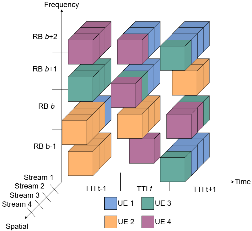
The number of antennas at the UE, denoted as , limits how many parallel data streams can be scheduled for the UE in a single RB. The number of streams per UE has to be fixed for the given TTI, i.e. it is not possible to receive different number of streams at different RB during the same TTI. This is illustrated in Fig. 1, where the number of spatial streams for the given UE and TTI is the same over all scheduled RB.
In addition, the scheduler selects an MCS index for each scheduled UE, which also has to be the same for all scheduled RB of the given UE at the given TTI. The MCS index, which is a function of received SINR (SINR), effectively defines how many data bits can be transmitted over an RB. The received SINR at a UE varies depending on the RB and on which other UE are multiplexed to the same RB. This tightly couples conventional scheduling and MCS selection.
II-A System model
We consider DL scheduling of a single 5G cell where the base station with transmitters is serving UE each having antennas. The available bandwidth is divided into RB which consist of 12 subcarriers. The scheduling decision is done for each TTI consisting of 14 OFDM (OFDM) symbols. We assume ZF (ZF) precoding for canceling both intra- and inter-user interference from the multiplexed UE. To enable simple spatial separation of the transmitted streams, each UE estimates its DL channel matrix, calculates its SVD (SVD), and feeds back the equivalent channel matrix to the base station. The SVD of th UE’s channel matrix at subcarrier and OFDM symbol is given by
| (1) |
where and are unitary matrices and is a diagonal matrix of singular values. We assume that each UE multiplies its received signal by combining matrix . The post-combining equivalent channel matrix is then given as
| (2) |
When has full rank, has nonzero entries, and it is possible to receive up to parallel data streams at each UE.
The SVD of each UE’s channel matrix effectively converts the MU-MIMO system into a MU-MISO system with virtual single-antenna users [23]. For the rest of the paper, we use virtual user indexing that maps the th data stream of the th UE into virtual user such that
| (3) |
with , and . A box in Fig. 1 represents a virtual user. The received signal of th virtual user corresponding to the th stream of UE is then
| (4) |
where is the equivalent channel vector for virtual user , is the vector of transmitted precoded symbols, is the effective additive noise term, is the th singular value of the channel matrix for UE , and is the th right singular vector of UE k. The subcarrier and OFDM symbol indexing have been left out for brevity.
Let us assume the scheduler has selected a set of virtual users , with
| (5) |
to be multiplexed to RB . In Fig. 1, the boxes of the same color in a fixed RB can be interpreted as being virtual users associated to the same UE; the constraint that only virtual users of the same UE can be included in still holds. Similar to [5], we assume constant fading within an RB. The combined effective channel matrix for those virtual users in the selected set can be given as
| (6) |
The transmitted symbol vector is then
| (7) |
where is the precoding matrix with transmit power constraint and is the vector of data symbols with . ZF precoding over the equivalent channel matrix with equal power allocation results in equal post-combining SNR for all the UE multiplexed into the same RB [23]. The post-combining SNR for each virtual user in at RB b can be given as
| (8) |
The scheduler also selects an MCS index out of possible indices for a UE based on the SNR values at the RB the UE has been scheduled. Each MCS index corresponds to a certain number of data bits per RB [24]. Given the MCS index for UE k, the number of data bits at RB for the virtual user is given by
| (9) |
where is the minimum SNR at which the UE can still successfully decode the data bits for MCS index . To simplify the analysis, the retransmissions are not considered in this study.
II-B Problem definition
The scheduling problem can be formulated as binary optimization by introducing binary decision variables, and . is a binary matrix indicating when virtual user is scheduled at RB . Similarly, is a binary matrix indicating when MCS index is selected for UE . The MU-MIMO scheduling problem can be formulated as
| (10a) | ||||
| s.t. | (10b) | |||
| (10c) | ||||
| (10d) | ||||
| (10e) | ||||
where is the per-UE scaling term for fairness. Constraint (10b) ensures that the total number of streams does not exceed the number of transmitters at the base station. Constraint (10c) is to guarantee that only one MCS index is used for a UE. Either Constraint (10d) or (10e) has to be fulfilled, which ensures the same number of streams is selected for a UE whenever multiple RB are scheduled for that UE. Note that unlike Constraint (10b), Constraints (10c) and (10d) are not based on physical radio propagation limitations, but they are rather 5G system design choices to keep the DL control signaling overhead and UE receiver complexity low. For example, assuming that Constraint (10c) is removed would result in control signaling overhead that would scale linearly with the number of RB. In addition, the UE processing complexity would increase due to decoding multiple transport blocks and potentially handling multiple parallel retransmissions per time slot.
II-B1 MU-MISO
II-B2 SU-MIMO
In the SU-MIMO case the post-combining SNR for UE depends only on the number of streams allocated for that UE. If we assume that the singular values in are in descending order, the SU-MIMO post-combining SNR for UE at RB can be given as
| (11) |
The number of data bits per UE now scales linearly with the number of data streams:
| (12) |
Let be a matrix indicating when data streams are scheduled for UE . The SU-MIMO scheduling problem can then be given as
| (13a) | ||||
| s.t. | (13b) | |||
| (13c) | ||||
| (13d) | ||||
where Constraint (13d) guarantees that the same number of data streams is selected for a UE for all RB scheduled for it.
II-C Algorithms
In this section, the optimal brute force search algorithms and several sub-optimal variants are discussed for the scheduling problem. The calculation of the SNR values is essentially the same for all the algorithms, and its complexity is not included in the analysis.
II-C1 MU-MIMO
Solving the MU-MIMO scheduling problem by exhaustive search is an extremely complex problem. The search should go through all combinations of MCS and data stream assignments for each RB. The search space size is presented as in [5]. However, if the scheduled number of data streams for user is , there are ways to select the scheduled virtual UE for that user, and the optimal selection depends on which other users are scheduled on the same RB. Thus, the actual search space is larger than that presented in [5]. In practice, once is fixed in the outer loop, the scheduler has to go through all the possible sets fulfilling Constraints (10d) or (10e).
The search space size would be exactly if only the first virtual UE of user are considered for scheduling when and . This suboptimal algorithm is expected to perform well when . The complexity can be reduced by choosing the MCS indices for the users only after the scheduling decision is made. In this sub-optimal algorithm, the best is first searched for each RB. Then for each UE, the largest MCS index resulting in non-zero data rate for all RB scheduled for the given UE, is selected. In this case, the search space size reduces to .
The complexity of the MU-MIMO scheduling problem can be further reduced by the greedy algorithm that schedules an RB to the virtual UE set with the highest rate at that RB. This fixes the number of data streams for the users in the scheduled virtual UE set. Any further scheduling decisions must fulfill the data stream requirements given in Constraints (10d) and (10e). Let be the set of all possible sets , i.e. all possible virtual UE allocations within RB. The number of possible virtual UE allocations is
| (14) |
where the last two terms ensure that only the SU-MIMO allocations with the highest SNR are included. The allowed virtual UE allocations for the given user and the given number of data streams are denoted by , . The greedy MU-MIMO scheduling algorithm is given as
Algorithm line 34 effectively reduces the search space whenever a new user is scheduled and guarantees that the data stream constraint is fulfilled for the given user. In the worst case, all the RB are scheduled for the same user and all combinations of virtual UE allocations for the other users must be considered at each iteration, which results in the worst-case search space size of .
II-C2 MU-MISO
The MU-MISO scheduling problem can be solved by going through all possible combinations of MCS assignments, and then finding which set achieves the highest data rate when scheduled for the given RB . The complexity of this brute force approach grows exponentially with as the search space size becomes .
As can be up to 29 in 5G [24], a straightforward way to reduce the complexity is to select the per-UE MCS index only after the scheduling decision is done. In this sub-optimal algorithm, the best is first searched for each RB. Then for each UE, the largest MCS index resulting in non-zero data rate for all RB scheduled for the given UE, is selected. The search space size reduces to only .
II-C3 SU-MIMO
Like the MU-MISO scheduling problem, the SU-MIMO scheduling problem can be solved by going through all possible combinations of per-UE data stream allocations and MCS assignments, and then finding which UE achieves the highest data rate when scheduled for the given RB. The complexity of the brute force approach again grows exponentially with as the search space size is . In practice the search space can be somewhat reduced because only the MCS indices in the range should be considered for UE with the given number of data streams. The minimum and maximum relevant MCS indices for UE with data streams fulfill
| (15) |
and
| (16) |
respectively. Like the MU-MISO case, the MCS indices can be decided only after the scheduling decision is made. This sub-optimal approach results in the search space size of .
The complexity of the SU-MIMO scheduling can be further reduced by the greedy approach where an RB is scheduled to the UE with the highest rate at that RB. The first RB scheduled for a UE decides the number of data streams for that UE and fixes the value of . The greedy SU-MIMO scheduling algorithm is given below
Algorithm line 22 ensures that the same RB is scheduled to only one UE. Line 23 ensures that the same number of data streams is allocated for the scheduled UE over all RB. When the search is done only over the non-zero elements of , the search space reduces at each iteration of the while loop. The search space size for the greedy SU-MIMO scheduling algorithm is in the worst case. The worst case occurs when the first RB are all scheduled to the same UE.
III QUBO formulation of the problem
In resource allocation or scheduling problems formulated as QUBO we have binary decision variables , , one variable for each resource unit decision. We use the notation for the index set with cardinality . We consider a mathematical expression of the form
| (17) |
and we want to find the vector that minimizes the expression (17). The elements of the matrix are coefficients that depend on the problem.
Optimization problems usually have constraints. If the constraints can be reformulated as quadratic penalty terms of the binary variables, the constraints are embedded in QUBO and we are in the ’unconstrained’ situation. The constraints can reduce the set of solutions or make it harder to find any.
III-A MU-MIMO
First, we briefly consider a QUBO approach to the general MU-MIMO problem. Recall that the numbers , , , and are parameters. Only , the number of UE, is variable. The number of virtual streams is . If , then each virtual stream could have its own . If , then all virtual streams cannot be allocated in the same time slot TTI.
The term in (10a) requires a careful approach, since the rate in RB depends on all users (virtual streams) that are allocated to this , the set , which is a subset of the th column of the matrix . This means that, for a fixed resource block , we should study products of binary variables of the form
| (18) |
and if this leads to problems of higher-order than quadratic. The order of the MU-MIMO scheduling problem can be as high as where the additional dimension comes from the MCS index decision variable . Even though there are systematic procedures available for converting higher-order problems to quadratic [10], the number of additional auxiliary variables soon becomes very high for .
The MU-MIMO scheduling problem would be relatively straightforward to formulate as QUBO if Constraints (10c), (10d), and (10e) could be relaxed. These constraints are per-UE over all the RB while our approach in the MU-MIMO case first converts the system into the MU-MISO system with virtual users. This makes the proper formulation of the constraints as quadratic penalties difficult. Because of these challenges and the high-order of the binary optimization problem, we focus in this paper on the simpler MU-MISO and SU-MIMO cases.
III-B MU-MISO
A straightforward way to formulate the MU-MISO scheduling problem as quadratic binary optimization would be to introduce a binary matrix indicating which of the UE sets in is scheduled for a given RB. The number of different UE sets in the MU-MISO case is
| (19) |
The mapping of the binary decision variables to and would then be
| (20) |
The elements of the QUBO matrix can be expressed with the help of (9) as
| (21) |
where , , , and .
The MU-MISO scheduling problem is constrained by the fact the only a single UE set can be scheduled for an RB and by (10c). When rewriting them using the QUBO variables we get
| (22) |
and
| (23) |
Constraints (22) and (23) can be converted to quadratic penalty terms by using a simple transformation from [8]. The resulting QUBO problem can be given as
| (24) |
where is the final QUBO matrix including the penalty terms. The number of QUBO variables is .
III-C SU-MIMO
The SU-MIMO scheduling problem (13a) has three binary decision variable matrices , , and that can be mapped into HUBO (HUBO) variables as
| (25) |
The SU-MIMO scheduling problem is of the third order with the HUBO coefficients from (12)
| (26) |
where , , , and .
Since most solvers can work only on QUBO problems directly, we first convert the HUBO problem into a constrained quadrature binary optimization problem. This conversion can be done by quadratization using the Rosenberg’s procedure [10]. Let be the function to be minimized with third-order monomials. The quadratization can be done iteratively as
- 1.
Select two variables and such that their product is the most common among the monomials of degree at least 3 in .
- 2.
Let be the function obtained upon replacing each occurrence of by a new variable in .
- 3.
Let , where is large enough positive number.
- 4.
Let . If the order of is higher than two, go to step 2.
In the SU-MIMO case to simplify the constraint mapping, we restrict the Rosenberg’s procedure such that only and , where and , are selected for variable pairs. This can be interpreted such that auxiliary variable corresponds to scheduling RB to UE with data streams. The number of auxiliary variables after the quadratization procedure is finished is and the total number of variables is . In practice, the SNR distribution is often such that no data can be transmitted with the highest MCS indices, even with a single stream. Using (16), we define the highest feasible MCS index for UE as when . To reduce the number of QUBO variables, only the MCS indices can be considered for UE . In this case, the number of QUBO variables is .
The QUBO variable vector after quadratization is given as
| (27) |
where the auxiliary variables are organized RB-by-RB, i.e. the first elements after correspond to RB 1 and the last elements in correspond to RB . The monomial coefficients are collected to matrix after quadratization.
The linear constraints to the SU-MIMO binary optimization problem are given in (13b), (13c), and (13d). In addition, there is an additional constraint for the auxiliary variables ensuring that only one user-number of streams pair is selected per RB:
| (28) |
where . Using the same transform as in Section III-B for converting linear constraints to quadratic penalties, the QUBO problem becomes
| (29) |
IV Numerical results
In order to verify the correctness of the QUBO formulations from Section III and to compare the complexity-performance trade-off of scheduling algorithms from Section II-C, we simulate the system with the assumptions given in Table I. As already mentioned in Section II-A, constant fading is assumed within an RB. We denote the channel matrix for user at RB and TTI as .
| MCS table | Table 5.1.3.1-2 [24], |
|---|---|
| SNR thresholds | where is the spectral |
| efficiency from Table 5.1.3.1-2 [24] for MCS | |
| Transmitted SNR | |
| Fading assumptions | where |
| , , | |
| , , | |
| , | |
| uncorrelated spatial fading | |
| Number of TTI | |
| Proportional | Scaling at TTI |
| fairness | where |
| is the number scheduled data bits for | |
| user at previous TTI | |
| Traffic assumptions | Per-user DL buffers never emptied |
| All traffic with the same priority |
IV-A Empirical evaluation of the correctness of the QUBO formulations
A straightforward way to verify the correctness of the QUBO formulations from Section III would be to compare their solutions to the results from the corresponding optimal brute force algorithms of Section II-C. However, this approach is infeasible in practice as the number of QUBO variables grows beyond the capabilities of any optimal QUBO solver. In addition, it soon becomes infeasible to obtain the optimal solutions from the brute force algorithm due to long execution time when . For cases where , it is possible to evaluate the correctness of the QUBO matrices with the two tests: 1) When the brute force solution is converted to binary vectors and multiplied with the QUBO matrix as , we should get exactly the same result as the value of the objective function from the brute force search, and 2) Sub-optimal QUBO solvers should never get better results than the brute force search.
When going through all the parameter pairs and , the multiplication in the first test resulted in the same value as the optimal objective function value for all cases. For the second test, the formulated QUBO is solved using the simulated annealing and simulated quantum annealing algorithms from D-Wave Ocean SDK [25].
The parameters for solving the QUBO problems are given in Table II. Different parameter values were tested until a set that worked fairly well with simulated annealing algorithms was found. The quadratization penalty was set to a slightly larger value than the maximum number of data bits for an RB with a single data stream. The constraint penalty was set to scale with like the optimal solution as recommended in [8]. The simulated annealing algorithms were not very sensitive to the selection of the constraint penalty as long as the penalty was large enough. This is illustrated in Fig. 2 where the number of scheduled data bits per TTI are shown as a function of (the same is used for all constraints) for SU-MIMO when and . It can be seen that the constraints are violated, which is visible as solutions exceeding the optimum value, when too small penalty values are used. An example QUBO matrix presented as a heat map is shown in Fig. 3. The dark orange elements correspond to the penalties from the constraints, while the other elements result from the quadratization procedure.
| Penalty for constraints | , , MU-MISO |
|---|---|
| , , SU-MIMO | |
| Quadratization penalty (SU-MIMO) | |
| Temperature range and schedule | Default, set by Ocean SDK |
| Number of reads | 500 |
| Number of sweeps | |
| Number of sweeps per temperature | 2 |

The results of the QUBO formulation evaluation are shown Figs. 4 and 5 where solutions for a single TTI are shown for MU-MISO and SU-MIMO, respectively. The number of base station transmitters is fixed to for both cases, and the number of receiving antennas is fixed to for the SU-MIMO case. It can be seen that simulated annealing is able to achieve close-to-optimal solutions. In addition, the solutions from the simulated annealing should never exceed those from the brute force search, which is the case in Figs. 4 and 5. This, together with the results from the first test, gives us confidence that the QUBO matrices in (24) and (29) are correctly formulated. The number of QUBO variables as a function of the number of RB is also shown as red lines. This illustrates that the number of QUBO variables increase linearly with the increasing bandwidth (number of RB) for both MU-MISO and SU-MIMO.
The scaling of the problem search space size and the number of QUBO variables are shown in Fig. 6 as a function of the number of users when . This illustrates the problem complexity increases exponentially as grows for both MU-MISO and SU-MIMO cases. The QUBO formulation of the MU-MISO scheduling problem is practical for only a small number of users as the number of required QUBO variables grows polynomially with . On the other hand, the number of QUBO variables grows only linearly with the SU-MIMO QUBO formulation.
Although the SU-MIMO QUBO formulation looks promising in terms of the number of QUBO variables, the coupling between the variables can be problematic for quantum implementation. To study this further, we formulated the SU-MIMO QUBO matrices as logical graphs and attempted to embed them into the topologies of the current state-of-the-art D-Wave quantum annealers. The results indicate that even though the embedding can be done when both the number of UE and RB are low, some of the logical QUBO variables have to be represented by long chains of physical qubits. This makes the practical implementation of the SU-MIMO scheduling infeasible with the current state-of-the-art quantum annealers, see Appendix A for details. However, the qubit connectivity has been improving with each new topology. If the same trend continues, embedding to the future quantum annealers should be easier with shorter chain lengths.
IV-B Complexity and performance of the scheduling algorithms
Based on the scalability analysis, the SU-MIMO QUBO formulation looks promising for further study because the number of QUBO variables grows only linearly while the problem search space grows exponentially. However, even if we had a quantum solver capable of solving the SU-MIMO problem optimally with a high probability, a relevant question is whether solving the SU-MIMO problem is worth the effort. In other words, how close to optimum we can get with the low-complexity sub-optimal algorithms.
To get a better understanding of this question, we analyze the sub-optimal algorithms presented in Section II-C3 in terms of their complexity and performance. The considered algorithms are the exhaustive brute force search, the brute force search with Constraint (13c) relaxed and MCS indices decided after scheduling, and the greedy search. The algorithms are labeled as ’Brute force’, ’No MCS’, and ’Greedy’ in the figures of this section, respectively.
The algorithm complexity is presented as the search space size assuming that all MCS indices are included in the search for all UE. The search space size is shown as a function of number of RB and number of UE in Fig. 7, (7a) and (7b), respectively. As explained in Section II-C3, the search space size is random for the greedy algorithm, and thus each point for the greedy algorithm represents an average over 100 time slots; the variability of the average is not visible on the logarithmic scale. The search space size of the greedy algorithm grows only linearly with , which makes it a potential option for real-time scheduling at each time slot.
The performance of the SU-MIMO algorithms in terms of the sum rate over 100 time slots as a function of number of RB is shown in Fig. 8. As expected, the brute force algorithm performs best while the greedy algorithm achieves the lowest sum rate. The sum rate curves do not increase monotonically because the path loss terms in the channel matrix (see Table I) are randomly drawn from the uniform distribution for each value of causing considerable variation in the ’goodness’ of the UE locations.
To make it easier to interpret the gain of using the optimal brute force algorithm, the sum rate gain relative to the greedy algorithm is shown in Fig. 9. The performance gain of using the optimal brute force algorithm compared to the greedy algorithm when is 10-40% with the growing trend with respect to the number of RB.
When the number of UE considered for scheduling increases, the performance gap between the greedy and brute force algorithms decreases. This is illustrated in Fig. 10 where the sum rate gain relative to the greedy algorithm is shown for several values of when . We had to limit the number of UE up to because the brute force algorithm run times grow very long with higher values of . For example with , , , the search space size is . Even if the gain from the optimal brute force algorithm is small for large in a single time slot, the cumulative effect of being able to serve more traffic and to keep the user-experienced quality of service high might still be notable in the long term.
The performance results in this section indicate that the gain from solving the SU-MIMO scheduling optimally is largest when the number of scheduled UE is small and the number of RB is large. Assuming that we had a working quantum solver for the QUBO problem available, it would make sense to pre-evaluate the limits for the pair of parameters and to decide when to use the QUBO-based optimum solver and when a suboptimal low-complexity algorithm, such as the greedy search.
V Conclusion
We have formulated the DL MU-MISO and SU-MIMO scheduling problems in 5G base stations as QUBO and analyzed their scalability in terms of the number of required QUBO variables. In particular, the SU-MIMO QUBO formulation looks promising for further study as the number of QUBO variables grows only linearly as a function of number of users while the problem search space size grows exponentially. This is important as there can be tens of users considered for scheduling in the network during the rush hours.
In addition, we analyze the complexity-performance trade-off of suboptimal scheduling algorithms, which provides insight into when solving the problem optimally using quantum computers may be useful in practice. The results indicate that the gain from solving the SU-MIMO DL scheduling problem optimally is largest when the number of resource blocks is large and the number of users is small. In practice, either a QUBO-based optimum solver or a suboptimal low-complexity algorithm could be selected based on system parameters.
Our initial embedding study shows that it is not yet feasible to embed the SU-MIMO QUBO graphs to the current state-of-the-art D-Wave quantum annealers when the number of resource blocks is 70 or larger. In addition, the chain lengths after embedding are so long that it would be very unlikely to get close-to-optimal solutions from the current annealers. However, our results can be used as a starting point for alternative and potentially more practical QUBO formulations of the scheduling problem as well as for quantum implementations. A potential future work could to be to apply the QUBO approach only on MU-MIMO subproblems such as virtual user selection.
Appendix A Embedding to D-Wave topologies
To evaluate the practical feasibility of applying the proposed QUBO formulations on current quantum annealers, we study the minor embedding of the QUBO matrices derived in Section III onto D-Wave hardware topologies. Embedding maps the logical QUBO variables to the physical qubits of the given quantum processing unit topology. Because the practical qubit topologies are not fully connected, some of the logical variables must be represented as a chain of physical qubits. Longer chains are generally undesirable because they increase the likelihood of chain breaks reducing the quality of the solutions returned by a quantum annealer [26].
We focus on the SU-MIMO case, which is the most interesting for practical implementation due to the linear scaling of the number of QUBO variables. In addition for the rest of this section, we assume . QUBO matrices from (29) can be represented as logical QUBO graphs where each binary variable corresponds to a vertex and an edge is added between variables and whenever . Before actual embedding, its difficulty can be estimated by evaluating the QUBO graph degree and density. The summary of the results from the QUBO graph analysis is collected to Table III. The values are the averages from 100 individual channel realizations per each pair. This approach was selected because, as discussed in Section III-C, there is some variation in the number of logical QUBO variables due to the variation in the number of feasible MCS indices. It can be seen from Table III that the the graph density decreases as both and increase. In addition, the average degree increases only slightly with the increasing problem size. This indicates that the QUBO graphs remain relatively sparse as the problem scales, which is favorable for minor embedding onto quantum annealing hardware. However, the maximum degree of the graphs is high. This necessitates the use of long chains of physical qubits with real-life quantum annealer topologies.
| Graph density | Avg. degree | Max. degree | ||||
| 2 | 20 | 246 | 3145 | 0.104 | 25.5 | 95.2 |
| 2 | 30 | 346 | 4474 | 0.0749 | 25.8 | 132 |
| 2 | 40 | 447 | 5991 | 0.0599 | 26.8 | 171 |
| 2 | 50 | 547 | 7435 | 0.0496 | 27.1 | 209 |
| 2 | 60 | 647 | 8665 | 0.0415 | 26.8 | 245 |
| 2 | 70 | 747 | 9969 | 0.0358 | 26.7 | 280 |
| 3 | 20 | 369 | 5226 | 0.0769 | 28.3 | 97.3 |
| 3 | 30 | 519 | 7505 | 0.0558 | 28.9 | 135 |
| 3 | 40 | 669 | 9866 | 0.0440 | 29.4 | 173 |
| 4 | 20 | 492 | 7661 | 0.0634 | 31.1 | 99.2 |
| 4 | 30 | 692 | 11079 | 0.0463 | 32.0 | 137 |
| 5 | 20 | 612 | 10186 | 0.0544 | 33.3 | 98.1 |
The target topologies for embedding are selected as Pegasus and Zephyr that correspond to D-Wave Advantage and Advantage2 quantum annealers, respectively [27]. A logical QUBO graph is randomly selected from the 100 generated graphs for each pair. The logical QUBO graphs are embedded onto the target topologies using the find_embedding function of the Ocean SDK minorminer library. The find_embedding function is an implementation of the heuristic algorithm for finding graph minors presented in [28]. Because the minor embedding algorithm is heuristic, we repeat the embedding 10 times for each QUBO graph and select the best embedding with the lowest qubit count. For each successful embedding, the number of needed physical qubits, the median chain length, and the 75th and 95th percentile of the chain length are collected to Tables IV and V for the Pegasus and Zephyr topologies, respectively. In general, the Zephyr topology with the improved qubit connectivity achieves shorter chain lengths than the Pegasus topology. Unfortunately, for both topologies and for all the tried pairs there are many long chains. This either requires the use of high chain strengths or increases the probability of chain breaks, both of which significantly decrease the probability of achieving close-to-optimal solutions [26]. When or increases, the embedding can no longer be done because there are not enough physical qubits available. This happens e.g. when and .
| Qubits | Chain length | Chain length | Chain length | ||||
| median | P75 | P95 | |||||
| 2 | 20 | 247 | 3224 | 1601 | 5 | 8 | 15 |
| 2 | 30 | 336 | 3417 | 2328 | 5 | 7 | 25 |
| 2 | 40 | 449 | 6367 | 3885 | 6 | 9 | 30 |
| 2 | 50 | 543 | 6495 | 4313 | 5 | 7 | 37 |
| 2 | 60 | 642 | 7622 | 4819 | 4 | 6 | 40 |
| 2 | 70 | 750 | 10536 | N/A | N/A | N/A | N/A |
| 3 | 20 | 367 | 5055 | 3745 | 9 | 14 | 22 |
| 3 | 30 | 506 | 6121 | 4668 | 5 | 8 | 42 |
| 3 | 40 | 667 | 9410 | N/A | N/A | N/A | N/A |
| 4 | 20 | 497 | 8027 | N/A | N/A | N/A | N/A |
| Qubits | Chain length | Chain length | Chain length | ||||
| median | P75 | P95 | |||||
| 2 | 20 | 247 | 3224 | 1345 | 5 | 7 | 12 |
| 2 | 30 | 336 | 3417 | 1782 | 4 | 5 | 20 |
| 2 | 40 | 449 | 6367 | 3136 | 4 | 6 | 33 |
| 2 | 50 | 543 | 6495 | 3438 | 4 | 5 | 34 |
| 2 | 60 | 642 | 7622 | 3938 | 4 | 5 | 29 |
| 2 | 70 | 750 | 10536 | N/A | N/A | N/A | N/A |
| 3 | 20 | 367 | 5055 | 3236 | 7 | 11 | 24 |
| 3 | 30 | 506 | 6121 | 3792 | 5 | 7 | 34 |
| 3 | 40 | 667 | 9410 | N/A | N/A | N/A | N/A |
| 4 | 20 | 497 | 8027 | N/A | N/A | N/A | N/A |
Acknowledgment
The authors want to thank Hannu Reittu for his early assistance with the QUBO formulations, Kari Seppänen for CPLEX testing, Prof. Animesh Yadav for many fruitful discussions on the research topic, and Costantino Carugno and Andrea Marchesin for help and feedback in quantum annealing questions.
References
- [1] 3GPP TS38.212, “NR; Multiplexing and channel coding V17.11.0.” 3GPP, Technical Specification, 2025.
- [2] E. Castañeda, A. Silva, A. Gameiro, and M. Kountouris, “An overview on resource allocation techniques for multi-user MIMO systems,” IEEE Commun. Surveys Tuts., vol. 19, no. 1, pp. 239–284, 2017.
- [3] G. Femenias, F. Riera-Palou, X. Mestre, and J. J. Olmos, “Downlink scheduling and resource allocation for 5G MIMO-Multicarrier: OFDM vs FBMC/OQAM,” IEEE Access, vol. 5, pp. 13 770–13 786, 2017.
- [4] J. De Luna Ducoing and K. Nikitopoulos, “Scalable MU-MIMO user scheduling for next-generation wireless networks,” in Proc. IEEE CAMAD, Edinburgh, UK, Nov. 2023, pp. 19–24.
- [5] Y. Chen, Y. Wu, Y. T. Hou, and W. Lou, “mCore+: A real-time design achieving 500 s scheduling for 5G MU-MIMO systems,” IEEE Trans. Mobile Comput., vol. 22, no. 12, pp. 7249–7265, 2023.
- [6] Y. Wu, Y. Shi, Y. T. Hou, W. Lou, J. H. Reed, and L. A. DaSilva, “R³: A real-time robust MU-MIMO scheduler for O-RAN,” IEEE Trans. Wireless Commun., vol. 23, no. 11, pp. 17 727–17 743, 2024.
- [7] F. Chicano, G. Luque, Z. A. Dahi, and R. Gil-Merino, “Combinatorial optimization with quantum computers,” Engineering Optimization, vol. 57, no. 1, pp. 208–233, 2025.
- [8] F. Glover, G. Kochenberger, and Y. Du, “Quantum bridge analytics I: A tutorial on formulating and using QUBO models,” 4OR, vol. 17, no. 4, pp. 335–371, 2019.
- [9] D. Volpe, G. Orlandi, and G. Turvani, “Improving the solving of optimization problems: A comprehensive review of quantum approaches,” Quantum Reports, vol. 7, no. 1, 2025.
- [10] M. Anthony, E. Boros, Y. Crama, and A. Gruber, “Quadratic reformulations of nonlinear binary optimization problems,” Mathematical Programming, vol. 162, pp. 115–144, 2017.
- [11] G. Barillaro, A. Boella, F. Gandino, M. G. Vakili, E. Giusto, G. Mondo, B. Montrucchio, A. Scarabosio, A. Scionti, O. Terzo, and G. Vitali, “Comparison of heuristic approaches to PCI planning for quantum computers,” in Proc. IEEE ICCE, Las Vegas, NV, Jan. 2023, pp. 1–6.
- [12] S. Kasi and K. Jamieson, “Towards quantum belief propagation for LDPC decoding in wireless networks,” in Proc. MobiCom, London, UK, Sep. 2020, pp. 663–676.
- [13] S. Kasi, J. Kaewell, and K. Jamieson, “A quantum annealer-enabled decoder and hardware topology for nextG wireless polar codes,” IEEE Trans. Wireless Commun., vol. 23, no. 4, pp. 3780–3794, 2024.
- [14] B. Gülbahar, “Majority voting with recursive QAOA and cost-restricted uniform sampling for maximum-likelihood detection in massive MIMO,” IEEE Trans. Wireless Commun., vol. 24, no. 3, pp. 2620–2631, 2025.
- [15] S. Winter, Y. Zhang, G. Zheng, and L. Hanzo, “A lattice-reduction aided vector perturbation precoder relying on quantum annealing,” IEEE Wireless Commun. Lett., vol. 13, no. 5, pp. 1225–1229, 2024.
- [16] K. Yonaga, K. Takizawa, and M. Inaba, “Error rate analysis of quantum-annealing-aided multi-user detection in power-domain nonorthogonal multiple access,” IEEE Access, vol. 13, pp. 56 671–56 681, 2025.
- [17] Q. J. Lim, C. Ross, A. Ghosh, F. W. Vook, G. Gradoni, and Z. Peng, “Quantum-assisted combinatorial optimization for reconfigurable intelligent surfaces in smart electromagnetic environments,” IEEE Trans. Antennas Propag., vol. 72, no. 1, pp. 147–159, 2024.
- [18] “Developing quantum computing infrastructure for service optimization: Application to base stations to optimize communications services start in july,” Press Release, NTT DOCOMO, Jun. 2024. [Online]. Available: https://www.dwavequantum.com/media/gyaje2qb/ntt-docomo-translation-of-docomo-pr.pdf
- [19] C.-H. Hsu and Z. Ding, “Variational quantum algorithm for user scheduling in broadband MU-MIMO systems,” IEEE Trans. Wireless Commun., vol. 25, pp. 1196–1208, 2026.
- [20] G. Scriva, N. Astrakhantsev, S. Pilati, and G. Mazzola, “Challenges of variational quantum optimization with measurement shot noise,” Phys. Rev. A, vol. 109, p. 032408, Mar 2024.
- [21] A. Bärligea, B. Poggel, and J. M. Lorenz, “Scalability challenges in variational quantum optimization under stochastic noise,” Phys. Rev. A, vol. 112, p. 032407, Sep 2025.
- [22] D. Volpe, G. A. Cirillo, R. Fantini, A. Boella, G. Mondo, M. Graziano, and G. Turvani, “Quantum-compliant users scheduling optimization in joint transmission mobile access networks,” Quantum Information Processing, vol. 23, no. 262, 2024.
- [23] A. Panajotović, F. Riera-Palou, and G. Femenias, “Adaptive uniform channel decomposition in MU-MIMO-OFDM: Application to IEEE 802.11ac,” IEEE Trans. Wireless Commun., vol. 14, no. 5, pp. 2896–2910, 2015.
- [24] 3GPP TS38.214, “NR; Physical layer procedures for data V17.14.0,” 3GPP, Technical Specification, 2025.
- [25] Ocean SDK. D-Wave. [Online]. Available: https://docs.dwavequantum.com/en/latest/ocean/index.html
- [26] Minor embedding: Best practices – D-Wave quantum computing products documentation. D-Wave. [Online]. Available: https://docs.dwavequantum.com/en/latest/quantum_research/embedding_intro.html
- [27] Per-QPU solver properties and schedules – D-Wave quantum computing products documentation. D-Wave. [Online]. Available: https://docs.dwavequantum.com/en/latest/quantum_research/solver_properties_specific.html
- [28] J. Cai, W. G. Macready, and A. Roy, “A practical heuristic for finding graph minors,” ArXiv pre-print, Jun. 2014. [Online]. Available: https://arxiv.org/abs/1406.2741