Towards Digital Halftoning on Closed Manifolds–An Error Diffusion Scheme for the Torus based on Sigma-Delta Quantization along the Rank-one Lattice
Abstract
Digital halftoning aims to represent continuous-tone images by binary patterns while preserving their visually relevant low-frequency content. Among the many available approaches, error-diffusion methods implement noise shaping through causal feedback filters and can be interpreted as two-dimensional versions of the signal quantization paradigm Sigma–Delta modulation. On closed domains, however, the terminal state of the underlying recurrence relation need not match the initial one, producing boundary artifacts. We study this problem for bandlimited functions on the two-dimensional torus. By arranging all pixels along a single closed rank-one lattice, we replace the multiple mismatches associated with separately processed rows and columns with a single terminal contribution, while retaining exact reconstruction. For a uniform lattice with points, we obtain first- and second-order error bounds of order and . A suitable constant update eliminates the terminal mismatch and reduces the spatial localization of the error without changing these asymptotic orders. For fixed-direction rank-one lattices, the corrected first- and second-order reconstructions instead achieve rates and . Numerical experiments illustrate a reduction in boundary artifacts compared with classical schemes applied on the Cartesian grid.
1 Introduction
Digital halftoning is the process of reproducing a continuous-tone image by means of a binary pattern of black and white pixels. Since the output contains no intermediate intensity values, gray levels cannot be represented pointwise; instead, they are created by the local density and spatial arrangement of the dots. This mechanism relies on the fact that the human visual system acts, to first approximation, as a low-pass filter and therefore averages sufficiently fine spatial variations. As a consequence, the relevant objective is not to make the representation error small at every pixel, but to control its low-frequency component, as this is sufficient for visual similarity. As the coarseness of the binary representation prevents the total error from being small, this goal needs to be achieved by the so-called noise shaping paradigm: the visually significant part of the error is reduced by moving most of its energy towards higher spatial frequencies, where it is attenuated by the visual system.
A number of algorithms explicitly build upon the idea of noise shaping. Specifically, error-diffusion algorithms (see, for example, [1, 2, 3, 4, 5]) implement this principle through a recursive feedback mechanism. The discrepancy produced at one pixel is propagated to subsequent pixels and influences their binary values, so that nearby errors tend to cancel after spatial averaging. This feedback structure is exactly analogous to the analog-to-digital (A/D) conversion scheme Sigma-Delta () modulation [6], which is why error diffusion has been interpreted in the literature as two-dimensional [7]. In this formulation, the sampled gray-scale values of the image take the role of the input to the quantizer, while the halftoned image corresponds to the -bit quantized representation, with each bit encoding whether the corresponding pixel is black or white.
That said, most of the algorithmic and theoretical developments of modulation have been achieved in the one-dimensional case. The main idea in is that an ordered sequence of samples is processed recursively and an internal state variable records the accumulated quantization error. Beginning with the work of Inose and Yasuda [6], this approach has become a standard method for coarse analog-to-digital conversion, while its mathematical analysis for bandlimited functions was initiated by Daubechies and DeVore [8] and subsequently developed to obtain exponentially accurate one-bit schemes; see, for example, [9, 10]. A notable exception to the focus on is the work [5], with its refinement [Sampta paper], which proves error guarantees for weighted combinations of schemes applied to solve the problem.
The underlying geometry in both and is, for all these papers, the standard Euclidean geometry, potentially restricted to a subset of or . However, motivated by surface printing, the digital halftoning problem is also interesting for more general manifold domains. A challenge in this general framework arises when the manifold has a non-trivial topology and hence does not have a canonical identification with subsets of or .
This issue is particularly relevant on a closed manifold, as there is no distinguished boundary at which the recursion should naturally begin or end. In , this problem has been studied in [11] with the focus on the simplest case where this issue arises, namely the circle. In order to apply a standard quantizer in this context, one needs to designate a starting point for the recurrence relation, which is then also the endpoint. Consequently, one can encounter a mismatch of the state variable at this point, which translates into an additional local reconstruction error in the neighborhood of the endpoint. As shown in [11], this is not just an artifact of the algorithm, but the error decay for a large oversampling rate is provably worse than in the Euclidean case. This problem has also been investigated in the more general framework of finite frames; see [12, 13, 14, 15, 16]. In this setting, eliminating the boundary contribution generally requires a non-translation-invariant dual: the reconstruction kernel has to be chosen depending on the sample location, which is not in line with the model commonly assumed for human vision.
As a remedy, [11, 17] suggest not representing the original image but rather a perturbation of it obtained by adding a small constant. The motivation is that adding a small global constant is visually preferred over a local perturbation of the same magnitude. If the constant update is chosen carefully, the updated signal can be represented with provably better error decay.
In , a natural analog to the circle is the torus. However, applying the results of [5] requires not just a small number of initial conditions, but one needs to initialize the state variables at an entire vertical line and at an entire horizontal line, so the question of how to correct the boundary error is considerably more involved than in .
In this paper, we address this issue by replacing the collection of row-wise orderings by a single trajectory containing all the sampling points. This allows us to then extend the program initiated in [11], where one-bit quantization on the circle was considered as a first model for error propagation on closed manifolds.
The idea of using a curve to impose a one-dimensional ordering on an image has already appeared in digital halftoning, notably through space-filling curves and related error-diffusion algorithms [15, 18]. In those works, the curve is primarily used as an algorithmic device for scanning the pixels and reducing directional artifacts. Here, instead, the trajectory is chosen so as to be compatible with both the topology of the torus and the Fourier reconstruction of the image.
Our trajectory of choice is a line on the torus, chosen such that the corresponding samples form a so-called rank-one lattice (see [19, 20, 21] for more details), which has recently played an important role in the construction of variants of the Fast Fourier Transform. More precisely, we sample the image on a rank-one lattice with points. As its nodes all lie on a line, they can be processed by one unchanged one-dimensional recursion. The particular choice also makes the lattice spatially uniform: its points are the centers of congruent rotated square pixels that partition the entire torus. At the same time, the lattice is reconstructing for the prescribed bandlimited space (see Section of [19]), which leads to an exact equal-weight sampling formula. Thus, the same construction provides a closed ordering for quantization, a uniform pixelization of the torus, and an exact reconstruction operator.
Since all samples belong to a single trajectory, a boundary mismatch only occurs in a single point. In addition, this mismatch is small, as the size of this mismatch is inversely proportional to the sequence length. Even without any update, this favorable effect of the sequence length allows for first and second-order errors given by
After a constant correction, in the spirit of the result, one can further improve this scaling. However, this requires changing the discretization geometry and representing the image by rectangular pixels, rather than square ones. For that, we fix a line of large enough slope and increase the number of samples on that fixed trajectory. In this scenario, the reconstruction error scales as
for the first and second-order schemes, respectively. This gives a trade-off between spatially uniform pixels and faster asymptotic decay.
2 Preliminaries
We begin by introducing the signal model and the main properties of quantization that will be used throughout the paper. As a guiding example for a two-dimensional closed manifold domain, we consider the torus, so we study functions on the two-dimensional torus . Motivated by the fact that human vision can be modeled as a low-pass filter (as discussed in the introduction), we assume that the perceived images that we aim to approximate are bandlimited on that domain. This assumption is directly aligned with A/D conversion theory, where it models the fact that different classes of signals occupy different frequency bands, and signal components outside the band of interest can be suppressed by a band-pass filter. To fully exploit this analogy, we represent the gray values by the symmetric interval , where corresponds to black and to white.
Instead of , we work with with opposite sides identified and regard functions on as functions on that are -periodic in each variable. For , we use the normalization
| (1) |
where . With this notation, the bandlimited images considered in this paper belong to the following function space
| (2) |
which can be interpreted as the periodic analog of the Paley-Wiener space
Equivalently, the signal model is the class of trigonometric polynomials with exponents contained in the square . It is well known that in this framework, an analog of Shannon’s sampling theorem can be formulated using the Dirichlet kernel (Reference to book). More precisely, let , and let be the samples of on the Cartesian grid , with . Then can be exactly recovered from these samples as
| (3) |
where , and is the Dirichlet kernel of bandwidth ,
| (4) |
Hence, before quantization, the finite array fully represents the bandlimited function . This exact sampling identity is the starting point for the quantization problem.
The goal is now to replace the gray values by black and white or, equivalently, the real-valued samples by quantized values in such a way that is well approximated by
| (5) |
That is, we aim to control the reconstruction error , which can be expressed via (5) and (3) as
| (6) |
Thus, the reconstruction error is obtained by applying the low-pass reconstruction kernel to the quantization error . The aim is to choose the quantized values so that becomes small as the oversampling rate increases.
For such a coarse alphabet, just rounding the samples would not yield a meaningful representation; for example, all positive signals would be represented by the same array containing only the value . By contrast, quantization chooses the quantized values in an interdependent way, in such a way that the quantization error is close to the null space of the low-pass reconstruction kernel. In other words, the error is shaped to be high-pass, which is why this paradigm is known as noise-shaping.
We briefly recall the one-dimensional framework underlying the analysis of quantization, following [8]. Let and suppose that is sampled at rate . Then can be represented using a smoothed low-pass kernel given by a Schwartz function satisfying
via the equality
| (7) |
Replacing the samples by one-bit values gives the quantized reconstruction
| (8) |
and hence
| (9) |
Thus, the reconstruction error is obtained by applying a low-pass filter to the sample-wise quantization error . The insight of quantization is that if that error can be expressed as the finite difference of a bounded state variable, one can exploit the smoothness of the kernel to control the reconstruction error. More precisely, denoting by the backward difference operator,
an -th order scheme is driven by a state sequence defined via the equality
| (10) |
Substitution into (9), followed by discrete summation by parts, transfers the differences from the state sequence to the reconstruction kernel and yields the standard estimate
| (11) |
see [8]. In particular, a uniform bound on the state sequence leads to -th order decay of the reconstruction error as the oversampling rate increases.
A key ingredient for our method is the class of generalized schemes described by a causal feedback filters with . Given an ordered input sequence , the quantization rule is
| (12) |
where and denotes the internal state updated by the recursion. Following [9], such a scheme yields a similar -th order error decay if there exists such that
| (13) |
Indeed, the recursion gives
and therefore the reparametrized state satisfies
Combining this relation with (11) gives
| (14) |
The reconstruction accuracy is therefore governed by two quantities: the size of the implemented state and the norm . A scheme is said to be stable if remains uniformly bounded, independently of the length of the input sequence. This property is essential for obtaining reconstruction guarantees, since enters directly into the corresponding error estimate.
A standard sufficient condition for stability is
| (15) |
If the initial states lie in , this condition guarantees that ; see [9]. It has been demonstrated empirically that optimizing the filters in view of conditions (14) and (15), gives rise to sparse filters . This has motivated the study of filters of minimal support, namely, filters with the smallest number of nonzero coefficients compatible with the prescribed order; see [9, 22]. In the first-order case, the only such filter is given by , for the second order, these filters are given by
| (16) |
where has length and only two nonzero coefficients. Since
the sufficient stability condition above is satisfied whenever
The choice of filter must therefore balance the stability requirement with the control of , which determines the constant in the reconstruction estimate.
Minimally supported filters have been the key ingredient of the weighted schemes for -dimensional signals proposed in [5], and they will also play a key role in this paper.
3 Boundary effects of Sigma-Delta schemes on manifolds
In the -dimensional torus, fixing one coordinate of a bivariate bandlimited function produces a one-dimensional bandlimited function of the remaining variable. Each row or column of the Cartesian sampling grid can therefore be regarded as the sampling of a bandlimited signal on the circle. Coarse quantization in such a scenario has been studied in [11].
That work observes that applying in this context gives rise to boundary effects near the point where the scheme is initiated. These effects are not specific to , but in general, unavoidable: the paper shows that there exist bandlimited signals—in fact, even constant signals—for which the periodic reconstruction error is bounded from below by a multiple of , independently of how the binary values are assigned to the samples. The obstruction is therefore not tied to a particular quantization rule. It reflects the fact that a finite binary sequence does not, in general, close consistently when interpreted as the quantization of a signal on the circle.
This mechanism is particularly relevant for second-order schemes. Away from the endpoints, second-order noise shaping produces the expected quadratic cancellation. Terminal contributions, however, may remain on the scale and can therefore dominate the interior contribution. This problem can be avoided when the signal is altered by adding a suitable constant (which, arguably, is less severe than a non-constant error of comparable size), see [11]. Under an appropriate stability assumption, this modification yields second-order accuracy with respect to the shifted signal.
In , however, the suitable alterations can differ from line to line and column to column, and it is not clear how a global benign alteration can be designed. Without such an alteration, one can still phase boundary effects, but this time on boundary, rather than just a point. In Figure 1 we illustrate this for the weighted schemes introduced in [5], a class of schemes specifically designed for halftoning, which combine one-dimensional noise-shaping relations along several directions of a Cartesian grid. More precisely, second-order weighted schemes use a filter that is a convex combination of horizontal, vertical, and diagonal second-order filters, so their basic building blocks remain finite one-dimensional recursions.
We observe that although the input functions and the reconstruction kernel are periodic, the reconstruction error develops pronounced ridges near the seams at which the finite directional recursions are initialized or interrupted. Our interpretation is that different rows, columns, and diagonals each carry their own terminal mismatch, and in the final two-dimensional reconstruction, the contributions from these trajectories are superimposed.

In this paper, we show that this issue can be addressed by an alternative discretization, which is designed to be captured by a single trajectory.
4 Rank-one lattice sampling and quantization
The preceding discussion shows that restarting the one-dimensional quantizer along several finite trajectories can produce a separate terminal boundary contribution for each trajectory. We therefore replace these independently initialized paths with a single ordering containing all the sampling points. Rather than modifying the causal quantization rule, we modify the sampling geometry and arrange the points along one rank-one lattice orbit on the torus. The resulting samples form a uniformly parametrized one-dimensional sequence, so that the recursion can be run only once and consequently produces only one terminal boundary contribution.
To make this precise, let , set and introduce the uniformly spaced parameters
Then the rank-one lattice generated by with modulus is obtained by considering (see [19] for a generalized discussion on how to construct rank-one lattices)
| (17) |
where denotes the modulo operation, i.e., the remainder when dividing by . The name rank-one lattice stems from the fact that starting from , each point is obtained from the preceding one by adding the fixed vector and reducing both coordinates modulo , i.e.,
It is well known that so the orbit closes after exactly steps. Consequently, the samples can be processed as a single finite one-dimensional sequence. The proposed orbit also retains, at the relevant spatial scale, the geometry of a Cartesian raster. Indeed, the sampling points induce a partition of the torus into squares of side length .
We emphasize that the trajectory is closed in the geometric sense, but the quantizer will still be the usual causal finite recursion, rather than a cyclic quantizer. However, the construction yields only a single boundary term, rather than one for each row and column. not automatically eliminate the remaining terminal boundary term; its purpose is to avoid producing one such term for every separately initialized row or trajectory.
It remains to verify that these sampling points capture all the information contained in a function in . This follows from the standard reconstructing criterion for rank-one lattices, see, for instance, [19, Section 2.1], which is at the core of the following proposition.
Proposition 4.1 (Sampling and reconstruction along the lattice orbit).
Let , let , and let be defined by (17). Then a function in is uniquely identified by its samples in if and only if
| (18) |
Concretely, under this condition, every can be reconstructed via
| (19) |
where
Proof.
The standard reconstructing criterion for rank-one lattices (see [19, Section 2.1]) states that a necessary and sufficient condition for the reconstruction formula to hold is that the map
is injective on , or, equivalently,
Since the reconstructing criterion reduces to proving that
| (20) |
for every nonzero . Suppose first that , and assume that
for some . Since , we have
Thus, the only multiple of that can equal is zero, and hence
If , this identity gives
contradicting . Therefore , and consequently . Hence no nonzero element of satisfies the collision congruence, so the map
is injective on .
Conversely, suppose that . Then and
Therefore, the reconstruction criterion fails. ∎
4.1 Quantization along the rank-one lattice
We now combine the one-dimensional noise-shaping relation with the rank-one lattice reconstruction formula. The crucial point is that the lattice nodes form a single closed ordering. Hence, we obtain one global terminal condition, rather than a collection of unrelated conditions associated with different rows.
Let
and assume that . With this notation, (19) represents , , as a linear combination of the one-dimensional trajectory kernel
| (21) |
evaluated at with the samples as coefficients. The modulo operation can be omitted because is periodic in both variables, so we obtain the representation
| (22) |
Our strategy is to quantize this representation, that is, we aim to find a sequence such that the quantized representation
| (23) |
approximates , that is,
is small in the supremum norm.
To find the ’s, we apply modulation along the lattice. This gives rise to a single one-dimensional recursion, which we initialize by for . We proceed by analyzing the bounds for the reconstruction error for the first and second order quantization in the following theorem. The proof structure is similar to Proposition in [11], but adapted to a -dimensional kernel decomposition; we include the proof for completeness.
Theorem 4.2.
Let , Let , and , where is the rank-one lattice defined by (17). Then the following statements hold.
First-order quantization.
If the sequence is quantized via
| (24) |
then
| (25) |
Second-order quantization. Let be a second-order minimally supported filter as in (16), with . If the sequence is quantized via
| (26) |
then
| (27) | ||||
Proof.
Fix and set Notice that is a smooth -periodic function. Thus, the modulo operation appearing in the definition of the lattice produces no discontinuity in the following integral estimates.
Discrete summation by parts yields
| (28) |
For , the fundamental theorem of calculus gives
Consequently,
Combining the above estimate with , one obtains
Second-order scheme. The assumed stability condition for , together with the zero initial conditions, implies (see Section ). Therefore, recalling formula (13) with , it holds that
and , where the last equality follows from the fact that is given by the product of support locations of the filter divided by (see [9]).
Similarly to the argument in , applying discrete summation by parts twice, and using the fact that with the chosen initialization of one has , gives
| (29) | ||||
| (30) |
The first boundary term satisfies
while for the second boundary term it holds that
For the interior second differences, the fundamental theorem of calculus applied twice gives
Therefore, using the periodicity of ,
The last equality follows from Fubini’s theorem and periodicity.
Using these estimates in (30), we obtain
Finally, recalling that , we conclude that
which proves the result. ∎
Remark 4.3.
Observe that second-order quantization requires a constraint on the signal amplitude. In digital halftoning, this may be problematic, since the image intensities must be rescaled before quantization to satisfy the stability criterion. The resulting halftone would then represent a normalized version of the image rather than its original intensity range. This limitation can be mitigated by using feedback filters with longer support, although the required support may become prohibitively large as the signal amplitude approaches the stability threshold. Recent work [23] shows, however, that the classical sufficient condition for minimally supported second-order filters is often overly conservative. Under suitable smoothness assumptions on the input function, stability can still be guaranteed for signals with substantially larger amplitudes. In particular, for a filter of length , if the function is smooth enough, it is possible to quantize a signal of maximum amplitude up to . We believe that the framework of this paper can be adapted to this more complicated stability analysis, but as our focus is on the boundary effects, we decided to base our results on the simpler guarantees.
To obtain explicit decay rates from Proposition 4.2, it remains to estimate the norms of the trajectory kernel and its derivatives.
Lemma 4.4.
For , set
| (31) |
It holds that
| (32) | ||||
| (33) | ||||
| (34) | ||||
| (35) |
Proof.
The product and chain rules give
| (36) | ||||
| (37) |
Because is an integer, the map traverses exactly complete periods as ranges over . Consequently, for ,
| (38) |
The estimate (32) follows by bounding both factors in . Applying the triangle inequality to (36), estimating one factor in and the other in , gives
Bounding both factors in gives
Applying the same - argument to (37) yields
Since and depend only on , the asymptotic estimates follow. ∎
Corollary 4.5 (First- and second-order decay rates).
Under the assumptions of Proposition 4.2, consider the quantized representation and of , respectively for the first and second order schemes. For a fixed bandwidth , the following asymptotic estimates hold,
| (39) | ||||
| (40) |
Proof.
Remark 4.6 (The global update and its role on the rank-one lattice).
The global update was introduced in [11] to handle the terminal mismatch produced by a causal quantizer on a periodic domain. Although the samples lie on a circle, the recursion is initialized at one point and runs causally; hence, the final state does not generally match the initial state.
The idea is to perturb every input sample by the same constant and then rerun the quantizer. This gives rise to a better approximation of a shifted function, so the order of the error remains the same, but its leading term is now globally constant. This is preferred from the perspective of digital halftoning as changing an image by a small global constant is less disruptive than having a localized error of comparable size. To make this precise for the second-order case with a minimally supported filter , as introduced in (16), denote by the associated second-order state satisfying . Starting from the states generated by the original samples, the first- and second-order updates are defined by
| (41) |
The quantizer is then applied again to
Under the assumptions of [11, Theorems 1 and 2], the updated states satisfy
In the one-dimensional periodic setting of [11], the second-order terminal contribution is , whereas the interior term is . The global update removes the terminal term and therefore improves the overall decay from to .
The same construction can be applied to the present rank-one lattice because all samples form a single causal trajectory. In particular, only one constant update is needed for the entire image. This would not be as easy for independently quantized Cartesian rows, since each row generally requires a different terminal correction.
For the first-order rank-one lattice scheme, the update cancels
which is . The remaining interior error is , so the update does not change the first-order decay rate.
For the second-order spiral scheme, it cancels
which is again . However, the interior contribution already satisfies
Therefore, unlike the one-dimensional result, the update does not improve the order of the error decay.
Nevertheless, our numerical experiments show that there’s still a benefit in terms of the reconstruction error, even if it does not reflect in the asymptotic order.
5 Faster error decay for non-squared pixels
The rank-one lattice described above uses square pixels, and thus the direction of the vector generating the lattice changes with the sampling density. This fact enters directly into the analysis of quantization error, saturating, even after the constant update, its decay rate to or , respectively, for a first and second order quantization schemes. To obtain a better decay rate, one can instead keep the vector generating the lattice fixed and increase only the number of samples along the trajectory. Note that, as a result, the pixels in the halftoned representation of an image will no longer be squares, but rather rectangles, see Figure 2.

More precisely, fix an integer and, for every satisfying , consider the sampling points
By the standard injectivity criterion for rank-one lattices (see, for instance, [19, Section 2.1]), the condition above ensures that the map
is injective on . Therefore, every can be reconstructed from the samples according to
| (42) |
Following the argument of Proposition 4.2, a scheme applied to the ordered samples produces boundary terms of order , independently of whether a first- or second-order scheme is used. Consequently, without an update, the boundary contribution limits the decay rate to in both cases. However, if is fixed, the constant update cancels this contribution: it preserves the rate for the first-order scheme, while improving the second-order rate from to . We now state the corresponding quantization-error estimate.
Theorem 5.1 (Quantization along a fixed-direction rank-one lattice).
Let , Fix an integer , and let be such that Consider the samples
Under the assumptions of Theorem 4.2, consider a first run of the schemes and let be the global updates as in (41), and set
Then the following statements hold.
) First-order quantization. Suppose that is quantized by the first-order scheme of Theorem 4.2, producing the bit sequence . Then there exists a constant , independent of , such that
| (43) |
) Second-order quantization. Suppose that is quantized by the corresponding second-order scheme of Theorem 4.2, producing the bit sequence , together with the stability condition
Then there exists a constant , independent of , such that
| (44) |
Proof.
The proof follows exactly the argument used for the uniform rank-one lattice, with generator and replaced by . It also uses the fact that the quantization on the updated samples yields and , respectively for the first and the second order schemes, see [11] for details. ∎
6 Numerical experiments
We compare the Cartesian weighted second-order scheme associated with the scheme (see [5]) with the second-order schemes applied along the uniform rank-one lattice and along the fixed direction. In both rank-one lattice constructions, the global update is applied before the final reconstruction. We take and ; for the fixed-direction construction, we choose , which satisfies the reconstruction condition.
More precisely, on the Cartesian grid, we use the weighted scheme , implemented as
with initial conditions initialized to . Along each rank-one lattice, the ordered samples are quantized using the same minimally supported filter
and all test functions are normalized so that the stability condition
holds. For samples on the trajectory, we first run this recursion on and record
then we rerun it on the updated samples . The reconstruction obtained from the updated bits is finally corrected by subtracting . This procedure is used for both the uniform and the fixed-direction rank-one lattice.
6.1 Average distribution of the error
We first examine the spatial localization of the error over an ensemble of randomly generated bandlimited functions. At each point , we compute the pointwise ensemble RMS error
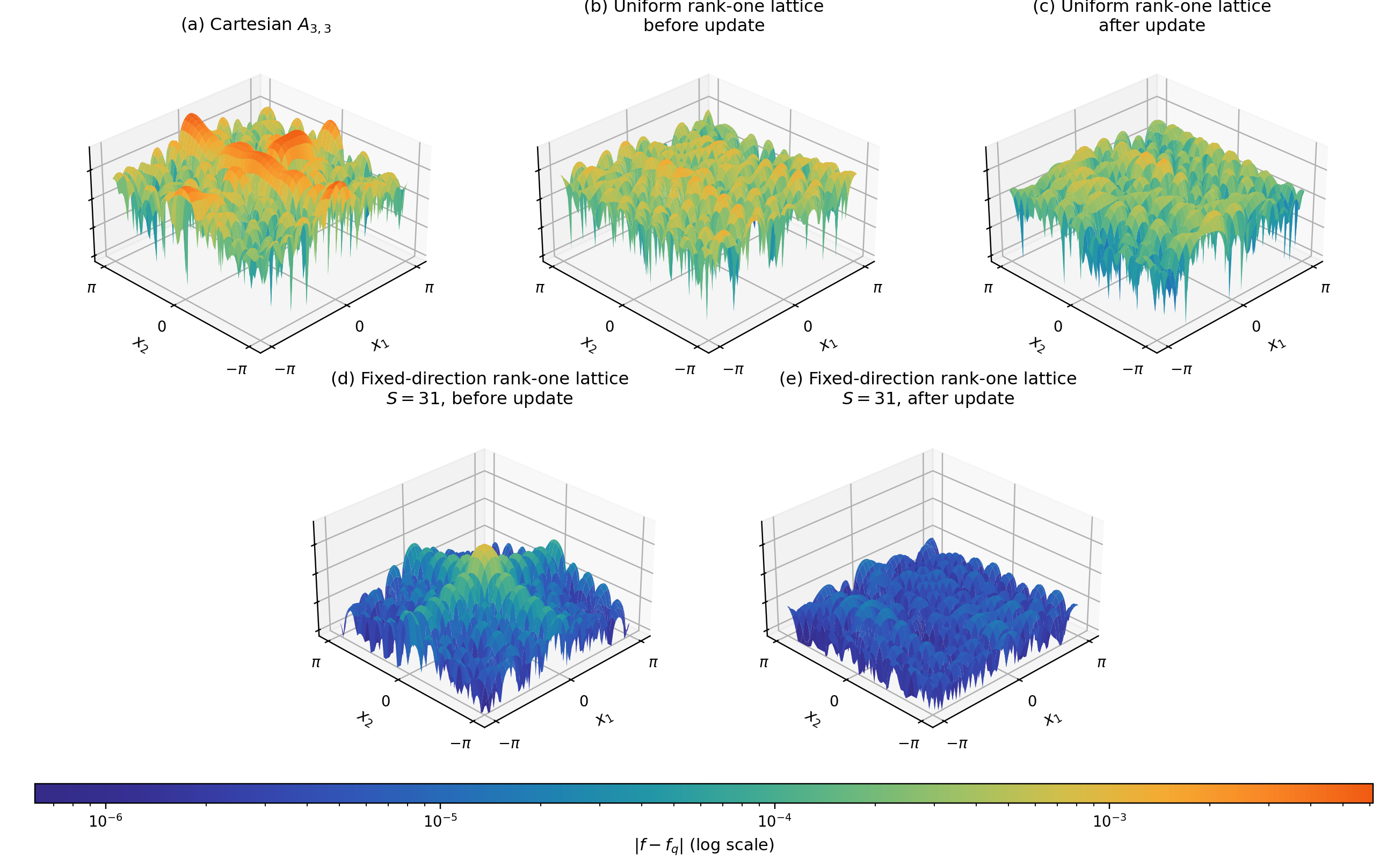
After centering the torus for visualization, one can see in Figure 3 that produces two pronounced ridges along the row and column where its recursions are initialized. Instead, the error of the updated rank-one lattices is distributed without a preferred row or column. However, before the update, the quantized rank-one values, in both the uniform and fixed direction lattices, produce an error near the closing point of the trajectory, compatible with the fact that the initial boundary term has not been eliminated. Observe that, as expected from theory, the approximation via the fixed direction rank-one lattice yields smaller reconstruction errors.

6.2 Comparison on a single function
We next consider one nonconstant function from the same bandlimited test family. Figure 5 shows the pointwise absolute reconstruction errors in log scale and for the different schemes. The Cartesian reconstruction retains the axis-aligned cross, whereas neither spiral reconstruction exhibits ridges extending across the torus. Overall, the error for the rank-one lattice schemes, the constant update reduces the reconstruction error of the updated signals. In particular, for the rank-one lattice with fixed direction, the boundary artifact in the origin is eliminated in the updated scheme.

6.3 An example of a halftoned periodic image
We consider the Shepp–Logan phantom, which is a periodic image, and we scale its gray values (in ) such that after it is mapped to by , the resulting range is contained in so that no instability can arise due to large signal amplitude. The high-resolution periodic image is treated as a continuous input through periodic bilinear interpolation, applying a preliminary low-pass filter. We take and reconstruct the image using three different methods. The Cartesian experiment uses the weighted scheme from [5], i.e., the filter is applied on both the vertical and horizontal direction with both weights and initialization. The same filter is also used for both the rank-one experiments. Moreover, the uniform rank-one lattice has points and a generator , while the fixed-direction lattice has points and generator , with . These choices satisfy the stability condition for the second-order quantizers used here.
For display only, only the halftoned images are translated periodically by , so that the origin and the two torus seams appear at the center. This translation changes neither the bit sequences nor the reconstructions.
In the rank-one panels, each bit is instead extended over its exact fundamental rectangle and the cells are rasterized at resolution , rather than assigned to the nearest Cartesian pixel. Figure 6 shows that all the discretizations lead to good halftoned images; however, for the scheme , one indeed observes line artifacts along the horizontal and vertical initialization boundaries. As expected, for the uniform rank-one scheme, this effect is no longer visible, but the general appearance is slightly coarser. For the fixed direction rank-one lattice with rectangular pixels, not only are the boundary effects removed, but also the shading of the grey areas looks more uniform.


7 Conclusions and outlook
In this work, we studied the boundary mismatch produced by Sigma–Delta schemes on the two-dimensional torus. By arranging the samples along a single closed rank-one lattice, we replaced the multiple boundary contributions arising from separately initialized rows and columns by a single terminal contribution, while preserving exact reconstruction of bandlimited functions. For the uniform lattice, we obtained first- and second-order error bounds of order and , respectively. A suitable global update eliminates the terminal mismatch and reduces the spatial localization of the error. For fixed-direction lattices, compensating for the constant update leads to the improved rates and , at the cost of a less uniform sampling geometry. The numerical experiments support the reduction of boundary artifacts predicted by this construction. A natural direction for future work is to extend this idea to other closed domains and manifolds. The general objective is to identify suitable sampling curves or orderings that allow standard one-dimensional Sigma–Delta schemes to be applied while remaining compatible with the geometry and reconstruction theory of the underlying domain. Further questions include the extension to higher-order Sigma–Delta schemes, the design of schemes for the classical Cartesian sampling, more general stable feedback filters, and broader signal models beyond bandlimited functions.
References
- [1] (2009) Halftone visual cryptography via error diffusion. IEEE transactions on information forensics and security 4 (3), pp. 383–396. Cited by: §1.
- [2] (2000) Modeling and quality assessment of halftoning by error diffusion. IEEE Transactions on image processing 9 (5), pp. 909–922. Cited by: §1.
- [3] (2001) Adaptive threshold modulation for error diffusion halftoning. IEEE Transactions on Image Processing 10 (1), pp. 104–116. Cited by: §1.
- [4] (2025) The mathematics of dots and pixels: on the theoretical foundations of image halftoning. GAMM-Mitteilungen 48 (1), pp. e70000. Cited by: §1.
- [5] (2023) Enhanced digital halftoning via weighted Sigma–Delta modulation. SIAM Journal on Imaging Sciences 16, pp. 1727–1761. Cited by: §1, §1, §1, §2, Figure 1, Figure 1, §3, §6.3, §6.
- [6] (1963) A unity bit coding method by negative feedback. Proceedings of the IEEE 51 (11), pp. 1524–1535. Cited by: §1, §1.
- [7] (1997) Digital halftoning as 2-D delta–sigma modulation. In Proceedings of the IEEE International Conference on Image Processing, Vol. 1, pp. 799–802. Cited by: §1.
- [8] (2003) Approximating a bandlimited function using very coarsely quantized data: a family of stable Sigma–Delta modulators of arbitrary order. Annals of Mathematics 158 (2), pp. 679–710. Cited by: §1, §2, §2.
- [9] (2003) One-bit Sigma–Delta quantization with exponential accuracy. Communications on Pure and Applied Mathematics 56 (11), pp. 1608–1630. Cited by: §1, §2, §2, §4.1.
- [10] (2011) An optimal family of exponentially accurate one-bit Sigma–Delta quantization schemes. Communications on Pure and Applied Mathematics 64 (7), pp. 883–919. Cited by: §1.
- [11] (2023) One-bit Sigma–Delta modulation on the circle. Advances in Computational Mathematics 49, pp. 32. External Links: Document Cited by: §1, §1, §1, §3, §3, §4.1, Remark 4.6, Remark 4.6, Remark 4.6, §5.
- [12] (2008) Sigma–delta quantization errors and the traveling salesman problem. Advances in Computational Mathematics 28 (2), pp. 101–118. Cited by: §1.
- [13] (2007) Frame paths and error bounds for sigma–delta quantization. Applied and Computational Harmonic Analysis 22 (2), pp. 176–197. Cited by: §1.
- [14] (2007) Smooth frame-path termination for higher order sigma-delta quantization. Journal of Fourier Analysis and Applications 13 (3), pp. 285–307. Cited by: §1.
- [15] (1999) Digital halftoning algorithm based on random space-filling curve. IEICE TRANSACTIONS on Fundamentals of Electronics, Communications and Computer Sciences 82 (3), pp. 553–556. Cited by: §1, §1.
- [16] (2006) Second-order sigma–delta () quantization of finite frame expansions. Applied and Computational Harmonic Analysis 20 (1), pp. 126–148. Cited by: §1.
- [17] (2018) One-bit sigma-delta modulation on a closed loop. In 2018 IEEE Statistical Signal Processing Workshop (SSP), pp. 208–212. Cited by: §1.
- [18] (1991) Digital halftoning with space filling curves. ACM SIGGRAPH Computer Graphics 25 (4), pp. 81–90. Cited by: §1.
- [19] (2021) Approximation of high-dimensional periodic functions with fourier-based methods. SIAM Journal on Numerical Analysis 59 (5), pp. 2393–2429. Cited by: §1, §4, §4, §4, §5.
- [20] (2021) Function integration, reconstruction and approximation using rank-1 lattices. Mathematics of Computation 90 (330), pp. 1861–1897. Cited by: §1.
- [21] (2022) Sparse fourier transforms on rank-1 lattices for the rapid and low-memory approximation of functions of many variables. Sampling Theory, Signal Processing, and Data Analysis 20 (1), pp. 1. Cited by: §1.
- [22] (2011) An optimal family of exponentially accurate one-bit sigma-delta quantization schemes. Communications on Pure and Applied Mathematics 64 (7), pp. 883–919. Cited by: §2.
- [23] (2026) On trajectory-based stability analysis for -bit sigma-delta quantization and its application to the second-order case. arXiv preprint arXiv:2605.17127. Cited by: Remark 4.3.