Trajectory Statistics Govern Mechanical Power Transfer in Active Baths

Chul-Ung Woo Email: chul-ung.woo@uni-saarland.de Affiliation: Department of Theoretical Physics and Center for Biophysics, Saarland University, Saarbrücken, Germany Jiwon Choi Email: chlwldnjs175@gmail.com Affiliation: Department of Theoretical Physics and Center for Biophysics, Saarland University, Saarbrücken, Germany Heiko Rieger Email: heiko.rieger@uni-saarland.de Affiliation: Department of Theoretical Physics and Center for Biophysics, Saarland University, Saarbrücken, Germany

September 15, 2026

Abstract

The mechanical response of a moving probe in an active bath reflects both the dynamics of the bath and how the probe couples to it. For a probe moving at velocity $\bm{V}$ and interacting weakly with an ideal active bath, we show that the trajectory statistics of a free bath particle determine a density response from which the bath force on the probe follows. The probe-particle interaction determines how this response is weighted over wave vector $\bm{q}$ , while the probe motion selects frequencies $\omega_{\bm{q}}=\bm{q}\cdot\bm{V}$ . This trajectory-response relation separates the bath dynamics from the wave-vector weighting, so neither the stationary state nor force correlations need to be recalculated for each probe interaction and velocity. Applying this relation to active-particle models, we prove that positive power transfer is excluded for active Ornstein–Uhlenbeck particles in all dimensions and for complete-reset run-and-tumble particles in $d\geq 2$ , while one-dimensional run-and-tumble particles and two-dimensional active Brownian particles possess modes that can transfer positive mechanical power. For a given probe, this response predicts drag reversal, spontaneous probe motion, and motion-induced density distortions, all in quantitative agreement with simulations. Varying the probe geometry changes how the same bath response is weighted, thereby selecting different moving states. Beyond the leading weak-probe, ideal-bath limit, higher orders in probe strength involve multi-interval trajectory statistics, while finite-density corrections involve interacting-particle dynamics. Our results connect the trajectory statistics of active bath particles to the mechanical response of a passive probe, providing a route to predict probe response from single-particle trajectory statistics measured in the absence of the probe.

I Introduction

Passive objects immersed in active media provide a direct probe of nonequilibrium transport and mechanical coupling, and of how microscopic self-propulsion is transferred across scales [22, 105, 100, 9, 40]. Experiments across microbial suspensions, motile-cell carpets, bacterial turbulence, and active granular media have revealed enhanced and non-Gaussian transport, transient superdiffusion, and persistent tracer memory [110, 60, 70, 46, 45, 42, 111, 16]. Theoretical studies have related these effects to steric swimmer–tracer encounters and activity-driven force fluctuations [13, 31], as well as interaction-induced memory in crowded active suspensions [87]. Beyond tracer transport, active media can mediate interactions between passive bodies [72, 5, 39] and drive directed motion of asymmetric objects [2, 97, 33, 65, 83, 79, 74].

For externally driven probe motion, microrheology characterizes the force-velocity response [49, 88, 14, 81, 53, 47]. In active media, a striking nonequilibrium response is negative drag: the bath force has a component in the direction of the probe velocity and transfers positive mechanical power to the probe. Unlike geometric rectification, negative drag can occur for a symmetric object in an inversion-symmetric bath [37, 41, 51]. A forward force contribution does not by itself imply negative total drag, as illustrated by rear accumulation in interacting active Brownian particle (ABP) suspensions [52]. These observations motivate asking how the bath dynamics and probe-particle interaction combine to determine the net force on a moving probe.

Previous approaches have described friction, noise, memory, and driven density profiles for probes in nonequilibrium media [62, 29, 63, 77, 12, 98, 27]. Related coarse-grained active-matter theories characterize effective interactions and responses to external perturbations [103, 26, 48]. In dilute active baths, recent work has obtained velocity-dependent friction and noise for probes in one-dimensional run-and-tumble particle (RTP) and two-dimensional ABP systems [78]. Such probe responses are often expressed through stationary distributions or dynamical correlations of the medium conditioned on the probe configuration or motion [62, 63, 77, 78].

Refer to caption — Figure 1: From free-particle motion to the mechanical response of a moving probe. The moving-probe problem separates into a bath response determined by the free-particle self-ISF, frequency sampling set by the probe velocity, and wave-vector weighting set by the probe-bath interaction. The right panels illustrate the sampled responses for two probe velocities together with the interaction weight. Combining them in the force integral gives the bath force and the mechanical power transferred from the bath to the probe.

For uniformly moving perturbations in other physical systems, the dynamics of the medium and the spatial form of the perturbation enter the force separately [30, 28, 4, 23]. For a perturbation moving with velocity $\bm{V}$ , a Fourier component with wave vector $\bm{q}$ is sampled at the frequency $\bm{q}\cdot\bm{V}$ . The response of ABPs to spatially varying activity has also been related to particle trajectory statistics [96]. The self-intermediate scattering function (self-ISF), the Fourier transform of the displacement distribution, resolves these free-particle statistics in time and wave number [106, 56].

We show that free-particle displacement statistics determine the density and force responses of a uniformly moving probe [Fig. 1]. Section II derives this trajectory-response relation, and Section III uses it to classify mechanical power transfer for the active-particle models considered here. Section IV shows how the wave-vector weighting set by the probe interaction determines the drag and density profile. Section V examines how varying the probe velocity changes the sampled frequencies, while Section VI shows how probe geometry changes the angular weighting and selects the directions of motion. Finally, Section VII extends the trajectory-response framework beyond the leading weak-probe, ideal-bath limit through higher-order single-particle trajectory statistics and a low-density expansion for interacting baths.

II trajectory-response Relation

We consider a dilute ideal gas of noninteracting active particles with far-field number density $\rho_{0}$ . A passive probe is translated at a constant velocity $\bm{V}$ and interacts with each bath particle through a localized real potential $U(\bm{r})$ , where $\bm{r}$ denotes the particle position relative to the probe. Let $\rho(\bm{r};\bm{V})$ be the stationary particle density in the probe frame, with $\rho(\bm{r};\bm{V})\to\rho_{0}$ far from the probe. The force exerted by the bath on the probe is

\bm{F}_{\rm bath}(\bm{V})=\int\mathrm{d}^{d}r\,\rho(\bm{r};\bm{V})\nabla U(\bm{r}).

(1)

Writing

\rho(\bm{r};\bm{V})=\rho_{0}+\delta\rho(\bm{r};\bm{V}),

(2)

the uniform contribution vanishes because $\int\mathrm{d}^{d}r\,\nabla U=0$ . The force depends only on the density perturbation,

\bm{F}_{\rm bath}(\bm{V})=\int\mathrm{d}^{d}r\,\delta\rho(\bm{r};\bm{V})\nabla U(\bm{r}).

(3)

The propulsion is represented by a stationary Markov process with internal state $s_{t}$ , active velocity $\bm{u}(s_{t})$ , stationary distribution $\pi(s)$ , and forward generator $\mathcal{L}_{s}$ . The stationary distribution satisfies $\mathcal{L}_{s}\pi=0$ and $\int\mathrm{d}s\,\pi(s)=1$ . In the probe frame, the relative particle position obeys

\dot{\bm{r}}=\bm{u}(s_{t})-\bm{V}-\mu\nabla U(\bm{r})+\sqrt{2D_{t}}\,\bm{\eta}(t).

(4)

Here $\mu$ is the particle mobility, $D_{t}$ is the translational diffusivity, and $\bm{\eta}$ is a unit Gaussian white noise independent of the propulsion process. Within this class, the active process need not be Gaussian or isotropic.

Let $P(\bm{r},s,t)$ denote the number density resolved with respect to the propulsion state. Its evolution is

	$\displaystyle\partial_{t}P=$	$\displaystyle-\bigl[\bm{u}(s)-\bm{V}\bigr]\cdot\nabla P+D_{t}\nabla^{2}P$		(5)
		$\displaystyle+\mathcal{L}_{s}P+\mu\nabla\cdot\left[P\nabla U\right].$		(5)

For a weak probe potential, we write

P(\bm{r},s,t)=\rho_{0}\pi(s)+\delta P(\bm{r},s,t)+\mathcal{O}(U^{2}).

(6)

Here $\delta P=\mathcal{O}(U)$ , and the density perturbation is $\delta\rho(\bm{r},t)=\int\mathrm{d}s\,\delta P(\bm{r},s,t)$ .

Keeping only terms linear in $U$ gives

\partial_{t}\delta P=\mathcal{L}_{0}\,\delta P+\mu\rho_{0}\pi(s)\nabla^{2}U(\bm{r}).

(7)

Here

\mathcal{L}_{0}=-\bigl[\bm{u}(s)-\bm{V}\bigr]\cdot\nabla+D_{t}\nabla^{2}+\mathcal{L}_{s}

(8)

generates the dynamics of a free bath particle in the moving probe frame. The omitted term $\mu\nabla\cdot[\delta P\nabla U]$ is of $\mathcal{O}(U^{2})$ in the density equation and contributes only at $\mathcal{O}(U^{3})$ to the force.

Note that $e^{t\mathcal{L}_{0}}$ is the free propagator defined by the homogeneous part of Eq. (7) and $\pi\nabla^{2}U$ is the inhomogeneous part. For $\delta P({\bf r},s,0)=0$ , the solution of the linear equation is

\delta P({\bf r},s,t)=\mu\rho_{0}\int_{0}^{t}\mathrm{d}t^{\prime}\,\mathrm{e}^{(t-t^{\prime})\mathcal{L}_{0}}\left[\pi(s)\nabla^{2}U\right].

(9)

The action of this propagator can be represented directly as an average over free-particle trajectories. Their stochastic displacements in the probe frame during a time interval $t$ are given by

\Delta\bm{r}_{t}=\int_{0}^{t}\mathrm{d}t^{\prime}\,\bm{u}(s_{t^{\prime}})-\bm{V}t+\sqrt{2D_{t}}\,\bm{W}_{t},

(10)

where $\bm{W}_{t}$ denotes the standard $d$ -dimensional Wiener process (i.e., the spatial displacement of diffusive trajectories after time $t$ ) and $s_{t^{\prime}}$ denotes stochastic trajectories in the internal state space. For any spatial function $f(\bm{r})$ , translational invariance of the free dynamics gives

\int\mathrm{d}s\,\left[e^{t\mathcal{L}_{0}}(\pi f)\right](\bm{r},s)=\left\langle f\!\left(\bm{r}-\Delta\bm{r}_{t}\right)\right\rangle,

(11)

where $(\pi f)(\bm{r},s)\equiv\pi(s)f(\bm{r})$ , and the average is over free trajectories whose initial propulsion state is drawn from the stationary distribution $\pi(s)$ . Applying Eq. (11) to $f=\nabla^{2}U$ in Eq. (9) and taking the stationary limit ( $t\to\infty$ ) gives the real-space trajectory representation

\delta\rho(\bm{r};\bm{V})=\mu\rho_{0}\int_{0}^{\infty}\mathrm{d}t\,\left\langle\nabla^{2}U\!\left(\bm{r}-\Delta\bm{r}_{t}\right)\right\rangle.

(12)

Thus the stationary density perturbation is obtained by averaging the probe-induced source over free-particle displacements in the moving frame.

To express Eq. (12) in Fourier space, we use the Fourier convention

f(\bm{r})=\int_{\bm{q}}\mathrm{e}^{\mathrm{i}\bm{q}\cdot\bm{r}}f_{\bm{q}},

(13)

where $\int_{\bm{q}}\equiv\int\mathrm{d}^{d}q/(2\pi)^{d}$ . The Fourier-space density response is

\delta\rho_{\bm{q}}(\bm{V})=-\mu\rho_{0}q^{2}U_{\bm{q}}\int_{0}^{\infty}\mathrm{d}t\,\left\langle\mathrm{e}^{-\mathrm{i}\bm{q}\cdot\Delta\bm{r}_{t}}\right\rangle.

(14)

Using the probe-frame displacement in Eq. (10), the trajectory average can be written as

	$\displaystyle\left\langle\mathrm{e}^{-\mathrm{i}\bm{q}\cdot\Delta\bm{r}_{t}}\right\rangle$	$\displaystyle=\mathrm{e}^{\mathrm{i}\omega_{\bm{q}}t}\Phi_{0}(\bm{q},t)$		(15)
		$\displaystyle=\mathrm{e}^{\mathrm{i}\omega_{\bm{q}}t}\mathrm{e}^{-D_{t}q^{2}t}\phi_{\rm a}(\bm{q},t),$		(15)

where $\omega_{\bm{q}}\equiv\bm{q}\cdot\bm{V}$ . With $\Delta\bm{r}_{0,t}\equiv\Delta\bm{r}_{t}+\bm{V}t$ denoting the laboratory-frame displacement,

\Phi_{0}(\bm{q},t)=\left\langle\mathrm{e}^{-i\bm{q}\cdot\Delta\bm{r}_{0,t}}\right\rangle

(16)

is the full free-particle self-intermediate scattering function (ISF), i.e., the spatial Fourier transform of the free-particle displacement distribution [106, 56]. The factor $\phi_{\rm a}(\bm{q},t)$ is the active-displacement ISF,

\phi_{\rm a}(\bm{q},t)=\left\langle\exp\left[-\mathrm{i}\bm{q}\cdot\int_{0}^{t}\mathrm{d}t^{\prime}\,\bm{u}(s_{t^{\prime}})\right]\right\rangle.

(17)

The self-ISF $\Phi_{0}(\bm{q},t)$ encodes the finite-time displacement statistics at each wave vector and is generally not determined by the velocity autocorrelation or long-time diffusivity alone. The frequency-dependent density response is therefore

\mathcal{G}(\bm{q},\omega)=\int_{0}^{\infty}\mathrm{d}t\,\mathrm{e}^{\mathrm{i}\omega t}\Phi_{0}(\bm{q},t).

(18)

When the time integral is not conventionally convergent for $D_{t}=0$ , it is understood with an infinitesimal convergence factor.

To connect with standard response notation, define the retarded density susceptibility through $\delta\rho_{\bm{q}}=-\chi_{\rho U}^{R}U_{\bm{q}}$ . The susceptibility then is

\chi_{\rho U}^{R}(\bm{q},\omega)=\mu\rho_{0}q^{2}\mathcal{G}(\bm{q},\omega).

(19)

In the passive diffusive limit $\bm{u}=0$ , Eq. (19) recovers the corresponding classical field response [30, 28]. For thermal diffusion, $D_{t}=\mu k_{\mathrm{B}}T$ , the free-particle self-ISF is proportional to the equilibrium density correlation, and Eq. (19) reduces to the fluctuation-dissipation relation.

For a real potential, $U_{-\bm{q}}=U_{\bm{q}}^{*}$ . Substituting Eq. (19) into Eq. (3) and using $\Im\mathcal{G}(\bm{q},\omega)=(\mathcal{G}(\bm{q},\omega)-\mathcal{G}^{*}(\bm{q},\omega))/2\mathrm{i}$ and $\mathcal{G}^{*}(\bm{q},\omega)=\mathcal{G}(-\bm{q},-\omega)$ gives

F_{{\rm bath},i}(\bm{V})=-\mu\rho_{0}\int_{\bm{q}}q_{i}q^{2}\left|U_{\bm{q}}\right|^{2}\Im\mathcal{G}(\bm{q},\omega_{\bm{q}}).

(20)

Because $\delta\rho=\mathcal{O}(U)$ , Eq. (20) is the leading nonvanishing bath force, of order $\mathcal{O}(U^{2})$ .

Equations (19) and (20) establish the trajectory-response relation for a uniformly moving probe. Equation (19) has the standard form of a linear density response [54, 67, 6, 26], but in the ideal-bath setting considered here its susceptibility is determined entirely by the free-particle self-ISF $\Phi_{0}(\bm{q},t)$ . The probe–particle interaction sets the wave-vector weighting through $\left|U_{\bm{q}}\right|^{2}$ , and the imposed velocity selects the frequency $\omega_{\bm{q}}=\bm{q}\cdot\bm{V}$ . This factorization parallels drag formulas for uniformly moving perturbations in dissipative classical fields and quantum fluids [30, 28, 4, 23], where the medium dynamics and the spatial form of the perturbation likewise enter separately.

Higher orders in the probe potential remain determined by free-particle trajectories but require successive-displacement correlations beyond the self-ISF and can recover Fourier-phase sensitivity, while bath interactions generate a low-density hierarchy beginning with isolated-pair dynamics. These extensions are developed in Sec. VII.

The remainder of the main text focuses on the leading ideal-bath response. For the inversion-symmetric active baths considered below, the sign of $\Im\mathcal{G}(\bm{q},\omega)/\omega$ provides a probe-independent criterion for mechanical power transfer, which we develop in the next section.

III Classification of Mechanical Power Transfer

A first consequence of the trajectory-response relation is a criterion for the direction of mechanical power transfer. For an inversion-symmetric free process,

\Phi_{0}(-\bm{q},t)=\Phi_{0}(\bm{q},t)=\Phi_{0}(\bm{q},t)^{*}.

(21)

It follows that $\Im\mathcal{G}(\bm{q},\omega)$ is odd in frequency and vanishes at $\omega=0$ . Define

\mathcal{K}(\bm{q},\omega)=\frac{\Im\mathcal{G}(\bm{q},\omega)}{\omega}.

(22)

Its value at $\omega=0$ is defined by continuity. Using Eq. (19),

\mu\rho_{0}q^{2}\mathcal{K}(\bm{q},\omega)=\frac{\Im\chi_{\rho U}^{R}(\bm{q},\omega)}{\omega}.

(23)

Equation (20) can then be written as

\displaystyle\bm{F}_{\rm bath}(\bm{V})=-\mu\rho_{0}\int_{\bm{q}}\bm{q}q^{2}\left|U_{\bm{q}}\right|^{2}\omega_{\bm{q}}\mathcal{K}(\bm{q},\omega_{\bm{q}}).

(24)

The mechanical power transferred from the bath to the probe is

	$\displaystyle\dot{W}_{\rm bath}(\bm{V})$	$\displaystyle=\bm{V}\cdot\bm{F}_{\rm bath}(\bm{V})$		(25)
		$\displaystyle=-\mu\rho_{0}\int_{\bm{q}}q^{2}\left\|U_{\bm{q}}\right\|^{2}\omega_{\bm{q}}^{2}\mathcal{K}(\bm{q},\omega_{\bm{q}}).$		(25)

Every factor in the integrand of Eq. (25) other than $\mathcal{K}$ is nonnegative. Consequently,

\mathcal{K}(\bm{q},\omega)\geq 0

(26)

for all wave vectors and frequencies implies

\dot{W}_{\rm bath}(\bm{V})\leq 0

(27)

for every imposed velocity, at the leading nonvanishing order in the probe potential.

This implication requires neither isotropy nor a particular probe geometry. The probe potential changes how strongly different wave-vector modes contribute, but it cannot change their individual signs when Eq. (26) holds.

The converse does not hold for a particular probe. If $\mathcal{K}(\bm{q},\omega)<0$ in some region, those modes can transfer positive mechanical power to the probe. Whether they reverse the total drag depends on how strongly the probe interaction weights them. The existence of such modes is a property of the free-particle dynamics, whereas the sign of the total drag depends on both the bath and the probe.

We apply this criterion to three standard active-particle models [95] with the same two-point velocity correlations,

\left\langle u_{i}(t)u_{j}(0)\right\rangle=\frac{v_{0}^{2}}{d}\mathrm{e}^{-\left|t\right|/\tau}\delta_{ij}.

(28)

They have the same root-mean-square propulsion speed, persistence time, and long-time active diffusivity $D_{a}=v_{0}^{2}\tau/d$ , consistent with the common long-wavelength description of ABP and RTP dynamics [18]. Previous work has shown that matching two-point statistics does not generally fix response or energetic observables [99, 43, 58]. Here, the relevant model dependence is encoded in the trajectory statistics, as reflected in their distinct self-ISFs [68, 56, 21] and in non-Gaussian displacement statistics of RTPs [64] and ABPs [7, 8].

To isolate the propulsion dynamics, all model-specific calculations below are first performed at $D_{t}=0$ . For the isotropic processes, the free-particle response depends on $\bm{q}$ only through its magnitude $q$ . We denote the response in physical units for model $X\in\{\mathrm{AOUP},\mathrm{RTP},\mathrm{ABP}\}$ by $\mathcal{K}_{d}^{X}(q,\omega;D_{t})$ . We use the dimensionless variables

(z,\Omega)=(qv_{0}\tau,\omega\tau).

(29)

Here $z$ is the wave number scaled by the persistence length $v_{0}\tau$ , while $\Omega$ is the frequency scaled by the persistence time $\tau$ . The corresponding dimensionless response is defined by

\mathcal{K}_{d}^{X}(q,\omega;0)=\tau^{2}K_{d}^{X}(z,\Omega).

(30)

The effect of independent translational diffusion is considered after the model classifications.

III.1 AOUPs: positive power is excluded at all speeds

For an isotropic active Ornstein–Uhlenbeck process [36, 69, 10],

\dot{u}_{i}=-\frac{u_{i}}{\tau}+\sqrt{\frac{2v_{0}^{2}}{d\tau}}\,\xi_{i}(t).

(31)

Here the $\xi_{i}$ are independent unit white noises. The active displacement is Gaussian, giving the active-displacement ISF

\phi_{\rm a}^{\mathrm{AOUP}}(q,t)=\exp[-q^{2}\Sigma_{d}(t)].

(32)

The displacement variance entering this expression is

\Sigma_{d}(t)=\frac{v_{0}^{2}\tau}{d}\left[t-\tau\left(1-\mathrm{e}^{-t/\tau}\right)\right].

(33)

Since

\Sigma_{d}^{\prime}(t)=\frac{v_{0}^{2}\tau}{d}\left(1-\mathrm{e}^{-t/\tau}\right)\geq 0,

(34)

$\phi_{\rm a}^{\mathrm{AOUP}}(q,t)$ is positive and monotonically decreasing for every $q>0$ . For $\Omega>0$ , pairing each positive half-period of $\sin(\Omega t/\tau)$ with the following negative half-period gives a nonnegative contribution because $\phi_{\rm a}(\bm{q},t/\tau)\geq\phi_{\rm a}(\bm{q},t/\tau+\pi/\Omega)$ . It follows that

K_{d}^{\mathrm{AOUP}}(z,\Omega)\geq 0.

(35)

This holds for all $z$ , $\Omega$ , and spatial dimensions. Equation (26) therefore gives

\dot{W}_{\rm bath}^{\mathrm{AOUP}}(\bm{V})\leq 0

(36)

for every imposed velocity and any probe coupled through a weak potential.

III.2 Complete-reset RTPs: dimensional dependence

A complete-reset RTP [104, 68, 71] moves with $\bm{u}(t)=v_{0}\bm{n}(t)$ , where $\bm{n}$ is a unit vector. At rate $\alpha=\tau^{-1}$ , the propulsion direction is replaced by an independent direction drawn uniformly from $S^{d-1}$ . The exact Laplace-transformed ISF is known from the run-and-tumble kinetic equation [68]. Appendix A connects this result to the response defined in Eq. (18) and determines its sign.

In one dimension, a complete reset redraws either velocity direction with equal probability and is equivalent to a telegraph process [3, 64] with direct sign-flip rate $(2\tau)^{-1}$ . For $\Omega>0$ , the response is negative precisely when

z^{2}>1+\Omega^{2}.

(37)

Its continuous $\Omega\to 0$ limit is

K_{1}^{\mathrm{RTP}}(z,0)=\frac{1-z^{2}}{z^{4}},

(38)

which is negative for $z>1$ . One-dimensional RTPs possess modes with negative response, allowing positive mechanical power contributions at nonzero sampled frequency.

Such modes are accessible only for probe speeds below the propulsion speed $v_{0}$ . In one dimension, $|\Omega|=(|V|/v_{0})z$ , and Eq. (37) becomes

\left[1-\left(\frac{V}{v_{0}}\right)^{2}\right]z^{2}>1.

(39)

No mode satisfies this condition for $|V|\geq v_{0}$ . At and above the propulsion speed, the bath cannot transfer positive mechanical power to any weak probe at this order.

The higher-dimensional result is qualitatively different: positive power transfer is excluded for RTPs in $d\geq 2$ . Using the known free-particle ISF, we obtain $\mathcal{G}(\bm{q},\omega)$ and hence $K_{d}^{\mathrm{RTP}}(z,\Omega)$ directly. The resulting response satisfies

K_{d}^{\mathrm{RTP}}(z,\Omega)\geq 0

(40)

for all $z$ and $\Omega$ . Substitution into Eq. (26) excludes positive mechanical power transfer. The one-dimensional process is the exceptional case among complete-reset RTPs.

III.3 ABPs: response from angular dynamics

For an active Brownian particle [89, 93], the propulsion velocity is $\bm{u}(t)=v_{0}\bm{n}(t)$ and the orientation undergoes rotational diffusion,

\partial_{t}P(\bm{n},t)=D_{r}\nabla_{S^{d-1}}^{2}P(\bm{n},t).

(41)

Here $\nabla_{S^{d-1}}^{2}$ denotes the angular part of the $d$ -dimensional Laplacian on the unit sphere. Spectral representations of the free-ABP displacement statistics have previously been developed from this angular dynamics in both two and three dimensions [55, 56].

For an ABP, the matching of Eq. (28) gives

\tau=\frac{1}{(d-1)D_{r}}.

(42)

Using Eq. (18), the dimensionless response is

K_{d}^{\mathrm{ABP}}(z,\Omega)=\frac{1}{\Omega}\int_{0}^{\infty}\mathrm{d}\bar{t}\,\sin(\Omega\bar{t})\phi_{\rm a}^{\mathrm{ABP}}(z,\bar{t}),

(43)

where $\bar{t}=t/\tau$ . This expression applies for nonzero $\Omega$ . Its continuous $\Omega\to 0$ limit is

K_{d}^{\mathrm{ABP}}(z,0)=\int_{0}^{\infty}\mathrm{d}\bar{t}\,\bar{t}\,\phi_{\rm a}^{\mathrm{ABP}}(z,\bar{t}).

(44)

No simple closed form is available, so we evaluate $\phi_{\rm a}^{\mathrm{ABP}}$ by expanding the angular dynamics in hyperspherical harmonics. This gives a tridiagonal angular hierarchy. Appendix B gives the operator, matrix elements, continued-fraction evaluation, and numerical implementation.

III.4 Dimension dependence of the ABP response

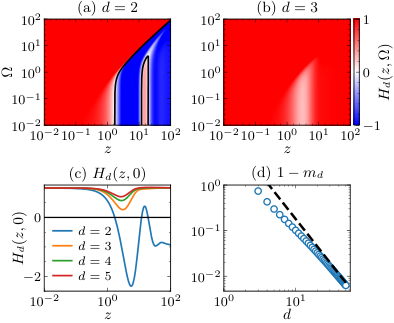
The short-wavelength ABP response is positive at leading order for $d\geq 3$ , but this contribution cancels in $d=2$ , where the first nonzero term is negative. For $z\gg 1$ , the static response is dominated by times $\bar{t}=O(z^{-1})$ , much shorter than the rotational relaxation time [56, 55]. Rotational diffusion is negligible over these times, and we denote by $g_{d}(z\bar{t})$ the characteristic function of its uniform angular distribution. The ABP ISF takes the ballistic form

\phi_{a}^{\mathrm{ABP}}(z,\bar{t})\simeq g_{d}(z\bar{t}).

(45)

With $y=z\bar{t}$ ,

K_{d}^{\mathrm{ABP}}(z,0)\sim\frac{1}{z^{2}}\int_{0}^{\infty}dy\,y\,g_{d}(y).

(46)

This moment equals $d-2$ for $d\geq 3$ , giving

K_{d}^{\mathrm{ABP}}(z,0)=\frac{d-2}{z^{2}}+\mathcal{O}(z^{-3}).

(47)

In $d=2$ , the entire $\mathcal{O}(z^{-2})$ contribution cancels because its coefficient $d-2$ vanishes exactly. The first rotational correction then controls the sign,

K_{2}^{\mathrm{ABP}}(z,0)=-\frac{1}{2z^{3}}+\mathcal{O}(z^{-4}).

(48)

Thus sufficiently short-wavelength modes have negative static response in two dimensions. The finite-frequency response below shows that this negative region extends to nonzero frequencies, where these modes can contribute positive mechanical power.

At long wavelength, by contrast, all dimensions share the same positive asymptotic form,

K_{d}^{\mathrm{ABP}}(z,0)=\frac{d^{2}}{z^{4}}\left[1+\mathcal{O}(z^{2})\right].

(49)

The $z^{-4}$ divergence reflects the diffusive $z^{2}$ relaxation rate of the conserved long-wavelength mode together with the additional factor of time in the static response.

These limiting forms do not exclude a negative region at intermediate wave number or frequency for $d\geq 3$ . To examine the response over the $(z,\Omega)$ plane while removing the asymptotic variation in magnitude, we introduce the rescaled response

H_{d}(z,\Omega)=\left[\Omega^{2}+N_{d}(z)\right]K_{d}^{\mathrm{ABP}}(z,\Omega).

(50)

The normalization function is

N_{d}(z)=\begin{cases}\displaystyle\frac{z^{4}}{d^{2}+(d-2)z^{2}},&d\geq 3,\\[6.0pt] \displaystyle\frac{z^{4}}{4+z/2},&d=2.\end{cases}

(51)

The multiplier in Eq. (50) is strictly positive away from the origin, so $H_{d}$ has the same sign as $K_{d}^{\mathrm{ABP}}$ . For $d\geq 3$ , the normalization removes the known variation in magnitude in the small- $z$ , large- $z$ , and high-frequency limits. For $d=2$ , the large- $z$ static limit is instead $H_{2}(z,0)\to-1$ , preserving the negative tail.

Table 1: Mechanical power classification of the standard propulsion processes in the weak-potential limit. “Positive power excluded” means

\dot{W}_{\rm bath}(\bm{V})\leq 0

for every imposed velocity and every probe coupled through a weak potential.

Process	Dimension	Result	Basis
AOUP	all $d$	positive power excluded	theorem
complete-reset RTP	$d=1$	modes with $K<0$ exist	exact
complete-reset RTP	$d\geq 2$	positive power excluded	theorem
ABP	$d=2$	modes with $K<0$ exist	large- $z$ asymptotics and angular hierarchy
ABP	$d\geq 3$	no mode with $K<0$ found	angular hierarchy at fixed $d$ and large- $d$ asymptotics

In two dimensions, the negative response at $\Omega=0$ extends to nonzero $\Omega$ . For all dimensions $d\geq 3$ considered, $H_{d}$ remains positive throughout the numerically examined domain [Fig. 2]. To quantify its minimum, we define

m_{d}=\min_{z\geq 0,\,\Omega\geq 0}H_{d}(z,\Omega).

(52)

Within numerical accuracy, the minima lie on the $\Omega=0$ boundary and approach $1$ as the dimension increases. The static large- $d$ analysis gives $1-m_{d}=18/d^{2}+\mathcal{O}(d^{-3})$ . The finite-frequency asymptotics also support a minimum at $\Omega=0$ in the large- $d$ limit, consistent with the numerical results. Together with the calculations at fixed $d\geq 3$ , these results support the conjecture

K_{d}^{\mathrm{ABP}}(z,\Omega)\geq 0.

(53)

The derivations of the asymptotic limits, the motivation for the normalization, and the static and finite-frequency large- $d$ analyses are collected in Appendix C.

III.5 Finite-frequency response

Figure 3 compares the finite-frequency responses of the three matched active-particle models in the common dimensionless variables $(z,\Omega)$ . The one-dimensional RTP and two-dimensional ABP contain regions with $K_{d}^{X}<0$ , whereas the AOUP response remains nonnegative.

Linear friction depends only on $K_{d}^{X}(z,0)$ . At nonzero imposed speed, a mode making an angle $\varphi$ with the probe velocity samples the response at $\Omega=(V/v_{0})z\cos\varphi$ . In one dimension, this sampling reduces to $|\Omega|=(|V|/v_{0})z$ . In dimensions $d\geq 2$ , the angular degree of freedom allows $|\Omega|\leq(V/v_{0})z$ at each $z$ . Modes with sufficiently small $|\cos\varphi|$ can sample small frequencies even for $V>v_{0}$ .

III.6 Extension to independent translational diffusion

The preceding classifications were obtained for $D_{t}=0$ . Every result excluding positive power at all speeds remains valid after adding independent translational diffusion of arbitrary strength. Independent translational diffusion changes the self-ISF according to $\Phi_{0}(\bm{q},t)=\mathrm{e}^{-D_{t}q^{2}t}\phi_{\rm a}(\bm{q},t)$ without changing the propulsion statistics.

We write $\mathcal{K}(\bm{q},\omega;D_{t})$ for the response in the presence of translational diffusion. For $D_{t}>0$ and $\bm{q}\neq 0$ ,

$\displaystyle\mathcal{K}(\bm{q},\omega;D_{t})=\frac{4D_{t}q^{2}}{\pi}$	$\displaystyle\int_{0}^{\infty}\mathrm{d}\omega^{\prime}\,\omega^{\prime 2}\mathcal{K}(\bm{q},\omega^{\prime};0)$	(54)
$\displaystyle\times$	$\displaystyle\bigl[(\omega-\omega^{\prime})^{2}+(D_{t}q^{2})^{2}\bigr]^{-1}$
$\displaystyle\times$	$\displaystyle\bigl[(\omega+\omega^{\prime})^{2}+(D_{t}q^{2})^{2}\bigr]^{-1}.$

The kernel in Eq. (54) is nonnegative. Hence,

\mathcal{K}(\bm{q},\omega;0)\geq 0\Longrightarrow\mathcal{K}(\bm{q},\omega;D_{t})\geq 0.

(55)

For each $\bm{q}\neq 0$ , this holds for arbitrary $D_{t}\geq 0$ , with the $D_{t}=0$ case being trivial. The derivation of Eq. (55) is given in Appendix D. Table 1 summarizes which of the standard active-particle models can support positive mechanical power transfer.

IV Interaction Weighting and Drag Reversal

The interaction spectrum $\left|U_{\bm{q}}\right|^{2}$ sets the wave-vector weighting of the bath response characterized in Sec. III. We focus here on the small-velocity regime, beginning with the linear drag.

In the linear limit, only the response at $\Omega=0$ enters,

\mathcal{K}(\bm{q},0)=\int_{0}^{\infty}\mathrm{d}t\,t\,\Phi_{0}(\bm{q},t).

(56)

Writing

F_{{\rm bath},i}(\bm{V})=-\gamma_{ij}V_{j}+\mathcal{O}(V^{2})

(57)

gives

\gamma_{ij}=\mu\rho_{0}\int_{\bm{q}}q_{i}q_{j}q^{2}\left|U_{\bm{q}}\right|^{2}\mathcal{K}(\bm{q},0).

(58)

The corresponding mechanical power at small velocity is

\dot{W}_{\rm bath}(\bm{V})=-\bm{V}^{\mathsf{T}}\frac{\bm{\gamma}+\bm{\gamma}^{\mathsf{T}}}{2}\bm{V}+\mathcal{O}(V^{3}).

(59)

The friction tensor in Eq. (58) is symmetric, so negative linear drag is possible if and only if it has at least one negative eigenvalue.

Having established the extension to finite $D_{t}$ in Sec. III.6, we set $D_{t}=0$ for the remainder of the main text. When comparing different propulsion processes, we use the parameter matching of Eq. (28). The simulation details are given in Appendix J.

IV.1 Linear drag for the standard baths

For the one-dimensional RTP, the wave-number integral can be evaluated for an arbitrary weak potential, recovering the known weak-coupling criterion for symmetric potentials [51]. Substituting Eq. (38) into Eq. (58) and using Parseval’s identity gives

\frac{\gamma_{1}^{\mathrm{RTP}}}{\rho_{0}}=\frac{\mu}{v_{0}^{2}}\int_{-\infty}^{\infty}\mathrm{d}x\,\left[\frac{U(x)^{2}}{(v_{0}\tau)^{2}}-U^{\prime}(x)^{2}\right].

(60)

The linear friction is negative precisely when

(v_{0}\tau)^{2}\frac{\int\mathrm{d}x\,[U^{\prime}(x)]^{2}}{\int\mathrm{d}x\,U(x)^{2}}>1.

(61)

This condition compares the persistence length with a length scale set by the spatial variation of the probe–particle potential.

For the comparison of the different models introduced above, we specialize to the isotropic repulsive Gaussian potential

U_{g}(r)=\epsilon\exp\left(-\frac{r^{2}}{2a^{2}}\right).

(62)

Here $\epsilon>0$ . For a radial probe of characteristic width $a$ , the natural persistence ratio is

\Gamma=\frac{v_{0}\tau}{a}.

(63)

The Fourier transform of the Gaussian potential is

U_{g,\bm{q}}=(2\pi)^{d/2}\epsilon a^{d}\mathrm{e}^{-a^{2}q^{2}/2}.

(64)

Since $\left|U_{g,\bm{q}}\right|^{2}\propto\mathrm{e}^{-a^{2}q^{2}}$ , the corresponding dimensionless radial weight is $\mathrm{e}^{-k^{2}}$ . After the change of variables $k=aq$ , the probe size enters the bath response through $z=k\Gamma$ , while the spatial form of the interaction determines the remaining wave-vector weighting. Writing $G_{d}^{X}(\Gamma)$ for the resulting linear scaling function gives

\frac{\gamma_{d}^{X}}{\rho_{0}}=\frac{\mathcal{A}_{d-1}}{d}\mu\epsilon^{2}\tau^{2}a^{d-4}G_{d}^{X}(\Gamma).

(65)

The scaling function is

G_{d}^{X}(\Gamma)=\int_{0}^{\infty}\mathrm{d}k\,k^{d+3}\mathrm{e}^{-k^{2}}K_{d}^{X}(k\Gamma,0).

(66)

Here $\mathcal{A}_{d-1}$ is the area of $S^{d-1}$ . The corresponding scaling form for a radial potential with a single length scale, including finite $D_{t}$ and arbitrary imposed speed, is given in Appendix E.

For the Gaussian potential, Eq. (60) reduces to

\frac{\gamma_{1}^{\mathrm{RTP}}}{\rho_{0}}=\frac{\sqrt{\pi}\mu\epsilon^{2}}{av_{0}^{2}}\left(\Gamma^{-2}-\frac{1}{2}\right).

(67)

The friction changes sign at $\Gamma_{c,1}^{\mathrm{RTP}}=\sqrt{2}$ : for $\Gamma<\sqrt{2}$ , the positive long-wavelength contribution dominates, whereas for $\Gamma>\sqrt{2}$ the Gaussian interaction gives sufficient weight to modes with $K_{1}^{\mathrm{RTP}}(z,0)<0$ to reverse the total friction.

For the two-dimensional ABP, Eq. (65) becomes

\frac{\gamma_{2}^{\mathrm{ABP}}}{\rho_{0}}=\frac{\pi\mu\epsilon^{2}\tau^{2}}{a^{2}}G_{2}^{\mathrm{ABP}}(\Gamma).

(68)

Numerical evaluation gives a single zero at $\Gamma_{c,2}^{\mathrm{ABP}}\simeq 1.7803$ , with positive friction below and negative friction above. By contrast, $K_{2}^{\mathrm{AOUP}}(z,0)>0$ at every wave number, so the two-dimensional AOUP friction remains positive for all $\Gamma$ .

Figure 4 compares the weak-coupling predictions with direct fixed-velocity particle simulations. The simulations reproduce the transitions of RTPs at $d=1$ and ABPs at $d=2$ , and the positive AOUP friction. The probe is translated at the small but finite speed $V/v_{0}=0.01$ , and the measured force is converted to the friction per bath density according to

\frac{\gamma^{\rm sim}(V)}{\rho_{0}}=-\frac{\left\langle F_{x}(V)\right\rangle}{\rho_{0}V}.

(69)

In the linear regime, $\gamma^{\rm sim}(V)\to\gamma$ as $V\to 0$ .

Figure 4: Linear friction for Gaussian probes in matched ideal active baths. Friction coefficient per bath density,

\gamma/\rho_{0}

, as a function of

\Gamma=v_{0}\tau/a

for (a) a one-dimensional RTP, (b) a two-dimensional ABP, and (c) a two-dimensional AOUP. Solid curves are the

V\to 0

weak-potential predictions obtained by integrating the corresponding responses at

\Omega=0

over wave number with the Gaussian interaction weight. Open circles show direct fixed-velocity simulations at

V/v_{0}=0.01

. Horizontal dashed lines indicate zero friction. The RTP and ABP friction coefficients change sign at

\Gamma_{c,1}^{\mathrm{RTP}}

and

\Gamma_{c,2}^{\mathrm{ABP}}

, respectively, whereas the AOUP friction remains positive.

IV.2 Motion-induced density distortion and force

The drag reversal is accompanied by a reversal of the motion-induced density distortion around the probe. We define $\Delta\rho(\bm{r},V)=\rho(\bm{r},V)-\rho(\bm{r},0)$ . Subtracting the stationary-probe profile removes the inversion-even accumulation generated by the potential and isolates the density change caused by translation.

At leading order in the probe potential, the trajectory-response relation gives

\Delta\rho_{\bm{q}}(V)=-\mu\rho_{0}q^{2}U_{\bm{q}}\left[\mathcal{G}(\bm{q},\omega_{\bm{q}})-\mathcal{G}(\bm{q},0)\right].

(70)

The predicted real-space density difference is obtained by inverse Fourier transformation of Eq. (70).

For an inversion-symmetric bath, $F_{x}(0)=0$ , so the force can be expressed directly in terms of the motion-induced density,

	$\displaystyle F_{x}(V)$	$\displaystyle=\int\mathrm{d}^{2}r\,\Delta\rho(\bm{r},V)\,\partial_{x}U(\bm{r})$		(71)
		$\displaystyle=-\frac{1}{a^{2}}\int\mathrm{d}^{2}r\,xU(\bm{r})\Delta\rho(\bm{r},V).$		(71)

The second equality uses $\partial_{x}U=-xU/a^{2}$ for the Gaussian potential. Only the part of $\Delta\rho(\bm{r},V)$ that is odd under $x\to-x$ contributes to the force, with the local contribution weighted by the probe force.

For the repulsive potential in Eq. (62), an excess of particles in front of the probe, $x>0$ , contributes a force opposite to the direction of motion. An excess behind the probe, $x<0$ , instead contributes a force along the direction of motion.

Density microstructures around driven tracers have previously been studied in passive and active colloidal baths [29, 81, 52]. In interacting two-dimensional ABP suspensions, rear accumulation can generate a forward force contribution without reversing the total drag [52]. The sign of drag depends on the full density distortion weighted by the local probe force in Eq. (71).

Figure 5: Reversal of the motion-induced density distortion in a two-dimensional ABP bath. Normalized motion-induced density,

\Delta\rho(\bm{r},V)/\rho_{0}

V=0.1v_{0}

, around a passive probe moving in the positive

x

direction for (a)

\Gamma=1

and (b)

\Gamma=2.5

. The upper and lower half-planes show particle simulations and the weak-potential theory at finite velocity, respectively, without an independent amplitude fit. At

\Gamma=1

, the density is enhanced in front of the probe and depleted behind it, producing ordinary drag. At

\Gamma=2.5

, the dipolar pattern reverses and the resulting bath force points along the probe velocity. The dashed circle denotes the probe width

a=1

, and the arrow indicates the direction of the imposed velocity.

Figure 5 shows quantitative agreement between the simulations and the weak-potential theory at finite velocity in the spatial form and magnitude of the motion-induced density distortion.

V Velocity Sampling and Spontaneous Probe Motion

The probe velocity selects which frequencies of the bath response are sampled, while the interaction remains fixed. We consider the resulting velocity-dependent force and its nonzero force-balance states for the one-dimensional RTP and two-dimensional ABP, without bare probe friction.

Figure 6: Velocity-dependent force and spontaneous probe motion. (a,b) Effective friction divided by the bath density, for (a) a one-dimensional RTP bath and (b) a two-dimensional ABP bath. Dotted curves are the weak-potential theory at arbitrary speed, and open symbols are fixed-velocity simulations. The representative values of

\Gamma

span regimes of positive linear friction, coexistence of resting and moving states, and negative linear friction; the horizontal line marks

\gamma=0

. (c,d) Positive force-balance roots as functions of

\Gamma

for (c) the one-dimensional RTP and (d) the two-dimensional ABP. Solid and dashed curves denote branches stable and unstable with respect to speed perturbations, respectively, while open circles show long-time speeds from simulations of freely moving probes [see also Supplemental Movie 1 [1]]. Red crosses mark the saddle-node bifurcation points where the stable and unstable moving branches meet. The inset in (d) enlarges the ABP bifurcation region.

V.1 Force balance and high-speed resistance

For an inversion-symmetric isotropic bath and an isotropic probe, the force is parallel to the imposed velocity,

\bm{F}_{\rm bath}(\bm{V})=F_{\parallel}(V)\widehat{\bm{V}}.

(72)

Here $V=\left|\bm{V}\right|>0$ . We define the effective friction by

\gamma(V)=-\frac{F_{\parallel}(V)}{V}.

(73)

This definition applies for $V>0$ , with $\gamma(0)$ defined by continuity. At small speed,

F_{\parallel}(V)=-\gamma(0)V+\mathcal{O}(V^{2}).

(74)

The resting state is linearly stable when $\gamma(0)>0$ and unstable when $\gamma(0)<0$ for the probe dynamics considered below. For $\gamma(0)<0$ , the force points along the motion at sufficiently small positive speed.

At large speed, the force has the asymptotic form

\frac{F_{\parallel}(V)}{\rho_{0}}=-\frac{\mu C_{U}}{V}+o(V^{-1}),

(75)

where $C_{U}=\int_{\bm{q}}q^{2}\left|U_{\bm{q}}\right|^{2}>0$ . The force is asymptotically resistive; this high-speed limit is determined by the short-time passage of bath particles through the probe interaction and is independent of the propulsion process.

For $\gamma(0)<0$ , the opposite signs at small and large speeds guarantee at least one nonzero solution of $F_{\parallel}(V_{*})=0$ by continuity. Assuming that the bath follows the probe velocity quasistatically, the mean radial dynamics gives a stable simple root when $F_{\parallel}^{\prime}(V_{*})<0$ . At a nonzero root, this condition is equivalent to $\gamma^{\prime}(V_{*})>0$ .

Nonzero roots can also occur while $\gamma(0)>0$ . In that case, $\gamma(V)$ must become negative over some intermediate range before returning to its positive high-speed sign. This possibility is realized below for both the RTP and ABP.

V.2 Velocity-dependent force and force-balance branches

We use the persistence ratio $\Gamma$ defined in Eq. (63) and introduce the reduced speed

\nu=\frac{V}{v_{0}}.

(76)

For a Gaussian probe, we write $G_{d}^{X}(\Gamma,\nu)\equiv G_{d}^{X}(\Gamma,\nu,0)$ for the scaling function defined in Appendix E for $D_{t}=0$ . The friction is

\frac{\gamma_{d}^{X}(V)}{\rho_{0}}=\frac{\mathcal{A}_{d-1}}{d}\mu\epsilon^{2}\tau^{2}a^{d-4}G_{d}^{X}(\Gamma,\nu).

(77)

For the one-dimensional RTP process, the force has the nonanalytic small-speed expansion

	$\displaystyle\frac{F_{\parallel}^{\mathrm{RTP}}(V)}{\rho_{0}}=\frac{\mu\epsilon^{2}}{av_{0}}\biggl[$	$\displaystyle-\sqrt{\pi}\left(\Gamma^{-2}-\frac{1}{2}\right)\nu$		(78)
		$\displaystyle+\frac{\pi}{\Gamma^{3}}\nu\left\|\nu\right\|+\mathcal{O}(\nu^{3})\biggr].$		(78)

The linear term reproduces the transition $\Gamma_{c,1}^{\mathrm{RTP}}=\sqrt{2}$ . The $\nu\left|\nu\right|$ term is the one-dimensional form of the nonanalytic correction. In two dimensions, the same long-wavelength contribution gives a $V^{3}\ln(V_{0}/\left|V\right|)$ correction.

For a two-dimensional ABP, the finite-speed response is obtained by evaluating the angular hierarchy at the frequencies $\Omega=\nu z\cos\varphi$ within the Gaussian-probe integral. The resulting force curves and force-balance speeds are obtained numerically and shown in Fig. 6.

The simulations quantitatively reproduce the theoretical effective-friction curves for both the one-dimensional RTP and two-dimensional ABP [Figs. 6(a) and 6(b)]. In both models, stable and unstable moving branches are created at a model-dependent saddle-node $\Gamma_{\rm sn}^{X}<\Gamma_{c}^{X}$ , and the stable branch continues through the linear-instability threshold $\Gamma_{c}^{X}$ [Figs. 6(c) and 6(d)]. For $\Gamma_{\rm sn}^{X}<\Gamma<\Gamma_{c}^{X}$ , a linearly stable resting state coexists with unstable and stable moving states.

At large persistence, the stable force-balance speeds in both systems approach the microscopic propulsion speed $v_{0}$ . The RTP approaches this limit as $\Gamma^{-2}$ , while the ABP shows the slower $\Gamma^{-1/2}$ scaling associated with orientations of small longitudinal relative velocity. The velocity-dependent results are detailed in Appendix F.

A discontinuous symmetry-breaking onset of motion driven by negative drag was previously found for a symmetric penetrable object in a one-dimensional RTP bath [51]. Related reduced probe dynamics in dilute one-dimensional RTP and two-dimensional ABP media describe the transfer of active motion through velocity-dependent friction and noise [78]. Here the stationary force curve obtained from the trajectory–response relation resolves the saddle-node, the coexistence interval, and the stable branch. Within the quasistatic radial dynamics, this branch structure can permit hysteresis under parameter variation and dependence on the initial probe velocity.

VI Geometry Control of Probe Motion

We keep the same isotropic two-dimensional ABP bath and vary only $U$ , changing the wave-vector weighting without changing $\mathcal{K}(q,\omega)$ . Anisotropic passive tracers have previously been used to probe shape-dependent transport in active suspensions [80, 112, 75]. Here we consider two inversion-symmetric geometries: an elliptical Gaussian probe and a probe with fourfold symmetry.

The probe symmetry constrains the force at every imposed velocity. If an orthogonal transformation $\mathcal{R}$ leaves the Fourier-space interaction invariant, $\left|U_{\mathcal{R}\bm{q}}\right|^{2}=\left|U_{\bm{q}}\right|^{2}$ , isotropy of the bath implies

\bm{F}_{\rm bath}(\mathcal{R}\bm{V})=\mathcal{R}\bm{F}_{\rm bath}(\bm{V}).

(79)

At linear order, the friction tensor obeys the same symmetry. Reflection symmetry makes the two body axes of an ellipse principal directions, while fourfold rotational symmetry enforces isotropic linear friction.

Throughout this section, the probe orientation is fixed in the laboratory frame. We consider both the stationary force at imposed velocity and the dynamics of a freely translating probe.

VI.1 Elliptical probe: linear direction selection

As a minimal example of geometry-dependent response, we consider an elliptical Gaussian probe with fixed body axes $\widehat{\bm{e}}_{1}$ and $\widehat{\bm{e}}_{2}$ ,

U_{\rm ell}(x_{1},x_{2})=\epsilon\exp\left(-\frac{x_{1}^{2}}{2a_{1}^{2}}-\frac{x_{2}^{2}}{2a_{2}^{2}}\right),

(80)

where $x_{i}=\bm{r}\cdot\widehat{\bm{e}}_{i}$ and $a_{1}<a_{2}$ . We characterize the probe by the geometric-mean width $a_{g}=\sqrt{a_{1}a_{2}}$ , the aspect ratio $\lambda=a_{2}/a_{1}$ , and the persistence ratio $\Gamma_{g}=v_{0}\tau/a_{g}$ .

Reflection symmetry about the two body axes makes them principal directions of the linear friction, $\bm{\gamma}_{\rm body}=\operatorname{diag}(\gamma_{1},\gamma_{2})$ , while the anisotropic interaction splits the circular-probe threshold into the critical curves $\Gamma_{g,c,1}(\lambda)$ and $\Gamma_{g,c,2}(\lambda)$ . Between them,

\Gamma_{g,c,1}(\lambda)<\Gamma_{g}<\Gamma_{g,c,2}(\lambda),\qquad\gamma_{1}<0<\gamma_{2}.

(81)

Thus the resting state is unstable only along the narrow axis, and this one-axis instability region broadens with increasing aspect ratio [Fig. 7(b)].

The same reflection symmetries make each principal axis an invariant direction of the velocity-dependent force. Along the narrow axis, the force changes from propulsive at small speed to resistive at high speed, producing symmetry-related nonzero force-balance states $\bm{V}=\pm V\widehat{\bm{e}}_{1}$ with stable and unstable branches. Fixed-velocity simulations reproduce the calculated friction along both axes [Fig. 7(c)], while freely translating probes follow the stable narrow-axis branch [Fig. 7(d) and Supplemental Movie 2 [1]].

VI.2 Fourfold probe: nonlinear direction selection and multistability

The fourfold probe is constructed by superposing four copies of the Gaussian potential in Eq. (62), with centers displaced by a distance $b$ from the probe center along the coordinate axes:

U_{4}(\bm{r})=\frac{1}{4}\sum_{\sigma=\pm 1}\left[U_{g}(\bm{r}-\sigma b\widehat{\bm{x}})+U_{g}(\bm{r}-\sigma b\widehat{\bm{y}})\right].

(82)

The normalization ensures that $b=0$ recovers the single Gaussian probe. We use the dimensionless offset $\beta=b/a$ .

For the fourfold interaction, Eq. (79) with $\mathcal{R}=\mathcal{R}_{\pi/2}$ implies fourfold rotational symmetry of the force. Since the linear friction tensor is symmetric, this symmetry forces it to be isotropic. Direction selection can arise only from the nonlinear velocity dependence of the force. Changing $\beta$ switches the selected motion from diagonal to axial, with an intermediate regime of directional multistability [Fig. 8(b)].

We obtain the vector force by substituting the fourfold interaction into the general arbitrary-velocity force in Eq. (20). Uniformly translating states satisfy $\bm{F}_{\rm bath}(\bm{V}_{*})=\bm{0}$ . Unlike the isotropic probe of Sec. V, the force need not be parallel to $\bm{V}$ away from a symmetry direction. Mechanical power transfer depends only on the longitudinal force component, whereas directional selection and stability require the full vector force. Within the quasistatic dynamics generated by the stationary mean force, the stability of a moving root must be determined from the full two-dimensional force Jacobian.

Along the representative cut $\Gamma=6$ , the diagonal moving states are stable at $\beta=2$ , the axial states are stable at $\beta=3$ , and both sets coexist at $\beta=2.5$ [Figs. 8(c)–(e)]. In the multistable regime, four diagonal and four axial attractors are separated by eight oblique saddles.

Freely translating probes reproduce the diagonal, multistable, and axial regimes predicted by the stationary force [Figs. 8(f)–(h) and Supplemental Movies 3–5 [1]]. At $\beta=2.5$ , probes initialized near diagonal and axial attractors remain in distinct long-lived moving states, providing a direct dynamical signature of the predicted directional multistability.

For the ellipse, anisotropic linear friction selects the direction already at small velocity, whereas fourfold symmetry leaves the resting-state instability directionally degenerate and shifts directional selection to the nonlinear velocity dependence of the force. Both potentials are inversion symmetric, so geometry control produces symmetry-related moving states rather than rectification toward a preferred polarity [73, 83, 59, 76]. The response integrals and stability calculations for both probe geometries are given in Appendix G.

VII Extensions of the Trajectory-Response Relation

The leading force derived above is of order $\rho_{0}U^{2}$ . Probe strength and bath density provide two directions in which to extend this result. Introducing a bookkeeping parameter $\lambda_{U}$ through $U\to\lambda_{U}U$ , we organize the force at fixed imposed velocity as the formal double expansion

\bm{F}_{\rm bath}[\lambda_{U}U;\rho_{0}]=\sum_{k=1}^{\infty}\sum_{n=1}^{\infty}\rho_{0}^{k}\lambda_{U}^{n+1}\bm{F}_{\rm bath}^{[k,n]}[U].

(83)

Here $k$ labels the density order and $n$ the order of the probe-induced density perturbation; the force contains one additional factor of $U$ . The coefficients $\bm{F}_{\rm bath}^{[k,n]}$ do not include the displayed factors of $\rho_{0}$ or $\lambda_{U}$ , and their dependence on $\bm{V}$ is implicit. The leading result of Sec. II is the $(k,n)=(1,1)$ term.

Section VII.1 keeps $k=1$ and constructs the higher probe orders from multi-interval single-particle trajectory statistics. Section VII.2 keeps $n=1$ and develops the density expansion, representing the $k=2$ coefficient in terms of isolated-pair dynamics and placing it within the general low-density hierarchy. Mixed coefficients with both $k>1$ and $n>1$ are not evaluated here. Details of the derivations are given in Appendices H and I.

VII.1 Higher orders in the probe potential

Beyond leading order, the self-ISF alone is generally insufficient to determine the probe response; the response depends on multi-time statistics of successive displacement intervals. These higher-order terms fierst introduce sensitivity to probe polarity at $\mathcal{O}(U^{3})$ .

We continue the weak-potential expansion of Eq. (6) by writing

P(\bm{r},s,t)=\rho_{0}\pi(s)+\sum_{n=1}^{\infty}\delta P_{n}(\bm{r},s,t).

(84)

Here $\delta P_{n}=\mathcal{O}(U^{n})$ and $\delta P_{1}\equiv\delta P$ . For $n\geq 2$ , collecting equal powers of $U$ in Eq. (5) gives

\partial_{t}\delta P_{n}=\mathcal{L}_{0}\delta P_{n}+\mu\nabla\cdot\left[\delta P_{n-1}\nabla U\right].

(85)

Repeated application of Eq. (85) introduces consecutive free-propagation intervals of durations $t_{1},\ldots,t_{n}$ . Let $T_{j}=\sum_{\ell=1}^{j}t_{\ell}$ , with $T_{0}=0$ . In Fourier space, let $\bm{q}_{j}$ be the wave vector supplied by the $j$ th probe interaction and define $\bm{Q}_{j}=\sum_{a=1}^{j}\bm{q}_{a}$ . The $j$ th free-propagation interval therefore carries the cumulative wave vector $\bm{Q}_{j}$ , whose mode is sampled by uniform probe motion at $\omega_{\bm{Q}_{j}}$ .

Writing $\delta\rho_{n}(\bm{r})=\int\mathrm{d}s\,\delta P_{n}(\bm{r},s)$ , integration over the final propulsion state then gives

\delta\rho_{n,\bm{q}}=(-\mu)^{n}\rho_{0}\int_{\bm{q}_{1}}\cdots\int_{\bm{q}_{n}}(2\pi)^{d}\delta^{(d)}(\bm{q}-\bm{Q}_{n})\,q_{1}^{2}U_{\bm{q}_{1}}\prod_{j=2}^{n}\left[(\bm{Q}_{j}\cdot\bm{q}_{j})U_{\bm{q}_{j}}\right]\mathcal{G}^{(n)}(\bm{Q}_{1},\ldots,\bm{Q}_{n};\omega_{\bm{Q}_{1}},\ldots,\omega_{\bm{Q}_{n}}),

(86)

where the multi-frequency density response function and the corresponding multi-time generalization of the self-ISF are defined by

	$\displaystyle\mathcal{G}^{(n)}(\bm{Q}_{1},\ldots,\bm{Q}_{n};\omega_{1},\ldots,\omega_{n})={}$	$\displaystyle\int_{0}^{\infty}\mathrm{d}t_{1}\cdots\int_{0}^{\infty}\mathrm{d}t_{n}\,e^{\mathrm{i}\sum_{j=1}^{n}\omega_{j}t_{j}}\Phi_{0}^{(n)}(\bm{Q}_{1},\ldots,\bm{Q}_{n};t_{1},\ldots,t_{n}),$		(87)
	$\displaystyle\Phi_{0}^{(n)}(\bm{Q}_{1},\ldots,\bm{Q}_{n};t_{1},\ldots,t_{n})={}$	$\displaystyle\left\langle\exp\left[-\mathrm{i}\sum_{j=1}^{n}\bm{Q}_{j}\cdot\left(\Delta\bm{r}_{0,T_{j}}-\Delta\bm{r}_{0,T_{j-1}}\right)\right]\right\rangle.$		(88)

The average is over a single free trajectory initialized from $\pi(s)$ , with the propulsion state evolving continuously across the intervals, so the successive displacement increments are generally correlated.

The corresponding contribution to the bath force follows from Eq. (3),

F_{{\rm bath},i}^{(n+1)}=-\mathrm{i}\int_{\bm{q}}q_{i}U_{-\bm{q}}\,\delta\rho_{n,\bm{q}}.

(89)

For $n=1$ , $\mathcal{G}^{(1)}$ reduces to $\mathcal{G}$ , and Eqs. (86) and (89) recover the leading density and force responses of Sec. II. For $n=2$ , related multi-time extensions of the self-ISF have been used to characterize correlations between successive particle displacements in supercooled liquids [50]. Higher-order position and velocity correlations have also been calculated for active Brownian trajectories [102].

At $\mathcal{O}(U^{2})$ , wave-vector conservation gives $U_{\bm{q}}U_{-\bm{q}}=|U_{\bm{q}}|^{2}$ , leaving the leading force insensitive to the Fourier phase and to polarity reversal, $U(\bm{r})\to U(-\bm{r})$ . The cubic correction contains products of the form $U_{\bm{q}}U_{\bm{q}^{\prime}}U_{-\bm{q}-\bm{q}^{\prime}}$ . Unlike $|U_{\bm{q}}|^{2}$ , these products retain information that can distinguish $U(\bm{r})$ from $U(-\bm{r})$ .

VII.2 Finite-density extension to interacting baths

We next include interactions between bath particles while retaining the density response linear in the probe potential. The response form of Eq. (19) for the ideal bath generalizes to

\delta\rho_{\bm{q}}=-\chi_{\rho U}^{R}(\bm{q},\omega_{\bm{q}};\rho_{0})U_{\bm{q}},

(90)

where the susceptibility now contains the density dependence generated by bath-particle interactions. We organize it as $\chi_{\rho U}^{R}(\bm{q},\omega;\rho_{0})=\sum_{k\geq 1}\rho_{0}^{k}\chi^{[k]}(\bm{q},\omega)$ . The leading coefficient is the ideal-bath result, $\chi^{[1]}(\bm{q},\omega)=\mu q^{2}\mathcal{G}(\bm{q},\omega)$ , while the higher-density coefficients describe interaction corrections. Below we show how the first of these corrections is represented in terms of the interacting $N$ -particle dynamics.

We consider translationally invariant pair interactions in the low-density regime and a homogeneous reference state whose one-particle internal distribution is $\pi(s)$ . For $N$ identical bath particles, the probe-frame dynamics of Sec. II generalizes to

	$\displaystyle\dot{\bm{r}}_{a}={}$	$\displaystyle\bm{u}(s_{a})-\bm{V}-\mu\nabla_{a}U(\bm{r}_{a})$		(91)
		$\displaystyle-\mu\sum_{b\neq a}\nabla_{a}W_{ab}+\sqrt{2D_{t}}\,\bm{\eta}_{a}(t).$		(91)

Here $W_{ab}=W(\bm{r}_{a}-\bm{r}_{b})$ is the positional interaction between bath particles. The internal state $s_{a}$ evolves under the free generator $\mathcal{L}_{s_{a}}$ , and we also allow pair interactions in the internal-state dynamics through a probability-conserving contribution $\mathcal{A}_{a\leftarrow b}$ . Both interactions are translationally invariant.

We use $a\equiv(\bm{r}_{a},s_{a})$ and $da\equiv\mathrm{d}^{d}r_{a}\,\mathrm{d}s_{a}$ to denote a particle state and its integration measure. Let $\Psi_{N}(1,\ldots,N,t)$ be the joint probability density, normalized by $\int d1\cdots dN\,\Psi_{N}=1$ and symmetric under exchange of particle labels. Including both positional and internal-state interactions, its evolution is

	$\displaystyle\partial_{t}\Psi_{N}={}$	$\displaystyle\sum_{a=1}^{N}\left[-\bigl(\bm{u}(s_{a})-\bm{V}\bigr)\cdot\nabla_{a}+D_{t}\nabla_{a}^{2}+\mathcal{L}_{s_{a}}\right]\Psi_{N}+\mu\sum_{a=1}^{N}\nabla_{a}\cdot\left[\Psi_{N}\nabla_{a}U(\bm{r}_{a})\right]$		(92)
		$\displaystyle+\mu\sum_{a=1}^{N}\sum_{b\neq a}\nabla_{a}\cdot\left[\Psi_{N}\nabla_{a}W_{ab}\right]+\sum_{a=1}^{N}\sum_{b\neq a}\mathcal{A}_{a\leftarrow b}\Psi_{N}.$		(92)

For a weak probe, write $\Psi_{N}=\Psi_{N}^{(0)}+\delta\Psi_{N}+\mathcal{O}(U^{2})$ , where $\delta\Psi_{N}=\mathcal{O}(U)$ and $\Psi_{N}^{(0)}$ is the stationary distribution without the probe. This reference state includes the bath interactions and need not factorize. Let $\mathcal{L}_{N}(\bm{V})$ denote the generator in Eq. (92) with the probe term omitted, and write $\mathcal{U}_{a}f=\mu\nabla_{a}\cdot[f\nabla_{a}U(\bm{r}_{a})]$ for the probe contribution acting on a joint density $f$ . Homogeneity makes the reference state stationary also in the moving frame, $\mathcal{L}_{N}(\bm{V})\Psi_{N}^{(0)}=0$ . Keeping terms linear in $U$ gives

\partial_{t}\delta\Psi_{N}=\mathcal{L}_{N}(\bm{V})\delta\Psi_{N}+\sum_{a=1}^{N}\mathcal{U}_{a}\Psi_{N}^{(0)}.

(93)

The source is the action of the probe on the unperturbed interacting bath; its subsequent propagation includes all bath interactions.

Since the bath interactions are translationally invariant, the probe-free generator satisfies

\mathcal{L}_{N}(\bm{V})=\mathcal{L}_{N}(\mathbf{0})+\bm{V}\cdot\sum_{a=1}^{N}\nabla_{a}.

(94)

A Fourier component $U_{\bm{q}}$ generates a source with total wave vector $\bm{q}$ , which is preserved by the probe-free dynamics. The common drift in Eq. (94) therefore contributes only the phase $e^{\mathrm{i}\omega_{\bm{q}}t}$ . Projection onto reduced densities preserves the same total wave vector. Thus, at linear order in $U$ , different Fourier modes do not mix and the imposed velocity enters the density response only through $\omega_{\bm{q}}$ .

The bath force depends only on the one-particle density, so we first reduce the $N$ -particle distribution to its one-particle marginal. We define $f_{1}(1)=N\int d2\cdots dN\,\Psi_{N}$ , which is the interacting-bath counterpart of $P(\bm{r},s,t)$ in Sec. II. Accordingly, $\rho(\bm{r}_{1})=\int\mathrm{d}s_{1}\,f_{1}(1)$ is the spatial density entering Eq. (3). The interaction contribution acting on particle $1$ gives

		$\displaystyle N\mu\sum_{b=2}^{N}\int d2\cdots dN\,\nabla_{1}\cdot\left[\Psi_{N}\nabla_{1}W_{1b}\right]$		(95)
		$\displaystyle=\mu\nabla_{1}\cdot\int d2\,f_{2}(1,2)\nabla_{1}W_{12},$		(95)

where $f_{2}(1,2)=N(N-1)\int d3\cdots dN\,\Psi_{N}$ counts ordered pairs of distinct particles. Exchange symmetry makes the $N-1$ terms on the left identical; this factor is included in $f_{2}$ . Thus the interaction force on particle $1$ depends on the joint state of two particles and cannot in general be determined from $f_{1}$ alone.

We write $\mathcal{L}_{0,a}(\bm{V})$ for the free generator of Eq. (8) acting on particle $a$ . The directed interaction contribution is $\mathcal{I}_{a\leftarrow b}f=\mu\nabla_{a}\cdot[f\nabla_{a}W_{ab}]+\mathcal{A}_{a\leftarrow b}f$ . Including both types of interaction, the one-particle equation is

\partial_{t}f_{1}=\left[\mathcal{L}_{0,1}(\bm{V})+\mathcal{U}_{1}\right]f_{1}+\int d2\,\mathcal{I}_{1\leftarrow 2}f_{2}.

(96)

Retaining two particles instead gives

	$\displaystyle\partial_{t}f_{2}={}$	$\displaystyle\left[\mathcal{L}_{2}(\bm{V})+\mathcal{U}_{1}+\mathcal{U}_{2}\right]f_{2}$		(97)
		$\displaystyle+\int d3\,\left(\mathcal{I}_{1\leftarrow 3}+\mathcal{I}_{2\leftarrow 3}\right)f_{3}.$		(97)

Here $f_{3}(1,2,3)=N(N-1)(N-2)\int d4\cdots dN\,\Psi_{N}$ is the three-particle number density. The isolated-pair generator is $\mathcal{L}_{2}=\mathcal{L}_{0,1}+\mathcal{L}_{0,2}+\mathcal{I}_{12}$ , with $\mathcal{I}_{ab}\equiv\mathcal{I}_{a\leftarrow b}+\mathcal{I}_{b\leftarrow a}$ and the common velocity argument suppressed in this definition. It contains the mutual interaction of particles $1$ and $2$ ; the integral in Eq. (97) accounts for their interactions with a third particle.

Continuing this reduction gives the Bogoliubov–Born–Green–Kirkwood–Yvon (BBGKY) hierarchy [101, 25]. In general, $f_{m}(1,\ldots,m)=\frac{N!}{(N-m)!}\int d(m+1)\cdots dN\,\Psi_{N}$ is the reduced number density of $m$ distinct particles. The generator $\mathcal{L}_{m}(\bm{V})=\sum_{a=1}^{m}\mathcal{L}_{0,a}(\bm{V})+\sum_{1\leq a<b\leq m}\mathcal{I}_{ab}$ includes their free dynamics and all mutual interactions, but excludes the probe and particles outside this set. The hierarchy is

	$\displaystyle\partial_{t}f_{m}={}$	$\displaystyle\left[\mathcal{L}_{m}(\bm{V})+\sum_{a=1}^{m}\mathcal{U}_{a}\right]f_{m}$		(98)
		$\displaystyle+\sum_{a=1}^{m}\int d(m+1)\,\mathcal{I}_{a\leftarrow m+1}f_{m+1}.$		(98)

Each equation therefore requires the joint density of one additional particle.

At low density, $f_{m}$ starts at order $\rho_{0}^{m}$ for fixed retained coordinates. Let $f_{m}^{(0)}$ be the corresponding marginal of $\Psi_{N}^{(0)}$ and write $f_{m}=f_{m}^{(0)}+\delta f_{m}+\mathcal{O}(U^{2})$ . The linear probe response can be organized as

\delta f_{m}=\sum_{k=m}^{\infty}\rho_{0}^{k}\delta f_{m}^{[k]}.

(99)

Here $\delta f_{m}^{[k]}$ is linear in $U$ and does not include the displayed factor $\rho_{0}^{k}$ . At order $\rho_{0}U$ , the reference density $f_{1}^{(0)}(1)=\rho_{0}\pi(s_{1})$ gives the ideal-bath response of Sec. II. At order $\rho_{0}^{2}U$ , terms involving $f_{3}$ do not contribute, so the first interaction correction can be expressed entirely in terms of the one- and two-particle equations. This density truncation does not assume weak pair interactions: repeated interactions within the same pair remain included in $\mathcal{L}_{2}$ . The required reference pair density is $f_{2}^{(0)}(1,2)=\rho_{0}^{2}g_{2}(1,2)+\mathcal{O}(\rho_{0}^{3})$ , where $g_{2}$ is the leading stationary pair distribution and approaches $\pi(s_{1})\pi(s_{2})$ as $|\bm{r}_{1}-\bm{r}_{2}|\to\infty$ [85, 32].

For the stationary response, define $\delta\rho_{\bm{q}}^{[k]}=\int d1\,e^{-\mathrm{i}\bm{q}\cdot\bm{r}_{1}}\delta f_{1}^{[k]}(1)$ , so that $\delta\rho_{\bm{q}}=\sum_{k\geq 1}\rho_{0}^{k}\delta\rho_{\bm{q}}^{[k]}$ . Using the wave-vector conservation and frequency sampling established above, the pair-order density coefficient can be written as

	$\displaystyle\delta\rho_{\bm{q}}^{[2]}={}$	$\displaystyle U_{\bm{q}}\int_{0}^{\infty}\mathrm{d}t_{1}\int_{0}^{\infty}\mathrm{d}t_{2}$		(100)
		$\displaystyle\times e^{\mathrm{i}\omega_{\bm{q}}(t_{1}+t_{2})}\mathcal{C}_{2}(\bm{q};t_{1},t_{2}).$		(100)

The kernel $\mathcal{C}_{2}$ collects the pair-order dynamics contributing to the one-particle density: the probe-induced pair response propagates for a time $t_{2}$ , is transferred to the one-particle sector through the pair interaction, and then propagates for a further time $t_{1}$ . Comparison with the susceptibility expansion introduced above gives $\delta\rho_{\bm{q}}^{[2]}=-\chi^{[2]}(\bm{q},\omega_{\bm{q}})U_{\bm{q}}$ , so that $\rho_{0}^{2}\chi^{[2]}$ is the first interaction correction to the density susceptibility.

As a simple limit, set $\mathcal{A}_{a\leftarrow b}=0$ and take a weak positional pair potential, with $W(\bm{r})=\int_{\bm{q}}e^{\mathrm{i}\bm{q}\cdot\bm{r}}W_{\bm{q}}$ . To first order in $W$ , the two propagation intervals contribute the free-particle self-ISFs,

\displaystyle\mathcal{C}_{2}(\bm{q};t_{1},t_{2})=\mu^{2}q^{4}W_{\bm{q}}\Phi_{0}(\bm{q},t_{1})\Phi_{0}(\bm{q},t_{2})+\mathcal{O}(W^{2}).

(101)

Using the time transform in Eq. (18) gives

\chi^{[2]}(\bm{q},\omega)=-\mu^{2}q^{4}W_{\bm{q}}\mathcal{G}(\bm{q},\omega)^{2}+\mathcal{O}(W^{2}).

(102)

The two factors of $\mathcal{G}$ come from the two propagation intervals, while $W_{\bm{q}}$ couples the responses of the two particles.

Returning to the force, keeping the leading probe-potential order while retaining the density dependence of the susceptibility gives

F_{{\rm bath},i}(\bm{V})=-\int_{\bm{q}}q_{i}|U_{\bm{q}}|^{2}\Im\chi_{\rho U}^{R}(\bm{q},\omega_{\bm{q}};\rho_{0})+\mathcal{O}(U^{3}).

(103)

Bath interactions enter through the higher-density coefficients of $\chi_{\rho U}^{R}$ , beginning with the contribution $\rho_{0}^{2}\chi^{[2]}$ . Thus, at this order, interactions modify the bath susceptibility while the probe weighting $|U_{\bm{q}}|^{2}$ and the frequency sampling $\omega_{\bm{q}}$ retain the same structure as in the ideal bath.

VIII Conclusion and Discussion

We have developed a weak-coupling theory in which the self-ISF determines the leading density and mechanical responses of a moving conservative probe in a dilute ideal active bath. This structure can be summarized schematically as

	$\displaystyle\Phi_{0}(\bm{q},t)\longrightarrow G(\bm{q},\omega)$	$\displaystyle\longrightarrow\mathcal{K}(\bm{q},\omega),$		(104)
	$\displaystyle\{\mathcal{K}(\bm{q},\bm{q}\cdot\bm{V}),\|U_{\bm{q}}\|^{2}\}$	$\displaystyle\longrightarrow\bm{F}_{\rm bath}(\bm{V}).$		(104)

We refer to the first relation connecting the intermediate scattering function, ISF, reflecting the trajectory statistics, with the density response function, as the trajectory-response relation. The second relation then connects the density response together with the probe potential with the force exerted by the bath upon the probe.

The sign of $\mathcal{K}$ provides a probe-independent criterion for mechanical power transfer: $\mathcal{K}\geq 0$ everywhere excludes positive steady power for any weak probe, while regions with $\mathcal{K}<0$ contain modes that can contribute positive power. AOUPs, complete-reset RTPs, and ABPs have different $\mathcal{K}$ even with matched two-point velocity correlations because their trajectory statistics differ. For a given probe, $|U_{\bm{q}}|^{2}$ weights these modes, predicting drag reversal, density distortion, and nonzero force-balance roots in agreement with simulations. Probe geometry can change the mode weighting to stabilize different directions of motion.

The main force and power-transfer results that we derived are valid for leading order $\mathcal{O}(\rho_{0}U^{2})$ in the dilute limit. We extended this framework perturbatively in both probe strength and bath density, through higher-order single-particle trajectory statistics and correlated bath clusters. These expansions do not describe strongly coupled or dense regimes with nonlinear density structure and collective dynamics [86, 66, 14, 81, 39, 40, 37, 11]. Transient or oscillatory probe motion, beyond the steady uniform translation considered here, can additionally depend on bath relaxation and memory [52].

Within the dilute regime, the trajectory-response relation extends to other propulsion processes whenever their free-particle displacement statistics can be determined [56, 92, 113, 57, 91, 94, 90]. The same weak-coupling approach could be extended to combined translation and rotation, including probes in dilute chiral baths [61, 84, 44]: for an orientable probe with interaction $U(\bm{r},\theta)$ , the conjugate derivative $-\partial_{\theta}U$ gives the bath torque.

The moving probe considered here could be implemented experimentally as a localized, translating optical potential that forms a penetrable energy landscape for colloidal and active particles [35, 15]. Free-particle displacement statistics can be measured independently by single-particle tracking or ISF techniques such as differential dynamic microscopy [19, 108, 55, 113, 57]. These measurements could be used to determine $\mathcal{K}(q,\omega)$ and predict the leading force for weak probes with different shapes and imposed velocities. The same relation can be used in reverse: measurements obtained while varying the probe size, shape, and velocity can constrain the wave-vector and frequency dependence of $\mathcal{K}(q,\omega)$ . Taken together, our results establish an experimentally accessible connection between free-particle trajectory statistics and the mechanical response of a passive probe, two complementary routes to the same bath response.

Acknowledgements.

We thank Jae Dong Noh for helpful discussions.

Data Availability

The code used for the numerical evaluation of the theory presented in this work will be made publicly available upon publication.

Appendix A Complete-reset RTP response

The complete-reset RTP considered here coincides with the ideal run-and-tumble process analyzed in [68]. Choose the polar axis along $\bm{q}$ and write $x=\bm{n}\cdot\widehat{\bm{q}}$ . Define the orientationally averaged single-run transform

\widetilde{g}_{d}(q,s)=\left\langle\frac{1}{s+\mathrm{i}qv_{0}x}\right\rangle_{\bm{n}}.

(105)

Here $\Re s>0$ and the average is over a uniformly distributed orientation. The exact single-run results are

\widetilde{g}_{d}(q,s)=\begin{cases}\displaystyle\frac{s}{s^{2}+q^{2}v_{0}^{2}},&d=1,\\[8.61108pt] \displaystyle\left(s^{2}+q^{2}v_{0}^{2}\right)^{-1/2},&d=2.\end{cases}

(106)

With $\sigma$ denoting the Laplace variable of the full RTP active-displacement ISF, the renewal form is

\widetilde{\phi}_{\rm a}^{\mathrm{RTP}}(q,\sigma)=\frac{\widetilde{g}_{d}(q,\sigma+\alpha)}{1-\alpha\widetilde{g}_{d}(q,\sigma+\alpha)}.

(107)

For $D_{t}=0$ , Eq. (18) gives $\mathcal{G}(q,\omega)=\widetilde{\phi}_{\rm a}^{\mathrm{RTP}}(q,0^{+}-\mathrm{i}\omega)$ .

For the single-run transform entering the response, write

\widetilde{g}_{d}(q,\alpha-\mathrm{i}\omega)=X_{d}+\mathrm{i}I_{d}.

(108)

Direct division gives

\Im\mathcal{G}(q,\omega)=\frac{I_{d}}{(1-\alpha X_{d})^{2}+\alpha^{2}I_{d}^{2}}.

(109)

For $(q,\omega)\neq(0,0)$ , the denominator is strictly positive because

\left|\alpha\widetilde{g}_{d}(q,\alpha-\mathrm{i}\omega)\right|\leq\left\langle\frac{\alpha}{\sqrt{\alpha^{2}+(qv_{0}x-\omega)^{2}}}\right\rangle_{\bm{n}}<1.

(110)

For $\omega>0$ , the dimensional classification reduces to the sign of $I_{d}$ .

In one dimension, using the first line of Eq. (106) in Eq. (107) gives

\widetilde{\phi}_{\rm a}^{\mathrm{RTP}}(q,\sigma)=\frac{\sigma+\alpha}{\sigma(\sigma+\alpha)+q^{2}v_{0}^{2}}.

(111)

Setting $\sigma=0^{+}-\mathrm{i}\omega$ gives

\mathcal{G}(q,\omega)=\frac{\alpha-\mathrm{i}\omega}{q^{2}v_{0}^{2}-\omega^{2}-\mathrm{i}\alpha\omega}.

(112)

Its imaginary part is

\Im\mathcal{G}(q,\omega)=\frac{\omega(\alpha^{2}+\omega^{2}-q^{2}v_{0}^{2})}{(q^{2}v_{0}^{2}-\omega^{2})^{2}+\alpha^{2}\omega^{2}}.

(113)

Using $\alpha=\tau^{-1}$ , $z=qv_{0}\tau$ , and $\Omega=\omega\tau$ , the dimensionless response is

K_{1}^{\mathrm{RTP}}(z,\Omega)=\frac{1+\Omega^{2}-z^{2}}{(z^{2}-\Omega^{2})^{2}+\Omega^{2}}.

(114)

For $\Omega>0$ , the response is negative precisely when $z^{2}>1+\Omega^{2}$ , which gives Eq. (37). Its continuous zero-speed limit agrees with Eq. (38).

For $d=2$ and $\omega>0$ , continuation of the second line of Eq. (106) from $\Re s>0$ gives

\sqrt{(\alpha-\mathrm{i}\omega)^{2}+q^{2}v_{0}^{2}}=A-\mathrm{i}B.

(115)

Since $A,B>0$ , $I_{2}>0$ .

For $d=3$ , the projected orientation $x$ is uniform on $[-1,1]$ . Equation (105) therefore gives

	$\displaystyle I_{3}(q,\omega)$	$\displaystyle=\frac{1}{2}\int_{-1}^{1}\mathrm{d}x\,\frac{\omega-qv_{0}x}{\alpha^{2}+(\omega-qv_{0}x)^{2}}$		(116)
		$\displaystyle=\frac{1}{4qv_{0}}\ln\frac{\alpha^{2}+(\omega+qv_{0})^{2}}{\alpha^{2}+(\omega-qv_{0})^{2}}.$		(116)

The argument of the logarithm exceeds unity for $qv_{0}>0$ and $\omega>0$ , so $I_{3}>0$ .

For $d>3$ , the projected angular measure for a uniformly distributed orientation is

p_{d}(x)=\frac{\Gamma(d/2)}{\sqrt{\pi}\Gamma[(d-1)/2]}(1-x^{2})^{(d-3)/2}.

(117)

Here $-1<x<1$ . Equation (105) becomes

\widetilde{g}_{d}(q,s)=\int_{-1}^{1}\mathrm{d}x\,\frac{p_{d}(x)}{s+\mathrm{i}qv_{0}x}.

(118)

At $s=\alpha-\mathrm{i}\omega$ , its imaginary part is

I_{d}(q,\omega)=\int_{-1}^{1}\mathrm{d}x\,p_{d}(x)\frac{\omega-qv_{0}x}{\alpha^{2}+(\omega-qv_{0}x)^{2}}.

(119)

For $d>3$ , $p_{d}(x)$ decreases with $\left|x\right|$ and can be written as

p_{d}(x)=\int_{\left|x\right|}^{1}\mathrm{d}c\,\frac{w_{d}(c)}{2c}.

(120)

The weight is $w_{d}(c)=-2c\,p_{d}^{\prime}(c)\geq 0$ . Substitution into Eq. (119) gives

I_{d}(q,\omega)=\int_{0}^{1}\mathrm{d}c\,w_{d}(c)I_{3}(cq,\omega).

(121)

For $qv_{0}>0$ and $\omega>0$ , Eq. (116) gives $I_{3}(cq,\omega)>0$ for $c>0$ , and therefore $I_{d}(q,\omega)>0$ . Together with the $d=2$ result, this proves Eq. (40) for every $d\geq 2$ .

Appendix B Angular Hierarchy for the ABP Response

This appendix gives the angular-harmonic representation used to evaluate the free-ABP response in Sec. III.3.

B.1 ABP specialization

Choose the polar axis along $\bm{q}$ and write $x=\widehat{\bm{q}}\cdot\bm{n}$ . Let $f(\bm{n},\bar{t})$ denote the active-displacement characteristic function conditioned on the initial orientation $\bm{n}(0)=\bm{n}$ , where $\bar{t}=t/\tau$ and $\tau=[(d-1)D_{r}]^{-1}$ . Over an infinitesimal interval $\mathrm{d}\bar{t}$ ,

	$\displaystyle f(\bm{n},\bar{t}+\mathrm{d}\bar{t})=$	$\displaystyle e^{-\mathrm{i}zx\,\mathrm{d}\bar{t}}\left[f(\bm{n},\bar{t})+\frac{\mathrm{d}\bar{t}}{d-1}\nabla_{S^{d-1}}^{2}f(\bm{n},\bar{t})\right]$
		$\displaystyle+O(\mathrm{d}\bar{t}^{2}).$		(122)

Expanding to first order in $\mathrm{d}\bar{t}$ gives

\partial_{\bar{t}}f=\frac{1}{d-1}\nabla_{S^{d-1}}^{2}f-\mathrm{i}zxf\equiv-\mathsf{B}_{d}(z)f.

(123)

The initial condition is $f(\bm{n},0)=1$ .

We use the normalized uniform measure $d\mu(\bm{n})$ on $S^{d-1}$ , with $\int_{S^{d-1}}d\mu(\bm{n})=1$ , and the associated angular inner product

\langle f|g\rangle=\int_{S^{d-1}}d\mu(\bm{n})\,f^{*}(\bm{n})g(\bm{n}).

(124)

We use the orthonormal basis $\{|l\rangle\}_{l=0}^{\infty}$ with respect to this inner product, where $l$ denotes the angular degree about the $\bm{q}$ axis. The $l=0$ mode is the constant uniform mode. For $d\geq 3$ , these functions are normalized Gegenbauer polynomials, while for $d=2$ they reduce to the normalized cosine basis. Related spectral representations of the free-ABP displacement statistics have been developed previously [56, 55].

Averaging the conditional characteristic function over the stationary uniform orientation gives

\phi_{\rm a}^{\mathrm{ABP}}(z,\bar{t})=\langle 0|\mathrm{e}^{-\bar{t}\mathsf{B}_{d}(z)}|0\rangle.

(125)

Independent translational diffusion multiplies the active-displacement ISF by $\mathrm{e}^{-\delta z^{2}\bar{t}}$ , where $\delta=D_{t}/(v_{0}^{2}\tau)$ . The response is

\mathcal{G}(\bm{q},\omega)=\tau\left\langle 0\left|\left[\mathsf{B}_{d}(z)+\delta z^{2}\mathsf{I}-\mathrm{i}\Omega\mathsf{I}\right]^{-1}\right|0\right\rangle,

(126)

where $\mathsf{I}$ is the identity operator. We extend the dimensionless notation of Eq. (30) to finite translational diffusion by writing $\mathcal{K}_{d}^{\mathrm{ABP}}(q,\omega;D_{t})=\tau^{2}K_{d}^{\mathrm{ABP}}(z,\Omega;\delta)$ . The response used in the main text is $K_{d}^{\mathrm{ABP}}(z,\Omega)=K_{d}^{\mathrm{ABP}}(z,\Omega;0)$ .

B.2 Hyperspherical matrix elements

In this basis, multiplication by $x$ couples only neighboring angular sectors. For $d\geq 3$ , the Gegenbauer recurrence and orthogonality norms [34, Table 18.9.2; Table 18.3.1] give

c_{l}^{(d)}=\langle l|x|l+1\rangle=\sqrt{\frac{(l+1)(l+d-2)}{(2l+d-2)(2l+d)}}.

(127)

The nonzero matrix elements are

	$\displaystyle[\mathsf{B}_{d}(z)]_{ll}$	$\displaystyle=\frac{l(l+d-2)}{d-1},$		(128)
	$\displaystyle[\mathsf{B}_{d}(z)]_{l,l+1}$	$\displaystyle=[\mathsf{B}_{d}(z)]_{l+1,l}=\mathrm{i}zc_{l}^{(d)}.$		(129)

For $d=2$ , the diagonal elements are $l^{2}$ . The neighboring-mode coupling is $c_{0}^{(2)}=1/\sqrt{2}$ for $l=0$ and $c_{l}^{(2)}=1/2$ for $l\geq 1$ . Related recursive spectral methods have also been used for confined ABPs [17].

B.3 Continued-fraction representation

The tridiagonal hierarchy can be reduced recursively to a scalar continued fraction using the identity

\left[\begin{pmatrix}a&b\\ c&D\end{pmatrix}^{-1}\right]_{00}=\left(a-bD^{-1}c\right)^{-1}.

(130)

Related continued-fraction constructions for the free-ABP self-ISF have recently been obtained in [20].

Let $\Lambda_{l}$ denote the diagonal eigenvalue of $\mathsf{B}_{d}(0)$ . For $d\geq 3$ , $\Lambda_{l}=l(l+d-2)/(d-1)$ . For $d=2$ , $\Lambda_{l}=l^{2}$ .

For a truncation at angular index $l_{\max}$ , let $R_{l}$ denote the effective diagonal element for sector $l$ after recursively eliminating higher sectors. At the final sector, $R_{l_{\max}}=\Lambda_{l_{\max}}+\delta z^{2}-\mathrm{i}\Omega$ . Applying Eq. (130) recursively gives

R_{l}=\Lambda_{l}+\delta z^{2}-\mathrm{i}\Omega+\frac{z^{2}[c_{l}^{(d)}]^{2}}{R_{l+1}}.

(131)

The isotropic matrix element appearing in Eq. (126) is $1/R_{0}$ .

K_{d}^{\mathrm{ABP}}(z,\Omega;\delta)=\frac{1}{\Omega}\Im\frac{1}{R_{0}}.

(132)

This expression applies for nonzero $\Omega$ and gives the continued-fraction evaluation of the response.

B.4 Static recurrence

The response can be obtained directly without evaluating Eq. (132) at small $\Omega$ . Expand $R_{l}(\Omega)=R_{l}^{(0)}-\mathrm{i}\Omega Q_{l}+\mathcal{O}(\Omega^{2})$ . The continued fraction then gives

	$\displaystyle R_{l}^{(0)}$	$\displaystyle=\Lambda_{l}+\delta z^{2}+\frac{z^{2}[c_{l}^{(d)}]^{2}}{R_{l+1}^{(0)}},$		(133)
	$\displaystyle Q_{l}$	$\displaystyle=1-\frac{z^{2}[c_{l}^{(d)}]^{2}}{[R_{l+1}^{(0)}]^{2}}Q_{l+1}.$		(134)

The terminal condition is $Q_{l_{\max}}=1$ . The static response is

K_{d}^{\mathrm{ABP}}(z,0;\delta)=\frac{Q_{0}}{[R_{0}^{(0)}]^{2}}.

(135)

For $\delta=0$ , this gives $K_{d}^{\mathrm{ABP}}(z,0)$ used in the main text and in Appendix C.

Appendix C ABP Asymptotics and Response Normalization

C.1 Ballistic limit for $d>2$

For $z\gg 1$ , the ballistic phase in the active-displacement ISF oscillates rapidly once $z\bar{t}$ becomes large. Contributions from $\bar{t}\gg z^{-1}$ largely cancel under the angular average, so the static response is controlled by $\bar{t}=\mathcal{O}(z^{-1})$ .

With $y=z\bar{t}$ , Eq. (123) becomes

\partial_{y}f=-\mathrm{i}xf+\frac{1}{(d-1)z}\nabla_{S^{d-1}}^{2}f.

(136)

Rotational diffusion is negligible to leading order, giving

\phi_{\rm a}^{\mathrm{ABP}}(z,y/z)=g_{d}(y)+\mathcal{O}(z^{-1}).

(137)

Using the projected angular measure in Eq. (117),

	$\displaystyle g_{d}(y)$	$\displaystyle=\int_{-1}^{1}\mathrm{d}x\,p_{d}(x)\mathrm{e}^{-\mathrm{i}yx}$		(138)
		$\displaystyle=\Gamma(d/2)\left(\frac{2}{y}\right)^{d/2-1}J_{d/2-1}(y),$		(138)

where the second equality follows from the Poisson integral representation of the Bessel function [34, (10.9.4)].

Using $\bar{t}\,\mathrm{d}\bar{t}=y\,\mathrm{d}y/z^{2}$ and introducing a convergence factor $\mathrm{e}^{-\eta y}$ with $\eta>0$ , the regulated static response is

K_{d,\eta}^{\mathrm{ABP}}(z,0)=\frac{1}{z^{2}}\int_{0}^{\infty}\mathrm{d}y\,y\mathrm{e}^{-\eta y}g_{d}(y)+\mathcal{O}(z^{-3}).

(139)

The large- $z$ limit is taken first, followed by $\eta\to 0^{+}$ . Using Eq. (138) and the Laplace–Bessel transform [34, (10.22.49)],

\lim_{\eta\to 0^{+}}\int_{0}^{\infty}\mathrm{d}y\,y\mathrm{e}^{-\eta y}g_{d}(y)=2\frac{\Gamma(d/2)}{\Gamma[(d-2)/2]}=d-2.

(140)

Therefore,

K_{d}^{\mathrm{ABP}}(z,0)=\frac{d-2}{z^{2}}+\mathcal{O}(z^{-3}).

(141)

The coefficient vanishes at $d=2$ , requiring the next order in the large- $z$ expansion.

C.2 Marginal cancellation in two dimensions

For $d=2$ , Eq. (138) gives $g_{2}(y)=J_{0}(y)$ , and the leading ballistic moment vanishes,

\lim_{\eta\to 0^{+}}\int_{0}^{\infty}\mathrm{d}y\,y\mathrm{e}^{-\eta y}J_{0}(y)=0.

(142)

We therefore expand the $d=2$ evolution equation obtained from Eq. (136) as $f(\theta,y)=f_{0}(\theta,y)+z^{-1}f_{1}(\theta,y)+\mathcal{O}(z^{-2})$ , with $f_{0}(\theta,y)=\mathrm{e}^{-\mathrm{i}y\cos\theta}$ . Because the contribution from $f_{0}$ vanishes by Eq. (142), the first nonzero static response comes from $f_{1}$ at order $z^{-3}$ .

The first correction satisfies

\left(\partial_{y}+\mathrm{i}\cos\theta\right)f_{1}=\partial_{\theta}^{2}f_{0},

(143)

with $f_{1}(\theta,0)=0$ . Its solution is

f_{1}(\theta,y)=\mathrm{e}^{-\mathrm{i}y\cos\theta}\left[\frac{\mathrm{i}y^{2}}{2}\cos\theta-\frac{y^{3}}{3}\sin^{2}\theta\right].

(144)

The required angular averages are

	$\displaystyle\left\langle\cos\theta\,\mathrm{e}^{-\mathrm{i}y\cos\theta}\right\rangle$	$\displaystyle=\mathrm{i}J_{0}^{\prime}(y),$		(145)
	$\displaystyle\left\langle\sin^{2}\theta\,\mathrm{e}^{-\mathrm{i}y\cos\theta}\right\rangle$	$\displaystyle=-\frac{J_{0}^{\prime}(y)}{y}.$		(146)

They give

\phi_{1}(y)\equiv\langle f_{1}(\theta,y)\rangle=-\frac{y^{2}}{6}J_{0}^{\prime}(y).

(147)

Hence

K_{2}^{\mathrm{ABP}}(z,0)=-\frac{1}{6z^{3}}\lim_{\eta\to 0^{+}}\int_{0}^{\infty}\mathrm{d}y\,\mathrm{e}^{-\eta y}y^{3}J_{0}^{\prime}(y)+\mathcal{O}(z^{-4}).

(148)

Using $A(\eta)=\int_{0}^{\infty}\mathrm{d}y\,\mathrm{e}^{-\eta y}J_{0}(y)=(1+\eta^{2})^{-1/2}$ , integration by parts gives

\int_{0}^{\infty}\mathrm{d}y\,\mathrm{e}^{-\eta y}y^{3}J_{0}^{\prime}(y)=-3A^{\prime\prime}(\eta)-\eta A^{\prime\prime\prime}(\eta).

(149)

The integral tends to 3 as $\eta\to 0_{+}$ . Therefore,

K_{2}^{\mathrm{ABP}}(z,0)=-\frac{1}{2z^{3}}+\mathcal{O}(z^{-4}).

(150)

C.3 Long-wavelength asymptotics

For $z\to 0$ , the uniform state of $\mathsf{B}_{d}(0)$ evolves into a slow mode whose eigenvalue $\lambda_{0}(z)$ begins at order $z^{2}$ . The linear correction vanishes because the perturbation $\mathrm{i}zx$ has no diagonal matrix element in the uniform state. Since $x|0\rangle$ lies entirely in the $l=1$ sector and $\left|\langle 0|x|1\rangle\right|^{2}=1/d$ , second-order perturbation theory gives

\lambda_{0}(z)=\frac{z^{2}}{d}+\mathcal{O}(z^{4}).

(151)

By the same selection rule, the weight of the slow mode in the uniform-state matrix element remains $1+O(z^{2})$ , while the remaining angular modes have finite relaxation rates as $z\to 0$ . Using Eq. (44), the slow mode therefore gives

K_{d}^{\mathrm{ABP}}(z,0)=\frac{d^{2}}{z^{4}}\left[1+\mathcal{O}(z^{2})\right].

(152)

C.4 High-frequency asymptotic behavior and normalization

For fixed $z$ and large $\Omega$ ,

\left[\mathsf{B}_{d}(z)-\mathrm{i}\Omega\mathsf{I}\right]^{-1}=\frac{\mathrm{i}}{\Omega}\mathsf{I}+\frac{1}{\Omega^{2}}\mathsf{B}_{d}(z)+\mathcal{O}(\Omega^{-3}).

(153)

Since $[\mathsf{B}_{d}(z)]_{00}=0$ , Eq. (132) gives

K_{d}^{\mathrm{ABP}}(z,\Omega)=\frac{1}{\Omega^{2}}+\mathcal{O}(\Omega^{-4}).

(154)

We now explain the normalization introduced in Eqs. (50) and (51). Its asymptotic forms are

$\displaystyle N_{d}(z)$	$\displaystyle\sim\frac{z^{4}}{d^{2}},$	$\displaystyle z\to 0,$	(155)
$\displaystyle N_{d}(z)$	$\displaystyle\sim\frac{z^{2}}{d-2},$	$\displaystyle z\to\infty,\quad d\geq 3,$
$\displaystyle N_{2}(z)$	$\displaystyle\sim 2z^{3},$	$\displaystyle z\to\infty.$

These forms compensate the corresponding static asymptotes derived above. Thus $H_{d}(z,0)\to 1$ as $z\to 0$ in all dimensions considered here, and for $d\geq 3$ also as $z\to\infty$ . In two dimensions, the negative large- $z$ response instead gives $H_{2}(z,0)\to-1$ .

Equation (154) further gives $H_{d}(z,\Omega)\to 1$ as $\Omega\to\infty$ at fixed $z$ .

C.5 Large- $d$ behavior of the response minimum

We consider $D_{t}=0$ and $d\geq 3$ , and first determine the minimum on the static boundary. At $\Omega=0$ , the $l=0$ static recurrences give

	$\displaystyle R_{0}^{(0)}$	$\displaystyle=\frac{z^{2}}{dR_{1}^{(0)}},$		(156)
	$\displaystyle Q_{0}$	$\displaystyle=1-\frac{z^{2}Q_{1}}{d[R_{1}^{(0)}]^{2}}.$		(156)

Substitution into Eq. (135) and the normalization of Eq. (50) gives

H_{d}(z,0)=\frac{d^{2}[R_{1}^{(0)}]^{2}-dz^{2}Q_{1}}{d^{2}+(d-2)z^{2}}.

(157)

Equation (157) reduces the static large- $d$ calculation to $R_{1}^{(0)}$ and $Q_{1}$ : obtaining $H_{d}(z,0)$ through order $d^{-2}$ requires $R_{1}^{(0)}$ through order $d^{-2}$ , but $Q_{1}$ only through order $d^{-1}$ .

For $z=\mathcal{O}(1)$ and fixed $l\geq 1$ , $[c_{l}^{(d)}]^{2}=\mathcal{O}(d^{-1})$ , so that $R_{l}^{(0)}=l+\mathcal{O}(d^{-1})$ and $Q_{l}=1+\mathcal{O}(d^{-1})$ . For $l=1$ ,

[c_{1}^{(d)}]^{2}=\frac{2}{d}-\frac{6}{d^{2}}+\mathcal{O}(d^{-3}).

(158)

Since $[c_{1}^{(d)}]^{2}=\mathcal{O}(d^{-1})$ , obtaining $R_{1}^{(0)}$ through order $d^{-2}$ requires $R_{2}^{(0)}$ only through order $d^{-1}$ . The $l=2$ recurrence gives

R_{2}^{(0)}=2+\frac{2+z^{2}}{d}+\mathcal{O}(d^{-2}).

(159)

The $l=1$ recurrences then give

	$\displaystyle R_{1}^{(0)}$	$\displaystyle=1+\frac{z^{2}}{d}-\frac{z^{4}/2+4z^{2}}{d^{2}}+\mathcal{O}(d^{-3}),$		(160)
	$\displaystyle Q_{1}$	$\displaystyle=1-\frac{z^{2}}{2d}+\mathcal{O}(d^{-2}).$		(160)

Substituting into Eq. (157), the order- $d^{-1}$ terms cancel, leaving

H_{d}(z,0)=1+\frac{(z^{2}-6)^{2}/2-18}{d^{2}}+\mathcal{O}(d^{-3}).

(161)

Its minimum occurs at $z^{2}=6$ to this order,

\min_{z\geq 0}H_{d}(z,0)=1-\frac{18}{d^{2}}+\mathcal{O}(d^{-3}).

(162)

We next examine whether a nonzero frequency can produce a lower value. Since $\Lambda_{0}=0$ and $[c_{0}^{(d)}]^{2}=1/d$ , Eq. (131) gives

R_{0}=-\mathrm{i}\Omega+\frac{z^{2}}{dR_{1}}.

(163)

Since $R_{1}=\mathcal{O}(1)$ , the two terms identify $\Omega\sim d^{-1}$ as the crossover frequency scale.

For fixed $z=\mathcal{O}(1)$ and $\Omega>0$ , $R_{1}=1-\mathrm{i}\Omega+\mathcal{O}(d^{-1})$ . Using Eq. (132) gives

H_{d}(z,\Omega)=1+\frac{z^{2}}{d(1+\Omega^{2})}+\mathcal{O}(d^{-2}).

(164)

The positive order- $d^{-1}$ correction therefore places fixed nonzero frequencies above the static minimum, whose deviation from unity is only of order $d^{-2}$ .

For frequencies that vanish with $d$ , set $\Omega=\varpi/d$ with $\varpi=\mathcal{O}(1)$ . Both terms in Eq. (163) are then of order $d^{-1}$ and must be retained together. Since $R_{0}=\mathcal{O}(d^{-1})$ , its expansion through order $d^{-2}$ is needed to obtain the first order- $d^{-1}$ correction to $H_{d}$ . This gives

H_{d}\left(z,\frac{\varpi}{d}\right)=1+\frac{1}{d}\frac{z^{2}\varpi^{2}}{z^{4}+\varpi^{2}}+\mathcal{O}(d^{-2}).

(165)

As $\varpi\to 0$ , the order- $d^{-1}$ correction vanishes, so the order- $d^{-2}$ static result in Eq. (161) becomes relevant.

Resolving this inner region by a separate expansion about the static boundary gives, for $\Omega=o(d^{-1})$ ,

H_{d}(z,\Omega)-H_{d}(z,0)\sim\frac{d\Omega^{2}}{z^{2}}>0.

(166)

Together with the numerical minima found at $\Omega=0$ , these results support a minimum on the static boundary in the large- $d$ limit and $1-m_{d}\sim 18/d^{2}$ .

Appendix D Positivity Preservation under Translational Diffusion

This appendix proves the positivity-preserving transform used in Sec. III.6. The only additional assumption is that translational Brownian motion is statistically independent of the inversion-symmetric active propulsion process.

For each fixed $q\neq 0$ , introduce a convergence factor $\mathrm{e}^{-\eta t}$ in the $D_{t}=0$ response. For $\eta>0$ and $\omega\neq 0$ , define

\mathcal{K}_{\eta}(\bm{q},\omega;0)=\frac{1}{\omega}\int_{0}^{\infty}\mathrm{d}t\,\mathrm{e}^{-\eta t}\phi_{\rm a}(\bm{q},t)\sin(\omega t).

(167)

For every $\eta>0$ , the damped function is integrable, and ordinary sine inversion gives

\mathrm{e}^{-\eta t}\phi_{\rm a}(\bm{q},t)=\frac{2}{\pi}\int_{0}^{\infty}\mathrm{d}\omega^{\prime}\,\omega^{\prime}\mathcal{K}_{\eta}(\bm{q},\omega^{\prime};0)\sin(\omega^{\prime}t).

(168)

Independent translational diffusion supplies the additional factor $\mathrm{e}^{-D_{t}q^{2}t}$ . The sine product is

	$\displaystyle\int_{0}^{\infty}\mathrm{d}t\,\mathrm{e}^{-D_{t}q^{2}t}\sin(\omega t)\sin(\omega^{\prime}t)$	$\displaystyle=\frac{2D_{t}q^{2}\omega\omega^{\prime}}{(\omega-\omega^{\prime})^{2}+(D_{t}q^{2})^{2}}$		(169)
		$\displaystyle\times\frac{1}{(\omega+\omega^{\prime})^{2}+(D_{t}q^{2})^{2}}.$		(169)

Substituting Eq. (168) into the response with $D_{t}>0$ and using the same regularization gives the corresponding transform with $\mathcal{K}_{\eta}(\bm{q},\omega^{\prime};0)$ on the right-hand side. Taking $\eta\to 0^{+}$ yields

$\displaystyle\mathcal{K}(\bm{q},\omega;D_{t})=$	$\displaystyle\frac{4D_{t}q^{2}}{\pi}\int_{0}^{\infty}\mathrm{d}\omega^{\prime}\,\omega^{\prime 2}\mathcal{K}(\bm{q},\omega^{\prime};0)$	(170)
	$\displaystyle\times\frac{1}{(\omega-\omega^{\prime})^{2}+(D_{t}q^{2})^{2}}$
	$\displaystyle\times\frac{1}{(\omega+\omega^{\prime})^{2}+(D_{t}q^{2})^{2}}.$

This is Eq. (54). If the sine transform at $D_{t}=0$ converges conventionally, the same relation follows without regularization. Every weight in Eq. (170) is nonnegative. If $\mathcal{K}(\bm{q},\omega^{\prime};0)\geq 0$ for all $\bm{q}$ and $\omega^{\prime}$ , then $\mathcal{K}(\bm{q},\omega;D_{t})\geq 0$ for all $\bm{q}$ , $\omega$ , and $D_{t}>0$ .

Appendix E Scaling reduction for probes with a single length scale

We consider a radial potential with a single length scale, $U(\bm{r})=\epsilon\,\psi(\bm{r}/a)$ , where $\epsilon$ sets the potential amplitude, $a$ is its characteristic width, and $\psi$ is a fixed dimensionless profile. Defining $\widehat{\psi}(\bm{k})=\int\mathrm{d}^{d}y\,\mathrm{e}^{-\mathrm{i}\bm{k}\cdot\bm{y}}\psi(\bm{y})$ gives

U_{\bm{q}}=\epsilon a^{d}\widehat{\psi}(a\bm{q}).

(171)

We use the dimensionless variables $z=qv_{0}\tau$ and $\Omega=\omega\tau$ defined in Sec. III. For finite translational diffusion, define $\delta=D_{t}/(v_{0}^{2}\tau)$ and write $\mathcal{K}_{d}^{X}(q,\omega;D_{t})=\tau^{2}K_{d}^{X}(z,\Omega;\delta)$ .

E.1 General scaling form

Choose the polar axis along $\bm{V}$ , set $k=aq$ , and let $\varphi=\angle(\bm{q},\bm{V})$ . With $\Gamma=v_{0}\tau/a$ and $\nu=V/v_{0}$ ,

z=k\Gamma,\qquad\Omega=k\Gamma\nu\cos\varphi.

(172)

We denote the area of $S^{d-1}$ by $\mathcal{A}_{d-1}=2\pi^{d/2}/\Gamma(d/2)$ and its angular measure by $\mathrm{d}\Omega_{d-1}$ .

For an isotropic bath and radial probe, the bath force is parallel to $\bm{V}$ . Projecting Eq. (24) onto $\widehat{\bm{V}}$ gives

F_{\parallel}^{X}(V)=-\mu\rho_{0}V\int_{\bm{q}}q^{4}\left|U_{\bm{q}}\right|^{2}\cos^{2}\varphi\,\mathcal{K}_{d}^{X}\left(q,qV\cos\varphi;D_{t}\right).

(173)

Using $\mathrm{d}^{d}q=q^{d-1}\mathrm{d}q\,\mathrm{d}\Omega_{d-1}$ , $k=aq$ , and Eq. (171), the effective friction $\gamma_{d}^{X}(V)=-F_{\parallel}^{X}(V)/V$ becomes

\frac{\gamma_{d}^{X}(V)}{\rho_{0}}=\frac{\mathcal{A}_{d-1}}{d}\mu\epsilon^{2}\tau^{2}a^{d-4}G_{d,\psi}^{X}(\Gamma,\nu,\delta),

(174)

where

	$\displaystyle G_{d,\psi}^{X}$	$\displaystyle(\Gamma,\nu,\delta)={}\frac{d}{\mathcal{A}_{d-1}}\int_{S^{d-1}}\mathrm{d}\Omega_{d-1}\,\cos^{2}\varphi$
		$\displaystyle\times\int_{0}^{\infty}\mathrm{d}k\,\frac{k^{d+3}}{(2\pi)^{d}}\left\|\hat{\psi}(k)\right\|^{2}K_{d}^{X}\left(k\Gamma,k\Gamma\nu\cos\varphi;\delta\right).$		(175)

E.2 Gaussian specialization

For the Gaussian probe used in Sec. IV, $|\hat{\psi}(k)|^{2}$ $/(2\pi)^{d}=\mathrm{e}^{-k^{2}}$ . Defining $G_{d}^{X}(\Gamma,\nu,\delta)\equiv G_{d,\psi}^{X}(\Gamma,\nu,\delta)$ for this profile gives

	$\displaystyle G_{d}^{X}(\Gamma,\nu,\delta)={}$	$\displaystyle\frac{d}{\mathcal{A}_{d-1}}\int_{S^{d-1}}\mathrm{d}\Omega_{d-1}\,\cos^{2}\varphi\int_{0}^{\infty}\mathrm{d}k\,k^{d+3}\mathrm{e}^{-k^{2}}$
		$\displaystyle\times K_{d}^{X}\left(k\Gamma,k\Gamma\nu\cos\varphi;\delta\right).$		(176)

At $\nu=\delta=0$ , this reduces to the linear scaling function used in Sec. IV.

Appendix F Velocity-Dependent Response of the One-Dimensional RTP and Two-Dimensional ABP

This appendix derives the velocity-dependent results used in Sec. V.

F.1 High-speed resistance

The high-speed result follows from the short-time property $\Phi_{0}(\bm{q},0)=1$ . Choose the $x$ axis along the imposed velocity, $\bm{V}=V\widehat{\bm{x}}$ . Define

C(\bm{r})=\int_{\bm{q}}q^{2}\left|U_{\bm{q}}\right|^{2}\mathrm{e}^{\mathrm{i}\bm{q}\cdot\bm{r}},\qquad C(\bm{0})=C_{U}.

(177)

Using Eq. (20), the longitudinal force can then be written as

\frac{F_{\parallel}(V)}{\rho_{0}}=\mu\int_{0}^{\infty}\mathrm{d}t\,\left\langle\partial_{x}C\!\left(Vt\,\widehat{\bm{x}}-\Delta\bm{r}_{0,t}\right)\right\rangle.

(178)

With $y=Vt$ ,

\frac{F_{\parallel}(V)}{\rho_{0}}=\frac{\mu}{V}\int_{0}^{\infty}\mathrm{d}y\,\left\langle\partial_{x}C\!\left(y\,\widehat{\bm{x}}-\Delta\bm{r}_{0,y/V}\right)\right\rangle.

(179)

For fixed $y$ , the free-particle displacement satisfies $\Delta\bm{r}_{0,y/V}\to\bm{0}$ as $V\to\infty$ . For a sufficiently regular localized potential, the short-time limit can therefore be taken inside the integral, giving

\frac{F_{\parallel}(V)}{\rho_{0}}=\frac{\mu}{V}\int_{0}^{\infty}\mathrm{d}y\,\partial_{x}C(y\widehat{\bm{x}})+o(V^{-1}).

(180)

Since $C(\bm{r})\to 0$ as $\left|\bm{r}\right|\to\infty$ ,

	$\displaystyle\frac{F_{\parallel}(V)}{\rho_{0}}$	$\displaystyle=-\frac{\mu C_{U}}{V}+o(V^{-1}),$
	$\displaystyle C_{U}$	$\displaystyle=\int_{\bm{q}}q^{2}\left\|U_{\bm{q}}\right\|^{2}=\int\mathrm{d}^{d}r\,\left\|\nabla U(\bm{r})\right\|^{2}.$		(181)

The second equality follows from Parseval’s identity. For every localized potential for which the above integrals exist, $C_{U}>0$ , so the leading high-speed force opposes the probe motion.

F.2 Long-wavelength diffusion and the small-speed expansion

Consider an isotropic free-particle process with finite long-time diffusivity $D$ . At long wavelengths on diffusive time scales,

\mathcal{G}(\bm{q},\omega)\simeq\frac{1}{Dq^{2}-\mathrm{i}\omega},\qquad\mathcal{K}(\bm{q},\omega)\simeq\frac{1}{D^{2}q^{4}+\omega^{2}}.

(182)

For a localized real probe with $U_{0}\equiv U_{\bm{q}=0}\neq 0$ , subtracting the zero-speed friction in Eq. (20) gives the small- $q$ contribution

		$\displaystyle\frac{\gamma(V)-\gamma(0)}{\rho_{0}}\simeq$		(183)
		$\displaystyle-\frac{\mu\left\|U_{0}\right\|^{2}V^{2}}{D^{2}}\int_{\left\|\bm{q}\right\|<q_{\rm uv}}\frac{\mathrm{d}^{d}q}{(2\pi)^{d}}\frac{(\widehat{\bm{q}}\cdot\widehat{\bm{V}})^{4}}{D^{2}q^{2}+V^{2}(\widehat{\bm{q}}\cdot\widehat{\bm{V}})^{2}},$		(183)

where $q_{\rm uv}$ denotes the upper wave-number scale over which the diffusive approximation applies.

In one dimension,

	$\displaystyle\int_{-q_{\rm uv}}^{q_{\rm uv}}\frac{\mathrm{d}q}{2\pi}\frac{1}{D^{2}q^{2}+V^{2}}$	$\displaystyle=\frac{1}{\pi D\left\|V\right\|}\tan^{-1}\left(\frac{Dq_{\rm uv}}{\left\|V\right\|}\right)$		(184)
		$\displaystyle=\frac{1}{2D\left\|V\right\|}+\mathcal{O}(1).$		(184)

It gives

\frac{F_{\parallel}(V)}{\rho_{0}}=-\frac{\gamma(0)}{\rho_{0}}V+\frac{\mu\left|U_{0}\right|^{2}}{2D^{3}}V\left|V\right|+\mathcal{O}(V^{3}).

(185)

In two dimensions, Eq. (183) contains the radial integral

\int_{0}^{q_{\rm uv}}\frac{\mathrm{d}q\,q}{D^{2}q^{2}+V^{2}\cos^{2}\varphi}=\frac{1}{2D^{2}}\ln\left[\frac{D^{2}q_{\rm uv}^{2}+V^{2}\cos^{2}\varphi}{V^{2}\cos^{2}\varphi}\right].

(186)

For $\left|V\right|\ll Dq_{\rm uv}$ , the term proportional to $\ln\left|V\right|$ is obtained using $\int_{0}^{2\pi}\mathrm{d}\varphi\,\cos^{4}\varphi=3\pi/4$ . The remaining finite terms can be absorbed into a velocity scale $V_{0}$ , giving

\frac{F_{\parallel}(V)}{\rho_{0}}=-\frac{\gamma(0)}{\rho_{0}}V+\frac{3\mu\left|U_{0}\right|^{2}}{16\pi D^{4}}V^{3}\ln\left(\frac{V_{0}}{\left|V\right|}\right)+\mathcal{O}(V^{3}).

(187)

For $d>2$ , the corresponding small- $q$ integral is convergent at $q=0$ , and the leading nonlinear correction from the diffusive long wavelength mode is analytic.

F.3 Exact velocity-dependent force for the one-dimensional RTP

For the one-dimensional RTP at $D_{t}=0$ , evaluate Eq. (114) at the moving-probe frequency. For each $q$ , $\Omega=qV\tau$ , so $\Omega^{2}=\nu^{2}z^{2}$ with $\nu=V/v_{0}$ . The response becomes

K_{1}^{\mathrm{RTP}}(z,\Omega)=\frac{1-(1-\nu^{2})z^{2}}{z^{2}[\nu^{2}+(1-\nu^{2})^{2}z^{2}]}.

(188)

Using $\mathcal{K}_{1}^{\mathrm{RTP}}(q,\omega;0)=\tau^{2}K_{1}^{\mathrm{RTP}}(z,\Omega)$ in Eq. (20) gives, for an arbitrary localized weak real potential,

\frac{F_{\parallel}^{\mathrm{RTP}}(V)}{\rho_{0}}=-\frac{\mu V}{v_{0}^{2}}\int\frac{\mathrm{d}q}{2\pi}\,q^{2}\left|U_{q}\right|^{2}\frac{1-(1-\nu^{2})z^{2}}{\nu^{2}+(1-\nu^{2})^{2}z^{2}}.

(189)

The force is odd in $V$ , and the integral remains finite at $\left|V\right|=v_{0}$ .

For the Gaussian probe, Eq. (189) becomes

	$\displaystyle\frac{F_{\parallel}^{\mathrm{RTP}}(V)}{\rho_{0}}={}$	$\displaystyle-\frac{2\mu\epsilon^{2}}{av_{0}}\,\nu\int_{0}^{\infty}\mathrm{d}k\,k^{2}\mathrm{e}^{-k^{2}}$		(190)
		$\displaystyle\times\frac{1-\Gamma^{2}(1-\nu^{2})k^{2}}{\nu^{2}+\Gamma^{2}(1-\nu^{2})^{2}k^{2}}.$		(190)

For $\left|\nu\right|\neq 1$ , the standard integral representation of the complementary error function [34, (7.7.1)] gives

	$\displaystyle\frac{F_{\parallel}^{\mathrm{RTP}}(V)}{\rho_{0}}=-\frac{\mu\epsilon^{2}}{av_{0}}\,\nu\biggl[$	$\displaystyle\frac{\sqrt{\pi}-\pi c\mathrm{e}^{c^{2}}\operatorname{erfc}(c)}{\Gamma^{2}(1-\nu^{2})^{3}}$		(191)
		$\displaystyle-\frac{\sqrt{\pi}}{2(1-\nu^{2})}\biggr],$		(191)

where $c=\left|\nu\right|/[\Gamma\left|1-\nu^{2}\right|]$ . At $V=v_{0}$ , the continuous value is $F_{\parallel}^{\mathrm{RTP}}(v_{0})/\rho_{0}=-\sqrt{\pi}\mu\epsilon^{2}/(2av_{0})$ . Expanding Eq. (191) around $\nu=0$ gives Eq. (78). The $\nu\left|\nu\right|$ term is consistent with the one-dimensional long-wavelength result in Eq. (185).

F.4 Large-persistence force-balance speeds

For both the one-dimensional RTP and two-dimensional ABP, the stable force-balance speed approaches $v_{0}$ as $\Gamma\to\infty$ .

For the one-dimensional RTP, the nonzero root of Eq. (191) approaches $\nu_{*}^{\mathrm{RTP}}=1$ as $\Gamma\to\infty$ . Writing $s=1-(\nu_{*}^{\mathrm{RTP}})^{2}$ , the root condition becomes

1-\sqrt{\pi}c\mathrm{e}^{c^{2}}\operatorname{erfc}(c)=\frac{\Gamma^{2}s^{2}}{2}.

(192)

Here $c=\nu_{*}^{\mathrm{RTP}}/(\Gamma s)$ . In this limit $c\to\infty$ , for which

\sqrt{\pi}c\mathrm{e}^{c^{2}}\operatorname{erfc}(c)=1-\frac{1}{2c^{2}}+\frac{3}{4c^{4}}+\mathcal{O}(c^{-6}).

(193)

Expanding Eq. (192) for $1-\nu_{*}^{\mathrm{RTP}}\ll 1$ gives

2\left(1-\nu_{*}^{\mathrm{RTP}}\right)-6\Gamma^{2}\left(1-\nu_{*}^{\mathrm{RTP}}\right)^{2}=0

(194)

at leading nontrivial order. The nonzero solution therefore gives

1-\frac{V_{*}^{\mathrm{RTP}}}{v_{0}}=\frac{1}{3\Gamma^{2}}+o(\Gamma^{-2}).

(195)

For the ABP in two dimensions, consider trajectories near $V=v_{0}$ . For trajectories initially moving along $\bm{q}$ , rotational diffusion gives $\theta^{2}(t)=\mathcal{O}(t/\tau)$ for $t\ll\tau$ . For $\bm{q}$ parallel to $\bm{V}$ and $V=v_{0}$ , the ballistic displacement $v_{0}t$ is canceled by the probe displacement in the phase sampled at $\omega_{\bm{q}}$ . The longitudinal displacement is

\Delta r_{\parallel}(t)=v_{0}\int_{0}^{t}\mathrm{d}t^{\prime}\cos\theta(t^{\prime})\simeq v_{0}t-\frac{v_{0}}{2}\int_{0}^{t}\mathrm{d}t^{\prime}\,\theta^{2}(t^{\prime}).

(196)

The correction is $\mathcal{O}(v_{0}t^{2}/\tau)$ . It changes the Fourier phase by order unity when

qv_{0}\frac{t^{2}}{\tau}=\mathcal{O}(1),

(197)

so that $t/\tau=\mathcal{O}(z^{-1/2})$ . This is the time scale at which rotational diffusion changes the response of this mode.

For $V_{*}^{\mathrm{ABP}}<v_{0}$ , the speed difference produces a displacement $(v_{0}-V_{*}^{\mathrm{ABP}})t$ . For the speed difference to change the response on this time scale,

q\left(v_{0}-V_{*}^{\mathrm{ABP}}\right)t=\mathcal{O}(1).

(198)

Using $z=qv_{0}\tau$ and $t/\tau=\mathcal{O}(z^{-1/2})$ in the phase condition gives the velocity scale near $v_{0}$ . For a probe with characteristic width $a$ , $q=\mathcal{O}(a^{-1})$ and hence $z=\mathcal{O}(\Gamma)$ , giving

1-\frac{V_{*}^{\mathrm{ABP}}}{v_{0}}\propto\Gamma^{-1/2}.

(199)

F.5 Freely translating probe dynamics

Let $\bm{R}$ be the probe position and $\mathbf{x}_{n}$ the position of bath particle $n$ . A passive probe of mass $M$ with bare friction $\zeta_{0}$ obeys

	$\displaystyle\dot{\bm{R}}$	$\displaystyle=\bm{V},$
	$\displaystyle M\dot{\bm{V}}$	$\displaystyle=-\zeta_{0}\bm{V}+\sum_{n=1}^{N}\nabla U(\mathbf{x}_{n}-\bm{R}).$		(200)

A uniformly translating state satisfies

F_{\parallel}(V_{*})-\zeta_{0}V_{*}=0.

(201)

When the probe velocity varies slowly compared with the relaxation of the density profile in the probe frame, the mean radial dynamics is approximated by

M\dot{V}=F_{\parallel}(V)-\zeta_{0}V.

(202)

The simulations use $\zeta_{0}=0$ . Transient motion need not follow Eq. (202) exactly because of memory and force fluctuations.

Figure 9: Dynamics and initial-condition dependence of freely moving probes. Time evolution of the normalized probe speed

\nu

from several initial conditions. Horizontal solid and dashed lines indicate the stable and unstable force-balance states, respectively. (a,b) Coexistence regime

\Gamma_{\rm sn}^{X}<\Gamma<\Gamma_{c}^{X}

for (a) a one-dimensional RTP bath and (b) a two-dimensional ABP bath. (c,d) Regime above

\Gamma_{c}^{X}

for the corresponding RTP and ABP baths. The two-dimensional ABP simulations use

N=2\times 10^{7}

; all other simulation parameters are unchanged.

In the one-dimensional RTP coexistence regime, trajectories initialized on opposite sides of the unstable root relax to rest or to the stable moving branch [Fig. 9(a)]. For the two-dimensional ABP, fluctuations obscure this separation near coexistence, where the radial force is small [Fig. 9(b)]. Above $\Gamma_{c}^{X}$ , the RTP speed approaches the force-balance root closely, whereas the mean ABP speed remains slightly below the constant-velocity value [Fig. 9(d) and Supplemental Movie 1 [1]]. The simulation protocol is described in Appendix J.

Appendix G Force and Stability for Anisotropic Probes

This appendix gives the response integrals and stability calculations for the fixed-orientation elliptical and fourfold probes considered in Sec. VI. The bath is the two-dimensional ABP bath.

G.1 Elliptical Gaussian probe

For the elliptical Gaussian probe defined in Eq. (80), let $q_{i}=\bm{q}\cdot\widehat{\bm{e}}_{i}$ and write $\widehat{\bm{q}}=\cos\vartheta\,\widehat{\bm{e}}_{1}+\sin\vartheta\,\widehat{\bm{e}}_{2}$ . Its Fourier-space interaction satisfies $\left|U_{\bm{q}}\right|^{2}\propto\exp[-(a_{1}^{2}q_{1}^{2}+a_{2}^{2}q_{2}^{2})]$ . Using $a_{1}=a_{g}/\sqrt{\lambda}$ , $a_{2}=a_{g}\sqrt{\lambda}$ , and $\Gamma_{g}=v_{0}\tau/a_{g}$ , we obtain the response integrals used in Sec. VI.1.

For compactness, let $s_{1}=\cos\vartheta$ , $s_{2}=\sin\vartheta$ , and $h_{\lambda}=\lambda^{-1}s_{1}^{2}+\lambda s_{2}^{2}$ . For $\bm{V}=V\widehat{\bm{e}}_{i}$ and $\nu=V/v_{0}$ , writing $\gamma_{i}(V)=-F_{i}(V)/V$ , Eq. (20) gives

	$\displaystyle\frac{\gamma_{i}(V)}{\rho_{0}}={}$	$\displaystyle\frac{\mu\epsilon^{2}\tau^{2}}{a_{g}^{2}\Gamma_{g}^{6}}\int_{0}^{2\pi}\mathrm{d}\vartheta\,s_{i}^{2}\int_{0}^{\infty}\mathrm{d}z\,z^{5}$
		$\displaystyle\times K_{2}^{\mathrm{ABP}}\!\left(z,\Omega\right)\exp\left(-\frac{z^{2}h_{\lambda}}{\Gamma_{g}^{2}}\right).$		(203)

The linear drag follows by setting $\nu=0$ , and the critical curves $\Gamma_{g,c,i}(\lambda)$ in Fig. 7(b) satisfy $\gamma_{i}(0)=0$ . The branches in Fig. 7(d) are obtained from the zeros of the narrow-axis force.

G.2 Fourfold Gaussian probe

The Fourier transform of the fourfold potential defined in Eq. (82) is $U_{4,\bm{q}}=U_{g,\bm{q}}[\cos(q_{x}b)+\cos(q_{y}b)]/2$ . With $k=aq$ , $\beta=b/a$ , and $\widehat{\bm{q}}=(\cos\vartheta,\sin\vartheta)$ , define

W_{4}(k,\vartheta;\beta)=\frac{1}{4}\left[\cos(k\beta\cos\vartheta)+\cos(k\beta\sin\vartheta)\right]^{2},

(204)

and

\bm{f}_{4}(\bm{\nu};\Gamma,\beta)=\frac{a}{\mu\rho_{0}\epsilon^{2}\tau}\bm{F}_{\rm bath}(v_{0}\bm{\nu}).

(205)

With $z=k\Gamma$ and $\Omega=z\,\widehat{\bm{q}}\cdot\bm{\nu}$ , Eq. (20) gives

	$\displaystyle\bm{f}_{4}(\bm{\nu};\Gamma,\beta)={}$	$\displaystyle-\Gamma\int_{0}^{\infty}\mathrm{d}k\,k^{5}\mathrm{e}^{-k^{2}}\int_{0}^{2\pi}\mathrm{d}\vartheta\,\widehat{\bm{q}}\,(\widehat{\bm{q}}\cdot\bm{\nu})$
		$\displaystyle\times W_{4}(k,\vartheta;\beta)K_{2}^{\mathrm{ABP}}(z,\Omega).$		(206)

Stationary roots are obtained numerically from $\bm{f}_{4}(\bm{\nu}_{*};\Gamma,\beta)=\bm{0}$ . At each root, we evaluate the Jacobian

J_{ij}=\left.\frac{\partial f_{4,i}}{\partial\nu_{j}}\right|_{\bm{\nu}=\bm{\nu}_{*}}.

(207)

Stability is determined from its eigenvalues. At axial or diagonal roots, symmetry makes the directions parallel and perpendicular to $\bm{\nu}_{*}$ eigenvectors of $\mathsf{J}$ . Denoting the corresponding eigenvalues by $j_{\parallel}$ and $j_{\perp}$ , the root is stable when $j_{\parallel}<0$ and $j_{\perp}<0$ , and is a saddle when $j_{\parallel}j_{\perp}<0$ . These criteria are used to classify the roots in Fig. 8.

Appendix H Details of the Higher-Order Weak-Potential Expansion

This appendix gives the Fourier-space recursion underlying the higher-order results of Sec. VII.1.

For $n\geq 2$ , the formal solution of Eq. (85) expresses $\delta P_{n}$ as the free propagation of the source generated by $\delta P_{n-1}$ :

\delta P_{n}(t)=\mu\int_{0}^{t}\mathrm{d}t^{\prime}\,e^{(t-t^{\prime})\mathcal{L}_{0}}\nabla\cdot\left[\delta P_{n-1}(t^{\prime})\nabla U\right].

(208)

To iterate this relation in Fourier space, each probe interaction contributes the convolution

\displaystyle\left[\nabla\cdot(f\nabla U)\right]_{\bm{q}}

\displaystyle=-\int_{\bm{q}^{\prime}}[\bm{q}\cdot(\bm{q}-\bm{q}^{\prime})]U_{\bm{q}-\bm{q}^{\prime}}f_{\bm{q}^{\prime}}.

(209)

Between successive probe interactions, a mode with wave vector $\bm{q}$ propagates under

\displaystyle\mathcal{L}_{0}(\bm{q})

\displaystyle=\mathcal{L}_{s}-D_{t}q^{2}-\mathrm{i}\bm{q}\cdot[\bm{u}(s)-\bm{V}].

(210)

The second and third orders make the resulting sequence of probe interactions and free propagations explicit:

$\displaystyle\delta P_{2,\bm{q}}={}$	$\displaystyle\mu^{2}\rho_{0}\int_{\bm{q}_{1}}\int_{\bm{q}_{2}}(2\pi)^{d}\delta^{(d)}(\bm{q}-\bm{Q}_{2})\,q_{1}^{2}U_{\bm{q}_{1}}(\bm{Q}_{2}\cdot\bm{q}_{2})U_{\bm{q}_{2}}$
	$\displaystyle\times\int_{0}^{\infty}\mathrm{d}t_{2}\int_{0}^{\infty}\mathrm{d}t_{1}\,e^{t_{2}\mathcal{L}_{0}(\bm{Q}_{2})}e^{t_{1}\mathcal{L}_{0}(\bm{Q}_{1})}\pi,$	(211)
$\displaystyle\delta P_{3,\bm{q}}={}$	$\displaystyle-\mu^{3}\rho_{0}\int_{\bm{q}_{1}}\int_{\bm{q}_{2}}\int_{\bm{q}_{3}}(2\pi)^{d}\delta^{(d)}(\bm{q}-\bm{Q}_{3})\,q_{1}^{2}U_{\bm{q}_{1}}(\bm{Q}_{2}\cdot\bm{q}_{2})U_{\bm{q}_{2}}(\bm{Q}_{3}\cdot\bm{q}_{3})U_{\bm{q}_{3}}$
	$\displaystyle\times\int_{0}^{\infty}\mathrm{d}t_{3}\int_{0}^{\infty}\mathrm{d}t_{2}\int_{0}^{\infty}\mathrm{d}t_{1}\,e^{t_{3}\mathcal{L}_{0}(\bm{Q}_{3})}e^{t_{2}\mathcal{L}_{0}(\bm{Q}_{2})}e^{t_{1}\mathcal{L}_{0}(\bm{Q}_{1})}\pi.$	(212)

Integrating the ordered propagators over the final propulsion state gives

\int\mathrm{d}s\,e^{t_{n}\mathcal{L}_{0}(\bm{Q}_{n})}\cdots e^{t_{2}\mathcal{L}_{0}(\bm{Q}_{2})}e^{t_{1}\mathcal{L}_{0}(\bm{Q}_{1})}\pi(s)=\exp\left[\mathrm{i}\sum_{j=1}^{n}\omega_{\bm{Q}_{j}}t_{j}\right]\Phi_{0}^{(n)}(\bm{Q}_{1},\ldots,\bm{Q}_{n};t_{1},\ldots,t_{n}).

(213)

Using Eq. (213) in the iterated recursion and performing the time integrations gives Eqs. (86) and (89).

Appendix I Low-Density Expansion for Interacting Baths

We derive the reduced response equations from the $N$ -particle linear response, obtain a pair-dynamical representation of the order- $\rho_{0}^{2}U$ response, and evaluate its weak-interaction limit.

For an initially unperturbed bath, $\delta\Psi_{N}(0)=0$ , the formal solution of Eq. (93) is

\delta\Psi_{N}(t)=\int_{0}^{t}\mathrm{d}t^{\prime}\,e^{(t-t^{\prime})\mathcal{L}_{N}(\bm{V})}\sum_{a=1}^{N}\mathcal{U}_{a}\Psi_{N}^{(0)}.

(214)

The probe creates the source $\sum_{a}\mathcal{U}_{a}\Psi_{N}^{(0)}$ , which propagates under the unperturbed interacting dynamics. No expansion in density or pair-interaction strength has yet been made.

We now project this response onto the reduced number densities $f_{m}$ defined in Sec. VII.2. Their normalization is $N!/(N-m)!$ , corresponding to the number of ordered sets of $m$ distinct particles. Terms acting only on eliminated coordinates integrate to zero under periodic or vanishing-current boundary conditions and probability conservation in the internal states. For a retained particle $a\leq m$ , the interactions with the eliminated particles reduce according to

		$\displaystyle\frac{N!}{(N-m)!}\sum_{b=m+1}^{N}\int d(m+1)\cdots dN\,\mathcal{I}_{a\leftarrow b}\Psi_{N}$		(215)
		$\displaystyle=\int d(m+1)\,\mathcal{I}_{a\leftarrow m+1}f_{m+1}.$		(215)

Exchange symmetry makes the $N-m$ contributions identical, while $[N!/(N-m)!](N-m)=N!/(N-m-1)!$ is precisely the normalization of $f_{m+1}$ . The companion term $\mathcal{I}_{b\leftarrow a}$ , in which the interaction operator acts on the eliminated particle $b$ , integrates to zero. Summing Eq. (215) over the retained particles recovers the BBGKY hierarchy.

Linearizing this hierarchy about the stationary reference state gives

	$\displaystyle\partial_{t}\delta f_{m}={}$	$\displaystyle\mathcal{L}_{m}(\bm{V})\delta f_{m}+\sum_{a=1}^{m}\mathcal{U}_{a}f_{m}^{(0)}$		(216)
		$\displaystyle+\sum_{a=1}^{m}\int d(m+1)\,\mathcal{I}_{a\leftarrow m+1}\delta f_{m+1}.$		(216)

The terms $\mathcal{U}_{a}\delta f_{m}$ are omitted because they are quadratic in $U$ .

The density expansion in Eq. (99) implies that the $m$ -particle response starts at order $\rho_{0}^{m}$ . Since the interaction operators carry no additional power of density, coupling to $\delta f_{m+1}$ first enters one density order higher. Thus only the sectors with $m\leq k$ contribute at order $\rho_{0}^{k}$ .

At leading order, $f_{1}^{(0)}(1)=\rho_{0}\pi(s_{1})$ , and the $k=1$ part of Eq. (216) gives

\partial_{t}\delta f_{1}^{[1]}=\mathcal{L}_{0,1}(\bm{V})\delta f_{1}^{[1]}+\mathcal{U}_{1}\pi(s_{1}).

(217)

Since $\mathcal{U}_{1}\pi=\mu\pi\nabla_{1}^{2}U$ , multiplication by $\rho_{0}$ recovers Eq. (7).

I.1 Pair-order response

For the first interaction correction, the reference pair density is $f_{2}^{(0)}(1,2)=\rho_{0}^{2}g_{2}(1,2)+\mathcal{O}(\rho_{0}^{3})$ . Here $g_{2}(1,2)$ is the leading stationary pair distribution in the full particle-state space. At this order its stationary equation is

\mathcal{L}_{2}(\mathbf{0})g_{2}=0.

(218)

The coupling to $f_{3}^{(0)}$ begins only at order $\rho_{0}^{3}$ . Homogeneity gives $(\nabla_{1}+\nabla_{2})g_{2}=0$ , so the common probe-frame drift does not affect Eq. (218).

Extracting the order- $\rho_{0}^{2}U$ terms from Eq. (216) gives

	$\displaystyle\partial_{t}\delta f_{2}^{[2]}$	$\displaystyle=\mathcal{L}_{2}(\bm{V})\delta f_{2}^{[2]}+(\mathcal{U}_{1}+\mathcal{U}_{2})g_{2},$		(219)
	$\displaystyle\partial_{t}\delta f_{1}^{[2]}$	$\displaystyle=\mathcal{L}_{0,1}(\bm{V})\delta f_{1}^{[2]}+\int d2\,\mathcal{I}_{1\leftarrow 2}\delta f_{2}^{[2]}(1,2).$		(220)

Accordingly, the order- $\rho_{0}^{2}U$ response closes in the one- and two-particle sectors, and there is no additional probe source in the one-particle equation. The first equation describes the probe-induced pair response, while the second transfers its interaction contribution to the one-particle density.

For an initially unperturbed bath, solving Eq. (219) and inserting the result into Eq. (220) gives

	$\displaystyle\delta f_{1}^{[2]}(1)={}$	$\displaystyle\int_{0}^{\infty}\mathrm{d}t_{1}\,e^{t_{1}\mathcal{L}_{0,1}(\bm{V})}\int d2\,\mathcal{I}_{1\leftarrow 2}$		(221)
		$\displaystyle\times\int_{0}^{\infty}\mathrm{d}t_{2}\,e^{t_{2}\mathcal{L}_{2}(\bm{V})}(\mathcal{U}_{1}+\mathcal{U}_{2})g_{2}(1,2).$		(221)

The interval $t_{2}$ propagates the pair response before it enters the one-particle equation through $\mathcal{I}_{1\leftarrow 2}$ , while $t_{1}$ propagates the resulting one-particle contribution.

Using $U(\bm{r}_{a})=\int_{\bm{q}}e^{\mathrm{i}\bm{q}\cdot\bm{r}_{a}}U_{\bm{q}}$ , the pair source in Eq. (219) can be written as

$\displaystyle(\mathcal{U}_{1}+\mathcal{U}_{2})g_{2}$	$\displaystyle=\int_{\bm{q}}U_{\bm{q}}\mathcal{S}_{\bm{q},2},$	(222)
$\displaystyle\mathcal{S}_{\bm{q},2}(1,2)$	$\displaystyle=\mu\sum_{a=1}^{2}e^{\mathrm{i}\bm{q}\cdot\bm{r}_{a}}\Big[-q^{2}g_{2}(1,2)$
	$\displaystyle\qquad\qquad\qquad+\mathrm{i}\bm{q}\cdot\nabla_{a}g_{2}(1,2)\Big].$	(223)

Since $U_{\bm{q}}$ has been factored out, $\mathcal{S}_{\bm{q},2}$ is independent of the probe potential and is determined by the probe-free pair distribution $g_{2}$ .

The projection onto the one-particle density preserves the wave vector $\bm{q}$ carried by the source. Together with the translational-symmetry relation in Eq. (94), the two propagation intervals in Eq. (221) contribute the common phase $e^{\mathrm{i}\omega_{\bm{q}}(t_{1}+t_{2})}$ . After extracting this phase, we define the remaining density-mode amplitude by

	$\displaystyle\int\mathrm{d}s_{1}\,e^{t_{1}\mathcal{L}_{0,1}(\mathbf{0})}$	$\displaystyle\int d2\,\mathcal{I}_{1\leftarrow 2}e^{t_{2}\mathcal{L}_{2}(\mathbf{0})}\mathcal{S}_{\bm{q},2}(1,2)$		(224)
		$\displaystyle=e^{\mathrm{i}\bm{q}\cdot\bm{r}_{1}}\mathcal{C}_{2}(\bm{q};t_{1},t_{2}).$		(224)

Thus $\mathcal{C}_{2}$ contains the probe-induced pair source, its interacting propagation, its contribution to the one-particle density through the pair interaction, and the subsequent one-particle propagation.

Substituting Eqs. (222) and (224) into Eq. (221) gives Eq. (100). Comparing that result with $\delta\rho_{\bm{q}}^{[2]}=-\chi^{[2]}(\bm{q},\omega_{\bm{q}})U_{\bm{q}}$ gives

	$\displaystyle\chi^{[2]}(\bm{q},\omega)={}$	$\displaystyle-\int_{0}^{\infty}\mathrm{d}t_{1}\int_{0}^{\infty}\mathrm{d}t_{2}$		(225)
		$\displaystyle\times e^{\mathrm{i}\omega(t_{1}+t_{2})}\mathcal{C}_{2}(\bm{q};t_{1},t_{2}).$		(225)

Uniform probe motion evaluates this response function at $\omega=\omega_{\bm{q}}$ .

Equation (224) defines $\mathcal{C}_{2}$ as the amplitude of a one-particle Fourier mode. Evaluating this mode at $\bm{r}_{1}=\mathbf{0}$ and using adjointness gives

	$\displaystyle\mathcal{C}_{2}(\bm{q};t_{1},t_{2})={}\int$	$\displaystyle d1\,d2\,\left[e^{t_{2}\mathcal{L}_{2}(\mathbf{0})}\mathcal{S}_{\bm{q},2}\right](1,2)$		(226)
		$\displaystyle\times\mathcal{I}_{1\leftarrow 2}^{\dagger}e^{t_{1}\mathcal{L}_{0,1}^{\dagger}(\mathbf{0})}\delta^{(d)}(\bm{r}_{1}).$		(226)

Here ^† denotes the adjoint, defined by $\int A(\mathcal{O}f)=\int(\mathcal{O}^{\dagger}A)f$ . For a Markov generator, $e^{t\mathcal{L}^{\dagger}}A$ gives the conditional expectation of the observable $A$ after a time $t$ .

Let $\mathsf{Y}_{2}(t)=(1_{t},2_{t})$ be an isolated-pair trajectory generated by $\mathcal{L}_{2}(\mathbf{0})$ , and let $\langle\cdots\rangle_{\mathsf{Y}_{2}(0)}$ denote an average conditioned on its initial pair state. Writing the pair propagator in Eq. (226) as a trajectory average gives

	$\displaystyle\mathcal{C}_{2}(\bm{q};t_{1}$	$\displaystyle,t_{2})={}\int d1_{0}\,d2_{0}\,\mathcal{S}_{\bm{q},2}(1_{0},2_{0})$		(227)
		$\displaystyle\times\left\langle\left[\mathcal{I}_{1\leftarrow 2}^{\dagger}e^{t_{1}\mathcal{L}_{0,1}^{\dagger}(\mathbf{0})}\delta^{(d)}(\bm{r}_{1})\right]\!\left(\mathsf{Y}_{2}(t_{2})\right)\right\rangle_{\mathsf{Y}_{2}(0)}.$		(227)

The interval $t_{2}$ samples an isolated interacting-pair trajectory generated by $\mathcal{L}_{2}(\mathbf{0})$ , while the subsequent one-particle propagation over $t_{1}$ is generated by $\mathcal{L}_{0,1}(\mathbf{0})$ .

I.2 Weak pair-potential limit

The pair response derived above does not require weak bath interactions. We now consider the simple limit $\mathcal{A}_{a\leftarrow b}=0$ and introduce $W\to\lambda_{W}W$ , retaining terms through first order in $\lambda_{W}$ . The pair interaction is $\mathcal{I}_{1\leftarrow 2}f=\lambda_{W}\mu\nabla_{1}\cdot[f\nabla_{1}W_{12}]$ .

At $\lambda_{W}=0$ , the reference pair distribution factorizes as $g_{2}(1,2)=\pi(s_{1})\pi(s_{2})$ , and $\mathcal{L}_{2}(\mathbf{0})=\mathcal{L}_{0,1}(\mathbf{0})+\mathcal{L}_{0,2}(\mathbf{0})+\mathcal{O}(\lambda_{W})$ . Since $\mathcal{C}_{2}$ already contains one factor of $\mathcal{I}_{1\leftarrow 2}$ , its term linear in $\lambda_{W}$ is obtained by evaluating the pair source and propagators at $\lambda_{W}=0$ . The corresponding source is

\mathcal{S}_{\bm{q},2}^{(0)}(1,2)=-\mu q^{2}\pi(s_{1})\pi(s_{2})\left(e^{\mathrm{i}\bm{q}\cdot\bm{r}_{1}}+e^{\mathrm{i}\bm{q}\cdot\bm{r}_{2}}\right).

(228)

The two terms in Eq. (228) contribute differently to the projection onto the one-particle density. For the term proportional to $e^{\mathrm{i}\bm{q}\cdot\bm{r}_{1}}$ , particle $2$ remains spatially uniform under the free propagation, and

\int d\bm{r}_{2}\,\nabla_{1}W(\bm{r}_{1}-\bm{r}_{2})=0.

(229)

This term gives no contribution at first order in $W$ . Only the source acting initially on particle $2$ survives.

Free propagation of the surviving mode gives

\int ds_{2}\,\left[e^{t_{2}\mathcal{L}_{0,2}(\mathbf{0})}\pi(s_{2})e^{\mathrm{i}\bm{q}\cdot\bm{r}_{2}}\right]=e^{\mathrm{i}\bm{q}\cdot\bm{r}_{2}}\Phi_{0}(\bm{q},t_{2}).

(230)

Using $W(\bm{r})=\int_{\bm{q}}e^{\mathrm{i}\bm{q}\cdot\bm{r}}W_{\bm{q}}$ , the interaction transfers this mode to particle $1$ through

\int d\bm{r}_{2}\,e^{\mathrm{i}\bm{q}\cdot\bm{r}_{2}}\nabla_{1}W(\bm{r}_{1}-\bm{r}_{2})=\mathrm{i}\bm{q}W_{\bm{q}}e^{\mathrm{i}\bm{q}\cdot\bm{r}_{1}}.

(231)

Consequently,

	$\displaystyle\int d2\,\mathcal{I}_{1\leftarrow 2}$	$\displaystyle e^{t_{2}[\mathcal{L}_{0,1}(\mathbf{0})+\mathcal{L}_{0,2}(\mathbf{0})]}\mathcal{S}_{\bm{q},2}^{(0)}$		(232)
		$\displaystyle=\lambda_{W}\mu^{2}q^{4}W_{\bm{q}}\Phi_{0}(\bm{q},t_{2})\pi(s_{1})e^{\mathrm{i}\bm{q}\cdot\bm{r}_{1}}.$		(232)

The subsequent free propagation of particle $1$ contributes the second factor $\Phi_{0}(\bm{q},t_{1})$ . Setting $\lambda_{W}=1$ gives Eq. (101). Substitution into Eq. (225) separates the two time integrals and gives Eq. (102). Thus, at first order in the pair potential, the two propagation intervals reduce to two independent single-particle responses, coupled by $W_{\bm{q}}$ .

As a consistency check, for passive Brownian particles $\Phi_{0}(\bm{q},t)=e^{-D_{t}q^{2}t}$ and $\mathcal{G}(\bm{q},\omega)=(D_{t}q^{2}-\mathrm{i}\omega)^{-1}$ , so the weak-pair result becomes

\chi^{[2]}(\bm{q},\omega)=-\frac{\mu^{2}q^{4}W_{\bm{q}}}{(D_{t}q^{2}-\mathrm{i}\omega)^{2}}+\mathcal{O}(W^{2}).

(233)

At $\omega=0$ and $D_{t}=\mu/\beta_{T}$ , with $\beta_{T}=(k_{\rm B}T)^{-1}$ , the susceptibility through pair order is

\chi_{\rho U}^{R}(\bm{q},0;\rho_{0})=\beta_{T}\rho_{0}-\beta_{T}^{2}\rho_{0}^{2}W_{\bm{q}}+\mathcal{O}(\rho_{0}^{3},\rho_{0}^{2}W^{2}).

(234)

In equilibrium, the static density susceptibility satisfies $\chi_{\rho U}^{R}(\bm{q},0)=\beta_{T}\rho_{0}S(\bm{q})$ , where $S(\bm{q})$ is the static structure factor. The low-density Mayer expansion gives $S(\bm{q})=1+\rho_{0}f_{{\rm M},\bm{q}}+\mathcal{O}(\rho_{0}^{2})$ , with $f_{\rm M}(r)=e^{-\beta_{T}W(r)}-1$ . For weak $W$ , $f_{{\rm M},\bm{q}}=-\beta_{T}W_{\bm{q}}+\mathcal{O}(W^{2})$ , which reproduces Eq. (234).

I.3 Internal-state interactions

The internal-state term retained in the general derivation can, for example, represent a deterministic pair torque when $s_{a}$ contains an angle $\theta_{a}$ :

\mathcal{A}_{a\leftarrow b}f=-\partial_{\theta_{a}}\left[\Omega_{a\leftarrow b}f\right].

(235)

Here $\Omega_{a\leftarrow b}$ is the angular velocity induced by particle $b$ on particle $a$ . Periodicity in $\theta_{a}$ makes its integral vanish, as required in the reduction above. Such terms include pair alignment and nonreciprocal angular couplings [107, 82, 38, 24, 109]. They are excluded only in the weak positional-potential example; the preceding pair construction retains them subject to the homogeneous reference-state assumption used above.

Appendix J Numerical Methods and Simulations

This appendix describes the numerical evaluation of the weak-potential theory and the particle simulations used in the main text.

J.1 Numerical evaluation of the weak-potential theory

The $d=1$ RTP response is evaluated from the result in Appendix A. The AOUP response is obtained by adaptive quadrature of its active-displacement ISF over the semi-infinite time interval. For ABPs, the response is evaluated with the backward continued fraction in Appendix B. We use angular truncation $l_{\max}=50$ throughout.

Probe observables are obtained from the Fourier-space integrals in Appendix E. The density field in Fig. 5 is obtained by inverse Fourier transformation after subtracting the $V=0$ response.

For anisotropic probes, the corresponding Fourier-space interaction is used in the same force integral. Elliptical force-balance branches are obtained from the force along the principal axes, while fourfold moving states are obtained from the full two-dimensional force and classified from its Jacobian.

The truncation order, quadrature resolution, and integration cutoffs are chosen such that the relative changes in the reported observables are below $10^{-6}$ .

J.2 Particle simulations

Simulations use dimensionless units with $a=v_{0}=\mu=1$ , $\epsilon=0.2$ , and $D_{t}=0$ . The simulations evolve noninteracting bath particles in a periodic box using Eq. (4). Particle positions are advanced with an Euler–Maruyama time step $\Delta t=0.01$ . In the two-dimensional ABP simulations, the orientation angle is advanced over the same $\Delta t$ according to rotational diffusion. For the one-dimensional RTP, the propulsion sign is updated with the finite-step probability $p_{\rm flip}=[1-\exp(-\Delta t/\tau)]/2$ . The AOUP propulsion velocity is integrated with the same time step.

Unless stated otherwise, the system size and number of bath particles are fixed throughout the paper, with $N=\rho_{0}L^{d}$ : $(L,N)=(32,10^{7})$ for the one-dimensional RTP and $(L,N)=(16,10^{7})$ for the two-dimensional ABP and AOUP.

For imposed-velocity simulations, the probe position is prescribed and the bath force is obtained by summing the microscopic probe forces over all particles. Force measurements are averaged over the stationary measurement interval. The density field in Fig. 5 is measured in the probe frame using the same stationary sampling interval.

For freely translating probes, Eq. (4) and the probe dynamics in Eq. (200) are integrated simultaneously, with the imposed velocity in Eq. (4) replaced by the instantaneous probe velocity. We set $M=\rho_{0}\tilde{M}$ with $\tilde{M}=10$ to suppress finite-density fluctuations while preserving the deterministic probe dynamics. We set $\zeta_{0}=0$ and include no independent noise or propulsion of the probe. For the anisotropic probes, the probe orientation is held fixed.

Appendix K Description of supplemental movies

$L=16$ , $v_{0}=1$ , $\mu=1$ , $D_{t}=0$ , $\epsilon=0.2$ are used in simulation for all supplemental movies.

•

Supplemental Movie 1: Spontaneous motion of two-dimensional circular Gaussian probe in ABP bath. The background shows the normalized density field difference $\Delta\rho(\mathbf{r},V)/\rho_{0}=[\rho_{\mathrm{sim}}(\mathbf{r},V)-\rho(\mathbf{r},0)]/\rho_{0}$ , where $\rho(\mathbf{r},0)$ is the stationary reference density calculated for the same probe at ( $V=0$ ). Simulation parameters are $N=5\times 10^{7}$ , $\Gamma=2.5$ , and $\tilde{M}=10$ .
•

Supplemental Movie 2: Spontaneous motion of two-dimensional elliptical Gaussian probe in ABP bath. Simulation parameters are $N=10^{7}$ , $\Gamma_{g}=1.6$ , $\lambda=2$ , $a_{g}=1$ , and $\tilde{M}=10$ .
•

Supplemental Movie 3: Directional selection of two-dimensional fourfold Gaussian probe in ABP bath in probe frame. Initially, the fourfold probe has velocity $v_{x}(0)=v_{y}(0)=0.5$ , which is approximately the steady velocity at $\beta=2$ . In the time interval $[t_{1},t_{2}]=[10000,20000]$ , $\beta$ is changed linearly from $\beta=2$ to $\beta=4$ . After this protocol, the velocity relaxes toward the new fixed point (see Fig. 8). Simulation parameters are $N=10^{7}$ , $\Gamma=6$ , $a=1$ , and $\tilde{M}=5$ .
•

Supplemental Movie 4: Emergence of spontaneous motion of two-dimensional fourfold Gaussian probe in ABP bath. The dashed lines are visual guides indicating that the four Gaussian lobes form a single connected probe: they do not contribute to the probe dynamics. Simulation parameters are $N=10^{6}$ , $\Gamma=6$ , $\beta=2$ , $a=1$ , and $\tilde{M}=10$ .
•

Supplemental Movie 5: Emergence of spontaneous motion of two-dimensional fourfold Gaussian probe in ABP bath. The dashed lines are visual guides indicating that the four Gaussian lobes form a single connected probe: they do not contribute to the probe dynamics. Simulation parameters are $N=10^{6}$ , $\Gamma=6$ , $\beta=4$ , $a=1$ , and $\tilde{M}=10$ .

Appendix L Use of Generative AI

ChatGPT (GPT-5.6, OpenAI) was used during the research and verification process to assist in identifying relevant literature and exploring and checking analytical calculations. All arguments, calculations, and cited sources included in the manuscript were independently verified by the authors. ChatGPT was also used for light editing, including grammar, wording, and language polishing.

References

[1] Note: See Supplemental Material at [URL will be inserted by publisher] Cited by: §F.5, Figure 6, §VI.1, §VI.2.
[2] L. Angelani, R. Di Leonardo, and G. Ruocco (2009) Self-starting micromotors in a bacterial bath. Phys. Rev. Lett. 102 (4), pp. 048104. External Links: Document Cited by: §I.
[3] L. Angelani (2015) Run-and-tumble particles, telegrapher’s equation and absorption problems with partially reflecting boundaries. J. Phys. A: Math. Theor. 48 (49), pp. 495003. External Links: Document, Link Cited by: §III.2.
[4] G. E. Astrakharchik and L. P. Pitaevskii (2004) Motion of a heavy impurity through a Bose–Einstein condensate. Phys. Rev. A 70 (1), pp. 013608. External Links: Document, Link Cited by: §I, §II.
[5] Y. Baek, A. P. Solon, X. Xu, N. Nikola, and Y. Kafri (2018) Generic long-range interactions between passive bodies in an active fluid. Phys. Rev. Lett. 120 (5), pp. 058002. External Links: Document, Link Cited by: §I.
[6] M. Baiesi, C. Maes, and B. Wynants (2009) Fluctuations and response of nonequilibrium states. Phys. Rev. Lett. 103 (1), pp. 010602. External Links: Document Cited by: §II.
[7] U. Basu, S. N. Majumdar, A. Rosso, and G. Schehr (2018) Active Brownian motion in two dimensions. Phys. Rev. E 98 (6), pp. 062121. External Links: Document, Link Cited by: §III.
[8] U. Basu, S. N. Majumdar, A. Rosso, and G. Schehr (2019) Long-time position distribution of an active Brownian particle in two dimensions. Phys. Rev. E 100 (6), pp. 062116. External Links: Document, Link Cited by: §III.
[9] C. Bechinger, R. Di Leonardo, H. Löwen, C. Reichhardt, G. Volpe, and G. Volpe (2016) Active particles in complex and crowded environments. Rev. Mod. Phys. 88 (4), pp. 045006. External Links: Document, Link Cited by: §I.
[10] L. L. Bonilla (2019) Active Ornstein–Uhlenbeck particles. Phys. Rev. E 100 (2), pp. 022601. External Links: Document, Link Cited by: §III.1.
[11] M. J. Bowick, N. Fakhri, M. C. Marchetti, and S. Ramaswamy (2022) Symmetry, thermodynamics, and topology in active matter. Phys. Rev. X 12 (1), pp. 010501. External Links: Document Cited by: §VIII.
[12] E. W. Burkholder and J. F. Brady (2019) Fluctuation-dissipation in active matter. J. Chem. Phys. 150 (18), pp. 184901. External Links: Document, Link Cited by: §I.
[13] E. W. Burkholder and J. F. Brady (2017) Tracer diffusion in active suspensions. Phys. Rev. E 95 (5), pp. 052605. External Links: Document, Link Cited by: §I.
[14] E. W. Burkholder and J. F. Brady (2020) Nonlinear microrheology of active Brownian suspensions. Soft Matter 16 (4), pp. 1034–1046. External Links: Document, Link Cited by: §I, §VIII.
[15] I. Buttinoni, L. Caprini, L. Alvarez, F. J. Schwarzendahl, and H. Löwen (2022) Active colloids in harmonic optical potentials. EPL 140, pp. 27001. External Links: Document, Link Cited by: §VIII.
[16] L. Caprini, A. Ldov, R. K. Gupta, H. Ellenberg, R. Wittmann, H. Löwen, and C. Scholz (2024) Emergent memory from tapping collisions in active granular matter. Commun. Phys. 7 (1), pp. 52. External Links: Document, Link Cited by: §I.
[17] M. Caraglio and T. Franosch (2022) Analytic solution of an active Brownian particle in a harmonic well. Phys. Rev. Lett. 129 (15), pp. 158001. External Links: Document, Link Cited by: §B.2.
[18] M. E. Cates and J. Tailleur (2013) When are active Brownian particles and run-and-tumble particles equivalent? Consequences for motility-induced phase separation. EPL 101 (2), pp. 20010. External Links: Document, Link Cited by: §III.
[19] R. Cerbino and V. Trappe (2008) Differential dynamic microscopy: probing wave vector dependent dynamics with a microscope. Phys. Rev. Lett. 100 (18), pp. 188102. External Links: Document Cited by: §VIII.
[20] T. Cerdin, T. Calazans, C. Douarche, and S. Marbach (2026) The countoscope for self-propelled particles. External Links: 2604.02907 Cited by: §B.3.
[21] T. Cerdin, S. Marbach, and C. Douarche (2026) Number fluctuations distinguish different self-propelling dynamics. External Links: 2604.02872 Cited by: §III.
[22] D. T. N. Chen, A. W. C. Lau, L. A. Hough, M. F. Islam, M. Goulian, T. C. Lubensky, and A. G. Yodh (2007) Fluctuations and rheology in active bacterial suspensions. Phys. Rev. Lett. 99 (14), pp. 148302. External Links: Document Cited by: §I.
[23] A. Y. Cherny, J. Caux, and J. Brand (2012) Theory of superfluidity and drag force in the one-dimensional Bose gas. Front. Phys. 7 (1), pp. 54–71. External Links: Document, Link Cited by: §I, §II.
[24] J. Choi, J. D. Noh, and H. Rieger (2025) Flocking with random nonreciprocal interactions. Phys. Rev. Research 7 (4), pp. L042059. External Links: Document Cited by: §I.3.
[25] Y. Chou and T. Ihle (2015) Active matter beyond mean-field: ring-kinetic theory for self-propelled particles. Phys. Rev. E 91 (2), pp. 022103. External Links: Document, Link Cited by: §VII.2.
[26] S. Dal Cengio, D. Levis, and I. Pagonabarraga (2019) Linear response theory and Green–Kubo relations for active matter. Phys. Rev. Lett. 123, pp. 238003. External Links: Document, Link Cited by: §I, §II.
[27] L. K. Davis, K. Proesmans, and É. Fodor (2024) Active matter under control: insights from response theory. Phys. Rev. X 14 (1), pp. 011012. External Links: Document Cited by: §I.
[28] V. Démery and D. S. Dean (2010) Drag forces on inclusions in classical fields with dissipative dynamics. Eur. Phys. J. E 32 (4), pp. 377–390. External Links: Document, Link Cited by: §I, §II, §II.
[29] V. Démery, O. Bénichou, and H. Jacquin (2014) Generalized Langevin equations for a driven tracer in dense soft colloids: construction and applications. New J. Phys. 16 (5), pp. 053032. External Links: Document, Link Cited by: §I, §IV.2.
[30] V. Démery and D. S. Dean (2010) Drag forces in classical fields. Phys. Rev. Lett. 104 (8), pp. 080601. External Links: Document, Link Cited by: §I, §II, §II.
[31] T. Dhar and D. Saintillan (2024) Active transport of a passive colloid in a bath of run-and-tumble particles. Sci. Rep. 14 (1), pp. 11844. External Links: Document, Link Cited by: §I.
[32] J. K. G. Dhont, G. W. Park, and W. J. Briels (2021) Motility-induced inter-particle correlations and dynamics: a microscopic approach for active Brownian particles. Soft Matter 17, pp. 5613–5632. External Links: Document, Link Cited by: §VII.2.
[33] R. Di Leonardo, L. Angelani, D. Dell’Arciprete, G. Ruocco, V. Iebba, S. Schippa, M. P. Conte, F. Mecarini, F. De Angelis, and E. Di Fabrizio (2010) Bacterial ratchet motors. Proc. Natl. Acad. Sci. U.S.A. 107 (21), pp. 9541–9545. External Links: Document, Link Cited by: §I.
[34] NIST Digital Library of Mathematical Functions. Note: https://dlmf.nist.gov/Release 1.2.7 of 2026-06-15; F. W. J. Olver, A. B. Olde Daalhuis, D. W. Lozier, B. I. Schneider, R. F. Boisvert, C. W. Clark, B. R. Miller, B. V. Saunders, H. S. Cohl, and A. M. McClain, eds. External Links: Link Cited by: §B.2, §C.1, §C.1, §F.3.
[35] F. Evers, C. Zunke, R. D. L. Hanes, J. Bewerunge, I. Ladadwa, A. Heuer, and S. U. Egelhaaf (2013) Particle dynamics in two-dimensional random-energy landscapes: experiments and simulations. Phys. Rev. E 88, pp. 022125. External Links: Document, Link Cited by: §VIII.
[36] É. Fodor, C. Nardini, M. E. Cates, J. Tailleur, P. Visco, and F. van Wijland (2016) How far from equilibrium is active matter?. Phys. Rev. Lett. 117 (3), pp. 038103. External Links: Document, Link Cited by: §III.1.
[37] G. Foffano, J. S. Lintuvuori, K. Stratford, M. E. Cates, and D. Marenduzzo (2012) Colloids in active fluids: anomalous microrheology and negative drag. Phys. Rev. Lett. 109 (2), pp. 028103. External Links: Document, Link Cited by: §I, §VIII.
[38] M. Fruchart, R. Hanai, P. B. Littlewood, and V. Vitelli (2021) Non-reciprocal phase transitions. Nature 592 (7854), pp. 363–369. External Links: Document Cited by: §I.3.
[39] O. Granek, Y. Baek, Y. Kafri, and A. P. Solon (2020) Bodies in an interacting active fluid: far-field influence of a single body and interaction between two bodies. J. Stat. Mech.: Theory Exp. 2020 (6), pp. 063211. External Links: Document, Link Cited by: §I, §VIII.
[40] O. Granek, Y. Kafri, M. Kardar, S. Ro, J. Tailleur, and A. Solon (2024) Colloquium: inclusions, boundaries, and disorder in scalar active matter. Rev. Mod. Phys. 96 (3), pp. 031003. External Links: Document, Link Cited by: §I, §VIII.
[41] O. Granek, Y. Kafri, and J. Tailleur (2022) Anomalous transport of tracers in active baths. Phys. Rev. Lett. 129 (3), pp. 038001. External Links: Document, Link Cited by: §I.
[42] R. Großmann, L. S. Bort, T. Moldenhawer, M. Stange, S. S. Panah, R. Metzler, and C. Beta (2024) Non-Gaussian displacements in active transport on a carpet of motile cells. Phys. Rev. Lett. 132 (8), pp. 088301. External Links: Document, Link Cited by: §I.
[43] B. Hancock and A. Baskaran (2015) Effect of reorientation statistics on torque response of self-propelled particles. Phys. Rev. E 92 (5), pp. 052143. External Links: Document, Link Cited by: §III.
[44] C. Hargus, F. Ghimenti, J. Tailleur, and F. van Wijland (2025) Odd dynamics of passive objects in a chiral active bath. Phys. Rev. Lett. 135 (16), pp. 167102. External Links: Document, Link Cited by: §VIII.
[45] R. Jeanneret, D. O. Pushkin, V. Kantsler, and M. Polin (2016) Entrainment dominates the interaction of microalgae with micron-sized objects. Nat. Commun. 7 (1), pp. 12518. External Links: Document Cited by: §I.
[46] A. Jepson, V. A. Martinez, J. Schwarz-Linek, A. Morozov, and W. C. K. Poon (2013) Enhanced diffusion of nonswimmers in a three-dimensional bath of motile bacteria. Phys. Rev. E 88 (4), pp. 041002(R). External Links: Document, Link Cited by: §I.
[47] J. John, A. Panahi, D. Pu, and G. Natale (2025) Progress in rheology of active colloidal systems. Curr. Opin. Colloid Interface Sci. 75, pp. 101886. External Links: Document, Link Cited by: §I.
[48] Y. Kafri and J. Tailleur (2026) How active field theories couple to external potentials. External Links: 2603.22424 Cited by: §I.
[49] A. S. Khair and T. M. Squires (2010) Active microrheology: a proposed technique to measure normal stress coefficients of complex fluids. Phys. Rev. Lett. 105 (15), pp. 156001. External Links: Document, Link Cited by: §I.
[50] K. Kim and S. Saito (2010) Multi-time density correlation functions in glass-forming liquids: probing dynamical heterogeneity and its lifetime. J. Chem. Phys. 133 (4), pp. 044511. External Links: Document Cited by: §VII.1.
[51] K. Kim, Y. Choe, and Y. Baek (2024) Symmetry-breaking motility of penetrable objects in active fluids. Phys. Rev. E 109 (1), pp. 014614. External Links: Document, Link Cited by: §I, §IV.1, §V.2.
[52] M. Knežević, L. E. Avilés Podgurski, and H. Stark (2021) Oscillatory active microrheology of active suspensions. Sci. Rep. 11 (1), pp. 22706. External Links: Document, Link Cited by: §I, §IV.2, §VIII.
[53] T. Knippenberg, R. Bebon, T. Speck, and C. Bechinger (2025) Negative drag force on beating flagellar-shaped bodies in active fluids. Phys. Rev. Lett. 135 (11), pp. 118301. External Links: Document, Link Cited by: §I.
[54] R. Kubo (1966) The fluctuation-dissipation theorem. Rep. Prog. Phys. 29 (1), pp. 255–284. External Links: Document Cited by: §II.
[55] C. Kurzthaler, C. Devailly, J. Arlt, T. Franosch, W. C. Poon, V. A. Martinez, and A. T. Brown (2018) Probing the spatiotemporal dynamics of catalytic Janus particles with single-particle tracking and differential dynamic microscopy. Phys. Rev. Lett. 121 (7), pp. 078001. External Links: Document, Link Cited by: §B.1, §III.3, §III.4, §VIII.
[56] C. Kurzthaler, S. Leitmann, and T. Franosch (2016) Intermediate scattering function of an anisotropic active Brownian particle. Sci. Rep. 6 (1), pp. 36702. External Links: Document, Link Cited by: §B.1, §I, §II, §III.3, §III.4, §III, §VIII.
[57] C. Kurzthaler, Y. Zhao, N. Zhou, J. Schwarz-Linek, C. Devailly, J. Arlt, J. Huang, W. C. K. Poon, T. Franosch, J. Tailleur, and V. A. Martinez (2024) Characterization and control of the run-and-tumble dynamics of Escherichia coli. Phys. Rev. Lett. 132 (3), pp. 038302. External Links: Document, Link Cited by: §VIII, §VIII.
[58] J. S. Lee and H. Park (2022) Effects of the non-Markovianity and non-Gaussianity of active environmental noises on engine performance. Phys. Rev. E 105 (2), pp. 024130. External Links: Document, Link Cited by: §III.
[59] J. S. Lee, J. Park, J. D. Noh, and H. Park (2021) Geometry-induced rectification for an active object. Phys. Rev. Research 3 (4), pp. L042011. External Links: Document Cited by: §VI.2.
[60] K. C. Leptos, J. S. Guasto, J. P. Gollub, A. I. Pesci, and R. E. Goldstein (2009) Dynamics of enhanced tracer diffusion in suspensions of swimming eukaryotic microorganisms. Phys. Rev. Lett. 103 (19), pp. 198103. External Links: Document, Link Cited by: §I.
[61] B. Liebchen and D. Levis (2022) Chiral active matter. EPL 139 (6), pp. 67001. External Links: Document, Link Cited by: §VIII.
[62] C. Maes and S. Steffenoni (2015) Friction and noise for a probe in a nonequilibrium fluid. Phys. Rev. E 91 (2), pp. 022128. External Links: Document, Link Cited by: §I.
[63] C. Maes (2020) Fluctuating motion in an active environment. Phys. Rev. Lett. 125 (20), pp. 208001. External Links: Document, Link Cited by: §I.
[64] K. Malakar, V. Jemseena, A. Kundu, K. V. Kumar, S. Sabhapandit, S. N. Majumdar, S. Redner, and A. Dhar (2018) Steady state, relaxation and first-passage properties of a run-and-tumble particle in one dimension. J. Stat. Mech.: Theory Exp. 2018 (4), pp. 043215. External Links: Document, Link Cited by: §III.2, §III.
[65] S. A. Mallory, C. Valeriani, and A. Cacciuto (2014) Curvature-induced activation of a passive tracer in an active bath. Phys. Rev. E 90 (3), pp. 032309. External Links: Document, Link Cited by: §I.
[66] M. C. Marchetti, J. F. Joanny, S. Ramaswamy, T. B. Liverpool, J. Prost, M. Rao, and R. A. Simha (2013) Hydrodynamics of soft active matter. Rev. Mod. Phys. 85 (3), pp. 1143–1189. External Links: Document, Link Cited by: §VIII.
[67] U. Marini Bettolo Marconi, A. Puglisi, L. Rondoni, and A. Vulpiani (2008) Fluctuation–dissipation: response theory in statistical physics. Phys. Rep. 461 (4–6), pp. 111–195. External Links: Document Cited by: §II.
[68] K. Martens, L. Angelani, R. Di Leonardo, and L. Bocquet (2012) Probability distributions for the run-and-tumble bacterial dynamics: an analogy to the Lorentz model. Eur. Phys. J. E 35 (9), pp. 84. External Links: Document, Link Cited by: Appendix A, §III.2, §III.
[69] D. Martin, J. O’Byrne, M. E. Cates, É. Fodor, C. Nardini, J. Tailleur, and F. van Wijland (2021) Statistical mechanics of active Ornstein–Uhlenbeck particles. Phys. Rev. E 103 (3), pp. 032607. External Links: Document, Link Cited by: §III.1.
[70] G. Miño, T. E. Mallouk, T. Darnige, M. Hoyos, J. Dauchet, J. Dunstan, R. Soto, Y. Wang, A. Rousselet, and E. Clement (2011) Enhanced diffusion due to active swimmers at a solid surface. Phys. Rev. Lett. 106 (4), pp. 048102. External Links: Document, Link Cited by: §I.
[71] F. Mori, P. Le Doussal, S. N. Majumdar, and G. Schehr (2020) Universal survival probability for a $d$ -dimensional run-and-tumble particle. Phys. Rev. Lett. 124 (9), pp. 090603. External Links: Document, Link Cited by: §III.2.
[72] R. Ni, M. A. Cohen Stuart, and P. G. Bolhuis (2015) Tunable long range forces mediated by self-propelled colloidal hard spheres. Phys. Rev. Lett. 114 (1), pp. 018302. External Links: Document, Link Cited by: §I.
[73] N. Nikola, A. P. Solon, Y. Kafri, M. Kardar, J. Tailleur, and R. Voituriez (2016) Active particles with soft and curved walls: equation of state, ratchets, and instabilities. Phys. Rev. Lett. 117 (9), pp. 098001. External Links: Document, Link Cited by: §VI.2.
[74] L. Ning, X. Lou, Q. Ma, Y. Yang, N. Luo, K. Chen, F. Meng, X. Zhou, M. Yang, and Y. Peng (2023) Hydrodynamics-induced long-range attraction between plates in bacterial suspensions. Phys. Rev. Lett. 131 (15), pp. 158301. External Links: Document Cited by: §I.
[75] H. Nordanger, A. Morozov, and J. Stenhammar (2022) Anisotropic diffusion of ellipsoidal tracers in microswimmer suspensions. Phys. Rev. Fluids 7 (1), pp. 013103. External Links: Document, Link Cited by: §VI.
[76] C. J. Olson Reichhardt and C. Reichhardt (2017) Ratchet effects in active matter systems. Annu. Rev. Condens. Matter Phys. 8 (1), pp. 51–75. External Links: Document Cited by: §VI.2.
[77] J. Pei and C. Maes (2025) Induced friction on a probe moving in a nonequilibrium medium. Phys. Rev. E 111 (3), pp. L032101. External Links: Document, Link Cited by: §I.
[78] J. Pei and C. Maes (2026) Transfer of active motion from medium to probe via the induced friction and noise. Phys. Rev. Lett. 136, pp. 038301. External Links: Document, Link Cited by: §I, §V.2.
[79] N. Pellicciotta, O. S. Bagal, M. C. Cannarsa, S. Bianchi, and R. Di Leonardo (2025) Wall torque controls propulsion of curved microstructures in bacterial baths. Phys. Rev. Lett. 135 (13), pp. 138302. External Links: Document Cited by: §I.
[80] Y. Peng, L. Lai, Y. Tai, K. Zhang, X. Xu, and X. Cheng (2016) Diffusion of ellipsoids in bacterial suspensions. Phys. Rev. Lett. 116 (6), pp. 068303. External Links: Document, Link Cited by: §VI.
[81] Z. Peng and J. F. Brady (2022) Forced microrheology of active colloids. J. Rheol. 66 (5), pp. 955–972. External Links: Document, Link Cited by: §I, §IV.2, §VIII.
[82] A. Peshkov, E. Bertin, F. Ginelli, and H. Chaté (2014) Boltzmann–Ginzburg–Landau approach for continuous descriptions of generic Vicsek-like models. Eur. Phys. J. Spec. Top. 223 (7), pp. 1315–1344. External Links: Document, Link Cited by: §I.3.
[83] P. Pietzonka, É. Fodor, C. Lohrmann, M. E. Cates, and U. Seifert (2019) Autonomous engines driven by active matter: energetics and design principles. Phys. Rev. X 9 (4), pp. 041032. External Links: Document Cited by: §I, §VI.2.
[84] A. R. Poggioli and D. T. Limmer (2023) Odd mobility of a passive tracer in a chiral active fluid. Phys. Rev. Lett. 130 (15), pp. 158201. External Links: Document, Link Cited by: §VIII.
[85] A. Poncet, O. Bénichou, V. Démery, and D. Nishiguchi (2021) Pair correlation of dilute active Brownian particles: from low-activity dipolar correction to high-activity algebraic depletion wings. Phys. Rev. E 103, pp. 012605. External Links: Document, Link Cited by: §VII.2.
[86] S. Ramaswamy (2010) The mechanics and statistics of active matter. Annu. Rev. Condens. Matter Phys. 1, pp. 323–345. External Links: Document, Link Cited by: §VIII.
[87] J. Reichert and T. Voigtmann (2021) Tracer dynamics in crowded active-particle suspensions. Soft Matter 17 (46), pp. 10492–10504. External Links: Document, Link Cited by: §I.
[88] C. Reichhardt and C. J. Olson Reichhardt (2015) Active microrheology in active matter systems: mobility, intermittency, and avalanches. Phys. Rev. E 91 (3), pp. 032313. External Links: Document, Link Cited by: §I.
[89] P. Romanczuk, M. Bär, W. Ebeling, B. Lindner, and L. Schimansky-Geier (2012) Active Brownian particles: from individual to collective stochastic dynamics. Eur. Phys. J. Spec. Top. 202 (1), pp. 1–162. External Links: Document, Link Cited by: §III.3.
[90] R. Rusch, O. Chepizhko, and T. Franosch (2024) Intermediate scattering function of a gravitactic circle swimmer. Phys. Rev. E 110 (5), pp. 054606. External Links: Document, Link Cited by: §VIII.
[91] I. Santra, U. Basu, and S. Sabhapandit (2020) Run-and-tumble particles in two dimensions: marginal position distributions. Phys. Rev. E 101 (6), pp. 062120. External Links: Document, Link Cited by: §VIII.
[92] F. J. Sevilla and P. Castro-Villarreal (2021) Generalized persistence dynamics for active motion. Phys. Rev. E 104 (6), pp. 064601. External Links: Document, Link Cited by: §VIII.
[93] F. J. Sevilla and M. Sandoval (2015) Smoluchowski diffusion equation for active Brownian swimmers. Phys. Rev. E 91 (5), pp. 052150. External Links: Document, Link Cited by: §III.3.
[94] F. J. Sevilla (2020) Two-dimensional active motion. Phys. Rev. E 101 (2), pp. 022608. External Links: Document, Link Cited by: §VIII.
[95] M. R. Shaebani, A. Wysocki, R. G. Winkler, G. Gompper, and H. Rieger (2020) Computational models for active matter. Nat. Rev. Phys. 2 (4), pp. 181–199. External Links: Document Cited by: §III.
[96] A. Sharma and J. M. Brader (2017) Brownian systems with spatially inhomogeneous activity. Phys. Rev. E 96, pp. 032604. External Links: Document, Link Cited by: §I.
[97] A. Sokolov, M. M. Apodaca, B. A. Grzybowski, and I. S. Aranson (2010) Swimming bacteria power microscopic gears. Proc. Natl. Acad. Sci. U.S.A. 107 (3), pp. 969–974. External Links: Document, Link Cited by: §I.
[98] A. Solon and J. M. Horowitz (2022) On the Einstein relation between mobility and diffusion coefficient in an active bath. J. Phys. A: Math. Theor. 55 (18), pp. 184002. External Links: Document, Link Cited by: §I.
[99] A. P. Solon, M. E. Cates, and J. Tailleur (2015) Active Brownian particles and run-and-tumble particles: a comparative study. Eur. Phys. J. Spec. Top. 224 (7), pp. 1231–1262. External Links: Document, Link Cited by: §III.
[100] A. P. Solon, Y. Fily, A. Baskaran, M. E. Cates, Y. Kafri, M. Kardar, and J. Tailleur (2015) Pressure is not a state function for generic active fluids. Nat. Phys. 11 (8), pp. 673–678. External Links: Document Cited by: §I.
[101] R. Soto (2016) Kinetic theory and transport phenomena. Oxford University Press, Oxford. External Links: Document, Link, ISBN 9780198716051 Cited by: §VII.2.
[102] A. Squarcini, A. Solon, and G. Oshanin (2022) Spectral density of individual trajectories of an active Brownian particle. New J. Phys. 24 (1), pp. 013018. External Links: Document Cited by: §VII.1.
[103] S. Steffenoni, K. Kroy, and G. Falasco (2016) Interacting Brownian dynamics in a nonequilibrium particle bath. Phys. Rev. E 94 (6), pp. 062139. External Links: Document, Link Cited by: §I.
[104] J. Tailleur and M. E. Cates (2008) Statistical mechanics of interacting run-and-tumble bacteria. Phys. Rev. Lett. 100 (21), pp. 218103. External Links: Document, Link Cited by: §III.2.
[105] S. C. Takatori, W. Yan, and J. F. Brady (2014) Swim pressure: stress generation in active matter. Phys. Rev. Lett. 113 (2), pp. 028103. External Links: Document Cited by: §I.
[106] L. Van Hove (1954) Correlations in space and time and Born approximation scattering in systems of interacting particles. Phys. Rev. 95 (1), pp. 249. External Links: Document, Link Cited by: §I, §II.
[107] T. Vicsek, A. Czirók, E. Ben-Jacob, I. Cohen, and O. Shochet (1995) Novel type of phase transition in a system of self-driven particles. Phys. Rev. Lett. 75 (6), pp. 1226–1229. External Links: Document Cited by: §I.3.
[108] L. G. Wilson, V. A. Martinez, J. Schwarz-Linek, J. Tailleur, G. Bryant, P. N. Pusey, and W. C. K. Poon (2011) Differential dynamic microscopy of bacterial motility. Phys. Rev. Lett. 106 (1), pp. 018101. External Links: Document Cited by: §VIII.
[109] C. Woo, J. D. Noh, and H. Rieger (2026) Extensive spatiotemporal chaos in nonreciprocal flocking. Phys. Rev. Lett. 137, pp. 118301. External Links: Document Cited by: §I.3.
[110] X. Wu and A. Libchaber (2000) Particle diffusion in a quasi-two-dimensional bacterial bath. Phys. Rev. Lett. 84 (13), pp. 3017–3020. External Links: Document, Link Cited by: §I.
[111] C. Xie, Y. Liu, H. Luo, and G. Jing (2022) Activity-induced enhancement of superdiffusive transport in bacterial turbulence. Micromachines 13 (5), pp. 746. External Links: Document, Link Cited by: §I.
[112] O. Yang, Y. Peng, Z. Liu, C. Tang, X. Xu, and X. Cheng (2016) Dynamics of ellipsoidal tracers in swimming algal suspensions. Phys. Rev. E 94 (4), pp. 042601. External Links: Document, Link Cited by: §VI.
[113] Y. Zhao, C. Kurzthaler, N. Zhou, J. Schwarz-Linek, C. Devailly, J. Arlt, J. Huang, W. C. K. Poon, T. Franosch, V. A. Martinez, and J. Tailleur (2024) Quantitative characterization of run-and-tumble statistics in bulk bacterial suspensions. Phys. Rev. E 109 (1), pp. 014612. External Links: Document, Link Cited by: §VIII, §VIII.