A flexible framework for treatment effect inference in longitudinal clinical studies with skewed outcomes
Abstract
Longitudinal continuous outcomes in clinical trials are commonly analyzed using mixed models for repeated measures (MMRM) under normality assumptions. However, many clinical outcomes are skewed, making mean-based treatment effects difficult to interpret and potentially reducing statistical efficiency. The Box–Cox MMRM (BCMMRM) approach accommodates skewness by enabling inference on model-based median differences via inverse transformation. However, BCMMRM typically assumes a common transformation parameter across treatment groups and time points. When distributional shapes differ between groups or evolve over time, this assumption may lead to biased treatment effect. Furthermore, when treatment affects not only central tendency but also distributional shape or tail behavior, treatment effects may not be adequately characterized by a single location summary such as the median.
We propose the Box–Cox multivariate regression (BCMVR) framework for longitudinal data with skewed outcomes. BCMVR relaxes this restriction by allowing transformation parameters to vary across groups and time points. The framework enables inference based on interpretable summaries, including median differences and a probability-based treatment effect quantifying the probability that a randomly selected patient in one group has a better outcome than one in another group. This measure integrates information over the entire outcome distribution and provides a complementary summary when distributional shapes differ. Simulation studies demonstrate that BCMMRM can produce biased estimates when distributions differ in shape, whereas BCMVR provides nearly unbiased estimation. The probability-based measure achieves a favorable balance between robustness and statistical efficiency. The proposed framework provides a flexible and interpretable approach to treatment effect inference under distributional heterogeneity.
Keywords: multivariate analysis; missing values; Box–Cox transformation; model misspecification; R package
Preprint. This manuscript has been submitted for peer review.
1 Introduction
We consider randomized controlled trials in which a continuous outcome is measured repeatedly over time. In longitudinal data, missingness due to participant dropout or other reasons is almost unavoidable. Consequently, even when the primary interest lies in the treatment effect at a single time point, outcomes at other time points often need to be appropriately incorporated into the analysis in order to account for the impact of missing data. Mixed models for repeated measures (MMRM)[1] are widely used as a primary analysis method in clinical trials, as they provide valid inference on treatment effects under the assumption that the missing-data mechanism is missing at random (MAR).
MMRM is a standard and useful framework for mean-based inference under MAR. However, MMRM assumes a multivariate normal distribution for the error terms, an assumption that is rarely satisfied in practice. When departures from normality are substantial and the error distribution is highly skewed, concerns arise regarding both the interpretability and the efficiency of treatment effect estimation. In particular, mean differences may be strongly influenced by tail behavior and may not adequately represent treatment effects when the outcome distribution is asymmetric or heavy-tailed. As an alternative approach for skewed outcomes, rank-based nonparametric methods have also been considered. However, there remain relatively few readily implementable approaches that simultaneously accommodate longitudinal outcomes, covariate adjustment, and missing-at-random (MAR) missingness while directly targeting interpretable probability-based treatment effects.
To address this issue, Maruo et al. [2, 3] proposed a Box–Cox MMRM approach, hereafter referred to as BCMMRM, which applies the Box–Cox transformation [4] to the response variable and conducts inference on between-group differences in model-based medians via the inverse transformation. This approach has been shown to mitigate limitations of standard MMRM and to improve both interpretability and estimation efficiency for treatment effect estimation. Nevertheless, BCMMRM assumes a common transformation parameter across treatment groups and time points. When the shape of the error distribution varies substantially across groups or over time, this assumption may lead to biased estimation of treatment effects. Furthermore, even when model-based medians are similar between groups, treatment effects may still differ substantially if the underlying distributional shapes or tail behaviors are different. In such settings, comparisons based solely on a single location summary may provide only a limited characterization of treatment effects.
In this study, we extend the BCMMRM framework by allowing the transformation parameters to vary across treatment groups and time points. Under this extension, the unit of the transformed outcome differs by group and time, rendering the standard MMRM framework inapplicable. To accommodate this setting, we propose a new approach based on fitting multivariate regression models separately within each group, termed the multivariate regression model with the Box–Cox transformation (BCMVR). Analogous to BCMMRM, we develop inference procedures for between-group differences in model-based medians and further introduce a novel probability-based measure of treatment effect. This probability-based measure quantifies the likelihood that a randomly selected individual from one group has a better outcome than a randomly selected individual from another group, without relying solely on comparisons of means or medians.
The objective of this study is to develop a BCMVR framework for treatment effect inference in longitudinal clinical trial data with potentially skewed outcome distributions. The proposed framework enables inference based on interpretable distributional summaries of treatment effects, including the median difference and a probability-based measure that reflects the probability that a patient in one treatment group has a better outcome than a patient in another group. The BCMVR approach therefore provides a unified inferential framework that extends conventional MMRM and BCMMRM methodology while accommodating distributional heterogeneity in longitudinal outcomes. To support practical use, we also provide an R package, bcmvr, implementing the proposed methodology.
The remainder of this paper is organized as follows. In Section 2, we present the analysis model and develop inference procedures for the model parameters. In Section 3, we develop inference procedures for treatment effect measures, including differences in model-based medians and probability-based measures. Section 4 evaluates the performance of the proposed method through simulation studies and an illustrative application, and Section 5 concludes with a discussion.
2 Model Specification and Parameter Inference
2.1 Analysis model
We first specify the analysis model for the longitudinal outcomes. We consider a longitudinal study with treatment groups indexed by . Within group , participants are indexed by , and measurements are scheduled at discrete time points . Let denote the th observed response for participant , where due to missing observations. Equivalently, when indexing by nominal time, denotes the response of participant at time , if observed. When no observations are missing or the missingness is monotone, the observed-response index aligns with the nominal time index ; in this case, we write for the observation at time . For participant , the vector of observed responses is denoted by . Let denote the th covariate for participant , with ; the intercept is included by setting and .
The model is specified as
Here, denotes the -dimensional multivariate normal distribution. The same indexing convention applies to the transformed responses , that is, the notations and are interpreted analogously as and , respectively.
For a participant with no missing observations , we set and , where the transformed response is defined as the Box–Cox transformation of with parameter ,
The covariate vector is , and the regression coefficient matrix is specified as
The matrix structure of allows the regression coefficients to vary across time points. This flexibility is essential because the transformed responses may have different units across time due to the time-specific Box–Cox transformation parameters .
The error vector is defined as , and the covariance matrix is denoted by . The covariance structure is parameterized by , where consists of variance and covariance parameters. Under an unstructured covariance specification (UN), the number of covariance parameters is .
For participants with missing observations , , , and correspond to the subvectors or submatrices obtained by removing the elements associated with the missing time points from , , and , respectively.
The parameter vector to be estimated for group is given by
where denotes the vector obtained by stacking the columns of .
2.2 Parameter inference
Parameter estimation is carried out by maximum likelihood using a two-stage optimization strategy. For a fixed value of the Box–Cox transformation parameters , the remaining parameters and (equivalently, ) are updated by solving the likelihood score equations via a ridge-stabilized Newton–Raphson algorithm. The transformation parameters are then estimated by maximizing the profile log-likelihood obtained after plugging in the conditional maximizers and , using a quasi-Newton method. The resulting maximum likelihood estimator for group is denoted by .
Inference for the model parameters is conducted based on the asymptotic distribution of the maximum likelihood estimator . Let denote the Hessian matrix of the log-likelihood and the matrix defined by the outer products of the individual likelihood derivatives with respect to , that is,
where denotes the log-likelihood for group .
In practice, these matrices are evaluated at the maximum likelihood estimator , yielding and . The model-based variance estimator of is defined as
whereas the robust variance estimator is given by
Although an unstructured covariance model is assumed within each group and the Box–Cox transformation allows for a wide range of distributional shapes, the robust variance estimator is employed throughout this study to account for potential departures from the assumed distributional and covariance assumptions. Explicit expressions of and are provided in the Supporting Information.
3 Inference for Treatment Effect Measures
In this section, using the estimated model parameters, we conduct inference for treatment effect measures at specific time points, derived from the fitted model, to characterize between-group differences in longitudinal outcomes.
3.1 Median difference
For group at time point , the model-based conditional median , evaluated at the average covariate profile, is defined as
which is obtained by applying the inverse Box–Cox transformation to the model-based mean on the transformed scale. Here, denotes the time-specific regression coefficient vector and is the covariate vector, where represents the sample mean of covariate across all participants pooled across groups. The plug-in estimator is obtained by replacing with its maximum likelihood estimator , yielding .
Inference for is conducted using the delta method in conjunction with the robust variance estimator . Specifically, the asymptotic variance of is approximated by
where denotes the gradient of with respect to , evaluated at . Details on the derivation and explicit expressions of the gradient vector used in the delta method are provided in the Supporting Information.
The median difference between groups and at time point is defined as
with the corresponding plug-in estimator
Assuming independent samples across groups, the variance estimator is given by
A Wald-type confidence interval for is given by
where denotes the quantile of the standard normal distribution. To test the null hypothesis , we use the Wald test statistic
and compute the two-sided -value as , where denotes the standard normal cumulative distribution function.
While the median difference is interpretable on the original outcome unit, it summarizes the treatment effect at a single quantile and may not fully reflect between-group differences when the outcome distributions differ in shape.
3.2 Probability-based measure
At a given time point , we consider a probability-based measure defined as the conditional probability that a randomly selected individual from group has a smaller outcome value than a randomly selected individual from group , evaluated at the average covariate profile. Specifically, let
| (1) |
This measure admits a direct probabilistic interpretation. When corresponds to the treatment group and to the control group, and smaller values of the outcome indicate better clinical status, can be interpreted as the probability that the treatment produces a better outcome than the control at time point , evaluated at the overall mean covariate values. Values of greater than indicate a beneficial treatment effect, whereas values less than indicate the opposite ordering. If the direction of the outcome is reversed, the interpretation can be adjusted accordingly by interchanging and .
When the group difference is characterized solely by a shift in the location parameter, provides an alternative summary of the treatment effect with an interpretation broadly consistent with that of the median difference.
Under the proposed BCMVR framework, the marginal distribution for each group and time point follows a power-normal distribution (PND) [5], which allows the probability-based measure to be expressed as
where and denotes the marginal variance at time point , contained in . Here, and denote the cumulative distribution function and probability density function of the PND, respectively, and and denote those of the normal distribution.
The plug-in estimator of the probability-based measure is obtained by evaluating the defining functional at the maximum likelihood estimators,
Let denote the parameter vector associated with groups and , and let denote the corresponding block-diagonal robust variance estimator under independence across groups. To construct confidence intervals that respect the unit interval, we apply the logit transformation. Let
The asymptotic variance of the plug-in estimator is obtained via the delta method as
where the gradient is defined as
A Wald-type confidence interval for is obtained by back-transforming the interval for ,
where .
To test the null hypothesis , we apply a Wald test on the logit scale using the statistic
with the two-sided -value computed from the standard normal distribution. Details on the derivation of the gradient vectors used in the delta method are provided in the Supporting Information.
The median difference provides an interpretable summary of treatment effects on the original outcome unit, but it reflects a contrast at a single quantile. When group differences involve distributional shape in addition to location, the median difference alone may not fully capture differences across the entire distribution. In such settings, the probability-based measure offers a more comprehensive summary by integrating information over the full marginal distributions. Accordingly, while both measures are considered in this study, greater emphasis is placed on the probability-based measure within the proposed BCMVR framework. At the same time, differences in the central part of the distribution remain meaningful, and the median difference can still serve as a useful supplementary measure of treatment effects.
3.3 Empirical small-sample adjustment
The inference procedures for the median difference (Section 3.1) and the probability-based measure (Section 3.2) are derived from asymptotic theory. In finite samples, however, Wald-type inference based on asymptotic standard errors may exhibit slight inflation of the type I error rate.
To improve finite-sample performance, we applied a simple empirical small-sample adjustment following the approach used in Maruo et al. [2]. Specifically, the standard error was inflated by the factor , and the resulting Wald-type statistic was compared with a distribution with degrees of freedom, where denotes the total number of complete cases across the two groups, defined as participants with no missing observations at any time point.
Similar small-sample adjustments have been discussed in the context of mixed models [6] and are also implemented as options for specifying the degrees of freedom in the SAS procedure PROC MIXED. In the present study, this adjustment is used as a simple empirical correction to mitigate potential small-sample distortions of the asymptotic Wald-type inference. This adjustment is used as a pragmatic correction to improve finite-sample performance, rather than as a theoretically exact procedure.
This correction was applied to both the median difference and the probability-based measure . The impact of this adjustment on type I error control and statistical power is examined in the simulation study in Section 4.
4 Simulation and Empirical Evaluation
4.1 Simulation design
We considered a randomized, parallel-group comparative trial with two treatment groups and repeated measurements of a continuous outcome, where higher values indicate worse disease status. Participants were randomized to either a control group () or a treatment group (), and the outcome was measured at time points indexed by , where meant baseline visit and . Sample sizes were balanced between groups, with .
Correctly specified marginal distributions (PND). As a baseline scenario, the marginal distribution at each time point was assumed to follow a PND under the reparameterization of Maruo et al. [7]. Specifically, for participant in group at time , the outcome was generated as
where is the power (shape) parameter, is the median, and is a scale parameter defined as the ratio of the interquartile range to the median, with .
The power parameter was specified to evolve linearly over time according to , with at baseline. Under the null hypothesis, the terminal values were identical across groups,
whereas under the alternative hypothesis, the following five configurations were considered:
For ease of reference, these configurations were labeled as Patterns 1–5, respectively.
The median trajectory in the PND setting was specified as . Under the null hypothesis, both groups shared the same positive median trajectory, whereas under the alternative hypothesis the control group () followed the positive trajectory and the treatment group () followed the negative trajectory.
Misspecified marginal distributions (GGD). To assess robustness to model misspecification, we additionally considered scenarios in which the true marginal distribution followed a generalized gamma distribution (GGD)[8]. Outcomes were generated as
where is a shape parameter, is a location parameter, and is a scale parameter, with .
The shape parameter evolved over time as . Under the null hypothesis,
whereas under the alternative hypothesis,
These configurations were labeled as Patterns 1–4.
When , the GGD reduces to a log-normal distribution, which is also contained within the PND family; therefore, this case was not included in the GGD scenarios. Only the baseline followed a log-normal distribution.
In the GGD setting, the median trajectory was specified as , and the group-specific median trajectories under the null and alternative hypotheses were specified in the same manner as in the PND setting. For each , the location parameter was determined so that the median of the GGD equaled .
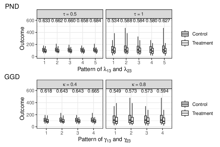
Illustration of conditional distributions and treatment effects. Figure 1 displays the distributions at the final time point () under the alternative hypothesis for each shape-parameter pattern and scale parameter setting, evaluated at a representative baseline value.
The shape-parameter patterns were designed to represent qualitatively different forms of treatment effects beyond simple location shifts. In Pattern 1, the treatment group exhibits a more favorable median outcome; however, its distribution has a heavier upper tail, indicating that the treatment effect diminishes or may even become unfavorable among more severe cases. In contrast, in the final pattern (Pattern 5 for PND and Pattern 4 for GGD), the treatment effect is reflected not only in an improved median but also in a lighter upper tail, indicating an amplified benefit among more severe cases. In the remaining patterns, the shape parameters at the final time point are identical across groups, so that between-group differences are primarily driven by location rather than distributional shape.
Except for Pattern 3 in the PND scenarios, the shape parameters vary over time, and thus the assumption of shape invariance across time points underlying BCMMRM is violated. Pattern 3 corresponds to the special case , for which the distribution reduces to a log-normal distribution at all time points.
Correlation structure. Within-participant longitudinal dependence was characterized by an AR(1) structure with correlation parameter . In the PND setting, this correlation structure is inherent to the definition of the multivariate PND on the transformed scale. In the GGD setting, dependence was introduced via a multivariate normal copula with AR(1) correlation, which was subsequently transformed to obtain GGD marginals.
Missing-data mechanism. Dropout due to insufficient treatment effect was incorporated through a logistic regression–based missing-at-random (MAR) mechanism. The dropout probability depended on the most recent observed outcome: on the Box–Cox transformed and scaled (unit standard deviation) outcome in the PND setting, and on the scaled outcome without transformation in the GGD setting. The intercept parameter was calibrated so that the overall dropout rate across both groups was approximately 30% at the final time point. Because the dropout mechanism depended only on observed past outcomes, the MAR assumption was satisfied. Missing values were generated solely through dropout, resulting in a monotone missing data pattern. In addition, for reference, we have also set a scenario with 0% dropout.
Analysis procedures. Each simulation scenario was replicated times. For each simulated dataset, a conventional MMRM assuming normality (used for hypothesis testing only), BCMMRM, BCMVR based on the median difference [BCMVR(M)], and BCMVR based on the probability-based measure [BCMVR(P)] were applied. In all analyses, baseline was included as a covariate. For the conventional MMRM, the baseline outcome on the original scale was included, together with its interaction with time. An unstructured covariance matrix was assumed for the repeated measurements, and the Kenward–Roger method [9] was used for degree-of-freedom adjustment. For BCMMRM and BCMVR, the baseline outcome after the Box–Cox transformation was included as a covariate, and for BCMMRM its interaction with time was also included. This specification was adopted to maintain consistency with the scale on which each model was formulated. In particular, BCMMRM and BCMVR model the transformed outcome, and therefore including the transformed baseline provides a covariate representation aligned with the transformed-scale model. In the simulation settings, the baseline covariate followed a log-normal distribution, so that the inverse transformation of its mean on the transformed scale coincided with its median on the original scale. Thus, conditioning on the mean of the transformed baseline corresponded to conditioning on the median of the baseline on the original scale. In addition, their small-sample adjusted versions described in Section 3.3 were also applied, denoted as BCMVR(M)a and BCMVR(P)a.
For BCMMRM, BCMVR(M), and BCMVR(M)a, inference was performed for the median difference at the final time point, including a two-sided hypothesis test of
at significance level and construction of a confidence interval.
For BCMVR(P) and BCMVR(P)a, inference was performed for the probability-based treatment effect at the final time point, including a two-sided hypothesis test of
at significance level and construction of a confidence interval.
Performance measures. Simulation performance was evaluated in terms of empirical type I error rates under the null hypothesis and empirical power under the alternative hypothesis, empirical bias of the estimated treatment effect, and empirical coverage probabilities of the nominal confidence intervals. Furthermore, we evaluated the proportion of simulations in which the BCMVR model was selected over the BCMMRM model based on a likelihood ratio test, where BCMMRM and BCMVR correspond to the null and alternative hypotheses, respectively, at a significance level of 0.05. This comparison serves as a diagnostic for detecting differences in distributional shape between treatment groups. As an additional measure of estimation accuracy, we evaluated the ratio of the average estimated standard errors to the standard deviation of estimated treatment effects across simulation replicates, multiplied by 100. Values close to 100 indicate small bias in the standard errors, whereas values below and above 100 indicate underestimation and overestimation of the standard errors, respectively. In addition, we recorded the convergence rate of the estimation algorithm for the BCMVR model in each simulation scenario. For all performance measures other than the convergence rate, simulation replicates in which the BCMVR estimation algorithm failed to converge were excluded from the evaluation.
Software. All simulations were conducted using R (version 4.6.0; R Core Team, Vienna, Austria) and several R packages. The MMRM analyses were performed using the mmrm package [10], while the BCMMRM analyses were conducted using the bcmixed package [3]. The proposed BCMVR method was implemented using the bcmvr package [11]. Multivariate power-normal random variables were generated using the powerNormal package [12], and generalized gamma random variables were generated using the flexsurv package [13].
4.2 Simulation results
In this section, we present the simulation results under the 30% dropout setting. Results for the no-dropout setting, together with additional simulation results (SE ratio, coverage), are provided in the Supporting Information.
| Dist. | Scale | Null scenarios | Alternative scenarios | |||||||
| 1 | 2 | 3 | 4 | 5 | ||||||
| PND | 0.5 | 25 | ||||||||
| 50 | ||||||||||
| 100 | ||||||||||
| 1.0 | 25 | |||||||||
| 50 | ||||||||||
| 100 | ||||||||||
| GGD | 0.4 | 25 | – | – | ||||||
| 50 | – | – | ||||||||
| 100 | – | – | ||||||||
| 0.8 | 25 | – | – | |||||||
| 50 | – | – | ||||||||
| 100 | – | – | ||||||||
Model selection between BCMMRM and BCMVR. Table 1 shows the proportion of simulations in which the BCMVR model was selected over the BCMMRM model based on the likelihood ratio test comparing the BCMMRM model (null hypothesis) and the BCMVR model (alternative hypothesis). We first describe the results under the alternative scenarios with treatment effects.
Under the PND data-generating mechanisms, the BCMVR model was selected more frequently in patterns 1 and 5, where the shape parameter differed between treatment groups as well as across time points. In contrast, the selection proportion was low in patterns 2–4, where differed only across time points but not between groups. In addition, the selection proportion increased as the scale parameter became larger.
Under the GGD scenarios, a similar dependence on the shape parameter patterns was observed, with higher selection proportions in patterns 1 and 4 where the shape parameter differed between treatment groups. In contrast to the PND scenarios, the scale parameter had little impact on the model selection results.
Under the null scenarios with no treatment effect, the selection proportions were broadly similar to those observed in scenarios 2–4 for the PND settings and scenarios 2–3 for the GGD settings.
These results suggest that the likelihood ratio test can detect model misspecification caused by group-specific differences in distributional shape, although the detection ability becomes limited when the sample size is small. In scenarios where the BCMMRM model was correctly specified, the empirical type I error rates approached the nominal significance level as the sample size increased.
In scenarios without missing data, the selection rate of BCMVR increased under the alternative hypothesis, while under the null hypothesis it became closer to the nominal significance level (Table S1).

Empirical type I error. The empirical type I error rates are shown in Figure 2. Inflation of the type I error rate was observed when the scale parameters were small (i.e., small in PND and small in GGD) and the sample size per group was for the proposed methods. In these settings, the degree of inflation was substantial and the empirical small-sample adjustment described in Section 3.3 was not sufficient to fully control the nominal level. In the other scenarios, however, the small-sample adjustment maintained the nominal significance level. In contrast, the asymptotic method showed slight inflation when the sample size per group was . Based on these results, the following comparisons focus on the small-sample adjusted procedures.
| Dist. | Scenario | Min. | Q1 | Median | Q3 | Max. |
|---|---|---|---|---|---|---|
| PND | , | 87.3 | 89.9 | 92.2 | 93.8 | 96.3 |
| PND | Other | 99.2 | 99.8 | 100.0 | 100.0 | 100.0 |
| GGD | , | 91.3 | 91.8 | 93.6 | 95.2 | 95.7 |
| GGD | Other | 99.4 | 99.8 | 100.0 | 100.0 | 100.0 |
Summary statistics of the convergence rates of the estimation algorithm for the BCMVR model across all simulation scenarios, including those generated under the alternative hypothesis, are presented in Table 2. Lower convergence rates were observed when and the scale parameters were small (i.e., for PND and for GGD). In the other scenarios, the algorithm converged in almost all simulation runs. Notably, these settings largely coincide with those in which inflation of the type I error rate was observed.
In scenarios without missing data, the inflation of the type I error rate for BCMVR observed in small-sample settings was attenuated (Figure S6).

Empirical bias of treatment effect. The bias of treatment effect under the alternative hypothesis is shown in Figure 3. For the BCMMRM method, little bias was observed in scenarios where the shape parameters differed only across time points but not between treatment groups (PND patterns 2 and 4, and GGD patterns 2 and 3). In contrast, when the shape parameters differed between treatment groups at the time point of interest (PND patterns 1 and 5, and GGD patterns 1 and 4), noticeable bias was observed.
In comparison, the BCMVR method showed negligible bias for both the median difference and the probability-based measure across all scenarios, including those generated from the GGD model where the BCMVR model was misspecified.

Under the null hypothesis, virtually no bias was observed in any situation or method (Figure S1).
In scenarios without missing data, convergence rates were slightly improved (Table S2).
Empirical power. The empirical power of the tests is shown in Figure 4. The BCMMRM method generally showed high power across many scenarios. However, this tendency partly reflects the bias observed in the estimated treatment effects when the shape parameters differed between treatment groups.
The conventional MMRM achieved relatively high power in scenarios with small sample sizes () and/or mild skewness (e.g., or ). However, in other scenarios, the power was rather reduced.
The BCMVR(M) method showed relatively stable power across scenarios, although the power was generally lower than that of the BCMMRM method.
The BCMVR(P) method showed power levels between those of BCMMRM and BCMVR(M), indicating a moderate trade-off between robustness and efficiency.
Although statistical power generally increased in scenarios without missing data, the relative differences between the methods were similar to those observed in the presence of missing data (Figure S7).
SE ratio. The ratios of the model-based standard errors to the empirical standard deviations are presented in Figures S2–S3. For both BCMVR methods, standard errors tended to be underestimated when the sample size was small () and the scale parameter was small. This finding was consistent with the observed inflation of the type I error rate under these settings.
For the generalized gamma distribution with and , some underestimation was observed for the standard errors of BCMVR(M). However, this was primarily attributable to the heavy-tailed distribution of the median difference estimator, which inflated its empirical standard deviation, and therefore had little impact on the observed type I error rate. Apart from these settings, the standard error estimates were generally unbiased.
In contrast, BCMMRM exhibited a slight tendency to underestimate standard errors in scenarios where the distributional shapes differed between treatment groups.
When no missing data were present, the bias of SE for the proposed methods was attenuated (Figures S10–S11).
Empirical coverage probability. The empirical coverage probabilities of the nominal confidence intervals are shown in Supplementary Figures S4-5. For the BCMMRM method, the coverage probabilities tended to fall below the nominal level in scenarios where noticeable bias was observed in the estimated treatment effects, as expected from the bias results.
In contrast, the proposed BCMVR methods generally maintained coverage close to the nominal level across most scenarios. Under the smallest sample size () with small scale parameters, the coverage probabilities were slightly below the nominal level, which is consistent with the type I error inflation observed in these settings.
In the absence of missing data, the empirical coverage probabilities of the proposed methods were closer to the nominal level (Figures S12–S13).
4.3 Application to ACTG 193A trial data
To illustrate the proposed methods, we analyzed data from the AIDS Clinical Trial Group (ACTG) 193A study [14, 15] which is available in the bcmixed R package. The study was a randomized clinical trial evaluating antiretroviral treatment strategies in patients with advanced HIV infection. CD4 cell counts were measured at weeks 8, 16, 24, and 32.
In the present analysis, we considered two treatment groups: the two-drug regimen (zidovudine + didanosine), denoted by , and the three-drug regimen (zidovudine + didanosine + nevirapine), denoted by . The comparison focuses on evaluating the add-on effect of nevirapine.
The sample sizes were and for the two-drug and three-drug groups, respectively. At week 32, the numbers of observed outcomes were 187 (63.8%) in the two-drug group and 208 (67.5%) in the three-drug group.

Figure 5 shows the distributions of CD4 cell counts (shifted by adding 1 to avoid zero values) at weeks 8, 16, 24, and 32 in the two treatment groups. The distributions appear markedly right-skewed at all visits, supporting the use of transformation-based modeling approaches and distribution-sensitive treatment effect summaries.
We applied BCMMRM, BCMVR(M), and BCMVR(P) to estimate the treatment effect at week 32. As in the simulation study, the baseline outcome after the Box–Cox transformation was included as a covariate. In the simulation studies and throughout this paper, smaller outcome values are assumed to represent better clinical status. However, for the CD4 cell count data, larger values indicate better clinical status. Therefore, the direction of inequality in equation (1) is reversed in this application.
The likelihood ratio test comparing BCMMRM and BCMVR yielded a -value of 0.021, suggesting potential differences in distributional shape between the treatment groups. The estimated shape parameter under BCMMRM was . Under BCMVR, the estimated shape parameters were for the two-drug group () and for the three-drug group (). These estimates suggest some differences in distributional shape between the two treatment groups.
BCMMRM estimated a median difference of 6.46 (95% CI: 3.16 to 9.76, ). BCMVR(M) estimated a median difference of 4.89 (95% CI: 1.54 to 8.25, ). The probability-based measure BCMVR(P) estimated that the probability that a randomly selected patient in the three-drug group has a higher CD4 count than a patient in the two-drug group was 0.585 (95% CI: 0.534 to 0.635, ).
Overall, the BCMVR framework provides complementary perspectives on treatment effects through distributional summaries while accommodating potential differences in distributional shape between treatment groups.
5 Discussion
In this study, we proposed the BCMVR framework for treatment effect inference in longitudinal clinical trial data with potentially skewed outcome distributions. The proposed approach extends the conventional BCMMRM framework by enabling inference based on interpretable distributional summaries, including the median difference and a probability-based treatment effect measure.
The simulation results demonstrated that the conventional BCMMRM approach can produce biased estimates of treatment effects when the underlying outcome distributions differ in shape between treatment groups. In contrast, the BCMVR procedures provided nearly unbiased estimation across all considered scenarios, including those under model misspecification with generalized gamma data-generating mechanisms. These findings suggest that BCMVR offers a more robust alternative when distributional heterogeneity exists.
Regarding hypothesis testing, BCMMRM generally exhibited high statistical power; however, this was partly attributable to bias under model misspecification. The BCMVR(M) procedure showed relatively stable but moderate power, whereas BCMVR(P) tended to achieve power levels between those of BCMMRM and BCMVR(M), suggesting a useful balance between robustness and efficiency.
The likelihood ratio test comparing BCMMRM and BCMVR provided informative diagnostics for detecting distributional misspecification. In scenarios with differing shape parameters between treatment groups, the BCMVR model was selected more frequently. However, the selection proportion was modest in small-sample settings, likely reflecting estimation instability and reduced convergence associated with the increased model complexity of BCMVR. Consistent with this, the simulation results showed reduced estimation accuracy and lower convergence rates when both the sample size and scale parameters were small. In practice, the advantages of BCMVR may become more evident when the sample size per group is approximately 50 or larger.
Taken together, these results suggest that BCMVR(P) can be recommended as a practical default procedure. The probability-based treatment effect provides a favorable balance between robustness and efficiency while remaining clinically interpretable. However, when the sample size is small and substantial differences in distributional shape are unlikely, the conventional BCMMRM approach may still offer more stable inference due to its simpler structure.
Importantly, the BCMVR framework should not be viewed merely as an exploratory tool but as a unified inferential framework based on distributional summaries of longitudinal outcomes. In particular, the probability-based measure integrates information over the entire marginal distributions and can capture differences beyond central tendency. In skewed distributions, the mean may provide a limited representation of the outcome, and even the median may fail to adequately reflect group differences when distributional shapes differ between treatment groups. In such settings, the probability-based measure offers a more comprehensive assessment of treatment effects. The proposed framework is related to probabilistic indices such as the Mann–Whitney parameter and the probability of superiority, but extends these ideas to longitudinal clinical trial settings with potentially skewed outcomes and missing observations under MAR. By combining the Box–Cox transformation with a parametric multivariate regression framework, BCMVR provides a flexible yet unified modeling approach that enables covariate-adjusted inference for both median-based and probability-based treatment effects within the same longitudinal framework.
From a clinical perspective, such distributional summaries may offer intuitive measures of treatment benefit. Depending on the direction of the outcome, the probability-based measure can be interpreted as the probability that a randomly selected patient from the treatment group has a better outcome than a randomly selected patient from the control group. This interpretation may be easier to communicate to clinicians than summaries based solely on a single summary measure such as the mean or median.
To facilitate practical implementation, we provide an R package, bcmvr, implementing the proposed framework. The package is available at https://github.com/kzkzmr/bcmvr. Detailed usage and examples are provided in the GitHub repository and in the package documentation (accessible via ?bcmvr in R). The package can be installed using standard tools (e.g., remotes::install_github("kzkzmr/bcmvr")).
The choice of the Box–Cox transformation and the PND can be justified from both empirical and theoretical perspectives. Previous work [7] has shown that the PND provides a good fit across a wide range of clinical laboratory measurements. Furthermore, the Box–Cox formulation ensures that the conditional distribution of the outcome given covariates remains within a tractable family (PND), enabling closed-form or easily computable expressions for clinically interpretable quantities such as median differences and probability-based measures. This property stems from the fact that, after transformation, the outcome follows a multivariate normal model, whose conditional distribution is well characterized through linear structures. In this sense, the approach effectively leverages the tractability of the normal distribution under linear operations. In contrast, models that specify a particular marginal distribution—such as the GGD—do not generally preserve this closure property, as the corresponding conditional distribution given covariates typically falls outside the assumed family, thereby complicating inference for such measures. This structural advantage is particularly important when inference targets are defined through conditional distributions, rather than marginal summaries alone. Importantly, the proposed framework is not restricted to the PND but can be extended to other flexible distributional families, highlighting that its primary contribution lies in the inferential framework rather than in the specific choice of distribution.
Several limitations should be noted. First, the simulation settings considered only a limited range of longitudinal structures and outcome distributions. Broader evaluations under more complex designs and additional distributional families would further clarify the operating characteristics of the proposed methods. In addition, because BCMVR introduces group- and time-specific transformation parameters, estimation may become unstable in small samples. In particular, performance deteriorated when both the sample size and scale parameters were small, as reflected in type I error inflation and reduced convergence rates. One possible explanation is that the flexibility of BCMVR increases the number of nuisance parameters relative to the available information. In the present setting, the transformed outcomes may exhibit time-specific variances induced by the group- and time-specific transformation parameters, making simple covariance structures such as compound symmetry difficult to justify. Consequently, more flexible covariance structures, such as unstructured covariance matrices, are often required, potentially leading to unstable covariance estimation in small samples. Furthermore, the first-order approximation underlying the delta method may be insufficient for nonlinear treatment effect measures, particularly when dropout further reduces the effective information size. Another limitation is that the proposed treatment effect is defined conditionally on covariates being fixed at their overall sample means. In randomized clinical trials, marginal or covariate-standardized probability-based estimands may also be of interest because they provide population-level summaries of treatment effects. Extending the proposed framework to accommodate such marginal interpretations represents an important direction for future research. Furthermore, although the present study focused on randomized clinical trials, the proposed framework may also be applicable to observational studies through appropriate adjustment for confounding covariates. Investigation of causal and marginal interpretations of the probability-based measure in observational settings is another important topic for future work.
Overall, the BCMVR framework extends conventional MMRM and BCMMRM methodologies by enabling treatment effect inference based on interpretable distributional summaries while accommodating differences in distributional shape. This provides a flexible approach for analyzing longitudinal clinical trial data when outcome distributions deviate from standard normality assumptions.
Funding
This work was supported by JSPS KAKENHI Grant Numbers 23K11003 and 26K02873.
Author Contributions
Kazushi Maruo conceived the study, developed the methodology, conducted the analyses, and drafted the manuscript. Ryota Ishii and Yusuke Yamaguchi reviewed the manuscript and verified the analytical results. Toshio Shimokawa, Tomoyuki Sugimoto, and Masahiko Gosho reviewed the manuscript and provided supervision. All authors approved the final version of the manuscript.
Financial Disclosure
None reported.
Conflicts of Interest
The authors declare no conflicts of interest.
References
- [1] (2001) Accounting for dropout bias using mixed-effects models. Journal of Biopharmaceutical Statistics 11 (1–2), pp. 9–21. External Links: Document Cited by: §1.
- [2] (2017) Interpretable inference on the mixed effect model with the Box–Cox transformation. Statistics in Medicine 36 (15), pp. 2420–2434. External Links: Document Cited by: §1, §3.3.
- [3] (2021) Bcmixed: A package for median inference on longitudinal data with the Box–Cox transformation. The R Journal 13 (2), pp. 253–265. External Links: Document, ISSN 2073-4859 Cited by: §1, §4.1.
- [4] (1964) An analysis of transformations. Journal of the Royal Statistical Society, Series B 26 (2), pp. 211–252. External Links: Document Cited by: §1.
- [5] (1980) Some properties of the power normal distribution. Japanese Journal of Biometrics 1, pp. 28–54. External Links: Document Cited by: §3.2.
- [6] (1990) Small-sample adjustments to tests with unbalanced repeated measures assuming several covariance structures. Journal of Statistical Computation and Simulation 37 (1–2), pp. 69–87. External Links: Document Cited by: §3.3.
- [7] (2017) Statistical simulation based on right skewed distributions. Computational Statistics 32, pp. 889–907. External Links: Document Cited by: §4.1, §5.
- [8] (1974) A log gamma model and its maximum likelihood estimation. Biometrika 61 (3), pp. 539–544. External Links: Document Cited by: §4.1.
- [9] (1997) Small sample inference for fixed effects from restricted maximum likelihood. Biometrics 53 (3), pp. 983–997. External Links: Document Cited by: §4.1.
- [10] (2025) Mmrm: mixed models for repeated measures. Note: R package version 0.3.16 External Links: Link, Document Cited by: §4.1.
- [11] (2026) Bcmvr: treatment effect inference using box-cox multivariate regression. Note: R package version 0.1.0 External Links: Link Cited by: §4.1.
- [12] (2026) PowerNormal: the power normal distribution with or without reparametrization. Note: R package version 0.1.0 External Links: Link Cited by: §4.1.
- [13] (2016) Flexsurv: a platform for parametric survival modeling in R. Journal of Statistical Software 70 (8), pp. 1–33. External Links: Document Cited by: §4.1.
- [14] (1998) A randomized, controlled, double-blind study comparing the survival benefit of four different reverse transcriptase inhibitor therapies (three-drug, two-drug, and alternating drug) for the treatment of advanced AIDS. AIDS Clinical Trial Group 193A Study Team. Journal of Acquired Immune Deficiency Syndromes and Human Retrovirology 19 (4), pp. 339–349. External Links: Document Cited by: §4.3.
- [15] (2011) Applied longitudinal analysis. 2 edition, Wiley, New York. External Links: Document Cited by: §4.3.
Supporting information material for
“A flexible framework for treatment effect inference in longitudinal clinical studies with skewed outcomes”
Kazushi Maruo∗, Ryota Ishii, Yusuke Yamaguchi,
Toshio Shimokawa, Tomoyuki Sugimoto, and Masahiko Gosho
∗kazushi.maruo@gmail.com
S1 Hessian matrix of the log-likelihood:
For notational conventions, see Section 2.1. The Hessian matrix of the log-likelihood is
The components of the Hessian matrix are given as follows.
– block.
where denotes the indicator function, which takes the value 1 if the condition inside the parentheses is satisfied and 0 otherwise, denotes the set of participants for whom the outcomes are observed at all time points involved in the corresponding subscript(s), and denotes a vector of the same dimension as whose component corresponding to time (i.e., the position of the observation at time in ) is equal to if observed, and zero otherwise. In addition,
– block.
– block.
where
Cross blocks.
S2 Outer product matrix of score function:
The matrix is defined as
where is the log-likelihood for the -th participant. The components of the matrix are given as follows.
– block.
– block.
– block.
Cross blocks.
S3 Gradient vector for median function
The gradient vector for the median function, , is given by
where denotes the th canonical basis vector in , that is, a vector with 1 in the th position and 0 elsewhere, and denotes a zero vector of length .
S4 Gradient vector for the logit-transformed probability-based effect measure
The gradient vector for the logit-transformed probability-based effect measure is given by
The components are given as follows.
These components are evaluated using numerical integration.
S5 Additional simulation results under 30% dropout
Bias of treatment effect under null hypothesis

Standard error ratio


Empirical coverage probability


S6 Complete simulation results under no dropout
Model selection between BCMMRM and BCMVR
| Dist. | Scale | Null scenarios | Alternative scenarios | |||||||
|---|---|---|---|---|---|---|---|---|---|---|
| 1 | 2 | 3 | 4 | 5 | ||||||
| PND | 0.5 | 25 | ||||||||
| PND | 0.5 | 50 | ||||||||
| PND | 0.5 | 100 | ||||||||
| PND | 1.0 | 25 | ||||||||
| PND | 1.0 | 50 | ||||||||
| PND | 1.0 | 100 | ||||||||
| GGD | 0.4 | 25 | – | – | ||||||
| GGD | 0.4 | 50 | – | – | ||||||
| GGD | 0.4 | 100 | – | – | ||||||
| GGD | 0.8 | 25 | – | – | ||||||
| GGD | 0.8 | 50 | – | – | ||||||
| GGD | 0.8 | 100 | – | – | ||||||
Convergence rates
| Dist. | Scenario | Min. | Q1 | Median | Q3 | Max. |
|---|---|---|---|---|---|---|
| PND | , | 95.2 | 96.0 | 96.6 | 96.7 | 97.1 |
| PND | Other | 99.2 | 100.0 | 100.0 | 100.0 | 100.0 |
| GGD | , | 98.2 | 98.2 | 98.2 | 98.2 | 98.4 |
| GGD | Other | 99.7 | 100.0 | 100.0 | 100.0 | 100.0 |
Empirical type I error

Empirical power

Bias of treatment effect


Standard error ratio


Empirical coverage probability

