The Transient Counting Statistics of Autonomous Quantum Clocks

The Hamiltonian of the two-level quantum emitter is chosen to be ($\hbar=1$)

where $\ket{e}$ denotes the excited state of the two-level system, and we assume that the frequency $\Omega$ is experimentally accessible through resonance fluorescence measurement with an ideal photodetector. To fuel the emitter using minimal thermodynamic resources, we assume that the two-level system undergoes dephasing along the axis defined by the Hermitian observable $\hat{X}$, described by the master equation $\frac{d\hat{\rho}}{dt}=-i[\hat{H},\hat{\rho}]-\gamma_{m}[\hat{X},[\hat{X},\hat{\rho}]]$. Equivalently, the same dynamics can be engineered via continuous weak measurement of $\hat{X}$ on the two-level system at measurement rate $\gamma_{m}$ [42, 2], provided that the measurement record is discarded such that the resulting evolution is unconditional. We consider a one-parameter generalization of the choice $\hat{X}=\hat{\sigma}_{x}$ used in Refs. [42, 2],

The fluorescence-monitored qubit is governed by the interplay between the energy basis $\{|g\rangle,|e\rangle\}$ and the noise basis defined by the eigenstates of $\hat{X}(\theta)$. The angle $\theta$ parametrizes this misalignment, ranging from aligned bases at $\theta=\pi/2$ ($\hat{X}=\hat{\sigma}_{z}$) to maximal misalignment at $\theta=0$ ($\hat{X}=\hat{\sigma}_{x}$). This mismatch fully determines the steady state, including the emergence of energy-basis coherences.

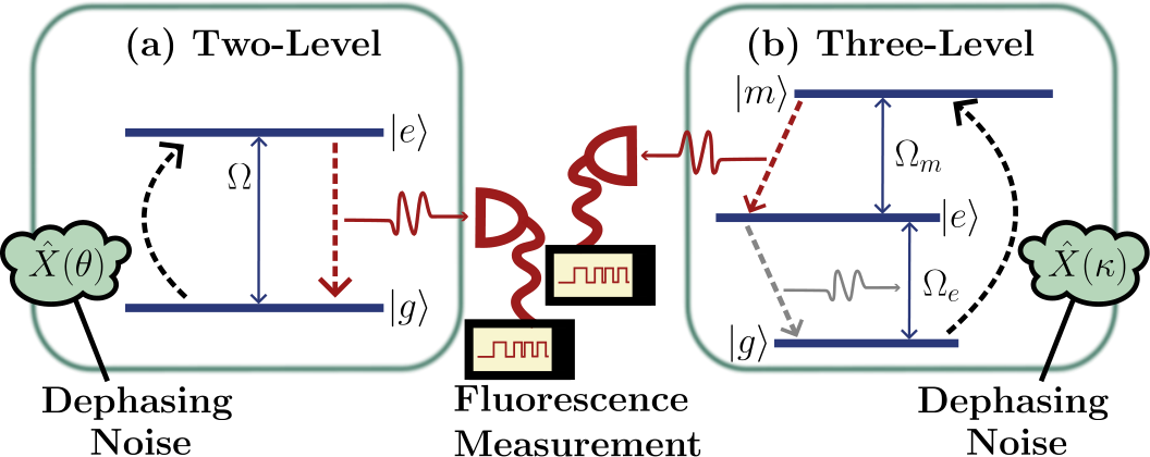
The clock signal is obtained from a detector counting fluorescence emission between the two levels, where the detector integration time $dt$ is much smaller than $\gamma_{w}^{-1}$, $\gamma_{w}$ being the spontaneous emission rate. In other words, we assume that the integration time is much shorter than the characteristic decay time from the excited to the ground state (see Fig. 1 for a schematic of the fluorescence and dephasing setup).

The tilted Liouvillian of the two-level system relevant for obtaining the counting statistics is given by

where $\hat{L}_{w}=\hat{\sigma}_{-}=\ket{g}\bra{e}$ and $\hat{L}_{w}^{\dagger}=\hat{\sigma}_{+}=\ket{e}\bra{g}$.

To understand the dynamics let us set the tilt $s=0$ and write the density matrix in terms of its Bloch components, $\hat{\rho}=\frac{1}{2}\left(\hat{\mathds{1}}+x\hat{\sigma}_{x}+y\hat{\sigma}_{y}+z\hat{\sigma}_{z}\right)$, with $z=p_{e}-p_{g}$, so that Eq. (23) becomes

with $\zeta=\frac{1}{2}\gamma_{w}+4\gamma_{m}$. Let us first build an intuition for the dynamics. Ignoring the coherences, Eq. (26) shows that the dephasing operator $\hat{X}$ induces the population dynamics,

where $\epsilon(\theta)$ is the noise-induced transition rate. Note that it is the $\hat{\sigma}_{x}$ component of $\hat{X}$ that drives transitions between $|g\rangle$ and $|e\rangle$; the noise is the only mechanism able to populate the excited state, since the Hamiltonian is diagonal in the energy basis. In this simplified picture, the rate equation in Eq. (27) yields the steady-state population $p_{e}^{\rm ss}\to\frac{\epsilon(\theta)}{2\epsilon(\theta)+\gamma_{w}}$.

However, the same noise process that induces population transitions also creates coherences. The crucial term is the source $2\gamma_{m}\sin(2\theta)\,z$ in Eq. (24): a noise kick acting on a state with population imbalance ($z\neq 0$) generates a coherence (except at $\theta=\{0,\frac{\pi}{2}\}$). The dephasing in turn damps this coherence, both directly, through the rate $4\gamma_{m}\sin^{2}\theta+\frac{\gamma_{w}}{2}$ acting on the $x$ quadrature, and indirectly, through the Hamiltonian precession, which rotates $x$ into the orthogonal quadrature $y$ where it is damped at the rate $\zeta$, opening an additional channel for coherence decay. What makes this scenario non-trivial is that these coherences are not merely a by-product of the dynamics: they feed back on the populations, entering through the term $2\gamma_{m}\sin(2\theta)\,x$ in Eq. (26).

Solving the stationary Bloch equations exactly, we obtain the steady state,

where the excited-state population is

with

The coherence feedback renormalizes the population dynamics with the effective rate $\epsilon_{\rm eff}(\theta)$. The suppression factor $R(\theta)\in(0,1]$ thus captures the net effect of the coherence feedback on the stationary population. The simple rate-equation picture ($R\to 1$) is recovered in two limits: at $\theta=0$, where no coherence is generated, and for $\Omega^{2}\gg\gamma_{m}\zeta$, where rapid precession drains the coherence before it can feed back.

Finally, the steady-state coherences are

where

This makes the origin of the off-diagonal elements in Eq. (28) explicit: the coherence $x=\chi(\theta)\,z$ is nonzero whenever the population is imbalanced ($z\neq 0)$ and the noise axis is tilted ($\sin(2\theta)\neq 0$).

To characterize the statistics of the quantum jumps we now consider the tilted dynamics with $s\neq 0$. We evaluate the mean number of clicks $\langle N\rangle_{t}$ and their variance $\mathrm{Var}(N)_{t}=\langle N^{2}\rangle_{t}-\langle N\rangle_{t}^{2}$ as functions of $\theta$. The tick statistics are further characterized by the Mandel $Q_{t}$ parameter [40], $Q_{t}=\frac{\langle N^{2}\rangle_{t}-\langle N\rangle_{t}^{2}}{\langle N\rangle_{t}}-1$, which quantifies deviations from Poissonian statistics ($Q_{t}=0$). At finite $t$, it depends strongly on the initial state, with a marked difference between preparing the system in the ground state (Fig. 2) and in the excited state (Fig. 3). In both cases, the leading time-extensive term predicted by LDT fails to reproduce the exact simulations of quantum jumps using the operator sum (Kraus) representation. Agreement is only recovered by including the transient contributions.

As observed in Figs. 2 and 3, the leading-order LDT prediction yields a vanishing mean emission rate as $\theta\to\pi/2$. This follows from the stationary emission rate, $k_{\rm ss}(\theta)=\gamma_{w}p_{e}^{\rm ss}(\theta)$. Although $R(\theta)$ remains finite as $\theta\to\pi/2$, the effective pump scales as $\epsilon_{\rm eff}\propto\cos^{2}\theta$. The emission rate is therefore increasingly pump-limited as $\theta$ approaches $\pi/2$, and vanishes exactly at $\theta=\pi/2$ where the noise-induced pumping is switched off. Once the qubit decays it can never be re-excited.

From the perspective of the tilted Liouvillian, this behavior is reflected in the fact that, at $\theta=\pi/2$, the spectrum becomes independent of $s$. In particular, the dominant eigenvalue satisfies $\lambda_{\rm dom}(s)=0$ for all $s$, implying that all time-extensive cumulant rates vanish and the LDT carries no information. All $s$-dependence of the counting statistics is instead encoded in the prefactor $c_{\rm dom}(s)=p_{e}(0)\,e^{-s}+p_{g}(0)$, i.e., in the eigenvectors of $\hat{\mathcal{L}}_{s}$. Consequently, the outcome depends crucially on the initial-state preparation.

Near $\theta=\pi/2$, the steady state approaches the ground state. A system prepared in $|g\rangle$ therefore starts arbitrarily close to the steady state, and since the ground state produces no emission, both the mean count, $\langle N\rangle_{\infty}\to 0$, and transient contributions vanish (since $c_{\rm dom}(s)\to 1$). In this case, the leading-order and corrected predictions around $\theta=\pi/2$ coincide (Fig. 2).

By contrast, a system prepared in $|e\rangle$ is initially maximally far from the steady state. At $\theta=\pi/2$, it emits exactly one photon before falling dark, giving $\langle N\rangle_{\infty}=1$ given sufficient time, as shown in Fig. 3. Note that maximally sub-Poissonian statistics ($Q_{t}\rightarrow-1$) here cannot be equated with maximal accuracy, since it means a near-deterministic count (one click) given sufficient time, rather than regular ticks. We return to this in Subsection IV.1.

We can alternatively fix the angle, for instance to ${\theta=0}$, which both yields simple analytical expressions (there are no coherences) and lets us examine the behaviour as the monitoring strength $\gamma_{m}$ is varied. For the ground state as the initial state, the average number of clicks $\langle N\rangle_{t}={\langle N\rangle_{t}}_{\mathrm{LDT}}+{\langle N\rangle}_{\mathrm{early}}^{(g)}$ is

where the second term is the transient contribution from the initial state. Similarly, the variance $\mathrm{Var}(N)_{t}=\mathrm{Var}_{\mathrm{LDT}}(N)_{t}+\mathrm{Var}_{\mathrm{early}}^{(g)}(N)$ reads

and the Mandel $Q^{(g)}_{t}$ parameter is

These quantities are shown as functions of $\gamma_{m}$ in Fig. 4. Here the initial-state dependence is erased at strong dephasing. The ground- and excited-state predictions (discussed below) differ at weak dephasing but converge as $\gamma_{m}$ grows, both approaching the leading-order result. A large $\gamma_{m}$ makes the pumping and relaxation fast, so the system reaches its steady state almost immediately and the transient contributions are over before an appreciable number of photons has been counted. The system forgets its preparation quickly, and the transient contributions (which measure the distance of the initial state from stationarity) become negligible relative to the time-extensive term.

For an excited-state initial condition (Fig. 5), the deviation from the leading-order prediction is much stronger than for the ground state. The average number of clicks is $\langle N\rangle_{t}={\langle N\rangle_{t}}_{\mathrm{LDT}}+{\langle N\rangle}_{\mathrm{early}}^{(e)}$, with the same time-extensive term (33) and

Note that this correction is positive, in contrast to the ground-state case: an excited qubit emits more during its transient than a stationary one, producing an excess of early counts. The variance correction is

and the Mandel $Q_{t}^{(e)}$ parameter reads as

At weak dephasing, $\gamma_{m}\to 0$, the pump vanishes and the excited qubit emits a single photon before relaxing to the ground state, so $Q_{t}^{(e)}\to-1$, the same near-deterministic limit reached when the dephasing is aligned with the energy basis. Here, this limit is approached instead by switching off the dephasing noise.

The transient contributions in Eqs. (18) and (19) are constants: they are evaluated for a fixed initial state $|\rho(0)\rangle\!\rangle$ and represent the offset that the transient relaxation imprints on the long-time counting statistics. For the mean, this contribution vanishes when the system is prepared in the steady state, $|\rho(0)\rangle\!\rangle=|\rho_{\rm ss}\rangle\!\rangle$ (see Eq. (28)), since there is then no transient to relax through. In this case the mean correction exactly vanishes, $\langle N\rangle_{\rm early}^{(ss)}=0$, and the leading-order LDT prediction reproduces the mean number of jumps exactly. The variance correction, however, does not vanish, but converges to the small residual offset,

giving a Mandel parameter $Q_{t}^{(ss)}$ with

This residual is the stationary boundary contribution to the variance discussed in Sec. II.

The excellent agreement between the analytical expressions and the simulations demonstrates that these asymptotic expansions capture the relevant dynamics over the parameter regimes considered. The counting window used in the simulations is sufficiently long to reach the regime where the expansions apply, $t\gg\tau_{\rm relax}$, with $\tau_{\rm relax}$ set by the slowest mode of $\hat{\mathcal{L}}_{0}$ populated by the initial state. At $\theta=0$, both $\hat{\sigma}_{x}$ and the Hamiltonian preserve the populations, so the diagonal preparations used here remain within the population sector and relax at the single rate $\Gamma=4\gamma_{m}+\gamma_{w}$. Outside their range of validity, the truncated expansions can exhibit pathologies, such as a negative variance. For the ground state, $\mathrm{Var}_{\mathrm{LDT}}(N)_{t}+\mathrm{Var}^{(g)}_{\rm early}(N)$ becomes negative for $t<t^{\ast}=-\mathrm{Var}^{(g)}_{\rm early}(N)/v_{\rm ss}$, but

so the apparent negativity occurs only at times shorter than the counting window relevant for the comparison with the simulations.

Beyond the asymptotic regime, the mean and variance can be obtained in closed form at all times (see Appendix F). Subtracting the leading-order growth, $\mathcal{O}_{\rm mean}(t)=\langle N\rangle_{t}-k_{\rm ss}\,t$ and $\mathcal{O}_{\rm var}(t)=\mathrm{Var}(N)_{t}-v_{\rm ss}\,t$, isolates the subextensive part throughout the transient and shows how the initial-state contributions build up in time. Figure 6 shows this for the two-level emitter. At early times the cumulants deviate from their asymptotic growth. As the system relaxes, these deviations saturate to preparation-dependent constants that constitute the initial-state contributions central to this work.

We extend now our formalism to a three-level system. The Hamiltonian of the system is given by

where $\ket{e}$ and $\ket{m}$ are the excited states of the three-level quantum system, with $\Omega_{m}>\Omega_{e}$. We assume that $\Omega_{m}-\Omega_{e}$ is experimentally accessible, whereas $\Omega_{e}$ is not directly accessible, corresponding to losses to a reservoir via unmonitored fluorescence emission at rate $\gamma_{e}$. The fluorescence emission from the level $\ket{m}$ to the level $\ket{e}$ at rate $\gamma_{w}$ is measured as the clock transition through photodetection (see Fig. 1). Together with the dephasing operator $\hat{X}$, the tilted Liouvillian of our three-level system reads as follows:

where $\hat{L}_{w}=\ket{e}\bra{m}$ and $\hat{L}_{e}=\ket{g}\bra{e}$. It remains to specify the operator $\hat{X}$ through which the dephasing noise acts. As in the two-level case, where $\theta$ set the orientation of $\hat{X}$, we introduce a one-parameter family. Let

with $|\phi_{3}(\kappa)\rangle$ completing the orthonormal basis, and define

which annihilates $|\phi_{3}\rangle$.

The parameter $\kappa$ controls how strongly the noise couples to the emission cycle. After each emission the system is left in $|e\rangle$ and cannot emit again until it has returned to $|m\rangle$ through $|e\rangle\to|g\rangle\to|m\rangle$, the last step being driven by the $\hat{X}$-dephasing channel. Waiting for several comparable steps in sequence is more predictable than waiting for a single random one: at $\kappa=0$, where $|\phi_{1}\rangle=|e\rangle$, the noise acts directly on the post-emission state and drives the return to $|m\rangle$ efficiently, so no single step dominates the waiting time between clicks; the emission is then more regular than a memoryless process and the statistics are sub-Poissonian. As $\kappa\to 1$ the noise connects $|g\rangle$ back to $|m\rangle$ ever more weakly: the re-pumping becomes the slowest step and increasingly dominates the waiting time between clicks, causing the emission rate to collapse and the statistics to approach the Poissonian limit (see Fig. 7). At $\kappa=1$ the noise no longer acts on $|m\rangle$ at all and the emission ceases. The parameter $\kappa$ thus plays for the cascade the role that $\theta$ played for the two-level emitter.

The uncounted decay also sets when the asymptotic expressions become accurate. In the two-level emitter at $\theta=0$, for instance, the relevant relaxation was fast: a diagonal preparation relaxed at $\Gamma=4\gamma_{m}+\gamma_{w}$. In the cascade, relaxation must instead proceed through all three steps of the cycle, including the uncounted transition. The relaxation time is therefore controlled by a process invisible to the detector and can become longer when $\gamma_{e}$ is small. An observation window comfortably long in the two-level case may here be too short.

If the detected photons are regarded as the ticks of a clock, the counting statistics translate directly into the standard figures of merit of timekeeping in autonomous quantum clocks [45, 16, 42]. To begin, we can map our protocol, in which we fix an observation window $t$ and count the number of ticks $N$ within it, to a waiting-time description, in which one records the times $\tau_{1},\tau_{2},\tau_{3},\dots$ between successive ticks [45]. Two conditions are worth stating for this identification to be exact. First, every detected photon resets the system to the same fixed state (to $\ket{g}$ for the qubit), guaranteeing that all inter-tick waiting times after the first one are i.i.d., with only the first waiting time depending on the initial state. Second, the clock ticks with certainty.

With that in mind, two of these figures of merit are fixed by the leading-order rates alone [16]: the resolution, i.e., how finely the clock divides time, is given by the stationary tick rate $\nu=k_{\rm ss}$, while the accuracy, i.e., the number of ticks produced before the accumulated timing error reaches one tick period, is $N_{\rm acc}=k_{\rm ss}/v_{\rm ss}=1/(1+Q_{\rm ss})$, with $Q_{\rm ss}=v_{\rm ss}/k_{\rm ss}-1$ built from the time-extensive rates alone. A sub-Poissonian tick stream, $Q_{\rm ss}<0$, is thus a clock more accurate than one limited by shot noise. The two metrics obey the trade-off $N_{\rm acc}\,\nu^{2}\leq\gamma_{w}^{2}$ [45], which in our variables reads $k_{\rm ss}^{3}\leq\gamma_{w}^{2}v_{\rm ss}$. Note that the initial-state transient terms neither improve nor evade the accuracy-resolution trade-off, which constrains the rates only. This distinction clarifies the point $\theta=\frac{\pi}{2}$ in Fig. 3. There both stationary rates, $k_{\rm ss}$ and $v_{\rm ss}$, vanish, so no stationary tick process exists and the resolution and accuracy defined above are undefined. Approaching this point, the rates stay finite, yet $Q_{t}$ turns strongly negative through the transient constants. This is to be understood as the near-deterministic first emission given sufficient time, not a gain in clock accuracy.

The initial-state transient terms instead show up in the figures of merit that refer to a finite record. From the expansions

where $c_{1}=-(\ln c_{\rm dom})^{\prime}(0)$ and $c_{2}=(\ln c_{\rm dom})^{\prime\prime}(0)$, consider the estimator $\hat{t}=N/k_{\rm ss}$, which infers the elapsed time directly from the observed count. This is a deliberately simple choice rather than an optimal one [52], as we are interested in the constant bias it acquires,

independent of the observation time: the tick train is shifted by a fixed offset, so the clock reads systematically ahead or behind depending on the preparation. In the two-level model, a preparation in $|e\rangle$ can emit immediately, giving the tick train a head start ($c_{1}>0$), whereas a preparation in $|g\rangle$ must first be excited, delaying the train ($c_{1}<0$). The steady state $\hat{\rho}_{\rm ss}$ gives exactly $c_{1}=0$, i.e., it is unbiased. Unlike the metrics below, this offset persists in the asymptotic limit.

The Fano factor $F(t)=\mathrm{Var}(N)_{t}/\langle N\rangle_{t}$ approaches its stationary value $F_{\infty}=v_{\rm ss}/k_{\rm ss}=1/N_{\rm acc}$ with a preparation-dependent transient

so that any accuracy inferred from a finite record is shifted from $N_{\rm acc}$ by the transient constants, an offset that decays as $t\to\infty$.

Finally, the relative root-mean-square error of the estimator $\hat{t}$,

approaches the standard $1/\sqrt{t}$ behavior in the long-time limit. Both transient constants contribute additively to the numerator, with $c_{1}^{2}$ representing the squared bias. The Fano factor and relative error therefore approach their asymptotic behavior along a preparation-dependent transient set by $c_{1}$ and $c_{2}$, with only the bias persisting.

Given the progressively increasing interest in using quantum clocks as sensors in various avenues [14, 32, 48, 33, 34], including tests of fundamental physics [66, 70, 63, 57, 5, 6], it is interesting to consider the quantum sensing prospects of autonomous quantum clocks as described. To this end, we consider an exemplary scenario where the autonomous quantum emitter functions as a quantum sensor for an external coherent field, of amplitude $\gamma_{d}$ and frequency $\omega_{d}$, driving the two-level emitter of transition frequency $\Omega$ on top of the dephasing noise fueling the clock. Working in the frame rotating at $\omega_{d}$ and within the rotating-wave approximation (see Appendix G for details), the counting statistics of the driven emitter, including the fluorescence measurement, follow from the tilted Lindbladian,

where

with an effective splitting $\Lambda(\theta)=\Omega-\omega_{d}+2\gamma_{d}\sin\theta$ and coupling $g(\theta)=\gamma_{d}\cos\theta$. The operator $\hat{X}(\theta)$ is the one introduced in Eq. (22), and is understood in the rotating frame.

The relevant figure of merit for quantum sensing is the Fisher information [18] of the counting statistics of clock ticks, with the amplitude of the external drive $\gamma_{d}$ as the parameter to be estimated. As shown in Appendix G, the transient, initial-state contributions that markedly improve the description of $\langle N\rangle_{t}$ and $\mathrm{Var}(N)_{t}$ do enter the Fisher information, but only at the same order as every other subleading correction. This improvement hence does not translate into a distinguishable gain in estimation precision.

The sensing precision is therefore largely determined by steady-state quantities alone, through $\partial_{\gamma_{d}}k_{\rm ss}$ and $v_{\rm ss}$. While dephasing degrades the estimation of $\gamma_{d}$, at resonance and $\theta=0$, photon counting can still be near-optimal within the regime $\gamma_{m}\gamma_{w}/2\ll\gamma_{d}^{2}\ll\gamma_{w}^{2}/8$, a window that closes as dephasing grows (Appendix G). In the absence of dephasing and at long times, photon counting saturates the quantum Fisher information in the weak-drive limit, where the emitted photons carry all the available information about $\gamma_{d}$.

References

- [1] (2012) Dynamical phases and intermittency of the dissipative quantum ising model. Phys. Rev. A 85, pp. 043620. External Links: Document, Link Cited by: §I.
- [2] (2025) Quantum measurement induced radiative processes in continuously monitored optical environments. Phys. Rev. Res. 7, pp. 023105. External Links: Document, Link Cited by: Appendix A, Appendix B, §I, §I, §I, §I, §III.1, footnote 1.
- [3] (2026) Quantum sensing with joint emitter-fluorescence measurements. External Links: 2604.11377 Cited by: §I.
- [4] (2014) An optical lattice clock with accuracy and stability at the 10-18 level. Nature 506 (7486), pp. 71–75. External Links: ISSN 1476-4687, Link, Document Cited by: §I.
- [5] (2025) Testing quantum theory on curved spacetime with quantum networks. Phys. Rev. Res. 7, pp. 023192. External Links: Document, Link Cited by: §IV.2.
- [6] (2022) Resolving the gravitational redshift across a millimetre-scale atomic sample. Nature 602 (7897), pp. 420–424. External Links: ISSN 1476-4687, Link, Document Cited by: §IV.2.
- [7] (2006) Full counting statistics in strongly interacting systems: non-markovian effects. Phys. Rev. Lett. 96, pp. 026805. External Links: Document, Link Cited by: §E.3, Appendix E.
- [8] (2007) The Theory of Open Quantum Systems. Oxford University Press. External Links: ISBN 978-0-19-921390-0, Link, Document Cited by: §II.
- [9] (2006) Generating function methods in single-molecule spectroscopy. Accounts of Chemical Research 39 (6), pp. 363–373. External Links: Document, Link, ISSN 0001-4842 Cited by: §II.
- [10] (2018) Making rare events typical in markovian open quantum systems. Phys. Rev. A 98, pp. 010103(R). External Links: Document, Link Cited by: §I.
- [11] (2019) Unraveling the large deviation statistics of markovian open quantum systems. Phys. Rev. Lett. 122, pp. 130605. External Links: Document, Link Cited by: §I.
- [12] (2010) Frequency comparison of two high-accuracy optical clocks. Phys. Rev. Lett. 104, pp. 070802. External Links: Document, Link Cited by: §I, §I.
- [13] (1954) Saddlepoint Approximations in Statistics. The Annals of Mathematical Statistics 25 (4), pp. 631–650. External Links: Document, Link Cited by: Appendix G.
- [14] (2017) Quantum sensing. Rev. Mod. Phys. 89, pp. 035002. External Links: Document, Link Cited by: §I, §IV.2.
- [15] (2026) Revealing the fuel of a quantum continuous measurement-based refrigerator. Phys. Rev. E 113, pp. 014134. External Links: Document, Link Cited by: §I.
- [16] (2017) Autonomous Quantum Clocks: Does Thermodynamics Limit Our Ability to Measure Time?. Physical Review X 7 (3), pp. 031022. External Links: Link, Document Cited by: §I, §I, §I, §I, §IV.1, §IV.1.
- [17] (2009) Nonequilibrium fluctuations, fluctuation theorems, and counting statistics in quantum systems. Rev. Mod. Phys. 81, pp. 1665–1702. External Links: Document, Link Cited by: §II.
- [18] (1922) On the mathematical foundations of theoretical statistics. Philosophical Transactions of the Royal Society of London, Series A: Containing Papers of a Mathematical or Physical Character 222 (594-604), pp. 309–368. External Links: ISSN 0264-3952, Document, Link Cited by: §IV.2.
- [19] (2004) Full counting statistics of nano-electromechanical systems. Europhysics Letters 69 (3), pp. 475. External Links: ISSN 0295-5075, Link, Document Cited by: §E.3, Appendix E, §II.
- [20] (2010) Counting statistics of transport through coulomb blockade nanostructures: high-order cumulants and non-markovian effects. Phys. Rev. B 82, pp. 155407. External Links: Document, Link Cited by: §E.3, Appendix E, §II, §VI.
- [21] (2008) Counting statistics of non-markovian quantum stochastic processes. Phys. Rev. Lett. 100, pp. 150601. External Links: Document, Link Cited by: §E.3, Appendix E.
- [22] (2014) Fisher information and the quantum cramér-rao sensitivity limit of continuous measurements. Phys. Rev. Lett. 112, pp. 170401. External Links: Document, Link Cited by: Appendix G.
- [23] (2007) Dynamical first-order phase transition in kinetically constrained models of glasses. Phys. Rev. Lett. 98, pp. 195702. External Links: Document, Link Cited by: §I.
- [24] (2009) First-order dynamical phase transition in models of glasses: an approach based on ensembles of histories. Journal of Physics A: Mathematical and Theoretical 42 (7), pp. 075007. External Links: Document, Link Cited by: §I.
- [25] (2010) Thermodynamics of quantum jump trajectories. Phys. Rev. Lett. 104, pp. 160601. External Links: Document, Link Cited by: §I, §II, §II.
- [26] (2020) Fundamentals of quantum mechanics in liouville space. European Journal of Physics 41 (6), pp. 063002. External Links: Document, Link Cited by: Appendix D.
- [27] (2023) Effect of measurement backaction on quantum clock precision studied with a superconducting circuit. Phys. Rev. Appl. 20, pp. 034038. External Links: Document, Link Cited by: §I, §I, §I.
- [28] (2006) A straightforward introduction to continuous quantum measurement. Contemporary Physics 47 (5), pp. 279–303. External Links: Document, Link Cited by: Appendix C.
- [29] (2011) Making optical atomic clocks more stable with 10-16-level laser stabilization. Nature Photonics 5 (3), pp. 158–161. External Links: ISSN 1749-4893, Link, Document Cited by: §I, §I.
- [30] (2016) Anatomy of fluorescence: quantum trajectory statistics from continuously measuring spontaneous emission. Quantum Studies: Mathematics and Foundations 3 (3), pp. 237–263. External Links: Document, Link, ISSN 2196-5617 Cited by: Appendix A.
- [31] (2004) Transport statistics of bistable systems. Phys. Rev. Lett. 93, pp. 260604. External Links: Document, Link Cited by: §V.
- [32] (2025) Quantum sensing using atomic clocks for nuclear and particle physics. Applied Physics Reviews 12 (4), pp. 041331. External Links: ISSN 1931-9401, Link, Document Cited by: §IV.2.
- [33] (2014) Estimation of atomic interaction parameters by photon counting. Phys. Rev. A 89, pp. 052110. External Links: Document, Link Cited by: §I, §IV.2.
- [34] (2015) Parameter estimation by multichannel photon counting. Phys. Rev. A 91, pp. 012119. External Links: Document, Link Cited by: §I, §IV.2.
- [35] K. Kraus, A. Böhm, J. D. Dollard, and W. H. Wootters (Eds.) (1983) States, effects, and operations: fundamental notions of quantum theory. Lecture Notes in Physics, Vol. 190, Springer Berlin Heidelberg. External Links: ISBN 978-3-540-12732-1, Document, ISSN 0075-8450 Cited by: Appendix A.
- [36] (2024) Current fluctuations in open quantum systems: bridging the gap between quantum continuous measurements and full counting statistics. PRX Quantum 5, pp. 020201. External Links: Document, Link Cited by: Appendix D, §E.1, Appendix E, Appendix G, Appendix G, Appendix G, Appendix G, §I, §I, §II.
- [37] (2007) Thermodynamic formalism for systems with markov dynamics. Journal of Statistical Physics 127 (1), pp. 51–106. External Links: Document, Link Cited by: §I.
- [38] (2020) Measuring fluorescence to track a quantum emitter’s state: a theory review. Contemporary Physics 61 (1), pp. 26–50. External Links: Document, Link Cited by: Appendix A, Appendix A.
- [39] (2015) Optical atomic clocks. Rev. Mod. Phys. 87, pp. 637–701. External Links: Document, Link Cited by: §I, §I, §I.
- [40] (1995) Optical coherence and quantum optics. Cambridge University Press. External Links: Document Cited by: §III.1.
- [41] (2019) Time reversal symmetry of generalized quantum measurements with past and future boundary conditions. Quantum Studies: Mathematics and Foundations 6 (2), pp. 241–268. External Links: Document, Link, ISSN 2196-5617 Cited by: Appendix A.
- [42] (2023) Autonomous quantum clocks using athermal resources. Phys. Rev. Res. 5, pp. 043013. External Links: Document, Link Cited by: Appendix A, Appendix A, Appendix C, §I, §I, §I, §I, §III.1, §IV.1, footnote 1.
- [43] (2024) Key issues review: useful autonomous quantum machines. Reports on Progress in Physics 87 (12), pp. 122001. External Links: Document, Link Cited by: §I, §I.
- [44] (2025) Precision is not limited by the second law of thermodynamics. Nature Physics 21 (7), pp. 1147–1152. External Links: Document, Link, ISSN 1745-2481 Cited by: §I.
- [45] (2023) Fundamental accuracy-resolution trade-off for timekeeping devices. Phys. Rev. Lett. 131, pp. 220201. External Links: Document, Link Cited by: §I, §IV.1, §IV.1.
- [46] (2026) Full counting statistics and first-passage times in quantum markovian processes: ensemble relations, metastability, and fluctuation theorems. PRX Quantum 7, pp. 010304. External Links: Document, Link Cited by: §I.
- [47] (2020) The thermodynamics of clocks. Contemporary Physics 61 (2), pp. 69–95. External Links: ISSN 0010-7514, Link, Document Cited by: §I, §I.
- [48] (2022) An elementary quantum network of entangled optical atomic clocks. Nature 609 (7928), pp. 689–694. External Links: ISSN 1476-4687, Link, Document Cited by: §IV.2.
- [49] (2010) Quantum computation and quantum information: 10th anniversary edition. Cambridge University Press. External Links: Document Cited by: Appendix A.
- [50] (2021) Measuring the Thermodynamic Cost of Timekeeping. Physical Review X 11 (2), pp. 021029. External Links: Link, Document Cited by: §I, §I.
- [51] (2022) Thermodynamics of quantum-jump trajectories of open quantum systems subject to stochastic resetting. SciPost Phys. 13, pp. 079. External Links: Document, Link Cited by: §I, §II.
- [52] (2025) Optimal time estimation and the clock uncertainty relation for stochastic processes. Phys. Rev. X 15, pp. 031068. External Links: Document, Link Cited by: §IV.1.
- [53] (2020) Prospects and challenges for squeezing-enhanced optical atomic clocks. Nature Communications 11 (1), pp. 5955. External Links: ISSN 2041-1723, Link, Document Cited by: §I, §I.
- [54] (2021) Autonomous Temporal Probability Concentration: Clockworks and the Second Law of Thermodynamics. Physical Review X 11 (1), pp. 011046. External Links: Link, Document Cited by: §I.
- [55] (1959) Three-level masers as heat engines. Phys. Rev. Lett. 2, pp. 262–263. External Links: Document, Link Cited by: §I.
- [56] (2026) Quantum thermodynamics on a limit cycle. Quantum Science and Technology 11 (2), pp. 025026. External Links: ISSN 2058-9565, Link, Document Cited by: §I.
- [57] (2026) Quantum signatures of proper time in optical ion clocks. Phys. Rev. Lett. 136, pp. 163602. External Links: Document, Link Cited by: §IV.2.
- [58] (2007) Conditional statistics of electron transport in interacting nanoscale conductors. Nature Physics 3 (4), pp. 243–247. External Links: ISSN 1745-2481, Link, Document Cited by: §V.
- [59] (2026) Quantum refrigeration powered by noise in a superconducting circuit. Nature Communications 17 (1), pp. 359. External Links: ISSN 2041-1723, Document, Link Cited by: §I.
- [60] (2009) The large deviation approach to statistical mechanics. Physics Reports 478 (1), pp. 1–69. External Links: ISSN 0370-1573, Document, Link Cited by: §I, footnote 2.
- [61] (2018) Introduction to dynamical large deviations of markov processes. Physica A: Statistical Mechanics and its Applications 504, pp. 5–19. External Links: ISSN 0378-4371, Document, Link Cited by: §I, §II, footnote 2.
- [62] (2024) The Quantum Physics of Atomic Frequency Standards: Recent Developments. CRC Press. External Links: ISBN 978-1-040-26919-0, Document Cited by: §I, §I.
- [63] (2021) Effect of environment on the interferometry of clocks. Quantum 5, pp. 525. External Links: Link, Document Cited by: §IV.2.
- [64] (2025) Entropic costs of extracting classical ticks from a quantum clock. Phys. Rev. Lett. 135, pp. 200407. External Links: Document, Link Cited by: §I.
- [65] (2009) Quantum measurement and control. Cambridge University Press. External Links: Document Cited by: Appendix A.
- [66] (2024) Essay: quantum sensing with atomic, molecular, and optical platforms for fundamental physics. Phys. Rev. Lett. 132, pp. 190001. External Links: Document, Link Cited by: §IV.2.
- [67] (2022) Differential clock comparisons with a multiplexed optical lattice clock. Nature 602 (7897), pp. 425–430. External Links: ISSN 1476-4687, Link, Document Cited by: §I.
- [68] (2003) Single-molecule photon counting statistics via generalized optical bloch equations. Phys. Rev. Lett. 90, pp. 238305. External Links: Document, Link Cited by: §II.
- [69] (1987) Quantum jumps in atomic systems. Phys. Rev. A 35, pp. 198–207. External Links: Document, Link Cited by: §II, §II.
- [70] (2011) Quantum interferometric visibility as a witness of general relativistic proper time. Nature Communications 2 (1), pp. 505. External Links: ISSN 2041-1723, Link, Document Cited by: §IV.2.