A Non-Singular Cyclic Universe from Modified Gravity

Cosmological evolution in the standard realm is generally envisaged in several phases, as indicated by a wide range of observations, from primordial nucleosynthesis and the cosmic microwave background to the large-scale structure and the late-time accelerating expansion of the Universe. The base model, to which the observations broadly concord, is $\Lambda$CDM, where $\Lambda$ is a cosmological constant and CDM stands for cold dark matter. Nevertheless, its backward extrapolation leads to the Big Bang singularity, where spacetime geodesics become incomplete and classical General Relativity (GR) ceases to be predictive. Resolving this singularity remains one of the central challenges of fundamental physics.

Many proposed resolutions invoke quantum gravitational effects, including string-inspired scenarios, loop quantum cosmology, and other non-singular bounce models. Although these approaches often replace the initial singularity with a finite minimum scale factor, they typically rely on specific microscopic assumptions whose observational consequences remain uncertain. It is therefore worthwhile to ask whether a non-singular cosmological evolution can emerge from a more general and phenomenological modification of gravity, independent of any particular quantum-gravity framework.

A useful starting point is the observation that gravity has been tested directly only over a finite range of length scales. Laboratory experiments constrain deviations from Newtonian gravity down to approximately a length $L_{1}\sim 10^{-4}\,$m [1, 2, 3, 4], while Solar-System, galactic, and cosmological observations probe scales extending up to at least a length $L_{2}\sim 10^{26}\,$m by taking account of the GR corrections to the Newtonian potential [5, 6, 7]. Outside the interval $(L_{1},L_{2})$ though, the gravitational interaction remains unconstrained. This motivates us to look for a modification, or in some sense, a generalization of the Newtonian potential itself, preserving all the experimentally tested predictions of Newtonian gravity and GR, however, allowing smooth departures from the latter beyond the observationally accessible window.

Let us consider the following modified form of the Newtonian gravitational potential for a point mass $M$:

where $F(r)=1$ for $r\in(L_{1},L_{2})$, but is in general a function of $r$ that parametrizes possible departures from the realm of standard gravity beyond $(L_{1},L_{2})$, as depicted by the illustrative schematic in Fig. 1. By ‘standard gravity’ we mean Newtonian gravity as well as GR, the weak-field limit of which recovers the Newtonian potential. The same weak-field limit recovery can in principle be demanded for Eq. (1) as well, which can thus be embedded in a relativistic (covariant) theory of gravity. Nevertheless, without a prior specification of such an embedding, a suitable choice of $F(r)$ can lead to a broad class of non-singular cosmologies, including the bouncing and cyclic ones, which we shall demonstrate in due course. In fact, this forms our mainstream work in this paper, alongside the examination of the observational viability of the emerging scenario.

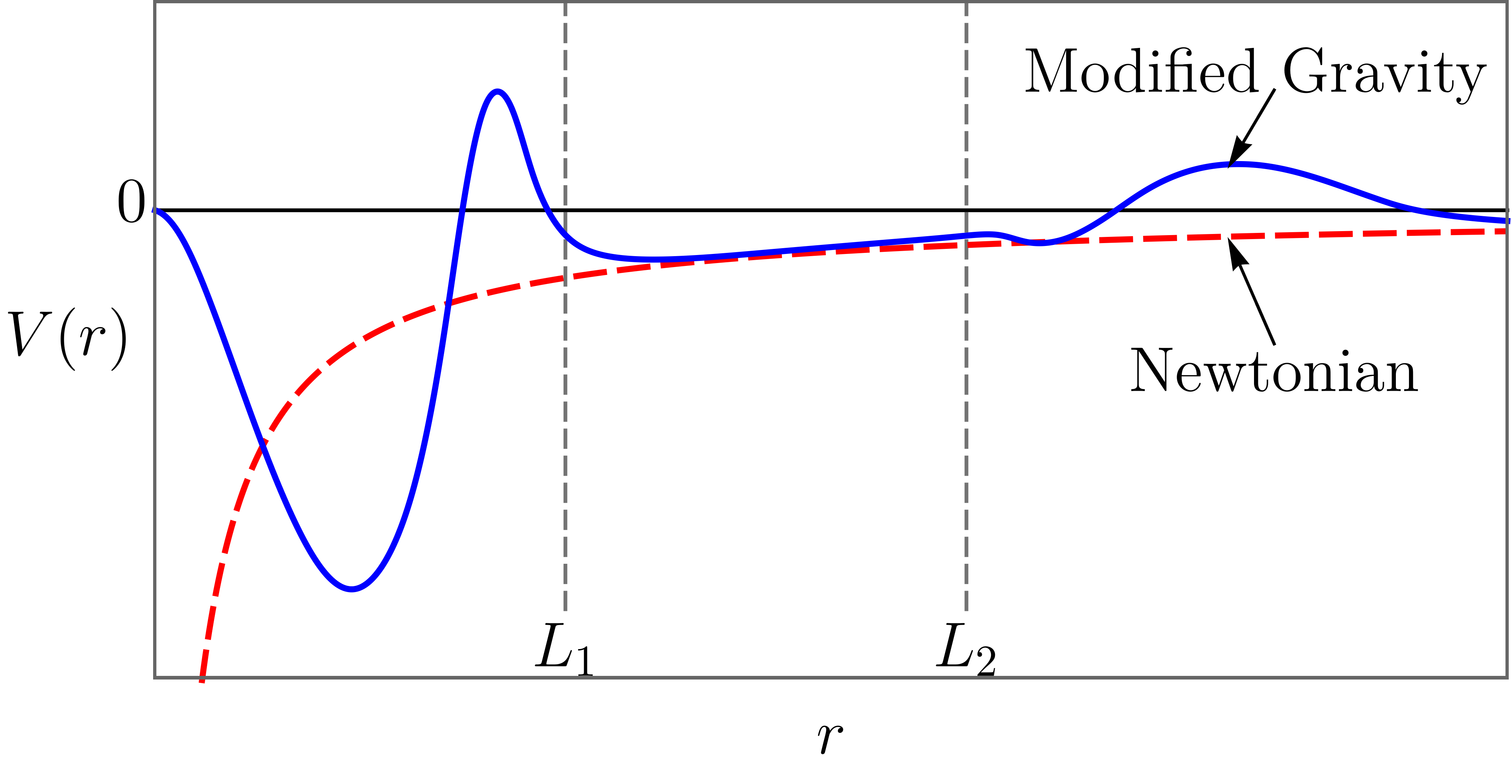
Now, a generic way of parametrizing departures from the standard gravitational realm is to factorize

where $F_{1}(r)$, $F_{2}(r)$ and $F_{3}(r)$ are three functions which can be chosen suitably to play specific roles as follows:

The function $F_{1}(r)$ can be chosen such that the singularity at $r=0$ gets smoothened. A suitable choice is

where $\alpha$ is a dimensionless positive constant, and $\ell_{1},\ell_{2}$ are positive constants of the dimension of length, either of which could be the Planck length, however, strictly speaking, they just need to be less than $L_{1}$.

The function $F_{2}(r)$, on the other hand, can make the gravitational potential $V(r)$ deviate further from the Newtonian one, outside the experimentally tested range $r\in(L_{1},L_{2})$, without the introduction of any zeroes however. A suitable choice for this may be, for instance,

where $r_{0l}$ and $r^{\prime}_{0l^{\prime}}$ are two sets of constants of dimension of length, $r_{0l}<L_{1}$ and $r^{\prime}_{0l^{\prime}}>L_{2}$ for all integer values of the indices $l$ and $l^{\prime}$ respectively, up to certain finite numbers, $s$ and $s^{\prime}$. Assuming, without loss of generality, $r_{0s}>r_{0(s-1)}>\dots>r_{01}$ and $r^{\prime}_{0s^{\prime}}>r^{\prime}_{0(s^{\prime}-1)}>\dots>r^{\prime}_{01}$, one can distinguish the nature of $V(r)$ at short and long distances, respectively.

The function $F_{3}(r)$ can finally be chosen to incorporate zero(es) in $V(r)$. A suitable chosen form is

which encodes all the short-distance zeroes $r_{i}\ll L_{1}$ (say, $n$ in number) and all the long-distance zeroes $r^{\prime}_{j}\gg L_{2}$ (say, $n^{\prime}$ in number), with respective integer multiplicities $\nu_{i}$ and $\nu^{\prime}_{j}$, under the assumption $r_{n}<r_{n-1}<\dots<r_{1}$ and $r^{\prime}_{1}<r^{\prime}_{2}<\dots<r^{\prime}_{n^{\prime}}$, without loss of generality.

In the remainder of this paper, we shall stipulate the constants $\ell_{1}=\ell_{2}=0$, as well as assume $r_{0l}\to 0$ and $r^{\prime}_{0l^{\prime}}\to\infty$, whence $F_{1}(r)=F_{2}(r)=1$, i.e., the full function $F(r)=F_{3}(r)$ given by Eq. (5). Moreover, we shall set $n=n^{\prime}=\nu_{1}=\nu_{1}^{\prime}=1$ in Eq. (5), since as explained below in section V, a single pair of short and long distance simple zeroes (i.e., the zeroes of unit multiplicity) is necessary and sufficient for a non-singular cyclic universe.

Given the modified Newtonian potential $V(r)$, Eq. (1), as our starting point, it is convenient to resort to a quasi-Newtonian (QN) cosmological formulation, following standard texts [8, 9, 10]. In particular, we take the specific approach of ref. [11], applicable to the standard form of the gravitational potential except with a varying Newtonian coupling $G_{\text{\scriptsize eff}}(r)$. This is tenable since we can always recast Eq. (1) in such a form with $G_{\text{\scriptsize eff}}(r)=GF(r)$.

With $F(r)=F_{3}(r)$, alongside $n=n^{\prime}=\nu_{1}=\nu_{1}^{\prime}=1$ in Eq. (5), the QN approach yields the following dynamical equation for a system of $N$ perfect fluids (presumably non-interacting):

where $\,a=a(t)=r(t)/\ell_{0}$ (with $\ell_{0}$ a fiducial length) is the cosmological scale factor, $H=H(t)=\dot{a}(t)/a(t)$ (with the dot $\{\cdot\}\equiv d/dt$) is the QN analogue of the Hubble parameter, $a_{1}$ and $a_{1}^{\prime}$ are the small and large values of $a$ at which $H$ vanishes, i.e., the early bounce and future turnaround points in the course of evolution of the Universe respectively, $\rho_{{}_{I0}}$ are the energy densities of the individual fluid species at the present epoch ($t=t_{0}$), $\mathsf{w}_{{}_{I}}$ are the corresponding equation-of-state (EoS) parameters (considered to be constants, for brevity), and $k$ is a dimensionless constant proportional to the total energy of the system per unit mass, $E$ (see the Appendix A for all the details). Thus, $k=0$ when $E=0$, and furthermore, one can always set $k=\pm 1$ for $E\lessgtr 1$, irrespective of stipulating the scale factor $a=1$ at the present epoch ($t=t_{0}$) without loss of generality. Hence, from a purely mathematical standpoint, Eq. (6) can be interpreted as the QN analogue of the Friedmann equation in standard cosmology, with the last term in the former resembling the spatial curvature term appearing in the latter.

In fact, Eq. (6) may rather appropriately be referred to as the modified Friedmann equation (MFE), arising from the modified Newtonian potential $V(r)$. Note also that the QN approach, although quite heuristic, generically leads to cosmological evolution equations same in mathematical form as those describing the cosmic background level dynamics in the standard framework [11]. This is irrespective of the component fluid/field configuration, even when many such components are relativistic per se. Therefore, notwithstanding the QN origin, Eq. (6) can safely be taken as the governing equation in a cosmological analysis concerning the background evolution. On the other hand, the analysis that inherently refers to the cosmological perturbations would require a relativistic (covariant) embedding of the modified Newtonian potential. This, despite being a hard proposition, is shown to be achievable in some of our works — the preceding ones [11, 12], and that currently underway [13] — see the discussions in the concluding part of this paper.

For simplicity, we consider only the known forms of fluid components, viz., radiation, non-relativistic pressureless matter (dust) and a cosmological constant $\Lambda$, with the respective energy densities $\rho_{r0}$, $\rho_{m0}$ and $\rho_{\Lambda 0}$ at the present epoch ($t=t_{0}$ or $a=1$), and EoS parameters $\mathsf{w}_{r}=1/3$, $\mathsf{w}_{m}=0$ and $\mathsf{w}_{\Lambda}=-1$. Defining, in the usual way, the corresponding density parameters, as well as that for the $k$-contributor, at $t=t_{0}$:

with $\rho_{c0}=3c^{2}H_{0}^{2}/(8\pi G)$ the critical density at $t=t_{0}$, and $H_{0}\equiv H|_{t=t_{0}}$ the Hubble’s constant, we express Eq. (6) rather conveniently as

Evaluating this at $t=t_{0}$ (or $a=1$) we get the constraint

using which we eliminate $\Omega_{\Lambda 0}$ from Eq. (8) to write

Check that for $a_{1}=0$ and $a_{1}^{\prime}\to\infty$, Eqs. (8), (9) and (10) reduce to the respective ones for the $\Lambda$CDM model in presence of radiation and the $k$-term. However, given the minuscule abundance of the Cosmic Microwave Background (CMB) radiation in the observed Universe at present, we shall ignore the contribution of $\Omega_{r0}$ in what follows. Furthermore, we shall set $\Omega_{k0}=0$, in view of the gross observational support for the spatial flatness in the standard cosmological paradigm.

With $\Omega_{r0}=0=\Omega_{k0}$, Eq. (10) reduces to the following form, in terms of the redshift $z=a^{-1}-1\,$:

In order to confront this with observational data, we carry out a statistical maximum likelihood analysis for the parameters concerned, using the standard Markov-chain Monte Carlo (MCMC) technique.

The datasets we consider are from three low-$z$ observations and two high-$z$ ones. The low-$z$ data include $51$ direct measurements of $H(z)$ using (primarily) the Cosmic Chronometers (CC) [14, 15], $1701$ datapoints from the Pantheon⁺ Supernovae type-Ia (SNIa) distance-redshift measurements [16], and $15$ datapoints from the baryon acoustic oscillation (BAO) distance measurements [17, 18, 19]. The high-$z$ data, on the other hand, comprise of the compressed Planck 2018 CMB distance-prior likelihood ($4$ points) [20], and the primordial light-element abundance constraints ($2$ points) from big bang nucleosynthesis (BBN) [21, 22, 23] — see the Appendix B for more details. As explained therein, a joint analysis with all these data amounts to minimizing the total negative log-likelihood, or $\chi^{2}_{\rm tot}$, with respect to the parameters concerned.

The parameter vector for our cyclic scenario is

where, apart from $H_{0}$ and $\Omega_{m0}$, we have the nuisance parameter $\Delta M$ denoting the absolute-magnitude offset of the Pantheon⁺ SNIa sample, the comoving sound horizon at the baryon drag epoch, $r_{d}$, the physical baryon density at the present epoch, $\omega_{b}$, and the bounce and turnaround scale factor ten-folds, $N_{1}\equiv\log_{10}a_{1}$ and $N_{1}^{\prime}\equiv\log_{10}a_{1}^{\prime}$, respectively. For $\Lambda$CDM, which we consider as a reference model to compare with, all the parameters except $N_{1}$ and $N_{1}^{\prime}$ in Eq. (12) are of relevance. The total number of parameters, $N_{\rm par}$, is therefore, five for $\Lambda$CDM, compared to the seven in the cyclic scenario.

Fig. 2 shows the one- and two-dimensional posterior distributions (up to $2\sigma$) for the cyclic scenario as well as for $\Lambda$CDM, obtained using the Goodman-Weare affine-invariant ensemble sampler emcee for MCMC [24], with flat priors listed in Table 1, alongside the estimated parameter values (best fits and the $1\sigma$ or $68\%$ confidence limits). The convergence is assessed by the well-known Gelman-Rubin statistic [25], with the associated tolerance factor found to be ${\widehat{R}}=1.011$ for the cyclic scenario and ${\widehat{R}}=1.0025$ for $\Lambda$CDM. While the former is well within the range $(1.01,1.05)$ categorized ‘good’, the latter is ‘excellent’ ($<1.01$).

The estimated best fit $N_{1}=-13.2296$ and the best fit $N_{1}^{\prime}=0.4703$ in Table 1 correspond to the scale factor values $a_{1}=5.8939\times 10^{-14}$ and $a_{1}^{\prime}=2.9532$ respectively. While the later suggests a future turnaround from an expanding to a contracting phase of cosmic evolution when the Universe grows to about thrice as much its present size, the former shows that the bounce in the past, from a contracting to the expanding phase, occurs when the Universe is extremely minute in size. In fact, such a low value of $a_{1}$ implies that the bounce happens well before the epoch at which cosmological perturbations associated with the observed CMB anisotropies enter the horizon, or in other words, all the observable CMB modes remain super-horizon during the bounce. Hence, we may safely infer that the cosmic background evolution due to the MFE keep the CMB power spectrum unaffected and the cyclic scenario consistent with the Planck CMB observations. Also, the bounce is far upstream of the primordial nucleosynthesis which typically occurs around $a\sim 10^{-10}$. So the MFE modification to the standard form of the early expansion history of the Universe during the BBN era, till the recombination, is practically negligible. As such, the standard pre-recombination or BBN microphysics, including the sound horizon and the physics encoded in the compressed Planck likelihood remain unchanged, thus ensuring the compliance of the cyclic scenario with the BBN constraints as well.

Table 1 also quotes a higher best fit value of the Hubble constant $H_{0}$ for the cyclic scenario than for $\Lambda$CDM, $71.0267$ to $69.1491$. This may be considered as a positive outcome since in a joint analysis of any given model, using data from both low-$z$ and high-$z$ observations, an $H_{0}$ estimate higher than its $\Lambda$CDM value is often desired for a potential resolution of the Hubble tension (see for e.g. [26] and references therein). While no claim for the complete aversion of the discrepancy amounting to such a tension can be made as such for the cyclic scenario, we may say that the latter at least opens a phenomenological avenue for alleviating the persistent problem. In fact, this is corroborated by another desirable outcome — the lowered best fit of $r_{d}$, the sound horizon at the photon-drag epoch, for the cyclic scenario than for $\Lambda$CDM, $144.763$ to $147.537$ in Table 1.

On the whole, in spite of having two additional parameters, the cyclic scenario provides a better fit to the combined data than $\Lambda$CDM. This is shown by the corresponding statistics summarized in Table 2, viz., the minimized $\chi^{2}_{\rm tot}$ which is denoted by $\chi^{2}_{\rm min}$, the goodness of fit $\chi^{2}_{\rm dof}$ which is the $\chi^{2}_{\rm min}$ per degree of freedom (dof), the Akaike and Bayesian information criteria, AIC and BIC, and the Bayes factor $\ln\mathcal{Z}$ (see the Appendix B for definitions). There are significant reductions in the $\chi^{2}_{\rm min}$, $\chi^{2}_{\rm dof}$, AIC and BIC values, and a substantial enhancement in $\ln\mathcal{Z}$, for the cyclic scenario than those for $\Lambda$CDM — all of which imply better fitting of the former with the data compared to the latter. In particular, the changes $\Delta$AIC $=-27.29$ and $\Delta$BIC $=-16.33$ are significant enough to favor the cyclic scenario over $\Lambda$CDM comprehensively. A fairly large Bayes factor $\Delta\ln\mathcal{Z}=13.3$, computed via nested sampling [27], supports this further, and in fact shows a strong evidence in favor of the cyclic scenario on the Jeffreys’ scale [28].

Recall the MFE (6) above, or more specifically Eq. (8), describing the cyclic evolution for the minimal setting $n=n^{\prime}=\nu_{1}=\nu_{1}^{\prime}=1$ in Eq. (5). Such a setting is in fact quite distinct, rather than a simplifying one. To see this, note first that Eq. (5), and consequently the cosmological equation (22) in the Appendix A, imply the following generalized form of Eq. (8):

assuming $\Omega_{r0}=0=\Omega_{k0}$. Consider next, a particular bounce point $a=a_{b}$, which is a zero of multiplicity $\nu$, say. In a close neighborhood (say, $\varepsilon$) of $a_{b}$, one has $\dot{a}\propto(a-a_{b})^{\nu/2}$. So the traversal time from $a_{b}$ to $a_{b}+\varepsilon$, i.e., $\Delta t\propto\int_{a_{b}}^{a_{b}+\varepsilon}da\left(a-a_{b}\right)^{-\nu/2}\,,$ converges only for $\nu=1$. Similar argument holds in the vicinity of a particular turnaround $a=a_{t}$ as well. Thus, simple zeroes, i.e., the zeroes of multiplicity $\nu=1$, are necessary, and for any $\nu\geq 2$ the bounce (turnaround) degenerates into an asymptotically static state approached over infinite cosmic time — the emergent (loitering) universe limit — and the cyclicity is lost. Moreover, since $H^{2}>0$ throughout, in the interval between a given bounce $a_{b}$ and a given turnaround $a_{t}$, the cosmic evolution oscillates indefinitely, thus forming multiple cycles. Nevertheless, our predictions on the past or(and) future are based on what we see in our present observable universe, at $t=t_{0}$ or $a=1$. Therefore, limiting our attention to one zero on each side of $a=1$, pertaining to a single cycle, is sufficient. All other cycles are mere replica of this cycle, which we label for convenience as ‘$1$’. This means that the corresponding bounce-turnaround pair $(a_{1},a_{1}^{\prime})$, together with the measured density parameters, determines the evolving scale factor, $a(t)$, at all times.

In the integral form Eq. (8) is expressed as

With $\Omega_{r0}=0=\Omega_{k0}$, and $\Omega_{\Lambda 0}$ eliminated via the constraint (9), we work out the integral numerically by using the estimated values of $\Omega_{m0}$, $a_{1}$ and $a_{1}^{\prime}$, to obtain $H_{0}(t-t_{0})$ as a function of the scale factor $a$ in the cyclic scenario. Similar functional variation is found for $\Lambda$CDM, by setting $a_{1}=0,a_{1}^{\prime}\to\infty$ and using the corresponding estimate of $\Omega_{m0}$. Inverting these we determine the time-evolution of the scale factor, $a(t)$, and consequently that of the Hubble parameter, $H(t)$, in either cases.

While the evolution of $a(t)$ with the dimensionless time variable $H_{0}t$ (or $t/t_{H}$, where $t_{H}=H_{0}^{-1}$ is the Hubble time) is shown in the top panel of Fig. 3, that of the reduced Hubble parameter $H(t)/H_{0}$ with $H_{0}t$ is shown in the top panel of Fig. 4. In each of these figures, the evolution before and after the bounce are depicted by the cycles on the left and right respectively, and the contracting and expanding phases, the present epoch and the bounce and turnaround points are duly marked. In fact, the value of the scale factor at the bounce, $a=a_{1}$ (taken to be its estimated best fit, $5.8939\times 10^{-14}$ in Table 1), is enhanced by a factor of $10^{12}$ in order to make the illustration clear. Moreover, exaggerations near $a=a_{1}$ and near $a=1$ are shown, respectively, in the bottom panels (A) and (B) of Fig. 3 and of Fig. 4 for further clarity.

Right after the bounce, the cyclic evolution begins to track the $\Lambda$CDM one, but slowly drifts away as time progresses. The drift remains quite insignificant however, implying that the tracking continues even at the present epoch $t=t_{0}$, and afterwards till a cosmic time $t\simeq 14\,H_{0}^{-1}$ or so. Of course, the value of $t_{0}$, and hence the present age of the Universe, differs in the cyclic and $\Lambda$CDM cases. While for $\Lambda$CDM, the estimated best fit values of the associated parameters listed in Table 1 show that the present age of the Universe (since the big bang) is $0.9713\,H_{0}^{-1}|_{\Lambda{\rm CDM}}=13.7440\,{\rm Gyr}\,,$ for the cyclic Universe, the associated best fit parametric estimates show that the present age (since the bounce) is $1.0651\,H_{0}^{-1}|_{\rm Cycl}=14.6727\,{\rm Gyr}\,.$ The same estimates also indicate that the next turnaround is at $29.8165\,{\rm Gyr}$ from the present epoch, and the full cosmic cycle has a period of $88.9784\,{\rm Gyr}$.

It is worth emphasizing that Eqs. (6)–(8) cannot simply be regarded as those of another bouncing cosmological model expanding the literature on the subject. They actually describe a class of cosmologies governed by a generalized form of the Friedmann equation given by

where $\rho(a)$ is the energy density of the total fluid content of the Universe, and the function $g(a)$ collects whatever microphysical or gravitational corrections the underlying theory provides. The total fluid content may in general be due to several components. For $N$ such components with energy densities $\rho_{{}_{I0}}$ at the present epoch, and (presumably constant) EoS parameters $\mathsf{w}_{{}_{I}}$, the expression for $\rho(a)$ is that given by Eq. (23) in the Appendix A.

A non-singular bounce at $a=a_{b}$ and a subsequent turnaround at $a=a_{t}$ occur where $H=0$ and $\dot{H}\,>\,0$ and $<\,0$ respectively, i.e., where $g(a)$ has positive real zeroes at a small value of $a$ and at a large value of $a$, respectively. A natural form of $g(a)$ in terms of its short-distance roots $a_{i}$ (corresponding to $r_{i}\ll L_{1}$) and large-distance roots $a_{j}^{\prime}$ (corresponding to $r_{j}^{\prime}\gg L_{2}$) is the factorized structure of Eq. (13), i.e.,

with $\nu_{i}$ and $\nu_{j}^{\prime}$ denoting the multiplicities of the zeroes. Specific bounce and cyclic scenarios differ only in the characterization of which $g(a)$ their dynamics generate. Therefore, all such scenarios live inside the family parametrized by $(\{\rho_{{}_{I0}}\},\{\mathsf{w}_{{}_{I}}\},\{a_{i}\},\{a_{j}^{\prime}\},\{\nu_{i}\},\{\nu_{j}^{\prime}\})$ [29]. Within this family, finite-time cyclicity selects the simple zeroes uniquely, and the innermost zeroes at each end of a given cycle controls the entire accessible evolution. The minimal choice $n=n^{\prime}=\nu_{1}=\nu_{1}^{\prime}=1$ is therefore not a simplifying assumption but the observationally sufficient representative of the whole class.

Let us cite a few examples:

Across these examples, one can see that the model-dependent physics enters in Eq. (15) only through the specification of the location, number, and order of the zeroes of the modulating function $g(a)$. With $g(a)$ given by Eq. (16), it is evident that Eq. (15) is characteristically equivalent to the Fridmann equation describing a unified, model-independent parametrization of not just the bouncing, but cyclic cosmologies as well, where $\{a_{i}\}$ and $\{a_{j}^{\prime}\}$ are the phenomenological parameters to be confronted with the observational data.

Let us conclude with a discussion on the following:

References

- [1] C.D. Hoyle et al., Phys. Rev. D 70 (2004) 042004.
- [2] D.J. Kapner et al., Phys. Rev. Lett. 98 (2007) 021101.
- [3] E.G. Adelberger, J.H. Gundlach, B.R. Heckel, S. Hoedl and S. Schlamminger, Prog. Part. Nucl. Phys. 62 (2009) 102.
- [4] T. Westphal, H. Hepach, J. Pfaff and M. Aspelmeyer, Nature 591 (2021) 225.
- [5] B. Bertotti, L. Iess, P. Tortora, Nature 425 (2003) 374–376.
- [6] C. Will, Liv. Rev. Rel. 17 (2014) 4.
- [7] N. Aghanim et al. (Planck Collaboration), Astron. Astrophys. 641 (2020) A6.
- [8] R. D’Inverno, Introducing Einstein’s Relativity, Clarendon Press, Oxford (1992).
- [9] S. Weinberg, Cosmology, Oxford (2008).
- [10] A. Liddle, An Introduction to Modern Cosmology, 2nd ed., Wiley (2003).
- [11] S. Das and S. Sur, Eur. Phys. J. Plus 139 (2024) 1049.
- [12] S. Das, M. Fridman and S. Sur, Phys. Rev. D 111 (2025) 6, 064047.
- [13] S. Sur, R. Kapoor and S. Das, in preparation.
- [14] M. Moresco et al., JCAP 05 (2016) 014.
- [15] R. Monjo, Astrophys. J. 967 (2024) 66.
- [16] D. Brout et al., Astrophys. J. 938 (2022) 110.
- [17] D.J. Eisenstein et al., Astrophys. J. 633 (2005) 560.
- [18] S. Alam et al. (eBOSS Collaboration), Phys. Rev. D 103 (2021) 083533.
- [19] A.G. Adame et al. (DESI Collaboration), JCAP 02 (2025) 021.
- [20] N. Arendse et al., Astron. Astrophys. 639 (2020) A57.
- [21] C. Pitrou, A. Coc, J.-P. Uzan, and E. Vangioni, Mon. Not. Roy. Astron. Soc. 502 (2021) 2474.
- [22] E. Aver, K.A. Olive and E.D. Skillman, JCAP 07 (2015) 011.
- [23] R.J. Cooke, M. Pettini, C.C. Steidel, Astrophys. J. 855 (2018) 102.
- [24] J. Goodman and J. Weare, Commun. Appl. Math. Comput. Sci. 5 (2010) 65.
- [25] A. Gelman and D.B. Rubin, Statistical Science 7 (1992) 457.
- [26] E. Di Valentino et al., Astron. Astrophys. Rev. 30 (2021) 2.
- [27] J. Skilling, Bayesian Anal. 1 (2006) 833.
- [28] H. Jeffreys, The Theory of Probability, 3rd ed., Oxford University Press, Oxford (1961).
- [29] R.H. Brandenberger and P. Peter, Found. Phys. 47 (2017) 797.
- [30] A. Ashtekar and P. Singh, Class. Quant. Grav. 28 (2011) 213001.
- [31] A. Ashtekar, T. Pawlowski and P. Singh, Phys. Rev. Lett. 96 (2006) 141301.
- [32] V. Taveras, Phys. Rev. D 78 (2008) 064072.
- [33] Yu. Shtanov and V. Sahni, Phys. Lett. B557 (2003) 1.
- [34] L. Randall and R. Sundrum, Phys. Rev. Lett. 83 (1999) 4690.
- [35] P. Binétruy, C. Deffayet and D. Langlois, Nucl. Phys. B 565 (2000) 269.
- [36] S. Nojiri and S. D. Odintsov, Phys. Rept. 505 (2011) 59.
- [37] A. De Felice and S. Tsujikawa, Liv. Rev. Rel. 13 (2010) 3.
- [38] S.M. Carroll, V. Duvvuri, M. Trodden and M.S. Turner, Phys. Rev. D 70 (2004) 043528.
- [39] Y.-F. Cai, Sci. China Phys. Mech. Astron. 57 (2014) 1414.
- [40] Y.-F. Cai, T. Qiu, Y.-S. Piao, M. Li and X. Zhang, JHEP 0710 (2007) 071.
- [41] Y.-F. Cai, E.N. Saridakis, M.R. Setare and J.-Q. Xia, Phys. Rept. 493 (2010) 1.
- [42] J. Khoury, B.A. Ovrut, P.J. Steinhardt and N. Turok, Phys. Rev. D 64 (2001) 123522.
- [43] P.J. Steinhardt and N. Turok, Science 296 (2002) 1436.
- [44] J.-L. Lehners, Phys. Rept. 465 (2008) 223.
- [45] E.I. Buchbinder, J. Khoury and B.A. Ovrut, Phys. Rev. D 76 (2007) 123503.
- [46] N. Arkani-Hamed, H.-C. Cheng, M.A. Luty and S. Mukohyama, JHEP 0405 (2004) 074.
- [47] H.-J. Blome, C. Chicone, F.W. Hehl and B. Mashhoon, Phys. Rev. D 81 (2010) 065020.
- [48] J. Tabatabaei, S. Baghram and B. Mashhoon, Mon. Not. Roy. Astron. Soc. 530 (2024) 795.
- [49] S. Das, M. Fridman, D. Kuniyal and S. Sur, work in progress.
- [50] R.C. Tolman, Relativity, Thermodynamics and Cosmology, Clarendon Press, Oxford (1934).
- [51] W. Hu and N. Sugiyama, Astrophys. J. 471 (1996) 542.