The driving mode of turbulence in disc galaxy simulations with adaptive mesh refinement
Abstract
Turbulence is a key ingredient in controlling the structure of the interstellar medium (ISM) and the formation of stars. However, we still lack a detailed understanding of the drivers of turbulence in the ISM of galaxies. Previous idealised simulations of turbulence employ a stochastic forcing field to drive turbulence. The geometry of this forcing field — whether it is predominantly solenoidal or compressive — is a key parameter governing how turbulence shapes the ISM density distribution and regulates the star formation rate. This is commonly expressed through the turbulence driving parameter (), which quantifies the relative contribution of compressive versus solenoidal driving. Therefore, an accurate knowledge of the driving parameter is essential for understanding and predicting star formation, and for sub-grid modelling of ISM physics and the star formation rate. In this work, we introduce an algorithm to measure the turbulence driving parameter in adaptive mesh refinement (AMR) simulations of galaxies on variable turbulence kernel sizes. We focus our analysis on a synthetic Large Mallenanic Cloud (LMC), present-day analogue with a total mass M⊙. We find that turbulence is driven primarily solenoidally () within the inner of the galaxy, and becomes increasingly compressive with towards the outskirts, . The volume-weighted median across the disc, , is consistent with the natural mixture of driving modes. We further find that is weakly correlated with the strength of shear, in that solenoidal driving tends to be associated with regions of higher shear, as expected for the more central parts of galaxies. These trends persist over Gyr of the galaxy’s evolution, and are largely insensitive to the choice of turbulence kernel size.
Keywords:
turbulence – hydrodynamics – methods: numerical – ISM: structure – galaxies: ISM1 Introduction
Turbulence in the interstellar medium (ISM) plays a central role in regulating the evolution of galaxies. The driving mechanism of turbulence is a key parameter in determining the density distribution of gas (Molina et al., 2012; Hopkins, 2013; Nolan et al., 2015), setting the phase fraction in the multiphase ISM (Seifried et al., 2011; Micic et al., 2012) and regulating star formation (Federrath and Klessen, 2012; Padoan et al., 2014; Mathew et al., 2023). A key diagnostic of the turbulent forcing is the turbulence driving parameter , defined by
| (1) |
where is the standard deviation of the ratio of density to the mean density and is the root-mean-square (rms) Mach number. The parameter has been used to quantify the relative contribution of solenoidal (divergence-free) and compressive (curl-free) driving modes in periodic-box simulations of stochastically driven turbulence in non-magnetized isothermal gas (Padoan et al., 1997; Passot and Vázquez-Semadeni, 1998a; Federrath et al., 2008; Federrath et al., 2010; Price and Federrath, 2010; Konstandin et al., 2012b, see), as well as magnetized isothermal and non-isothermal plasmas (Molina et al., 2012; Federrath and Banerjee, 2015; Nolan et al., 2015). Purely solenoidal driving, which can be thought of as turbulence driven by a divergence free stochastic forcing field, corresponds to , while purely compressive driving yields , with mixed driving producing intermediate values. The parameter is especially relevant for star formation studies as varying can change star formation rates by an order of magnitude (Federrath and Klessen, 2012; Salim et al., 2015; Federrath, 2018, see) and changes the characteristic mass of the IMF (Mathew et al., 2023).
Understanding the spatial variation of within galaxies and molecular clouds offers a unique window into the physical processes responsible for stirring the ISM and regulating star formation. Some work has been done in this direction, particularly focusing on measuring in selective regions of various galaxies. For instance, Ginsburg et al. (2013) measured the turbulence driving parameter of the system dubbed GRSMC 43.30-0.33, Federrath et al. (2016) looked at the central molecular zone cloud G0.253+0.016, Menon et al. (2021) measured turbulence driven by ionizing feedback in the pillars of the Carina Nebula, Sharda et al. (2022) measured the parameter of the star-forming region N159E in the Large Magellanic Cloud, Marchal and Miville-Deschênes (2021) looked at the driving of turbulence in the high latitude WNM of the Milky Way, Gerrard et al. (2023); Gerrard et al. (2024) have produced maps of the parameter using HI observations of the Small Magellanic Cloud and high latitude clouds in the Milky Way. Finally, Miller et al. (2026) is the only observational work so far that as studied in full-disc observations (in NCG1313 and NGC7793). The driving mechanism of turbulence has also been studied in controlled simulations of molecular clouds (Körtgen et al., 2017), idealized box simulations of the ISM (Seifried et al., 2011), and kpc-sized shearing boxes of galactic discs (Gerrard and Federrath, 2026). The only study of turbulence driving in full-scale galaxy simulations to date is that presented by Jin et al. (2017), however, resolution constraints did not allow them for a robust determination of . In the realm of numerical simulations more broadly, works like Federrath et al. (2011), Pan et al. (2016), and Grisdale et al. (2017) have quantified the fraction of kinetic energy in compressive vs. solenoidal motions in the gas. Similarly, such characterisation has been done in observations (Orkisz et al., 2017). However, the ratio of solenoidal to compressible modes in the velocity field is not a direct probe of the parameter relevant for determining star formation efficiency, ISM phase, and density distribution of the gas. In fact, even purely compressive driving induces solenoidal motions in the gas at a level as high as of the total kinetic energy (Federrath et al., 2010).
In this work, we extend the algorithm for measuring the parameter introduced in Gerrard et al. (2023) to adaptive-mesh refinement (AMR) simulations. We use it to study the driving of turbulence in a present-day Large Magellanic Cloud (LMC) analogue with an initial gas fraction of , created with the Nexus simulation framework (Tepper-García et al., 2024).
The rest of this paper is structured as follows: in Section 2, we briefly describe our galaxy simulations. Section 3 introduces the algorithm for calculating . Section 4 demonstrates how the driving parameter of turbulence varies across the simulated galaxy in terms of radius, scale height, and over time, and how it is correlated with shear. Finally, we summarise our results in Section 5.
2 Galaxy simulation
The main goal of this work is to study the driving of turbulence over galactic scales, rather than just for individual clouds. We choose to do so using a system that resembles today’s LMC. Thus, we focus our attention on a single galaxy model, and defer a comparative analysis of different galaxy models to future work.
2.1 Initial conditions
We use one simulation of the suite introduced by and Bland-Hawthorn et al. (2024, see also ). Specifically, we adopt the high-resolution version of synthetic galaxy dubbed ‘fd50_fg00_nac’, a multi-component system with a dark matter (DM) halo mass of M⊙, a total disc mass of M⊙, of which 20% is initially in the form of gas (see Bland-Hawthorn et al., 2024, tab. 1).
The galaxy models are constructed and evolved with the Nexus framework (Tepper-García et al., 2024). Particle positions and velocities of each of the components making up the galaxy are generated with the self-consistent modelling module (SCM) provided by the Action-based GAlaxy Modelling Architecture (agama) stellar dynamical library (Vasiliev, 2019), which has been complemented to treat gas in addition to the DM and stellar components. The DM halo virial radius and scale radius are kpc, and kpc, respectively. The total mass and structural parameters of the halo are broadly consistent with today’s LMC (Vasiliev et al., 2021, e.g.).11 1 This galaxy model is also broadly consistent with a Milky-Way progenitor at (Bland-Hawthorn and Gerhard, 2016, see also Bland-Hawthorn et al. 2024). The pre-assembled stellar disc and the gas disc both have an initial scale length kpc. The initial scale height of the stellar disc is roughly kpc; the initial scale height of the gas disc is roughly less than that at the centre, and increases with radius (‘flaring’ disc). It is worth mentioning though that its initial value is irrelevant, as the disc structure necessarily (and significantly) changes once the disc is allowed to undergo cooling and heating, and to form stars.
The initial conditions are evolved with the adaptive mesh refinement (AMR), -body/hydrodynamical code Ramses (Teyssier, 2002), augmented with the galaxy formation physics (incl. star formation and feedback processes) outline in Agertz et al. (2013) and Agertz et al. (2021), see Bland-Hawthorn et al. (2024) for more details on the specific setup in this work.
The DM halo, pre-assembled stellar disc, and gas disc, are sampled, respectively, with , , and particles. The latter number is only relevant for the construction of the initial conditions – at runtime, the gas particles are mapped onto the computational grid of Ramses, resulting in cells, which changes during the evolution of the system as a consequence of the adaptive nature of the grid (see below). The composite system is evolved in a cubic simulation volume with a length of 100 kpc per side. The total simulation timespan is about 2 Gyr. At runtime, the AMR grid is maximally refined up to level 14, implying a limiting spatial resolution of 100 kpc / pc.22 2 Note that this marginally resolves the scale height of the gas disc close to the centre at initialisation. However, as explained above, it is irrelevant since the disc 1) has a larger scale height away from the centre, and 2) will thicken quickly and significantly at runtime as a result of stellar feedback. To allow the gas disc to settle, we evolve the system with an adiabatic equation of state (, appropriate for a monoatomic gas) for 80 Myr, after which cooling/heating, star formation and feedback are ‘switched on’. We refer the reader to Tepper-García et al. (2024) for further details about the initial conditions and the simulation techniques – and, in particular, Bland-Hawthorn et al. (2024); Bland-Hawthorn et al. (2025) for the galaxy formation module.
2.2 Galaxy properties and morphology
Figure 1 shows the state of the gas at the end of the simulation ( Gyr). The top and bottom panels in the left column show the projection of the gas density along the - and -axes, respectively. The galaxy has developed sub-structures and flocculent spiral arms. The top panel in the middle column displays the density-weighted value of the gas’ vertical velocity projected along the -axis; and similar for the component in the bottom panel. In this projection, the disc’s rotation is discernible (blue-/redshift). The right column displays the density-weighted projection of the temperature along the -axis (top) and the -axis (bottom). As a result of stellar feedback, and the interplay between cooling and heating, the gas disc features diffuse pockets of hot material entrained within dense filamentary knots close to the plane, and plumes of gas ejected from the plane.

3 Turbulence analysis method
Equation (1) is based on idealised simulations of driven turbulence where the velocity and density fluctuations are induced entirely by turbulent motions. However, in real galaxies, the density and velocity distributions contain large-scale, systematic features and flows that originate from the inherent structure of a galaxy, such as large-scale rotation, gravitational gradients, etc. Not all of these motions and structures are turbulent. Therefore, in order to isolate the turbulent fluctuations, large-scale, systematic features must be subtracted before flow variables can be used for calculating (Federrath et al., 2016; Stewart and Federrath, 2022; Narayan et al., 2025). Here, we explain our algorithm for extracting the turbulent components of the flow from the synthetic galaxy’s ISM, with the ultimate goal of calculating .
3.1 Roving and smoothing kernel
Consider a set of all the cell-centred coordinates in an AMR-based galaxy simulation. Suppose is the collection of points in that satisfy some criteria set on the flow variables, for instance, a temperature criterion to restrict the analysis to just one gas phase, say the warm neutral medium. We define the functions
| (2) | ||||
| (3) |
where , and are the widths of the cells. Suppose we want to calculate the turbulence driving parameter at . Then, we define a roving kernel centred at as
| (4) |
where is the Euclidean norm defined by . The roving kernel is a Gaussian of full width at half maximum , truncated at a radius of times that FWHM (i.e. at ), so that . Throughout this work we adopt , and hence ; this choice is justified in Appendix A.
For , define a smoothing kernel centred at as
| (5) |
Note that the extent of the smoothing kernel is set by the cell size at the centre of the roving kernel, , rather than by that of the cell at which the smoothing is evaluated. A single smoothing scale is therefore applied uniformly across , so that the background subtracted at every point of a given roving kernel is defined with respect to the same physical length scale. Consequently, the smooth component depends on both and , as reflected in the notation below. Suppose is a flow variable. Then, we can calculate the Gaussian weighted mean of over a kernel centred at as
| (6) |
where . For , we define the smooth background component of at for the kernel centred at as
| (7) |
where , i.e. the smoothing kernel has half the FWHM of the roving kernel. Then, the turbulent component of at point for the kernel centred at is given by
| (8) |
3.2 Density dispersion and Mach number
We now describe the procedure for calculating and . We need to subtract the large-scale density structures and bulk velocities. We note that Gerrard et al. (2023) perform this subtraction on the line-of-sight velocity component and the logarithm of density (). The reason behind this seemingly odd choice of is that while turbulent velocity fluctuations are additive, turbulent density fluctuations are multiplicative (Vazquez-Semadeni, 1994, see), making the natural variable for obtaining the turbulent component.
For , we define
| (9) |
and, for each velocity component ,
| (10) |
Then, for , we define
| (11) |
| (12) |
with the dispersion of each component given by
| (13) |
In both cases , i.e. the moments are taken with the same Gaussian weight that defines the roving kernel. The turbulence driving parameter is then calculated as per Eq. (1), for point ,
| (14) |
Following Sharda et al. (2022), we reject results for any if has 30 or fewer cells.
3.3 Choice of , , and
While the notation looks complicated, the crux of the algorithm is similar to that of Gerrard et al. (2023) and Miller et al. (2026), who have also shown that the measurement of is largely independent of the kernel size, as long as the kernel size is not varied by factors of several, in which case the turbulence on a different kernel scale is probed. The relative insensitivity of with respect to changes in the kernel size arises because, while both and are strongly scale-dependent, the ratio of the two, i.e., , is only weakly dependent on kernel size (see Appendix A). Therefore, we choose , so as to have a sufficiently large number of cells in each kernel, while at the same time keeping it as small as possible to allow for an exploration of the spatial variation of the turbulence quantities across the galaxy.
We construct a roving kernel () around a cell () in the simulation data. As defined above, its FWHM is , i.e. times the diagonal of the cell , and it is truncated at FWHM (), giving . Note that the size of the roving kernel is adaptive unlike in Gerrard et al. (2023) and Miller et al. (2026), to account for the AMR nature of our datasets.
Eq. (7) evaluates the smooth background of a flow variable at every cell of the roving kernel, by convolving with a second Gaussian — the smoothing kernel — of FWHM with , i.e. half the FWHM of the roving kernel. The smoothing kernel is likewise truncated at . Defining it using Eq. (6) has the advantage of the volume weighting taking into account the AMR nature of the kernel and the normalization, allowing for gaps in the kernel in case some cells do not satisfy the physical criteria (like the choice of the ISM phase) used for constructing . Eq. (8) calculates the turbulent component of the flow by subtracting the Gauss-smoothed background. This procedure removes all flow features that appear at length scales greater than half the size of the roving kernel. The turbulent Mach number and the density dispersion are calculated over a roving kernel with the same Gauss weighting as in Eq. (6).
3.4 Choice of ISM phase
The ISM is composed of multiple thermally distinct phases. The molecular phase consists predominantly of molecular hydrogen () and is generally the coldest and densest phase, with typical temperatures of . The cold neutral medium (CNM) consists of dense, atomic gas and is typically characterized by . The warm neutral medium (WNM) is more diffuse and typically lies in the range . The unstable neutral medium (UNM) occupies an intermediate regime of between the CNM and WNM, where gas is thermally unstable to perturbations and can evolve towards either the cold or warm phase depending on local heating and cooling conditions. At higher temperatures () are the warm ionized medium (WIM) and the hot ionized medium (HIM), usually found in supernova-heated cavities.
The multi-phase nature of the ISM can significantly increase the density dispersion. This can lead to an overestimate of the turbulent density dispersion, as multiple phases can coexist without significant motions between the phases (Mohapatra et al., 2022). Furthermore, Eq. (1) is based on studies of isothermal turbulence. The Mach number, which depends on the sound speed, is therefore also affected by changes in the temperature, and the presence of different phases would consequently affect the turbulent Mach number. Therefore, as in Gerrard et al. (2023), we restrict our analysis to a narrow temperature range and study turbulence only in the WNM.
3.5 Example of a single kernel
We now demonstrate the action of the algorithm on a single kernel for calculating at a point inside the galactic disc. We choose a WNM cell in the galaxy, close to the centre. Figure 2 shows a single roving kernel (as defined in Eq. (4)) drawn around this cell. The kernel has a total radius of (corresponding to 3 radius of the corresponding Gaussian and spanning ), where , and are the cell sizes. The characteristic size of the kernel is set by the standard deviation of this Gaussian, . The top-left panels show a snapshot of the logarithm of the normalized density , in accordance with Eq. (6). The top-middle panel shows the smooth component of calculated using Eq. (7). The smoothing was performed using a Gaussian with a FWHM half the size of the Gaussian corresponding to the roving kernel. One can see that small-scale features have been smoothed out yielding a map of the density structure originating from non-turbulent sources. The top-right panel shows the turbulent component calculated using Eq. (8). The bottom three panels demonstrate the same procedure for the -component of the velocity.

The results of Figure 2 can be understood more quantitatively by looking at the statistics of the density and the velocity. In isothermal turbulence, the density approximately follows a log-normal distribution (Vazquez-Semadeni, 1994; Passot and Vázquez-Semadeni, 1998b), i.e., is Gaussian, and the velocity components follow a normal distribution (Federrath, 2013, e.g.,). Figure 3 shows a comparison between the density and the velocity statistics before and after background removal. The original data (left panels of Figure 3) have strong non-Gaussian components originating from large-scale structures and flows in the galactic disk. Background removal yields a density distribution close to a log-normal distribution and a nearly Gaussian velocity distribution (more specifically, the velocity components are Gaussian) for the major fraction (more than ) of the PDFs, both of which are strong signatures of turbulent motion (Kritsuk et al., 2007; Federrath et al., 2010; Federrath, 2013). The tails of the distributions deviate from the perfect log-normal and Gaussian distributions, which may be attributed to intermittency effects (She and Leveque, 1994; Kritsuk et al., 2007; Federrath et al., 2010; Konstandin et al., 2012a; Hopkins, 2013, see) as well as imperfect isolation of turbulent motions. However, these outliers constitute less than of the data and do not have a significant impact on the final measurements, i.e., the dispersions.
4 Results
In this section, we study the turbulence driving parameter in the WNM and determine its variation across the entire galactic disk. Figure 4 maps out the WNM in our galaxy snapshot, in order to focus on a single gas phase, required to robustly apply Eq. (1) – cf. Sec. 3.4. While selection of the WNM phase obviously removes some of the gas, it still covers a substantial fraction of the galactic disc, allowing us to study the turbulence across the entire disc.

4.1 Variation across the galaxy
Figure 5 shows volume-weighted projections of the density dispersion, Mach number, and driving parameter, while Figure 6 presents their probability distributions. These quantities are highly variable across the galaxy, however, clear trends emerge: the Mach number increases towards the galactic centre, while the turbulence driving parameter decreases, indicating that the turbulence driving becomes increasingly solenoidal towards the galactic centre. In particular, the driving becomes predominantly solenoidal () within the inner of the galaxy. In contrast, all three quantities remain largely unchanged along the vertical direction. The Mach number spans –, placing most of the gas in the transonic regime, as expected for the WNM (McClure-Griffiths et al., 2023; Gerrard et al., 2023, see also).
The high variability of the turbulence driving parameter may be the result of the local conditions and superposition of different driving mechanisms, such as supernova explosions, shear, etc. The map of in Figure 7 reinforces this picture: although the driving mode changes significantly from place to place, there is a systematic radial trend towards more compressive driving at larger galactocentric radii. Vertically, however, remains nearly constant. The left panel shows a roughly linear increase of with radius, well described by , whereas the right panel shows little variation along the -axis, the fitted slope of being consistent with zero, with an average value of . Both the level of small-scale variability and the systematic radial increase of are consistent with the observational findings of Miller et al. (2026) in NCG1313 and NGC7793.

4.2 Time evolution and correlation with shear
Solenoidal driving is often attributed to shearing motions (Federrath et al., 2016). In a galaxy, these can arise from differential rotation. In order to quantify shear, we use the norm of the traceless symmetric part of the shear tensor. The shear tensor () for a fluid is defined as
| (15) |
where is the th component of the velocity. The traceless symmetric part of the shear tensor () is given by
| (16) |
where is the Kronecker delta tensor. The norm of is defined by
| (17) |
For a consistent comparison, we Gaussian-average the norm of over the same length scales as the turbulent Mach number and the density dispersion. More rigorously, for the set of all cells in our simulation, and the set of all WNM points, we define
| (18) |
where and . The average value of is then given by , where (see Eq. 6).
We plot the average shear profile and the profile at four different times (, and Gyr) in Figure 8. The profiles are largely identical at different times during the galaxy evolution. The shear increases as one moves closer towards the galactic centre due to an increase in the strength of differential rotation. This is accompanied by a decrease in the turbulence driving parameter , i.e., towards more solenoidal driving. We also perform a cell-by-cell comparison of shear with in Figure 9. The inset on the top right shows the volume-weighted Spearman rank correlation coefficient (), which ranges from to across the four epochs. There is a weak, but significant anti-correlation between shear and and it is the tail of the distribution (corresponding to low ) that has a stronger anti-correlation with shear. This confirms that solenoidal driving is associated with high-shear environments. The lack of correlation for higher values of can be attributed to other local drivers of turbulence, like, supernovae.

5 Conclusions
Much of our quantitative understanding of astrophysical turbulence rests on idealised, periodic-box simulations in which turbulence is sustained by a stochastic forcing field of prescribed geometry. The turbulence driving parameter is the quantity that connects those controlled experiments to real, inhomogeneous systems, since it sets the width of the density PDF and thereby the star formation rate (Federrath and Klessen, 2012). In this work we have built that bridge from the simulation side, by measuring throughout an entire simulated galactic disc rather than in a single cloud or patch. Our main results are as follows.
- 1.
We have generalised the kernel-based algorithm of Gerrard et al. (2023) for measuring the turbulence driving parameter to AMR simulations. The key modification is that the roving and smoothing kernels adapt to the local cell size, and that all averages are volume-weighted and renormalised over the cells that satisfy the phase criterion (Eq. 6). This allows the background subtraction to be performed consistently across refinement levels and in the presence of gaps in the kernel. Applying the algorithm to an LMC-mass galaxy simulated with Nexus (Tepper-García et al., 2024; Bland-Hawthorn et al., 2024), we recover a nearly log-normal density PDF and nearly Gaussian velocity PDFs over of the data after background removal (Fig. 3), confirming that the procedure isolates the turbulent component of the flow.
- 2.
The driving parameter varies strongly across the disc, spanning the full range from solenoidal to compressive driving, with a volume-weighted median of , i.e., consistent with the natural mixture of solenoidal and compressive driving (Federrath et al., 2010, ;), rather than being systematically biased towards either extreme (Fig. 6). The turbulent Mach number of the WNM lies in the range –, i.e. the warm phase is largely transonic, consistent with Gerrard et al. (2023).
- 3.
Superimposed on the scatter in is a systematic radial trend: the driving is predominantly solenoidal () within the inner and becomes progressively more compressive outwards, increasing approximately linearly with galactocentric radius as (Fig. 7). By contrast, is nearly independent of height above or below the mid-plane: the corresponding vertical fit has a slope of , consistent with zero, and an average of . Both the large cell-to-cell variability and the systematic radial increase agree with the observational measurements of Miller et al. (2026).
- 4.
The shear, quantified by the norm of the traceless symmetric part of the shear tensor and averaged over the same scales as , rises towards the galactic centre as differential rotation strengthens, mirroring the decline of in the same region (Fig. 8). A cell-by-cell comparison yields a weak volume-weighted anti-correlation between and shear, with a Spearman rank correlation coefficient of to across the epochs analysed (Fig. 9). The anti-correlation is carried mainly by the low- tail, confirming that solenoidal driving is associated with high-shear environments, while the weak correlation at high suggests that other, more local mechanisms — most plausibly supernova feedback — dominate the compressive driving elsewhere in the disc.
- 5.
All of these trends — the radial profile of , the radial profile of the shear, and the weak anti-correlation between them — are essentially unchanged at the four epochs we examined, spanning the evolution of the galaxy. The driving mode of turbulence therefore appears to be a robust, quasi-steady property of the disc, set by its large-scale structure rather than by transient events, which only modulate the local turbulence driving in a stochastic manner.
Taken together, these results caution against adopting a single, universal value of in sub-grid models of star formation. The driving parameter is a local quantity that varies systematically with galactocentric radius, and a model calibrated on the solenoidally driven inner disc will not describe the more compressively driven outskirts. At the same time, the weak correlation with shear indicates that cannot simply be predicted from the large-scale dynamics alone.
In this work, we have restricted the analysis to the WNM in order to keep the sound speed and hence the Mach number well defined. In future works, we plan to extend the measurement to other phases of the ISM. Our analysis is also limited to a single galaxy model. A comparative study across the Nexus suite — varying gas fraction, feedback prescription, galaxy mass etc. — would establish which of the trends reported here are generic and which are specific to an LMC-like system. Finally, disentangling the individual contributions of shear, supernova feedback and gravitational instability to the local driving mode remains an open problem.
Acknowledgements
We thank Amit Seta and Mark Krumholz for helpful discussions. C.F. acknowledges funding provided by the Australian Research Council (Discovery Projects DP230102280 and DP250101526), and the Australia-Germany Joint Research Cooperation Scheme (UA-DAAD). TTG acknowledges financial support from the Australian Research Council (ARC) through Australian Laureate Fellowships awarded to JBH (FL140100278) and TRB (FL220100117), for partial funding from Lund University, and from the James Arthur Pollock memorial fund awarded to the School of Physics, University of Sydney. JBH also acknowledges support from the ARC grant DP220103384. OA acknowledges support from the Knut and Alice Wallenberg Foundation, the Swedish Research Council (grant 2025-04892), the Swedish National Space Agency (SNSA grants 2023-00164 and 2025-00405), the LMK foundation, and eSSENCE, a Swedish strategic research programme in e-Science. The authors acknowledge LUNARC, the Centre for Scientific and Technical Computing at Lund University, for providing computational resources on the COSMOS cluster. We further acknowledge high-performance computing resources provided by the Leibniz Rechenzentrum and the Gauss Centre for Supercomputing (grants pr32lo, pr48pi and GCS Large-scale project 10391), the Australian National Computational Infrastructure (grant ek9) and the Pawsey Supercomputing Centre (project pawsey0810) in the framework of the National Computational Merit Allocation Scheme and the ANU Merit Allocation Scheme. We acknowledge the use of large language model (LLM) based assistants, namely GitHub Copilot, ChatGPT and Claude, for code optimisation, for generating draft text for the Conclusions and Appendix A, and for refining the text throughout the manuscript. All AI-generated content was reviewed, verified and edited by the authors, who take full responsibility for the content of this paper.
Data Availability
The simulation data () underlying this article will be shared on reasonable request to the authors. The implementation of our algorithm used for calculating the turbulence driving parameter in this work is available at https://github.com/James471/TurbulenceScripts/tree/10846b0f0204cb87b8fc975f0d564bee2a81d578.
References
- Toward a Complete Accounting of Energy and Momentum from Stellar Feedback in Galaxy Formation Simulations. ApJ 770 (1), pp. 25. External Links: Document, 1210.4957 Cited by: §2.1.
- VINTERGATAN - I. The origins of chemically, kinematically, and structurally distinct discs in a simulated Milky Way-mass galaxy. MNRAS 503 (4), pp. 5826–5845. External Links: Document, 2006.06008 Cited by: §2.1.
- The galaxy in context: structural, kinematic, and integrated properties. Annual Review of Astronomy and Astrophysics 54 (1), pp. 529–596. Cited by: footnote 1.
- Turbulent Gas-rich Disks at High Redshift: Origin of Thick Stellar Disks Through 3D “Baryon Sloshing”. ApJ 994 (1), pp. 22. External Links: Document, 2502.01895 Cited by: §2.1, §2.1.
- Turbulent Gas-rich Disks at High Redshift: Bars and Bulges in a Radial Shear Flow. ApJ 968 (2), pp. 86. Cited by: §2.1, §2.1, §2.1, item 1, footnote 1.
- The density structure and star formation rate of non-isothermal polytropic turbulence. MNRAS 448, pp. 3297–3313. External Links: 1412.2756, Document Cited by: §1.
- Mach Number Dependence of Turbulent Magnetic Field Amplification: Solenoidal versus Compressive Flows. Phys. Rev. Lett. 107 (11), pp. 114504. External Links: 1109.1760, Document Cited by: §1.
- THE link between turbulence, magnetic fields, filaments, and star formation in the central molecular zone cloud g0.253+0.016. The Astrophysical Journal 832 (2), pp. 143. External Links: Document, Link Cited by: §1, §3, §4.2.
- Comparing the statistics of interstellar turbulence in simulations and observations. Solenoidal versus compressive turbulence forcing. A&A 512, pp. A81. External Links: Document, 0905.1060 Cited by: §1, §1, §3.5, item 2.
- The turbulent formation of stars. Physics Today 71 (6), pp. 38–42. External Links: 1806.05312, Document Cited by: §1.
- The Density Probability Distribution in Compressible Isothermal Turbulence: Solenoidal versus Compressive Forcing. ApJ 688 (2), pp. L79. External Links: Document, 0808.0605 Cited by: §1.
- THE star formation rate of turbulent magnetized clouds: comparing theory, simulations, and observations. The Astrophysical Journal 761 (2), pp. 156. External Links: Document, Link Cited by: §1, §1, §5.
- On the universality of supersonic turbulence. Monthly Notices of the Royal Astronomical Society 436 (2), pp. 1245–1257. External Links: ISSN 0035-8711, Link, Document Cited by: §3.5.
- A new method for spatially resolving the turbulence-driving mixture in the ISM with application to the Small Magellanic Cloud. MNRAS 526 (1), pp. 982–999. External Links: Document, 2309.10755 Cited by: Appendix A, Appendix A, §1, §1, §3.2, §3.3, §3.3, §3.4, §4.1, item 1, item 2.
- Turbulence driving in a star-forming Milky-Way-type galaxy. MNRAS 546 (2), pp. staf2277. External Links: Document, 2601.01427 Cited by: §1.
- Turbulence statistics of H I clouds entrained in the Milky Way’s nuclear wind. MNRAS 530 (4), pp. 4317–4330. External Links: Document, 2404.18349 Cited by: §1.
- A Measurement of the Turbulence-driven Density Distribution in a Non-star-forming Molecular Cloud. ApJ 779 (1), pp. 50. External Links: Document, 1310.0809 Cited by: §1.
- The impact of stellar feedback on the density and velocity structure of the interstellar medium. MNRAS 466 (1), pp. 1093–1110. External Links: Document, 1608.08639 Cited by: §1.
- A model for (non-lognormal) density distributions in isothermal turbulence. Monthly Notices of the Royal Astronomical Society 430 (3), pp. 1880–1891. External Links: ISSN 0035-8711, Document, Link, https://academic.oup.com/mnras/article-pdf/430/3/1880/4912807/stt010.pdf Cited by: §1, §3.5.
- On the effective turbulence driving mode of molecular clouds formed in disc galaxies. MNRAS 469, pp. 383–393. External Links: 1703.09709, Document Cited by: §1.
- Statistical properties of supersonic turbulence in the Lagrangian and Eulerian frameworks. Journal of Fluid Mechanics 692, pp. 183–206. External Links: 1111.2748, Document Cited by: §3.5.
- A New Density Variance-Mach Number Relation for Subsonic and Supersonic Isothermal Turbulence. ApJ 761, pp. 149. External Links: 1206.4524, Document Cited by: §1.
- The driving of turbulence in simulations of molecular cloud formation and evolution. MNRAS 472 (2), pp. 2496–2503. External Links: Document, 1703.07232 Cited by: §1.
- The statistics of supersonic isothermal turbulence. The Astrophysical Journal 665 (1), pp. 416. External Links: Document, Link Cited by: §3.5.
- Thermal and turbulent properties of the warm neutral medium in the solar neighborhood. The Astrophysical Journal 908 (2), pp. 186. External Links: Document, Link Cited by: §1.
- The role of the turbulence driving mode for the initial mass function. MNRAS 518 (4), pp. 5190–5214. External Links: Document, 2208.08802 Cited by: §1, §1.
- Atomic Hydrogen in the Milky Way: A Stepping Stone in the Evolution of Galaxies. ARA&A 61, pp. 19–63. External Links: Document, 2307.08464 Cited by: §4.1.
- On the compressive nature of turbulence driven by ionizing feedback in the pillars of the Carina Nebula. MNRAS 500 (2), pp. 1721–1740. External Links: Document, 2010.09861 Cited by: §1.
- Modelling H formation in the turbulent interstellar medium: solenoidal versus compressive turbulent forcing. MNRAS 421, pp. 2531–2542. External Links: 1103.3056, Document Cited by: §1.
- The turbulence driving mode in ngc7793 and ngc1313. Monthly Notices of the Royal Astronomical Society 547 (2), pp. stag359. External Links: ISSN 0035-8711, Document, Link, https://academic.oup.com/mnras/article-pdf/547/2/stag359/67074888/stag359.pdf Cited by: §1, §3.3, §3.3, §4.1, item 3.
- Characterizing the turbulent multiphase haloes with periodic box simulations. MNRAS 510 (3), pp. 3778–3793. External Links: Document, 2107.07722 Cited by: §3.4.
- The density variance–mach number relation in supersonic turbulence – i. isothermal, magnetized gas. Monthly Notices of the Royal Astronomical Society 423 (3), pp. 2680–2689. External Links: ISSN 0035-8711, Document, Link, https://academic.oup.com/mnras/article-pdf/423/3/2680/7996272/mnras0423-2680.pdf Cited by: §1, §1.
- Turbulence inference from CO spectral observations. MNRAS 544 (4), pp. 4173–4187. External Links: Document, 2509.04818 Cited by: §3.
- The density variance-Mach number relation in isothermal and non-isothermal adiabatic turbulence. Monthly Notices of the Royal Astronomical Society 451 (2), pp. 1380–1389. External Links: Document, 1504.04370 Cited by: §1, §1.
- Turbulence and star formation efficiency in molecular clouds: solenoidal versus compressive motions in Orion B. A&A 599, pp. A99. External Links: 1701.00962, Document Cited by: §1.
- The Star Formation Rate of Molecular Clouds. In Protostars and Planets VI, H. Beuther, R. S. Klessen, C. P. Dullemond, and Th. Henning (Eds.), pp. 77–100. External Links: 1312.5365, Document Cited by: §1.
- The universality of the stellar initial mass function. MNRAS 288 (1), pp. 145–152. External Links: Document, astro-ph/9703110 Cited by: §1.
- Supernova Driving. II. Compressive Ratio in Molecular-cloud Turbulence. ApJ 825, pp. 30. External Links: 1510.04742, Document Cited by: §1.
- Density probability distribution in one-dimensional polytropic gas dynamics. Phys. Rev. E 58, pp. 4501–4510. External Links: Document, Link Cited by: §1.
- Density probability distribution in one-dimensional polytropic gas dynamics. Phys. Rev. E 58 (4), pp. 4501–4510. External Links: Document, physics/9802019 Cited by: §3.5.
- A comparison between grid and particle methods on the statistics of driven, supersonic, isothermal turbulence. MNRAS 406, pp. 1659–1674. External Links: Document Cited by: §1.
- A universal, turbulence-regulated star formation law: from milky way clouds to high-redshift disk and starburst galaxies. The Astrophysical Journal Letters 806 (2), pp. L36. External Links: Document, Link Cited by: §1.
- Forced turbulence in thermally bistable gas: a parameter study. A&A 526, pp. A14. External Links: Document, 1009.2871 Cited by: §1, §1.
- First extragalactic measurement of the turbulence driving parameter: ALMA observations of the star-forming region N159E in the Large Magellanic Cloud. MNRAS 509 (2), pp. 2180–2193. External Links: Document, 2109.03983 Cited by: §1, §3.2.
- Universal scaling laws in fully developed turbulence. Phys. Rev. Lett. 72, pp. 336–339. External Links: Document, Link Cited by: §3.5.
- A new method for measuring the 3D turbulent velocity dispersion of molecular clouds. MNRAS 509 (4), pp. 5237–5252. External Links: Document, 2111.07236 Cited by: §3.
- NEXUS: a framework for controlled simulations of idealized galaxies. MNRAS 535 (1), pp. 187–206. External Links: Document, 2406.00342 Cited by: §1, §2.1, §2.1, item 1.
- Cosmological hydrodynamics with adaptive mesh refinement. A new high resolution code called RAMSES. A&A 385, pp. 337–364. External Links: Document, astro-ph/0111367 Cited by: §2.1.
- Tango for three: Sagittarius, LMC, and the Milky Way. MNRAS 501 (2), pp. 2279–2304. Cited by: §2.1.
- AGAMA: action-based galaxy modelling architecture. MNRAS 482 (2), pp. 1525–1544. External Links: Document, 1802.08239 Cited by: §2.1.
- Hierarchical Structure in Nearly Pressureless Flows as a Consequence of Self-similar Statistics. ApJ 423, pp. 681. External Links: Document Cited by: §3.2, §3.5.
Appendix A Choice of kernel size
The roving kernel sets the scale on which turbulence is measured, so it is important to establish how sensitive our results are to it. Here we quantify that sensitivity, and motivate the value adopted in Section 3.
Because the grid is adaptive, the kernel is not a fixed physical size: its FWHM, , follows the local cell size and therefore varies by more than an order of magnitude across the disc. Fig. 10 maps the projected kernel FWHM for . In the dense, highly refined gas near the mid-plane the kernel is a few tens of parsecs across, while in the diffuse outskirts and at large heights it grows to several hundred parsecs. The kernel thus automatically probes smaller scales where the simulation resolves them, which is the principal advantage of the adaptive formulation over the fixed-size kernel of Gerrard et al. (2023).
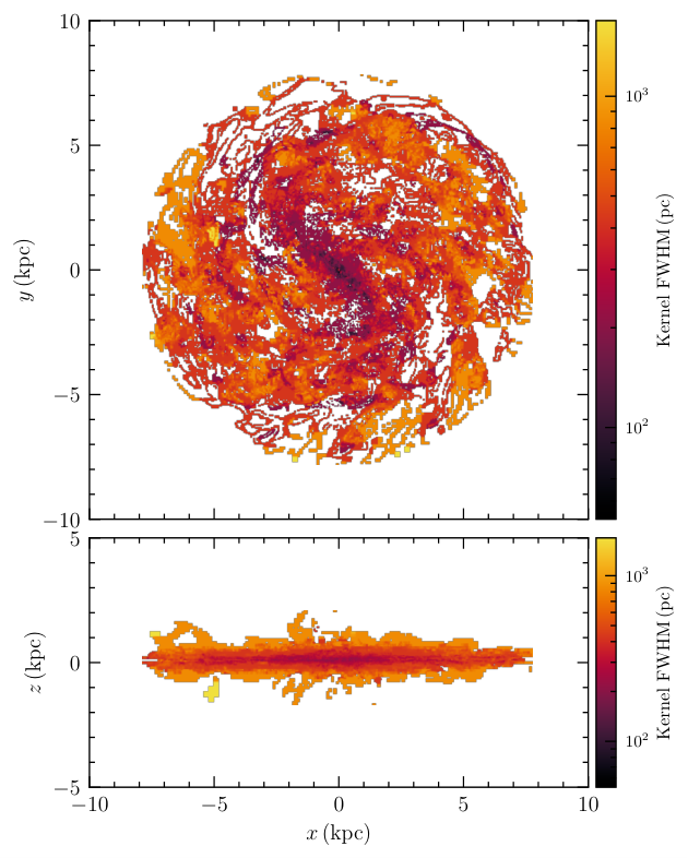
The choice of is a compromise. It must be large enough that each kernel contains sufficient cells for the dispersions in Eqs. (11)–(12) to be well sampled, and small enough to resolve the spatial variation of the turbulence quantities across the galaxy. To test the impact of this choice we repeated the full calculation for and , keeping and the ratio fixed so that the smoothing and weighting scales track the kernel.
Fig. 11 shows the resulting radial profiles of , and . As expected for turbulent fields, the first two are strongly scale dependent: both increase systematically with , since a larger kernel admits velocity and density fluctuations on larger scales. Their ratio, however, is far more stable. To quantify this we compare the five profiles of each quantity bin by bin: at a given radius we take the difference between the largest and smallest of the five values and divide it by their mean, and we then report the median of this fractional spread. The spread across – is 103% in and 86% in , but only 15% in . Crucially, the radial trend itself — solenoidal driving in the inner disc giving way to more compressive driving outwards — is present at every we tested, so none of the conclusions of Section 4 depend on this choice.
This behaviour is the same as that reported by Gerrard et al. (2023), and has a straightforward interpretation: and both change with the scale on which they are measured, in such a way that the change largely cancels in their ratio. The driving parameter is therefore a comparatively robust diagnostic, provided the kernel size is not varied by factors of several, in which case turbulence on a genuinely different scale is being probed.
We adopt as the smallest value for which the kernels are well populated: it yields a median of 292 cells per roving kernel, comfortably above the threshold of 30 imposed in Section 3, while keeping the kernel small enough to resolve structure on scales well below the disc scale length.