跳到论文正文
W Papers独立论文阅读器 arXiv:2609.14564 论文正文 计算阅读时间 · 0%
引用这篇论文根据当前论文元数据生成,正式投稿前建议核对。


License: CC BY 4.0
arXiv:2609.14564v1 [math.OC] 13 Sep 2026

A proximal linearized NEP method for composite optimization with conic and manifold constraints

Hao He Note: School of Mathematics, South China University of Technology, Guangzhou, China    Ruyu Liu and Shaohua Pan Note: School of Mathematics, South China University of Technology Note: School of Mathematics, South China University of Technology (shhpan@scut.edu.cn)
Abstract

This paper studies DC composite optimization problems with simultaneous conic and manifold constraints. We propose an inexact proximal linearized exact penalty algorithm based on a distance-based penalty function for the conic constraint. The algorithm successively computes approximate minimizers of proximal linearizations of the penalty function over the tangent spaces of the manifold under a readily verifiable inexactness criterion, with adaptive updates of the proximal and penalty parameters. Under the boundedness assumption on the sequences of iterates and penalty parameters, we establish an O⁡(ϵ−2)O(\epsilon^{-2}) worst-case complexity bound for finding an ϵ\epsilon-stationary point. Moreover, when semi-proximal ADMM is employed to solve the subproblems, the resulting oracle complexity is O⁡(ϵ−2​log⁡ϵ−1)O(\epsilon^{-2}\log\epsilon^{-1}) provided that the distance function and the first DC component are piecewise linear-quadratic, while an accelerated variant achieves an O⁡(ϵ−4)O(\epsilon^{-4}) oracle complexity. If, in addition, the associated potential function satisfies the KL property, the whole sequence of iterates converges to a stationary point. Extensive numerical experiments on composite optimization problems with orthogonal manifold, nonnegative cone, and second-order cone (SOC) constraints demonstrate the effectiveness of the proposed method.

Keywords: DC composite optimization; conic and/or manifold constraints; nonsmooth exact penalty; iteration and oracle complexity; global convergence

1 Introduction

Let 𝕏\mathbb{X} and 𝕐\mathbb{Y} denote real Euclidean spaces equipped with an inner product ⟨⋅,⋅⟩\langle\cdot,\cdot\rangle and its induced norm ∥⋅∥\|{}\cdot\|{}. Let ℳ⊂𝕏\mathcal{M}\subset\mathbb{X} be a closed 𝒞1\mathcal{C}^{1}-embedded submanifold, and let K⊂𝕐K\subset\mathbb{Y} be a simple closed convex set. We consider the following composite optimization problem:

minx∈ℳ∩g−1​(K)⁡Θ⁡(x):=f⁡(x)+ϑ⁡(x)−h⁡(x),\min_{x\in\mathcal{M}\cap g^{-1}(K)}\Theta(x):=f(x)+\vartheta(x)-h(x), (1)

where x∈g−1​(K)x\in g^{-1}(K) (or equivalently g⁡(x)∈Kg(x)\in K) represents the conic constraint, and the functions f,ϑ,h:𝕏→ℝf,\vartheta,h\!:\mathbb{X}\to\mathbb{R} and g:𝕏→𝕐g\!:\mathbb{X}\to\mathbb{Y} satisfy the conditions specified in Assumption 1.

Assumption 1

(i) ff is differentiable with locally Lipschitz gradient on an open convex set 𝒪⊃ℳ\mathcal{O}\supset\mathcal{M}, and gg is differentiable with locally Lipschitz Jacobian on 𝒪\mathcal{O};

(ii) ϑ\vartheta and hh are convex functions;

(iii) the feasible set ℳ∩g−1​(K)\mathcal{M}\cap g^{-1}(K) is assumed to be nonempty.

Model (1) provides a flexible framework for a broad class of problems, including cases where ϑ\vartheta is extended real-valued and cases in which ϑ\vartheta and hh are compositions of finite convex functions and smooth mappings. Due to the presence of the constraint x∈ℳx\in\mathcal{M}, model (1) does not fall within the DC composite optimization framework considered in [37, Eq. (46)]. Far from being merely abstract, this formulation arises naturally in a wide range of machine learning and scientific computing applications, as illustrated below.

Example 1

A representative application of manifold optimization arises in (row) sparse principal component analysis (see, e.g., [55, 32]), which can be formulated as

minX∈ℝn×p{−12tr(X⊤MX)+νφ(X)s.t.XX⊤v−v=0,X⊤X−I=0},\min_{X\in\mathbb{R}^{n\times p}}\Big\{-\frac{1}{2}{\rm tr}(X^{\top}MX)+\nu\varphi(X)\ \ {\rm s.t.}\ \ XX^{\top}v-v=0,\,X^{\top}X\!-\!I=0\Big\}, (2)

where MM is an n×nn\times n real symmetric data matrix, ν>0\nu>0 is a regularization parameter, φ\varphi is a convex (row) sparsity-promoting regularizer, v∈ℝnv\in\mathbb{R}^{n} is either a positive vector or the zero vector, and II denotes the identity matrix. Model (2) is a special case of (1) by setting h≡0,g⁡(X)=X​X⊤​v−v,𝕏=ℝn×p,ℳ=St⁡(n,p):={X∈ℝn×p|X⊤​X=I}h\equiv 0,g(X)=XX^{\top}v-v,\mathbb{X}=\mathbb{R}^{n\times p},\mathcal{M}={\rm St}(n,p):=\big\{X\in\mathbb{R}^{n\times p}\,|\,X^{\top}X=I\big\} and K={0}K=\{0\}. Alternatively, both constraints can be incorporated into the conic constraint by taking g⁡(X)=(X⊤​X−I,X​X⊤​v−v)g(X)=(X^{\top}X\!-\!I,XX^{\top}v-v), ℳ=𝕏=ℝn×p\mathcal{M}=\mathbb{X}=\mathbb{R}^{n\times p} and K={0}×{0}K=\{0\}\times\{0\}.

Example 2

The well-known kk-means clustering problem in unsupervised machine learning can equivalently be formulated as the following nonnegative orthogonal model [18]:

minX∈ℝn×p{f(X)s.t.X⊤X−I=0,X≥0,v∈span(X)},\min_{X\in\mathbb{R}^{n\times p}}\Big\{f(X)\ \ {\rm s.t.}\ \ X^{\top}X-I=0,\,X\geq 0,\,v\in{\rm span}(X)\Big\}, (3)

where f:ℝn×p→ℝf:\mathbb{R}^{n\times p}\to\mathbb{R} is a smooth function, X≥0X\geq 0 denotes the entrywise nonnegativity of matrix XX, and v∈ℝnv\in\mathbb{R}^{n} is a given positive vector. Model (3) therefore fits directly into the framework (1) by taking h≡0=ϑ,g⁡(X)=X,𝕏=𝕐=ℝn×p,ℳ=St⁡(n,p)h\equiv 0=\vartheta,g(X)=X,\mathbb{X}=\mathbb{Y}=\mathbb{R}^{n\times p},\mathcal{M}={\rm St}(n,p) and K=ℝ+n×pK=\mathbb{R}_{+}^{n\times p}, where ℝ+n×p\mathbb{R}_{+}^{n\times p} represents the nonnegative cone in ℝn×p\mathbb{R}^{n\times p}.

Example 3

A number of important optimization problems arising in machine learning and robust optimization can be formulated as second-order cone programs (SOCPs) involving DC regularizers and/or generalized sphere constraints (see, e.g., [43, 48]):

minx∈ℝn{f(x)+ϑ(x)−h(x)s.t.g(x)∈Km1×⋯×Kms,x⊤Bx=1}\min_{x\in\mathbb{R}^{n}}\Big\{f(x)+\vartheta(x)-h(x)\ \ {\rm s.t.}\ \ g(x)\in K^{m_{1}}\times\cdots\times K^{m_{s}},x^{\top}Bx=1\Big\} (4)

where f,ϑ,hf,\vartheta,h and gg are the same as in (1) with 𝕏=ℝn\mathbb{X}=\mathbb{R}^{n} and 𝕐=ℝm\mathbb{Y}=\mathbb{R}^{m} for m=m1+⋯+msm=m_{1}+\cdots+m_{s}, each Kmi:={(t,x)∈ℝ×ℝmi−1|‖x‖≤t}K^{m_{i}}:=\big\{(t,x)\in\mathbb{R}\times\mathbb{R}^{m_{i}-1}\ |\ \|x\|\leq t\big\} for i=1,…,si=1,\ldots,s is a second-order cone in ℝmi\mathbb{R}^{m_{i}}, and BB is an n×nn\times n real symmetric positive definite matrix. Clearly, model (4) is a special case of (1) with K=Km1×⋯×KmsK=K^{m_{1}}\times\cdots\times K^{m_{s}} and ℳ={x∈ℝn|x⊤​B​x=1}\mathcal{M}=\!\{x\in\mathbb{R}^{n}\,|\,x^{\top}Bx=1\}.

Example 4

Multiple nonnegative sparse canonical correlation analysis is formulated as

minX∈ℝ+n×p,Y∈ℝ+n×q−12​tr​(X⊤​A⊤​B​Y)+ν1​‖X‖2,1+ν2​‖Y‖2,1\displaystyle\min_{X\in\mathbb{R}_{+}^{n\times p},Y\in\mathbb{R}_{+}^{n\times q}}-\frac{1}{2}{\rm tr}(X^{\top}A^{\top}BY)+\nu_{1}\|X\|_{2,1}+\nu_{2}\|Y\|_{2,1}
s.t.X⊤​A⊤​A​X=1,Y⊤​B⊤​B​Y=1,\displaystyle\qquad\ \ {\rm s.t.}\ \ X^{\top}A^{\top}AX=1,Y^{\top}B^{\top}BY=1, (5)

where ∥X∥2,1:=∑i=1n∥Xi,:∥2\|X\|_{2,1}:=\sum_{i=1}^{n}\|X_{i,:}\|_{2} denotes the ℓ2,1\ell_{2,1}-norm of XX, and A∈ℝn×pA\in\mathbb{R}^{n\times p} and B∈ℝn×qB\in\mathbb{R}^{n\times q} are the data matrices, with A⊤​AA^{\top}A and B⊤​BB^{\top}B assumed to be positive definite. This problem can be viewed as a special case of (1) with 𝕏=ℝn×p×ℝn×p=𝕐,K=ℝ+n×p×ℝ+n×q\mathbb{X}=\mathbb{R}^{n\times p}\times\mathbb{R}^{n\times p}=\mathbb{Y},K=\mathbb{R}_{+}^{n\times p}\times\mathbb{R}_{+}^{n\times q} and ℳ={(X,Y)∈𝕏∣X⊤A⊤AX=1,Y⊤B⊤BY=1}\mathcal{M}=\!\{(X,Y)\in\mathbb{X}\mid X^{\top}A^{\top}AX=1,Y^{\top}B^{\top}BY=1\}. When the nonnegativity on matrices XX and YY are removed, it becomes the model considered in the reference [21].

Although problem (1) has been widely applied, solving it remains challenging due to the coexistence of the manifold constraint x∈ℳx\in\mathcal{M} and the conic constraint g⁡(x)∈Kg(x)\in K. We incorporate the conic constraint into the objective function through a nonsmooth penalty term, while preserving the manifold constraint in the feasible set and enforcing it algorithmically via retraction mappings. This leads to the following penalized problem

minx∈𝕏⁡Θρ​(x):=f⁡(x)+ϑ⁡(x)−h⁡(x)+ρ​dist​(g⁡(x),K)+δℳ​(x),\min_{x\in\mathbb{X}}\,\Theta_{\!\rho}(x):=f(x)+\vartheta(x)-h(x)+\rho\,{\rm dist}(g(x),K)+\delta_{\mathcal{M}}(x), (6)

where ρ>0\rho>0 is the penalty parameter, dist⁡(⋅,K){\rm dist}(\cdot,K) denotes the distance to KK induced by a norm |∥⋅∥||\!\lVert\cdot\lVert\!| on 𝕐\mathbb{Y} and the simplicity of KK ensures that dist⁡(⋅,K){\rm dist}(\cdot,K) admits an explicit expression, and δℳ​(⋅)\delta_{\mathcal{M}}(\cdot) denotes the indicator function of ℳ\mathcal{M}. As shown in Section 2.1, under a relatively weak constraint qualification (CQ), Θρ\Theta_{\rho} serves as a global exact penalty function; that is, there exists some ρ^>0\widehat{\rho}>0 such that, for every ρ≥ρ^\rho\geq\widehat{\rho}, the penalized problem shares the same set of global minimizers with (1). Unfortunately, the nonconvexity of Θρ\Theta_{\rho} for any fixed ρ\rho renders its global minimization computationally impractical. At the level of stationary points, Proposition 2.1 establishes a close correspondence between (1) and (6). This motivates us to seek a stationary point of (1) by solving a finite sequence of penalized problems.

1.1 Related research

The origins of nonsmooth penalty methods can be traced back to the early works of Eremin [26], Zangwill [58] and Pietrzykowski [49]. Subsequent studies by Charalambous [20], Han and Mangasarian [30], Coleman and Conn [22], and Bazaraa and Goode [6] established the exact penalty theory for classical nonlinear programming, which were later extended to general constrained optimization problems by Burke [16]. More recently, nonsmooth exact penalty methods have been investigated for a variety of challenging constrained optimization problems, including mathematical programs with equilibrium constraints (MPECs) [44, 45, 57], MPEC reformulations of zero-norm and rank regularized optimization problems [8, 42], and optimization problems with DC constraints [38, 28, 50].

A notable advantage of NEP methods for conic-constrained optimization problems (i.e., (1) with ϑ≡0≡h\vartheta\equiv 0\equiv h and ℳ=𝕏\mathcal{M}=\mathbb{X}) is that every KKT point of the original problem corresponds to a critical point of the penalized function for all sufficiently large penalty parameters; see Proposition 2.1. Motivated by this, Cartis et al. [19] proposed an NEP method based on the distance penalty function for conic-constrained optimization problems with K={0}K=\{0\} or ℝ+m\mathbb{R}_{+}^{m}. Their method successively computes an approximate solution of (6) with ρ=ρk\rho=\rho_{k} such that the stationarity measure is below a prescribed accuracy ϵ\epsilon, by employing either a trust-region or quadratic regularization approach, and subsequently updates the penalty parameter ρk\rho_{k} through a steering procedure [17]. They established worst-case iteration complexity bounds for finding either an ϵ\epsilon-approximate KKT point or an infeasible critical point of the feasibility measure dist⁡(g⁡(⋅),K){\rm dist}(g(\cdot),K). Specifically, an O⁡(ϵ−2)O(\epsilon^{-2}) bound was obtained when the penalty parameter sequence is bounded. When the penalty parameter sequence is unbounded but the iterate sequence is bounded, they derived an O⁡(ϵ−5)O(\epsilon^{-5}) bound.

For the same special case of (1), Diouane et al. [23] proposed an NEP method that successively computes an approximate solution of (6) with ρ=ρk\rho=\rho_{k} such that the stationarity measure is below a prescribed accuracy ϵk\epsilon_{k}, by applying a proximal modified quasi-Newton method [24]. Among others, each iteration of this second-order proximal method involves computing the proximal mapping of the composition ϑ∘𝒜j\vartheta\circ\mathcal{A}_{j}, where 𝒜j=g′​(xj)\mathcal{A}_{j}=g^{\prime}(x_{j}) is the Jacobian mapping of gg at the current iterate xjx_{j}, as well as an approximate minimizer of a quadratic function regularized by ϑ∘𝒜j\vartheta\circ\mathcal{A}_{j}. Subsequently, the accuracy requirement ϵk\epsilon_{k} and the penalty parameter ρk\rho_{k} are updated based on a feasibility measure that differs slightly from the one adopted in [19]. Assuming that the penalty parameter sequence satisfies a certain condition, which is automatically guaranteed under the MFCQ, they established an O⁡(|log⁡(ϵ/ϵ0)|​ϵ−2)O(|\log({\epsilon}/\epsilon_{0})|\epsilon^{-2}) worst-case iteration complexity bound for finding either an ϵ\epsilon-approximate KKT point or an infeasible critical point of the feasibility measure. In the unbounded case, the iteration complexity bound becomes O⁡(ϵ−8)O(\epsilon^{-8}), which is weaker than the complexity bound O⁡(ϵ−5)O(\epsilon^{-5}) obtained in [19] due to the use of a differently scaled feasibility measure.

It is worth noting that, for this special case of (1), worst-case iteration complexity bounds for obtaining approximate KKT points have also been established for an inexact proximal-point quadratic smooth penalty method under a global error bound in [40], as well as for smooth penalty methods with fixed penalty parameters under the LICQ in [14, 15]. However, these complexity results are generally weaker than the O⁡(ϵ−2)O(\epsilon^{-2}) iteration complexity bounds established for NEP methods in [19, 23]. Moreover, when ℳ=𝕏\mathcal{M}=\mathbb{X} and K=ℝ−K=\mathbb{R}_{-}, problem (1) reduces to a special case of the constrained difference programming problems studied in [46]. The extended SQP method (actually a nonsmooth penalty method) proposed therein employs exact solutions of subproblems and establishes the asymptotic convergence of the entire iterate sequence under the KL property. When ℳ=𝕏\mathcal{M}=\mathbb{X}, problem (1) also becomes a special case of the DC composite programs considered in [37], where a DC algorithm with adaptive penalty parameters is developed and subsequential convergence of the iterate sequence is established.

The aforementioned NEP methods are proposed for the special case of (1). They directly compute, at each outer iteration, an approximate solution of the penalized problem with the stationarity measure below a prescribed accuracy. However, directly solving each penalized problem remains challenging due to its nonsmooth and composite structure. Motivated by this challenge, we develop an efficient algorithm for (1) by successively minimizing proximal linearizations of the penalized functions {Θρk}k≥0\{\Theta_{\rho_{k}}\}_{k\geq 0}, with adaptive updates of the proximal and penalty parameters throughout the iterations. Specifically, at the kk-th iteration, we construct a proximal linearization Θ^ρk​(⋅,xk)\widehat{\Theta}_{\rho_{k}}(\cdot;x^{k}) of Θρk\Theta_{\rho_{k}} at xk∈ℳx^{k}\!\in\mathcal{M} by replacing ff and gg with their first-order approximations at xkx^{k}, replacing −h-h by its majorant associated with some ζk∈∂(−h)​(xk)\zeta^{k}\in\partial(-h)(x^{k}), and adding a proximal term βk2∥⋅−xk∥2\frac{\beta_{k}}{2}\|\cdot-x^{k}\|^{2}. An approximate minimizer vk∈Txk​ℳv^{k}\in T_{x^{k}}\mathcal{M} of Θ^ρk​(xk+v,xk)\widehat{\Theta}_{\rho_{k}}(x^{k}\!+v;x^{k}) is then computed according to a practical inexactness criterion, and a candidate point is generated by applying the retraction Rxk​(⋅)R_{x^{k}}(\cdot) to vkv^{k}. The resulting candidate point is accepted as the next iterate only if it yields sufficient decrease in Θρk\Theta_{\rho_{k}}. Otherwise, the proximal parameter βk\beta_{k} is adaptively increased to construct a new proximal linearization of Θρk\Theta_{\rho_{k}} at xkx^{k} until the required decrease is attained. Subsequently, the penalty parameter ρk\rho_{k} is adaptively updated based on the current constraint violation, resulting in a new penalized problem with ρk+1\rho_{k+1}, and the above procedure is repeated.

1.2 Main contributions

The main contributions of this work are as follows.

(i) We develop a proximal linearized nonsmooth exact penalty framework for DC composite optimization problems with conic and manifold constraints. Unlike the existing NEP methods in [19, 23], which directly solve a sequence of penalized problems to prescribed stationarity accuracy, the proposed iPLNEP method only requires approximate solutions of strongly convex proximal linearized subproblems on the tangent spaces of the manifold. The inexactness of these subproblems is characterized by a readily implementable KKT-residual-based criterion, which can be naturally achieved by standard convex optimization solvers. This design yields an implementable double-loop framework while retaining the favorable complexity properties of NEP methods.

(ii) We establish the worst-case iteration complexity of iPLNEP. Under the boundedness assumption on the iterate and penalty parameter sequences, iPLNEP requires at most O⁡(ϵ−2)O(\epsilon^{-2}) iterations to find an ϵ\epsilon-stationary point of (1). This matches the complexity order established for existing NEP methods [19, 23] in special cases of the considered model, although the proposed method does not compute approximate stationary points of the penalized problems themselves. The analysis is nontrivial since the stationarity properties of the proximal linearized subproblems do not directly translate into those of the penalized problems.

(iii) We derive the overall oracle complexity of iPLNEP when the proximal linearized subproblems are solved by the semi-proximal ADMM and its accelerated variant. When the semi-proximal ADMM in [27, Appendix B] is employed, we establish an overall oracle complexity of O⁡(ϵ−2​log⁡ϵ−1)O(\epsilon^{-2}\log\epsilon^{-1}) provided that both ϑ⁡(⋅)\vartheta(\cdot) and dist⁡(⋅,K){\rm dist}(\cdot,K) are piecewise linear quadratic functions. When the accelerated semi-proximal ADMM in [53] is employed, an O⁡(ϵ−4)O(\epsilon^{-4}) overall oracle complexity is obtained without requiring these additional structural assumptions. These oracle complexity bounds rely on standard first-order oracles for evaluating g′​(xk)​(⋅)g^{\prime}(x^{k})(\cdot), ∇g​(xk)​(⋅)\nabla g(x^{k})(\cdot), 𝒫σk−1​ϑ​(⋅)\mathcal{P}_{\sigma_{k}^{-1}\vartheta}(\cdot), 𝒫σk−1​ρk​dist​(⋅,K)​(⋅)\mathcal{P}_{\sigma_{k}^{-1}\rho_{k}{\rm dist}(\cdot,K)}(\cdot), and 𝒫Txk​ℳ​(⋅)\mathcal{P}_{T_{x^{k}}\mathcal{M}}(\cdot) at each iteration, thereby demonstrating the computational tractability of the proposed framework.

(iv) The convergence of the entire iterate sequence is established under the KL property of the constructed potential function. This result complements existing convergence analyses of NEP-type methods by allowing inexact subproblem solutions and adaptive updates of the proximal and penalty parameters. In particular, compared with the subsequential convergence result in [37, Theorem 4], our analysis further provides KL-based convergence of the whole sequence and nonasymptotic complexity guarantees. We further note that, when ℳ=𝕏\mathcal{M}=\mathbb{X} and K=ℝ−K=\mathbb{R}_{-}, the proposed algorithm shares a similar proximal linearization framework with the inexact proximal linearized DC algorithm in [56, Section 2.2]. However, the inexactness criterion employed in our method differs from that used therein. Moreover, the main emphasis of this work is on establishing iteration complexity guarantees, whereas [56] mainly investigates asymptotic convergence properties.

We apply iPLNEP equipped with the (accelerated) semi-proximal ADMM as the subproblem solver to solve Examples 1-3 on synthetic and real datasets. Its performance is evaluated against PenCPG [55] and LSALM [59] for row-sparse PCA, I-AManPG [32] for community detection, RALM [2] for kk-means clustering, a SeDuMi-based DC algorithm [43] for DC regularized SOCPs, and IPOPT [54] for synthetic nonconvex SOCPs involving a generalized sphere constraint. Numerical results demonstrate that iPLNEP achieves lower constraint violations and comparable solution quality for row-sparse PCA, slightly better clustering performance with competitive efficiency for kk-means clustering, and superior scalability for nonconvex SOCPs.

1.3 Notation

Throughout this paper, ℝn×p\mathbb{R}^{n\times p} denotes the space of n×pn\times p real matrices equipped with the standard trace inner product and the induced Frobenius norm ∥⋅∥F\|\cdot\|_{F}, while ℤ:=𝕏×𝕐\mathbb{Z}:=\mathbb{X}\times\mathbb{Y} is equipped with the norm ‖z‖:=‖x‖2+‖y‖2\|z\|:=\!\sqrt{\|x\|^{2}\!+\!\|y\|^{2}} for z=(x,y)z=(x;y). We use ℐ\mathcal{I} to denote the identity mapping. For a positive semidefinite (PSD) linear operator 𝒬\mathcal{Q}, ∥⋅∥𝒬\|\cdot\|_{\mathcal{Q}} denotes the seminorm defined by ∥⋅∥𝒬:=⟨⋅,𝒬⋅⟩\|\cdot\|_{\mathcal{Q}}:=\sqrt{\langle\cdot,\mathcal{Q}\cdot\rangle}. Let ℕ\mathbb{N} and ℕ+\mathbb{N}_{+} denote the sets of nonnegative integers and positive integers, respectively. For any k∈ℕ+k\in\mathbb{N}_{+}, we write [k]:={0,…,k}[k]:=\{0,\ldots,k\} and [k]+:={1,…,k}[k]_{+}:=\{1,\ldots,k\}. For any x,x′∈𝕏x,x^{\prime}\in\mathbb{X}, [x,x′][x,x^{\prime}] denotes the line segment joining xx and x′x^{\prime}. For a closed set C⊂𝕏C\subset\mathbb{X}, let δC\delta_{C} denote its indicator function, defined by δC​(x)=0\delta_{C}(x)=0 if x∈Cx\in C and δC​(x)=∞\delta_{C}(x)=\infty otherwise, and let 𝒫C\mathcal{P}_{C} denote the projection mapping onto CC. For x∈𝕏x\in\mathbb{X} and δ>0\delta>0, let 𝔹⁡(x,δ)\mathbb{B}(x,\delta) and 𝔹¯​(x,δ)\overline{\mathbb{B}}(x,\delta) denote the open and closed balls centered at xx with radius δ\delta, respectively. We also write 𝔹¯𝕏:=𝔹¯​(0,1)\overline{\mathbb{B}}_{\mathbb{X}}:=\overline{\mathbb{B}}(0,1). For a mapping g:𝕏→𝕐g\!:\mathbb{X}\to\mathbb{Y} and a point x∈𝕏x\in\mathbb{X}, if gg is differentiable at xx, ∇g​(x)\nabla g(x) denotes the adjoint of the differential g′​(x):𝕏→𝕐g^{\prime}(x)\!:\mathbb{X}\to\mathbb{Y} of gg at xx. For any x∈ℳx\in\mathcal{M}, Tx​ℳT_{x}\mathcal{M} and Nx​ℳN_{x}\mathcal{M} denote the tangent and normal spaces to ℳ\mathcal{M} at xx, respectively. For a proper function ϕ:𝕏→ℝ¯:=(−∞,∞]\phi\!:\mathbb{X}\to\overline{\mathbb{R}}:=(-\infty,\infty] and a point x∈dom​ϕx\in{\rm dom}\,\phi, where dom​ϕ:={x∈𝕏|ϕ⁡(x)<∞}{\rm dom}\,\phi:=\big\{x\in\mathbb{X}\ |\ \phi(x)<\infty\big\}, ∂ϕ⁡(x)\partial\phi(x) denotes the (limiting) subdifferential of ϕ\phi at xx. When ϕ\phi is the indicator function of a closed set C⊂𝕏C\subset\mathbb{X}, ∂ϕ⁡(x)\partial\phi(x) coincides with the normal cone to CC at xx, denoted by 𝒩C​(x)\mathcal{N}_{C}(x). In particular, when C=ℳC=\mathcal{M}, we write 𝒩ℳ​(x)\mathcal{N}_{\mathcal{M}}(x) as Nx​ℳN_{x}\mathcal{M}. For a closed and proper function φ:𝕏→ℝ¯\varphi:\mathbb{X}\to\overline{\mathbb{R}}, its proximal mapping with parameter γ>0\gamma>0 is defined as 𝒫γ​φ(⋅):=arg⁡minx′∈𝕏{φ(x′)+12​γ∥x′−⋅∥2}\mathcal{P}_{\gamma\varphi}(\cdot)\!:=\mathop{\arg\min}_{x^{\prime}\in\mathbb{X}}\big\{\varphi(x^{\prime})+\frac{1}{2\gamma}\|x^{\prime}-\cdot\|^{2}\big\}.

2 Preliminaries

We introduce an extended CQ for (1) and establish the global exactness of (6) under a suitable subregularity CQ. We then define stationary points for (1) and (6), and discuss the relationship between them. Finally, several properties of retractions are recalled.

2.1 CQs and global exact penalty

Definition 2.1

For problem (1), we say that the extended CQ holds at a point x¯∈ℳ\overline{x}\in\mathcal{M} if both ξ¯∈𝒩K​(𝒫K​(g⁡(x¯)))\overline{\xi}\in\mathcal{N}_{K}(\mathcal{P}_{K}(g(\overline{x}))) and 0∈∇g​(x¯)​ξ¯+Nx¯​ℳ0\in\nabla g(\overline{x})\overline{\xi}+N_{\overline{x}}\mathcal{M} imply ξ¯=0\overline{\xi}=0, where 𝒫K​(⋅)\mathcal{P}_{K}(\cdot) denotes the projection mapping onto KK induced by |∥⋅∥||\!\lVert\cdot\lVert\!|. If 𝒫K\mathcal{P}_{K} is not single-valued, it is understood that 𝒫K​(g​(x¯))\mathcal{P}_{K}(g(\overline{x})) denotes an arbitrary projection of g⁡(x¯)g(\overline{x}) onto KK.

When ℳ=𝕏\mathcal{M}=\mathbb{X}, the extended CQ in Definition 2.1 reduces to the CQ in [37, Eq. (53)], and further to the standard MFCQ when 𝕏=ℝn\mathbb{X}=\mathbb{R}^{n} and g⁡(x¯)∈K=ℝ+mg(\overline{x})\in K=\mathbb{R}_{+}^{m}. If x¯∈ℳ∩g−1​(K)\overline{x}\in\mathcal{M}\cap g^{-1}(K), it coincides with the CQ in [51, Example 9.44], specialized to F⁡(x):=(g⁡(x),x)F(x)\!:=(g(x);x) for x∈𝕏x\in\mathbb{X} and D=K×ℳD\!=K\times\mathcal{M}. The latter is equivalent to the metric regularity of the multifunction ℱ⁡(⋅):=F⁡(⋅)−D\mathcal{F}(\cdot):=F(\cdot)-D at (x¯,0)∈gph​ℱ(\overline{x},0)\in{\rm gph}\,\mathcal{F}, and is stronger than the metric subregularity of ℱ\mathcal{F} at this point. Recall that a multifunction ℋ:𝕏⇉𝕐\mathcal{H}\!:\mathbb{X}\rightrightarrows\mathbb{Y} is said to be metrically subregular at a point (x¯,y¯)∈gph​ℋ(\overline{x},\overline{y})\in{\rm gph}\,\mathcal{H} with constant κ≥0\kappa\geq 0 if there exists ε>0\varepsilon>0 such that

dist⁡(x,ℋ−1​(y¯))≤κ​dist​(y¯,ℋ⁡(x))for​all​x∈𝔹¯​(x¯,ε).{\rm dist}(x,\mathcal{H}^{-1}(\overline{y}))\leq\kappa{\rm dist}(\overline{y},\mathcal{H}(x))\quad{\rm for\ all}\ x\in\overline{\mathbb{B}}(\overline{x},\varepsilon).

For x¯∈ℳ∩g−1​(K)\overline{x}\in\!\mathcal{M}\cap g^{-1}(K), it follows directly from this definition that the metric subregularity of ℱ\mathcal{F} at (x¯,0)(\overline{x},0) implies that of the multifunction 𝒢\mathcal{G} at (x¯,0)(\overline{x},0), where 𝒢\mathcal{G} is defined by

𝒢⁡(x):={g⁡(x)−Kif​x∈ℳ,∅otherwise.\mathcal{G}(x):=\left\{\begin{array}[]{cl}g(x)-K&{\rm if}\ x\in\mathcal{M},\\ \emptyset&{\rm otherwise}.\end{array}\right. (7)

Consequently, the extended CQ of (1) at x¯∈ℳ∩g−1​(K)\overline{x}\in\mathcal{M}\cap g^{-1}(K) implies the subregularity of 𝒢\mathcal{G} at (x¯,0)(\overline{x},0), which is precisely the subregularity CQ for (1) at x¯\overline{x}.

We next show that (6) is a global exact penalty of (1) under the subregularity CQ.

Lemma 2.1

Let S∗S^{*} denote the set of global optimal solutions of (1). Suppose that the mapping 𝒢\mathcal{G} defined in (7) is metrically subregular at any (x,0)(x,0) with x∈S∗x\in S^{*}, and that Θ\Theta is coercive or the manifold ℳ\mathcal{M} is compact. Then, (6) is a global exact penalty of (1).

Proof: By [25, Theorem 3H.3], the metric subregularity of a multifunction ℋ:𝕏⇉𝕐\mathcal{H}\!:\mathbb{X}\rightrightarrows\mathbb{Y} at (x¯,y¯)∈gph​ℋ(\overline{x},\overline{y})\in{\rm gph}\,\mathcal{H} is equivalent to the calmness of its inverse ℋ−1:𝕐⇉𝕏\mathcal{H}^{-1}:\mathbb{Y}\rightrightarrows\mathbb{X} at (y¯,x¯)(\overline{y},\overline{x}) with the same constant κ\kappa, i.e., there exists δ>0\delta>0 such that for all y∈𝕐y\in\mathbb{Y},

ℋ−1​(y)∩𝔹⁡(x¯,δ)⊂ℋ−1​(y¯)+κ​‖y−y¯‖​𝔹¯𝕏.\mathcal{H}^{-1}(y)\cap\mathbb{B}(\overline{x},\delta)\subset\mathcal{H}^{-1}(\overline{y})+\kappa\|y-\overline{y}\|\overline{\mathbb{B}}_{\mathbb{X}}.

Let ℋ⁡(τ):={x∈ℳ|dist⁡(g⁡(x),K)=τ}\mathcal{H}(\tau):=\big\{x\in\mathcal{M}\ |\ {\rm dist}(g(x),K)=\tau\big\} for τ≥0\tau\geq 0. Fix any x¯∈ℳ∩g−1​(K)=ℋ⁡(0)\overline{x}\in\mathcal{M}\cap g^{-1}(K)=\mathcal{H}(0). By the definitions of calmness and metric subregularity, it is straightforward to verify that such ℋ\mathcal{H} is calm at (0,x¯)(0,\overline{x}) if and only if 𝒢−1\mathcal{G}^{-1} is calm at (0,x¯)(0,\overline{x}). Hence, for any given x∈S∗x\in S^{*}, the metric subregularity of 𝒢\mathcal{G} at (x,0)(x,0) is equivalent to the calmness of ℋ\mathcal{H} at (0,x)(0,x). Invoking [42, Lemma 2.1 & Proposition 2.1 (b)], (6) is a global exact penalty of (1). □\Box

2.2 Stationary points

Let Θ~:=Θ+δK∘g+δℳ\widetilde{\Theta}:=\Theta+\delta_{K}\circ g+\delta_{\mathcal{M}} denote the extended-real-valued objective function of (1). By [51, Theorem 10.1], any local optimal solution x∗x^{*} satisfies 0∈∂Θ~​(x∗)0\in\partial\widetilde{\Theta}(x^{*}). Under Assumption 1, the function Θ\Theta is locally Lipschitz continuous, and at every x∈ℳ∩g−1​(K)x\in\mathcal{M}\cap g^{-1}(K), ∂Θ~​(x)⊂∂Θ⁡(x)+∂(δK∘g+δℳ)​(x)\partial\widetilde{\Theta}(x)\subset\partial\Theta(x)+\partial(\delta_{K}\circ g+\delta_{\mathcal{M}})(x) and ∂Θ⁡(x)⊂∇f​(x)+∂ϑ⁡(x)+∂(−h)​(x)\partial\Theta(x)\subset\nabla\!f(x)+\partial\vartheta(x)+\partial(-h)(x), where the inclusions follow from [51, Exercise 10.10]. Further, if the mapping 𝒢\mathcal{G} in (7) is metrically subregular at (x,0)(x,0) for x∈ℳ∩g−1​(K)x\in\mathcal{M}\cap g^{-1}(K), then by [33, Section 3.1] the inclusion ∂(δK∘g+δℳ)​(x)⊂∇g​(x)​𝒩K​(g⁡(x))+Nx​ℳ\partial(\delta_{K}\circ g+\delta_{\mathcal{M}})(x)\subset\nabla g(x)\mathcal{N}_{K}(g(x))+N_{x}\mathcal{M} holds. Therefore, if 𝒢\mathcal{G} is metrically subregular at (x∗,0)(x^{*},0),

0∈∂Θ~​(x∗)⊂∇f​(x∗)+∂ϑ⁡(x∗)+∂(−h)​(x∗)+∇g​(x∗)​𝒩K​(g⁡(x∗))+Nx∗​ℳ.0\in\partial\widetilde{\Theta}(x^{*})\subset\nabla\!f(x^{*})+\partial\vartheta(x^{*})+\partial(-h)(x^{*})+\nabla g(x^{*})\mathcal{N}_{K}(g(x^{*}))+N_{x^{*}}\mathcal{M}.

This inclusion naturally motivates the following notions of stationary points for (1).

Definition 2.2

(i) A point xx is called a stationary point of (1) if x∈ℳ∩g−1​(K)x\in\mathcal{M}\cap g^{-1}(K) and there exists ξ∈𝒩K​(g​(x))\xi\in\mathcal{N}_{K}(g(x)) such that 0∈∇f​(x)+∂ϑ⁡(x)+∂(−h)​(x)+∇g​(x)​ξ+Nx​ℳ0\in\nabla\!f(x)+\partial\vartheta(x)+\partial(-h)(x)+\nabla g(x)\xi+N_{x}\mathcal{M} or, equivalently, 0∈𝒫Tx​ℳ​[∇f​(x)+∂ϑ⁡(x)+∂(−h)​(x)+∇g​(x)​ξ]0\in\mathcal{P}_{T_{x}\mathcal{M}}\big[\nabla\!f(x)+\partial\vartheta(x)+\partial(-h)(x)+\nabla g(x)\xi\big].

(ii) For ϵ≥0\epsilon\geq 0, a point xx is called an ϵ\epsilon-stationary point of (1) if x∈ℳx\in\mathcal{M} and there exist z∈𝕏,y∈K,ζ∈∂(−h)​(x),ξ1∈∂ϑ⁡(z)z\in\mathbb{X},y\in K,\zeta\in\partial(-h)(x),\xi_{1}\in\partial\vartheta(z) and ξ2∈𝒩K​(y)\xi_{2}\in\mathcal{N}_{K}(y) such that

‖x−z‖≤ϵ,‖g⁡(x)−y‖≤ϵ​and​‖𝒫Tx​ℳ​[∇f​(x)+ζ+ξ1+∇g​(x)​ξ2]‖≤ϵ.\|x-z\|\leq\epsilon,\,\|g(x)-y\|\leq\epsilon\ {\rm and}\ \|\mathcal{P}_{T_{x}\mathcal{M}}\left[\nabla\!f(x)+\zeta+\xi_{1}+\nabla g(x)\xi_{2}\right]\|\leq\epsilon.

For given ρ>0\rho>0 and x∈ℳx\in\mathcal{M}, it follows from [51, Exercise 10.10] that ∂(Θρ+δℳ)​(x)⊂∂Θρ​(x)+Nx​ℳ⊂∇f​(x)+∂ϑ⁡(x)+∂(−h)​(x)+ρ​∂(dist⁡(g⁡(⋅),K))​(x)+Nx​ℳ\partial(\Theta_{\rho}\!+\!\delta_{\mathcal{M}})(x)\!\subset\partial\Theta_{\rho}(x)+N_{x}\mathcal{M}\subset\nabla\!f(x)+\partial\vartheta(x)+\partial(-h)(x)+\rho\partial({\rm dist}(g(\cdot),K))(x)+N_{x}\mathcal{M}, and the inclusion is generally strict due to the nonconvex −h-h. This motivates the following notions of stationary points for the penalty problem (6).

Definition 2.3

For a given ρ>0\rho>0, a point xx is called a stationary point of problem (6) if x∈ℳx\in\mathcal{M} and 0∈∂Θρ​(x)+Nx​ℳ0\in\partial\Theta_{\rho}(x)+N_{x}\mathcal{M}, and a weak stationary point of (6) if x∈ℳx\in\mathcal{M} and 0∈∇f​(x)+∂ϑ⁡(x)+ρ​∂(dist⁡(g⁡(⋅),K))​(x)+∂(−h)​(x)+Nx​ℳ0\in\nabla\!f(x)+\partial\vartheta(x)+\rho\partial({\rm dist}(g(\cdot),K))(x)+\partial(-h)(x)+N_{x}\mathcal{M}.

To establish the relationship between the stationary points of (1) and those of (6), we first recall the subdifferential of dist⁡(⋅,K){\rm dist}(\cdot,K) in the following lemma. The lemma follows directly by applying [51, Theorem 10.13] to the function (y,z)↦|∥y−z∥|+δK​(y)(y,z)\mapsto|\!\lVert y-z\rVert\!|+\delta_{K}(y).

Lemma 2.2

At any y¯∈𝕐\overline{y}\in\mathbb{Y}, ∂dist(y¯,K)=⋃x∗∈𝒫K​(y¯)[(−∂|∥⋅∥|(x∗−y¯))∩𝒩K(x∗)]\partial{\rm dist}(\overline{y},K)=\bigcup_{x^{*}\in\mathcal{P}_{K}(\overline{y})}[(-\partial|\!\lVert\cdot\lVert\!|(x^{*}\!-\!\overline{y}))\cap\mathcal{N}_{K}(x^{*})] if y¯∉K\overline{y}\notin K; otherwise, ∂dist(y¯,K)={u∈𝒩K(y¯)∣|∥u∥|∗≤1}\partial{\rm dist}(\overline{y},K)=\{u\in\mathcal{N}_{K}(\overline{y})\mid|\!\lVert u\lVert\!|_{*}\leq 1\}, where |∥⋅∥|∗|\!\lVert\cdot\lVert\!|_{*} is the dual norm of |∥⋅∥||\!\lVert\cdot\lVert\!|.

Proposition 2.1

A stationary point x¯\overline{x} of (1) is a weak stationary point of (6) for all sufficiently large ρ\rho. Conversely, a weak stationary point x¯\overline{x} of (6) satisfying g⁡(x¯)∈Kg(\overline{x})\in K is a stationary point of (1). If the objective function of (1) does not involve −h-h, the same relations hold between the stationary points of (1) and (6).

Proof: The Lipschitz continuity of dist⁡(⋅,K){\rm dist}(\cdot,K), together with [51, Theorem 10.6], implies

∂(dist⁡(g⁡(⋅),K))​(x)=∇g​(x)​∂dist⁡(g⁡(x),K)for​all​x∈𝕏.\partial({\rm dist}(g(\cdot),K))(x)=\nabla g(x)\partial{\rm dist}(g(x),K)\quad{\rm for\ all}\ x\in\mathbb{X}. (8)

Suppose that x¯\overline{x} is a stationary point of (1). By Definition 2.2 (i), x¯∈ℳ∩g−1​(K)\overline{x}\in\mathcal{M}\cap g^{-1}(K) and there exists some ξ∈𝒩K​(g​(x¯))\xi\in\mathcal{N}_{K}(g(\overline{x})) such that 0∈∇f​(x¯)+∂ϑ⁡(x¯)+∇g​(x¯)​ξ+∂(−h)​(x¯)+Nx¯​ℳ0\in\nabla\!f(\overline{x})+\partial\vartheta(\overline{x})+\nabla g(\overline{x})\xi+\partial(-h)(\overline{x})+N_{\overline{x}}\mathcal{M}. Choose ρξ≥|∥ξ∥|∗\rho_{\xi}\geq|\!\lVert\xi\lVert\!|_{*}. Since ξ∈𝒩K​(g​(x¯))\xi\in\mathcal{N}_{K}(g(\overline{x})), Lemma 2.2 yields ρ−1​ξ∈∂dist⁡(g⁡(x¯),K)\rho^{-1}\xi\in\partial{\rm dist}(g(\overline{x}),K) for all ρ≥ρξ\rho\geq\rho_{\xi}. It then follows from (8) that ∇g​(x¯)​ξ∈ρ​∂(dist⁡(g⁡(⋅),K))​(x¯)\nabla g(\overline{x})\xi\in\rho\partial({\rm dist}(g(\cdot),K))(\overline{x}) for all ρ≥ρξ\rho\geq\rho_{\xi}. Consequently, 0∈∇f​(x¯)+∂ϑ⁡(x¯)+ρ​∂(dist⁡(g⁡(⋅),K))​(x¯)+∂(−h)​(x¯)+Nx¯​ℳ0\in\nabla\!f(\overline{x})+\partial\vartheta(\overline{x})+\rho\partial({\rm dist}(g(\cdot),K))(\overline{x})+\partial(-h)(\overline{x})+N_{\overline{x}}\mathcal{M}. This shows that x¯\overline{x} is a weak stationary point of (6) for all ρ≥ρξ\rho\geq\rho_{\xi}. Conversely, suppose that x¯∈ℳ\overline{x}\in\mathcal{M} is a weak stationary point of (6) for ρ>0\rho>0 satisfying g⁡(x¯)∈Kg(\overline{x})\in K. By Definition 2.3, Lemma 2.2, and (8), we obtain 0∈∇f​(x¯)+∂ϑ⁡(x¯)+∇g​(x¯)​𝒩K​(g⁡(x¯))+∂(−h)​(x¯)+Nx¯​ℳ0\in\nabla\!f(\overline{x})+\partial\vartheta(\overline{x})+\nabla g(\overline{x})\mathcal{N}_{K}(g(\overline{x}))+\partial(-h)(\overline{x})+N_{\overline{x}}\mathcal{M}. Definition 2.2 then implies that x¯\overline{x} is a stationary point of (1). The last part follows by noting that ∂Θρ​(x)=∇f​(x)+∂ϑ⁡(x)+ρ​∂(dist⁡(g⁡(⋅),K))​(x)\partial\Theta_{\rho}(x)=\nabla\!f(x)+\partial\vartheta(x)+\rho\partial({\rm dist}(g(\cdot),K))(x) for all x∈𝕏x\in\mathbb{X}. □\Box

To close this section, we recall the definition of a retraction, which serves as a first-order approximation to the exponential mapping on a Riemannian manifold. Retractions will be employed in our algorithm to ensure that all iterates remain on the manifold ℳ\mathcal{M}.

Definition 2.4

(see [1, Definition 4.1]) Let R:T​ℳ→ℳR:T\mathcal{M}\to\mathcal{M} be a smooth mapping, where T​ℳT\mathcal{M} denotes the tangent bundle of ℳ\mathcal{M}. The mapping RR is called a retraction if its restriction Rx​(⋅):=R⁡(x,⋅):Tx​ℳ→ℳR_{x}(\cdot):=R(x,\cdot):T_{x}\mathcal{M}\to\mathcal{M} satisfies Rx​(0)=xR_{x}(0)=x and Rx′​(0)=ℐR_{x}^{\prime}(0)=\mathcal{I}.

Recall that ℳ\mathcal{M} is a closed 𝒞1\mathcal{C}^{1}-embedded submanifold of 𝕏\mathbb{X}. The local representation of ℳ\mathcal{M} implies that the projection mapping 𝒫Tx​ℳ\mathcal{P}_{T_{x}\mathcal{M}} is continuous in x∈ℳx\in\mathcal{M}. The following basic properties of retractions will also be used in the subsequent analysis. Since their proofs are similar to those in [12, Appendix B], we omit the details.

Lemma 2.3

For any compact set Λ⊂ℳ,δ>0\varLambda\subset\mathcal{M},\delta>0, and retraction RR on ℳ\mathcal{M}, there exist constants M1,M2>0M_{1},M_{2}>0 such that, for every x∈Λx\in\varLambda and v∈Tx​ℳ∩𝔹¯​(0,δ)v\in T_{x}\mathcal{M}\cap\overline{\mathbb{B}}(0,\delta),

‖Rx​(v)−x‖≤M1​‖v‖and‖Rx​(v)−x−v‖≤M2​‖v‖2.\|R_{x}(v)-x\|\leq M_{1}\|v\|\ \ {\rm and}\ \ \|R_{x}(v)-x-v\|\leq M_{2}\|v\|^{2}.

3 An inexact proximal linearized NEP method

Let xk∈ℳx^{k}\in\!\mathcal{M} be the current iterate, and let ρk\rho_{k} denote the associated penalty parameter. We first construct a proximal linearization of the penalty function Θρk\Theta_{\!\rho_{k}} at xkx^{k}. Under Assumption 1 (i), we define the first-order local models of ff and gg around xkx^{k} as follows:

ℓf(⋅;xk):=f(xk)+⟨∇f(xk),⋅−xk⟩andℓg(⋅;xk):=g(xk)+g′(xk)(⋅−xk).\ell_{f}(\cdot;x^{k}):=f(x^{k})+\langle\nabla\!f(x^{k}),\cdot-x^{k}\rangle\ \ {\rm and}\ \ \ell_{g}(\cdot;x^{k}):=g(x^{k})+g^{\prime}(x^{k})(\cdot-x^{k}).

Choose an arbitrary ζk∈∂(−h)​(xk)\zeta^{k}\in\partial(-h)(x^{k}). Since −ζk∈∂h⁡(xk)-\zeta^{k}\in\partial h(x^{k}) and hh is convex, we have

−h⁡(x)≤−h⁡(xk)+⟨ζk,x−xk⟩∀x∈𝕏.-h(x)\leq-h(x^{k})+\langle\zeta^{k},x-x^{k}\rangle\quad\forall x\in\mathbb{X}.

Consequently, we define the following proximal linearization of Θρk\Theta_{\!\rho_{k}} at xkx^{k}:

Θ^ρk​(x,xk):=ℓf​(x,xk)+ϑ⁡(x)+ρk​dist​(ℓg​(x,xk),K)−h⁡(xk)+⟨ζk,x−xk⟩+βk2​‖x−xk‖2,\displaystyle\widehat{\Theta}_{\!\rho_{k}}(x;x^{k})\!:=\ell_{f}(x;x^{k})+\vartheta(x)+\rho_{k}\mathrm{dist}(\ell_{g}(x;x^{k}),K)-h(x^{k})+\langle\zeta^{k},x\!-\!x^{k}\rangle+\frac{\beta_{k}}{2}\|x-x^{k}\|^{2},

where βk>0\beta_{k}>0 is a proximal parameter. The proximal term βk2∥⋅−xk∥2\frac{\beta_{k}}{2}\|\cdot-x^{k}\|^{2} is incorporated to ensure the strong convexity of Θ^ρk​(⋅,xk)\widehat{\Theta}_{\!\rho_{k}}(\cdot;x^{k}), which facilitates the computation of an approximate solution to the resulting subproblem. It is worth noting that Θ^ρk​(⋅,xk)\widehat{\Theta}_{\!\rho_{k}}(\cdot;x^{k}) does not necessarily majorize Θρk\Theta_{\rho_{k}} around xkx^{k} unless βk\beta_{k} is sufficiently large, depending on the Lipschitz moduli of ∇f\nabla\!f and g′g^{\prime} at xkx^{k}, as well as the penalty parameter ρk\rho_{k}.

The proposed linearized NEP method computes a search direction vk∈Txk​ℳv^{k}\in T_{x^{k}}\mathcal{M} by approximately solving the following strongly convex subproblem

minv∈Txk​ℳ⁡Θ^ρk​(xk+v,xk)=ℓk​(v)+ϑ⁡(xk+v)+ρk​dist​(ℓg​(xk+v,xk),K)+βk2​‖v‖2,\min_{v\in T_{\!x^{k}}\mathcal{M}}\widehat{\Theta}_{\!\rho_{k}}(x^{k}\!+v;x^{k})=\ell_{k}(v)+\vartheta(x^{k}\!+v)+\rho_{k}{\rm dist}(\ell_{g}(x^{k}\!+v;x^{k}),K)+\frac{\beta_{k}}{2}\|v\|^{2}, (9)

where ℓk​(v):=⟨∇f​(xk)+ζk,v⟩+f⁡(xk)−h⁡(xk)\ell_{k}(v):=\langle\nabla\!f(x^{k})\!+\!\zeta^{k},v\rangle+f(x^{k})-h(x^{k}) for v∈𝕏v\in\mathbb{X}. To measure the optimality of an approximate solution of (9), we reformulate the subproblem as

minv∈𝕏,z∈ℤ⁡ℓk​(v)+ψρk​(z)+δTxk​ℳ​(v)+βk2​‖v‖2\displaystyle\min_{v\in\mathbb{X},z\in\mathbb{Z}}\,\ell_{k}(v)+\psi_{\rho_{k}}(z)+\delta_{T_{\!x^{k}}\mathcal{M}}(v)+\frac{\beta_{k}}{2}\|v\|^{2}
s.t.G⁡(xk,v)−z=0withG⁡(x,v):=(x+vℓg​(x+v,x)),\displaystyle\quad{\rm s.t.}\ \ G(x^{k},v)-z=0\quad\ {\rm with}\ \ G(x,v):=\begin{pmatrix}x+v\\ \ell_{g}(x\!+\!v;x)\end{pmatrix}, (10)

where ψρk​(z):=ϑ⁡(z1)+ρk​dist​(z2,K)\psi_{\rho_{k}}(z):=\vartheta(z_{1})+\rho_{k}{\rm dist}(z_{2},K) for z=(z1,z2)∈ℤz=(z_{1},z_{2})\in\mathbb{Z}. Since (10) is a convex optimization problem in (v,z)(v,z), a pair (vk,∗,zk,∗)∈Txk​ℳ×ℤ(v^{k,*},z^{k,*})\in T_{\!x^{k}}\mathcal{M}\times\mathbb{Z} is an optimal solution if and only if there exists ξk,∗∈∂ψρk​(zk,∗)\xi^{k,*}\in\partial\psi_{\rho_{k}}(z^{k,*}) such that

G⁡(xk,vk,∗)−zk,∗=0and𝒫Txk​ℳ​(∇ℓk​(vk,∗)+βk​vk,∗+∇vG​(xk,vk,∗)​ξk,∗)=0.G(x^{k},v^{k,*})-z^{k,*}=0\ \ {\rm and}\ \ \mathcal{P}_{T_{\!x^{k}}\mathcal{M}}\big(\nabla\ell_{k}(v^{k,*})+\beta_{k}v^{k,*}\!+\!\nabla_{\!v}G(x^{k},v^{k,*})\xi^{k,*}\big)=0.

Let v¯k\overline{v}^{k} denote the unique optimal solution of subproblem (9). We next formulate an inexactness criterion for computing vkv^{k} based on whether v¯k=0\overline{v}^{k}=0. If v¯k=0\overline{v}^{k}=0, the optimality condition of (9) implies that xkx^{k} is a critical point of the penalty function Θρk\Theta_{\rho_{k}}. Now it is reasonable to require the approximate solution vk∈Txk​ℳv^{k}\in T_{x^{k}}\mathcal{M} to be small in norm. Accordingly, we call vk∈Txk​ℳv^{k}\in T_{x^{k}}\mathcal{M} an acceptable approximate solution of (9) if there exist zk∈ℤz^{k}\in\mathbb{Z} and ξk∈∂ψρk​(zk)\xi^{k}\in\partial\psi_{\rho_{k}}(z^{k}) such that, for a prescribed tolerance εk>0\varepsilon_{k}>0,

max⁡{‖G⁡(xk,vk)−zk‖,‖𝒫Txk​ℳ​(∇ℓk​(vk)+βk​vk+∇vG​(xk,vk)​ξk)‖,‖βk​vk‖}≤εk.\max\big\{\|G(x^{k},v^{k})\!-\!z^{k}\|,\|\mathcal{P}_{T_{\!x^{k}}\mathcal{M}}(\nabla\ell_{k}(v^{k})+\beta_{k}v^{k}+\!\nabla_{\!v}G(x^{k},v^{k})\xi^{k})\|,\|\beta_{k}v^{k}\|\big\}\leq\varepsilon_{k}. (11)

The term ‖βk​vk‖\|{}\beta_{k}v^{k}\| is included to control the step size ‖vk‖\|{}v^{k}\|{}. When v¯k≠0\overline{v}^{k}\neq 0, it is natural to require vkv^{k} to provide a sufficient descent for Θ^ρk​(⋅,xk)\widehat{\Theta}_{\rho_{k}}(\cdot;x^{k}) at xkx^{k}, namely,

Θ^ρk​(xk+vk,xk)<Θ^ρk​(xk,xk)=Θρk​(xk).\widehat{\Theta}_{\rho_{k}}(x^{k}\!+v^{k};x^{k})<\widehat{\Theta}_{\rho_{k}}(x^{k};x^{k})=\Theta_{\rho_{k}}(x^{k}). (12)

Meanwhile, a natural way to quantify the inexactness of vk∈Txk​ℳv^{k}\in T_{x^{k}}\mathcal{M} as an approximate solution of (9) is to require the existence of zk∈ℤz^{k}\in\mathbb{Z} and ξk∈∂ψρk​(zk)\xi^{k}\in\partial\psi_{\rho_{k}}(z^{k}) such that

‖G⁡(xk,vk)−zk‖≤ak​‖vk‖2​and​‖𝒫Txk​ℳ​(∇ℓk​(vk)+βk​vk+∇vG​(xk,vk)​ξk)‖≤bk​‖vk‖,\|G(x^{k},v^{k})-z^{k}\|\!\leq a_{k}\|v^{k}\|^{2}\ {\rm and}\ \big\|\mathcal{P}_{T_{\!x^{k}}\mathcal{M}}(\nabla\ell_{k}(v^{k})+\beta_{k}v^{k}\!+\nabla_{\!v}G(x^{k},v^{k})\xi^{k})\big\|\leq\!b_{k}\|v^{k}\|, (13)

where ak>0a_{k}>0 and bk>0b_{k}>0 are prescribed constants. Here, the constraint residual ‖G⁡(xk,vk)−zk‖\|G(x^{k},v^{k})-z^{k}\| is required to be of order O⁡(‖vk‖2)O(\|v^{k}\|^{2}) rather than merely O⁡(‖vk‖)O(\|v^{k}\|). A second-order control of the constraint residual is imposed, which is essential for establishing Lemma 3.3 and the subsequent iteration complexity bounds. In summary, at the kk-th iteration, the proposed method inexactly solves the strongly convex subproblem (9), or equivalently (10), to obtain a triple (vk,zk,ξk)∈Txk​ℳ×ℤ×∂ψρk​(zk)(v^{k},z^{k},\xi^{k})\in T_{x^{k}}\mathcal{M}\times\mathbb{Z}\times\partial\psi_{\rho_{k}}(z^{k}) that satisfies either the inexactness criterion (11) or the alternative conditions (12)-(13). Subsequently, a candidate point is constructed as Rxk​(vk)R_{x^{k}}(v^{k}) through the retraction Rxk​(⋅)R_{x^{k}}(\cdot).

Note that βk\beta_{k} controls the curvature of the proximal linearization Θ^ρk​(⋅,xk)\widehat{\Theta}_{\!\rho_{k}}(\cdot;x^{k}), and consequently affecting its local approximation accuracy and the quality of the candidate point Rxk​(vk)R_{x^{k}}(v^{k}). Following a strategy similar to that in [19, Algorithm 2.2], we adaptively update βk\beta_{k}. Specifically, define the actual and predicted decreases as

aredk:=Θρk​(xk)−Θρk​(Rxk​(vk))andpredk:=Θρk​(xk)−Θ^ρk​(xk+vk,xk).{\rm ared}_{k}:=\Theta_{\rho_{k}}(x^{k})-\Theta_{\rho_{k}}(R_{x^{k}}(v^{k}))\ \ {\rm and}\ \ {\rm pred}_{k}\!:=\Theta_{\rho_{k}}(x^{k})-\widehat{\Theta}_{\rho_{k}}(x^{k}\!+\!v^{k};x^{k}). (14)

If predk<γ¯∥vk∥2\text{pred}_{k}<\overline{\gamma}\|{}v^{k}\|{}^{2} for some γ¯>0\overline{\gamma}>0, or if the ratio aredk/predk\text{ared}_{k}/\text{pred}_{k} falls below a prescribed threshold, then βk\beta_{k} is regarded as insufficiently large to yield an accurate local approximation of Θρk​(⋅)\Theta_{\!\rho_{k}}(\cdot). In this case, the candidate point Rxk​(vk)R_{x^{k}}(v^{k}) is rejected and βk\beta_{k} is increased. Otherwise, the candidate point Rxk​(vk)R_{x^{k}}(v^{k}) is accepted, and βk\beta_{k} is either kept unchanged or reduced slightly. The penalty parameter ρk\rho_{k} is updated according to the feasibility violation measured by dist⁡(z2k,K){\rm dist}(z_{2}^{k},K). Specifically, under the inexactness criterion (11), we increase ρk\rho_{k} whenever dist​(z2k,K)>εk\text{dist}(z_{2}^{k},K)>\varepsilon_{k}. Under the criterion given by (12)-(13), since ‖g⁡(xk)+g′​(xk)​vk−z2k‖≤ak​‖vk‖2\|{}g(x^{k})+g^{\prime}(x^{k})v^{k}-z_{2}^{k}\|{}\leq a_{k}\|v^{k}\|^{2}, we increase ρk\rho_{k} whenever dist​(z2k,K)>βk​‖vk‖\text{dist}(z_{2}^{k},K)>\beta_{k}\|{}v^{k}\|{}. These considerations motivate the following algorithm.

1: Input: a retraction RR, parameters ρ0>0,0​<βmin​<β0,amax>​0,bmax>​0,τ>1\rho_{0}>0,0<\beta_{\rm min}<\beta_{0},a_{\max}\!>0,b_{\max}\!>0,\tau>1,      ε0>0,ς∈(0,1),0<η1<η2​<1,γ¯>​0,0<σ2<1<σ1\varepsilon_{0}>0,\varsigma\in(0,1),0<\!\eta_{1}<\eta_{2}<1,\overline{\gamma}>0,0<\!\sigma_{2}<1<\sigma_{1}, and x0∈ℳx^{0}\in\mathcal{M}.
2: for k=0,1,2,…k=0,1,2,\ldots do
3:   Choose ζk∈∂(−h)​(xk)\zeta^{k}\in\partial(-h)(x^{k}).
4:   Select ak∈(0,amax]a_{k}\in(0,a_{\max}] and bk∈(0,bmax]b_{k}\in(0,b_{\max}]. Solve the subproblem (10) inexactly to     obtain (vk,zk,ξk)∈Txk​ℳ×ℤ×∂ψρk​(zk)(v^{k},z^{k},\xi^{k})\in T_{x^{k}}\mathcal{M}\times\mathbb{Z}\times\partial\psi_{\rho_{k}}(z^{k}) such that either (11) or both (12) and     (13) hold. For the former, go to Step 5; otherwise, go to Step 6.
5:   If max⁡{εk,dist⁡(z2k,K)}=0\max\{\varepsilon_{k},{\rm dist}(z_{2}^{k},K)\}=0, then stop. Otherwise, if dist⁡(z2k,K)≤εk{\rm dist}(z_{2}^{k},K)\leq\varepsilon_{k}, then     set xk+1:=xk,βk+1:=βk,ρk+1:=ρk,εk+1:=ς​εkx^{k+1}\!:=x^{k},\beta_{k+1}\!:=\beta_{k},\rho_{k+1}\!:=\rho_{k},\varepsilon_{k+1}\!:=\varsigma\varepsilon_{k}, and go to Step 2; else set    xk+1:=xk,βk+1:=βk,ρk+1:=τ​ρk,εk+1:=ς​εkx^{k+1}\!:=x^{k},\beta_{k+1}\!:=\beta_{k},\rho_{k+1}\!:=\tau\rho_{k},\varepsilon_{k+1}\!:=\varsigma\varepsilon_{k}, and go to Step 2.
6:   If max⁡{‖vk‖,dist⁡(z2k,K)}=0\max\{\|v^{k}\|,{\rm dist}(z_{2}^{k},K)\}=0, then stop.
7:   Compute rk:=aredk/predkr_{k}:={{\rm ared}_{k}}/{{\rm pred}_{k}}. If rk<η1r_{k}<\eta_{1} or predk<γ¯​‖vk‖2{\rm pred}_{k}<\overline{\gamma}\|v^{k}\|^{2}, set xk+1:=xkx^{k+1}:=x^{k},     βk+1:=σ1​βk,ρk+1:=ρk\beta_{k+1}:=\sigma_{1}\beta_{k},\rho_{k+1}:=\rho_{k}, and go to Step 2. Otherwise, set xk+1:=Rxk​(vk)x^{k+1}:=R_{x^{k}}(v^{k}) and
βk+1:={βkif​rk<η2,#​s​u​c​c​e​s​s​f​u​lmax⁡{σ2​βk,βmin} otherwise.#​v​e​r​y​s​u​c​c​e​s​s​f​u​l\beta_{k+1}:=\left\{\begin{array}[]{cl}\beta_{k}&\text{if}\ r_{k}<\eta_{2},\qquad{\#successful}\\ \max\{\sigma_{2}\beta_{k},\beta_{\min}\}&\text{ otherwise}.\qquad{\#very\ successful}\end{array}\right. (15)
8:   Update the penalty parameter ρk+1\rho_{k+1} via the following rule
ρk+1:={τ​ρkif​max⁡{ρk,[dist⁡(z2k,K)]−1}<βk−1​‖vk‖−1,ρkotherwise.\rho_{k+1}:=\left\{\begin{aligned} \tau\rho_{k}\quad&{\rm if}\,\,\max\{\rho_{k},[{\rm dist}(z_{2}^{k},K)]^{-1}\}<\beta_{k}^{-1}\|v^{k}\|^{-1},\\ \rho_{k}\quad\,\,&{\rm otherwise}.\end{aligned}\right. (16)
9: end for
Algorithm 1 (Inexact nonsmooth penalty method)
Remark 3.1

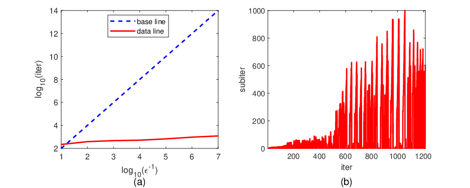
(a) As shown in Appendix A, for each k∈ℕk\in\mathbb{N}, applying a convergent solver (e.g., an accelerated proximal gradient method) to the dual of subproblem (10) produces, after finitely many iterations, a triplet (vk,zk,ξk)∈Txk​ℳ×ℤ×∂ψρk​(zk)(v^{k},z^{k},\xi^{k})\in T_{x^{k}}\mathcal{M}\times\mathbb{Z}\times\partial\psi_{\rho_{k}}(z^{k}) satisfying either the inexactness criterion (11) or the alternative criterion given by (12)-(13). A similar finite-iteration guarantee is established for the (accelerated) semi-proximal ADMM discussed in Section 6.1.1. These results demonstrate that the proposed inexactness criteria are practically implementable, as they can be attained in finitely many iterations by standard subproblem solvers. The combination of (12) and (13) is inspired by [41]. To accommodate the additional conic constraint g⁡(x)∈Kg(x)\in K, we also allow vkv^{k} to satisfy the inexactness criterion (11), which is essential for establishing the oracle complexity bound of Algorithm 1 to compute a feasible ϵ\epsilon-stationary point. As illustrated in Figure 1 (a), this additional criterion is invoked only at a small number of iterations.

Refer to caption
Figure 1: (a) Inexactness conditions across iterations: “inc 1” denotes satisfaction of (11), and “inc 2” denotes satisfaction of both (12) and (13). (b) Successful and unsuccessful iterations throughout the algorithm: “uns 1” denotes a failure in Step 5; “uns 2” denotes a failure in Step 7 due to predk<γ¯​‖vk‖\operatorname{pred}_{k}<\overline{\gamma}\|v^{k}\|; “uns 3” denotes a failure in Step 7 due to rk<η1r_{k}<\eta_{1}; and “s” denotes a successful or very successful step. This figure is depicted by running Algorithm 1 for (56).

(b) When Step 7 is executed, the triplet (vk,zk,ξk)∈Txk​ℳ×ℤ×∂ψρk​(zk)(v^{k},z^{k},\xi^{k})\in T_{x^{k}}\mathcal{M}\times\mathbb{Z}\times\partial\psi_{\rho_{k}}(z^{k}) necessarily satisfies the inexactness criterion formed by (12)-(13). Consequently, predk>0{\rm pred}_{k}>0, and hence the ratio rk=aredk/predkr_{k}={\rm ared}_{k}/{\rm pred}_{k} is well-defined. If rk<η1r_{k}<\eta_{1} or predk<γ¯∥vk∥2{\rm pred}_{k}<\overline{\gamma}\|{}v^{k}\|{}^{2}, indicating an unsatisfactory model decrease or an insufficient predicted decrease, respectively, then βk+1\beta_{k+1} is increased so that Θ^ρk+1​(⋅,xk+1)\widehat{\Theta}_{\rho_{k+1}}(\cdot;x^{k+1}) provides a sufficiently accurate local approximation to Θρk+1​(⋅)\Theta_{\rho_{k+1}}(\cdot) at the unchanged iterate xk+1=xkx^{k+1}=x^{k}. Otherwise, it follows from the definition of rkr_{k} that the sufficient-decrease condition

Θρk​(xk)−Θρk​(Rxk​(vk))≥γ¯​η1​‖vk‖2,\Theta_{\rho_{k}}(x^{k})-\Theta_{\rho_{k}}(R_{x^{k}}(v^{k}))\geq\overline{\gamma}\eta_{1}\|v^{k}\|^{2}, (17)

holds, and βk+1\beta_{k+1} is subsequently updated according to rkr_{k} as specified in (15). Finally, the iterative scheme of Algorithm 1 ensures that βk≥βmin\beta_{k}\geq\beta_{\rm min} for all k∈ℕk\in\mathbb{N}.

(c) Let 𝒮:={k∈ℕ∣xk+1=Rxk​(vk)}\mathcal{S}:=\{k\in\mathbb{N}\mid x^{k+1}=R_{x^{k}}(v^{k})\} denote the set of successful iteration indices. By the iterative mechanism of Algorithm 1, for each k∈𝒮k\in\mathcal{S}, the triplet (vk,zk,ξk)∈Txk​ℳ×ℤ×∂ψρk​(zk)(v^{k},z^{k},\xi^{k})\in T_{x^{k}}\mathcal{M}\times\mathbb{Z}\times\partial\psi_{\rho_{k}}(z^{k}) satisfies (12)-(13), and the sufficient-decrease condition (17) holds. Moreover, for every k∉𝒮k\notin\mathcal{S}, we have xk+1=xk=xk′x^{k+1}=x^{k}=x^{k^{\prime}} for some k′∈𝒮k^{\prime}\in\mathcal{S} with k′<kk^{\prime}<k. Hence, the unsuccessful iterations merely repeat an iterate generated at a successful iteration, and the set of accumulation points of {xk}k∈ℕ\{x^{k}\}_{k\in\mathbb{N}} coincides with that of {xk}k∈𝒮\{x^{k}\}_{k\in\mathcal{S}}. Figure 1 (b) illustrates the successful and unsuccessful iterations throughout the algorithm. We observe that most of the unsuccessful iterations are triggered by the condition rk<η1r_{k}<\eta_{1} in Step 7.

(d) If max⁡{εk,dist⁡(z2k,K)}=0\max\{\varepsilon_{k},{\rm dist}(z_{2}^{k},K)\}=0, then xkx^{k} is necessarily a stationary point of (1). Indeed, whenever Step 5 is executed, the triplet (vk,zk,ξk)∈Txk​ℳ×ℤ×∂ψρk​(zk)(v^{k},z^{k},\xi^{k})\in T_{x^{k}}\mathcal{M}\times\mathbb{Z}\times\partial\psi_{\rho_{k}}(z^{k}) satisfies (11), which, together with εk=0\varepsilon_{k}=0 and dist⁡(z2k,K)=0{\rm dist}(z_{2}^{k},K)=0, yields the stationarity conditions in Definition 2.2. Likewise, if max⁡{‖vk‖,dist⁡(z2k,K)}=0\max\{\|v^{k}\|,{\rm dist}(z_{2}^{k},K)\}=0, then xkx^{k} is also a stationary point of (1). In this case, the iterative mechanism of Algorithm 1 ensures that (vk,zk,ξk)∈Txk​ℳ×ℤ×∂ψρk​(zk)(v^{k},z^{k},\xi^{k})\in T_{x^{k}}\mathcal{M}\times\mathbb{Z}\times\partial\psi_{\rho_{k}}(z^{k}) satisfies (13). Since vk=0v^{k}=0, (13) implies that z1k=xk,g⁡(xk)=z2k∈Kz^{k}_{1}=x^{k},g(x^{k})=z_{2}^{k}\in K and 0∈∇f​(xk)+∂ϑ⁡(xk)+∂(−h)​(xk)+∇g​(xk)​𝒩K​(g⁡(xk))+Nxk​ℳ0\in\nabla\!f(x^{k})+\partial\vartheta(x^{k})+\partial(-h)(x^{k})+\nabla\!g(x^{k})\mathcal{N}_{K}(g(x^{k}))+N_{x^{k}}\mathcal{M}. Thus, xkx^{k} is a stationary point of (1) by Definition 2.2. This explains the use of max⁡{εk,dist⁡(z2k,K)}=0\max\{\varepsilon_{k},{\rm dist}(z_{2}^{k},K)\}=0 or max⁡{‖vk‖,dist⁡(z2k,K)}=0\max\{\|v^{k}\|,{\rm dist}(z_{2}^{k},K)\}=0 is used as the stopping condition in Algorithm 1.

Remark 3.2

When ℳ=𝕏\mathcal{M}=\mathbb{X}, there is no need to split the nonsmooth functions ϑ(xk+⋅)\vartheta(x^{k}\!+\cdot) and δTxk​ℳ​(⋅)\delta_{T_{x^{k}}\mathcal{M}}(\cdot) in (10), so the mapping G⁡(x,⋅)G(x,\cdot) defined there simplifies to ℓg​(x+v,x)\ell_{g}(x+v;x). In this case, the inexactness conditions (11) and (13) are respectively replaced by

max⁡{‖(xk+vk−sk,ℓg​(xk+vk,xk)−zk)‖,‖xk+vk−sk‖,‖βk​vk‖}≤εk,\displaystyle\max\big\{\|(x^{k}\!+\!v^{k}-s^{k};\ell_{g}(x^{k}\!+\!v^{k};x^{k})-z^{k})\|,\|x^{k}\!+\!v^{k}-s^{k}\|,\|\beta_{k}v^{k}\|\big\}\leq\varepsilon_{k},
‖(xk+vk−sk,ℓg​(xk+vk,xk)−zk)‖≤ak​‖vk‖2​and​‖xk+vk−sk‖≤bk​‖vk‖,\displaystyle\|(x^{k}\!+\!v^{k}-s^{k};\ell_{g}(x^{k}\!+\!v^{k};x^{k})-z^{k})\|\leq\!a_{k}\|v^{k}\|^{2}\ {\rm and}\ \big\|x^{k}\!+\!v^{k}-s^{k}\big\|\!\leq b_{k}\|v^{k}\|,

where sk:=𝒫ϑ​(xk+vk−∇ℓk​(vk)−βk​vk−∇g​(xk)​ξk)s^{k}:=\mathcal{P}_{\vartheta}\big(x^{k}+v^{k}-\!\nabla\ell_{k}(v^{k})\!-\!\beta_{k}v^{k}-\nabla g(x^{k})\xi^{k}\big) with ξk∈ρk​∂dist⁡(zk,K)\xi^{k}\in\rho_{k}\partial{\rm dist}(z^{k},K).

Since dist⁡(⋅,K){\rm dist}(\cdot,K) is 11-Lipschitz continuous w.r.t. |∥⋅∥||\!\lVert\cdot\rVert\!| and all norms on the finite-dimensional space 𝕐\mathbb{Y} are equivalent, there exist constants cu≥cl>0c_{u}\geq c_{l}>0 such that

cl∥⋅∥≤|∥⋅∥|≤cu∥⋅∥,|dist(y1,K)−dist(y2,K)|≤cu∥y1−y2∥∀y1,y2∈𝕐.c_{l}\|\cdot\|\leq|\!\lVert\cdot\rVert\!|\leq c_{u}\|\cdot\|,\ |{\rm dist}(y^{1},K)-{\rm dist}(y^{2},K)|\leq c_{u}\|y^{1}-y^{2}\|\quad\forall y^{1},y^{2}\in\mathbb{Y}. (18)

Combining the second inequality in (18) with the definition of ψρk\psi_{\rho_{k}}, we obtain the following estimate, which will be frequently invoked in the subsequent analysis.

Lemma 3.1

Consider a compact convex set Ω⊂𝕏\Omega\subset\mathbb{X} and let γ\gamma be a Lipschitz constant of ϑ\vartheta on Ω\Omega. Then, for each k∈ℕk\in\mathbb{N}, ψρk\psi_{\rho_{k}} is Lipschitz continuous on Ω×𝕐\Omega\times\mathbb{Y} with

|ψρk​(z1)−ψρk​(z2)|≤(γ2+cu2​ρk2)1/2​‖z1−z2‖∀z1,z2∈Ω×𝕐.|\psi_{\rho_{k}}(z^{1})-\psi_{\rho_{k}}(z^{2})|\leq\big(\gamma^{2}\!+\!c_{u}^{2}\rho_{k}^{2}\big)^{1/2}\|z^{1}-z^{2}\|\quad\forall z^{1},z^{2}\in\Omega\times\mathbb{Y}.

We next present two lemmas that will be used to establish Lemma 4.2. Specifically, Lemma 3.2 offers a lower bound for Θ^ρk​(xk+v,xk)−Θ^ρk​(xk+vk,xk)\widehat{\Theta}_{\rho_{k}}(x^{k}\!+\!v;x^{k})-\widehat{\Theta}_{\rho_{k}}(x^{k}\!+\!v^{k};x^{k}) for v∈Txk​ℳv\in T_{x^{k}}\mathcal{M}, while Lemma 3.3 provides an upper bound for Θρk​(Rxk​(vk))−Θ^ρk​(xk+vk,xk)\Theta_{\rho_{k}}(R_{x^{k}}(v^{k}))-\widehat{\Theta}_{\rho_{k}}(x^{k}\!+\!v^{k};x^{k}).

Lemma 3.2

Fix any k∈ℕk\in\mathbb{N} for which (vk,zk,ξk)∈Txk​ℳ×ℤ×∂ψρk​(zk)(v^{k},z^{k},\xi^{k})\!\in T_{x^{k}}\mathcal{M}\times\mathbb{Z}\times\partial\psi_{\rho_{k}}(z^{k}) satisfies (12)-(13). Let L~ϑ,k\widetilde{L}_{\vartheta,k} denote the Lipschitz modulus of ϑ\vartheta on the line segment [xk+vk,z1k][x^{k}\!+\!v^{k},z_{1}^{k}]. Then

Θ^ρk​(xk+v,xk)−Θ^ρk​(xk+vk,xk)\displaystyle\widehat{\Theta}_{\rho_{k}}(x^{k}\!+\!v;x^{k})-\widehat{\Theta}_{\rho_{k}}(x^{k}\!+\!v^{k};x^{k}) ≥(βk/2)​‖v−vk‖2−bk​‖vk‖​‖v−vk‖\displaystyle\geq({\beta_{k}}/{2})\|v\!-\!v^{k}\|^{2}-b_{k}\|v^{k}\|\|v\!-\!v^{k}\|
−2​ak​(L~ϑ,k2+cu2​ρk2)1/2​‖vk‖2∀v∈Txk​ℳ.\displaystyle\quad\ -2a_{k}(\widetilde{L}_{\vartheta,k}^{2}\!+\!c_{u}^{2}\rho_{k}^{2})^{1/2}\|v^{k}\|^{2}\quad\ \forall v\in T_{x^{k}}\mathcal{M}.

Proof: Fix any ϵ>0\epsilon>0. Since ϑ\vartheta is Lipschitz continuous on [xk+vk,z1k][x^{k}\!+\!v^{k},z_{1}^{k}] with Lipschitz constant L~ϑ,k+ϵ\widetilde{L}_{\vartheta,k}\!+\epsilon, it follows from Lemma 3.1, ξk∈∂ψρk​(zk)\xi^{k}\in\partial\psi_{\rho_{k}}(z^{k}) and [51, Theorem 9.13] that ‖ξk‖≤[(L~ϑ,k+ϵ)2+cu2​ρk2]1/2\|\xi^{k}\|\leq[(\widetilde{L}_{\vartheta,k}\!+\!\epsilon)^{2}\!+\!c_{u}^{2}\rho_{k}^{2}]^{1/2}. Together with the first inequality in (13), it follows

|ψρk​(zk)−ψρk​(G⁡(xk,vk))+⟨ξk,G⁡(xk,vk)−zk⟩|≤2​ak​[(L~ϑ,k+ϵ)2+cu2​ρk2]1/2​‖vk‖2.\big|\psi_{\rho_{k}}(z^{k})-\psi_{\rho_{k}}(G(x^{k},v^{k}))+\langle\xi^{k},G(x^{k},v^{k})-z^{k}\rangle\big|\leq 2a_{k}[(\widetilde{L}_{\vartheta,k}\!+\!\epsilon)^{2}\!+\!c_{u}^{2}\rho_{k}^{2}]^{1/2}\|v^{k}\|^{2}. (19)

Fix any v∈Txk​ℳv\in T_{x^{k}}\mathcal{M}. Since ℓk(⋅)+βk2∥⋅∥2+δTxk​ℳ(⋅)\ell_{k}(\cdot)+\frac{\beta_{k}}{2}\|\cdot\|^{2}+\delta_{T_{\!x^{k}}\mathcal{M}}(\cdot) is βk\beta_{k}-strongly convexity, we have

ℓk​(v)+βk2​‖v‖2≥ℓk​(vk)+βk2​‖vk‖2+⟨∇ℓk​(vk)+βk​vk+s,v−vk⟩+βk2​‖v−vk‖2\ell_{k}(v)+\frac{\beta_{k}}{2}\|v\|^{2}\geq\ell_{k}(v^{k})+\frac{\beta_{k}}{2}\|v^{k}\|^{2}+\langle\nabla\ell_{k}(v^{k})+\beta_{k}v^{k}+s,v-v^{k}\rangle+\frac{\beta_{k}}{2}\|v-v^{k}\|^{2}

for any s∈𝒩Txk​ℳ​(vk)s\in\mathcal{N}_{T_{x^{k}}\mathcal{M}}(v^{k}). Moreover, ξk∈∂ψρk​(zk)\xi^{k}\in\partial\psi_{\rho_{k}}(z^{k}) and the convexity of ψρk​(⋅)\psi_{\rho_{k}}(\cdot) yield

ψρk​(G⁡(xk,v))\displaystyle\psi_{\rho_{k}}(G(x^{k},v)) ≥ψρk​(zk)+⟨ξk,G⁡(xk,vk)−zk⟩+⟨ξk,G⁡(xk,v)−G⁡(xk,vk)⟩\displaystyle\geq\psi_{\rho_{k}}(z^{k})+\langle\xi^{k},G(x^{k},v^{k})-z^{k}\rangle+\langle\xi^{k},G(x^{k},v)-G(x^{k},v^{k})\rangle
=ψρk​(zk)+⟨ξk,G⁡(xk,vk)−zk⟩+⟨∇vG​(xk,vk)​ξk,v−vk⟩,\displaystyle=\psi_{\rho_{k}}(z^{k})+\langle\xi^{k},G(x^{k},v^{k})-z^{k}\rangle+\langle\nabla_{\!v}G(x^{k},v^{k})\xi^{k},v-v^{k}\rangle,

where the equality is due to the affinity of G⁡(xk,⋅)G(x^{k},\cdot). Adding the above two inequalities together and using the relation Θ^ρk(xk+⋅;xk)=ℓk(⋅)+βk2∥⋅∥2+ψρk(G(xk,⋅))\widehat{\Theta}_{\!\rho_{k}}(x^{k}\!+\!\cdot;x^{k})=\ell_{k}(\cdot)+\frac{\beta_{k}}{2}\|\cdot\|^{2}+\psi_{\rho_{k}}(G(x^{k},\cdot)) gives

Θ^ρk​(xk+v,xk)\displaystyle\widehat{\!\Theta}_{\rho_{k}}(x^{k}\!+\!v;x^{k}) ≥Θ^ρk​(xk+vk,xk)+ψρk​(zk)−ψρk​(G⁡(xk,vk))+⟨ξk,G⁡(xk,vk)−zk⟩\displaystyle\geq\widehat{\Theta}_{\rho_{k}}(x^{k}\!+\!v^{k};x^{k})+\psi_{\rho_{k}}(z^{k})-\psi_{\rho_{k}}(G(x^{k},v^{k}))+\langle\xi^{k},G(x^{k},v^{k})-z^{k}\rangle
+βk2​‖v−vk‖2+⟨∇ℓk​(vk)+βk​vk+∇vG​(xk,vk)​ξk+s,v−vk⟩\displaystyle\quad+\frac{\beta_{k}}{2}\|v-v^{k}\|^{2}+\langle\nabla\ell_{k}(v^{k})+\beta_{k}v^{k}+\nabla_{\!v}G(x^{k},v^{k})\xi^{k}\!+s,v-v^{k}\rangle
≥Θ^ρk​(xk+vk,xk)+⟨∇ℓk​(vk)+βk​vk+∇vG​(xk,vk)​ξk+s,v−vk⟩\displaystyle\geq\widehat{\Theta}_{\rho_{k}}(x^{k}\!+\!v^{k};x^{k})+\langle\nabla\ell_{k}(v^{k})+\beta_{k}v^{k}+\nabla_{\!v}G(x^{k},v^{k})\xi^{k}\!+\!s,v-v^{k}\rangle
+βk2​‖v−vk‖2−2​ak​[(L~ϑ,k+ϵ)2+cu2​ρk2]1/2​‖vk‖2\displaystyle\quad+\frac{\beta_{k}}{2}\|v-v^{k}\|^{2}-2a_{k}[(\widetilde{L}_{\vartheta,k}\!+\!\epsilon)^{2}\!+\!c_{u}^{2}\rho_{k}^{2}]^{1/2}\|v^{k}\|^{2}
=Θ^ρk​(xk+vk,xk)+⟨∇ℓk​(vk)+βk​vk+∇vG​(xk,vk)​ξk,v−vk⟩\displaystyle=\widehat{\Theta}_{\rho_{k}}(x^{k}\!+\!v^{k};x^{k})+\langle\nabla\ell_{k}(v^{k})+\beta_{k}v^{k}+\nabla_{\!v}G(x^{k},v^{k})\xi^{k},v-v^{k}\rangle
+βk2​‖v−vk‖2−2​ak​[(L~ϑ,k+ϵ)2+cu2​ρk2]1/2​‖vk‖2,\displaystyle\quad+\frac{\beta_{k}}{2}\|v-v^{k}\|^{2}-2a_{k}[(\widetilde{L}_{\vartheta,k}\!+\!\epsilon)^{2}\!+\!c_{u}^{2}\rho_{k}^{2}]^{1/2}\|v^{k}\|^{2},

where the second inequality is due to (19), and the equality follows from v−vk∈Txk​ℳv-v^{k}\in T_{\!x^{k}}\mathcal{M} and s∈𝒩Txk​ℳ​(vk)=Nxk​ℳs\in\mathcal{N}_{T_{x^{k}}\mathcal{M}}(v^{k})=N_{\!x^{k}}\mathcal{M}. Letting ϵ↓0\epsilon\downarrow 0 and applying the Cauchy-Schwarz inequality to the inner product on the right-hand side, together with the second inequality in (13), yields the desired conclusion. The proof is completed. □\Box

Lemma 3.3

Fix any k∈ℕk\in\mathbb{N}. Let L^f,k,L^ϑ,k,L^h,k\widehat{L}_{f,k},\widehat{L}_{\vartheta,k},\widehat{L}_{h,k} and L^g,k\widehat{L}_{g,k} be the Lipschitz moduli of f,ϑ,hf,\vartheta,h and gg, respectively, on the line segment [xk+vk,Rxk​(vk)][x^{k}\!+\!v^{k},R_{x^{k}}(v^{k})], and let L^∇f,k\widehat{L}_{\nabla\!f,k} and L^∇g,k\widehat{L}_{\nabla g,k} be those of ∇f\nabla\!f and ∇g\nabla g, respectively, on the line segment [xk,xk+vk][x^{k},x^{k}\!+\!v^{k}]. Then,

Θρk​(Rxk​(vk))\displaystyle\Theta_{\rho_{k}}(R_{x^{k}}(v^{k})) ≤Θ^ρk​(xk+vk,xk)+12​(L^∇f,k+cu​ρk​L^∇g,k−βk)​‖vk‖2\displaystyle\leq\widehat{\Theta}_{\rho_{k}}(x^{k}\!+v^{k};x^{k})+\frac{1}{2}\big(\widehat{L}_{\nabla\!f,k}+c_{u}\rho_{k}\widehat{L}_{\nabla g,k}-\beta_{k}\big)\|v^{k}\|^{2}
+(L^f,k+cu​ρk​L^g,k+L^ϑ,k+L^h,k)​‖Rxk​(vk)−(xk+vk)‖.\displaystyle\quad+\big(\widehat{L}_{f,k}+c_{u}\rho_{k}\widehat{L}_{g,k}+\widehat{L}_{\vartheta,k}+\widehat{L}_{h,k}\big)\|R_{x^{k}}(v^{k})-(x^{k}\!+\!v^{k})\|.

Proof: Fix any ϵ>0\epsilon>0. By the definitions of L^f,k\widehat{L}_{f,k} and L^∇f,k\widehat{L}_{\nabla\!f,k} and the descent lemma,

f⁡(Rxk​(vk))≤f⁡(xk+vk)+(L^f,k+ϵ)​‖Rxk​(vk)−(xk+vk)‖\displaystyle f(R_{x^{k}}(v^{k}))\leq f(x^{k}+v^{k})+(\widehat{L}_{f,k}+\epsilon)\|R_{x^{k}}(v^{k})-(x^{k}\!+\!v^{k})\|
≤f⁡(xk)+⟨∇f​(xk),vk⟩+12​(L^∇f,k+ϵ)​‖vk‖2+(L^f,k+ϵ)​‖Rxk​(vk)−(xk+vk)‖.\displaystyle\leq f(x^{k})+\langle\nabla\!f(x^{k}),v^{k}\rangle+\frac{1}{2}(\widehat{L}_{\nabla\!f,k}+\epsilon)\|v^{k}\|^{2}+(\widehat{L}_{f,k}+\epsilon)\|R_{x^{k}}(v^{k})-(x^{k}\!+\!v^{k})\|.

Similarly, by the definitions of L^ϑ,k\widehat{L}_{\vartheta,k} and L^h,k\widehat{L}_{h,k} and the inclusion ζk∈∂(−h)​(xk)\zeta^{k}\in\partial(-h)(x^{k}),

ϑ⁡(Rxk​(vk))\displaystyle\vartheta(R_{x^{k}}(v^{k})) ≤ϑ⁡(xk+vk)+(L^ϑ,k+ϵ)​‖Rxk​(vk)−(xk+vk)‖,\displaystyle\leq\vartheta(x^{k}+v^{k})+(\widehat{L}_{\vartheta,k}+\epsilon)\|R_{x^{k}}(v^{k})-(x^{k}+v^{k})\|,
−h⁡(Rxk​(vk))\displaystyle-h(R_{x^{k}}(v^{k})) ≤−h⁡(xk+vk)+(L^h,k+ϵ)​‖Rxk​(vk)−(xk+vk)‖\displaystyle\leq-h(x^{k}+v^{k})+(\widehat{L}_{h,k}+\epsilon)\|R_{x^{k}}(v^{k})-(x^{k}+v^{k})\|
≤−h⁡(xk)+⟨ζk,vk⟩+(L^h,k+ϵ)​‖Rxk​(vk)−(xk+vk)‖.\displaystyle\leq-h(x^{k})+\langle\zeta^{k},v^{k}\rangle+(\widehat{L}_{h,k}+\epsilon)\|R_{x^{k}}(v^{k})-(x^{k}+v^{k})\|.

In addition, from the definitions of L^g,k\widehat{L}_{g,k} and L^∇g,k\widehat{L}_{\nabla g,k} and the relation (18), we have

dist⁡(g⁡(Rxk​(vk)),K)\displaystyle{\rm dist}(g(R_{x^{k}}(v^{k})),K) ≤dist(ℓg(xk+vk;xk),K)+|∥g(Rxk(vk))−ℓg(xk+vk;xk)∥|\displaystyle\leq{\rm dist}(\ell_{g}(x^{k}\!+\!v^{k};x^{k}),K)+|\!\lVert g(R_{x^{k}}(v^{k}))-\ell_{g}(x^{k}\!+\!v^{k};x^{k})\lVert\!|
≤dist⁡(ℓg​(xk+vk,xk),K)+cu​‖g⁡(Rxk​(vk))−g⁡(xk+vk)‖\displaystyle\leq{\rm dist}(\ell_{g}(x^{k}\!+\!v^{k};x^{k}),K)+c_{u}\|g(R_{x^{k}}(v^{k}))\!-\!g(x^{k}\!+\!v^{k})\|
+cu​‖g⁡(xk+vk)−ℓg​(xk+vk,xk)‖\displaystyle\quad+c_{u}\|g(x^{k}\!+\!v^{k})\!-\!\ell_{g}(x^{k}\!+\!v^{k};x^{k})\|
≤dist⁡(ℓg​(xk+vk,xk),K)+cu​(L^g,k+ϵ)​‖Rxk​(vk)−(xk+vk)‖\displaystyle\leq{\rm dist}(\ell_{g}(x^{k}\!+\!v^{k};x^{k}),K)+c_{u}(\widehat{L}_{g,k}+\epsilon)\|R_{x^{k}}(v^{k})-(x^{k}\!+\!v^{k})\|
+12​cu​(L^∇g,k+ϵ)​‖vk‖2.\displaystyle\quad\ +\frac{1}{2}c_{u}(\widehat{L}_{\nabla g,k}+\epsilon)\|v^{k}\|^{2}.

Combining the above inequalities with the definitions of Θρk\Theta_{\rho_{k}} and Θ^ρk​(⋅,xk)\widehat{\Theta}_{\rho_{k}}(\cdot;x^{k}) gives

Θρk​(Rxk​(vk))\displaystyle\Theta_{\rho_{k}}(R_{x^{k}}(v^{k})) ≤Θ^ρk​(xk+vk,xk)+12​[L^∇f,k+cu​ρk​L^∇g,k+(1+cu​ρk)​ϵ−βk]​‖vk‖2\displaystyle\leq\widehat{\Theta}_{\rho_{k}}(x^{k}\!+\!v^{k};x^{k})+\frac{1}{2}\big[\widehat{L}_{\nabla\!f,k}+c_{u}\rho_{k}\widehat{L}_{\nabla g,k}+(1+c_{u}\rho_{k})\epsilon-\beta_{k}\big]\|v^{k}\|^{2}
+[L^f,k+cu​ρk​L^g,k+L^ϑ,k+L^h,k+(3+cu​ρk)​ϵ]​‖Rxk​(vk)−(xk+vk)‖.\displaystyle\ \ +\big[\widehat{L}_{f,k}\!+c_{u}\rho_{k}\widehat{L}_{g,k}+\!\widehat{L}_{\vartheta,k}+\!\widehat{L}_{h,k}+(3+c_{u}\rho_{k})\epsilon\big]\|R_{x^{k}}(v^{k})\!-\!(x^{k}\!+\!v^{k})\|.

Letting ϵ↓0\epsilon\downarrow 0 in this inequality, we obtain the desired conclusion. □\Box

In the following two sections, we establish iteration complexity bounds for Algorithm 1 and analyze the convergence of the sequence {xk}k∈ℕ\{x^{k}\}_{k\in\mathbb{N}} under the following assumption.

Assumption 2

(i) The sequence {xk}k∈ℕ\{x^{k}\}_{k\in\mathbb{N}} is bounded; (ii) {ρk}k∈ℕ\{\rho_{k}\}_{k\in\mathbb{N}} is bounded.

Remark 3.3

(a) Assumption 2 (i) is relatively mild and holds automatically if the manifold ℳ\mathcal{M} is compact. Since {xk}k∈ℕ⊂ℳ\{x^{k}\}_{k\in\mathbb{N}}\subset\mathcal{M}, this assumption implies the existence of a compact set Λ0⊂ℳ\varLambda_{0}\subset\mathcal{M} such that {xk}k∈ℕ⊂Λ0\{x^{k}\}_{k\in\mathbb{N}}\subset\varLambda_{0}.

(b) Assumption 2 (ii) is satisfied under Assumption 2 (i) together with an extended CQ on the cluster point set of {xk}k∈ℕ\{x^{k}\}_{k\in\mathbb{N}}; see Appendix B. For the special case of (1) studied in [19, 23], this extended CQ reduces to the MFCQ. Under Assumption 2 (ii), the iterative scheme of Algorithm 1 implies the existence of k¯∈ℕ\overline{k}\in\mathbb{N} such that ρk=ρk¯:=ρ¯\rho_{k}=\rho_{\overline{k}}:=\overline{\rho} for all k≥k¯k\geq\overline{k}. This will be used repeatedly later.

4 Iteration complexity analysis

In this section, we establish the iteration complexity bounds for Algorithm 1 under Assumption 2. To this end, define ℕ1:={k∈ℕ∣vk​satisfies​(11)}\mathbb{N}_{1}\!:=\{k\in\mathbb{N}\mid v^{k}\ {\rm satisfies}\ \eqref{inexact-cond1}\} and ℕ2:={k∈ℕ∣vk​satisfies​(12)​and​(13)}\mathbb{N}_{2}:=\{k\in\mathbb{N}\mid v^{k}\ {\rm satisfies}\ \eqref{model-descent}\ {\rm and}\ \eqref{inexact-cond2}\}, and assume without loss of generality that the elements of ℕ1\mathbb{N}_{1} and ℕ2\mathbb{N}_{2} are arranged in ascending order. For each k∈ℕk\in\mathbb{N}, let ℱk\mathcal{F}_{k} denote the set of consecutive unsuccessful iteration indices starting from kk, and define ℱk2:=ℱk∩ℕ2\mathcal{F}_{k}^{2}\!:=\mathcal{F}_{k}\cap\mathbb{N}_{2}. If k∈𝒮k\in\mathcal{S}, then ℱk=∅\mathcal{F}_{k}=\emptyset. If k∉𝒮k\notin\mathcal{S}, then ℱk=ℕ\[k−1]\mathcal{F}_{k}=\mathbb{N}\backslash[k\!-\!1] when 𝒮\mathcal{S} is finite, or ℱk={k,…,k+nk}\mathcal{F}_{k}=\!\{k,\ldots,k+\!n_{k}\} for some nk∈ℕn_{k}\in\mathbb{N} when 𝒮\mathcal{S} is infinite. By the iteration mechanism of Algorithm 1, it follows that ℱk2⊂{j∈ℕ|Step 7 is executed at iteration j}\mathcal{F}_{k}^{2}\subset\{j\in\mathbb{N}\,|\,\textrm{Step 7 is executed at iteration $j$}\}.

We first establish several auxiliary lemmas that are essential for the subsequent complexity analysis. Specifically, Lemma 4.1 establishes the boundedness of the sequence {(vk,zk,ζk,ξk)}k∈ℕ\{(v^{k},z^{k},\zeta^{k},\xi^{k})\}_{k\in\mathbb{N}}, Lemma 4.2 ensures that the index set ℱk2\mathcal{F}_{k}^{2} is finite for each k∈ℕk\in\mathbb{N}, and Lemma 4.3 shows that, if 𝒮\mathcal{S} is finite, then the iterate associated with the largest element of 𝒮\mathcal{S} must be a stationary point of problem (1).

Lemma 4.1

Suppose Assumption 2 holds, then the sequence {(vk,v¯k,zk,ζk,ξk)}k∈ℕ\{(v^{k},\overline{v}^{k},z^{k},\zeta^{k},\xi^{k})\}_{k\in\mathbb{N}} is bounded. Hence, there exist compact convex 𝒳1⊃⋃k∈ℕ([xk+vk,Rxk​(vk)]∪[xk+vk,z1k])\mathcal{X}_{1}\supset\bigcup_{k\in\mathbb{N}}\big([x^{k}+v^{k},R_{x^{k}}(v^{k})]\cup[x^{k}+v^{k},z_{1}^{k}]\big), 𝒳2⊃⋃k∈ℕ[xk+vk,Rxk​(vk)]\mathcal{X}_{2}\supset\bigcup_{k\in\mathbb{N}}[x^{k}+v^{k},R_{x^{k}}(v^{k})], and 𝒳3⊃⋃k∈ℕ[xk,xk+vk]\mathcal{X}_{3}\supset\bigcup_{k\in\mathbb{N}}[x^{k},x^{k}+v^{k}]. Moreover, there exists a constant M>0M>0 such that, for all k∈ℕk\in\mathbb{N}, ‖Rxk​(vk)−(xk+vk)‖≤M​‖vk‖2\|R_{x^{k}}(v^{k})-(x^{k}\!+v^{k})\|\leq M\|v^{k}\|^{2}.

Proof: Since −h-h is locally Lipschitz continuous and ζk∈∂(−h)​(xk)\zeta^{k}\!\in\partial(-h)(x^{k}) for all kk, by Assumption 2 (i) and [51, Theorem 9.13 & Proposition 5.15], the sequence {ζk}k∈ℕ\{\zeta^{k}\}_{k\in\mathbb{N}} is bounded. Since εk≤ε0\varepsilon_{k}\leq\varepsilon_{0} and βk≥βmin\beta_{k}\geq\beta_{\min} for all k∈ℕk\in\mathbb{N}, it follows from (11) that {vk}k∈ℕ1\{v^{k}\}_{k\in\mathbb{N}_{1}} and {zk}k∈ℕ1\{z^{k}\}_{k\in\mathbb{N}_{1}} are bounded. Since ℕ=ℕ1∪ℕ2\mathbb{N}=\mathbb{N}_{1}\cup\mathbb{N}_{2}, it remains to show that {vk}k∈ℕ2\{v^{k}\}_{k\in\mathbb{N}_{2}} and {zk}k∈ℕ2\{z^{k}\}_{k\in\mathbb{N}_{2}} are bounded. Suppose, on the contrary, that the sequence {vk}k∈ℕ2\{v^{k}\}_{k\in\mathbb{N}_{2}} is unbounded. For each k∈ℕ2k\in\mathbb{N}_{2}, from (12) and the definition of ℕ2\mathbb{N}_{2}, we get

Θρk​(xk)\displaystyle\Theta_{\rho_{k}}(x^{k}) >Θ^ρk​(xk+vk,xk)=⟨∇f​(xk)+ζk,vk⟩+(βk/2)​‖vk‖2+ϑ⁡(xk+vk)\displaystyle>\widehat{\Theta}_{\rho_{k}}(x^{k}\!+\!v^{k};x^{k})=\langle\nabla\!f(x^{k})\!+\!\zeta^{k},v^{k}\rangle+(\beta_{k}/{2})\|v^{k}\|^{2}+\vartheta(x^{k}\!+\!v^{k})
+ρk​dist​(ℓg​(xk+vk,vk),K)+f⁡(xk)−h⁡(xk).\displaystyle\qquad\qquad\qquad\qquad\quad\ +\rho_{k}\textrm{dist}(\ell_{g}(x^{k}\!+\!v^{k};v^{k}),K)+f(x^{k})-h(x^{k}).

For each k∈ℕk\in\mathbb{N}, noting that ∂ϑ⁡(xk)≠∅\partial\vartheta(x^{k})\neq\emptyset, we choose an arbitrary ξ^1k∈∂ϑ⁡(xk)\widehat{\xi}_{1}^{k}\in\partial\vartheta(x^{k}). Then, the convexity of ϑ\vartheta implies ϑ⁡(xk+vk)≥ϑ⁡(xk)+⟨ξ^1k,vk⟩\vartheta(x^{k}+v^{k})\geq\vartheta(x^{k})+\langle\widehat{\xi}_{1}^{k},v^{k}\rangle. Hence, for each k∈ℕ2k\in\mathbb{N}_{2},

Θρk​(xk)>(βk/2)​‖vk‖2−‖∇f​(xk)+ζk+ξ^1k‖|vk|+f⁡(xk)+ϑ⁡(xk)−h⁡(xk),\Theta_{\rho_{k}}(x^{k})>({\beta_{k}}/{2})\|v^{k}\|^{2}-\|\nabla\!f(x^{k})+\zeta^{k}\!+\widehat{\xi}_{1}^{k}\|\|v^{k}\|+f(x^{k})+\vartheta(x^{k})-h(x^{k}),

which, by the expression of Θρk​(xk)\Theta_{\rho_{k}}(x^{k}), can equivalently be rearranged into

−‖∇f​(xk)+ζk+ξ^1k‖|vk|−ρk​dist​(g⁡(xk),K)+(βk/2)​‖vk‖2≤0.-\|\nabla\!f(x^{k})+\zeta^{k}\!+\widehat{\xi}_{1}^{k}\|\|v^{k}\|-\rho_{k}{\rm dist}(g(x^{k}),K)+({\beta_{k}}/{2})\|v^{k}\|^{2}\leq 0.

Since ϑ\vartheta is locally Lipschitz continuous and ξ^1k∈∂ϑ⁡(xk)\widehat{\xi}_{1}^{k}\in\partial\vartheta(x^{k}) for each k∈ℕk\in\mathbb{N}, Assumption 2 (i) and [51, Theorem 9.13 & Proposition 5.15] imply that {ξ^1k}k∈ℕ2\{\widehat{\xi}_{1}^{k}\}_{k\in\mathbb{N}_{2}} is bounded, and so is {‖∇f​(xk)+ζk+ξ^1k‖}k∈ℕ2\{\|\nabla\!f(x^{k})\!+\zeta^{k}\!+\widehat{\xi}_{1}^{k}\|\}_{k\in\mathbb{N}_{2}}. Together with βk≥βmin>0\beta_{k}\geq\beta_{\rm min}>0 and Assumption 2 (ii), the above inequality contradicts the unboundedness of {vk}k∈ℕ2\{v^{k}\}_{k\in\mathbb{N}_{2}}. Thus, {vk}k∈ℕ2\{v^{k}\}_{k\in\mathbb{N}_{2}} is bounded. The first inequality of (13), combined with the boundedness of {xk}k∈ℕ,{vk}k∈ℕ2\{x^{k}\}_{k\in\mathbb{N}},\{v^{k}\}_{k\in\mathbb{N}_{2}} and {ak}k∈ℕ\{a_{k}\}_{k\in\mathbb{N}}, then implies that {zk}k∈ℕ2\{z^{k}\}_{k\in\mathbb{N}_{2}} is bounded. By Assumption 2 (ii), ξk∈∂ψρk​(zk)\xi^{k}\in\partial\psi_{\rho_{k}}(z^{k}), and the boundedness of {zk}k∈ℕ\{z^{k}\}_{k\in\mathbb{N}}, another application of [51, Theorem 9.13 & Proposition 5.15] yields the boundedness of {ξk}k∈ℕ\{\xi^{k}\}_{k\in\mathbb{N}}. Finally, since Θρk​(xk)≥Θ^ρk​(xk+v¯k,xk)\Theta_{\rho_{k}}(x^{k})\geq\widehat{\Theta}_{\rho_{k}}(x^{k}+\overline{v}^{k};x^{k}) for each k∈ℕk\in\mathbb{N}, following the above arguments by contradiction shows that the sequence {v¯k}k∈ℕ\{\overline{v}^{k}\}_{k\in\mathbb{N}} is bounded. Thus, we complete the boundedness proof of the sequence {(vk,v¯k,zk,ζk,ξk)}k∈ℕ\{(v^{k},\overline{v}^{k},z^{k},\zeta^{k},\xi^{k})\}_{k\in\mathbb{N}}. The boundedness of {vk}k∈ℕ\{v^{k}\}_{k\in\mathbb{N}} implies that there exists δ1>0\delta_{1}>0 such that ‖vk‖≤δ1\|v^{k}\|\leq\delta_{1} for all k∈ℕk\in\mathbb{N}. Invoking Lemma 2.3 with Λ=Λ0\varLambda=\varLambda_{0} from Remark 3.3 (a) and δ=δ1\delta=\delta_{1}, there exists a constant M>0M>0 such that ‖Rxk​(vk)−(xk+vk)‖≤M​‖vk‖2\|R_{x^{k}}(v^{k})-(x^{k}\!+v^{k})\|\leq M\|v^{k}\|^{2} for all k∈ℕk\in\mathbb{N}. □\Box

Lemma 4.2

Under Assumption 2, the following assertions hold.

  • (i)

    For each k∈ℕk\in\mathbb{N}, |ℱk2|≤N:=max⁡{N1,N2}|\mathcal{F}_{k}^{2}|\leq N:=\max\{N_{1},N_{2}\}, where

    N1:=⌈log⁡[2​(bmax+2​amax​(Lϑ2+cu2​ρ¯2)1/2+γ¯)]−log⁡βminlog⁡σ1⌉+1,\displaystyle\!N_{1}:=\Big\lceil\frac{\log\big[2\big(b_{\max}+2a_{\max}(L_{\vartheta}^{2}\!+\!c_{u}^{2}\overline{\rho}^{2})^{1/2}+\overline{\gamma}\big)\big]-\log\beta_{\min}}{\log\sigma_{1}}\Big\rceil+1,\qquad\qquad
    N2:=⌈log⁡[2​(−η1)​(bmax+2​amax​Lϑ2+cu2​ρ¯2)+2​L]−log⁡[(−η1)​βmin]log⁡σ1⌉+1\displaystyle\!N_{2}:=\!\bigg\lceil\frac{\log\big[2(1\!-\!\eta_{1})\big(b_{\max}+\!2a_{\max}\sqrt{L_{\vartheta}^{2}\!+\!c_{u}^{2}\overline{\rho}^{2}}\big)+2L]-\!\log\left[(1\!-\!\eta_{1})\beta_{\min}\right]}{\log\sigma_{1}}\bigg\rceil\!+\!1

    with L:=12​(L∇f+cu​ρ¯​L∇g)+(Lf+cu​ρ¯​Lg+Lϑ+Lh)​ML:=\frac{1}{2}(L_{\nabla\!f}+c_{u}\overline{\rho}L_{\nabla g})+(L_{f}+c_{u}\overline{\rho}L_{g}+L_{\vartheta}+L_{h})M. Here, MM is the same as in Lemma 4.1, LϑL_{\vartheta} is a Lipschitz constant of ϑ\vartheta on 𝒳1\mathcal{X}_{1}, while Lf,LhL_{f},L_{h} and LgL_{g} are Lipschitz constants of f,hf,h and gg on 𝒳1∩𝒳2\mathcal{X}_{1}\cap\mathcal{X}_{2}, respectively. Furthermore, L∇fL_{\nabla\!f} and L∇gL_{\nabla g} are Lipschitz constants of ∇f\nabla\!f and ∇g\nabla g on 𝒳3\mathcal{X}_{3}, respectively.

  • (ii)

    For each k∈ℕk\in\mathbb{N}, βk≤βmin​σ1N:=β¯\beta_{k}\leq\beta_{\rm min}\sigma_{1}^{N}:=\overline{\beta}.

Proof: (i) Fix any k∈ℕk\in\mathbb{N}. We only need to consider the case where ℱk2≠∅\mathcal{F}_{k}^{2}\neq\emptyset, in which case k∉𝒮k\notin\mathcal{S}. Suppose, to the contrary, that |ℱk2|>N|\mathcal{F}_{k}^{2}|>N. Since Step 7 of Algorithm 1 is executed at each iteration j∈ℱk2j\in\mathcal{F}_{k}^{2}, there exist indices j1,…,jN∈ℕ+j_{1},\ldots,j_{N}\in\mathbb{N}_{+} satisfying k≤j1≤⋯≤jNk\leq j_{1}\leq\cdots\leq j_{N} such that {j1,…,jN}⊂ℱk2\{j_{1},\ldots,j_{N}\}\subset\mathcal{F}_{k}^{2}. By the definition of ℱk2\mathcal{F}_{k}^{2} and the update rule in Step 7, for each i∈[N]+i\in[N]_{+}, either predji<γ¯​‖vji‖2\text{pred}_{j_{i}}<\overline{\gamma}\|v^{j_{i}}\|^{2} or rji<η1r_{j_{i}}<\eta_{1}. We next show that neither predjN<γ¯​‖vjN‖2\text{pred}_{j_{N}}<\overline{\gamma}\|v^{j_{N}}\|^{2} nor rjN<η1r_{j_{N}}<\eta_{1} can hold, yielding |ℱk2|≤N|\mathcal{F}_{k}^{2}|\leq N.

Case 1: predjN≥γ¯​‖vjN‖2\text{pred}_{j_{N}}\geq\overline{\gamma}\|v^{j_{N}}\|^{2}. Since [xjN+vjN,z1jN]⊂𝒳1[x^{j_{N}}\!+v^{j_{N}},z_{1}^{j_{N}}]\subset\mathcal{X}_{1}, we have L~ϑ,jN≤Lϑ\widetilde{L}_{\vartheta,j_{N}}\leq L_{\vartheta}, where L~ϑ,jN\widetilde{L}_{\vartheta,j_{N}} is defined in Lemma 3.2. Invoking Lemma 3.2 with k=jNk=j_{N} and v=0v=0, and noting that ΘρjN​(xjN)=Θ^ρjN​(xjN,xjN)\Theta_{\rho_{j_{N}}}(x^{j_{N}})=\widehat{\Theta}_{\rho_{j_{N}}}(x^{j_{N}};x^{j_{N}}), we immediately obtain

predjN=Θ^ρjN​(xjN,xjN)−Θ^ρjN​(xjN+vjN,xjN)\displaystyle{\rm pred}_{j_{N}}=\widehat{\Theta}_{\rho_{j_{N}}}(x^{j_{N}};x^{j_{N}})-\widehat{\Theta}_{\rho_{j_{N}}}(x^{j_{N}}\!+\!v^{j_{N}};x^{j_{N}})
≥(12​βjN−bjN−2​ajN​(L~ϑ,jN2+cu2​ρjN2)1/2)​‖vjN‖2\displaystyle\geq\Big(\frac{1}{2}\beta_{j_{N}}-b_{j_{N}}-2a_{j_{N}}(\widetilde{L}^{2}_{\vartheta,{j_{N}}}\!+\!c_{u}^{2}\rho_{j_{N}}^{2})^{1/2}\Big)\|v^{j_{N}}\|^{2}
≥(12​βmin​σ1N−1−bmax−2​amax​(Lϑ2+cu2​ρ¯2)1/2)​‖vjN‖2≥γ¯​‖vjN‖2,\displaystyle\geq\Big(\frac{1}{2}\beta_{\rm min}\sigma_{1}^{N-1}-b_{\max}-2a_{\max}(L_{\vartheta}^{2}\!+c_{u}^{2}\overline{\rho}^{2})^{1/2}\Big)\|v^{j_{N}}\|^{2}\geq\overline{\gamma}\|v^{j_{N}}\|^{2},

where the second inequality follows from the update rule for βk\beta_{k} in Step 7, together with bjN∈(0,bmax]b_{j_{N}}\in(0,b_{\rm max}], ajN∈(0,amax]a_{j_{N}}\in(0,a_{\rm max}], and Assumption 2 (ii), while the third inequality follows from N≥N1N\geq N_{1} and the definition of N1N_{1}. Thus, predjN≥γ¯​‖vjN‖2{\rm pred}_{j_{N}}\geq\overline{\gamma}\|v^{j_{N}}\|^{2}, as claimed.

Case 2: rjN≥η1r_{j_{N}}\geq\eta_{1}. For each j∈ℱk2j\in\mathcal{F}_{k}^{2}, since [xj+vj,Rxj​(vj)]⊂𝒳1∩𝒳2[x^{j}\!+\!v^{j},R_{x^{j}}(v^{j})]\subset\mathcal{X}_{1}\cap\mathcal{X}_{2} and [xj,xj+vj]⊂𝒳3[x^{j},x^{j}\!+\!v^{j}]\subset\mathcal{X}_{3}, the Lipschitz moduli in Lemma 3.3 satisfy L^f,j≤Lf,L^ϑ,j≤Lϑ,L^h,j≤Lh,L^g,j≤Lg\widehat{L}_{f,j}\leq L_{f},\widehat{L}_{\vartheta,j}\leq L_{\vartheta},\widehat{L}_{h,j}\leq L_{h},\widehat{L}_{g,j}\leq L_{g} and L^∇f,j≤L∇f,L^∇g,j≤L∇g\widehat{L}_{\nabla\!f,j}\leq L_{\nabla\!f},\widehat{L}_{\nabla g,j}\leq L_{\nabla g}. Moreover, by Lemma 4.1, ‖Rxj​(vj)−(xj+vj)‖≤M​‖vj‖2\|R_{x^{j}}(v^{j})-(x^{j}+v^{j})\|\leq M\|v^{j}\|^{2}. It then follows from Lemma 3.3, Assumption 2 (ii), and the definition of LL that ΘρjN​(RxjN​(vjN))≤Θ^ρjN​(xjN+vjN,xjN)+L​‖vjN‖2\Theta_{\rho_{j_{N}}}(R_{x^{j_{N}}}(v^{j_{N}}))\leq\!\widehat{\Theta}_{\rho_{j_{N}}}(x^{j_{N}}\!+\!v^{j_{N}};x^{j_{N}})+L\|v^{j_{N}}\|^{2}. By the definition of rjNr_{j_{N}},

rjN\displaystyle r_{j_{N}} ≥ΘρjN​(xjN)−Θ^ρjN​(xjN+vjN,xjN)−L​‖vjN‖2ΘρjN​(xjN)−Θ^ρjN​(xjN+vjN,xjN)\displaystyle\geq\frac{\Theta_{\rho_{j_{N}}}(x^{j_{N}})\!-\!\widehat{\Theta}_{\rho_{j_{N}}}(x^{j_{N}}\!+\!v^{j_{N}};x^{j_{N}})\!-\!L\|v^{j_{N}}\|^{2}}{\Theta_{\rho_{j_{N}}}(x^{j_{N}})-\widehat{\Theta}_{\rho_{j_{N}}}(x^{j_{N}}+v^{j_{N}};x^{j_{N}})}
≥(12​βjN−bjN−2​ajN​(L~ϑ,jN2+cu2​ρjN2)1/2)​‖vjN‖2−L​‖vjN‖2(12​βjN−bjN−2​ajN​(L~ϑ,jN2+cu2​ρjN2)1/2)​‖vjN‖2\displaystyle\geq\frac{\big(\frac{1}{2}\beta_{j_{N}}-b_{j_{N}}-2a_{j_{N}}(\widetilde{L}^{2}_{\vartheta,j_{N}}\!+c_{u}^{2}\rho_{j_{N}}^{2})^{1/2}\big)\|v^{j_{N}}\|^{2}-\!L\|v^{j_{N}}\|^{2}}{\big(\frac{1}{2}\beta_{j_{N}}-b_{j_{N}}-2a_{j_{N}}(\widetilde{L}^{2}_{\vartheta,j_{N}}+c_{u}^{2}\rho_{j_{N}}^{2})^{1/2}\big)\|v^{j_{N}}\|^{2}}
≥(12​βmin​σ1N−1−bmax−2​amax​(Lϑ2+cu2​ρ¯2)1/2)​‖vjN‖2−L​‖vjN‖2(12​βmin​σ1N−1−bmax−2​amax​(Lϑ2+cu2​ρ¯2)1/2)​‖vjN‖2≥η1,\displaystyle\geq\frac{\big(\frac{1}{2}\beta_{\min}\sigma_{1}^{N-1}-b_{\max}-2a_{\max}(L_{\vartheta}^{2}+c_{u}^{2}\overline{\rho}^{2})^{1/2}\big)\|v^{j_{N}}\|^{2}-L\|v^{j_{N}}\|^{2}}{\big(\frac{1}{2}\beta_{\min}\sigma_{1}^{N-1}-b_{\max}-2a_{\max}(L_{\vartheta}^{2}\!+c_{u}^{2}\overline{\rho}^{2})^{1/2}\big)\|v^{j_{N}}\|^{2}}\geq\eta_{1},

where the second inequality follows from Lemma 3.2 with k=jNk=j_{N} and v=0v=0, together with the fact that the function ℝ+⁣+∋t↦t−L​‖vjN‖2t\mathbb{R}_{++}\ni t\mapsto\frac{t-L\|v^{j_{N}}\|^{2}}{t} is nondecreasing, and the fourth one follows from N≥N2N\geq N_{2} and the definition of N2N_{2}. Thus, rjN≥η1r_{j_{N}}\geq\eta_{1}, as claimed.

(ii) Suppose, to the contrary, that βk0>βmin​σ1N\beta_{k_{0}}\!>\beta_{\rm min}\sigma_{1}^{N} for some k0∈ℕk_{0}\in\mathbb{N}. Since the parameter βk\beta_{k} is updated only at Step 7, there exists an index k1<k0k_{1}<k_{0} such that βk1≥βmin​σ1N−1\beta_{k_{1}}\geq\beta_{\rm min}\sigma_{1}^{N-1} and βk\beta_{k} is increased at the k1k_{1}-th iteration. It then follows from Step 7 that either predk1<γ¯​‖vk1‖2\text{pred}_{k_{1}}<\overline{\gamma}\|v^{k_{1}}\|^{2} or rk1<η1r_{k_{1}}<\eta_{1}. On the other hand, following arguments similar to those for item (i) can show that predk1≥γ¯​‖vk1‖2{\rm pred}_{k_{1}}\geq\overline{\gamma}\|v^{k_{1}}\|^{2} and rk1≥η1r_{k_{1}}\geq\eta_{1}, a contradiction. □\Box

Lemma 4.3

Let k𝒮:=max⁡𝒮k_{\mathcal{S}}:=\max\mathcal{S} if 𝒮≠∅\mathcal{S}\neq\emptyset, and let k𝒮:=−1k_{\mathcal{S}}\!:=-1 otherwise. Under Assumption 2, if 𝒮\mathcal{S} is finite, then xk=xk𝒮+1x^{k}=x^{k_{\mathcal{S}}+1} for all k≥k𝒮+1k\geq k_{\mathcal{S}}+1, and xk𝒮+1x^{k_{\mathcal{S}}+1} is a stationary point of problem (1).

Proof: By the definition of 𝒮\mathcal{S} and the iterative mechanism of Algorithm 1, the finiteness of 𝒮\mathcal{S} implies xk=xk𝒮+1x^{k}=x^{k_{\mathcal{S}}+1} for all k≥k𝒮+1k\geq k_{\mathcal{S}}+1. It remains to prove that xk𝒮+1x^{k_{\mathcal{S}}+1} is a stationary point of (1). Combining the finiteness of 𝒮\mathcal{S} with the boundedness of {βk}k∈ℕ\{\beta_{k}\}_{k\in\mathbb{N}} in Lemma 4.2 (ii), we infer that the first part of Step 7 is executed only finitely many times for k≥k𝒮+1k\geq k_{\mathcal{S}}+1. Hence, there exists an index k′∈ℕk^{\prime}\in\mathbb{N} such that Algorithm 1 executes Step 5 for all k≥k′k\geq k^{\prime}. This implies that limk→∞εk=0\lim_{k\to\infty}\varepsilon_{k}=0 and

{limk→∞|βk​vk|=0,limk→∞|G⁡(xk,vk)−zk|=0,limk→∞‖𝒫Txk​ℳ​(∇ℓk​(vk)+βk​vk+∇vG​(xk,vk)​ξk)‖=0.\left\{\begin{aligned} &\lim_{k\to\infty}\|\beta_{k}v^{k}\|=0,\,\lim_{k\to\infty}\|G(x^{k},v^{k})-z^{k}\|=0,\\ &\lim_{k\to\infty}\big\|\mathcal{P}_{T_{\!x^{k}}\mathcal{M}}(\nabla\ell_{k}(v^{k})+\beta_{k}v^{k}+\!\nabla_{\!v}G(x^{k},v^{k})\xi^{k})\big\|=0.\end{aligned}\right. (21)

The first limit in (21), combined with βk≥βmin\beta_{k}\geq\beta_{\min}, yields limk→∞vk=0\lim_{k\to\infty}v^{k}=0. From the second limit in (21) and limk→∞xk=xk𝒮+1\lim_{k\to\infty}x^{k}=x^{k_{\mathcal{S}}+1}, we have limk→∞zk=limk→∞G⁡(xk,vk)=(xk𝒮+1;g⁡(xk𝒮+1))\lim_{k\to\infty}z^{k}=\lim_{k\to\infty}G(x^{k},v^{k})=(x^{k_{\mathcal{S}}+1};g(x^{k_{\mathcal{S}}+1})). By Lemma 4.1, the sequence {(ζk,ξk)}k∈ℕ\{(\zeta^{k},\xi^{k})\}_{k\in\mathbb{N}} is bounded. Passing to a subsequence if necessary, we may assume limk→∞(ζk,ξk)=(ζ∗,ξ∗)\lim_{k\to\infty}(\zeta^{k},\xi^{k})=(\zeta^{*},\xi^{*}). Then, the outer semicontinuity of the multifunctions ∂(−h)​(⋅)\partial(-h)(\cdot) and ∂ψρ¯​(⋅)\partial\psi_{\overline{\rho}}(\cdot) implies that ζ∗∈∂(−h)​(xk𝒮+1)\zeta^{*}\in\partial(-h)(x^{k_{\mathcal{S}}+1}) and ξ∗=(ξ1∗;ξ2∗)∈∂ϑ(xk𝒮+1)×ρ¯∂dist(g(xk𝒮+1),K)\xi^{*}=(\xi^{*}_{1};\xi^{*}_{2})\in\partial\vartheta(x^{k_{\mathcal{S}}+1})\times\overline{\rho}\partial{\rm dist}(g(x^{k_{\mathcal{S}}+1}),K). Combining the first and third limits in (21) with the continuity of 𝒫Tx​ℳ\mathcal{P}_{T_{x}\mathcal{M}} as a function of x∈ℳx\in\mathcal{M} yields 𝒫Txk𝒮+1​ℳ​(∇f​(xk𝒮+1)+ζ∗+ξ1∗+∇g​(xk𝒮+1)​ξ2∗)=0.\mathcal{P}_{T_{\!x^{k_{\mathcal{S}}+1}}\mathcal{M}}\big(\nabla\!f(x^{k_{\mathcal{S}}+1})+\zeta^{*}+\xi^{*}_{1}+\nabla g(x^{k_{\mathcal{S}}+1})\xi^{*}_{2}\big)=0. By Definition 2.2 (i), it remains to prove that ξ2∗∈𝒩K​(g⁡(xk𝒮+1))\xi^{*}_{2}\in\mathcal{N}_{K}(g(x^{k_{\mathcal{S}}+1})). Indeed, by Assumption 2 (ii) and Step 5, we have dist⁡(z2k,K)≤εk{\rm dist}(z^{k}_{2},K)\leq\varepsilon_{k} for all sufficiently large kk. Passing to the limit k→∞k\to\infty in this inequality yields dist⁡(g⁡(xk𝒮+1),K)=limk→∞dist⁡(z2k,K)=0{\rm dist}(g(x^{k_{\mathcal{S}}+1}),K)=\lim_{k\to\infty}{\rm dist}(z^{k}_{2},K)=0. Together with ξ2∗∈ρ¯​∂dist⁡(g⁡(xk𝒮+1),K)\xi^{*}_{2}\in\overline{\rho}\partial{\rm dist}(g(x^{k_{\mathcal{S}}+1}),K) and Lemma 2.2, it follows that ξ2∗∈𝒩K​(g⁡(xk𝒮+1))\xi^{*}_{2}\in\mathcal{N}_{K}(g(x^{k_{\mathcal{S}}+1})). □\Box

Note that when 𝒮=∅\mathcal{S}=\emptyset, the convention k𝒮=−1k_{\mathcal{S}}=-1 implies that x0x^{0} is already a stationary point of (1). Hence, we focus on the nontrivial case S≠∅S\neq\emptyset in the remainder of this paper. The following proposition provides a bound on the number of Step 5 executions required by Algorithm 1 to generate an ϵ\epsilon-stationary point.

Proposition 4.1

Let ϵ∈(0,1)\epsilon\in(0,1) be given, and let cK:=supk∈ℕ1dist⁡(z2k,K)c_{K}\!:=\sup_{k\in\mathbb{N}_{1}}{\rm dist}(z_{2}^{k},K). Define

T:={⌈log⁡(χ−1​ε0​ϵ−1)log⁡ς−1⌉if​ℕ1=∅​or​cK=0,min⁡{⌈log⁡(2​cl−1​cK​ρ¯​ρ0−1​ϵ−1)log⁡τ⌉,⌈log⁡(ρ¯/ρ0)log⁡τ⌉}+⌈log⁡(χ−1​ε0​ϵ−1)log⁡ς−1⌉otherwise,T:=\left\{\begin{array}[]{cl}\Big\lceil\frac{\log(\chi^{-1}\varepsilon_{0}\epsilon^{-1})}{\log\varsigma^{-1}}\Big\rceil&{\rm if}\ \mathbb{N}_{1}\!=\emptyset\ {\rm or}\ c_{K}\!=0,\\ \!\!\!\min\Big\{\Big\lceil\frac{\log(2c_{l}^{-1}c_{K}\overline{\rho}\rho_{0}^{-1}\epsilon^{-1})}{\log\tau}\Big\rceil,\Big\lceil\frac{\log(\overline{\rho}/\rho_{0})}{\log\tau}\Big\rceil\Big\}\!+\!\Big\lceil\frac{\log(\chi^{-1}\varepsilon_{0}\epsilon^{-1})}{\log\varsigma^{-1}}\Big\rceil&{\rm otherwise},\end{array}\right.

where χ:=min⁡{1,cl}​βminmax⁡{1+βmin,2​(βmin+c∇g)}\chi\!:=\frac{\min\{1,c_{l}\}\beta_{\min}}{\max\{1+\beta_{\min},2(\beta_{\min}+c_{\nabla\!g})\}} with c∇g:=supk∈ℕ2‖∇g​(xk)‖c_{\nabla\!g}\!:=\sup_{k\in\mathbb{N}_{2}}\|\nabla g(x^{k})\|. Under Assumption 2, if |ℕ1|≥T|\mathbb{N}_{1}|\geq T, then there exists i1∈ℕ^1i_{1}\in\widehat{\mathbb{N}}_{1} such that xi1x^{i_{1}} is an ϵ\epsilon-stationary point of (1), where ℕ^1\widehat{\mathbb{N}}_{1} denotes the subset consisting of the first TT smallest indices in ℕ1\mathbb{N}_{1}.

Proof: According to Assumption 2 (i) and the continuity of ∇g\nabla g, the constant c∇gc_{\nabla g} is well defined, which implies that 0<χ<12​min⁡{1,cl}0<\chi<\frac{1}{2}\min\{1,c_{l}\}. Consequently, TT is well defined. Since |ℕ1|≥T|\mathbb{N}_{1}|\geq T, we have ℕ^1≠∅\widehat{\mathbb{N}}_{1}\neq\emptyset. If there is an index i1∈ℕ^1⊂ℕ1i_{1}\in\widehat{\mathbb{N}}_{1}\subset\mathbb{N}_{1} such that

εi1≤χ​ϵanddist⁡(z2i1,K)≤cl​ϵ/2,\varepsilon_{i_{1}}\leq\chi\epsilon\ \ {\rm and}\ \ {\rm dist}(z_{2}^{i_{1}},K)\leq c_{l}\epsilon/2, (22)

then the triple (vi1,zi1,ξi1)∈Txi1​ℳ×ℤ×∂ψρi1​(zi1)(v^{i_{1}},z^{i_{1}},\xi^{i_{1}})\in T_{\!x^{i_{1}}}\mathcal{M}\times\mathbb{Z}\times\partial\psi_{\rho_{i_{1}}}(z^{i_{1}}) satisfies the inexactness condition (11) for k=i1k=i_{1}, which together with the first inequality of (22) yields

{∥xi1+vi1−zi11∥≤χϵ,∥g(xi1)+g′(xi1)vi1−zi12∥≤χϵ,∥βi1vi1∥≤χϵ,‖𝒫Txi1​ℳ​(∇f​(xi1)+ζi1+ξ1i1+∇g​(xi1)​ξ2i1+βi1​vi1)‖≤χ​ϵ.\left\{\begin{aligned} &\|x^{i_{1}}+v^{i_{1}}-z^{i_{1}}_{1}\|\leq\chi\epsilon,\,\|g(x^{i_{1}})+g^{\prime}(x^{i_{1}})v^{i_{1}}-z^{i_{1}}_{2}\|\leq\chi\epsilon,\,\|\beta_{i_{1}}v^{i_{1}}\|\leq\chi\epsilon,\\ &\|\mathcal{P}_{T_{\!x^{i_{1}}}\mathcal{M}}\big(\nabla\!f(x^{i_{1}})+\zeta^{i_{1}}+\xi_{1}^{i_{1}}+\nabla g(x^{i_{1}})\xi_{2}^{i_{1}}+\beta_{i_{1}}v^{i_{1}}\big)\|\leq\chi\epsilon.\end{aligned}\right.

Since βk≥βmin\beta_{k}\geq\beta_{\min} for all k∈ℕk\in\mathbb{N}, it then follows that ‖vi1‖≤βmin−1​χ​ϵ\|v^{i_{1}}\|\leq\beta_{\min}^{-1}\chi\epsilon. Consequently,

{∥xi1−zi11∥≤(1+β−1min)χϵ,∥g(xi1)−zi12∥≤(1+c∇gβ−1min)χϵ,‖𝒫Txi1​ℳ​(∇f​(xi1)+ζi1+ξ1i1+∇g​(xi1)​ξ2i1)‖≤2​χ​ϵ.\left\{\begin{aligned} &\|x^{i_{1}}-z^{i_{1}}_{1}\|\leq(1+\beta^{-1}_{\min})\chi\epsilon,\,\|g(x^{i_{1}})-z^{i_{1}}_{2}\|\leq(1+c_{\nabla g}\beta^{-1}_{\min})\chi\epsilon,\\ &\big\|\mathcal{P}_{T_{\!x^{i_{1}}}\mathcal{M}}\big(\nabla\!f(x^{i_{1}})+\zeta^{i_{1}}+\xi_{1}^{i_{1}}+\nabla g(x^{i_{1}})\xi_{2}^{i_{1}}\big)\big\|\leq 2\chi\epsilon.\end{aligned}\right. (23)

Note that ξ2i1∈ρi1​∂dist⁡(z2i1,K)\xi_{2}^{i_{1}}\in\rho_{i_{1}}\partial{\rm dist}(z_{2}^{i_{1}},K). By Lemma 2.2, there exists u2∗∈𝒫K​(z2i1)u_{2}^{*}\in\mathcal{P}_{K}(z^{i_{1}}_{2}) such that ξ2i1∈𝒩K​(u2∗)\xi_{2}^{i_{1}}\in\mathcal{N}_{K}(u_{2}^{*}). Using cl|⋅|≤|∥⋅∥|c_{l}\|\cdot\|\leq|\!\lVert\cdot\rVert\!|, the second inequality of (23), and that of (22) yields that ‖g⁡(xi1)−u2∗‖≤‖g⁡(xi1)−z2i1‖+cl−1​dist​(z2i1,K)≤[(+c∇g​βmin−1)​χ+1/2]​ϵ\|g(x^{i_{1}})\!-u_{2}^{*}\|\leq\|g(x^{i_{1}})\!-z_{2}^{i_{1}}\|+c_{l}^{-1}{\rm dist}(z_{2}^{i_{1}},K)\leq\!\big[(1\!+c_{\nabla\!g}\beta^{-1}_{\min})\chi+1/2\big]\epsilon. This, together with the first and third inequalities in (23) and the definition of χ\chi, shows that xi1x^{i_{1}} is an ϵ\epsilon-stationary point of (1). Thus, it remains to establish the existence of index i1∈ℕ^1i_{1}\in\widehat{\mathbb{N}}_{1} satisfying (22). We achieve this goal by letting iTi_{T} denote the TT-th index of ℕ^1\widehat{\mathbb{N}}_{1}, and considering the following two cases: cK=0c_{K}=0 and cK≠0c_{K}\neq 0.

Case 1: cK=0c_{K}=0. Now dist⁡(z2iT,K)=0≤cl​ϵ/2{\rm dist}(z_{2}^{i_{T}},K)=0\leq c_{l}\epsilon/2. By noting that εk\varepsilon_{k} is updated only at Step 5, combining the definition of ℕ^1\widehat{\mathbb{N}}_{1} and the update rule of εk\varepsilon_{k} in Step 5 gives

εiT=ε0​ςT≤χ​ϵ,\varepsilon_{i_{T}}=\varepsilon_{0}\varsigma^{T}\leq\chi\epsilon, (24)

where the inequality holds because ς∈(0,1)\varsigma\in(0,1) and T≥⌈log⁡(ε0​χ−1​ϵ−1)log⁡ς−1⌉T\geq\big\lceil\frac{\log(\varepsilon_{0}\chi^{-1}\epsilon^{-1})}{\log\varsigma^{-1}}\big\rceil. Consequently, the required index i1i_{1} can be chosen as iTi_{T}. The proof of this case is completed.

Case 2: cK≠0c_{K}\neq 0. Since {zk}k∈ℕ\{z^{k}\}_{k\in\mathbb{N}} is bounded by Lemma 4.1, we now have cK∈(0,∞)c_{K}\in(0,\infty). Then Tϵ:=⌈log⁡(2​cl−1​cK​ρ¯​ρ0−1​ϵ−1)log⁡τ⌉T_{\epsilon}:=\Big\lceil\frac{\log(2c_{l}^{-1}c_{K}\overline{\rho}\rho_{0}^{-1}\epsilon^{-1})}{\log\tau}\Big\rceil is well defined. Consider the following two subcases.

Subcase 2.1: Tϵ≤⌈log⁡(ρ¯/ρ0)log⁡τ⌉T_{\epsilon}\leq\Big\lceil\frac{\log(\overline{\rho}/\rho_{0})}{\log\tau}\Big\rceil. For this subcase, we divide the proof by two subcases.

Subcase 2.1.1: either dist⁡(z2iT,K)≤εiT{\rm dist}(z_{2}^{i_{T}},K)\leq\!\varepsilon_{i_{T}} or both dist⁡(z2iT,K)>εiT{\rm dist}(z_{2}^{i_{T}},K)\!>\varepsilon_{i_{T}} and the number of penalty parameter updates exceeds TϵT_{\epsilon}. Note that now the above (24) still holds. We next claim that dist⁡(z2iT,K)≤max⁡{cl/2,χ}​ϵ=cl​ϵ/2{\rm dist}(z_{2}^{i_{T}},K)\leq\max\{c_{l}/2,\chi\}\epsilon=c_{l}\epsilon/2, where the equality is by the definition of χ\chi. Indeed, if dist⁡(z2iT,K)≤εiT{\rm dist}(z_{2}^{i_{T}},K)\leq\varepsilon_{i_{T}}, the claimed inequality follows from (24). Otherwise, if both dist⁡(z2iT,K)>εiT{\rm dist}(z_{2}^{i_{T}},K)>\varepsilon_{i_{T}} and the total number of penalty parameter updates exceeds TϵT_{\epsilon}, then dist⁡(z2iT,K)≤cK≤cK​ρ¯ρiT≤cK​ρ¯ρ0​τTϵ≤cl​ϵ2{\rm dist}(z^{i_{T}}_{2},K)\leq c_{K}\leq\frac{c_{K}\overline{\rho}}{\rho_{i_{T}}}\leq\frac{c_{K}\overline{\rho}}{\rho_{0}\tau^{T_{\epsilon}}}\leq\frac{c_{l}\epsilon}{2}. Here, the third inequality is obtained by using ρiT≥ρ0​τTϵ\rho_{i_{T}}\geq\rho_{0}\tau^{T_{\epsilon}}, and the last inequality is guaranteed by the definition of TϵT_{\epsilon}. Thus, the required i1i_{1} can also be chosen as iTi_{T}.

Subcase 2.1.2: dist⁡(z2iT,K)>εiT{\rm dist}(z_{2}^{i_{T}},K)>\varepsilon_{i_{T}} and the total number of penalty parameter updates is at most TϵT_{\epsilon}. Let i1i_{1} denote the largest index of ℕ^1\widehat{\mathbb{N}}_{1} such that the penalty parameter is not updated at the i1i_{1}-th iteration. Since ℕ^1⊂ℕ1\widehat{\mathbb{N}}_{1}\subset\mathbb{N}_{1}, the definition of ℕ1\mathbb{N}_{1} and Step 5 imply that dist⁡(z2i1,K)≤εi1{\rm dist}(z_{2}^{i_{1}},K)\leq\varepsilon_{i_{1}}. Define T−:=|{k∈ℕ^1∣dist⁡(xk,K)≤εk}|T_{-}\!:=|\{k\in\widehat{\mathbb{N}}_{1}\mid{\rm dist}(x^{k},K)\leq\varepsilon_{k}\}| and T+:=|{k∈ℕ^1∣dist⁡(xk,K)>εk}|T_{+}\!:=|\{k\in\widehat{\mathbb{N}}_{1}\mid{\rm dist}(x^{k},K)>\varepsilon_{k}\}|. Evidently, T=|ℕ^1|=T−+T+T=|\widehat{\mathbb{N}}_{1}|=T_{-}+T_{+}. Since the total number of penalty parameter updates is at most TϵT_{\epsilon}, Step 5 gives T+≤TϵT_{+}\leq T_{\epsilon}. Consequently, T−=T−T+≥T−Tϵ=⌈log⁡(ε0​χ−1​ϵ−1)log⁡ς−1⌉T_{-}=T-T_{+}\geq T-T_{\epsilon}=\big\lceil\frac{\log(\varepsilon_{0}\chi^{-1}\epsilon^{-1})}{\log\varsigma^{-1}}\big\rceil, where the last equality is due to Tϵ≤⌈log⁡(ρ¯/ρ0)log⁡τ⌉T_{\epsilon}\leq\Big\lceil\frac{\log(\overline{\rho}/\rho_{0})}{\log\tau}\Big\rceil and the definition of TT. Recall that εk\varepsilon_{k} is updated only at Step 5. By the definition of i1i_{1}, this yields εi1≤ε0​ςT−≤χ​ϵ\varepsilon_{i_{1}}\leq\varepsilon_{0}\varsigma^{T_{-}}\leq\chi\epsilon. Moreover, dist⁡(z2i1,K)≤εi1≤χ​ϵ≤cl​ϵ/2{\rm dist}(z_{2}^{i_{1}},K)\leq\varepsilon_{i_{1}}\leq\chi\epsilon\leq c_{l}\epsilon/2. Hence, the index i1i_{1} satisfies the claimed requirement.

Subcase 2.2: Tϵ>⌈log⁡(ρ¯/ρ0)log⁡τ⌉T_{\epsilon}>\Big\lceil\frac{\log(\overline{\rho}/\rho_{0})}{\log\tau}\Big\rceil. In this case, the update rule for ρk\rho_{k} and Assumption 2 (ii) ensures that the total number of penalty parameter updates is at most ⌈log⁡(ρ¯/ρ0)log⁡τ⌉\Big\lceil\frac{\log(\overline{\rho}/\rho_{0})}{\log\tau}\Big\rceil. Let i1i_{1} denote the largest index of ℕ^1\widehat{\mathbb{N}}_{1} such that the penalty parameter is not updated at the i1i_{1}-th iteration. Then, by arguments analogous to those in Subcase 2.1.2, the index i1i_{1} also satisfies the claimed requirement. □\Box

We are now ready to establish the iteration complexity of Algorithm 1 under the modified termination criteria. Specifically, the stopping condition in Step 5 is replaced by εk≤χ​ϵ\varepsilon_{k}\leq\chi\epsilon and dist⁡(z2k,K)≤cl​ϵ/2{\rm dist}(z_{2}^{k},K)\leq c_{l}\epsilon/2, while that in Step 6 is updated to ‖vk‖≤ϵ/(2​μ2)\|v^{k}\|\leq\epsilon/(2\mu_{2}) and dist⁡(z2k,K)≤max⁡{cl​ϵ/2,max⁡{1,γK​ρ¯}​β¯​‖vk‖}{\rm dist}(z^{k}_{2},K)\leq\max\big\{{c_{l}\epsilon}/{2},\max\{1,\gamma_{K}\overline{\rho}\}\overline{\beta}\|v^{k}\|\big\}. Here, χ\chi is the constant defined in Proposition 4.1, and γK\gamma_{K} and μ2\mu_{2} are the constants defined in Theorem 4.1.

Theorem 4.1

Let ϵ∈(0,1)\epsilon\in(0,1) be given, and let γK:=maxk∈𝒮⁡dist⁡(z2k,K)\gamma_{K}:=\max_{k\in\mathcal{S}}{\rm dist}(z_{2}^{k},K). Define

Nϵ:={0if​γK=0,⌈log⁡(2​cl−1​γK​ρ¯​ρ0−1​ϵ−1)log⁡τ⌉otherwise.N_{\epsilon}:=\left\{\begin{array}[]{cl}0&{\rm if}\ \gamma_{K}=0,\\ \big\lceil\frac{\log(2c_{l}^{-1}\gamma_{K}\overline{\rho}\rho_{0}^{-1}\epsilon^{-1})}{\log\tau}\big\rceil&{\rm otherwise}.\end{array}\right.

Under Assumption 2, Algorithm 1 generates an ϵ\epsilon-stationary point within at most T+(N+1)​(⌈4​μ1​μ22ϵ2⌉+Nϵ)T+(N\!+1)\big(\big\lceil\frac{4\mu_{1}\mu_{2}^{2}}{\epsilon^{2}}\big\rceil+N_{\epsilon}\big) iterations, where NN is defined in Lemma 4.2 (i), TT is defined in Proposition 4.1, μ1:=(γ¯​η1)−1​[Θρ0​(x0)+ρ0​γc​(τnρ−1)−minx∈Λ0⁡Θ⁡(x)]\mu_{1}:=(\overline{\gamma}\eta_{1})^{-1}\big[\Theta_{\rho_{0}}(x^{0})+\rho_{0}\gamma_{c}(\tau^{n_{\rho}}\!-\!1)-\min_{x\in\varLambda_{0}}\Theta(x)\big], and μ2:=12​max⁡{1+amax​γv,bmax+β¯,2​(amax​γv+γ∇g+cl−1​max⁡{1,γK​ρ¯}​β¯)}\mu_{2}\!:=\frac{1}{2}\max\big\{1+a_{\max}\gamma_{v},b_{\max}+\overline{\beta},2(a_{\max}\gamma_{v}+\gamma_{\nabla g}+c_{l}^{-1}\max\{1,\gamma_{K}\overline{\rho}\}\overline{\beta})\big\}. Here, nρn_{\rho} denotes the total number of penalty parameter updates, γ∇g:=maxk∈𝒮⁡‖∇g​(xk)‖\gamma_{\nabla\!g}:=\max_{k\in\mathcal{S}}\|\nabla g(x^{k})\|, and γc:=cu​max⁡{ε0,amax​γv2}+cu​γ∇g​γv+γK\gamma_{c}:=c_{u}\max\{\varepsilon_{0},a_{\rm max}\gamma_{v}^{2}\}+c_{u}\gamma_{\nabla\!g}\gamma_{v}+\gamma_{K} with γv:=maxk∈𝒮⁡‖vk‖\gamma_{v}:=\max_{k\in\mathcal{S}}\|v^{k}\|.

Proof: As stated after Lemma 4.3, Lemma 4.1 implies that γK\gamma_{K} is well defined and satisfies γK∈[0,∞)\gamma_{K}\in[0,\infty). By Assumption 2 (i) and Lemma 4.1, γv\gamma_{v} and γ∇g\gamma_{\nabla\!g} are also well defined. Moreover, nρn_{\rho} is finite due to Assumption 2 (ii). Let 𝒦ρ:=∅\mathcal{K}_{\rho}:=\emptyset if nρ=0n_{\rho}=0; otherwise, let 𝒦ρ:={k1,…,knρ}\mathcal{K}_{\rho}:=\{k_{1},\ldots,k_{n_{\rho}}\} where 0≤k1<⋯<knρ0\leq k_{1}<\cdots<k_{n_{\rho}} are the indices at which the penalty parameter is updated. The update rule of the penalty parameter implies ρk1=ρ0\rho_{k_{1}}=\rho_{0} and ρki+1=τ​ρki\rho_{k_{i+1}}=\tau\rho_{k_{i}} for all i∈[nρ−1]+i\in[n_{\rho}\!-1]_{+}. Let 𝒦ρ′:=∅\mathcal{K}_{\rho}^{\prime}:=\emptyset if 𝒦ρ=∅\mathcal{K}_{\rho}=\emptyset; otherwise, let 𝒦ρ′\mathcal{K}_{\rho}^{\prime} be the index set consisting of the first min⁡{nρ,Nϵ}\min\{n_{\rho},N_{\epsilon}\} indices in 𝒦ρ\mathcal{K}_{\rho}.

Claim 1

If k∈𝒮\𝒦ρ′k\in\mathcal{S}\backslash\mathcal{K}^{\prime}_{\rho} with ‖vk‖≤ϵ/(2​μ2)\|v^{k}\|\leq{\epsilon}/{(2\mu_{2})}, then xkx^{k} is an ϵ\epsilon-stationary point.

Fix any k∈𝒮\𝒦ρ′k\in\mathcal{S}\backslash\mathcal{K}^{\prime}_{\rho}. To establish Claim 1, we first show that

dist⁡(z2k,K)≤max⁡{cl​ϵ/2,max⁡{1,γK​ρ¯}​β¯​‖vk‖}{\rm dist}(z^{k}_{2},K)\leq\max\{{c_{l}\epsilon}/{2},\max\{1,\gamma_{K}\overline{\rho}\}\overline{\beta}\|v^{k}\|\}

by the following two cases: 𝒦ρ′=∅\mathcal{K}_{\rho}^{\prime}\!=\emptyset and 𝒦ρ′≠∅\mathcal{K}_{\rho}^{\prime}\neq\emptyset.

Case 1: 𝒦ρ′=∅\mathcal{K}_{\rho}^{\prime}\!=\emptyset. Now 𝒦ρ=∅\mathcal{K}_{\rho}\!=\emptyset. Since k∈𝒮k\in\mathcal{S}, the penalty parameter update rule (16) implies that either ρk≥1βk​‖vk‖\rho_{k}\geq\frac{1}{\beta_{k}\|v^{k}\|} or dist⁡(z2k,K)≤βk​‖vk‖{\rm dist}(z^{k}_{2},K)\leq\beta_{k}\|v^{k}\|. If ρk≥1βk​‖vk‖\rho_{k}\geq\frac{1}{\beta_{k}\|v^{k}\|}, then Assumption 2 (ii) gives dist⁡(z2k,K)≤γK≤γK​(ρ¯/ρk)≤γK​ρ¯​βk​‖vk‖{\rm dist}(z^{k}_{2},K)\leq\gamma_{K}\leq\gamma_{K}(\overline{\rho}/\rho_{k})\leq\gamma_{K}\overline{\rho}\beta_{k}\|v^{k}\|. Therefore,

dist⁡(z2k,K)≤max⁡{1,γK​ρ¯}​βk|vk|≤max⁡{1,γK​ρ¯}​β¯​‖vk‖,{\rm dist}(z^{k}_{2},K)\leq\max\{1,\gamma_{K}\overline{\rho}\}\beta_{k}\|v^{k}\|\leq\max\{1,\gamma_{K}\overline{\rho}\}\overline{\beta}\|v^{k}\|, (25)

where the second inequality is due to the bound βk≤β¯\beta_{k}\leq\overline{\beta} obtained in Lemma 4.2 (ii).

Case 2: 𝒦ρ′≠∅\mathcal{K}_{\rho}^{\prime}\neq\emptyset. Let kρ′k_{\rho}^{\prime} denote the largest index in 𝒦ρ′\mathcal{K}_{\rho}^{\prime}. Since 𝒮⊂ℕ2\mathcal{S}\subset\mathbb{N}_{2}, we have k∈(𝒮\𝒦ρ′)∩ℕ2k\in(\mathcal{S}\backslash\mathcal{K}^{\prime}_{\rho})\cap\mathbb{N}_{2}. We divide the proof by the following three subcases.

Subcase 2.1: k<kρ′k<k_{\rho}^{\prime}. Now by the definitions of 𝒦ρ′\mathcal{K}_{\rho}^{\prime} and kρ′k_{\rho}^{\prime}, together with the fact that k∈(𝒮\𝒦ρ′)∩ℕ2k\in(\mathcal{S}\backslash\mathcal{K}^{\prime}_{\rho})\cap\mathbb{N}_{2}, we have k∉𝒦ρk\notin\mathcal{K}_{\rho}. Then, it follows from the definition of 𝒦ρ\mathcal{K}_{\rho} and the penalty parameter update rule in (16) that ρk≥1βk​‖vk‖\rho_{k}\geq\frac{1}{\beta_{k}\|v^{k}\|} or dist⁡(z2k,K)≤βk​‖vk‖{\rm dist}(z^{k}_{2},K)\leq\beta_{k}\|v^{k}\|. An argument analogous to that in Case 1 shows that (25) remains valid.

Subcase 2.2: k>kρ′k>k_{\rho}^{\prime} and k∉𝒦ρk\notin\mathcal{K}_{\rho}. Similar to Subcase 2.1, (25) holds directly.

Subcase 2.3: k>kρ′k>k_{\rho}^{\prime} and k∈𝒦ρk\in\mathcal{K}_{\rho}. In this case, nρ>Nϵn_{\rho}>N_{\epsilon} necessarily holds. If not, the definition of 𝒦ρ′\mathcal{K}_{\rho}^{\prime} would imply that 𝒦ρ′=𝒦ρ\mathcal{K}_{\rho}^{\prime}=\mathcal{K}_{\rho}. This, together with k∈𝒦ρk\in\mathcal{K}_{\rho}, gives k∈𝒦ρ′k\in\mathcal{K}_{\rho}^{\prime}, which contradicts k∈𝒮\𝒦ρ′k\in\mathcal{S}\backslash\mathcal{K}^{\prime}_{\rho}. By the definitions of 𝒦ρ′\mathcal{K}_{\rho}^{\prime} and kρ′k_{\rho}^{\prime}, the penalty parameter has been updated NϵN_{\epsilon} times up to iteration kk. Therefore, using the definitions of γK\gamma_{K} and NϵN_{\epsilon}, we obtain dist⁡(z2k,K)≤γK≤γK​(ρ¯/ρk)≤γK​ρ¯​(ρ0​τNϵ)−1≤cl​ϵ/2{\rm dist}(z^{k}_{2},K)\leq\gamma_{K}\leq\gamma_{K}(\overline{\rho}/{\rho_{k}})\leq\gamma_{K}\overline{\rho}(\rho_{0}\tau^{N_{\epsilon}})^{-1}\leq{c_{l}\epsilon}/{2}.

The above arguments show that dist⁡(z2k,K)≤max⁡{cl​ϵ/2,max⁡{1,γK​ρ¯}​β¯​‖vk‖}{\rm dist}(z^{k}_{2},K)\leq\max\big\{{c_{l}\epsilon}/{2},\max\{1,\gamma_{K}\overline{\rho}\}\overline{\beta}\|v^{k}\|\big\} for any k∈𝒮\𝒦ρ′k\in\mathcal{S}\backslash\mathcal{K}_{\rho}^{\prime}. For such kk, since ξ2k∈ρk​∂dist⁡(z2k,K)\xi_{2}^{k}\in\rho_{k}\partial{\rm dist}(z_{2}^{k},K), by Lemma 2.2, there exists u2k∈𝒫K​(z2k)u_{2}^{k}\in\mathcal{P}_{K}(z_{2}^{k}) such that ξ2k∈𝒩K​(u2k)\xi_{2}^{k}\in\mathcal{N}_{K}(u_{2}^{k}). By (13) and the definition of G⁡(xk,⋅)G(x^{k},\cdot), we get

‖xk−z1k‖≤‖xk+vk−z1k‖+‖vk‖≤ak​‖vk‖2+‖vk‖≤(+amax​γv)​‖vk‖,\displaystyle\|x^{k}\!-\!z_{1}^{k}\|\leq\|x^{k}+v^{k}\!-\!z^{k}_{1}\|+\|v^{k}\|\leq a_{k}\|v^{k}\|^{2}+\|v^{k}\|\leq(1\!+\!a_{\max}\gamma_{v})\|v^{k}\|, (26a)
‖g⁡(xk)−u2k‖=‖g⁡(xk)+g′​(xk)​vk−z2k+z2k−u2k−g′​(xk)​vk‖\displaystyle\|g(x^{k})-u_{2}^{k}\|=\|g(x^{k})+g^{\prime}(x^{k})v^{k}-z^{k}_{2}+z_{2}^{k}-u_{2}^{k}-g^{\prime}(x^{k})v^{k}\|
≤‖g⁡(xk)+g′​(xk)​vk−z2k‖+‖∇g​(xk)‖|vk|+cl−1​dist​(z2k,K)\displaystyle\qquad\qquad\qquad\leq\|g(x^{k})+g^{\prime}(x^{k})v^{k}-z^{k}_{2}\|+\|\nabla g(x^{k})\|\|v^{k}\|+c_{l}^{-1}{\rm dist}(z^{k}_{2},K)
≤(amax​γv+γ∇g)​‖vk‖+cl−1​dist​(z2k,K)\displaystyle\qquad\qquad\qquad\leq(a_{\max}\gamma_{v}+\gamma_{\nabla\!g})\|v^{k}\|+c_{l}^{-1}{\rm dist}(z^{k}_{2},K)
≤(amax​γv+γ∇g+cl−1​max⁡{1,γK​ρ¯}​β¯)​‖vk‖+ϵ/2,\displaystyle\qquad\qquad\qquad\leq\left(a_{\max}\gamma_{v}+\gamma_{\nabla\!g}+c_{l}^{-1}\max\{1,\gamma_{K}\overline{\rho}\}\overline{\beta}\right)\|v^{k}\|+\epsilon/2, (26b)
‖𝒫Txk​ℳ​[∇f​(xk)+ζk+ξ1k+∇g​(xk)​ξ2k]‖≤(bk+βk)​‖vk‖≤(bmax+β¯)​‖vk‖,\displaystyle\|\mathcal{P}_{T_{\!x^{k}}\mathcal{M}}\big[\nabla\!f(x^{k})+\zeta^{k}+\xi_{1}^{k}+\nabla g(x^{k})\xi_{2}^{k}\big]\|\leq(b_{k}+\beta_{k})\|v^{k}\|\leq(b_{\max}\!+\overline{\beta})\|v^{k}\|, (26c)

where the second inequality in (26c) is due to bk≤bmaxb_{k}\leq b_{\max}, and βk≤β¯\beta_{k}\leq\overline{\beta} in Lemma 4.2 (ii). Thus, for any k∈𝒮\𝒦ρ′k\in\mathcal{S}\backslash\mathcal{K}^{\prime}_{\rho}, if ‖vk‖≤ϵ/(2​μ2)\|v^{k}\|\leq{\epsilon}/{(2\mu_{2})}, the definition of μ2\mu_{2} implies that xkx^{k} is an ϵ\epsilon-stationary point of (1). Thus, we complete the proof of Claim 1.

We next proceed the proof of theorem based on whether |𝒮|≥N^ϵ:=⌈4​μ1​μ22ϵ2⌉+Nϵ|\mathcal{S}|\geq\widehat{N}_{\epsilon}:=\big\lceil\frac{4\mu_{1}\mu_{2}^{2}}{\epsilon^{2}}\big\rceil+N_{\epsilon}.

Case 1: |𝒮|≥N^ϵ|\mathcal{S}|\geq\widehat{N}_{\epsilon}. Let T′:=(N+1)​N^ϵ+TT^{\prime}\!:=(N\!+\!1)\widehat{N}_{\epsilon}+T. If |[T′]∩ℕ1|≥T|[T^{\prime}]\cap\mathbb{N}_{1}|\geq T, by Proposition 4.1, there exists an index kϵ∈[T′]∩ℕ1k_{\epsilon}\in[T^{\prime}]\cap\mathbb{N}_{1} such that xkϵx^{k_{\epsilon}} is an ϵ\epsilon-stationary point of (1). The conclusion follows by using the definition of T′T^{\prime}. Consequently, it suffices to consider the case that |[T′]∩ℕ1|<T|[T^{\prime}]\cap\mathbb{N}_{1}|<T. Let J:={j1,…,jN^ϵ}J\!:=\big\{j_{1},\ldots,j_{\widehat{N}_{\epsilon}}\big\} denote the set consisting of the first N^ϵ\widehat{N}_{\epsilon} elements of 𝒮\mathcal{S} with j1<⋯<jN^ϵj_{1}<\cdots<j_{\widehat{N}_{\epsilon}}. We claim that Algorithm 1 returns a triple (vkϵ,zkϵ,ξkϵ)∈Txkϵ​ℳ×ℤ×∂ψρkϵ​(zkϵ)(v^{k_{\epsilon}},z^{k_{\epsilon}},\xi^{k_{\epsilon}})\in T_{x^{k_{\epsilon}}}\mathcal{M}\times\mathbb{Z}\times\partial\psi_{\rho_{k_{\epsilon}}}(z^{k_{\epsilon}}) with kϵ∈J\𝒦ρ′{k_{\epsilon}}\in J\backslash\mathcal{K}_{\rho}^{\prime} satisfying ‖vkϵ‖≤ϵ2​μ2\|v^{k_{\epsilon}}\|\leq\frac{\epsilon}{2\mu_{2}}. If not, recalling that (vk,zk,ξk)∈Txk​ℳ×ℤ×∂ψρk​(zk)(v^{k},z^{k},\xi^{k})\in T_{x^{k}}\mathcal{M}\times\mathbb{Z}\times\partial\psi_{\rho_{k}}(z^{k}) for each k∈ℕk\in\mathbb{N}, we have ‖vj‖>ϵ2​μ2\|v^{j}\|>\frac{\epsilon}{2\mu_{2}} for all j∈J\𝒦ρ′j\in J\backslash\mathcal{K}_{\rho}^{\prime}. Note that |J\𝒦ρ′|≥N^ϵ−Nϵ≥4​μ1​μ22ϵ2|J\backslash\mathcal{K}_{\rho}^{\prime}|\geq\widehat{N}_{\epsilon}-N_{\epsilon}\geq\frac{4\mu_{1}\mu_{2}^{2}}{\epsilon^{2}}. Then,

μ1≤∑j∈J\𝒦ρ′ϵ24​μ22<∑j∈J\𝒦ρ′‖vj‖2≤∑j∈J‖vj‖2.\mu_{1}\leq\sum_{j\in J\backslash\mathcal{K}_{\rho}^{\prime}}\frac{\epsilon^{2}}{4\mu_{2}^{2}}<\sum_{j\in J\backslash\mathcal{K}_{\rho}^{\prime}}\|v^{j}\|^{2}\leq\sum_{j\in J}\|v^{j}\|^{2}. (27)

We next bound ∑j∈J‖vj‖2\sum_{j\in J}\|v^{j}\|^{2} to obtain a contradiction to (27). By Remark 3.1 (c), inequality (17) holds for all j∈𝒮j\in\mathcal{S}, which implies that ‖vj‖2≤(γ¯​η1)−1​[Θρj​(xj)−Θρj​(Rxj​(vj))]\|v^{j}\|^{2}\leq(\overline{\gamma}\eta_{1})^{-1}\big[\Theta_{\rho_{j}}(x^{j})-\Theta_{\rho_{j}}(R_{x^{j}}(v^{j}))\big] for all j∈Jj\in J. Combining with Rxj​(vj)=xj+1R_{x^{j}}(v^{j})=x^{j+1} for each j∈Jj\in J leads to

∑j∈J‖vj‖2≤1γ¯​η1​∑j∈J[Θρj​(xj)−Θρj​(xj+1)]\displaystyle\sum_{j\in J}\|v^{j}\|^{2}\leq\frac{1}{\overline{\gamma}\eta_{1}}\sum_{j\in J}\big[\Theta_{\rho_{j}}(x^{j})\!-\!\Theta_{\rho_{j}}(x^{j+1})\big] =1γ¯​η1​∑k∈J∪([jN^ε]\J)[Θρk​(xk)−Θρk​(xk+1)]\displaystyle=\frac{1}{\overline{\gamma}\eta_{1}}\!\!\sum_{k\in J\cup([j_{\widehat{N}_{\varepsilon}}]\backslash J)}\!\!\big[\Theta_{\rho_{k}}(x^{k})\!-\!\Theta_{\rho_{k}}(x^{k+1})\big]
=1γ¯​η1​∑k=0jN^ϵ[Θρk​(xk)−Θρk​(xk+1)],\displaystyle=\frac{1}{\overline{\gamma}\eta_{1}}\sum_{k=0}^{j_{\widehat{N}_{\epsilon}}}\left[\Theta_{\rho_{k}}(x^{k})-\Theta_{\rho_{k}}(x^{k+1})\right],

where the first equality is due to xk=xk+1x^{k}=x^{k+1} for all k∈[jN^ε]\Jk\in[j_{\widehat{N}_{\varepsilon}}]\backslash J. Note that Θρk​(xk)−Θρk​(xk+1)=Θρk​(xk)−Θρk+1​(xk+1)+(ρk+1−ρk)​dist​(g⁡(xk+1),K)\Theta_{\rho_{k}}(x^{k})-\Theta_{\rho_{k}}(x^{k+1})=\Theta_{\rho_{k}}(x^{k})-\Theta_{\rho_{k+1}}(x^{k+1})+(\rho_{k+1}-\rho_{k}){\rm dist}(g(x^{k+1}),K). Then,

∑j∈J‖vj‖2\displaystyle\sum_{j\in J}\|v^{j}\|^{2} ≤1γ¯​η1​[Θρ0​(x0)−ΘρjN^ϵ+1​(xjN^ϵ+1)+∑k=0jN^ϵ(ρk+1−ρk)​dist​(g⁡(xk+1),K)]\displaystyle\leq\frac{1}{\overline{\gamma}\eta_{1}}\Big[\Theta_{\rho_{0}}(x^{0})-\Theta_{\rho_{j_{\widehat{N}_{\epsilon}}+1}}(x^{j_{\widehat{N}_{\epsilon}}+1})+\sum_{k=0}^{j_{\widehat{N}_{\epsilon}}}(\rho_{k+1}-\rho_{k}){\rm dist}(g(x^{k+1}),K)\Big]
≤1γ¯​η1​[Θρ0​(x0)−ΘρjN^ϵ+1​(xjN^ϵ+1)+(τ−1)​∑j∈𝒦ρρj​dist​(g⁡(xj+1),K)]\displaystyle\leq\frac{1}{\overline{\gamma}\eta_{1}}\Big[\Theta_{\rho_{0}}(x^{0})-\Theta_{\rho_{j_{\widehat{N}_{\epsilon}}+1}}(x^{j_{\widehat{N}_{\epsilon}}+1})+(\tau\!-\!1)\sum_{j\in\mathcal{K}_{\rho}}\rho_{j}{\rm dist}(g(x^{j+1}),K)\Big]
≤1γ¯​η1​[Θρ0​(x0)−minx∈Λ0⁡Θ⁡(x)+(τ−1)​∑j∈𝒦ρρj​dist​(g⁡(xj+1),K)]\displaystyle\leq\frac{1}{\overline{\gamma}\eta_{1}}\Big[\Theta_{\rho_{0}}(x^{0})-\min_{x\in\varLambda_{0}}\Theta(x)+(\tau\!-\!1)\sum_{j\in\mathcal{K}_{\rho}}\rho_{j}{\rm dist}(g(x^{j+1}),K)\Big] (28)

where the second inequality is due to ρj+1=τ​ρj\rho_{j+1}=\tau\rho_{j} for j∈𝒦ρj\in\mathcal{K}_{\rho} and ρj+1=ρj\rho_{j+1}=\rho_{j} for j∉𝒦ρj\notin\mathcal{K}_{\rho}, and the last inequality is since ΘρjN^ϵ+1​(xjN^ϵ+1)≥Θ⁡(xjN^ϵ+1)≥minx∈Λ0⁡Θ⁡(x)\Theta_{\rho_{j_{\widehat{N}_{\epsilon}+1}}}(x^{j_{\widehat{N}_{\epsilon}+1}})\geq\Theta(x^{j_{\widehat{N}_{\epsilon}+1}})\geq\min_{x\in\varLambda_{0}}\Theta(x). In addition, the Lipschitz continuity of dist⁡(⋅,K){\rm dist}(\cdot,K), along with (11) and (13), implies

dist⁡(g⁡(xj+1),K)\displaystyle{\rm dist}(g(x^{j+1}),K) ≤cu​[‖g⁡(xj+1)−z2j+1+g′​(xj+1)​vj+1‖+‖g′​(xj+1)​vj+1‖]+dist⁡(z2j+1,K)\displaystyle\leq\!c_{u}[\|g(x^{j+1})\!-\!z_{2}^{j+1}\!+\!g^{\prime}(x^{j+1})v^{j+1}\|\!+\!\|g^{\prime}(x^{j+1})v^{j+1}\|]\!+\!{\rm dist}(z_{2}^{j+1},K)
≤cu​max⁡{εj+1,aj+1​‖vj+1‖2}+cu​‖g′​(xj+1)‖|vj+1|+dist⁡(z2j+1,K)\displaystyle\leq c_{u}\max\{\varepsilon_{j+1},a_{j+1}\|v^{j+1}\|^{2}\}+c_{u}\|g^{\prime}(x^{j+1})\|\|v^{j+1}\|+{\rm dist}(z_{2}^{j+1},K)
≤cu​max⁡{ε0,amax​γv2}+cu​γ∇g​γv+γK=γcfor​each​j∈ℕ,\displaystyle\leq c_{u}\max\{\varepsilon_{0},a_{\rm max}\gamma_{v}^{2}\}+c_{u}\gamma_{\nabla\!g}\gamma_{v}+\gamma_{K}=\gamma_{c}\quad{\rm for\ each}\ j\in\mathbb{N}, (29)

where the third inequality follows by noting that for every j∉𝒮j\notin\mathcal{S}, xj+1=xj=xj′x^{j+1}=x^{j}=x^{j^{\prime}} for some j′∈𝒮j^{\prime}\in\mathcal{S} with j′<jj^{\prime}<j. Combining (28)-(29) with ∑j∈𝒦ρρj=∑i=0nρ−1ρ0​τi=ρ0​(τnρ−1)τ−1\sum_{j\in\mathcal{K}_{\rho}}\rho_{j}=\sum_{i=0}^{n_{\rho}-1}\rho_{0}\tau^{i}=\frac{\rho_{0}(\tau^{n_{\rho}}-1)}{\tau-1}, and then using the definition of 𝒦ρ\mathcal{K}_{\rho} and the update rule of ρk\rho_{k} yield

∑j∈J‖vj‖2\displaystyle\sum_{j\in J}\|v^{j}\|^{2} ≤1γ¯​η1​[Θρ0​(x0)−minx∈Λ0⁡Θ⁡(x)+γc​(τ−1)​∑j∈𝒦ρρj]\displaystyle\leq\frac{1}{\overline{\gamma}\eta_{1}}\Big[\Theta_{\rho_{0}}(x^{0})-\min_{x\in\varLambda_{0}}\Theta(x)+\gamma_{c}(\tau\!-\!1)\sum_{j\in\mathcal{K}_{\rho}}\rho_{j}\Big] (30)
≤(γ¯​η1)−1​[Θρ0​(x0)−minx∈Λ0⁡Θ⁡(x)+ρ0​γc​(τnρ−1)]=μ1.\displaystyle\leq(\overline{\gamma}\eta_{1})^{-1}\big[\Theta_{\rho_{0}}(x^{0})-\min_{x\in\varLambda_{0}}\Theta(x)+\rho_{0}\gamma_{c}(\tau^{n_{\rho}}\!-\!1)\big]=\mu_{1}.

This is a contradiction to (27). Consequently, there exists some kϵ∈J\𝒦ρ′⊂𝒮\𝒦ρ′k_{\epsilon}\in J\backslash\mathcal{K}_{\rho}^{\prime}\subset\mathcal{S}\backslash\mathcal{K}_{\rho}^{\prime} such that μ2​‖vkϵ‖≤ϵ/2\mu_{2}\|v^{k_{\epsilon}}\|\leq{\epsilon}/{2}. According to Claim 1, xkϵx^{k_{\epsilon}} is an ϵ\epsilon-stationary point of (1).

Let ℕ2′:=[T′]∩ℕ2\mathbb{N}_{2}^{\prime}:=[T^{\prime}]\cap\mathbb{N}_{2}. If |𝒮∩ℕ2′|≥N^ϵ|\mathcal{S}\cap\mathbb{N}^{\prime}_{2}|\geq\widehat{N}_{\epsilon}, then 𝒮∩ℕ2′\mathcal{S}\cap\mathbb{N}^{\prime}_{2} contains at least N^ϵ\widehat{N}_{\epsilon} indices of 𝒮\mathcal{S}. Recall that the entries of 𝒮\mathcal{S} and ℕ2′\mathbb{N}_{2}^{\prime} are sorted in ascending order. Comparing with the definition of JJ yields J⊂𝒮∩ℕ2′⊂[T′]J\subset\mathcal{S}\cap\mathbb{N}^{\prime}_{2}\subset[T^{\prime}]. The desired conclusion follows by combining T′=(N+1)​N^ϵ+TT^{\prime}=(N\!+\!1)\widehat{N}_{\epsilon}+T with the fact that xkϵx^{k_{\epsilon}} is an ϵ\epsilon-stationary point of (1) with kϵ∈Jk_{\epsilon}\in J. Hence, it remains to prove that |𝒮∩ℕ2′|≥N^ϵ|\mathcal{S}\cap\mathbb{N}^{\prime}_{2}|\geq\widehat{N}_{\epsilon}. Suppose on the contrary that |𝒮∩ℕ2′|<N^ϵ|\mathcal{S}\cap\mathbb{N}^{\prime}_{2}|<\widehat{N}_{\epsilon}. We reach a contradiction by considering two subcases.

Subcase 1.1: 𝒮∩ℕ2′=∅\mathcal{S}\cap\mathbb{N}^{\prime}_{2}=\emptyset. In this case, recalling that 𝒮⊂ℕ2\mathcal{S}\subset\mathbb{N}_{2} and ℕ2′=[T′]∩ℕ2\mathbb{N}_{2}^{\prime}=[T^{\prime}]\cap\mathbb{N}_{2}, we have 𝒮∩[T′]=∅\mathcal{S}\cap[T^{\prime}]=\emptyset, so 0∈[T′]⊂ℕ\𝒮0\in[T^{\prime}]\subset\mathbb{N}\backslash\mathcal{S}, and |ℱ02|≥T′+1>(N+1)​N^ϵ≥N​N^ϵ|\mathcal{F}_{\!0}^{2}|\geq T^{\prime}+1>(N+1)\widehat{N}_{\epsilon}\geq N\widehat{N}_{\epsilon}. However, Lemma 4.2 (i) gives |ℱ02|≤N|\mathcal{F}_{\!0}^{2}|\leq N, yielding a contradiction.

Subcase 1.2: 𝒮∩ℕ2′≠∅\mathcal{S}\cap\mathbb{N}^{\prime}_{2}\neq\emptyset. Now there exist some l∈ℕ+l\in\mathbb{N}_{+} and 0≤j1<⋯<jl∈ℕ0\leq j_{1}<\cdots<j_{l}\in\mathbb{N} such that 𝒮∩ℕ2′={j1,…,jl}\mathcal{S}\cap\mathbb{N}^{\prime}_{2}=\{j_{1},\ldots,j_{l}\}. Since |𝒮∩ℕ2′|<N^ϵ|\mathcal{S}\cap\mathbb{N}^{\prime}_{2}|<\widehat{N}_{\epsilon}, we have l+1≤N^ϵl+1\leq\widehat{N}_{\epsilon}. Note that ℕ2′\𝒮≠∅\mathbb{N}_{2}^{\prime}\backslash\mathcal{S}\neq\emptyset, and its entries only occur in the open intervals (0,j1),…,(jl,∞)(0,j_{1}),\ldots,(j_{l},\infty). Let k~i\widetilde{k}_{i} for i∈[l]i\in[l] denote the smallest one among the entries of ℕ2′\𝒮\mathbb{N}_{2}^{\prime}\backslash\mathcal{S} appearing in the open interval (js−1,js)(j_{s-1},j_{s}) for all s∈[l]+s\in[l]_{+} with j0=0j_{0}=0 and jl+1=∞j_{l+1}=\infty. It follows from Lemma 4.2 (i) that |ℱk~i2|≤N|\mathcal{F}_{\!\widetilde{k}_{i}}^{2}|\leq N for all i∈[l]i\in[l]. In addition, by recalling |[T′]∩ℕ1|<T|[T^{\prime}]\cap\mathbb{N}_{1}|<T, we have

|ℕ2′\𝒮|=|ℕ2′|−|𝒮∩ℕ2′|=(T′−|[T′]∩ℕ1|)−|𝒮∩ℕ2′|>T′−T−|𝒮∩ℕ2′|>N​N^ϵ.|\mathbb{N}^{\prime}_{2}\backslash\mathcal{S}|=|\mathbb{N}^{\prime}_{2}|-|\mathcal{S}\cap\mathbb{N}^{\prime}_{2}|=(T^{\prime}\!-|[T^{\prime}]\cap\mathbb{N}_{1}|)-|\mathcal{S}\cap\mathbb{N}^{\prime}_{2}|>T^{\prime}-T-|\mathcal{S}\cap\mathbb{N}^{\prime}_{2}|>N\widehat{N}_{\epsilon}.

This, together with |ℱk~i2|≤N|\mathcal{F}_{\!\widetilde{k}_{i}}^{2}|\leq N for all i∈[l]i\in[l] and l+1≤N^ϵl+1\leq\widehat{N}_{\epsilon}, implies that ∑i=0l|ℱk~i2|≤(l+1)​N≤N​N^ϵ<|ℕ2′\𝒮|\sum_{i=0}^{l}|\mathcal{F}_{\widetilde{k}_{i}}^{2}|\leq(l\!+\!1)N\leq N\widehat{N}_{\epsilon}<|\mathbb{N}^{\prime}_{2}\backslash\mathcal{S}|. However, from the definitions of k~i\widetilde{k}_{i} and ℱk~i2\mathcal{F}_{\!\widetilde{k}_{i}}^{2} for all i∈[l]i\in[l], it follows that ∑i=0l|ℱk~i2|=|ℕ2′\𝒮|\sum_{i=0}^{l}|\mathcal{F}_{\!\widetilde{k}_{i}}^{2}|=|\mathbb{N}_{2}^{\prime}\backslash\mathcal{S}|, yielding a contradiction.

Case 2: |𝒮|<N^ϵ|\mathcal{S}|<\widehat{N}_{\epsilon}. Let T′:=(N+1)​|𝒮|+TT^{\prime}:=(N\!+\!1)|\mathcal{S}|+T. If |[T′]∩ℕ1|≥T|[T^{\prime}]\cap\mathbb{N}_{1}|\geq T, by Proposition 4.1, there exists an index kϵ∈[T′]∩ℕ1k_{\epsilon}\in[T^{\prime}]\cap\mathbb{N}_{1} such that xkϵx^{k_{\epsilon}} is an ϵ\epsilon-stationary point of (1). Since T′=(N+1)​|𝒮|+T<(N+1)​N^ϵ+TT^{\prime}\!=(N\!+\!1)|\mathcal{S}|+T<(N\!+\!1)\widehat{N}_{\epsilon}+T, the desired conclusion follows. Therefore, it remains to consider the case where |[T′]∩ℕ1|<T|[T^{\prime}]\cap\mathbb{N}_{1}|<T. Let J:=𝒮∪{k𝒮+1}J:=\mathcal{S}\cup\{k_{\mathcal{S}}\!+\!1\} where k𝒮k_{\mathcal{S}} is defined in Lemma 4.3. By Lemma 4.3, xk𝒮+1x^{k_{\mathcal{S}}+1} is an ϵ\epsilon-stationary point of (1). Define ℕ2′:=[T′]∩ℕ2\mathbb{N}_{2}^{\prime}:=[T^{\prime}]\cap\mathbb{N}_{2}. If 𝒮∩ℕ2′=𝒮\mathcal{S}\cap\mathbb{N}_{2}^{\prime}=\mathcal{S}, then 𝒮⊂ℕ2′⊂[T′]\mathcal{S}\subset\mathbb{N}_{2}^{\prime}\subset[T^{\prime}], which implies that J⊂[T′+1]J\subset[T^{\prime}\!+\!1]. Consequently, there exists kϵ∈[T′+1]k_{\epsilon}\in[T^{\prime}\!+\!1] such that xkϵx^{k_{\epsilon}} is an ϵ\epsilon-stationary point of (1). Furthermore, T′+1=(N+1)​|S|+T+1<(N+1)​N^ϵ+TT^{\prime}+1=(N\!+\!1)|S|+T+1<(N\!+\!1)\widehat{N}_{\epsilon}+T, where the inequality follows from |𝒮|<N^​ϵ|\mathcal{S}|<\widehat{N}{\epsilon}. The desired conclusion then follows. It remains to prove that 𝒮∩ℕ2′=𝒮\mathcal{S}\cap\mathbb{N}_{2}^{\prime}=\mathcal{S}. Suppose, to the contrary, that 𝒮∩ℕ2′≠𝒮\mathcal{S}\cap\mathbb{N}_{2}^{\prime}\neq\mathcal{S}. Then, 𝒮≠∅\mathcal{S}\neq\emptyset and |𝒮∩ℕ2′|<|𝒮||\mathcal{S}\cap\mathbb{N}_{2}^{\prime}|<|\mathcal{S}|. We distinguish the following two subcases to derive a contradiction.

Subcase 2.1: 𝒮∩ℕ2′=∅\mathcal{S}\cap\mathbb{N}_{2}^{\prime}=\emptyset. Since 𝒮⊂ℕ2\mathcal{S}\subset\mathbb{N}_{2} and ℕ2′=[T′]∩ℕ2\mathbb{N}_{2}^{\prime}=[T^{\prime}]\cap\mathbb{N}_{2}, we have 𝒮∩[T′]=∅\mathcal{S}\cap[T^{\prime}]=\emptyset. Hence, 0∈[T′]⊂ℕ\𝒮0\in[T^{\prime}]\subset\mathbb{N}\backslash\mathcal{S}, and |ℱ02|≥T′+1>(N+1)​|𝒮|>N|\mathcal{F}_{\!0}^{2}|\geq T^{\prime}+1>(N+1)|\mathcal{S}|>N where the last inequality is due to |𝒮|≥1|\mathcal{S}|\geq 1. However, Lemma 4.2 (i) gives |ℱ02|≤N|\mathcal{F}_{\!0}^{2}|\leq N, yielding a contradiction.

Subcase 2.2: 𝒮∩ℕ2′≠∅\mathcal{S}\cap\mathbb{N}_{2}^{\prime}\neq\emptyset. Now there exist indices l∈ℕ+l\in\mathbb{N}_{+} and 0≤j1<⋯<jl∈ℕ0\leq j_{1}<\cdots<j_{l}\in\mathbb{N} such that 𝒮∩ℕ2′={j1,…,jl}\mathcal{S}\cap\mathbb{N}_{2}^{\prime}=\{j_{1},\ldots,j_{l}\}. Since |𝒮∩ℕ2′|<|𝒮||\mathcal{S}\cap\mathbb{N}_{2}^{\prime}|<|\mathcal{S}|, we have l+1≤|𝒮|l+1\leq|\mathcal{S}|. Note that ℕ2′\𝒮≠∅\mathbb{N}_{2}^{\prime}\backslash\mathcal{S}\neq\emptyset, and its entries only occur in the open intervals (0,j1),…,(jl,∞)(0,j_{1}),\ldots,(j_{l},\infty). For each i∈[l]i\in[l], let k~i\widetilde{k}_{i} be the smallest index of ℕ2′\𝒮\mathbb{N}_{2}^{\prime}\backslash\mathcal{S} in the interval (ji−1,ji)(j_{i-1},j_{i}) with j0=0j_{0}=0 and jl+1=∞j_{l+1}\!=\infty. By Lemma 4.2 (i), |ℱk~i2|≤N|\mathcal{F}_{\!\widetilde{k}_{i}}^{2}|\leq N for all i∈[l]i\in[l]. Since |[T′]∩ℕ1|<T|[T^{\prime}]\cap\mathbb{N}_{1}|\!<T, we have

|ℕ2′\𝒮|=|ℕ2′|−|𝒮∩ℕ2′|=(T′−|[T′]∩ℕ1|)−|𝒮∩ℕ2′|>T′−T−|𝒮∩ℕ2′|>|𝒮|​N.|\mathbb{N}_{2}^{\prime}\backslash\mathcal{S}|=|\mathbb{N}_{2}^{\prime}|-|\mathcal{S}\cap\mathbb{N}_{2}^{\prime}|=(T^{\prime}-|[T^{\prime}]\cap\mathbb{N}_{1}|)-|\mathcal{S}\cap\mathbb{N}_{2}^{\prime}|>T^{\prime}-T-|\mathcal{S}\cap\mathbb{N}_{2}^{\prime}|>|\mathcal{S}|N.

This, along with l+1≤|𝒮|l+1\leq|\mathcal{S}| and |ℱk~i2|≤N|\mathcal{F}_{\!\widetilde{k}_{i}}^{2}|\leq N for all i∈[l]i\in[l], yields ∑i=0l|ℱk~i2|≤(l+1)​N≤|𝒮|​N<|ℕ2′\𝒮|\sum_{i=0}^{l}|\mathcal{F}_{\widetilde{k}_{i}}^{2}|\leq(l\!+\!1)N\leq|\mathcal{S}|N<|\mathbb{N}_{2}^{\prime}\backslash\mathcal{S}|, contradicting ∑i=0l|ℱk~i2|=|ℕ2′\𝒮|\sum_{i=0}^{l}|\mathcal{F}_{\!\widetilde{k}_{i}}^{2}|=|\mathbb{N}_{2}^{\prime}\backslash\mathcal{S}| by the definitions of k~i\widetilde{k}_{i} and ℱk~i2\mathcal{F}_{\!\widetilde{k}_{i}}^{2}.

The above arguments for Cases 1 and 2 establish the desired conclusion. □\Box

Theorem 4.1 shows that Algorithm 1 achieves an iteration complexity of O⁡(ϵ−2)O(\epsilon^{-2}), matching the iteration complexity order established in [19, 23] for NEP methods. Since each iteration of Algorithm 1 requires an approximate solution of subproblem (10), the choice of inner solver is crucial for determining the overall oracle complexity. Inspired by the special structure of (10), we employ the semi-proximal ADMM [27, Appendix B] (resp. its accelerated variant [53]) to solve the subproblems, with the corresponding procedures presented in Algorithm A (resp. Algorithm B) in Section 6.1.1. We next establish the oracle complexity of Algorithm 1 when equipped with Algorithm A or B, assuming that each iteration of the inner solver has access to oracles for evaluating the mappings g′​(xk)​(⋅),∇g​(xk)​(⋅),𝒫σk−1​ψρk​(⋅)g^{\prime}(x^{k})(\cdot),\nabla g(x^{k})(\cdot),\mathcal{P}_{\sigma_{k}^{-1}\psi_{\rho_{k}}}(\cdot) and 𝒫Txk​ℳ​(⋅)\mathcal{P}_{T_{\!x^{k}}\mathcal{M}}(\cdot).

Theorem 4.2

Suppose that aka_{k} and bkb_{k} in Algorithm 1 satisfy ak≥amina_{k}\geq a_{\rm min} and bk≥bminb_{k}\geq b_{\rm min} for some amin>0a_{\rm min}>0 and bmin>0b_{\rm min}>0, and that Assumption 2 is satisfied. Let ϵ∈(0,1)\epsilon\in(0,1) be given. Let B0⊂𝕏×ℤ×ℤB_{0}\subset\mathbb{X}\times\mathbb{Z}\times\mathbb{Z} be a compact set, and let σ¯≥1\overline{\sigma}\geq 1 be a constant.

  • (i)

    If Algorithm A with σk∈[σ¯−1,σ¯]\sigma_{k}\in[\overline{\sigma}^{-1},\overline{\sigma}] and wk,0∈B0w^{k,0}\in B_{0} is used as the subproblem solver, and ϑ⁡(⋅)\vartheta(\cdot) and dist⁡(⋅,K){\rm dist}(\cdot,K) are PLQ functions, then Algorithm 1 computes an ϵ\epsilon-stationary point using at most O⁡(ϵ−2​log⁡ϵ−1)O(\epsilon^{-2}\log\epsilon^{-1}) oracle calls.

  • (ii)

    If Algorithm B with σk∈[σ¯−1,σ¯]\sigma_{k}\in[\overline{\sigma}^{-1},\overline{\sigma}] and w¯k,0∈B0\overline{w}^{k,0}\in B_{0} is employed as the subproblem solver, then Algorithm 1 computes an ϵ\epsilon-stationary point using at most O⁡(ϵ−4)O(\epsilon^{-4}) oracle calls.

Proof: Let kϵk_{\epsilon} be the index at which Algorithm 1 first returns an ϵ\epsilon-stationary point. By Theorem 4.1, kϵk_{\epsilon} is bounded by O⁡(ϵ−2)O(\epsilon^{-2}). Hence, to establish the claimed complexity bound, it suffices to show that, for each k∈[kϵ]k\in[k_{\epsilon}], Algorithm A (resp. Algorithm B) requires O⁡(log⁡ϵ−1)O(\log\epsilon^{-1}) (resp. O⁡(ϵ−2)O(\epsilon^{-2})) steps to generate an iterate (vk,zk,ξk)∈Txk​ℳ×ℤ×ψρk​(zk)(v^{k},z^{k},\xi^{k})\in T_{\!x^{k}}\mathcal{M}\times\mathbb{Z}\times\psi_{\rho_{k}}(z^{k}) satisfying the inexactness condition (11) or the alternative conditions (12)-(13). To this end, for each k∈ℕk\in\mathbb{N}, define the KKT residual

ℛk​(w):=(v−𝒫Txk​ℳ​[v−∇ℓk​(v)−βk​v−∇vG​(xk,v)​λ]z−𝒫ψρk​(z+λ)z−G⁡(xk,v))​for​w=(v,z,λ).\mathcal{R}_{k}(w):=\!\begin{pmatrix}v\!-\!\mathcal{P}_{T_{\!x^{k}}\mathcal{M}}\big[v\!-\!\nabla\ell_{k}(v)\!-\!\beta_{k}v-\nabla_{\!v}G(x^{k},v)\lambda\big]\\ z-\mathcal{P}_{\psi_{\rho_{k}}}(z+\lambda)\\ z-G(x^{k},v)\end{pmatrix}\ {\rm for}\ w=(v,z,\lambda). (31)

The strong convexity of (10) w.r.t. variable vv implies that the set of KKT points ℛk−1​(0)\mathcal{R}_{k}^{-1}(0) for (10) satisfies ℛk−1​(0)⊂{v¯k}×{G⁡(xk,v¯k)}×∂ψρk​(G⁡(xk,v¯k))\mathcal{R}_{k}^{-1}(0)\subset\{\overline{v}^{k}\}\times\{G(x^{k},\overline{v}^{k})\}\times\partial\psi_{\rho_{k}}(G(x^{k},\overline{v}^{k})). Since {v¯k}k∈ℕ\{\overline{v}^{k}\}_{k\in\mathbb{N}} is bounded by Lemma 4.1, the local Lipschitz continuity of ψρk\psi_{\rho_{k}}, together with [51, Theorem 9.13] and Assumption 2 (ii), yields that ⋃k∈ℕℛk−1​(0)\bigcup_{k\in\mathbb{N}}\mathcal{R}_{k}^{-1}(0) is bounded. Let {wk,l}l∈ℕ\{w^{k,l}\}_{l\in\mathbb{N}} with wk,l=(vk,l,zk,l,λk,l)w^{k,l}\!=(v^{k,l},z^{k,l},\lambda^{k,l}) be the sequence generated by Algorithm A or B. By Remark 6.1 (c), vk,l∈Txk​ℳv^{k,l}\in T_{\!x^{k}}\mathcal{M} and λk,l∈∂ψρk​(zk,l)\lambda^{k,l}\in\partial\psi_{\rho_{k}}(z^{k,l}) for all l∈ℕ+l\in\mathbb{N}_{+}. Let wk,∗=(vk,∗,zk,∗,λk,∗)w^{k,*}=(v^{k,*},z^{k,*},\lambda^{k,*}) denote the limit of {wk,l}l∈ℕ\{w^{k,l}\}_{l\in\mathbb{N}} as l→∞l\to\infty. The existence of such a limit follows from [27, Appendix B] for Algorithm A and [53, Theorem 3.7] for Algorithm B. Clearly, v¯k,∗=v¯k\overline{v}^{k,*}=\overline{v}^{k} and zk,∗=G⁡(xk,v¯k)z^{k,*}=G(x^{k},\overline{v}^{k}). Then, the boundedness of {(vk,∗,zk,∗)}k∈ℕ\{(v^{k,*},z^{k,*})\}_{k\in\mathbb{N}}, together with Assumption 2 (i), ensures the existence of a compact convex set 𝒳\mathcal{X} containing {xk+vk,l}k,l∈ℕ,{z1k,l}k,l∈ℕ\{x^{k}\!+v^{k,l}\}_{k,l\in\mathbb{N}},\{z_{1}^{k,l}\}_{k,l\in\mathbb{N}}, and {xk+vk,∗}k∈ℕ\{x^{k}\!+v^{k,*}\}_{k\in\mathbb{N}}. Consequently, ϑ\vartheta is Lipschitz continuous on 𝒳\mathcal{X}, and we denote its Lipschitz constant by Lϑ,𝒳L_{\vartheta,\mathcal{X}}.

Recall the definition of kϵk_{\epsilon}. By Proposition 4.1, Step 5 is executed at most TT times up to iteration kϵk_{\epsilon}. Then, for each k∈[kϵ]k\in[k_{\epsilon}], by recalling that the parameters εk\varepsilon_{k} are updated only in Step 5 and noting that T≤⌈log⁡(ρ¯/ρ0)log⁡τ⌉+⌈log⁡(χ−1​ε0​ϵ−1)log⁡ς−1⌉T\leq\!\Big\lceil\frac{\log(\overline{\rho}/\rho_{0})}{\log\tau}\Big\rceil+\!\Big\lceil\frac{\log(\chi^{-1}\varepsilon_{0}\epsilon^{-1})}{\log\varsigma^{-1}}\Big\rceil, it holds

εk≥εkϵ≥ε0​ςT≥χ^​ϵwith​χ^:=χ​ς2+log⁡(ρ¯/ρ0)log⁡τ.\varepsilon_{k}\geq\varepsilon_{k_{\epsilon}}\geq\varepsilon_{0}\varsigma^{T}\geq\widehat{\chi}\epsilon\ \ {\rm with}\ \widehat{\chi}:=\chi\varsigma^{2+\frac{\log(\overline{\rho}/\rho_{0})}{\log\tau}}. (32)

(i) Fix any k∈[kϵ]k\in[k_{\epsilon}]. Note that subproblem (10) is a special case of [29, Problem (1)] with g(⋅)=ℓk(⋅)+βk2∥⋅∥2,h(⋅)≡0,ϑ(⋅)=δTxk​ℳ(⋅),φ(⋅)=ψρk(⋅),𝒜∗=𝒜k,ℬ∗=−ℐg(\cdot)=\ell_{k}(\cdot)+\frac{\beta_{k}}{2}\|\cdot\|^{2},h(\cdot)\equiv 0,\vartheta(\cdot)=\delta_{T_{\!x^{k}}\mathcal{M}}(\cdot),\varphi(\cdot)=\psi_{\rho_{k}}(\cdot),\mathscr{A}^{*}=\mathcal{A}_{k},\mathscr{B}^{*}=-\mathcal{I} and c=−G⁡(xk,0)c=-G(x^{k},0), where 𝒜k:𝕏→ℤ\mathcal{A}_{k}:\mathbb{X}\to\mathbb{Z} denotes the Jacobian mapping of G⁡(xk,⋅)G(x^{k},\cdot). According to [29, Corollary 1], there exists νk∈(0,1)\nu_{k}\in(0,1) such that for all l≥1l\geq 1,

distℰk​(wk,l+1,ℛk−1​(0))≤νk​distℰk​(wk,l,ℛk−1​(0)),{\rm dist}_{\mathcal{E}_{k}}(w^{k,l+1},\mathcal{R}_{k}^{-1}(0))\leq\nu_{k}{\rm dist}_{\mathcal{E}_{k}}(w^{k,l},\mathcal{R}_{k}^{-1}(0)), (33)

where ℰk:=Diag⁡(βk​ℐ,σk​ℐ,σk−1​ℐ)+σk4​ℬk​ℬk∗\mathcal{E}_{k}:={\rm Diag}(\beta_{k}\mathcal{I},\sigma_{k}\mathcal{I},\sigma_{k}^{-1}\mathcal{I})+\frac{\sigma_{k}}{4}\mathcal{B}_{k}\mathcal{B}_{k}^{*} with ℬk∗​(w):=𝒜k​v−z\mathcal{B}_{k}^{*}(w):=\mathcal{A}_{k}v-z for w=(v,z,λ)w=(v,z,\lambda), and distℰk​(⋅,ℛk−1​(0)){\rm dist}_{\mathcal{E}_{k}}(\cdot,\mathcal{R}_{k}^{-1}(0)) denotes the distance induced by the norm ∥⋅∥ℰk\|\cdot\|_{\mathcal{E}_{k}}. Let LℛkL_{\mathcal{R}_{k}} denote the Lipschitz constant of ℛk\mathcal{R}_{k}. Then, for each l∈ℕ+l\in\mathbb{N}_{+} and any w∈ℛk−1​(0)w\in\mathcal{R}_{k}^{-1}(0),

‖ℛk​(wk,l)‖=‖ℛk​(wk,l)−ℛk​(w)‖≤Lℛk​‖wk,l−w‖≤Lℛk​‖wk,l−w‖ℰkmin⁡{βmin,σk,σk−1}.\|\mathcal{R}_{k}(w^{k,l})\|=\|\mathcal{R}_{k}(w^{k,l})-\mathcal{R}_{k}(w)\|\leq L_{\mathcal{R}_{k}}\|w^{k,l}\!-\!w\|\leq\frac{L_{\mathcal{R}_{k}}\|w^{k,l}-w\|_{\mathcal{E}_{k}}}{\sqrt{\min\{\beta_{\min},\sigma_{k},\sigma_{k}^{-1}\}}}.

Taking the infimum over w∈ℛk−1​(0)w\in\mathcal{R}_{k}^{-1}(0) and then applying (33) yields, for all l∈ℕ+l\in\mathbb{N}_{+},

‖ℛk​(wk,l)‖≤Lℛk​distℰk​(wk,l,ℛk−1​(0))min⁡{βmin,σk,σk−1}≤Lℛk​ϖk​νklwith​ϖk:=distℰk​(wk,0,ℛk−1​(0))min⁡{βmin,σk,σk−1}.\!\!\|\mathcal{R}_{k}(w^{k,l})\|\leq\!\frac{L_{\mathcal{R}_{k}}{\rm dist}_{\mathcal{E}_{k}}(w^{k,l},\mathcal{R}_{k}^{-1}(0))}{\sqrt{\min\{\beta_{\min},\sigma_{k},\sigma_{k}^{-1}\}}}\leq L_{\mathcal{R}_{k}}\varpi_{k}\nu_{k}^{l}\ \ {\rm with}\ \varpi_{k}\!:=\!\frac{{\rm dist}_{\mathcal{E}_{k}}(w^{k,0},\mathcal{R}_{k}^{-1}(0))}{\sqrt{\min\{\beta_{\min},\sigma_{k},\sigma_{k}^{-1}\}}}. (34)

Let l¯k:=⌈1log⁡(1/νk)​max​{log⁡Lℛk​ϖkχ^​ϵ,log⁡4​β¯2​Lℛk​ϖkamin​χ^2​ϵ2,log⁡2​β¯​Lℛk​ϖkbmin​χ^​ϵ}⌉\overline{l}_{k}:=\!\Big\lceil\frac{1}{\log(1/\nu_{k})}\max\big\{\log\frac{L_{\mathcal{R}_{k}}\varpi_{k}}{\widehat{\chi}\epsilon},\log\frac{4\overline{\beta}^{2}L_{\mathcal{R}_{k}}\varpi_{k}}{a_{\min}\widehat{\chi}^{2}\epsilon^{2}},\log\frac{2\overline{\beta}L_{\mathcal{R}_{k}}\varpi_{k}}{b_{\min}\widehat{\chi}\epsilon}\big\}\Big\rceil. Using (34) gives

‖ℛk​(wk,l)‖≤min⁡{χ^​ϵ,amin​(χ^​ϵ)24​β¯2,bmin​χ^​ϵ2​β¯}for​all​l≥l¯k.\|\mathcal{R}_{k}(w^{k,l})\|\leq\min\Big\{\widehat{\chi}\epsilon,\,\frac{a_{\min}(\widehat{\chi}\epsilon)^{2}}{4\overline{\beta}^{2}},\,\frac{b_{\min}\widehat{\chi}\epsilon}{2\overline{\beta}}\Big\}\ \ {\rm for\ all}\ l\geq\overline{l}_{k}. (35)

Note that Θ^ρk(xk+⋅;xk)\widehat{\Theta}_{\rho_{k}}(x^{k}\!+\!\cdot;x^{k}) is Lipschitz continuous on the compact convex set 𝒳\mathcal{X} with the Lipschitz constant, denoted by L^k\widehat{L}_{k}. Then, for any l∈ℕ+l\in\mathbb{N}_{+}, it holds

|Θ^ρk​(xk+vk,∗,xk)−Θ^ρk​(xk+vk,l,xk)|≤L^k​‖vk,l−vk,∗‖.|\widehat{\Theta}_{\rho_{k}}(x^{k}\!+v^{k,*};x^{k})-\widehat{\Theta}_{\rho_{k}}(x^{k}\!+\!v^{k,l};x^{k})|\leq\widehat{L}_{k}\|v^{k,l}-v^{k,*}\|.

In addition, recall that ℛk−1​(0)⊂{v¯k}×{G⁡(xk,v¯k)}×∂ψρk​(G⁡(xk,v¯k))\mathcal{R}_{k}^{-1}(0)\subset\{\overline{v}^{k}\}\times\{G(x^{k},\overline{v}^{k})\}\times\partial\psi_{\rho_{k}}(G(x^{k},\overline{v}^{k})) and vk,∗=v¯kv^{k,*}=\overline{v}^{k}. From the above (33) and the definition of ∥⋅∥ℰk\|\cdot\|_{\mathcal{E}_{k}}, it follows that, for each l∈ℕ+l\in\mathbb{N}_{+},

‖vk,l−vk,∗‖≤‖vk,l−vk,∗‖ℰkmin⁡{βmin,σk,σk−1}≤distℰk​(wk,l,Ωk∗)min⁡{βmin,σk,σk−1}≤ϖk​νkl.\|v^{k,l}\!-v^{k,*}\|\leq\!\frac{\|v^{k,l}-v^{k,*}\|_{\mathcal{E}_{k}}}{\sqrt{\min\{\beta_{\min},\sigma_{k},\sigma_{k}^{-1}\}}}\leq\frac{{\rm dist}_{\mathcal{E}_{k}}(w^{k,l},\Omega_{k}^{*})}{\sqrt{\min\{\beta_{\min},\sigma_{k},\sigma_{k}^{-1}\}}}\leq\varpi_{k}\nu_{k}^{l}.

Let l~k:=⌈1log⁡(1/νk)​max⁡{log⁡4​β¯2​L^k​ϖkβmin​χ^2​ϵ2,log⁡4​β¯​ϖkχ^​ϵ}⌉\widetilde{l}_{k}\!:=\!\Big\lceil\frac{1}{\log(1/\nu_{k})}\max\Big\{\!\log\frac{4\overline{\beta}^{2}\widehat{L}_{k}\varpi_{k}}{\beta_{\min}\widehat{\chi}^{2}\epsilon^{2}},\log\frac{4\overline{\beta}\varpi_{k}}{\widehat{\chi}\epsilon}\!\Big\}\!\Big\rceil. We next claim that, for each l≥max⁡{l¯k,l~k}l\geq\max\{\overline{l}_{k},\widetilde{l}_{k}\}, the triple (vk,l,zk,l,λk,l)∈Txk​ℳ×ℤ×∂ψρk​(zk,l)(v^{k,l},z^{k,l},\lambda^{k,l})\in T_{\!x^{k}}\mathcal{M}\times\mathbb{Z}\times\partial\psi_{\rho_{k}}(z^{k,l}) satisfies the condition (11) or the conditions (12)-(13). Indeed, from the above two inequalities,

‖vk,l−vk,∗‖≤χ^​ϵ4​β¯andΘ^ρk​(xk+vk,∗,xk)≥Θ^ρk​(xk+vk,l,xk)−βmin​χ^2​ϵ24​β¯2\|v^{k,l}-v^{k,*}\|\leq\frac{\widehat{\chi}\epsilon}{4\overline{\beta}}\ \ {\rm and}\ \ \widehat{\Theta}_{\rho_{k}}(x^{k}\!+\!v^{k,*};x^{k})\geq\widehat{\Theta}_{\rho_{k}}(x^{k}\!+\!v^{k,l};x^{k})-\frac{\beta_{\min}\widehat{\chi}^{2}\epsilon^{2}}{4\overline{\beta}^{2}} (36)

for all l≥l~kl\geq\widetilde{l}_{k}. We divide the proof into two cases according to whether ‖vk,∗‖≤3​χ^​ϵ4​β¯\|v^{k,*}\|\leq\frac{3\widehat{\chi}\epsilon}{4\overline{\beta}}.

Case 1: ‖vk,∗‖≤3​χ^​ϵ4​β¯\|v^{k,*}\|\leq\frac{3\widehat{\chi}\epsilon}{4\overline{\beta}}. For each l≥l~kl\geq\widetilde{l}_{k}, by the first inequality in (36), we have ‖vk,l‖≤‖vk,∗‖+χ^​ϵ4​β¯≤χ^​ϵβ¯\|v^{k,l}\|\leq\|v^{k,*}\|+\frac{\widehat{\chi}\epsilon}{4\overline{\beta}}\leq\frac{\widehat{\chi}\epsilon}{\overline{\beta}}, thereby yielding ‖βk​vk,l‖≤χ^​ϵ≤εk\|\beta_{k}v^{k,l}\|\leq\widehat{\chi}\epsilon\leq\varepsilon_{k}. Here, the last inequality is due to (32). While ‖ℛk​(wk,l)‖≤χ^​ϵ\|\mathcal{R}_{k}(w^{k,l})\|\leq\widehat{\chi}\epsilon follows from (35), which together with (32) implies that (vk,l,zk,l,λk,l)(v^{k,l},z^{k,l},\lambda^{k,l}) for all l≥max⁡{l¯k,l~k}l\geq\max\{\overline{l}_{k},\widetilde{l}_{k}\} satisfy (11).

Case 2: ‖vk,∗‖>3​χ^​ϵ4​β¯\|v^{k,*}\|>\frac{3\widehat{\chi}\epsilon}{4\overline{\beta}}. The βk\beta_{k}-strong convexity of Θ^ρk(xk+⋅;xk)+δTxk​ℳ(⋅)\widehat{\Theta}_{\rho_{k}}(x^{k}\!+\!\cdot;x^{k})+\delta_{T_{\!x^{k}}\mathcal{M}}(\cdot), together with the second inequality in (36), yields that for each l≥l~kl\geq\widetilde{l}_{k},

Θρk​(xk)\displaystyle\Theta_{\rho_{k}}(x^{k}) =Θ^ρk​(xk,xk)≥Θ^ρk​(xk+vk,∗,xk)+(βmin/2)​‖vk,∗‖2\displaystyle=\widehat{\Theta}_{\rho_{k}}(x^{k};x^{k})\geq\widehat{\Theta}_{\rho_{k}}(x^{k}\!+\!v^{k,*};x^{k})+({\beta_{\rm min}}/{2})\|v^{k,*}\|^{2}
>Θ^ρk​(xk+vk,∗,xk)+9​βmin​(χ^​ϵ)232​β¯2>Θ^ρk​(xk+vk,l,xk).\displaystyle>\widehat{\Theta}_{\rho_{k}}(x^{k}\!+\!v^{k,*};x^{k})+\frac{9\beta_{\rm min}(\widehat{\chi}\epsilon)^{2}}{32\overline{\beta}^{2}}>\widehat{\Theta}_{\rho_{k}}(x^{k}\!+\!v^{k,l};x^{k}).

Moreover, for each l≥max⁡{l¯k,l~k}l\geq\max\{\overline{l}_{k},\widetilde{l}_{k}\}, the first inequality in (36) implies ‖vk,l‖≥χ^​ϵ2​β¯\|v^{k,l}\|\geq\frac{\widehat{\chi}\epsilon}{2\overline{\beta}}. Together with (35), ak∈[amin,amax]a_{k}\in[a_{\rm min},a_{\rm max}] and bk∈[bmin,bmax]b_{k}\in[b_{\rm min},b_{\rm max}], it then follows that ‖ℛk​(wk,l)‖≤min⁡{ak​‖vk,l‖2,bk​‖vk,l‖}\|\mathcal{R}_{k}(w^{k,l})\|\leq\min\{a_{k}\|v^{k,l}\|^{2},b_{k}\|v^{k,l}\|\}. Consequently, the triple (vk,l,zk,l,λk,l)(v^{k,l},z^{k,l},\lambda^{k,l}) for each l≥max⁡{l¯k,l~k}l\geq\max\{\overline{l}_{k},\widetilde{l}_{k}\} satisfies the conditions (12)-(13).

It remains to show that max⁡{l¯k,l~k}=O⁡(log⁡ϵ−1)\max\{\overline{l}_{k},\widetilde{l}_{k}\}=O(\log\epsilon^{-1}). We first establish uniform upper bounds for the quantities involved in the definitions of l¯k\overline{l}_{k} and l~k\widetilde{l}_{k}. By the definition of ℛk\mathcal{R}_{k}, we have Lℛk≤(βk+‖𝒜k‖)2+(+‖𝒜k‖)2≤(β¯+c𝒜)2+(1+c𝒜)2:=LℛL_{\mathcal{R}_{k}}\leq\sqrt{(\beta_{k}\!+\!\|\mathcal{A}_{k}\|)^{2}+(1\!+\!\|\mathcal{A}_{k}\|)^{2}}\leq\sqrt{(\overline{\beta}+\!c_{\mathcal{A}})^{2}+(1+\!c_{\mathcal{A}})^{2}}:=L_{\mathcal{R}} with c𝒜:=1+γ∇gc_{\mathcal{A}}:=1+\gamma_{\nabla\!g}, where the second inequality follows by the definitions of 𝒜k\mathcal{A}_{k} and γ∇g\gamma_{\nabla g} in Theorem 4.1. Next, since ⋃k∈ℕℛk−1​(0)\bigcup_{k\in\mathbb{N}}\mathcal{R}_{k}^{-1}(0) and {ℰk}k∈ℕ\{\mathcal{E}_{k}\}_{k\in\mathbb{N}} are bounded, and {wk,0}k∈ℕ⊂B0\{w^{k,0}\}_{k\in\mathbb{N}}\subset B_{0}, there exists a constant dℰ>0d_{\mathcal{E}}>0 such that distℰk​(wk,0,ℛk−1​(0))≤dℰ{\rm dist}_{\mathcal{E}_{k}}(w^{k,0},\mathcal{R}_{k}^{-1}(0))\leq d_{\mathcal{E}} for all k∈ℕk\in\mathbb{N}. The definition of ϖk\varpi_{k} then implies ϖk≤ϖ:=dℰmin⁡{βmin,σ¯−1,σ¯}\varpi_{k}\leq\varpi:=\frac{d_{\mathcal{E}}}{\sqrt{\min\{\beta_{\min},\,\overline{\sigma}^{-1},\,\overline{\sigma}\}}}. Finally, by the definition of L^k\widehat{L}_{k}, the expression of Θ^ρk(xk+⋅;xk)\widehat{\Theta}_{\!\rho_{k}}(x^{k}\!+\cdot;x^{k}), and Assumption 2, we have L^k≤L^:=L∇f+Lh+β¯​cv+(Lϑ,𝒳2+cu2​ρ¯2)1/2\widehat{L}_{k}\leq\widehat{L}:=L_{\nabla\!f}+L_{h}+\overline{\beta}c_{v}+(L_{\vartheta,\mathcal{X}}^{2}\!+c_{u}^{2}\overline{\rho}^{2})^{1/2}, where cv:=maxv∈𝒳⁡‖v‖c_{v}:=\max_{v\in\mathcal{X}}\|v\|, and L∇fL_{\nabla\!f} and LhL_{h} are defined in Lemma 4.2 (i). Now the definitions of l¯k\overline{l}_{k} and l~k\widetilde{l}_{k} imply that l¯k≤l¯\overline{l}_{k}\leq\overline{l} and l~k≤l~\widetilde{l}_{k}\leq\widetilde{l} with l¯:=⌈1log⁡(1/ν)​max​{log⁡4​β¯2​Lℛ​ϖamin​χ^2​ϵ2,log⁡2​β¯​Lℛ​ϖbmin​χ^​ϵ,log⁡2​Lℛ​ϖχ^​ϵ}⌉\overline{l}:=\Big\lceil\frac{1}{\log(1/\nu)}\max\Big\{\log\frac{4\overline{\beta}^{2}L_{\mathcal{R}}\varpi}{a_{\min}\widehat{\chi}^{2}\epsilon^{2}},\,\log\frac{2\overline{\beta}L_{\mathcal{R}}\varpi}{b_{\min}\widehat{\chi}\epsilon},\,\log\frac{2L_{\mathcal{R}}\varpi}{\widehat{\chi}\epsilon}\Big\}\Big\rceil and l~:=⌈1log⁡(1/ν)​max⁡{log⁡4​ϖ​β¯χ^​ϵ,log⁡4​ϖ​β¯2​L^βmin​χ^​ϵ2}⌉\widetilde{l}:=\Big\lceil\frac{1}{\log(1/\nu)}\max\Big\{\log\frac{4\varpi\overline{\beta}}{\widehat{\chi}\epsilon},\,\log\frac{4\varpi\overline{\beta}^{2}\widehat{L}}{\beta_{\min}\widehat{\chi}\epsilon^{2}}\Big\}\Big\rceil, where ν:=maxk∈[kϵ]⁡νk\nu:=\max_{k\in[k_{\epsilon}]}\nu_{k} belongs to (0,1)(0,1) by the finiteness of kϵk_{\epsilon}. The conclusion follows by the arbitrariness of k∈[kϵ]k\in[k_{\epsilon}].

(ii) Fix any k∈[kϵ]k\in[k_{\epsilon}]. We first consider Algorithm B with α=2\alpha=2. In this case, let Rk,0:=‖w¯k,0−wk,∗‖𝒞kR_{k,0}:=\|\overline{w}^{k,0}\!-\!w^{k,*}\|_{\mathcal{C}_{k}}, where 𝒞k:=[σk​ℐ​ 0𝒜k∗;0 0 0;𝒜k​ 0σk​ℐ]\mathcal{C}_{k}:=[\sigma_{k}\mathcal{I}\ \ 0\ \ \mathcal{A}_{k}^{*};0\ \ 0\ \ 0;\mathcal{A}_{k}\ \ 0\ \ \sigma_{k}\mathcal{I}] is a linear mapping from 𝕏×ℤ×ℤ\mathbb{X}\times\mathbb{Z}\times\mathbb{Z} to itself. It follows from [53, Theorem 3.7(a)] that

‖ℛk​(wk,l)‖≤ϖ^kl+1with​ϖ^k:=2​Rk,0​(σk+1)ϱ​σk\|\mathcal{R}_{k}(w^{k,l})\|\leq\frac{\widehat{\varpi}_{k}}{l+1}\ \ {\rm with}\ \widehat{\varpi}_{k}\!:=\frac{2R_{k,0}(\sigma_{k}\!+\!1)}{\varrho\sqrt{\sigma_{k}}} (37)

for each l∈ℕl\in\mathbb{N}. In addition, by the definition of Θ^ρk​(⋅,xk)\widehat{\Theta}_{\rho_{k}}(\cdot;x^{k}), we have, for each l∈ℕl\in\mathbb{N},

Θ^ρk​(xk+vk,l,xk)−Θ^ρk​(xk+vk,∗,xk)\displaystyle\widehat{\Theta}_{\!\rho_{k}}(x^{k}\!+\!v^{k,l};x^{k})\!-\!\widehat{\Theta}_{\!\rho_{k}}(x^{k}\!+\!v^{k,*};x^{k})
=[ℓk​(vk,l)+ψρk​(zk,l)−ℓk​(vk,∗)−ψρk​(zk,∗)]+[ψρk​(G⁡(xk,vk,l))−ψρk​(zk,l)]\displaystyle=\big[\ell_{k}(v^{k,l})\!+\!\psi_{\rho_{k}}(z^{k,l})\!-\!\ell_{k}(v^{k,*})\!-\!\psi_{\rho_{k}}(z^{k,*})\big]+\big[\psi_{\rho_{k}}(G(x^{k},v^{k,l}))-\psi_{\rho_{k}}(z^{k,l})\big]
≤[ℓk​(vk,l)+ψρk​(zk,l)−ℓk​(vk,∗)−ψρk​(zk,∗)]+Lϑ,𝒳2+cu2​ρ¯2​‖zk,l−G⁡(xk,vk,l)‖\displaystyle\leq\big[\ell_{k}(v^{k,l})\!+\!\psi_{\rho_{k}}(z^{k,l})\!-\!\ell_{k}(v^{k,*})\!-\!\psi_{\rho_{k}}(z^{k,*})\big]+\!\sqrt{L_{\vartheta,\mathcal{X}}^{2}+\!c_{u}^{2}\overline{\rho}^{2}}\|z^{k,l}\!-\!G(x^{k},v^{k,l})\|
≤ϖ~kl+1+Lϑ,𝒳2+cu2​ρ¯2​‖ℛk​(wk,l)‖with​ϖ~k:=2​Rk,0​(3​Rk,0​σk+‖λk,∗‖)ϱ​σk,\displaystyle\leq\frac{\widetilde{\varpi}_{k}}{l+1}+\sqrt{L_{\vartheta,\mathcal{X}}^{2}+c_{u}^{2}\overline{\rho}^{2}}\|\mathcal{R}_{k}(w^{k,l})\|\quad{\rm with}\ \widetilde{\varpi}_{k}:=\frac{2R_{k,0}(3R_{k,0}\sqrt{\sigma_{k}}\!+\!\|\lambda^{k,*}\|)}{\varrho\sqrt{\sigma_{k}}},

where the first inequality is a consequence of Lemma 3.1, and the second one is obtained by invoking [53, Theorem 3.7 (a)] and the definition of ℛk\mathcal{R}_{k}. Combining the above inequality with the βk\beta_{k}-strong convexity of Θ^ρk(xk+⋅;xk)\widehat{\Theta}_{\rho_{k}}(x^{k}\!+\!\cdot;x^{k}) yields, for all l∈ℕl\in\mathbb{N},

(βmin/2)​‖vk,l−vk,∗‖2\displaystyle({\beta_{\min}}/{2})\|v^{k,l}\!-\!v^{k,*}\|^{2} ≤Θ^ρk​(xk+vk,l,xk)−Θ^ρk​(xk+vk,∗,xk)\displaystyle\leq\widehat{\Theta}_{\!\rho_{k}}(x^{k}\!+v^{k,l};x^{k})-\widehat{\Theta}_{\!\rho_{k}}(x^{k}\!+\!v^{k,*};x^{k})
≤ϖ~kl+1+Lϑ,𝒳2+cu2​ρ¯2​‖ℛk​(wk,l)‖.\displaystyle\leq\frac{\widetilde{\varpi}_{k}}{l+1}+\sqrt{L_{\vartheta,\mathcal{X}}^{2}\!+c_{u}^{2}\overline{\rho}^{2}}\,\|\mathcal{R}_{k}(w^{k,l})\|. (38)

Let l¯k:=⌈ϖ^k​max⁡{1χ^​ϵ,4​β¯2amin​χ^2​ϵ2,2​β¯bmin​χ^​ϵ,64​β¯2​Lϑ,𝒳2+cu2​ρ¯2βmin​χ^2​ϵ2}⌉\overline{l}_{k}\!:=\!\Big\lceil\widehat{\varpi}_{k}\max\big\{\frac{1}{\widehat{\chi}\epsilon},\frac{4\overline{\beta}^{2}}{a_{\min}\widehat{\chi}^{2}\epsilon^{2}},\frac{2\overline{\beta}}{b_{\min}\widehat{\chi}\epsilon},\frac{64\overline{\beta}^{2}\!\sqrt{L_{\vartheta,\mathcal{X}}^{2}+c_{u}^{2}\overline{\rho}^{2}}}{\beta_{\min}\widehat{\chi}^{2}\epsilon^{2}}\big\}\Big\rceil and l~k:=⌈64​β¯2​ϖ~kβmin​χ^2​ϵ2⌉\widetilde{l}_{k}\!:=\!\big\lceil\frac{64\overline{\beta}^{2}\widetilde{\varpi}_{k}}{\beta_{\min}\widehat{\chi}^{2}\epsilon^{2}}\big\rceil. Then

‖vk,l−vk,∗‖≤χ^​ϵ4​β¯andΘ^ρk​(xk+vk,∗,xk)≥Θ^ρk​(xk+vk,l,xk)−βmin​χ^2​ϵ232​β¯2\|v^{k,l}-v^{k,*}\|\leq\frac{\widehat{\chi}\epsilon}{4\overline{\beta}}\ \ {\rm and}\ \ \widehat{\Theta}_{\rho_{k}}(x^{k}\!+\!v^{k,*};x^{k})\geq\widehat{\Theta}_{\rho_{k}}(x^{k}\!+\!v^{k,l};x^{k})-\frac{\beta_{\min}\widehat{\chi}^{2}\epsilon^{2}}{32\overline{\beta}^{2}} (39)

for any l≥max⁡{l¯k,l~k}l\geq\max\{\overline{l}_{k},\widetilde{l}_{k}\}. Indeed, the definition of l¯k\overline{l}_{k}, together with (37), implies that

‖ℛk​(wk,l)‖≤min⁡{χ^​ϵ,amin​(χ^​ϵ)24​β¯2,bmin​χ^​ϵ2​β¯,βmin​χ^2​ϵ264​β¯2​Lϑ,𝒳2+cu2​ρ¯2}∀l≥l¯k.\|\mathcal{R}_{k}(w^{k,l})\|\leq\min\bigg\{\widehat{\chi}\epsilon,\frac{a_{\min}(\widehat{\chi}\epsilon)^{2}}{4\overline{\beta}^{2}},\frac{b_{\min}\widehat{\chi}\epsilon}{2\overline{\beta}},\frac{\beta_{\min}\widehat{\chi}^{2}\epsilon^{2}}{64\overline{\beta}^{2}\sqrt{L_{\vartheta,\mathcal{X}}^{2}+c_{u}^{2}\overline{\rho}^{2}}}\bigg\}\quad\forall l\geq\overline{l}_{k}. (40)

Combining ‖ℛk​(wk,l)‖≤βmin​χ^2​ϵ264​β¯2​Lϑ,𝒳2+cu2​ρ¯2\|\mathcal{R}_{k}(w^{k,l})\|\leq\frac{\beta_{\min}\widehat{\chi}^{2}\epsilon^{2}}{64\overline{\beta}^{2}\sqrt{L_{\vartheta,\mathcal{X}}^{2}+c_{u}^{2}\overline{\rho}^{2}}} for all l≥l¯kl\geq\overline{l}_{k} with the second inequality in (38) and noting that ϖ~kl+1≤βmin​χ^2​ϵ264​β¯2\frac{\widetilde{\varpi}_{k}}{l+1}\leq\frac{\beta_{\rm min}\widehat{\chi}^{2}\epsilon^{2}}{64\overline{\beta}^{2}} for all l≥l~kl\geq\widetilde{l}_{k}, we obtain the second inequality in (39). This, together with (38), implies ‖vk,l−vk,∗‖2≤χ^2​ϵ216​β¯2\|v^{k,l}\!-\!v^{k,*}\|^{2}\leq\frac{\widehat{\chi}^{2}\epsilon^{2}}{16\overline{\beta}^{2}} for all l≥max⁡{l¯k,l~k}l\geq\max\{\overline{l}_{k},\widetilde{l}_{k}\}. Consequently, the first inequality in (39) follows. Now, by virtue of (39)-(40), analogous arguments to those for Cases 1 and 2 in item (i) show that for any l≥max⁡{l¯k,l~k}l\geq\max\{\overline{l}_{k},\widetilde{l}_{k}\}, the triplet (vk,l,zk,l,λk,l)∈Txk​ℳ×ℤ×∂ψρk​(zk,l)(v^{k,l},z^{k,l},\lambda^{k,l})\in T_{\!x^{k}}\mathcal{M}\times\mathbb{Z}\times\partial\psi_{\rho_{k}}(z^{k,l}) satisfies either the inexact criterion (11) or the alternative criterion specified by (12)-(13).

It remains to show that max⁡{l¯k,l~k}=O⁡(ϵ−2)\max\{\overline{l}_{k},\widetilde{l}_{k}\}=O(\epsilon^{-2}). Since {𝒜k}k∈ℕ\{\mathcal{A}_{k}\}_{k\in\mathbb{N}} is bounded and σk∈[σ¯−1,σ¯]\sigma_{k}\in[\overline{\sigma}^{-1},\overline{\sigma}] for all k∈ℕk\in\mathbb{N}, the sequence {𝒞k}k∈ℕ\{\mathcal{C}_{k}\}_{k\in\mathbb{N}} is uniformly bounded. This, together with the boundedness of {wk,∗}k∈ℕ\{w^{k,*}\}_{k\in\mathbb{N}} and {w¯k,0}k∈ℕ\{\overline{w}^{k,0}\}_{k\in\mathbb{N}}, implies that there exists R0>0R_{0}>0 such that Rk,0≤R0R_{k,0}\leq R_{0} for all k∈ℕk\in\mathbb{N}. Then, ϖ^k≤ϖ^:=2​R0​(σ¯+1)ϱ​σ¯\widehat{\varpi}_{k}\leq\widehat{\varpi}:=\frac{2R_{0}(\overline{\sigma}+1)}{\varrho\sqrt{\overline{\sigma}}}. Note that zk,∗∈𝒳×𝕐z^{k,*}\in\mathcal{X}\times\mathbb{Y} and λk,∗∈∂ψρk​(zk,∗)\lambda^{k,*}\in\partial\psi_{\rho_{k}}(z^{k,*}) for all k∈ℕk\in\mathbb{N}. The Lipschitz continuity of ψρk\psi_{\rho_{k}} on 𝒳×𝕐\mathcal{X}\times\mathbb{Y} implies ‖λk,∗‖≤Lϑ,𝒳2+cu2​ρ¯2\|\lambda^{k,*}\|\leq\sqrt{L_{\vartheta,\mathcal{X}}^{2}\!+\!c_{u}^{2}\overline{\rho}^{2}}. Then, ϖ~k≤ϖ~:=2​R0​ϱ−1​(3​R0+σ¯​(Lϑ,𝒳2+cu2​ρ¯2))\widetilde{\varpi}_{k}\leq\widetilde{\varpi}:=2R_{0}\varrho^{-1}\big(3R_{0}+\!\sqrt{\overline{\sigma}(L_{\vartheta,\mathcal{X}}^{2}\!+\!c_{u}^{2}\overline{\rho}^{2})}\big). Now, l¯k≤⌈ϖ^​max⁡{1χ^​ϵ,4​β¯2amin​χ^2​ϵ2,2​β¯bmin​χ^​ϵ,64​β¯2​(Lϑ,𝒳2+cu2​ρ¯2)1/2βmin​χ^2​ϵ2}⌉\overline{l}_{k}\leq\Big\lceil\widehat{\varpi}\max\Big\{\frac{1}{\widehat{\chi}\epsilon},\frac{4\overline{\beta}^{2}}{a_{\min}\widehat{\chi}^{2}\epsilon^{2}},\frac{2\overline{\beta}}{b_{\min}\widehat{\chi}\epsilon},\frac{64\overline{\beta}^{2}(L_{\vartheta,\mathcal{X}}^{2}+c_{u}^{2}\overline{\rho}^{2})^{1/2}}{\beta_{\min}\widehat{\chi}^{2}\epsilon^{2}}\Big\}\Big\rceil and l~k≤⌈64​β¯2​ϖ~βmin​χ^2​ϵ2⌉\widetilde{l}_{k}\leq\Big\lceil\frac{64\overline{\beta}^{2}\widetilde{\varpi}}{\beta_{\min}\widehat{\chi}^{2}\epsilon^{2}}\Big\rceil follow from the definitions of l¯k\overline{l}_{k} and l~k\widetilde{l}_{k}. The desired conclusion holds for Algorithm B with α=2\alpha=2 by the arbitrariness of k∈[kϵ]k\in[k_{\epsilon}]. For Algorithm B with α>2\alpha>2, combining [53, Proposition 2.9 (b)] with the detailed proof of [11, Theorem 3.5] and following the proof of [53, Theorem 3.7 (a)], inequality (37) likewise holds with ϖ^k\widehat{\varpi}_{k} replaced by c​(α)​(σk+1)ϱ​ρk\frac{c(\alpha)(\sigma_{k}+1)}{\varrho\sqrt{\rho_{k}}}, where c⁡(α)c(\alpha) is a constant depending only on α\alpha. Then, by arguments analogous to those above, the conclusion follows for Algorithm B with α>2\alpha>2. □\Box

5 Global convergence analysis

This section is dedicated to the convergence analysis of the sequence {xk}k∈ℕ\{x^{k}\}_{k\in\mathbb{N}} under Assumption 2. In view of Lemma 4.3, we assume that the index set 𝒮\mathcal{S} is infinite throughout this section. The following theorem establishes the subsequential convergence of {xk}k∈ℕ\{x^{k}\}_{k\in\mathbb{N}}.

Theorem 5.1

Under Assumption 2, the following assertions hold.

  • (i)

    lim𝒮∋k→∞vk=0\lim_{\mathcal{S}\ni k\to\infty}v^{k}=0, and limk→∞Θρk​(xk)=ϖ∗\lim_{k\to\infty}\Theta_{\rho_{k}}(x^{k})=\varpi_{*} for some ϖ∗\varpi_{*};

  • (ii)

    Every accumulation point of {xk}k∈ℕ\{x^{k}\}_{k\in\mathbb{N}} is a stationary point of (1);

  • (iii)

    limk→∞dist⁡(g⁡(xk),K)=0\lim_{k\to\infty}{\rm dist}(g(x^{k}),K)=0 and limk→∞Θ⁡(xk)=ϖ∗\lim_{k\to\infty}\Theta(x^{k})=\varpi_{*}.

Proof: Combining Remark 3.3 (b) with the iterations of Algorithm 1, for each k≥k¯k\geq\overline{k},

dist⁡(z2k,K)≤εkormax⁡{ρk,[dist⁡(z2k,K)]−1}≥βk−1​‖vk‖−1.{\rm dist}(z_{2}^{k},K)\leq\varepsilon_{k}\ \ {\rm or}\ \ \max\{\rho_{k},[{\rm dist}(z_{2}^{k},K)]^{-1}\}\geq\beta_{k}^{-1}\|v^{k}\|^{-1}. (41)

This together with Remark 3.1 (b) implies that for all 𝒮∋k≥k¯\mathcal{S}\ni k\geq\overline{k},

Θρ¯​(xk)−Θρ¯​(xk+1)≥γ​η1​‖vk‖2.\Theta_{\overline{\rho}}(x^{k})-\Theta_{\overline{\rho}}(x^{k+1})\geq\gamma\eta_{1}\|v^{k}\|^{2}. (42)

(i) Note that xk=xk+1x^{k}=x^{k+1} for all k∉𝒮k\notin\mathcal{S}. It follows from (42) that for any 𝒮∋k′>k¯\mathcal{S}\ni k^{\prime}>\overline{k},

γ​η1​∑𝒮∋k≥k¯k′‖vk‖2\displaystyle\gamma\eta_{1}\sum_{\mathcal{S}\ni k\geq\overline{k}}^{k^{\prime}}\!\!\|v^{k}\|^{2} ≤∑𝒮∋k≥k¯k′[Θρ¯​(xk)−Θρ¯​(xk+1)]=Θρ¯​(xk¯)−Θρ¯​(xk′+1)\displaystyle\leq\sum_{\mathcal{S}\ni k\geq\overline{k}}^{k^{\prime}}\big[\Theta_{\overline{\rho}}(x^{k})-\Theta_{\overline{\rho}}(x^{k+1})\big]=\Theta_{\overline{\rho}}(x^{\overline{k}})-\Theta_{\overline{\rho}}(x^{k^{\prime}+1})
≤Θρ¯​(xk¯)−minx∈Λ0⁡Θρ¯​(x)≤Θρ¯​(xk¯)−minx∈Λ0⁡Θ⁡(x).\displaystyle\leq\Theta_{\overline{\rho}}(x^{\overline{k}})-\min_{x\in\varLambda_{0}}\Theta_{\overline{\rho}}(x)\leq\Theta_{\overline{\rho}}(x^{\overline{k}})-\min_{x\in\varLambda_{0}}\Theta(x).

Taking the limit as 𝒮∋k′→∞\mathcal{S}\ni k^{\prime}\to\infty in the last inequality gives γ​η1​∑𝒮∋k≥k¯∞‖vk‖2<∞\gamma\eta_{1}\sum_{\mathcal{S}\ni k\geq\overline{k}}^{\infty}\|v^{k}\|^{2}<\infty, which implies that lim𝒮∋k→∞vk=0\lim_{\mathcal{S}\ni k\to\infty}v^{k}=0. In addition, since xk=xk+1x^{k}=x^{k+1} for all k∉𝒮k\notin\mathcal{S}, it follows from (42) that {Θρk​(xk)}k≥k¯\{\Theta_{\rho_{k}}(x^{k})\}_{k\geq\overline{k}} is nonincreasing. From Θρk​(xk)≥minx∈Λ0⁡Θ⁡(x)\Theta_{\rho_{k}}(x^{k})\geq\min_{x\in\varLambda_{0}}\Theta(x) for all k∈ℕk\in\mathbb{N}, it then follows that the sequence {Θρk​(xk)}k∈ℕ\{\Theta_{\rho_{k}}(x^{k})\}_{k\in\mathbb{N}} is convergent.

(ii) Let x∗x^{*} be an arbitrary cluster point of {xk}k∈ℕ\{x^{k}\}_{k\in\mathbb{N}}. By Remark 3.1 (c), x∗x^{*} is also a cluster point of {xk}k∈𝒮\{x^{k}\}_{k\in\mathcal{S}}, so there exists an infinite index set 𝒦⊂𝒮\mathcal{K}\subset\mathcal{S} such that lim𝒦∋k→∞xk=x∗\lim_{\mathcal{K}\ni k\to\infty}x^{k}=x^{*}. By the definition of 𝒮\mathcal{S}, for each k∈𝒮k\in\mathcal{S}, (vk,zk,ξk)∈Txk​ℳ×ℤ×∂ψρk​(zk)(v^{k},z^{k},\xi^{k})\in T_{x^{k}}\mathcal{M}\times\mathbb{Z}\times\partial\psi_{\rho_{k}}(z^{k}) satisfies (12)-(13). Taking the limit as 𝒮∋k→∞\mathcal{S}\ni k\to\infty in the first inequality of (13) and using lim𝒮∋k→∞vk=0\lim_{\mathcal{S}\ni k\to\infty}v^{k}=0 and ak≤amaxa_{k}\leq a_{\max} for all k∈ℕk\in\mathbb{N}, we get lim𝒦∋k→∞zk=(x∗;g⁡(x∗))\lim_{\mathcal{K}\ni k\to\infty}z^{k}=(x^{*};g(x^{*})). By Lemma 4.2 (i), the sequence {(ζk,ξk)}k∈𝒦\{(\zeta^{k},\xi^{k})\}_{k\in\mathcal{K}} is bounded. By passing to a subsequence if necessary, we can assume that lim𝒦∋k→∞(ζk,ξk)=(ζ∗,ξ∗)\lim_{\mathcal{K}\ni k\to\infty}(\zeta^{k},\xi^{k})=(\zeta^{*},\xi^{*}). The outer semicontinuity of ∂(−h),∂ϑ⁡(⋅)\partial(-h),\partial\vartheta(\cdot) and ∂dist⁡(⋅,K)\partial{\rm dist}(\cdot,K), together with limk→∞ρk=ρ¯\lim_{k\to\infty}\rho_{k}=\overline{\rho}, implies that ζ∗∈∂(−h)​(x∗)\zeta^{*}\in\partial(-h)(x^{*}) and ξ∗=(ξ1∗;ξ2∗)∈∂ϑ(x∗)×ρ¯∂dist(g(x∗),K)\xi^{*}=(\xi_{1}^{*};\xi_{2}^{*})\in\partial\vartheta(x^{*})\times\overline{\rho}\partial{\rm dist}(g(x^{*}),K). While passing to the limit 𝒮∋k→∞\mathcal{S}\ni k\to\infty in the second inequality of (41) and using lim𝒮∋k→∞vk=0\lim_{\mathcal{S}\ni k\to\infty}v^{k}=0 yields dist⁡(g⁡(x∗),K)=0{\rm dist}(g(x^{*}),K)=0, which together with ξ2∗∈ρ¯​∂dist⁡(g⁡(x∗),K)\xi_{2}^{*}\in\overline{\rho}\partial{\rm dist}(g(x^{*}),K) and Lemma 2.2 implies ξ2∗∈𝒩K​(g⁡(x∗))\xi_{2}^{*}\in\mathcal{N}_{K}(g(x^{*})). Now, taking the limit as 𝒮∋k→∞\mathcal{S}\ni k\to\infty in the second inequality of (13) and using the continuity of 𝒫Tx​ℳ\mathcal{P}_{T_{x}\mathcal{M}} as a function of x∈ℳx\in\mathcal{M} and bk≤bmaxb_{k}\leq b_{\rm max}, we have ∇f​(x∗)+ζ∗+ξ1∗+∇g​(x∗)​ξ2∗+Nx∗​ℳ=0\nabla\!f(x^{*})+\zeta^{*}+\xi_{1}^{*}+\nabla g(x^{*})\xi_{2}^{*}+N_{x^{*}}\mathcal{M}=0. This, by Definition 2.2, shows that x∗x^{*} is a stationary point of (1).

(iii) Let ϕ⁡(⋅):=dist⁡(g⁡(⋅),K)\phi(\cdot):={\rm dist}(g(\cdot),K). Then, ϕ\phi is continuous. From item (ii), ϕ⁡(x∗)=0\phi(x^{*})=0 for any cluster point x∗x^{*} of {xk}k∈ℕ\{x^{k}\}_{k\in\mathbb{N}}. Therefore, limk→∞dist⁡(g⁡(xk),K)=limk→∞ϕ⁡(xk)=0\lim_{k\to\infty}{\rm dist}(g(x^{k}),K)=\lim_{k\to\infty}\phi(x^{k})=0. This, along with ρk=ρ¯\rho_{k}=\overline{\rho} for all k≥k¯k\geq\overline{k}, implies limk→∞Θ⁡(xk)=limk→∞Θρk​(xk)\lim_{k\to\infty}\Theta(x^{k})=\lim_{k\to\infty}\Theta_{\rho_{k}}(x^{k}). □\Box

The rest of this section focuses on the convergence of {xk}k∈ℕ\{x^{k}\}_{k\in\mathbb{N}} under the KL property. In view of Theorem 5.1 and the iterative scheme of Algorithm 1, it suffices to show the convergence of {xk}k∈𝒮\{x^{k}\}_{k\in\mathcal{S}} under the KL property. This requires to construct an appropriate potential function. To this end, we first derive an upper bound for {Θρk​(xk+1)}k∈𝒮\{\Theta_{\rho_{k}}(x^{k+1})\}_{k\in\mathcal{S}}.

Lemma 5.1

Let c¯:=L+2​amax​(Lϑ2+cu2​ρ¯2)1/2+β¯/2\overline{c}:=L+2a_{\rm max}(L_{\vartheta}^{2}+\!c_{u}^{2}\overline{\rho}^{2})^{1/2}+\overline{\beta}/2, where LL and LϑL_{\vartheta} are the constants defined in Lemma 4.2 (i). Then, under Assumption 2, for each 𝒮∋k≥k¯\mathcal{S}\ni k\geq\overline{k},

Θρk​(xk+1)≤f⁡(xk)−h⁡(xk)+⟨∇f​(xk)+ζk,vk⟩+⟨ξk,G⁡(xk,vk)−zk⟩+ψρ¯​(zk)+c¯​‖vk‖2.\Theta_{\rho_{k}}(x^{k+1})\leq f(x^{k})-h(x^{k})+\langle\nabla\!f(x^{k})\!+\!\zeta^{k},v^{k}\rangle+\langle\xi^{k},G(x^{k},v^{k})\!-\!z^{k}\rangle+\psi_{\overline{\rho}}(z^{k})+\overline{c}\|v^{k}\|^{2}.

Proof: Fix any 𝒮∋k≥k¯\mathcal{S}\ni k\geq\overline{k}. From Lemma 3.3 and Lemma 4.1, it follows that

Θρk​(xk+1)\displaystyle\Theta_{\rho_{k}}(x^{k+1}) ≤Θ^ρk​(xk+vk,xk)+L​‖vk‖2\displaystyle\leq\widehat{\Theta}_{\rho_{k}}(x^{k}\!+\!v^{k};x^{k})+L\|v^{k}\|^{2}
=f⁡(xk)−h⁡(xk)+⟨∇f​(xk)+ζk,vk⟩+⟨ξk,G⁡(xk,vk)−zk⟩+ψρk​(zk)\displaystyle=f(x^{k})-h(x^{k})+\langle\nabla\!f(x^{k})\!+\!\zeta^{k},v^{k}\rangle+\langle\xi^{k},G(x^{k},v^{k})\!-\!z^{k}\rangle+\psi_{\rho_{k}}(z^{k})
+ψρk​(G⁡(xk,vk))−ψρk​(zk)−⟨ξk,G⁡(xk,vk)−zk⟩+βk2​‖vk‖2+L​‖vk‖2.\displaystyle\quad\ +\psi_{\rho_{k}}(G(x^{k},v^{k}))-\psi_{\rho_{k}}(z^{k})-\langle\xi^{k},G(x^{k},v^{k})\!-\!z^{k}\rangle+\frac{\beta_{k}}{2}\|v^{k}\|^{2}\!+\!L\|v^{k}\|^{2}.

Since ψρk\psi_{\rho_{k}} is Lipschitz continuous on 𝒳1×𝕐\mathcal{X}_{1}\times\mathbb{Y} with constant (Lϑ2+cu2​ρ¯2)1/2(L_{\vartheta}^{2}+c_{u}^{2}\overline{\rho}^{2})^{1/2}, we have ‖ξk‖≤(Lϑ2+cu2​ρ¯2)1/2\|\xi^{k}\|\leq(L_{\vartheta}^{2}\!+\!c_{u}^{2}\overline{\rho}^{2})^{1/2}, where 𝒳1\mathcal{X}_{1} is the set defined in Lemma 4.1. Then,

ψρk​(G⁡(xk,vk))−ψρk​(zk)−⟨ξk,G⁡(xk,vk)−zk⟩\displaystyle\psi_{\rho_{k}}(G(x^{k},v^{k}))-\psi_{\rho_{k}}(z^{k})-\langle\xi^{k},G(x^{k},v^{k})-z^{k}\rangle
≤2​(Lϑ2+cu2​ρ¯2)1/2​‖G⁡(xk,vk)−zk‖≤2​amax​(Lϑ2+cu2​ρ¯2)1/2​‖vk‖2,\displaystyle\leq 2(L_{\vartheta}^{2}+\!c_{u}^{2}\overline{\rho}^{2})^{1/2}\,\|G(x^{k},v^{k})-z^{k}\|\leq 2a_{\rm max}(L_{\vartheta}^{2}+\!c_{u}^{2}\overline{\rho}^{2})^{1/2}\,\|v^{k}\|^{2},

where the first inequality is due to Lemma 3.1, and the second one follows from the first inequality of (13) and ak≤amaxa_{k}\leq a_{\rm max}. The desired inequality follows by combining the above two inequalities with ρk≤ρ¯\rho_{k}\leq\overline{\rho} and βk≤β¯\beta_{k}\leq\overline{\beta}. □\Box

Let {e1,…,ep}\{e_{1},\ldots,e_{p}\} be an orthonormal basis of 𝕏\mathbb{X}, and let {d1,…,dq}\{d_{1},\ldots,d_{q}\} an orthonormal basis of 𝕐\mathbb{Y}. For each k∈ℕk\in\mathbb{N}, let Qk∈ℝq×pQ^{k}\in\mathbb{R}^{q\times p} be the unique matrix representation of g′​(xk):𝕏→𝕐g^{\prime}(x^{k})\!:\mathbb{X}\to\mathbb{Y} under these two bases. Then, with the linear mappings 𝒢:ℝp→𝕏\mathcal{G}:\mathbb{R}^{p}\to\mathbb{X} and ℱ:ℝq→𝕐\mathcal{F}:\mathbb{R}^{q}\to\mathbb{Y} defined by 𝒢​x^:=∑i=1px^i​ei\mathcal{G}\widehat{x}:=\sum_{i=1}^{p}\widehat{x}_{i}e_{i} for x^∈ℝp\widehat{x}\in\mathbb{R}^{p} and ℱ​y^:=∑i=1qy^i​di\mathcal{F}\widehat{y}:=\sum_{i=1}^{q}\widehat{y}_{i}d_{i} for y^∈ℝq\widehat{y}\in\mathbb{R}^{q}, respectively, the linear operator g′​(xk)g^{\prime}(x^{k}) and its adjoint ∇g​(xk)\nabla g(x^{k}) can be represented as

g′​(xk)​v=ℱ​Qk​𝒢∗​vfor​v∈𝕏and∇g​(xk)​y=𝒢​(Qk)⊤​ℱ∗​yfor​y∈𝕐.g^{\prime}(x^{k})v=\mathcal{F}Q^{k}\mathcal{G}^{*}v\ \ {\rm for}\ v\in\mathbb{X}\ \ {\rm and}\ \ \nabla g(x^{k})y=\mathcal{G}(Q^{k})^{\top}\mathcal{F}^{*}y\ \ {\rm for}\ y\in\mathbb{Y}. (43)

Now, motivated by Lemma 5.1, we define the potential function Ξc¯:𝕎→ℝ¯\Xi_{\overline{c}}:\mathbb{W}\to\overline{\mathbb{R}} by

Ξc¯​(w):=f⁡(x)+⟨x,ζ⟩+h∗​(−ζ)+⟨y,v⟩+ψρ¯​(z)+⟨ξ,H⁡(x,v,Q)−z⟩+δT​ℳ​(x,v)+c¯​‖v‖2\Xi_{\overline{c}}(w)\!:=f(x)+\!\langle x,\zeta\rangle+\!h^{*}(-\zeta)+\langle y,v\rangle+\!\psi_{\overline{\rho}}(z)\!+\!\langle\xi,H(x,v,Q)\!-\!z\rangle+\!\delta_{T\mathcal{M}}(x,v)\!+\overline{c}\|v\|^{2}

for w:=(x,v,Q,ξ,z,ζ,y)∈𝕎w\!:=(x,v,Q,\xi,z,\zeta,y)\in\mathbb{W}, where 𝕎:=𝕏×𝕏×ℝp×q×ℤ×ℤ×𝕏×𝕏\mathbb{W}:=\mathbb{X}\times\mathbb{X}\times\mathbb{R}^{p\times q}\times\mathbb{Z}\times\mathbb{Z}\times\mathbb{X}\times\mathbb{X}. Here, c¯\overline{c} is the same as in Lemma 5.1, and H:𝕏×𝕏×ℝp×q→ℤH:\mathbb{X}\times\mathbb{X}\times\mathbb{R}^{p\times q}\to\mathbb{Z} is the mapping defined by

H⁡(x,v,Q):=(x+vg⁡(x)+ℱ​Q​𝒢∗​v).H(x,v,Q):=\begin{pmatrix}x+v\\ g(x)+\mathcal{F}Q\mathcal{G}^{*}v\end{pmatrix}. (44)

For each k∈ℕk\in\mathbb{N}, let wk:=(xk,vk,Qk,zk,ξk,ζk,yk)∈𝕎w^{k}:=(x^{k},v^{k},Q^{k},z^{k},\xi^{k},\zeta^{k},y^{k})\in\mathbb{W} with yk:=∇f​(xk)+ζky^{k}:=\nabla\!f(x^{k})+\zeta^{k}. The following proposition establishes the convergence of {Ξc¯​(wk)}k∈𝒮\{\Xi_{\overline{c}}(w^{k})\}_{k\in\mathcal{S}} under Assumption 2.

Proposition 5.1

Under Assumption 2, the following statements hold true.

  • (i)

    The set of cluster points of {wk}k∈ℕ\{w^{k}\}_{k\in\mathbb{N}}, denoted by 𝒲∗\mathcal{W}^{*}, is nonempty and compact.

  • (ii)

    Θ⁡(xk+1)≤Θρk​(xk+1)≤Ξc¯​(wk)\Theta(x^{k+1})\leq\Theta_{\rho_{k}}(x^{k+1})\leq\Xi_{\overline{c}}(w^{k}) for all 𝒮∋k≥k¯\mathcal{S}\ni k\geq\overline{k}.

  • (iii)

    lim𝒮∋k→∞Ξc¯​(wk)=ϖ∗\lim_{\mathcal{S}\ni k\to\infty}\Xi_{\overline{c}}(w^{k})=\varpi_{*}, and Ξc¯​(w)=ϖ∗\Xi_{\overline{c}}(w)=\varpi_{*} for all w∈𝒲∗w\in\!\mathcal{W}^{*}.

Proof: Under Assumption 2, the linear mapping g′​(xk):𝕏→𝕐g^{\prime}(x^{k}):\mathbb{X}\to\mathbb{Y} is bounded, which in turn implies that {Qk}k∈ℕ\{Q^{k}\}_{k\in\mathbb{N}} is bounded. Then, item (i) follows from the definition of {wk}k∈ℕ\{w^{k}\}_{k\in\mathbb{N}} and Lemma 4.1. For item (ii), the first inequality is direct, so we only need to prove the second inequality. Fix any 𝒮∋k≥k¯\mathcal{S}\ni k\geq\overline{k}. Recall that ζk∈∂(−h)(xk)⊂−∂h(xk)\zeta^{k}\in\partial(-h)(x^{k})\subset-\partial h(x^{k}). It follows from Fenchel-Young equality that h∗​(−ζk)+h⁡(xk)=−⟨xk,ζk⟩h^{*}(-\zeta^{k})+h(x^{k})=-\langle x^{k},\zeta^{k}\rangle. Invoking Lemma 5.1 and the definition of yky^{k} yields

Θρk​(xk+1)\displaystyle\Theta_{\rho_{k}}(x^{k+1}) ≤f⁡(xk)−h⁡(xk)+⟨yk,vk⟩+⟨ξk,G⁡(xk,vk)−zk⟩+ψρ¯​(zk)+c¯​‖vk‖2\displaystyle\leq f(x^{k})-h(x^{k})+\langle y^{k},v^{k}\rangle+\langle\xi^{k},G(x^{k},v^{k})-z^{k}\rangle+\psi_{\overline{\rho}}(z^{k})+\overline{c}\|v^{k}\|^{2}
=f⁡(xk)+⟨xk,ζk⟩+h∗​(−ζk)+⟨yk,vk⟩+ψρ¯​(zk)+c¯​‖vk‖2\displaystyle=f(x^{k})+\langle x^{k},\zeta^{k}\rangle+h^{*}(-\zeta^{k})+\langle y^{k},v^{k}\rangle+\psi_{\overline{\rho}}(z^{k})+\overline{c}\|v^{k}\|^{2} (45)
+⟨ξk,H⁡(xk,vk,Qk)−zk⟩+δT​ℳ​(xk,vk)=Ξc¯​(wk),\displaystyle\quad+\langle\xi^{k},H(x^{k},v^{k},Q^{k})-z^{k}\rangle+\delta_{T\mathcal{M}}(x^{k},v^{k})=\Xi_{\overline{c}}(w^{k}),

where the first equality follows from G⁡(xk,vk)=H⁡(xk,vk,Qk)G(x^{k},v^{k})=\!H(x^{k},v^{k},Q^{k}) and δT​ℳ​(xk,vk)=0\delta_{T\mathcal{M}}(x^{k},v^{k})=0. The former relation is a direct consequence of combining (43)-(44) with the definition of G⁡(⋅,⋅)G(\cdot,\cdot) in (10). Then, item (ii) follows. From the first equality of (45), for each 𝒮∋k≥k¯\mathcal{S}\ni k\geq\overline{k}

Ξc¯​(wk)=f⁡(xk)−h⁡(xk)+⟨yk,vk⟩+⟨ξk,G⁡(xk,vk)−zk⟩+c¯​‖vk‖2+ϑ⁡(z1k)+ρ¯​dist​(z2k,K).\Xi_{\overline{c}}(w^{k})=f(x^{k})-h(x^{k})+\langle y^{k},v^{k}\rangle+\langle\xi^{k},G(x^{k},v^{k})\!-\!z^{k}\rangle+\overline{c}\|v^{k}\|^{2}+\vartheta(z_{1}^{k})+\overline{\rho}{\rm dist}(z_{2}^{k},K).

By Theorem 5.1 (i), we have lim𝒮∋k→∞vk=0\lim_{\mathcal{S}\ni k\to\infty}v^{k}=0 which, combined with the first inequality in (13), implies that lim𝒮∋k→∞(G⁡(xk,vk)−zk)=0\lim_{\mathcal{S}\ni k\to\infty}(G(x^{k},v^{k})-z^{k})=0. Consequently, lim𝒮∋k→∞(xk−z1k)=0\lim_{\mathcal{S}\ni k\to\infty}(x^{k}-z_{1}^{k})=0 and lim𝒮∋k→∞(g⁡(xk)−z2k)=0\lim_{\mathcal{S}\ni k\to\infty}(g(x^{k})-z_{2}^{k})=0. Taking the limit as 𝒮∋k→∞\mathcal{S}\ni k\to\infty in the above equality and using the continuity of ϑ\vartheta and dist⁡(⋅,K){\rm dist}(\cdot,K) and Theorem 5.1 (i), we obtain lim𝒮∋k→∞Ξc¯​(wk)=lim𝒮∋k→∞Θρk​(xk)=ϖ∗\lim_{\mathcal{S}\ni k\to\infty}\Xi_{\overline{c}}(w^{k})=\lim_{\mathcal{S}\ni k\to\infty}\Theta_{\rho_{k}}(x^{k})=\varpi_{*}. Furthermore, by leveraging the above equality, it is not hard to obtain Ξc¯​(w)=ϖ∗\Xi_{\overline{c}}(w)=\varpi_{*} for all w∈𝒲∗w\in\mathcal{W}^{*}. □\Box

To show that the sequence {xk}k∈𝒮\{x^{k}\}_{k\in\mathcal{S}} converges to some x∗x^{*} under the KL property, we need to characterize the relative error condition for the potential function Ξ\Xi.

Proposition 5.2

Suppose ℳ\mathcal{M} is a closed 𝒞2\mathcal{C}^{2}-embedded submanifold. Under Assumption 2, there exists c~>0\widetilde{c}>0 such that for sufficiently large k∈𝒮k\in\mathcal{S}, dist⁡(0,∂Ξc¯​(wk))≤c~​‖vk‖{\rm dist}(0,\partial\Xi_{\overline{c}}(w^{k}))\leq\widetilde{c}\,\|v^{k}\|.

Proof: Since ℳ\mathcal{M} is a closed 𝒞2\mathcal{C}^{2}-embedded submanifold of 𝕏\mathbb{X}, by [13, Definition 3.6], for any x∈ℳx\in\mathcal{M}, there exist an open neighborhood 𝒰x\mathcal{U}_{x} of xx and a 𝒞2\mathcal{C}^{2}-smooth mapping Gx:𝕏→𝕌G_{x}\!:\mathbb{X}\to\mathbb{U} such that ℳ∩𝒰x={x′∈𝕏∣Gx​(x′)=0}\mathcal{M}\cap\mathcal{U}_{x}=\{x^{\prime}\in\mathbb{X}\mid G_{x}(x^{\prime})=0\} and Gx′​(x′):𝕏→𝕌G^{\prime}_{x}(x^{\prime}):\mathbb{X}\to\mathbb{U} is surjective for each x′∈ℳ∩𝒰xx^{\prime}\in\mathcal{M}\cap\mathcal{U}_{x}. Since vk∈Txk​ℳv^{k}\in T_{x^{k}}\mathcal{M} and {xk}k∈𝒮⊂Λ0⊂ℳ\{x^{k}\}_{k\in\mathcal{S}}\subset\varLambda_{0}\subset\mathcal{M} by Remark 3.3 (a), invoking [31, Corollary 3] guarantees the existence of an integer integer l∈ℕ+l\in\mathbb{N}_{+}, points x¯1,…,x¯l∈Λ0\overline{x}^{1},\dots,\overline{x}^{l}\in\varLambda_{0}, positive real numbers εx¯1>0,⋯,εx¯l>0\varepsilon_{\overline{x}^{1}}>0,\cdots,\varepsilon_{\overline{x}^{l}}>0, and 𝒞2\mathcal{C}^{2}-smooth mappings Gi:=Gx¯iG_{i}:=G_{\overline{x}^{i}} for i∈[l]+i\in[l]_{+} such that, for every k∈𝒮k\in\mathcal{S}, there exists an index jk∈[l]+j_{k}\in[l]_{+} satisfying

xk∈ℳ∩𝔹⁡(x¯jk,εx¯jk),Nxk​ℳ={∇Gjk​(xk)​u∣u∈𝕌},\displaystyle x^{k}\in\mathcal{M}\cap\mathbb{B}(\overline{x}^{j_{k}},\varepsilon_{\overline{x}^{j_{k}}}),\ N_{x^{k}}\mathcal{M}=\big\{\nabla G_{j_{k}}(x^{k})u\mid u\in\mathbb{U}\big\}, (46a)
N(xk,vk)Tℳ={(∇Gjk​(xk)​u1+[D2​Gjk​(xk)​vk]∗​u2∇Gjk​(xk)​u2)∣u1∈𝕌,u2∈𝕌},\displaystyle N_{(x^{k},v^{k})}T\mathcal{M}=\left\{\begin{pmatrix}\nabla G_{j_{k}}(x^{k})u_{1}+[D^{2}G_{j_{k}}(x^{k})v^{k}]^{*}u_{2}\\ \nabla G_{j_{k}}(x^{k})u_{2}\end{pmatrix}\mid u_{1}\in\mathbb{U},u_{2}\in\mathbb{U}\right\}, (46b)

where D2​Gjk​(xk)D^{2}G_{j_{k}}(x^{k}) denotes the second-order differential of GjkG_{j_{k}} at xkx^{k}. Since s−𝒫Txk​ℳ​(s)∈Nxk​ℳs-\mathcal{P}_{T_{\!x^{k}}\mathcal{M}}(s)\in N_{\!x^{k}}\mathcal{M} for all s∈𝕏s\in\mathbb{X}, for each k∈𝒮k\in\mathcal{S}, combining the second inequality in (13) with the equality in (46a) guarantees the existence of uk∈𝕌u^{k}\in\mathbb{U} such that

‖∇f​(xk)+ζk+βk​vk+ξ1k+∇g​(xk)​ξ2k+∇Gjk​(xk)​uk‖≤bk​‖vk‖.\|\nabla\!f(x^{k})+\zeta^{k}+\beta_{k}v^{k}+\xi_{1}^{k}+\nabla g(x^{k})\xi_{2}^{k}+\nabla G_{j_{k}}(x^{k})u^{k}\|\leq b_{k}\|v^{k}\|.

This, together with βk≤β¯\beta_{k}\leq\overline{\beta} and bk≤bmaxb_{k}\leq b_{\rm max} for each k∈𝒮k\in\mathcal{S}, implies that

‖∇f​(xk)+ζk+ξ1k+∇g​(xk)​ξ2k+∇Gjk​(xk)​uk‖≤(bmax+β¯)​‖vk‖.\|\nabla\!f(x^{k})+\zeta^{k}+\xi_{1}^{k}+\nabla g(x^{k})\xi_{2}^{k}+\!\nabla G_{j_{k}}(x^{k})u^{k}\|\leq(b_{\max}\!+\!\overline{\beta})\|v^{k}\|. (47)

We claim that (47) implies the boundedness of {uk}k∈𝒮\{u^{k}\}_{k\in\mathcal{S}}. Indeed, the continuity of ∇f\nabla\!f and ∇g\nabla g and the boundedness of {(xk,ζk,ξk)}k∈𝒮\{(x^{k},\zeta^{k},\xi^{k})\}_{k\in\mathcal{S}} by Lemma 4.1 imply that the sequence {∇f​(xk)+ζk+ξ1k+∇g​(xk)​ξ2k}k∈𝒮\{\nabla\!f(x^{k})\!+\zeta^{k}+\xi_{1}^{k}+\nabla g(x^{k})\xi_{2}^{k}\}_{k\in\mathcal{S}} is bounded. Suppose, to the contrary, that {uk}k∈𝒮\{u^{k}\}_{k\in\mathcal{S}} is unbounded. There must exist an infinite index 𝒦⊂𝒮\mathcal{K}\subset\mathcal{S} such that lim𝒦∋k→∞‖uk‖=∞\lim_{\mathcal{K}\ni k\to\infty}\|u^{k}\|=\infty. Passing to a subsequence if necessary, we assume that lim𝒦∋k→∞xk=x∗∈ℳ\lim_{\mathcal{K}\ni k\to\infty}x^{k}=x^{*}\in\mathcal{M}. Together with the inclusion in (46a), we can find an index i0∈[l]+i_{0}\in[l]_{+} such that x∗∈ℳ∩𝔹⁡(x¯i0,εx¯i0)x^{*}\in\mathcal{M}\cap\mathbb{B}(\overline{x}^{i_{0}},\varepsilon_{\overline{x}^{i_{0}}}) and xk∈ℳ∩𝔹⁡(x¯i0,εx¯i0)x^{k}\in\mathcal{M}\cap\mathbb{B}(\overline{x}^{i_{0}},\varepsilon_{\overline{x}^{i_{0}}}) for large enough k∈𝒦k\in\mathcal{K}. By (47), for large enough k∈𝒦k\in\mathcal{K},

‖∇f​(xk)+ζk+ξ1k+∇g​(xk)​ξ2k+∇Gi0​(xk)​uk‖≤(bmax+β¯)​‖vk‖.\|\nabla\!f(x^{k})+\zeta^{k}+\xi_{1}^{k}+\nabla g(x^{k})\xi_{2}^{k}+\nabla G_{i_{0}}(x^{k})u^{k}\|\leq(b_{\max}+\overline{\beta})\|v^{k}\|.

Passing to a subsequence if necessary, we can assume that lim𝒦∋k→∞uk‖uk‖=u∗\lim_{\mathcal{K}\ni k\to\infty}\frac{u^{k}}{\|u^{k}\|}=u^{*} with ‖u∗‖=1\|u^{*}\|=1. Dividing the both sides of the above inequality by ‖uk‖\|u^{k}\| and taking the limit as 𝒦∋k→∞\mathcal{K}\ni k\to\infty gives ∇Gi0​(x∗)​u∗=0\nabla G_{i_{0}}(x^{*})u^{*}=0. Since Gi0′​(x∗):𝕏→𝕌G_{i_{0}}^{\prime}(x^{*})\!:\mathbb{X}\to\mathbb{U} is surjective, we obtain u∗=0u^{*}=0, a contradiction to ‖u∗‖=1\|u^{*}\|=1. Consequently, the sequence {uk}k∈𝒮\{u^{k}\}_{k\in\mathcal{S}} is bounded.

For each k∈𝒮k\in\mathcal{S}, from wk=(xk,vk,Qk,zk,ξk,ζk,yk)w^{k}=\!(x^{k},v^{k},Q^{k},z^{k},\xi^{k},\zeta^{k},y^{k}) and the definition of Ξc¯\Xi_{\overline{c}}, we have

∂x,v,QΞc¯​(wk)=(∇f​(xk)+ζkyk+2​c¯​vk0)+∇H​(xk,vk,Qk)​ξk+(N(xk,vk)​T​ℳ0),\displaystyle\partial_{x,v,Q}\Xi_{\overline{c}}(w^{k})=\begin{pmatrix}\nabla\!f(x^{k})+\zeta^{k}\\ y^{k}+2\overline{c}v^{k}\\ 0\end{pmatrix}+\nabla H(x^{k},v^{k},Q^{k})\xi^{k}+\begin{pmatrix}N_{(x^{k},v^{k})}T\mathcal{M}\\ 0\end{pmatrix},\qquad (48)
∂ξ,z,ζ,yΞc¯​(wk)={H⁡(xk,vk,Qk)−zk}×[∂ψρk¯​(zk)−ξk]×[xk−∂h∗​(−ζk)]×{vk}.\displaystyle\partial_{\xi,z,\zeta,y}\Xi_{\overline{c}}(w^{k})=\{H(x^{k},v^{k},Q^{k})\!-\!z^{k}\}\times[\partial\psi_{\rho_{\overline{k}}}(z^{k})-\xi^{k}]\times[x^{k}\!-\!\partial h^{*}(-\zeta^{k})]\times\{v^{k}\}. (49)

Then, for each k∈𝒮k\in\mathcal{S}, combining (46a)-(46b) with the definition of HH in (44) yields

sk:=(yk+ξ1k+∇g​(xk)​ξ2k+∇Gjk​(xk)​uk+[D2​Gjk​(xk)​vk]∗​ukyk+ξ1k+𝒢​(Qk)⊤​ℱ∗​ξ2k+2​c¯​vk+∇Gjk​(xk)​uk(ℱ∗​ξ2k)​(𝒢∗​vk)⊤)∈∂x,v,QΞc¯​(wk).s^{k}:=\begin{pmatrix}y^{k}+\xi_{1}^{k}+\nabla g(x^{k})\xi_{2}^{k}+\!\nabla G_{j_{k}}(x^{k})u^{k}+[D^{2}G_{j_{k}}(x^{k})v^{k}]^{*}u^{k}\\ y^{k}+\xi_{1}^{k}+\mathcal{G}(Q^{k})^{\top}\mathcal{F}^{*}\xi_{2}^{k}+2\overline{c}v^{k}+\nabla G_{j_{k}}(x^{k})u^{k}\\ (\mathcal{F}^{*}\xi_{2}^{k})(\mathcal{G}^{*}v^{k})^{\top}\end{pmatrix}\in\partial_{x,v,Q}\Xi_{\overline{c}}(w^{k}). (50)

For each k∈𝒮k\in\mathcal{S}, recalling that ξk∈∂ψρk¯​(zk)\xi^{k}\in\partial\psi_{\rho_{\overline{k}}}(z^{k}) and ζk∈∂ψ(−h)(xk)⊂−∂ψ(xk)\zeta^{k}\in\partial\psi(-h)(x^{k})\subset-\partial\psi(x^{k}), we have 0∈∂ψρk¯​(zk)−ξk0\in\partial\psi_{\rho_{\overline{k}}}(z^{k})-\xi^{k} and 0∈xk−∂h∗​(−ζk)0\in x^{k}\!-\!\partial h^{*}(-\zeta^{k}). Comparing with (49) and using (50) gives

(sk,H⁡(xk,vk,Qk)−zk,0,0,vk)∈∂Ξc¯​(wk)for​each​k∈𝒮.(s^{k},H(x^{k},v^{k},Q^{k})-z^{k},0,0,v^{k})\in\partial\Xi_{\overline{c}}(w^{k})\quad{\rm for\ each}\ k\in\mathcal{S}.

Recall that the sequence {(xk,uk,ξk)}k∈𝒮\{(x^{k},u^{k},\xi^{k})\}_{k\in\mathcal{S}} is bounded, GiG_{i} for i∈[l]+i\in[l]_{+} are twice continuously differentiable, and jk∈[l]+j_{k}\in[l]_{+} for each k∈𝒮k\in\mathcal{S}. Hence, there exist constants c^1>0\widehat{c}_{1}>0 and c^2>0\widehat{c}_{2}>0 such that ‖[D2​Gjk​(xk)​vk]∗​uk‖≤c^1​‖vk‖\|[D^{2}G_{j_{k}}(x^{k})v^{k}]^{*}u^{k}\|\leq\widehat{c}_{1}\|v^{k}\| and ‖(ℱ∗​ξ2k)​(𝒢∗​vk)⊤‖≤c^2​‖vk‖\|(\mathcal{F}^{*}\xi_{2}^{k})(\mathcal{G}^{*}v^{k})^{\top}\|\leq\widehat{c}_{2}\|v^{k}\|. Moreover, 𝒢​(Qk)⊤​ℱ∗​ξ2k=∇g​(xk)​ξ2k\mathcal{G}(Q^{k})^{\top}\mathcal{F}^{*}\xi_{2}^{k}=\nabla g(x^{k})\xi_{2}^{k} holds by (43). Combining these with (47) and the inclusion (50), and recalling that yk=∇f​(xk)+ζky^{k}=\nabla\!f(x^{k})+\zeta^{k}, we obtain that for all k∈𝒮k\in\mathcal{S},

‖sk‖2≤[4​(bmax+β¯)2+2​c^12+c^22+4​c¯2]​‖vk‖2.\|s^{k}\|^{2}\leq\big[4(b_{\max}\!+\!\overline{\beta})^{2}+2\widehat{c}_{1}^{2}+\widehat{c}_{2}^{2}+4\overline{c}^{2}\big]\|v^{k}\|^{2}.

Note that H⁡(xk,vk,Qk)−zk=G⁡(xk,vk)−zkH(x^{k},v^{k},Q^{k})-z^{k}=G(x^{k},v^{k})-z^{k} for all k∈𝒮k\in\mathcal{S}. It follows from the first inequality of (13) that ‖H⁡(xk,vk,Qk)−zk‖≤ak​‖vk‖2≤c^3​‖vk‖\|H(x^{k},v^{k},Q^{k})-z^{k}\|\leq a_{k}\|v^{k}\|^{2}\leq\widehat{c}_{3}\|v^{k}\| for all k∈𝒮k\in\mathcal{S} with some c^3>0\widehat{c}_{3}>0, where the second inequality is due to ak≤amaxa_{k}\leq a_{\rm max} and the boundedness of {vk}k∈ℕ\{v^{k}\}_{k\in\mathbb{N}} by Lemma 4.1. Combining this with the above two equations yields the desired inequality for c~=[1+4​(bmax+β¯)2+2​c^12+(c^22+c^32)+4​c¯2]1/2\widetilde{c}=[1+4(b_{\max}\!+\!\overline{\beta})^{2}+2\widehat{c}_{1}^{2}+(\widehat{c}_{2}^{2}+\widehat{c}_{3}^{2})+4\overline{c}^{2}]^{1/2}. □\Box

Combining Propositions 5.1-5.2 with the sufficient decrease of {Θρk¯​(xk)}k∈𝒮\{\Theta_{\rho_{\overline{k}}}(x^{k})\}_{k\in\mathcal{S}} in (42), and noting that xk+1=xkx^{k+1}=x^{k} for all k∉𝒮k\notin\mathcal{S}, we establish the convergence result in Theorem 5.2. Since the proof follows the same line of argument as that of [31, Theorem 5.2], we omit it. Notably, this result cannot be obtained using the standard KL-based analysis framework in [4, 9] because {Ξc¯​(wk)}k∈𝒮\{\Xi_{\overline{c}}(w^{k})\}_{k\in\mathcal{S}} is not necessarily decreasing. Nor can it be deduced from [10], owing to the lack of two-sided bounds relating Θρ¯​(xk+1)\Theta_{\overline{\rho}}(x^{k+1}) and Ξc¯​(wk)\Xi_{\overline{c}}(w^{k}).

Theorem 5.2

Suppose ℳ\mathcal{M} is a closed 𝒞2\mathcal{C}^{2}-embedded submanifold. Under Assumption 2, if Ξc¯\Xi_{\overline{c}} satisfies the KL property on the set 𝒲∗\mathcal{W}^{*}, then ∑k=0∞‖xk+1−xk‖<∞\sum_{k=0}^{\infty}\|x^{k+1}-x^{k}\|<\infty, so the sequence {xk}k∈ℕ\{x^{k}\}_{k\in\mathbb{N}} converges to a stationary point of (1).

As discussed in [3, Section 4], the KL property is ubiquitous, and every function definable in an o-minimal structure over the real field has the KL property. By the definition of Ξc¯\Xi_{\overline{c}}, it is definable in an o-minimal structure over the real field whenever the constituent functions and sets are definable in that structure. The relevant o-minimal structure can be readily identified when an explicit representation of ℳ\mathcal{M} is available. For example, for the ℳ\mathcal{M} in Examples 1-4, T​ℳT\mathcal{M} is a semi-algebraic set, so δT​ℳ\delta_{T\mathcal{M}} is a semi-algebraic function. Consequently, Ξc¯\Xi_{\overline{c}} is definable in an o-minimal structure over the real field whenever f,ϑf,\vartheta and gg, as well as the set KK, are definable in the same structure.

6 Numerical experiments

To evaluate the performance of Algorithm 1, we first describe its implementation details, including the solution of the subproblems and the parameter settings.

6.1 Implementation details of Algorithm 1

By the separable structure of subproblem (10), we adopt the semi-proximal ADMM [27, Appendix B] and its accelerated variant [53] as subproblem solvers. As detailed below, each iteration of these methods involves only low-cost operations. Moreover, the resulting implementations retain the oracle complexity guarantees in Theorem 4.2.

6.1.1 (Accelerated) semi-proximal ADMM

Fix any kk. For any given σk>0\sigma_{k}\!>0, the augmented Lagrangian of (10) is defined as

ℒσk​(v,z,λ):=ℓk​(v)+βk2​‖v‖2+δTxk​ℳ​(v)+ψρk​(z)+⟨λ,G⁡(xk,v)−z⟩+σk2​‖G⁡(xk,v)−z‖2.\displaystyle\mathcal{L}_{\sigma_{k}}(v,z,\lambda)\!:=\ell_{k}(v)+\!\frac{\beta_{k}}{2}\|v\|^{2}+\!\delta_{T_{\!x^{k}}\mathcal{M}}(v)+\psi_{\rho_{k}}(z)+\langle\lambda,G(x^{k},v)\!-\!z\rangle+\!\frac{\sigma_{k}}{2}\|G(x^{k},v)\!-\!z\|^{2}.

The iteration steps of the semi-proximal ADMM for solving (10) are described as follows, where 𝒜k:𝕏→ℤ\mathcal{A}_{k}:\mathbb{X}\to\mathbb{Z} denotes the Jacobian mapping of the affine function G⁡(xk,⋅)G(x^{k},\cdot).

1: Input: k∈ℕ,σk>0,γk=σk​‖𝒜k‖2k\in\mathbb{N},\sigma_{k}>0,\gamma_{k}=\sigma_{k}\|\mathcal{A}_{k}\|^{2}, and wk,0=(vk,0,zk,0,λk,0)∈Txk​ℳ×ℤ×ℤw^{k,0}=(v^{k,0},z^{k,0},\lambda^{k,0})\in T_{\!x^{k}}\mathcal{M}\times\mathbb{Z}\times\mathbb{Z}.
2: for l=0,1,2,…l=0,1,2,\ldots do
3:   vk,l+1:=arg⁡minv∈𝕏⁡ℒσk​(v,zk,l,λk,l)+12​‖v−vk,l‖γk​ℐ−σk​𝒜k∗​𝒜k2v^{k,l+1}:=\mathop{\arg\min}_{v\in\mathbb{X}}\mathcal{L}_{\sigma_{k}}(v,z^{k,l},\lambda^{k,l})+\frac{1}{2}\|v-v^{k,l}\|_{\gamma_{k}\mathcal{I}-\sigma_{k}\mathcal{A}_{k}^{*}\mathcal{A}_{k}}^{2}.
4:   zk,l+1:=arg⁡minz∈ℤ⁡ℒσk​(vk,l+1,z,λk,l)z^{k,l+1}:=\mathop{\arg\min}_{z\in\mathbb{Z}}\mathcal{L}_{\sigma_{k}}(v^{k,l+1},z,\lambda^{k,l}).
5:   λk,l+1:=λk,l+σk​(G⁡(xk,vk,l+1)−zk,l+1)\lambda^{k,l+1}:=\lambda^{k,l}+\sigma_{k}(G(x^{k},v^{k,l+1})-z^{k,l+1}).
6: end for
Algorithm A (sPADMM for solving subproblem (10))
Remark 6.1

(a) Since G⁡(xk,v)=𝒜k​v+G⁡(xk,0)G(x^{k},v)=\!\mathcal{A}_{k}v+G(x^{k},0), using the definition of ℓk​(⋅)\ell_{k}(\cdot) and rearranging the terms in ℒσk​(⋅,zk,l,λk,l)\mathcal{L}_{\sigma_{k}}(\cdot,z^{k,l},\lambda^{k,l}) gives vk,l+1=1βk+γk​𝒫Txk​ℳ​(uk,l)v^{k,l+1}=\frac{1}{\beta_{k}+\gamma_{k}}\mathcal{P}_{T_{\!x^{k}}\mathcal{M}}(u^{k,l}) with uk,l=γk​vk,l+σk​𝒜k∗​(zk,l−σk−1​λk,l−G⁡(xk,vk,l)−∇f​(xk)−ζk𝐶𝐿𝑂𝑆𝐸u^{k,l}=\gamma_{k}v^{k,l}+\sigma_{k}\mathcal{A}_{k}^{*}(z^{k,l}-\sigma_{k}^{-1}\lambda^{k,l}\!-\!G(x^{k},v^{k,l})-\nabla\!f(x^{k})\!-\!\zeta^{k} for each l∈ℕl\in\mathbb{N}. For many common manifolds ℳ\mathcal{M}, the mapping 𝒫Txk​ℳ​(⋅)\mathcal{P}_{T_{\!x^{k}}\mathcal{M}}(\cdot) admits an explicit expression.

(b) By the definitions of ℒσk​(vk,l+1,⋅,λk,l)\mathcal{L}_{\sigma_{k}}(v^{k,l+1},\cdot,\lambda^{k,l}) and ψρk​(⋅)\psi_{\rho_{k}}(\cdot), it follows that, for any l∈ℕl\in\mathbb{N},

zk,l+1\displaystyle z^{k,l+1} =𝒫σk−1​ψρk​(G⁡(xk,vk,l+1)+σk−1​λk,l)\displaystyle=\mathcal{P}_{\sigma_{k}^{-1}\psi_{\rho_{k}}}(G(x^{k},v^{k,l+1})+\sigma_{k}^{-1}\lambda^{k,l}) (51)
=(𝒫σk−1​ϑ​(xk+vk,l+1+σk−1​λk,l)𝒫ρk​σk−1​dist​(⋅,K)​(g⁡(xk)+g′​(xk)​vk,l+1+σk−1​λk,l)).\displaystyle=\begin{pmatrix}\mathcal{P}_{\sigma_{k}^{-1}\vartheta}(x^{k}+v^{k,l+1}+\sigma_{k}^{-1}\lambda^{k,l})\\ \mathcal{P}_{\rho_{k}\sigma_{k}^{-1}\mathrm{dist}(\cdot,K)}(g(x^{k})+g^{\prime}(x^{k})v^{k,l+1}+\sigma_{k}^{-1}\lambda^{k,l})\end{pmatrix}.

Then zk,l+1z^{k,l+1} can be computed explicitly whenever the proximal mappings 𝒫σk−1​ϑ​(⋅)\mathcal{P}_{\sigma_{k}^{-1}\vartheta}(\cdot) and 𝒫ρk​σk−1​dist​(⋅,K)​(⋅)\mathcal{P}_{\rho_{k}\sigma_{k}^{-1}{\rm dist}(\cdot,K)}(\cdot) admit closed-form expressions.

(c) For each l∈ℕl\in\mathbb{N}, it follows from (51) that λk,l+σk​(G⁡(xk,vk,l+1)−zk,l+1)∈∂ψρk​(zk,l+1)\lambda^{k,l}+\sigma_{k}(G(x^{k},v^{k,l+1})-z^{k,l+1})\in\partial\psi_{\rho_{k}}(z^{k,l+1}) which, along with Step 5 of Algorithm A, implies λk,l+1∈∂ψρk​(zk,l+1)\lambda^{k,l+1}\in\partial\psi_{\rho_{k}}(z^{k,l+1}). Since vk,l+1∈Txk​ℳv^{k,l+1}\in T_{\!x^{k}}\mathcal{M}, we have wk,l:=(vk,l,zk,l,λk,l)∈Txk​ℳ×ℤ×∂ψρk​(zk,l)w^{k,l}\!:=(v^{k,l},z^{k,l},\lambda^{k,l})\in T_{\!x^{k}}\mathcal{M}\times\mathbb{Z}\times\partial\psi_{\rho_{k}}(z^{k,l}) for each l∈ℕ+l\in\mathbb{N}_{+}. Moreover, from [27, Appendix B], the sequence {wk,l}l∈ℕ\{w^{k,l}\}_{l\in\mathbb{N}} converges to a KKT point of (10). Using the definition of ℛk\mathcal{R}_{k} in (31) then yields liml→∞ℛk​(wk,l)=0\lim_{l\to\infty}\mathcal{R}_{k}(w^{k,l})=0. Clearly, liml→∞vk,l=v¯k\lim_{l\to\infty}v^{k,l}=\overline{v}^{k}. Thus, if v¯k=0\overline{v}^{k}=0, there exists an index l^∈ℕ+\widehat{l}\in\mathbb{N}_{+} such that, for all l≥l^l\geq\widehat{l}, the triples (vk,l,zk,l,λk,l)∈Txk​ℳ×ℤ×∂ψρk​(zk,l^)(v^{k,l},z^{k,l},\lambda^{k,l})\in T_{\!x^{k}}\mathcal{M}\times\mathbb{Z}\times\partial\psi_{\rho_{k}}(z^{k,\widehat{l}}) satisfy the criterion (11); otherwise, they satisfy the criterion given in (12)-(13) due to the continuity of Θ^ρk(xk+⋅;xk)\widehat{\Theta}_{\rho_{k}}(x^{k}\!+\!\cdot;x^{k}) and Θ^ρk​(xk+v¯k,xk)<Θ^ρk​(xk,xk)\widehat{\Theta}_{\rho_{k}}(x^{k}\!+\overline{v}^{k};x^{k})<\widehat{\Theta}_{\rho_{k}}(x^{k};x^{k}).

When applying the accelerated semi-proximal ADMM in [53] to solve subproblem (10), its iteration steps are described as follows.

1: Input: k∈ℕ,σk>0,γk=σk​‖𝒜k‖2k\in\mathbb{N},\sigma_{k}>0,\gamma_{k}=\sigma_{k}\|\mathcal{A}_{k}\|^{2}, parameters α≥2\alpha\geq 2 and ϱ∈(0,2]\varrho\in(0,2], and a starting      point w¯k,0=(v¯k,0,z¯k,0,λ¯k,0)∈Txk​ℳ×ℤ×ℤ\overline{w}^{k,0}=(\overline{v}^{k,0},\overline{z}^{k,0},\overline{\lambda}^{k,0})\in T_{\!x^{k}}\mathcal{M}\times\mathbb{Z}\times\mathbb{Z}. Set w^k,0:=w¯k,0\widehat{w}^{k,0}:=\overline{w}^{k,0}.
2: for l=0,1,2,…l=0,1,2,\ldots do
3:   zk,l:=arg⁡minz∈ℤ⁡ℒσk​(v¯k,l,z,λ¯k,l)z^{k,l}:=\mathop{\arg\min}_{z\in\mathbb{Z}}\mathcal{L}_{\sigma_{k}}(\overline{v}^{k,l},z,\overline{\lambda}^{k,l}).
4:   λk,l:=λ¯k,l+σk​(G⁡(xk,v¯k,l)−zk,l)\lambda^{k,l}:=\overline{\lambda}^{k,l}+\sigma_{k}(G(x^{k},\overline{v}^{k,l})-z^{k,l}).
5:   vk,l:=arg⁡minv∈𝕏⁡ℒσk​(v,zk,l,λk,l)+12​‖v−v¯k,l‖γk​ℐ−σk​𝒜k∗​𝒜k2v^{k,l}:=\mathop{\arg\min}_{v\in\mathbb{X}}\mathcal{L}_{\sigma_{k}}(v,z^{k,l},\lambda^{k,l})+\frac{1}{2}\|v-\overline{v}^{k,l}\|_{\gamma_{k}\mathcal{I}-\sigma_{k}\mathcal{A}_{k}^{*}\mathcal{A}_{k}}^{2}.
6:   w^k,l+1=(1−ϱ)​w¯k,l+ϱ​wk,l\widehat{w}^{k,l+1}=(1-\varrho)\overline{w}^{k,l}+\varrho w^{k,l}.
7:   w¯k,l+1=w¯k,l+α2​(l+α)​(w^k,l+1−w¯k,l)+ll+α​(w^k,l+1−w^k,l)\overline{w}^{k,l+1}=\overline{w}^{k,l}+\frac{\alpha}{2(l+\alpha)}(\widehat{w}^{k,l+1}-\overline{w}^{k,l})+\frac{l}{l+\alpha}(\widehat{w}^{k,l+1}-\widehat{w}^{k,l}).
8: end for
Algorithm B (Accelerated sPADMM for solving subproblem (10))

By Remark 6.1 (a) and (b), the iterates wk,l:=(vk,l,zk,l,λk,l)w^{k,l}:=(v^{k,l},z^{k,l},\lambda^{k,l}) generated by Algorithm B when KK and ϑ\vartheta possess suitable structures. Moreover, since {wk,l}l∈ℕ\{w^{k,l}\}_{l\in\mathbb{N}} converges to a KKT point of (10) by [53, Corollary 3.5], Remark 6.1 (c) applies to Algorithm B as well. Hereafter, Algorithm 1 equipped with Algorithm A or B is referred to as iPLNEP, with the two specific variants denoted as iPLNEPsp and iPLNEPac, respectively.

6.1.2 Setting of parameters

Preliminary tests indicate that the values of ρ0\rho_{0} and β0\beta_{0} significantly affect the performance of Algorithm 1. By Theorem 4.1, for a fixed τ>1\tau>1, a larger ρ0\rho_{0} results in a smaller complexity constant. Consider that the penalty parameter balances minimizing the objective value against reducing constraint violations. If the objective function has a large magnitude at the initial point x0x^{0}, a larger ρ0\rho_{0} will have a negligible impact on the quality of the generated objective values. Conversely, a smaller ρ0\rho_{0} becomes necessary. Motivated by this observation, we adaptively determine ρ0\rho_{0} based on the magnitude of Θ⁡(x0)\Theta(x^{0})

ρ0:=max⁡{10−2,min⁡{γ0​|Θ⁡(x0)|,104}}for​some​γ0∈(0,1],\rho_{0}:=\max\big\{10^{-2},\min\{\gamma_{0}|\Theta(x^{0})|,10^{4}\}\big\}\quad{\rm for\ some}\ \gamma_{0}\in(0,1], (52)

where the specific value of γ0\gamma_{0} is detailed in the numerical experiments section. The value of β0\beta_{0} determines how well Θ^ρ​(⋅,x0)\widehat{\Theta}_{\rho}(\cdot;x^{0}) approximates the penalty problem (6) with ρ=ρ0\rho=\rho_{0}, which consequently dictates the quality of the final output solution. A larger β0\beta_{0} typically yields a solution with a worse objective value. To get a better objective value, we set

β0:=max⁡{10−8,min⁡{τ0​L∇f​(x0),108}}for​some​τ0∈(0,1],\beta_{0}:=\max\big\{10^{-8},\min\{\tau_{0}L_{\nabla\!f(x^{0})},10^{8}\}\big\}\ \ {\rm for\ some}\ \tau_{0}\in(0,1], (53)

where L∇f​(x0)L_{\nabla\!f(x^{0})} is the Lipschitz constant of ∇f\nabla\!f at x0x^{0} and can be efficiently estimated via the Barzilai-Borwein rule [5] for complex ff. The specific value of τ0\tau_{0} is deferred to the numerical experiments section. Notably, Θ^ρ0​(⋅,x0)\widehat{\Theta}_{\rho_{0}}(\cdot;x^{0}) with this choice of β0\beta_{0} is not necessarily a majorant of Θρ0​(⋅)\Theta_{\!\rho_{0}}(\cdot) at x0x^{0}.

With a fixed initial ρ0\rho_{0}, Figure 2 (a) demonstrates that τ∈(1,2]\tau\in(1,2] has a negligible effect on the final objective value, whereas choosing τ∈(1,1.02)\tau\in(1,1.02) leads to a longer running time. Guided by Figure 2 (a), we set τ=1.1\tau=1.1 in the subsequent experiments. We next consider the choice of ak∈(0,amax]a_{k}\in(0,a_{\rm max}] and bk∈(0,bmax]b_{k}\in(0,b_{\rm max}] in Step 4, which govern the inexactness condition (13) in the kk-th step. Recall that lim𝒮∋k→∞vk=0\lim_{\mathcal{S}\ni k\to\infty}v^{k}=0 by Theorem 5.1 (i). To account for the different scalings of ∥vk∥2\|{}v^{k}\|{}^{2} and ‖vk‖\|{}v^{k}\|{}, we set ak=bk2a_{k}=b_{k}^{2} with bk=max⁡{b0(k+1−Nf)1/2,1.0}b_{k}=\!\max\big\{\frac{b_{0}}{(k+1-N_{\!f})^{1/2}},1.0\big\} for some b0≥1b_{0}\geq 1, where NfN_{\!f} denotes the cumulative number of failure steps up to iteration kk. This choice balances the constraint violation and the KKT residual in (13). Figure 2 (b) shows that the value of b0b_{0} has a negligible effect on the final objective value, whereas choosing b0∈(0,50)b_{0}\in(0,50) results in a longer running time. Based on these observations, we set b0=103b_{0}=10^{3} in the subsequent experiments.

Refer to caption
Figure 2: Objective values and running times of Algorithm 1 for different τ\tau in (a) and different b0b_{0} in (b) when solving the test problem in Section 6.4 on the Iris data.

Theorem 4.1 and Lemma 4.2 (ii) show that a smaller γ¯\overline{\gamma} increases the complexity constant. However, it also makes the condition predk<γ¯∥vk∥2{\rm pred}_{k}<\overline{\gamma}\|{}v^{k}\|{}^{2} less likely to be satisfied, thereby reducing the number of unsuccessful iterations and the associated computational costs. Balancing these competing effects, we choose γ¯=10−2\overline{\gamma}=10^{-2} in the subsequent tests. As illustrated in Figure 1 (b), Step 5 of Algorithm 1 is seldom invoked in practice, suggesting that the choices of ε0\varepsilon_{0} and ς\varsigma have little impact on the overall algorithmic performance. In view of this, we set ε0=10−2\varepsilon_{0}=10^{-2} and ς=0.5\varsigma=0.5 for all the subsequent tests. As indicated in Step 7 of Algorithm 1, setting σ1\sigma_{1} and σ2\sigma_{2} closer to 11 results in smaller changes across successive subproblems. This enhances the stability of Algorithm 1, albeit at the expense of increased running time. Conversely, setting them far from 11 reduces the running time, but at the cost of poorer stability. We set σ1=0.9,σ2=1.05\sigma_{1}=0.9,\sigma_{2}=1.05 and η1=0.15,η2=0.85\eta_{1}=0.15,\eta_{2}=0.85.

To summarize, except for ρ0\rho_{0} and β0\beta_{0}, the parameters of Algorithm 1 are set as follows:

βmin=10−10,amax=106,bmax=103,τ=1.1,ε0=10−2,ς=0.5\displaystyle\beta_{\rm min}=10^{-10},\,a_{\rm max}=10^{6},\,b_{\rm max}=10^{3},\,\tau=1.1,\,\varepsilon_{0}=10^{-2},\varsigma=0.5 (54)
η1=0.15,η2=0.85,σ1=1.05,σ2=0.9,γ¯=10−2.\displaystyle\eta_{1}=0.15,\,\eta_{2}=0.85,\,\sigma_{1}=1.05,\,\sigma_{2}=0.9,\,\overline{\gamma}=10^{-2}.

The parameters aka_{k} and bkb_{k} appearing in Step 4 are set according to the following rule

ak=bk2withbk=max⁡{b0(k+1−Nf)1/2,1.0}for​b0=103.a_{k}=b_{k}^{2}\ \ {\rm with}\ \ b_{k}=\!\max\Big\{\frac{b_{0}}{(k+1-N_{\!f})^{1/2}},1.0\Big\}\ \ {\rm for}\ b_{0}=10^{3}.

When applying Algorithms A or B to solve (10), the involved σk\sigma_{k} for k∈ℕ+k\in\mathbb{N}_{+} is chosen by

{σk=min⁡{1.01​σk−1,104}if​(12)-(13)​hold&a​‖vk‖2≤2​‖G⁡(xk,vk)−zk‖,σk=σk−1otherwise,\left\{\begin{array}[]{cl}\!\!\sigma_{k}=\min\{1.01\sigma_{k-1},10^{4}\}&{\rm if}\ \eqref{model-descent}\text{-}\eqref{inexact-cond2}\ {\rm hold}\ \&\,a\|v_{k}\|^{2}\leq 2\|G(x^{k},v^{k})\!-z^{k}\|,\\ \sigma_{k}=\sigma_{k-1}&{\rm otherwise},\end{array}\right. (55)

where σ0\sigma_{0} is specified as in the experiments. As implied by the proof of Theorem 4.2, a larger σ0\sigma_{0} leads to a poorer complexity constant. However, a smaller σ0\sigma_{0} requires more iterations to yield (vk,zk,ξk)∈Txk​ℳ×ℤ×∂ψρk​(zk)(v^{k},z^{k},\xi^{k})\in T_{x^{k}}\mathcal{M}\times\mathbb{Z}\times\partial\psi_{\rho_{k}}(z^{k}) satisfying the inexactness condition (11) or that defined by (12)-(13). Therefore, a trade-off must be struck in choosing σ0\sigma_{0}. In addition, the parameters α\alpha and ϱ\varrho in Algorithm B are always set to be 1.91.9 and 10410^{4}.

6.2 Numerical validation of theoretical results

We numerically illustrate the theoretical results established in Sections 4–5 through

minx∈ℳ{12x⊤Ax+ν∥x∥1s.t.(u⊤x)2(s⊤x)=0,(u⊤x)2−w⊤x≤0,w⊤x≤0},\min_{x\in\mathcal{M}}\Big\{\frac{1}{2}x^{\top}Ax+\nu\|x\|_{1}\ \ {\rm s.t.}\ \ (u^{\top}x)^{2}(s^{\top}x)=0,\,(u^{\top}x)^{2}-w^{\top}x\leq 0,\,w^{\top}x\leq 0\Big\}, (56)

where A∈𝕊nA\in\mathbb{S}^{n} is generated via the MATLAB command A = randn(n); A = (A+A’)/2, ν>0\nu>0 is the regularization parameter, u,s,w∈ℝnu,s,w\in\mathbb{R}^{n} are linearly independent vectors generated randomly, and ℳ:={x∈ℝn∣u⊤x=0,∥x∥=1}\mathcal{M}\!:=\{x\in\mathbb{R}^{n}\mid u^{\top}x=0,\|x\|=1\}. When ℳ\mathcal{M} does not include the sphere constraint, the constraints in this example coincide with those in [2, Example 1], for which the MFCQ fails. Here, we incorporate the sphere constraint into ℳ\mathcal{M} and introduce an objective function to obtain a representative instance within our problem framework. Assumption 2 (i) then holds automatically since ℳ\mathcal{M} is compact.

Figure 3 (a) shows that ρk\rho_{k} keeps unchanged after k≥k¯k\geq\overline{k} with k¯≤100\overline{k}\leq 100, suggesting that Assumption 2 (ii) holds in this instance even though the extended CQ in Definition 2.1 fails at the accumulation points. Identifying weaker conditions that guarantee Assumption 2 (ii) therefore remains an interesting direction for future research. Figure 3 (b) demonstrates the convergence of the penalty objective value sequence {Θρk​(xk)}k∈ℕ\{\Theta_{\rho_{k}}(x^{k})\}_{k\in\mathbb{N}}, which is consistent with asymptotic convergence result in Theorem 5.1 (i).

Refer to caption
Figure 3: Evolution of the penalty parameter ρk\rho_{k} and penalty function value Θρk​(xk)\Theta_{\rho_{k}}(x^{k})

Figure 4 (a) illustrates that the number of iterations increases as the accuracy tolerance ϵ\epsilon decreases, although the red solid line exhibits a growth pattern that differs somewhat from the blue baseline. This observation does not contradict the iteration complexity bound established in Theorem 5.1, which provides only a worst-case guarantee. Figure 4 (b) depicts the number of inner iterations required by each outer iteration. We observe that most outer iterations require 500 inner iterations, whereas only a few require 800-1000 inner iterations. This observation is in agreement with the complexity result established in Theorem 5.2. Indeed, since ϑ\vartheta and dist⁡(⋅,K){\rm dist}(\cdot,K) are PLQ functions in this instance, the proof of Theorem 5.2 (i) shows that Algorithm A requires O⁡(log⁡ϵ−1)O(\log\epsilon^{-1}) iterations to generate an iterate satisfying the inexactness condition for each k∈[kϵ]k\in[k_{\epsilon}].

Refer to caption
Figure 4: (a) Number of iterations increases as the accuracy tolerance ϵ\epsilon decreases. (b) Number of inner sPADMM iterations performed at each outer iteration of Algorithm 1

The next four subsections present the numerical results of iPLNEP and the comparison methods on the problems in Examples 1–3, using synthetic and real data. All tests were conducted using MATLAB R2024b on a 64-bit Windows laptop equipped with an Intel(R) Core(TM) i7-9750H CPU at 2.60 GHz and 16.00 GB of RAM.

6.3 Experiments on row sparse PCAs

We apply iPLNEP to solve Example 1 with φ(X)=∥X∥2,1\varphi(X)=\|{}X\|{}_{2,1} and v=0v=0. In this case, the problem is an instance of (1) with h≡0,g⁡(X)=X⊤​X−I,ℳ=𝕏=ℝn×p,𝕐=𝕊ph\equiv 0,g(X)=X^{\top}X\!-I,\mathcal{M}=\mathbb{X}\!=\mathbb{R}^{n\times p},\mathbb{Y}=\mathbb{S}^{p}, and K={0}K=\{0\}. Thus, iPLNEP provides a retraction-free approach for nonsmooth optimization problems with orthogonality constraints. When Algorithm A or B is employed to solve (10) with the underlying norm |∥⋅∥||\!\lVert\cdot\lVert\!| chosen as the entrywise ℓ1\ell_{1}-norm, by Remark 3.2,

ℒσk​(V,Z,Λ)\displaystyle\mathcal{L}_{\sigma_{k}}(V,Z,\Lambda) =⟨∇f​(Xk),V⟩+(βk/2)​‖V‖F2+ν​‖Xk+V‖2,1+ρk​‖Z‖1\displaystyle=\langle\nabla\!f(X^{k}),V\rangle+({\beta_{k}}/{2})\|V\|_{F}^{2}+\nu\|X^{k}\!+\!V\|_{2,1}+\rho_{k}\|Z\|_{1}
+⟨Λ,ℓg​(Xk+V,Xk)−Z⟩+(σk/2)​‖ℓg​(Xk+V,Xk)−Z‖F2+f⁡(Xk).\displaystyle\quad\ +\langle\Lambda,\ell_{g}(X^{k}\!+\!V;X^{k})\!-\!Z\rangle+({\sigma_{k}}/{2})\|\ell_{g}(X^{k}\!+\!V;X^{k})\!-\!Z\|_{F}^{2}+f(X^{k}).

Moreover, the linear operator 𝒜k\mathcal{A}_{k} is specified as 𝒜k​H=(Xk)⊤​H+H⊤​Xk\mathcal{A}_{k}H=(X^{k})^{\top}H\!+\!H^{\top}X^{k} for H∈ℝn×pH\in\mathbb{R}^{n\times p}.

The matrix MM is synthetically generated following the data generation procedure of PenCPG [55], as implemented in MATLAB below:

B=randn(m,n); B=B-repmat(mean(B,1),m,1);
B=B/max(vecnorm(B,2,1)); B=B’/sqrt(eigs(B’*B,1)); M=B*B’.

We compare iPLNEP with two single-loop retraction-free approaches (PenCPG [55] and LSALM [59]) and a single-loop retraction-based approach (RADMM [39]) on test instances involving the synthetic matrix MM generated above, with m=100m=100. All four methods start from the same feasible initial point X0X^{0}, generated by qr(randn(n,p),0).

For iPLNEP, ρ0\rho_{0} and β0\beta_{0} are initialized using (52) and (53) with γ0=0.1\gamma_{0}=0.1 and τ0=10−4\tau_{0}=10^{-4}, respectively, while the remaining parameters are chosen as specified in (54). In addition, the parameters σk\sigma_{k} in Algorithm A or B are updated according to (55) with σ0=0.5\sigma_{0}=0.5. For PenCPG, we use the default settings in its source code, except that the coefficients 0.50.5 and 0.050.05 in the conditional statement of safe_proj are replaced by 0.010.01 and 0.0010.001, respectively, to improve numerical stability, and the post-processing step is disabled for a fair comparison. For LSALM, we set ρ=0.5,α=0.2\rho=0.5,\alpha=0.2, β=2,ϵ=10−8,r=2,λ=1.25,RXop=10\beta=2,\epsilon=10^{-8},r=2,\lambda=1.25,R_{X}^{\rm op}=10 and RY=5R_{Y}=5, following the notation in [59]. For RADMM, we choose the smoothing parameter γ=10−8\gamma=10^{-8}, the penalty parameter ρ=50\rho=50, and a fixed step size η=0.025\eta=0.025. Since the default parameter settings of LSALM and RADMM are designed for φ⁡(X)=‖X‖1\varphi(X)=\|X\|_{1}, we adapt them to the ℓ2,1\ell_{2,1} regularizer φ⁡(X)=‖X‖2,1\varphi(X)=\|X\|_{2,1} for a fair comparison.

The infeasible approaches, iPLNEP, PenCPG and LSALM, terminate when either the maximum number of iterations kmaxk_{\rm max} is reached or both the constraint violation condition ‖(Xk)⊤​Xk−I‖F<10−5\|(X^{k})^{\top}X^{k}\!-\!I\|_{F}<10^{-5} and the variable update condition ‖Xk−Xk−1‖F<10−4\|X^{k}\!-\!X^{k-1}\|_{F}<10^{-4} are met. Here, kmax=5000k_{\rm max}=5000 for iPLNEP, kmax=3000k_{\rm max}=3000 for PenCPG, and kmax=30000k_{\rm max}=30000 for LSALM. For iPLNEP, an additional stopping criterion max⁡{εk,‖(Xk)⊤​Xk−I‖F}<10−5\max\{\varepsilon_{k},\|(X^{k})^{\top}X^{k}\!-\!I\|_{F}\}<10^{-5} is imposed. Since RADMM preserves feasibility, it terminates when either 4000040000 iterations are reached or min⁡{‖Xk−Zk‖Fmax⁡{1,‖Xk‖F,‖Zk‖F},‖Xk−Xk−1‖F}<10−4\min\big\{\frac{\|X^{k}-Z^{k}\|_{F}}{\max\{1,\|X^{k}\|_{F},\|Z^{k}\|_{F}\}},\|X^{k}\!-\!X^{k-1}\|_{F}\big\}<10^{-4}. Such a termination condition was used in [59] for RADMM, where the meaning of ZkZ^{k} is given.

Table 1: Numerical comparison of four methods for solving row-sparse PCA problems
(n,p,ν)(n,p,\nu) (2000,6,0.035) (2000,9,0.035) (2000,12,0.035) (2500,10,0.030) (2500,10,0.034) (2500,10,0.038)
iPLNEPsp obj 0.0788 0.0804 -0.4348 -0.2645 0.2674 0.1980
rspar 0.9970 0.1135 0.0181 0.0383 0.1106 0.9960
time 0.431 1.195 1.776 1.432 1.956 0.802
iter 426.6 763.0 952.0 814.9 980.0 551.5
initer 1.2 1.7 1.8 1.6 2.0 1.3
infeas 2.31e-6 6.79e-7 7.20e-7 7.57e-7 6.48e-7 2.16e-6
iPLNEPac obj 0.0819 0.0806 -0.4348 -0.2645 0.2675 0.1983
rspar 0.9970 0.1148 0.0179 0.0384 0.1118 0.9960
time 0.396 1.235 1.771 1.473 2.175 0.918
iter 389.4 709.5 828.5 709.1 918.5 595.2
initer 1.4 2.2 2.5 2.1 2.6 1.6
infeas 3.83e-6 2.64e-8 3.31e-8 6.94e-8 5.17e-8 2.08e-6
PenCPG obj 0.0882 0.0805 -0.4348 -0.2645 0.2678 0.2081
rspar 0.9970 0.1150 0.0180 0.0384 0.1120 0.9960
time 0.025 0.458 0.486 0.564 0.867 0.053
iter 43.1 851.2 758.4 788.9 1212.7 66.2
infeas 1.21e-6 7.02e-6 3.35e-6 3.59e-6 7.24e-6 1.85e-6
LSALM obj 0.0871 0.0808 -0.4348 -0.2645 0.2675 0.2032
rspar 0.9970 0.1154 0.0181 0.0384 0.1103 0.9960
time 0.441 1.516 1.478 1.541 1.924 0.862
iter 583.9 1818.5 1642.3 1610.4 1975.2 891.8
infeas 7.15e-6 5.31e-6 4.37e-6 3.80e-6 5.09e-6 6.57e-6
RADMM obj 0.0813 0.0823 -0.4334 -0.2618 0.2705 0.4372
rspar 0.9962 0.1112 0.0183 0.0383 0.1067 0.7145
time 9.031 9.395 9.566 9.607 12.503 24.836
iter 10623.5 9255.9 8576.0 7982.2 10312.5 20160.3

Table 1 summarizes the average results over 20 independent runs for each experiment. For each method, we report the following statistics: average final objective value (“obj”), average row sparsity (“rspar”), average CPU time (“time”), average number of iterations (“iter”), and average constraint violation (“infeas”). Here, row sparsity is defined as the proportion of rows in the solution whose ℓ2\ell_{2}-norms are smaller than 10−510^{-5}, and the initer row denotes the average number of iterations required by Algorithms A and B to solve each subproblem (10). It can be observed that Algorithm A solves each subproblem in at most 2 iterations on average, and hence the accelerated variant Algorithm B does not provide a noticeable advantage in this experiment. As shown in Table 1, iPLNEP achieves better objective values than RADMM with substantially lower CPU time, while consistently yielding smaller constraint violations than LSALM. Its computational cost is comparable to that of LSALM and remains competitive with PenCPG, a problem-specific method tailored for row-sparse PCA. Moreover, iPLNEP attains row sparsity levels comparable to those of PenCPG and LSALM, demonstrating its ability to achieve a favorable balance among solution quality, feasibility, and computational efficiency.

6.4 Experiments on community detection

We apply iPLNEP to solve Example 1 with MM being the modularity matrix from community detection, φ(X)=∥X∥1\varphi(X)=\|{}X\|{}_{1} and v=e/nv=e/\sqrt{n}, where ee denotes the all-ones vector in ℝn\mathbb{R}^{n}. This corresponds to (1) with h≡0,g⁡(X)=X​X⊤​v−v,ℳ=St⁡(n,p)h\equiv 0,g(X)=XX^{\top}v-v,\mathcal{M}={\rm St}(n,p) and K={0}K=\{0\}. In this setting, iPLNEP provides a Riemannian NEP framework for nonsmooth optimization problems with simultaneous equality and orthogonality constraints. When Algorithm A is used to solve (10) with the same underlying norm |∥⋅∥||\!\lVert\cdot\lVert\!| as in Section 6.3,

ℒσk​(V,Z,z,Λ)\displaystyle\mathcal{L}_{\sigma_{k}}(V,Z,z,\Lambda) :=⟨∇f​(Xk),V⟩+(βk/2)​‖V‖F2+ν​‖Z‖1+ρk​‖z‖1+δTXk​St​(n,p)​(V)\displaystyle:=\langle\nabla\!f(X^{k}),V\rangle+\!({\beta_{k}}/{2})\|V\|_{F}^{2}+\nu\|Z\|_{1}+\rho_{k}\|z\|_{1}+\delta_{T_{\!X^{k}}{\rm St}(n,p)}(V)
+⟨Λ,G⁡(Xk,V)−(Z;z)⟩+(σk/2)​‖G⁡(Xk,V)−(Z;z)‖F2+f⁡(Xk),\displaystyle\quad\ +\langle\Lambda,G(X^{k},V)\!-\!(Z;z)\rangle+({\sigma_{k}}/{2})\|G(X^{k},V)\!-\!(Z;z)\|_{F}^{2}+f(X^{k}),

where G⁡(Xk,V)=(Xk+V,Xk​(Xk)⊤​e−e+Xk​V⊤​e+V​(Xk)⊤​e)G(X^{k},V)=(X^{k}+V,X^{k}(X^{k})^{\top}e-e+X^{k}V^{\top}e\!+\!V(X^{k})^{\top}e). The linear operator 𝒜k\mathcal{A}_{k} and its adjoint are 𝒜k​H=(H,Xk​H⊤​e+H​(Xk)⊤​e)\mathcal{A}_{k}H=(H,X^{k}H^{\top}e\!+\!H(X^{k})^{\top}e) and 𝒜k∗​(Γ,ξ)=Γ+(e​ξ⊤+ξ​e⊤)​Xk\mathcal{A}_{k}^{*}(\Gamma,\xi)=\Gamma+(e\xi^{\top}\!+\!\xi e^{\top})X^{k}. Since ψρk\psi_{\rho_{k}} is polyhedral, Algorithm A enjoys a global linear convergence rate.

The data matrix MM is generated from synthetic LFR benchmark networks for community detection [35]. In the LFR model, the degree and community size distributions follow power laws with exponents τ1\tau_{1} and τ2\tau_{2}, respectively. The mixing parameter μLFR∈[0,1]\mu_{\rm LFR}\in[0,1] controls the fraction of edges connecting nodes to other communities, with larger values indicating weaker community structures. The network ensemble is characterized by five parameters: the number of nodes NN, average degree daved_{\rm ave}, maximum degree dmaxd_{\rm max}, community size NcN_{c}, and number of communities ncn_{c}; see [32, Section 5.2] for more details. The LFR benchmark networks in our experiments are generated using the implementation of I-AManPG (available at https://www.math.fsu.edu/~whuang2/papers/AROACP.htm), with parameters τ1=−2,τ2=−1\tau_{1}=-2,\tau_{2}=-1, N=1000,dave=20,dmax=40,Nc=50N=1000,d_{\rm ave}=20,d_{\rm max}=40,N_{c}=50 and nc=20n_{c}=20. The regularization parameter ν\nu is set to ν=0.15\nu=0.15.

We evaluate the performance of iPLNEPsp against I-AManPG, the inexact manifold PG method proposed in [32] by treating ℱe:={X∈St⁡(n,p)∣X​X⊤​e−e=0}\mathcal{F}_{e}:=\{X\in{\rm St}(n,p)\mid XX^{\top}e-e=0\} as a manifold. Both methods start from the same initial point X0∈ℱeX^{0}\in\mathcal{F}_{e}, generated according to the implementation of I-AManPG. For I-AManPG, we adopt the default parameter settings in its source code; while for iPLNEPsp, we use the QR decomposition as the retraction RR, set ρ0\rho_{0} by (52) with γ0=10−3\gamma_{0}=10^{-3}, set β0\beta_{0} by (53) with τ0=10−3\tau_{0}=10^{-3}, and adopt the parameters setting in (54). The parameters σk\sigma_{k} are chosen according to (55) with σ0=5.0\sigma_{0}=5.0. We terminate iPLNEPsp when ‖Xk​(Xk)⊤​v−v‖2<10−5\|X^{k}(X^{k})^{\top}v\!-\!v\|_{2}<10^{-5} and either ‖Vk‖F<10−3\|V^{k}\|_{F}<10^{-3} or εk<10−5\varepsilon_{k}<10^{-5} hold, or when the maximum number of iterations 50005000 is reached; and terminate I-AManPG according to its default stopping condition.

Table 2: Numerical comparison between iPLNEPsp and I-AManPG for community detection
μLFR\mu_{\rm LFR} 0.0 0.1 0.2 0.3 0.4 0.5 0.6 0.7 0.8
iPLNEPsp AMI 1.0000 1.0000 1.0000 1.0000 1.0000 0.9998 0.9704 0.4193 0.0589
NMI 1.0000 1.0000 1.0000 1.0000 1.0000 0.9998 0.9742 0.4656 0.1319
pur 1.0000 1.0000 1.0000 1.0000 1.0000 0.9999 0.9812 0.5739 0.3055
obj -189.9896 -168.7026 -147.2721 -125.7580 -104.3158 -83.0911 -62.1011 -44.7245 -40.9447
time 4.472 1.570 1.127 0.869 0.981 0.701 0.959 4.865 4.306
infeas 9.10e-06 8.53e-06 8.59e-06 8.09e-06 8.44e-06 7.87e-06 8.24e-06 4.57e-06 5.91e-06
IAManPG AMI 1.0000 1.0000 1.0000 1.0000 1.0000 0.9998 0.9541 0.4031 0.0561
NMI 1.0000 1.0000 1.0000 1.0000 1.0000 0.9998 0.9601 0.4511 0.1292
pur 1.0000 1.0000 1.0000 1.0000 1.0000 0.9999 0.9680 0.5591 0.3048
obj -189.8882 -168.3621 -147.1416 -125.6683 -104.2121 -83.0904 -61.6879 -44.4846 -40.7626
time 0.681 0.486 0.529 0.654 0.417 0.463 1.032 1.506 1.570

Table 2 summarizes the results of the two methods, where AMI, NMI and purity are clustering quality measures whose definitions can be found in [32, Section 5.2.3]. Both AMI and NMI take values in [0,1][0,1], with values closer to 11 indicating better agreement between the detected and ground-truth partitions. Purity also takes values in [0,1][0,1], with larger values indicating better clustering quality. As shown in Table 2, the two methods achieve identical AMI, NMI and purity values for μLFR=0.0,0.1,…,0.5\mu_{\rm LFR}=0.0,0.1,\ldots,0.5, indicating their comparable ability to recover community structures in relatively easy cases. For μLFR=0.6,0.7,0.8\mu_{\rm LFR}=0.6,0.7,0.8, where community detection becomes more challenging, iPLNEPsp achieves higher AMI, NMI and purity values. Moreover, iPLNEPsp obtains consistently lower objective values while requiring only moderately more CPU time, demonstrating its effectiveness for community detection problems with increasing structural difficulty.

6.5 Experiments on kk-means clustering

We apply iPLNEP to solve Example 2 with f⁡(X)=12​tr​(D​X​X⊤)f(X)=\frac{1}{2}{\rm tr}(DXX^{\top}) and v=ev=e, which corresponds to the manifold relaxation model for kk-means clustering proposed in [18]. This is a special case of (1) with h≡0=ϑ,g⁡(X)=(X,X​X⊤​e−e),ℳ=St⁡(n,p)h\equiv 0=\vartheta,g(X)=(X,XX^{\top}e-e),\mathcal{M}={\rm St}(n,p) and K=ℝ+n×p×{0}K=\mathbb{R}_{+}^{n\times p}\times\{0\}. In this setting, iPLNEP provides a Riemannian nonsmooth penalty framework for optimization problems with nonnegativity and orthogonality constraints. When Algorithm A is used to solve (10) with the same underlying norm |∥⋅∥||\!\lVert\cdot\lVert\!| as before,

ℒσk​(V,Z,z,Λ)\displaystyle\mathcal{L}_{\sigma_{k}}(V,Z,z,\Lambda) :=⟨∇f​(Xk),V⟩+(βk/2)​‖V‖F2+ρk​[‖min⁡(0,Z)‖1+‖z‖1]+δTXk​St​(n,p)​(V)\displaystyle:=\langle\nabla\!f(X^{k}),V\rangle+\!({\beta_{k}}/{2})\|V\|_{F}^{2}+\rho_{k}[\|\min(0,Z)\|_{1}\!+\!\|z\|_{1}]+\delta_{T_{\!X^{k}}{\rm St}(n,p)}(V)
+⟨Λ,ℓg​(Xk+V,Xk)−(Z,z)⟩+(σk/2)​‖ℓg​(Xk+V,Xk)−(Z,z)‖F2+f⁡(Xk).\displaystyle\ \ +\langle\Lambda,\ell_{g}(X^{k}\!+\!V;X^{k})\!-\!(Z,z)\rangle+({\sigma_{k}}/{2})\|\ell_{g}(X^{k}\!+\!V;X^{k})\!-\!(Z,z)\|_{F}^{2}+f(X^{k}).

The linear mapping 𝒜k\mathcal{A}_{k} is given by 𝒜k​H=g′​(Xk)​H\mathcal{A}_{k}H=g^{\prime}(X^{k})H for H∈ℝn×pH\in\mathbb{R}^{n\times p}. As in Section 6.4, ψρk\psi_{\rho_{k}} is polyhedral, so Algorithm A enjoys a global linear convergence rate.

We evaluate the performance of iPLNEPsp against the RALM proposed in [2] using data matrix DD from the UCI Machine Learning Repository [34]. For iPLNEPsp, we use the QR decomposition as the retraction RR, set ρ0\rho_{0} according to (52) with γ0=0.2\gamma_{0}=0.2, set β0\beta_{0} according to (53) with τ0=0.05\tau_{0}=0.05, and adopt the parameters settings in (54). The parameters σk\sigma_{k} in Algorithm A are chosen according to (55) with σ0=2\sigma_{0}=2. For RALM, we adopt the default parameter settings and initial point provided in its source code. For iPLNEP, we initialize X0X^{0} via [X0,~] = eigs(D,p), which performs better in our experiments; using this initialization for RALM, however, substantially increases its CPU time. We terminate iPLNEPsp when ‖min⁡(Xk,0)‖F2+‖Xk​(Xk)⊤​e−e‖22<10−5\sqrt{\|\min(X^{k},0)\|_{F}^{2}+\|X^{k}(X^{k})^{\top}e\!-\!e\|_{2}^{2}}<10^{-5} and either ‖Vk‖F<10−4\|V^{k}\|_{F}<10^{-4} or εk<10−5\varepsilon_{k}<10^{-5} hold, or when the maximum number of iterations 50005000 is reached; and terminate RALM according to its default stopping condition.

Table 3: Numerical comparison between iPLNEPsp and RALM for kk-means clustering
iPLNEPsp RALM
Data NMI ACC    obj infeas time NMI ACC    obj infeas time
Breast cancer 0.5858 91.74 -2.73e+03 5.66e-07 67.48 0.5547 91.04 -2.73e+03 2.20e-06 60.60
Cloud 1.0000 100.00 -4.27e+03 6.21e-06 286.09 1.0000 100.00 -4.27e+03 8.38e-06 212.28
Ecoli 0.6645 66.37 -8.88e+02 4.51e-06 8.46 0.6276 65.77 -9.05e+02 1.76e-05 490.02
Ionosphere 0.1349 71.23 -1.13e+03 2.80e-06 1.04 0.1349 71.23 -1.13e+03 4.07e-07 28.71
Iris 0.6838 85.33 -2.27e+02 9.35e-06 3.09 0.6588 83.33 -2.28e+02 1.07e-05 32.61
Parkinsons 0.0011 70.77 -7.63e+06 8.91e-06 48.50 0.1367 75.38 -7.97e+06 9.55e-07 37.94
Pima diabetes 0.1203 70.96 -5.04e+02 2.43e-06 3.29 0.0617 67.45 -5.07e+02 1.06e-06 136.85
Raisin 0.3305 76.22 -1.45e+03 7.08e-06 69.10 0.3388 76.78 -1.45e+03 2.84e-06 101.45
Seeds 0.7446 92.38 -5.17e+02 4.23e-07 22.93 0.7172 91.43 -5.16e+02 1.42e-05 64.80
SPECTF 0.0736 66.29 -1.38e+03 2.51e-06 25.32 0.0736 66.29 -1.38e+03 4.40e-06 23.64
Thyroid 0.5669 87.44 -3.05e+02 9.14e-07 22.28 0.5669 87.44 -3.05e+02 2.46e-06 43.32
Transfusion 0.0350 76.74 -1.03e+09 9.95e-06 64.56 0.0172 73.93 -1.16e+09 2.83e-05 21.79
Wine 0.8759 96.63 -5.15e+02 3.71e-06 1.99 0.8759 96.63 -5.15e+02 3.16e-06 37.58

Table 3 summarizes the performance of the two solvers, where Normalized Mutual Information (NMI) and Clustering Accuracy (ACC) are used to evaluate clustering quality. It can be observed that iPLNEPsp achieves higher NMI and ACC values than RALM on 6 datasets, comparable values on 5 datasets, and lower values only on 2 datasets. In particular, iPLNEPsp obtains notable improvements on the Ecoli, Iris, Pima diabetes, and Seeds datasets. The two methods achieve comparable objective values and constraint violations, while iPLNEPsp exhibits competitive computational efficiency, with substantially lower CPU time on several datasets. These results demonstrate the effectiveness of iPLNEPsp for solving kk-means clustering problems with nonnegative and orthogonality constraints. It is also worth noting that the objective value does not always directly reflect clustering quality. For example, on the Ecoli dataset, iPLNEPsp achieves better NMI and ACC values despite attaining a slightly higher objective value than RALM.

6.6 Experiments on nonconvex SOCPs

We first evaluate the performance of iPLNEP in solving DC-regularized SOCPs arising from robust SVMs and compare it with that of DCA [43], which employs SeDuMi [52] to solve its inner subproblems. We further test iPLNEP on synthetic nonconvex SOCPs involving a quartic polynomial objective function, a generalized sphere constraint, and a second-order cone constraint, and compare its performance with that of IPOPT [54].

6.6.1 DC regularized SOCPs for robust SVMs

The SOCP formulation proposed by Saketha Nath and Bhattacharyya [47] provides a robust classification scheme that has proven to be highly effective in terms of predictive performance [7]. Let XlX_{l} (l=1,2l=1,2) be nn-variate random vectors generating the samples of each class, with means sls_{l} and covariance matrices SlS_{l}. The primary objective is to construct a robust classifier such that the probability of correct classification for each class ll is at least ηl∈(0,1)\eta_{l}\in(0,1). This leads to the chance-constrained optimization problem:

minw∈ℝn,t∈ℝ{12∥w∥s2.t.Pr{w⊤X1+t≥0}≥η1,Pr{w⊤X2+t≤0}≥η2}.\min_{w\in\mathbb{R}^{n},t\in\mathbb{R}}\Big\{\frac{1}{2}\|{}w\|{}^{2}\ \ {\rm s.t.}\ \ \Pr\{w^{\top}X_{1}+t\geq 0\}\geq\eta_{1},\Pr\{w^{\top}X_{2}+t\leq 0\}\geq\eta_{2}\Big\}.

By representing each class XlX_{l} through its mean and covariance (sl,Sl)(s_{l},S_{l}) (l=1,2l=1,2), the robust framework replaces the probabilistic chance constraints with deterministic ones. This guarantees that the classification accuracy for each class ll (equivalently, the class recall) is at least ηl\eta_{l} under the worst-case distribution within the ambiguity set defined by (sl,Sl)(s_{l},S_{l}). By applying the multivariate Chebyshev inequality [36, Lemma 1], this distributionally robust formulation can be transformed into the quadratic SOCP (see [47]):

minw∈ℝn,t∈ℝ{12∥w∥s2.t.w⊤s1+t≥1+κ1w⊤​S1​w,−(w⊤s2+t)≥1+κ2w⊤​S2​w}\min_{w\in\mathbb{R}^{n},t\in\mathbb{R}}\Big\{\frac{1}{2}\|{}w\|{}^{2}\ \ {\rm s.t.}\ \ w^{\top}s_{1}+t\geq 1+\kappa_{1}\sqrt{w^{\top}S_{1}w},\,-(w^{\top}s_{2}+t)\geq 1+\kappa_{2}\sqrt{w^{\top}S_{2}w}\Big\} (57)

where κl=ηl1−ηl\kappa_{l}=\sqrt{\frac{\eta_{l}}{1-\eta_{l}}} for l=1,2l=1,2. Subsequently, López et al. [43] incorporated an ℓ1\ell_{1}- or ℓ0\ell_{0}-norm regularizer into the objective function of (57) for simultaneous feature selection and classification. In contrast, we introduce an ℓ1−ℓ2\ell_{1}-\ell_{2} DC regularizer into the objective function of (57) for the same purpose. The corresponding nonconvex SOCP is as follows

min(x1,x2)∈ℝ×ℝn⁡12​‖x2‖2+ν⁡(‖x2‖1−‖x2‖)\displaystyle\min_{(x_{1},x_{2})\in\mathbb{R}\times\mathbb{R}^{n}}\frac{1}{2}\|x_{2}\|^{2}+\nu(\|x_{2}\|_{1}-\|x_{2}\|)
s.t​. 1+κ1​‖D1⊤​x2‖≤s1⊤​x2+x1\displaystyle\qquad\ {\rm s.t.}\ \ 1+\kappa_{1}\|D^{\top}_{1}x_{2}\|\leq s_{1}^{\top}x_{2}+x_{1} (58)
1+κ2​‖D2⊤​x2‖≤−s2⊤​x2−x1,\displaystyle\qquad\qquad\ 1+\kappa_{2}\|D^{\top}_{2}x_{2}\|\leq-s_{2}^{\top}x_{2}-x_{1},

where D1∈ℝn×m1D_{1}\in\mathbb{R}^{n\times m_{1}} and D2∈ℝn×m2D_{2}\in\mathbb{R}^{n\times m_{2}} satisfy S1=D1​D1⊤S_{1}=D_{1}D_{1}^{\top} and S2=D2​D2⊤S_{2}=D_{2}D_{2}^{\top}.

Note that (58) is a special case of Example 3 with s=2,m1=n+1,m2=n+1s=2,m_{1}=n+1,m_{2}=n+1 and g⁡(x):=(s1⊤​x2+x1−1,κ1​D1⊤​x2,−s2⊤​x2−x1−1,κ2​D2⊤​x2)g(x):=(s_{1}^{\top}x_{2}+x_{1}-1;\kappa_{1}D_{1}^{\top}x_{2};-s_{2}^{\top}x_{2}-x_{1}-1;\kappa_{2}D_{2}^{\top}x_{2}) for x=(x1,x2)∈ℝ×ℝnx=(x_{1},x_{2})\in\mathbb{R}\times\mathbb{R}^{n} but without the manifold constraint. In this scenario, iPLNEP provides a retraction-free approach to solving DC programs with SOC constraints. By Remark 3.2, when Algorithm A or B is employed to solve (10) with dist⁡(⋅,K)=∑i=1sdist⁡(⋅,Kmi){\rm dist}(\cdot,K)=\sum_{i=1}^{s}{\rm dist}(\cdot,K^{m_{i}}),

ℒσk​(v,z,λ)\displaystyle\mathcal{L}_{\sigma_{k}}(v,z,\lambda) :=⟨(0,x2k+ζ2k),v⟩+(βk/2)​‖v‖2+ν​‖x2k+v‖1+ρk​dist​(z,K)\displaystyle:=\langle(0;x_{2}^{k}+\zeta_{2}^{k}),v\rangle+({\beta_{k}}/{2})\|v\|^{2}+\nu\|x_{2}^{k}\!+\!v\|_{1}+\rho_{k}{\rm dist}(z,K)
+⟨λ,ℓg​(xk,v)−z⟩+(σk/2)​‖ℓg​(xk,v)−z‖2+12​‖x2k‖2−ν​‖x2k‖,\displaystyle\quad\ +\langle\lambda,\ell_{g}(x^{k};v)\!-\!z\rangle+({\sigma_{k}}/{2})\|\ell_{g}(x^{k};v)\!-\!z\|^{2}+\frac{1}{2}\|x_{2}^{k}\|^{2}-\nu\|x_{2}^{k}\|,

where ζ2k∈∂(−ν​‖x2k‖)\zeta_{2}^{k}\in\partial(-\nu\|x_{2}^{k}\|). We evaluate the performance of iPLNEP against the DCA [43], which solves the following convex SOCP at each iteration by directly calling SeDuMi:

min(x1,x2)∈ℝ×ℝn,y∈ℝn⁡12​‖x2‖2+ν⁡⟨e,y⟩−ν⁡⟨ζ2k,x−x2k⟩−h⁡(xk)\displaystyle\min_{(x_{1},x_{2})\in\mathbb{R}\times\mathbb{R}^{n},y\in\mathbb{R}^{n}}\frac{1}{2}\|x_{2}\|^{2}+\nu\langle e,y\rangle-\nu\langle\zeta_{2}^{k},x-x_{2}^{k}\rangle-h(x^{k})
s.t​. 1+κ1​‖D1⊤​x2‖≤s1⊤​x2+x1\displaystyle\qquad\quad\ {\rm s.t.}\ \ 1+\kappa_{1}\|D^{\top}_{1}x_{2}\|\leq s_{1}^{\top}x_{2}+x_{1}
1+κ2​‖D2⊤​x2‖≤−s2⊤​x2−x1,\displaystyle\qquad\qquad\quad\ 1+\kappa_{2}\|D^{\top}_{2}x_{2}\|\leq-s_{2}^{\top}x_{2}-x_{1}, (59)
−x2≤y≤x2.\displaystyle\qquad\qquad\quad\ -x_{2}\leq y\leq x_{2}.

For iPLNEP, we choose ρ0\rho_{0} and β0\beta_{0} according to (52) and (53), respectively, with γ0=0.5\gamma_{0}=0.5 and τ0=10−3\tau_{0}=10^{-3}, and adopt the parameter settings specified in (54). In addition, the parameters σk\sigma_{k} in Algorithm A or B are determined by (55) with σ0=0.1\sigma_{0}=0.1. For DCA, we call SeDuMi with its default settings. In the experiments, iPLNEP terminates when (∑i=1sdist2​(gi​(xk),Kmi))1/2<10−5(\sum_{i=1}^{s}{\rm dist}^{2}(g_{i}(x^{k}),K^{m_{i}}))^{1/2}<10^{-5} and either εk<10−5\varepsilon_{k}<10^{-5} or ‖xk+1−xk‖<10−4\|x^{k+1}-x^{k}\|<10^{-4} hold, or when the maximum number of iterations 50005000 is reached; DCA terminates when ‖xk+1−xk‖<10−4\|x^{k+1}-x^{k}\|<10^{-4} or the maximum number of iterations 500500 is reached.

Table 4: Test datasets for SVM classification
Data 1 2 3 4 5 6 7 8 9 10
Name Breast cancer Pima diabetes German Credit Splice Colorectal Gravier Lymphoma Pomeroy Shipp West
(Ns,Nd)(N_{s},N_{d}) (569,30) (768,8) (1000,24) (1000,60) (62,2000) (168,2905) (96,4026) (60,7128) (77,7219) (49,7219)

Table 4 summarizes the test datasets used for SVM classification, where NsN_{s} and NdN_{d} denote the numbers of samples and features, respectively. The test datasets consist of both conventional classification datasets from the UCI Machine Learning Repository [34] and high-dimensional gene-expression datasets used in [43]. Table 5 summarizes the average results with ν=0.5\nu=0.5, obtained over 10 different random starting points for each dataset, with classification performance evaluated using the accuracy (ACC). We observe that iPLNEP and DCA achieve nearly identical ACC values and sparsity levels, except on the Pima diabetes dataset, where DCA fails to induce sparsity. The CPU time of iPLNEP is lower than that of DCA for Data 1, 4-7, and 9-10, while it is higher for Data 2–3 and 8. It is worth noting that DCA does not enjoy the full convergence guarantees established for iPLNEP, although its overall numerical performance is comparable to that of iPLNEP. Similar to the results reported in Section 6.3, iPLNEPac does not demonstrate clear advantages over iPLNEPsp.

Table 5: Numerical comparison between iPLNEP and DCA for SVM classification
iPLNEPsp iPLNEPac DCA
Data ACC obj spar infeas time ACC obj spar infeas time ACC obj spar infeas time
1 94.73 9.5823 0.3667 3.48e-06 0.163 94.73 9.5823 0.3667 3.20e-06 0.132 94.73 9.5823 0.3667 2.07e-09 0.175
2 75.39 176.5720 0.1250 2.19e-06 0.491 75.39 176.5724 0.1250 1.06e-06 0.678 75.39 176.5728 0.0000 3.46e-09 0.062
3 73.40 76.3063 0.0000 1.29e-06 0.313 73.40 76.3062 0.0000 2.17e-06 0.297 73.40 76.3065 0.0000 4.15e-09 0.082
4 82.40 9.5355 0.4667 5.73e-07 0.117 82.40 9.5355 0.4667 3.35e-07 0.240 82.40 9.5355 0.4667 3.12e-09 0.150
5 90.32 5.2235 0.9570 6.15e-17 2.411 90.32 5.2235 0.9570 5.92e-17 2.914 90.32 5.2235 0.9570 6.13e-09 5.119
6 94.05 20.0145 0.9091 1.47e-10 5.873 94.05 20.0145 0.9091 9.54e-11 9.244 94.05 20.0145 0.9091 5.52e-09 30.427
7 96.88 0.9305 0.9945 5.75e-17 4.650 96.88 0.9305 0.9945 5.97e-17 6.371 96.88 0.9305 0.9945 2.02e-09 61.244
8 100.00 8.6054 0.9773 1.44e-09 50.349 100.00 8.6054 0.9773 7.36e-09 63.610 100.00 8.6054 0.9771 4.60e-09 18.786
9 97.40 4.7117 0.9892 5.02e-17 14.790 97.40 4.7117 0.9892 4.09e-17 19.606 97.40 4.7117 0.9892 2.56e-09 27.739
10 100.00 5.5751 0.9870 2.25e-17 11.817 100.00 5.5751 0.9870 2.29e-17 16.718 100.00 5.5751 0.9870 4.97e-09 14.525

6.6.2 Synthetic nonconvex SOCPs

All the preceding test instances involve a quadratic function ff. In this section, we consider a synthetic nonconvex SOCP with an ℓ1\ell_{1}-norm regularized quartic polynomial objective function, subject to a generalized sphere constraint and a SOC constraint, formulated as

min(x1,x2)∈ℝ×ℝn⁡∑i=1n(14​ai​x2​i4+13​bi​x2​i3)+12​x2⊤​A0​x2+c0​x1+c1⊤​x2⏟f⁡(x)+ν​‖x2‖1\displaystyle\min_{(x_{1},x_{2})\in\mathbb{R}\times\mathbb{R}^{n}}\underbrace{\sum_{i=1}^{n}\big(\frac{1}{4}a_{i}x_{2i}^{4}+\frac{1}{3}b_{i}x_{2i}^{3}\big)+\frac{1}{2}x^{\top}_{2}A_{0}x_{2}+c_{0}x_{1}+c_{1}^{\top}x_{2}}_{f(x)}+\nu\|x_{2}\|_{1}
s.t.‖x2‖≤t0,‖x2‖≤x1,x2⊤​B​x2=1,\displaystyle\qquad{\rm s.t.}\ \ \|x_{2}\|\leq t_{0},\,\|x_{2}\|\leq x_{1},\,x_{2}^{\top}Bx_{2}=1, (60)

where a,b∈ℝna,b\in\mathbb{R}^{n} and c1∈ℝnc_{1}\in\mathbb{R}^{n} are generated by randn(n,1), c0c_{0} by abs(randn(1)), A0A_{0} by A0 = randn(n); A0 = (A0+A0’)/2, and BB by B0 = 0.05*randn(n,m); B = B0*B0’+eye(n). We set t0=0.1/λmax​(B)+0.9/λmin​(B)t_{0}=0.1/\lambda_{\rm max}(B)+0.9/\lambda_{\rm min}(B). As an extension of the nonlinear SOCP considered in [48], this problem is a special case of (1) with ℳ=ℝ×{z∈ℝn∣z⊤​B​z=1},K=ℝ+×Kn+1,h≡0\mathcal{M}=\mathbb{R}\times\big\{z\in\mathbb{R}^{n}\mid z^{\top}Bz=1\big\},K=\mathbb{R}_{+}\times K^{n+1},h\equiv 0, and g⁡(x)=(t02−‖x2‖2,x1,x2)g(x)=(t_{0}^{2}-\!\|x_{2}\|^{2},x_{1},x_{2}). In this setting, iPLNEP provides a Riemannian NEP framework for solving nonsmooth optimization problems involving SOC constraints and generalized sphere constraints. When Algorithm A or B is used to solve (10) with dist⁡(⋅,K){\rm dist}(\cdot,K) induced by the ℓ1\ell_{1}-norm in ℝn+1\mathbb{R}^{n+1},

ℒσk​(v,z,λ)\displaystyle\mathcal{L}_{\sigma_{k}}(v,z,\lambda) :=⟨∇f​(xk),v⟩+(βk/2)​‖v‖2+ν​‖z1‖1+ρk​dist​(z2,K)+δTxk​ℳ​(v)\displaystyle:=\langle\nabla\!f(x^{k}),v\rangle+\!({\beta_{k}}/{2})\|v\|^{2}+\nu\|z_{1}\|_{1}+\rho_{k}{\rm dist}(z_{2},K)+\delta_{T_{\!x^{k}}\mathcal{M}}(v)
+⟨λ,G⁡(xk,v)−z⟩+(σk/2)​‖G⁡(xk,v)−z‖22+f⁡(xk)for​z=(z1;z2),\displaystyle\quad\ +\langle\lambda,G(x^{k},v)\!-\!z\rangle+({\sigma_{k}}/{2})\|G(x^{k},v)\!-\!z\|_{2}^{2}+f(x^{k})\ \ {\rm for}\ z=(z_{1};z_{2}),

where G⁡(xk,v)=(xk+v,g⁡(xk)+g′​(xk)​v)G(x^{k},v)=(x^{k}\!+\!v;g(x^{k})\!+\!g^{\prime}(x^{k})v). Clearly, 𝒜k​ζ=(ζ1;g′​(xk)​ζ2)\mathcal{A}_{k}\zeta=(\zeta_{1};g^{\prime}(x^{k})\zeta_{2}) for ζ=(ζ1;ζ2)\zeta=(\zeta_{1};\zeta_{2}).

We evaluate the performance of iPLNEP for solving problem (60) against the open-source solver IPOPT [54], applied to the following reformulation:

min(x1,x2)∈ℝ×ℝny∈ℝn{f(x)+ν⟨e,y⟩s.t.∥x2∥2≤t02,∥x2∥2≤x12,−y≤x2≤y,x2⊤Bx2=1}.\min_{(x_{1},x_{2})\in\mathbb{R}\times\mathbb{R}^{n}\atop y\in\mathbb{R}^{n}}\Big\{f(x)+\nu\langle e,y\rangle\ \ {\rm s.t.}\ \ \|x_{2}\|^{2}\leq t_{0}^{2},\|x_{2}\|^{2}\leq x_{1}^{2},-y\leq x_{2}\leq y,x_{2}^{\top}Bx_{2}=1\Big\}. (61)

For iPLNEP, we use the projection mapping onto ℳ\mathcal{M} as the retraction RR, adopt the parameters setting in (54), and choose ρ0\rho_{0} and β0\beta_{0} according to (52) and (53), respectively, with γ0=0.1\gamma_{0}=0.1 and τ0=0.1\tau_{0}=0.1. The parameters σk\sigma_{k} of Algorithm A or B are chosen by (55) with σ0=20\sigma_{0}=20. We call IPOPT with its default settings. In the experiments, iPLNEP terminates when (∑i=1sdist2​(gi​(xk),Kmi))1/2<10−5(\sum_{i=1}^{s}{\rm dist}^{2}(g_{i}(x^{k}),K^{m_{i}}))^{1/2}<10^{-5} and either εk<10−5\varepsilon_{k}<10^{-5} or ‖xk+1−xk‖<10−4\|x^{k+1}-x^{k}\|<10^{-4} hold, or when the maximum number of iterations 1500015000 is reached.

Table 6 summarizes the average performance of the two methods over 10 independent runs for each instance, where ‘−-’ indicates that the CPU time exceeds 2000​s2000s. The results show that iPLNEP achieves objective values almost identical to those obtained by IPOPT, while significantly reducing the computational cost. For the largest instance with n=3000n=3000, iPLNEP requires only 30​s30s, whereas IPOPT takes more than 2000​s2000s. These results demonstrate the superior scalability of iPLNEP. Moreover, iPLNEP achieves sparsity levels and constraint violations comparable to those of IPOPT.

Table 6: Numerical comparison between iPLNEP and IPOPT for solving (60)
(n,ν)(n,\nu) (100, 0.5) (500, 0.5) (3000, 0.5) (100, 1.0) (500, 1.0) (3000, 1.0)
iLNEPsp obj -7.4081 -16.7577 -38.1121 -4.6345 -10.8495 -23.8771
spar 0.3000 0.3184 0.3134 0.5570 0.5888 0.5761
time 0.030 0.102 28.173 0.025 0.110 11.885
iter 200.1 290.3 2939.0 152.9 286.2 1167.8
initer 2.4 3.4 9.3 3.5 4.4 14.5
infeas 4.44e-6 3.14e-6 2.79e-8 2.76e-6 7.75e-7 6.85e-8
iLNEPac obj -7.4081 -16.7578 -38.1121 -4.6345 -10.8495 -23.8771
spar 0.3000 0.3206 0.3134 0.5570 0.5886 0.5761
time 0.063 0.140 27.556 0.067 0.183 12.615
iter 279.2 358.8 2774.1 255.8 407.1 1173.1
initer 4.3 3.8 10.1 6.0 5.8 15.3
infeas 2.68e-6 1.68e-6 2.84e-8 2.32e-6 6.31e-7 1.04e-7
IPOPT obj -7.4081 -16.7579    – -4.6346 -10.8496    –
spar 0.2990 0.3190    – 0.5560 0.5876    –
time 1.744 192.296    – 1.707 193.051    –
iter 19.7 19.0    – 19.6 20.2    –
infeas 2.98e-8 5.42e-8    – 1.42e-8 5.09e-8    –

7 Conclusion

We studied DC composite optimization problems with simultaneous conic and manifold constraints. By exploiting the nonsmooth exact penalty function Θρ​(x)\Theta_{\rho}(x), we proposed an inexact proximal linearized exact penalty algorithm (iPLNEP), which successively solves proximal linearized subproblems on the tangent spaces of ℳ\mathcal{M} and adaptively updates the proximal and penalty parameters. Under the boundedness assumption on the iterate and penalty parameter sequences, we established an O⁡(ϵ−2)O(\epsilon^{-2}) worst-case iteration complexity bound for iPLNEP to obtain an ϵ\epsilon-stationary point. iPLNEP provides the first implementable double-loop framework for the considered class of problems with an O⁡(ϵ−2)O(\epsilon^{-2}) worst-case iteration complexity guarantee. Furthermore, when the subproblems are solved by the semi-proximal ADMM proposed in [27], we established overall oracle complexity bounds, including an O⁡(ϵ−2​log⁡ϵ−1)O(\epsilon^{-2}\log\epsilon^{-1}) bound when both ϑ⁡(⋅)\vartheta(\cdot) and dist⁡(⋅,K){\rm dist}(\cdot,K) are PLQ functions, and an O⁡(ϵ−4)O(\epsilon^{-4}) bound when the accelerated semi-proximal ADMM in [53] is employed. Extensive numerical experiments on problems involving orthogonal manifold, nonnegative cone, and second-order cone constraints demonstrate the effectiveness and scalability of the proposed method. These results demonstrate the practical applicability of iPLNEP for solving a broad class of nonsmooth nonconvex optimization problems with composite structures and geometric constraints.

Acknowledgments. The authors gratefully acknowledge Prof. Nachuan Xiao from The Chinese University of Hong Kong, Shenzhen, Prof. Wen Huang from Xiamen University, and Prof. Linglingzhi Zhu from Georgia Institute of Technology for kindly providing the implementations of PenCPG, I-AManPG, and LSALM, respectively, which were helpful for the numerical evaluation of the proposed method.

References

  • [1] P.-A. Absil, R. Mahony, and R. Sepulchre (2008) Optimization Algorithms on Matrix Manifolds. Princeton University Press, Princeton, NJ. External Links: Document Cited by: Definition 2.4.
  • [2] R. Andreani, K. R. Couto, O. P. Ferreira, G. Haeser, and L. F. Prudente (2026) Global convergence of an augmented Lagrangian method for nonlinear programming via Riemannian optimization. SIAM Journal on Optimization 36 (1), pp. 466–501. External Links: Document Cited by: §1.2, §6.2, §6.5.
  • [3] H. Attouch, J. Bolte, P. Redont, and A. Soubeyran (2010) Proximal alternating minimization and projection methods for nonconvex problems: An approach based on the Kurdyka-Łojasiewicz inequality. Mathematics of Operations Research 35 (2), pp. 438–457. External Links: Document Cited by: §5.
  • [4] H. Attouch, J. Bolte, and B. F. Svaiter (2013) Convergence of descent methods for semi-algebraic and tame problems: proximal algorithms, forward–backward splitting, and regularized Gauss–Seidel methods. Mathematical Programming 137 (1-2), pp. 91–129. External Links: Document Cited by: §5.
  • [5] J. Barzilai and J. M. Borwein (1988) Two-point step size gradient methods. IMA Journal of Numerical Analysis 8 (1), pp. 141–148. External Links: Document Cited by: §6.1.2.
  • [6] M. S. Bazaraa and J. J. Goode (1982) Sufficient conditions for a globally exact penalty function without convexity. In Optimality and Stability in Mathematical Programming, pp. 1–15. External Links: Document Cited by: §1.1.
  • [7] C. Bhattacharyya (2004) Second order cone programming formulations for feature selection. Journal of Machine Learning Research 5 (Nov), pp. 1417–1433. Cited by: §6.6.1.
  • [8] S. Bi and S. Pan (2017) Multistage convex relaxation approach to rank regularized minimization problems based on equivalent mathematical program with a generalized complementarity constraint. SIAM Journal on Control and Optimization 55 (4), pp. 2493–2518. Cited by: §1.1.
  • [9] J. Bolte, S. Sabach, and M. Teboulle (2014) Proximal alternating linearized minimization for nonconvex and nonsmooth problems. Mathematical Programming 146 (1-2), pp. 459–494. External Links: Document Cited by: §5.
  • [10] S. Bonettini, P. Ochs, M. Prato, and S. Rebegoldi (2023) An abstract convergence framework with application to inertial inexact forward–backward methods. Computational Optimization and Applications 84 (2), pp. 319–362. External Links: Document Cited by: §5.
  • [11] R. I. Boţ and D.-K. Nguyen (2023) Fast Krasnosel’skii-Mann algorithm with a convergence rate of the fixed point iteration of o⁡(1/k)o(1/k). SIAM Journal on Numerical Analysis 61 (6), pp. 2813–2843. External Links: Document Cited by: §4.
  • [12] N. Boumal, P.-A. Absil, and C. Cartis (2019) Global rates of convergence for nonconvex optimization on manifolds. IMA Journal of Numerical Analysis 39 (1), pp. 1–33. External Links: Document Cited by: §2.2.
  • [13] N. Boumal (2023) An Introduction to Optimization on Smooth Manifolds. Cambridge University Press, Cambridge, UK. External Links: Document Cited by: §5.
  • [14] L. E. Bourkhissi and I. Necoara (2025) Complexity of linearized quadratic penalty for optimization with nonlinear equality constraints. Journal of Global Optimization 91 (3), pp. 483–510. External Links: Document Cited by: §1.1.
  • [15] L. E. Bourkhissi and I. Necoara (2025) Convergence analysis of linearized ℓq\ell_{q} penalty methods for nonconvex optimization with nonlinear equality constraints. arXiv preprint arXiv:2503.08522. External Links: 2503.08522 Cited by: §1.1.
  • [16] J. V. Burke (1991) Calmness and exact penalization. SIAM Journal on Control and Optimization 29 (2), pp. 493–497. External Links: Document Cited by: §1.1.
  • [17] R. H. Byrd, N. I. M. Gould, J. Nocedal, and R. A. Waltz (2005) On the convergence of successive linear-quadratic programming algorithms. SIAM Journal on Optimization 16 (2), pp. 471–489. External Links: Document Cited by: §1.1.
  • [18] T. Carson, D. G. Mixon, S. Villar, and R. Ward (2017) Manifold optimization for kk-means clustering. In 2017 International Conference on Sampling Theory and Applications (SampTA), pp. 73–77. External Links: Document Cited by: §6.5, Example 2.
  • [19] C. Cartis, N. I. M. Gould, and P. L. Toint (2011) On the evaluation complexity of composite function minimization with applications to nonconvex nonlinear programming. SIAM Journal on Optimization 21 (4), pp. 1721–1739. External Links: Document Cited by: §1.1, §1.1, §1.1, §1.2, §1.2, Remark 3.3, §3, §4.
  • [20] C. Charalambous (1978) A lower bound for the controlling parameters of the exact penalty functions. Mathematical Programming 15 (1), pp. 278–290. External Links: Document Cited by: §1.1.
  • [21] S. Chen, S. Ma, L. Xue, and H. Zou (2020) An alternating manifold proximal gradient method for sparse principal component analysis and sparse canonical correlation analysis. INFORMS Journal on Optimization 2 (3), pp. 192–208. External Links: Document Cited by: Example 4.
  • [22] T. F. Coleman and A. R. Conn (1980) Second-order conditions for an exact penalty function. Mathematical Programming 19 (1), pp. 178–185. External Links: Document Cited by: §1.1.
  • [23] Y. Diouane, M. Gollier, and D. Orban (2026) Nonsmooth exact penalty methods for equality-constrained optimization: complexity and implementation. SIAM Journal on Optimization 36 (2), pp. 626–650. Cited by: §1.1, §1.1, §1.2, §1.2, Remark 3.3, §4.
  • [24] Y. Diouane, M. L. Habiboullah, and D. Orban (2026) A proximal modified quasi-Newton method for nonsmooth regularized optimization. SIAM Journal on Optimization 36 (2), pp. 534–563. Cited by: §1.1.
  • [25] A. L. Dontchev and R. T. Rockafellar (2009) Implicit Functions and Solution Mappings: A View from Variational Analysis. Vol. 616, Springer. External Links: Document Cited by: §2.1.
  • [26] I. I. Eremin (1966) The “penalty” method in convex programming. Soviet Mathematics - Doklady 8, pp. 459–462. Cited by: §1.1.
  • [27] M. Fazel, T. K. Pong, D. Sun, and P. Tseng (2013) Hankel matrix rank minimization with applications to system identification and realization. SIAM Journal on Matrix Analysis and Applications 34 (3), pp. 946–977. External Links: Document Cited by: §1.2, §4, §4, §6.1, Remark 6.1, §7.
  • [28] J.-Y. Gotoh, A. Takeda, and K. Tono (2018) DC formulations and algorithms for sparse optimization problems. Mathematical Programming 169 (1), pp. 141–176. External Links: Document Cited by: §1.1.
  • [29] D. Han, D. Sun, and L. Zhang (2018) Linear rate convergence of the alternating direction method of multipliers for convex composite programming. Mathematics of Operations Research 43 (2), pp. 622–637. External Links: Document Cited by: §4.
  • [30] S.-P. Han and O. L. Mangasarian (1979) Exact penalty functions in nonlinear programming. Mathematical Programming 17 (1), pp. 251–269. External Links: Document Cited by: §1.1.
  • [31] H. He, R. Liu, Y. Qian, and S. Pan (2026) An inexact variable metric proximal linearization method for composite optimization on manifolds.. Computational Optimization and Applications, pp. 1–51. Cited by: §5, §5.
  • [32] W. Huang, M. Wei, K. A. Gallivan, and P. Van Dooren (2025) A Riemannian optimization approach to clustering problems. Journal of Scientific Computing 103 (1), pp. 8. External Links: Document Cited by: §1.2, §6.4, §6.4, §6.4, Example 1.
  • [33] A. D. Ioffe and J. V. Outrata (2008) On metric and calmness qualification conditions in subdifferential calculus. Set-Valued Analysis 16 (2-3), pp. 199–227. External Links: Document Cited by: §2.2.
  • [34] M. Kelly, R. Longjohn, and K. Nottingham (2023) The UCI machine learning repository. External Links: Link Cited by: §6.5, §6.6.1.
  • [35] A. Lancichinetti, S. Fortunato, and F. Radicchi (2008) Benchmark graphs for testing community detection algorithms. Physical Review E 78 (4), pp. 046110. External Links: Document Cited by: §6.4.
  • [36] G. R. G. Lanckriet, L. El Ghaoui, C. Bhattacharyya, and M. I. Jordan (2002) A robust minimax approach to classification. Journal of Machine Learning Research 3 (Dec), pp. 555–582. Cited by: §6.6.1.
  • [37] H. A. Le Thi, V. N. Huynh, and T. P. Dinh (2024) Minimizing compositions of differences-of-convex functions with smooth mappings. Mathematics of Operations Research 49 (2), pp. 1140–1168. External Links: Document Cited by: §1.1, §1.2, §1, §2.1.
  • [38] H. A. Le Thi, T. Pham Dinh, and H. V. Ngai (2012) Exact penalty and error bounds in DC programming. Journal of Global Optimization 52 (3), pp. 509–535. External Links: Document Cited by: §1.1.
  • [39] J. Li, S. Ma, and T. Srivastava (2025) A Riemannian alternating direction method of multipliers. Mathematics of Operations Research 50 (4), pp. 3222–3242. External Links: Document Cited by: §6.3.
  • [40] Q. Lin, R. Ma, and Y. Xu (2022) Complexity of an inexact proximal-point penalty method for constrained smooth non-convex optimization. Computational Optimization and Applications 82 (1), pp. 175–224. External Links: Document Cited by: §1.1.
  • [41] R. Liu, S. Pan, Y. Wu, and X. Yang (2024) An inexact regularized proximal Newton method for nonconvex and nonsmooth optimization. Computational Optimization and Applications 88 (2), pp. 603–641. External Links: Document Cited by: Remark 3.1.
  • [42] Y. Liu, S. Bi, and S. Pan (2018) Equivalent Lipschitz surrogates for zero-norm and rank optimization problems. Journal of Global Optimization 72 (4), pp. 679–704. External Links: Document Cited by: §1.1, §2.1.
  • [43] J. López, S. Maldonado, and M. Carrasco (2018) Double regularization methods for robust feature selection and SVM classification via DC programming. Information Sciences 429, pp. 377–389. External Links: Document Cited by: §1.2, §6.6.1, §6.6.1, §6.6.1, §6.6, Example 3.
  • [44] Z.-Q. Luo, J.-S. Pang, and D. Ralph (1996) Mathematical programs with equilibrium constraints. Cambridge University Press. External Links: Document Cited by: §1.1.
  • [45] O. L. Mangasarian and J. S. Pang (1997) Exact penalty for mathematical programs with linear complementarity constraints. Optimization 42 (1), pp. 1–8. External Links: Document Cited by: §1.1.
  • [46] B. S. Mordukhovich, Y. Song, S. Zeng, and J. Zhang (2026) Extended SQP methods in nonsmooth difference programming applied to problems with variational inequality constraints. Mathematics of Operations Research. External Links: Document, 2504.05609 Cited by: §1.1.
  • [47] J. S. Nath and C. Bhattacharyya (2007) Maximum margin classifiers with specified false positive and false negative error rates. In Proceedings of the 2007 SIAM International Conference on Data Mining, pp. 35–46. External Links: Document Cited by: §6.6.1, §6.6.1.
  • [48] T. Okuno, K. Yasuda, and S. Hayashi (2015) Sℓ1\ell_{1}QP based algorithm with trust region technique for solving nonlinear second-Order cone programming problems. Interdisciplinary Information Sciences 21 (2), pp. 97–107. External Links: Document Cited by: §6.6.2, Example 3.
  • [49] T. Pietrzykowski (1969) An exact potential method for constrained maxima. SIAM Journal on Numerical Analysis 6 (2), pp. 299–304. External Links: Document Cited by: §1.1.
  • [50] Y. Qian, S. Pan, and Y. Liu (2023) Calmness of partial perturbation to composite rank constraint systems and its applications. Journal of Global Optimization 85 (4), pp. 867–889. External Links: Document Cited by: §1.1.
  • [51] R. T. Rockafellar and R. J.-B. Wets (1998) Variational Analysis. Grundlehren der mathematischen Wissenschaften, Vol. 317, Springer, Berlin, Heidelberg. External Links: Document Cited by: §2.1, §2.2, §2.2, §2.2, §2.2, §3, §4, §4, §4, A proximal linearized NEP method for composite optimization with conic and manifold constraints.
  • [52] J. F. Sturm (1999) Using SeDuMi 1.02, a MATLAB toolbox for optimization over symmetric cones. Optimization Methods and Software 11 (1-4), pp. 625–653. External Links: Document Cited by: §6.6.
  • [53] D. Sun, Y. Yuan, G. Zhang, and X. Zhao (2025) Accelerating preconditioned ADMM via degenerate proximal point mappings. SIAM Journal on Optimization 35 (2), pp. 1165–1193. External Links: Document Cited by: §1.2, §4, §4, §4, §4, §4, §6.1.1, §6.1.1, §6.1, §7.
  • [54] A. Wächter and L. T. Biegler (2006) On the implementation of an interior-point filter line-search algorithm for large-scale nonlinear programming. Mathematical Programming 106 (1), pp. 25–57. External Links: Document Cited by: §1.2, §6.6.2, §6.6.
  • [55] N. Xiao, X. Liu, and Y.-X. Yuan (2021) Exact penalty function for ℓ2,1\ell_{2,1} norm minimization over the Stiefel manifold. SIAM Journal on Optimization 31 (4), pp. 3097–3126. External Links: Document Cited by: §1.2, §6.3, §6.3, Example 1.
  • [56] J. Ye, X. Yuan, S. Zeng, and J. Zhang (2023) Difference of convex algorithms for bilevel programs with applications in hyperparameter selection. Mathematical Programming 198 (2), pp. 1583–1616. Cited by: §1.2.
  • [57] J. Ye, D. Zhu, and Q. Zhu (1997) Exact penalization and necessary optimality conditions for generalized bilevel programming problems. SIAM Journal on optimization 7 (2), pp. 481–507. Cited by: §1.1.
  • [58] W. I. Zangwill (1967) Non-linear programming via penalty functions. Management Science 13 (5), pp. 344–358. External Links: Document Cited by: §1.1.
  • [59] L. Zhu, W. Ding, S. Liu, and A. M.-C. So (2026) Primal-dual methods for nonsmooth nonconvex optimization with orthogonality constraints. arXiv preprint arXiv:2604.04130. External Links: 2604.04130 Cited by: §1.2, §6.3, §6.3, §6.3.

Appendix A.

Let 𝒜k\mathcal{A}_{k} denote the Jacobian mapping of G⁡(xk,⋅)G(x^{k},\cdot). The constraint in (10) can be written as 𝒜k​v−z+G⁡(xk,0)=0\mathcal{A}_{k}v-z+G(x^{k},0)=0. Its dual can then be expressed in the minimization form

minλ∈ℤ⁡Φk​(λ):=βk2​‖𝒫Txk​ℳ​(𝒜k∗​λ+∇ℓk​(0))‖2+⟨λ,G⁡(xk,0)⟩⏟ϕk​(λ)+ψρk∗​(λ).\min_{\lambda\in\mathbb{Z}}\Phi_{k}(\lambda):=\underbrace{\frac{\beta_{k}}{2}\big\|\mathcal{P}_{T_{\!x^{k}}\mathcal{M}}(\mathcal{A}_{k}^{*}\lambda+\!\nabla\ell_{k}(0))\big\|^{2}+\langle\lambda,G(x^{k},0)\rangle}_{\phi_{k}(\lambda)}+\psi_{\rho_{k}}^{*}(\lambda). (62)

The following proposition states how a triplet (vk,zk,ξk)∈Txk​ℳ×ℤ×∂ψk​(zk)(v^{k},z^{k},\xi^{k})\in T_{x^{k}}\mathcal{M}\times\mathbb{Z}\times\partial\psi_{k}(z^{k}) satisfying either the inexactness condition (11) or the alternative criterion consisting of (12)-(13) can be obtained from a sequence generated by a solver to (62).

Proposition 1

Fix any k∈ℕk\in\mathbb{N}. For λ∈ℤ\lambda\in\mathbb{Z}, define Resk​(λ):=𝒫ψρk∗​(λ+∇ϕk​(λ))−λ{\rm Res}_{k}(\lambda)\!:=\mathcal{P}_{\psi_{\rho_{k}}^{*}}(\lambda+\!\nabla\phi_{k}(\lambda))-\lambda, vk​(λ):=−βk−1​𝒫Txk​ℳ​(𝒜k∗​λ+∇ℓk​(0))v^{k}(\lambda):=-\beta_{k}^{-1}\mathcal{P}_{T_{\!x^{k}}\mathcal{M}}(\mathcal{A}_{k}^{*}\lambda+\nabla\ell_{k}(0)) and zk​(λ):=𝒫ψρk​(λ+∇ϕk​(λ))z^{k}(\lambda):=\mathcal{P}_{\psi_{\rho_{k}}}(\lambda+\!\nabla\phi_{k}(\lambda)). Let {λl}l∈ℕ\{\lambda^{l}\}_{l\in\mathbb{N}} be a sequence generated by a solver for (62). Then, for each l∈ℕl\in\mathbb{N}, (vk​(λl),zk​(λl),λ¯l)∈Txk​ℳ×ℤ×∂ψk​(zk​(λl))(v^{k}(\lambda^{l}),z^{k}(\lambda^{l}),\overline{\lambda}^{l})\in T_{x^{k}}\mathcal{M}\times\mathbb{Z}\times\partial\psi_{k}(z^{k}(\lambda^{l})), where λ¯l:=λl+∇ϕk​(λl)−zk​(λl)\overline{\lambda}^{l}\!:=\lambda^{l}+\nabla\phi_{k}(\lambda^{l})-z^{k}(\lambda^{l}). Moreover, if liml→∞Resk​(λl)=0\lim_{l\to\infty}{\rm Res}_{k}(\lambda^{l})=0, then, for all sufficiently large ll, the resulting triplet satisfies either the inexactness criterion (11) or the alternative criterion consisting of (12) and (13).

Proof: Since 𝒫ψρk​(⋅)=(ℐ+∂ψρk)−1​(⋅)\mathcal{P}_{\psi_{\rho_{k}}}(\cdot)=(\mathcal{I}+\partial\psi_{\rho_{k}})^{-1}(\cdot), the definitions of zk​(λl)z^{k}(\lambda^{l}) and λ¯l\overline{\lambda}^{l} imply that λ¯l∈∂ψk​(zk​(λl))\overline{\lambda}^{l}\in\partial\psi_{k}(z^{k}(\lambda^{l})) for all l∈ℕl\in\mathbb{N}. By the definition of vk​(λ)v^{k}(\lambda), we have (vk​(λl),zk​(λl),λ¯l)∈Txk​ℳ×ℤ×∂ψk​(zk​(λl))(v^{k}(\lambda^{l}),z^{k}(\lambda^{l}),\overline{\lambda}^{l})\in T_{x^{k}}\mathcal{M}\times\mathbb{Z}\times\partial\psi_{k}(z^{k}(\lambda^{l})). To prove the second assertion, we claim that for each l∈ℕl\in\mathbb{N},

‖G⁡(xk,vk​(λl))−zk​(λl)‖=‖𝒜k​vk​(λl)+G⁡(xk,0)−zk​(λl)‖=‖Resk​(λl)‖,\displaystyle\|G(x^{k},v^{k}(\lambda^{l}))-z^{k}(\lambda^{l})\|=\|\mathcal{A}_{k}v^{k}(\lambda^{l})+G(x^{k},0)-z^{k}(\lambda^{l})\|=\|{\rm Res}_{k}(\lambda^{l})\|, (63)
‖𝒫Txk​ℳ​[∇ℓk​(0)+βk​vk​(λl)+∇vG​(xk,vk​(λk))​λ¯l]‖\displaystyle\big\|\mathcal{P}_{T_{\!x^{k}}\mathcal{M}}[\nabla\ell_{k}(0)+\beta_{k}v^{k}(\lambda^{l})+\nabla_{\!v}G(x^{k},v^{k}(\lambda^{k}))\overline{\lambda}^{l}]\big\|
≤‖𝒫Txk​ℳ​[∇ℓk​(0)+𝒜k∗​λl+βk​vk​(λl)]‖+‖𝒜k∗​Resk​(λl)‖=‖𝒜k∗​Resk​(λl)‖.\displaystyle\leq\big\|\mathcal{P}_{T_{\!x^{k}}\mathcal{M}}[\nabla\ell_{k}(0)+\mathcal{A}^{*}_{k}\lambda^{l}+\beta_{k}v^{k}(\lambda^{l})]\big\|+\|\mathcal{A}^{*}_{k}{\rm Res}_{k}(\lambda^{l})\|=\|\mathcal{A}^{*}_{k}{\rm Res}_{k}(\lambda^{l})\|. (64)

Indeed, from the Moreau’s decomposition theorem and the definition of zk​(λ)z^{k}(\lambda), it follows that 𝒫ψρk∗​(λ+∇ϕk​(λ))=λ+∇ϕk​(λ)−zk​(λ)\mathcal{P}_{\psi_{\rho_{k}}^{*}}(\lambda+\nabla\phi_{k}(\lambda))=\lambda+\nabla\phi_{k}(\lambda)-z^{k}(\lambda), which by the definition of Resk​(λ){\rm Res}_{k}(\lambda) implies that Resk​(λ)=∇ϕk​(λ)−zk​(λ){\rm Res}_{k}(\lambda)=\nabla\phi_{k}(\lambda)-z^{k}(\lambda). Noting that ∇ϕk​(λ)=𝒜k​vk​(λ)+G⁡(xk,0)\nabla\phi_{k}(\lambda)=\mathcal{A}_{k}v^{k}(\lambda)+G(x^{k},0), we have Resk​(λ)=(𝒜k​vk​(λ)+G⁡(xk,0))−zk​(λ){\rm Res}_{k}(\lambda)=(\mathcal{A}_{k}v^{k}(\lambda)+G(x^{k},0))-z^{k}(\lambda). This implies the second equality in (63), while the first one is immediate. For each l∈ℕl\in\mathbb{N}, from Resk​(λl)=∇ϕk​(λl)−zk​(λl){\rm Res}_{k}(\lambda^{l})=\nabla\phi_{k}(\lambda^{l})-z^{k}(\lambda^{l}) and the definition of λ¯l\overline{\lambda}^{l}, we have Res⁡(λl)=λ¯l−λl{\rm Res}(\lambda^{l})=\overline{\lambda}^{l}-\lambda^{l}, which implies the inequality in (64). While by the definition of vk​(λ)v^{k}(\lambda), 𝒫Txk​ℳ​[∇ℓk​(0)+𝒜k∗​λ+βk​vk​(λ)]=0\mathcal{P}_{T_{\!x^{k}}\mathcal{M}}[\nabla\ell_{k}(0)+\mathcal{A}^{*}_{k}\lambda+\beta_{k}v^{k}(\lambda)]=0 for any λ∈ℤ\lambda\in\mathbb{Z}, which implies the equality in (64). Thus, the claimed relations in (63)-(64) hold.

Let λ∗\lambda^{*} be an arbitrary accumulation point of {λl}l∈ℕ\{\lambda^{l}\}_{l\in\mathbb{N}}. Then λ∗\lambda^{*} is an optimal solution of (62) by convexity. Consequently, (vk​(λ∗),zk​(λ∗))(v^{k}(\lambda^{*}),z^{k}(\lambda^{*})) is an optimal solution of (10), and v¯k=vk​(λ∗)=liml→∞vk​(λl)\overline{v}^{k}=v^{k}(\lambda^{*})=\lim_{l\to\infty}v^{k}(\lambda^{l}). We proceed the proof by two cases v¯k=0\overline{v}^{k}=0 and v¯k≠0\overline{v}^{k}\neq 0.

Case 1: ‖v¯k‖=0\|\overline{v}^{k}\|=0. In this case, we have liml→∞vk​(λl)=0\lim_{l\to\infty}v^{k}(\lambda^{l})=0. Together with εk>0\varepsilon_{k}>0, there exists l0∈ℕl_{0}\in\mathbb{N} such that for all l≥l0l\geq l_{0}, βk​‖vk​(λl)‖≤εk\beta_{k}\|v^{k}(\lambda^{l})\|\leq\varepsilon_{k}. Since liml→∞Resk​(λl)=0\lim_{l\to\infty}{\rm Res}_{k}(\lambda^{l})=0, it follows from (63) and (64) that ‖G⁡(xk,vk​(λl))−zk​(λl)‖≤εk\|G(x^{k},v^{k}(\lambda^{l}))-z^{k}(\lambda^{l})\|\leq\varepsilon_{k} and ‖𝒫Txk​ℳ​[∇ℓk​(0)+βk​vk​(λl)+∇vG​(xk,vk​(λk))​λ¯l]‖≤εk\|\mathcal{P}_{T_{x^{k}}\mathcal{M}}[\nabla\ell_{k}(0)+\beta_{k}v^{k}(\lambda^{l})+\nabla_{\!v}G(x^{k},v^{k}(\lambda^{k}))\overline{\lambda}^{l}]\|\leq\varepsilon_{k} for all l≥l3l\geq l_{3} (if necessary by enlarging l0l_{0}). This means that (vk​(λl),zk​(λl),λ¯l)(v^{k}(\lambda^{l}),z^{k}(\lambda^{l}),\overline{\lambda}^{l}) for all l≥l0l\geq l_{0} satisfy the inexactness criterion (11).

Case 2: ‖v¯k‖>0\|\overline{v}^{k}\|>0. Now, since liml→∞vk​(λl)=v¯k\lim_{l\to\infty}v^{k}(\lambda^{l})=\overline{v}^{k}, there exists l1∈ℕl_{1}\in\mathbb{N} such that for all l≥l1l\geq l_{1}, ‖vk​(λl)−v¯k‖≤12​‖v¯k‖\|v^{k}(\lambda^{l})-\overline{v}^{k}\|\leq\frac{1}{2}\|\overline{v}^{k}\|, so ‖vk​(λl)‖≥12​‖v¯k‖\|v^{k}(\lambda^{l})\|\geq\frac{1}{2}\|\overline{v}^{k}\|. Recall that liml→∞Resk​(λl)=0\lim_{l\to\infty}{\rm Res}_{k}(\lambda^{l})=0 and min⁡{ak,bk}​‖v¯k‖>0\min\{a_{k},b_{k}\}\|\overline{v}^{k}\|>0. From (63)-(64), there exists ℕ∋l2≥l1\mathbb{N}\ni l_{2}\geq l_{1} such that for all l≥l2l\geq l_{2},

‖G⁡(xk,vk​(λl))−zk​(λl)‖≤ak​‖v¯k‖24≤ak​‖vk​(λl)‖2,‖𝒜k∗​Resk​(λl)‖≤bk​‖v¯k‖2≤bk​‖vk​(λl)‖.\|G(x^{k},v^{k}(\lambda^{l}))-z^{k}(\lambda^{l})\|\leq\frac{a_{k}\|\overline{v}^{k}\|^{2}}{4}\leq a_{k}\|v^{k}(\lambda^{l})\|^{2},\,\|\mathcal{A}^{*}_{k}{\rm Res}_{k}(\lambda^{l})\|\leq\frac{b_{k}\|\overline{v}^{k}\|}{2}\leq b_{k}\|v^{k}(\lambda^{l})\|.

This shows that (vk​(λl),zk​(λl),λ¯l)(v^{k}(\lambda^{l}),z^{k}(\lambda^{l}),\overline{\lambda}^{l}) satisfies (13) for all l≥l2l\geq l_{2}. In addition, it follows from the βk\beta_{k}-strong convexity of Θ^ρk(xk+⋅;xk)+δTxk​ℳ(⋅)\widehat{\Theta}_{\rho_{k}}(x^{k}\!+\!\cdot;x^{k})+\delta_{T_{x^{k}}\mathcal{M}}(\cdot) that that

Θρk​(xk)=Θ^ρk​(xk,xk)>Θ^ρk​(xk+v¯k,xk)+βk2​‖v¯k‖2.\Theta_{\rho_{k}}(x^{k})=\widehat{\Theta}_{\rho_{k}}(x^{k};x^{k})>\widehat{\Theta}_{\rho_{k}}(x^{k}\!+\overline{v}^{k};x^{k})+\frac{\beta_{k}}{2}\|\overline{v}^{k}\|^{2}.

Then, the limit liml→∞vk​(λl)=v¯k\lim_{l\to\infty}v^{k}(\lambda^{l})=\overline{v}^{k} and the continuity of Θ^ρk(xk+⋅;xk)\widehat{\Theta}_{\rho_{k}}(x^{k}\!+\!\cdot;x^{k}) imply that Θρk​(xk)>Θ^ρk​(xk+vk​(λl),xk)\Theta_{\rho_{k}}(x^{k})>\widehat{\Theta}_{\rho_{k}}(x^{k}\!+\!v^{k}(\lambda^{l});x^{k}) for all l≥l2l\geq l_{2} (if necessary by enlarging l2l_{2}). Thus, the triplet (vk​(λl),zk​(λl),λ¯l)(v^{k}(\lambda^{l}),z^{k}(\lambda^{l}),\overline{\lambda}^{l}) for all l≥l2l\geq l_{2} satisfy the criterion consisting of (12)- (13). □\Box

Appendix B.

Proposition 2

Under Assumption 2 (i), if the extended CQ in Definition 2.1 holds at each accumulation point of {xk}k∈ℕ\{x^{k}\}_{k\in\mathbb{N}}, then the sequence {ρk}k∈ℕ\{\rho_{k}\}_{k\in\mathbb{N}} is bounded.

Proof: Suppose, on the contrary, that ρkk∈ℕ{\rho_{k}}_{k\in\mathbb{N}} is unbounded. By the update rules for ρk\rho_{k} in Step 5 and (16), we proceed with the proof by considering the following two cases.

Case 1: there exists an infinite set 𝒦⊂ℕ\mathcal{K}\subset\mathbb{N} such that {ρk}k∈𝒦\{\rho_{k}\}_{k\in\mathcal{K}} is generated by Step 5 and lim𝒦∋k→∞ρk=∞\lim_{\mathcal{K}\ni k\to\infty}\rho_{k}=\infty. Now, for each k∈𝒦k\in\!\mathcal{K}, (vk,zk,ξk)∈Txk​ℳ×ℤ×∂ψk​(zk)(v^{k},z^{k},\xi^{k})\in T_{\!x^{k}}\mathcal{M}\times\mathbb{Z}\times\partial\psi_{k}(z^{k}) and satisfies (11), and dist⁡(z2k,K)>εk{\rm dist}(z_{2}^{k},K)>\varepsilon_{k}. Further, lim𝒦∋k→∞εk=0\lim_{\mathcal{K}\ni k\to\infty}\varepsilon_{k}=0, which together with (11) yields

lim𝒦∋k→∞βk​vk=0andlim𝒦∋k→∞Gk​(vk)−zk=0.\lim_{\mathcal{K}\ni k\to\infty}\beta_{k}v^{k}=0\ \ {\rm and}\ \ \lim_{\mathcal{K}\ni k\to\infty}G_{k}(v^{k})-z^{k}=0. (65)

Since βk≥βmin\beta_{k}\geq\beta_{\min}, the first limit in (65) implies lim𝒦∋k→∞vk=0\lim_{\mathcal{K}\ni k\to\infty}v^{k}=0. Since {xk}k∈ℕ⊂ℳ\{x^{k}\}_{k\in\mathbb{N}}\subset\mathcal{M} is bounded by Assumption 2 (i), if necessary by taking a subsequence, we assume that lim𝒦∋k→∞xk=x∗∈ℳ\lim_{\mathcal{K}\ni k\to\infty}x^{k}=x^{*}\in\mathcal{M}. Combining with the second limit in (65) and the definition of G⁡(xk,⋅)G(x^{k},\cdot) yields lim𝒦∋k→∞z2k=g⁡(x∗)\lim_{\mathcal{K}\ni k\to\infty}z_{2}^{k}=g(x^{*}). Recall that ∇ℓk​(vk)=∇f​(xk)+ζk\nabla\ell_{k}(v^{k})=\nabla\!f(x^{k})+\zeta^{k} with ζk∈∂(−h)​(xk)\zeta^{k}\in\partial(-h)(x^{k}) for each k∈ℕk\in\mathbb{N}. Assumption 2 (i) and [51, Theorem 9.13] imply that {∇ℓk​(vk)}k∈𝒦\{\nabla\ell_{k}(v^{k})\}_{k\in\mathcal{K}} is bounded. For each k∈𝒦k\in\mathcal{K}, since ξk=(ξ1k,ξ2k)∈∂ϑ(z1k)×ρk∂dist(z2k,K)\xi^{k}=(\xi_{1}^{k},\xi_{2}^{k})\in\partial\vartheta(z_{1}^{k})\times\rho_{k}\partial{\rm dist}(z_{2}^{k},K) and z2k∉Kz^{k}_{2}\notin K, it follows from Lemma 2.2 that ξ2k∈𝒩K​(𝒫K​(z2k))\xi_{2}^{k}\in\mathcal{N}_{K}(\mathcal{P}_{K}(z^{k}_{2})) and {ξ2k}k∈𝒦\{\xi_{2}^{k}\}_{k\in\mathcal{K}} is bounded. If necessary by taking a further subsequence, we assume that lim𝒦∋k→∞ξ2k=ξ2∗∈𝒩K​[𝒫K​(g⁡(x∗))]\lim_{\mathcal{K}\ni k\to\infty}\xi_{2}^{k}=\xi_{2}^{*}\in\mathcal{N}_{K}[\mathcal{P}_{K}(g(x^{*}))] with |∥ξ2∗∥|∗=1|\!\lVert\xi_{2}^{*}\lVert\!|_{*}=1, where the inclusion follows from the outer semicontinuity of 𝒫K​(⋅)\mathcal{P}_{K}(\cdot) and lim𝒦∋k→∞z2k=g⁡(x∗)\lim_{\mathcal{K}\ni k\to\infty}z_{2}^{k}=g(x^{*}). Now dividing the both sides of (11) by ρk\rho_{k} gives ‖𝒫Txk​ℳ​[ρk−1​(∇ℓk​(vk)+βk​vk+ξ1k+∇g​(xk)​ξ2k)]‖≤ρk−1​εk.\|\mathcal{P}_{T_{\!x^{k}}\mathcal{M}}[\rho_{k}^{-1}(\nabla\ell_{k}(v^{k})+\beta_{k}v^{k}+\xi_{1}^{k}+\nabla g(x^{k})\xi_{2}^{k})]\|\leq\rho_{k}^{-1}\varepsilon_{k}. Passing to the limit 𝒦∋k→∞\mathcal{K}\ni k\to\infty in this inequality and using the continuity of 𝒫Tx​ℳ\mathcal{P}_{T_{x}\mathcal{M}} as a function of x∈ℳx\in\mathcal{M} yields 𝒫Tx∗​ℳ​(∇g​(x∗)​ξ2∗)=0\mathcal{P}_{T_{\!x^{*}}\mathcal{M}}(\nabla g(x^{*})\xi_{2}^{*})=0. Thus, there exists 0≠ξ2∗∈𝕐0\neq\xi_{2}^{*}\in\mathbb{Y} such that ξ2∗∈𝒩K​(𝒫K​(g⁡(x∗)))\xi_{2}^{*}\in\mathcal{N}_{K}(\mathcal{P}_{K}(g(x^{*}))) and ∇g​(x∗)​ξ2∗∈Nx∗​ℳ\nabla g(x^{*})\xi_{2}^{*}\in N_{x^{*}}\mathcal{M}, a contradiction to the extended CQ.

Case 2: there exists an infinite set 𝒦⊂ℕ\mathcal{K}\subset\mathbb{N} such that {ρk}k∈𝒦\{\rho_{k}\}_{k\in\mathcal{K}} is generated by Step 8. Then, for each k∈𝒦k\in\mathcal{K}, (vk,zk,ξk)∈Txk​ℳ×ℤ×∂ψk​(zk)(v^{k},z^{k},\xi^{k})\in T_{\!x^{k}}\mathcal{M}\times\mathbb{Z}\times\partial\psi_{k}(z^{k}) satisfying (12)-(13), and

max⁡{ρk,[dist⁡(z2k,K)]−1}<βk−1​‖vk‖−1.\max\{\rho_{k},[{\rm dist}(z_{2}^{k},K)]^{-1}\}<\beta_{k}^{-1}\|v^{k}\|^{-1}.

This inequality implies that βk​‖vk‖<ρk−1\beta_{k}\|v^{k}\|<\rho_{k}^{-1} for each k∈𝒦k\in\mathcal{K}. Together with βk≥βmin>0\beta_{k}\geq\beta_{\min}>0 for each k∈𝒦k\in\mathcal{K} and lim𝒦∋k→∞ρk=∞\lim_{\mathcal{K}\ni k\to\infty}\rho_{k}=\infty, it then follows that lim𝒦∋k→∞vk=0\lim_{\mathcal{K}\ni k\to\infty}v^{k}=0. Similar to Case 1, we may assume that lim𝒦∋k→∞xk=x∗∈ℳ\lim_{\mathcal{K}\ni k\to\infty}x^{k}=x^{*}\in\mathcal{M}. Using the first inequality of (13) and the definition of G⁡(xk,⋅)G(x^{k},\cdot), we have lim𝒦∋k→∞zk=z∗=(x∗,g⁡(x∗))\lim_{\mathcal{K}\ni k\to\infty}z^{k}=z^{*}=(x^{*},g(x^{*})). For each k∈𝒦k\in\mathcal{K}, from the second inequality in (13), there exists sk∈Nxk​ℳs^{k}\in N_{x^{k}}\mathcal{M} such that

∥∇ℓk(vk)+βkvk+ξ1k+ρk∇g(xk)ξ2k+sk∥≤bk∥vk∥,\|\nabla\ell_{k}(v^{k})+\beta_{k}v^{k}+\xi_{1}^{k}+\rho_{k}\nabla g(x^{k})\xi_{2}^{k}+s^{k}\|\leq b_{k}\|v^{k}\|,

where ξ1k∈∂ϑ⁡(z1k)\xi_{1}^{k}\in\partial\vartheta(z_{1}^{k}) and ξ2k∈∂dist⁡(z2k,K)\xi_{2}^{k}\in\partial{\rm dist}(z^{k}_{2},K). Dividing the last inequality by ρk\rho_{k}, we obtain

∥ρk−1[∇ℓk(vk)+βkvk+ξ1k+∇g(xk)ξ2k+sk∥≤ρk−1bk∥vk∥.\big\|\rho_{k}^{-1}[\nabla\ell_{k}(v^{k})+\beta_{k}v^{k}+\xi_{1}^{k}+\nabla g(x^{k})\xi_{2}^{k}+s^{k}\big\|\leq\rho_{k}^{-1}b_{k}\|v^{k}\|. (66)

Following the same arguments as those for Case 1, the subsequence {∇ℓk​(vk)}k∈𝒦\{\nabla\ell_{k}(v^{k})\}_{k\in\mathcal{K}} is bounded, and lim𝒦∋k→∞ξ2k=ξ2∗∈𝒩K​[𝒫K​(g⁡(x∗))]\lim_{\mathcal{K}\ni k\to\infty}\xi_{2}^{k}=\xi_{2}^{*}\in\mathcal{N}_{K}[\mathcal{P}_{K}(g(x^{*}))] with |∥ξ2∗∥|∗=1|\!\lVert\xi_{2}^{*}\lVert\!|_{*}=1 if necessary by taking a subsequence. Note that sk/ρk∈Nxk​ℳs^{k}/\rho_{k}\in N_{x^{k}}\mathcal{M} and bk≤bmaxb_{k}\leq b_{\max}. Combining the outer semicontinuity of Nx​ℳN_{x}\mathcal{M} with the continuity of ∇g​(x)\nabla g(x), we obtain from (66) that 0∈∇g​(x∗)​ξ∗+Nx∗​ℳ0\in\nabla g(x^{*})\xi^{*}+N_{x^{*}}\mathcal{M}. Thus, there exists a nonzero ξ2∗∈𝕐\xi_{2}^{*}\in\mathbb{Y} such that ξ2∗∈𝒩K​(𝒫K​(g⁡(x∗)))\xi_{2}^{*}\in\mathcal{N}_{K}(\mathcal{P}_{K}(g(x^{*}))) and ∇g​(x∗)​ξ2∗∈Nx∗​ℳ\nabla g(x^{*})\xi_{2}^{*}\in N_{x^{*}}\mathcal{M}, a contradiction to the extended CQ. □\Box