Data-Efficient Agentic Graph Domain Adaptation via Reliability-Aware Prototype Learning

Yingxu Wang^† Affiliation: Mohamed bin Zayed University of Artificial Intelligence, Abu Dhabi, UAE E-mail yingxv.wang@gmail.com Kunyu Zhang^† Affiliation: Zhengzhou University, Zhengzhou, China E-mail kunyu.zky@gmail.com Siyang Gao ^†^†thanks: Corresponding author. Affiliation: City University of Hong Kong, Hong Kong SAR, China E-mail siyangao@cityu.edu.hk

Abstract

Agentic learning systems are often required to adapt after deployment by observing new data and reusing prior knowledge under limited supervision or feedback. For graph-structured prediction, Graph Domain Adaptation (GDA) naturally instantiates this setting by transferring knowledge from labeled source graphs to unlabeled target graphs under distribution shifts. However, most GDA methods assume sufficient labeled source graphs, which becomes restrictive in data-efficient agentic settings where only limited source evidence can be retained. Under such constraints, source semantics become unreliable, leading to unstable source anchoring, uncertain target association, and fragile target-marginal calibration. To address these challenges, we propose DEAG, a reliability-aware prototype learning framework for data-efficient agentic GDA. DEAG estimates class reliability from retained source support and embedding compactness, and constructs stable reusable source anchors by blending empirical prototypes with classifier directions. Guided by these anchors, DEAG performs prototype-aware soft target association and aligns confidence-weighted target centers with source semantics. A source-prior regularizer further sharpens target predictions while keeping the target marginal consistent with retained source evidence. Experiments on graph benchmarks with diverse domain shifts show that DEAG improves average adaptation performance over competitive GDA baselines under the same source-data budget.

Keywords:

Data-Efficient Agentic Learning Graph Neural Networks Graph Domain Adaptation.

^†^†footnotetext: Yingxu Wang and Kunyu Zhang contributed equally to this work.

1 Introduction

Agentic learning systems are increasingly expected to adapt after deployment by observing new data and reusing prior knowledge under limited supervision or feedback [14, 5, 34]. For graph-structured prediction, Graph Domain Adaptation (GDA) provides a natural formulation of this setting: it transfers predictive knowledge from labeled source graphs to unlabeled target graphs under distribution shifts [43, 44, 12], which enables graph neural networks (GNNs) to generalize beyond the environments where annotations are originally collected [18, 41, 19, 42]. Such transferability is valuable in molecular property prediction across chemical libraries and social network mining across platforms [41, 36, 8, 39].

Existing GDA methods mainly improve transferability by reducing source-target discrepancy in graph representation space [9, 25, 51]. Representative approaches adopt adversarial or discrepancy-based alignment, contrastive cross-domain learning, and graph-specific regularization [27, 48, 45]. Other studies further exploit graph-structured inductive biases through topology-aware constraints, graph reweighting, propagation calibration, or target self-training with structural consistency [23, 22, 28]. Despite these advances, most methods are developed in a source-sufficient regime, where the labeled source collection is assumed to be fully accessible during training [31, 4, 35]. This assumption is restrictive for data-efficient agentic adaptation, where a learner may need to update its predictor after deployment using only limited retained source evidence and unlabeled target observations. In practical graph learning pipelines, source graphs may also be constrained by storage budgets, preprocessing overhead, sampling restrictions, or repeated deployment costs [21, 38, 33]. This raises an important question: how can an adaptive graph learner reliably reuse limited source evidence to adapt to unlabeled target graphs under distribution shift?

Reducing the source-data budget improves practical efficiency, but it also weakens the transfer signals on which GDA relies. In the limited-source regime, directly applying existing GDA objectives leaves three challenges unresolved. (1) Unreliable source anchoring. Alignment-based GDA requires source supervision to provide stable class semantics [43, 44, 45]. With limited source graphs, empirical class prototypes can be sensitive to sampling noise, while classifier directions learned from the same reduced data may also be biased [21, 28]. An adaptive learner should therefore assess the reliability of retained source evidence and combine instance-level prototype information with classifier-level decision information accordingly. (2) Uncertain target association. Since target labels are unavailable, target graphs must be associated with source semantics through model predictions and cross-domain similarity [43, 28, 22]. Under weakened source supervision, early predictions are unstable, and hard pseudo-label training can amplify incorrect assignments [28, 21, 37]. Target association should therefore remain soft, incorporate source-anchor compatibility, and downweight ambiguous target graphs, so that target observations can be cautiously grounded in reusable source semantics. (3) Fragile target-marginal calibration. Confidence regularization sharpens target predictions, but a weak source model may over-concentrate target samples into a few initially favored classes [21, 11]. Conversely, enforcing a uniform target marginal can conflict with the class evidence retained from limited source data [11, 24]. A robust regularizer should calibrate the target marginal using the available source prior while preserving confident sample-level predictions, thereby reducing biased prediction updates before reliable target feedback is available.

In this paper, we propose DEAG, a reliability-aware prototype learning framework for data-efficient agentic GDA. Rather than directly adapting with weakened source supervision, DEAG stabilizes reusable source-side guidance and supports self-guided adaptation under limited source evidence. It estimates class reliability from retained source support and representation compactness, then constructs reliability-aware anchors by blending empirical source prototypes with classifier directions. Guided by these anchors, DEAG performs prototype-aware soft target association by combining model predictions and target-to-anchor similarities, allowing unlabeled target observations to be cautiously associated with reusable source semantics. The resulting confidence-weighted target centers are aligned with the corresponding source anchors, avoiding hard pseudo-label cross-entropy. Finally, DEAG introduces source-prior regularization to sharpen target predictions while preventing the target marginal from drifting away from the class distribution observed in the retained source data. Experiments on graph benchmarks with diverse domain shifts show that DEAG improves average adaptation performance over competitive GDA baselines under the same source-data budget.

Our contributions can be summarized as follows: (1) We investigate data-efficient agentic GDA under limited source evidence and identify three key challenges: unreliable source anchoring, uncertain target association, and fragile target-marginal calibration. (2) We propose DEAG, a compact reliability-aware prototype learning framework that stabilizes reusable source guidance, performs soft target alignment, and calibrates target predictions with the retained source prior. (3) Experiments on multiple graph benchmarks under diverse distribution shifts demonstrate that DEAG improves average adaptation performance over competitive baselines under the same source-data budget.

2 Related Work

Data-Efficient Agentic Graph Learning. Data-efficient agentic graph learning aims to train or adapt effective graph learners with limited training data, supervision, feedback, or accessible graph evidence [16]. It is closely related to data-efficient graph learning, where existing studies broadly follow two directions [16, 13, 10]. The first direction improves label efficiency by leveraging unlabeled graphs, semi-supervised regularization, self-supervised objectives, or selective label acquisition, thereby reducing the dependence on dense annotations [16, 29, 15]. The second direction improves data efficiency by compressing the effective training set through coreset selection, dataset distillation, or graph condensation, where a compact set of real or synthetic graphs is used to approximate the learning effect of the original dataset [13, 52, 40]. Despite their progress, these methods are mostly developed for single-domain graph learning and do not explicitly address agentic adaptation under source-target distribution shifts [44, 47, 27]. This distinction is important for GDA: when source evidence is limited, the retained source graphs not only provide supervised training signals but also define the reusable class semantics used to guide target-domain adaptation. A reduced source set may therefore yield noisy source prototypes, unstable target association, and miscalibrated target predictions [21, 11, 45]. In contrast, DEAG studies data-efficient agentic graph domain adaptation under limited retained source evidence. It supports self-guided adaptation by estimating source prototype reliability, associating unlabeled target graphs through prototype-aware soft alignment, and calibrating target predictions using the class prior observed from the retained source data.

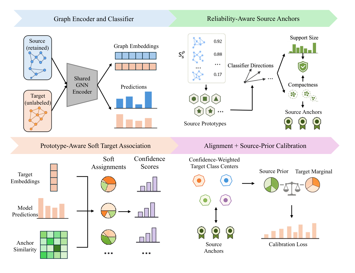
Refer to caption — Figure 1: Overview of the proposed DEAG. DEAG estimates source-class reliability using support size and embedding compactness, constructs reusable source anchors by blending source prototypes with classifier directions, softly associates target graphs with these anchors, and jointly optimizes prototype alignment and source-prior target-marginal calibration.

Graph Domain Adaptation (GDA). GDA transfers predictive knowledge from labeled source graphs to unlabeled target graphs under distribution shifts [46, 3, 6]. Existing GDA methods mainly improve transferability by reducing source-target mismatch in the learned representation space [32, 25, 49]. Representative approaches employ adversarial objectives, distribution alignment, contrastive learning, or variational modeling to learn domain-adaptive graph representations [50, 20]. Since graph data contain both node attributes and relational structures, later studies further incorporate graph-specific inductive biases, including topology-aware regularization, structural reweighting, propagation calibration, and graph-constrained target self-training, to better handle attribute and structural shifts during adaptation [23, 22, 4]. Despite their effectiveness, most existing GDA methods assume that sufficient labeled source graphs are available during training, so that source classifiers, class prototypes, and alignment signals can be estimated reliably [43, 45]. This source-sufficient assumption becomes fragile when the source-data budget is constrained, especially when an adaptive learner must rely on limited retained source evidence for post-deployment adaptation [21]. With fewer source graphs, empirical class prototypes may be biased by sampling noise, target predictions become less reliable, and hard pseudo-labeling or unconstrained alignment can amplify early errors [28, 21, 11]. To address this limitation, DEAG learns reliability-aware source anchors by fusing source prototypes with classifier directions, and uses them for soft target association and source-prior target-marginal calibration, enabling self-guided adaptation under limited source evidence.

3 Methodology

3.1 Problem Formulation

We study data-efficient agentic Graph Domain Adaptation (GDA) under limited retained source evidence. Let $\mathcal{D}_{S}=\{(\mathcal{G}_{i}^{s},y_{i}^{s})\}_{i=1}^{N_{S}}$ be the labeled source domain and $\mathcal{D}_{T}=\{\mathcal{G}_{j}^{t}\}_{j=1}^{N_{T}}$ be the unlabeled target domain, where each graph is $\mathcal{G}=(\mathcal{V},\mathcal{E},\mathbf{X})$ and $y_{i}^{s}\in\mathcal{Y}=\{1,\ldots,C\}$ . Given a source-data ratio $\rho\in(0,1]$ , only a class-stratified retained subset $\mathcal{S}_{S}^{\rho}=\bigcup_{c=1}^{C}\mathcal{S}_{S,c}^{\rho}$ is accessible for training, where $\mathcal{S}_{S,c}^{\rho}\subseteq\mathcal{D}_{S,c}$ , $\mathcal{D}_{S,c}=\{(\mathcal{G}_{i}^{s},y_{i}^{s})\in\mathcal{D}_{S}:y_{i}^{s}=c\}$ , and $|\mathcal{S}_{S,c}^{\rho}|=K_{c}$ . We denote the retained source budget by $K=\sum_{c=1}^{C}K_{c}\ll N_{S}$ .

3.2 Overview of DEAG

Figure 1 illustrates the proposed framework of DEAG. It first extracts graph embeddings with a shared GNN encoder and estimates the reliability of each source class from the retained source subset. To obtain reusable source-side guidance, DEAG blends empirical prototypes with classifier directions according to this reliability, producing reliability-aware source anchors. These anchors then guide the association of unlabeled target observations by combining classifier predictions with target-to-anchor similarities. The resulting soft assignments are confidence-weighted to form target class centers, which are aligned with source anchors without hard pseudo-label training. Finally, a source-prior regularizer calibrates the target marginal using the class prior observed from the retained source evidence.

3.3 Reliability-Aware Source Anchors

Encoder and classifier. We use a standard GNN encoder followed by a linear classifier. For a graph $\mathcal{G}$ , node representations are updated by

\mathbf{H}_{\mathcal{G}}^{(\ell)}=\mathrm{GNN}_{\theta}^{(\ell)}(\mathcal{G},\mathbf{H}_{\mathcal{G}}^{(\ell-1)}),\qquad\mathbf{H}_{\mathcal{G}}^{(0)}=\mathbf{X}.

(1)

The graph representation is obtained as

\mathbf{z}_{\mathcal{G}}=\mathrm{READOUT}\left(\mathbf{H}_{\mathcal{G}}^{(L)}\right)\in\mathbb{R}^{d_{z}},

(2)

and its normalized version is $\widetilde{\mathbf{z}}_{\mathcal{G}}=\mathbf{z}_{\mathcal{G}}/(\|\mathbf{z}_{\mathcal{G}}\|_{2}+\varepsilon)$ , where $\varepsilon>0$ is a numerical constant. The classifier predicts

p_{\theta}(y|\mathcal{G})=\mathrm{softmax}(\mathbf{W}\mathbf{z}_{\mathcal{G}}+\mathbf{b}).

(3)

Let $\mathbf{w}_{c}$ be the classifier weight vector for class $c$ , and define its normalized direction as $\widetilde{\mathbf{w}}_{c}=\mathbf{w}_{c}/(\|\mathbf{w}_{c}\|_{2}+\varepsilon)$ .

Source prototype reliability. Under limited retained source evidence, empirical class prototypes may be noisy and may not provide stable reusable source semantics. For each class $c$ , we compute the retained-source prototype as

\bar{\boldsymbol{\mu}}_{S,c}=\frac{1}{K_{c}}\sum_{(\mathcal{G}_{i}^{s},y_{i}^{s})\in\mathcal{S}_{S,c}^{\rho}}\widetilde{\mathbf{z}}_{\mathcal{G}_{i}^{s}},\qquad\boldsymbol{\mu}_{S,c}=\frac{\bar{\boldsymbol{\mu}}_{S,c}}{\|\bar{\boldsymbol{\mu}}_{S,c}\|_{2}+\varepsilon}.

(4)

We measure prototype compactness by $r_{c}=\|\bar{\boldsymbol{\mu}}_{S,c}\|_{2}$ . Since each normalized embedding has unit norm, $0\leq r_{c}\leq 1$ ; larger $r_{c}$ indicates more concentrated retained source embeddings. We combine compactness with source support size to define the reliability coefficient

\alpha_{c}=\mathrm{sg}\left[\frac{K_{c}-1}{K_{c}}r_{c}\right],

(5)

where $\mathrm{sg}[\cdot]$ denotes stop-gradient. Thus, a class with a single retained source graph obtains $\alpha_{c}=0$ , while a class with sufficient and compact samples obtains a larger reliability score. This coefficient allows the learner to assess how trustworthy the retained source evidence is for each class.

Anchor construction. To balance instance-level source semantics and classifier-level decision geometry, we fuse the empirical prototype with the classifier direction:

\bar{\mathbf{a}}_{c}=\alpha_{c}\boldsymbol{\mu}_{S,c}+(1-\alpha_{c})\widetilde{\mathbf{w}}_{c},\qquad\mathbf{a}_{c}=\mathrm{sg}\left[\frac{\bar{\mathbf{a}}_{c}}{\|\bar{\mathbf{a}}_{c}\|_{2}+\varepsilon}\right].

(6)

The anchor set is $\mathcal{A}_{S}=\{\mathbf{a}_{c}\}_{c=1}^{C}$ . When the prototype is reliable, $\mathbf{a}_{c}$ is dominated by $\boldsymbol{\mu}_{S,c}$ ; otherwise, it falls back to the classifier direction. This prevents noisy prototypes from becoming misleading alignment targets and provides stable reusable source guidance for target adaptation.

3.4 Prototype-Aware Target Association

Since target labels are unavailable, target graphs must be associated with source semantics through predictions and representation similarity. Hard pseudo-labeling is fragile under limited source evidence, so DEAG constructs soft and confidence-weighted target class centers. For target graph $\mathcal{G}_{j}^{t}$ , let $\widetilde{\mathbf{z}}_{j}^{t}=\widetilde{\mathbf{z}}_{\mathcal{G}_{j}^{t}}$ and $p_{j,c}^{t}=p_{\theta}(c|\mathcal{G}_{j}^{t})$ . We define the prototype-aware assignment logit as

\ell_{j,c}=\log(p_{j,c}^{t}+\varepsilon)+(\widetilde{\mathbf{z}}_{j}^{t})^{\top}\mathbf{a}_{c}.

(7)

The first term captures classifier confidence, and the second term measures target-to-anchor compatibility. The detached soft assignment is

q_{j,c}=\mathrm{sg}\left[\frac{\exp(\ell_{j,c})}{\sum_{k=1}^{C}\exp(\ell_{j,k})}\right].

(8)

Here, $q_{j,c}$ is not used as a target pseudo-label for cross-entropy training; it only provides weights for target center estimation. This design allows unlabeled target observations to be cautiously associated with reusable source anchors without committing to hard pseudo-labels.

To suppress ambiguous target graphs, we compute the assignment entropy $H(q_{j})=-\sum_{c=1}^{C}q_{j,c}\log(q_{j,c}+\varepsilon)$ and define

\omega_{j}=\mathrm{sg}\left[1-\frac{H(q_{j})}{\log C}\right].

(9)

For class $c$ , the weighted target mass and detached class weight are

M_{c}=\sum_{j=1}^{N_{T}}\omega_{j}q_{j,c},\qquad\beta_{c}=\mathrm{sg}\left[\frac{M_{c}+\varepsilon}{\sum_{k=1}^{C}M_{k}+C\varepsilon}\right].

(10)

The normalized target center is

\bar{\boldsymbol{\mu}}_{T,c}=\frac{\sum_{j=1}^{N_{T}}\omega_{j}q_{j,c}\widetilde{\mathbf{z}}_{j}^{t}}{M_{c}+\varepsilon},\qquad\boldsymbol{\mu}_{T,c}=\frac{\bar{\boldsymbol{\mu}}_{T,c}}{\|\bar{\boldsymbol{\mu}}_{T,c}\|_{2}+\varepsilon}.

(11)

We align target centers to source anchors by

\mathcal{L}_{pa}=\sum_{c=1}^{C}\beta_{c}\left\|\boldsymbol{\mu}_{T,c}-\mathbf{a}_{c}\right\|_{2}^{2}.

(12)

Gradients are propagated through $\boldsymbol{\mu}_{T,c}$ to update target representations, while $\mathbf{a}_{c}$ , $q_{j,c}$ , $\omega_{j}$ , and $\beta_{c}$ are detached. This avoids degenerate minimization by changing anchors or assignments instead of learning target-aligned representations.

3.5 Source-Prior Target-Marginal Calibration

Prototype alignment transfers reusable class-level source semantics to the target domain, but it may over-concentrate target graphs around a few anchors. To calibrate target predictions before reliable target feedback is available, DEAG introduces a source-prior regularizer. The retained source prior is $\pi_{S,c}=K_{c}/K$ , and the target marginal prediction is $\bar{p}_{T,c}=N_{T}^{-1}\sum_{j=1}^{N_{T}}p_{\theta}(c|\mathcal{G}_{j}^{t})$ . The target conditional entropy is

\mathcal{H}_{cond}=-\frac{1}{N_{T}}\sum_{j=1}^{N_{T}}\sum_{c=1}^{C}p_{\theta}(c|\mathcal{G}_{j}^{t})\log\left(p_{\theta}(c|\mathcal{G}_{j}^{t})+\varepsilon\right),

(13)

and the source-prior matching term is

\mathcal{D}_{prior}=\mathrm{KL}(\pi_{S}\|\bar{p}_{T})=\sum_{c=1}^{C}\pi_{S,c}\log\left(\frac{\pi_{S,c}+\varepsilon}{\bar{p}_{T,c}+\varepsilon}\right).

(14)

The source-prior target regularization loss is $\mathcal{L}_{ptr}=\mathcal{H}_{cond}+\mathcal{D}_{prior}$ . The entropy term sharpens target predictions, while the prior matching term prevents the target marginal from drifting away from retained source evidence. Together, they reduce biased target-marginal updates under limited source evidence and unavailable target labels.

3.6 Overall Learning Objective

The supervised loss is computed only on $\mathcal{S}_{S}^{\rho}$ . To reduce class imbalance under limited retained source evidence, we use class-balanced cross-entropy:

\mathcal{L}_{sup}=\frac{1}{C}\sum_{c=1}^{C}\frac{1}{K_{c}}\sum_{(\mathcal{G}_{i}^{s},y_{i}^{s})\in\mathcal{S}_{S,c}^{\rho}}\mathcal{L}_{CE}\left(p_{\theta}(y|\mathcal{G}_{i}^{s}),c\right).

(15)

The final objective is

\mathcal{L}=\mathcal{L}_{sup}+\lambda_{1}\mathcal{L}_{pa}+\lambda_{2}\mathcal{L}_{ptr},

(16)

where $\lambda_{1},\lambda_{2}\geq 0$ balance the two adaptation losses.

Theorem 3.1 (Target-Risk Bound)

Let $f$ be the graph encoder, $h$ be the classifier, and $g=h\circ f\in\mathcal{H}$ be the learned predictor. Let $\mathcal{R}_{T}(g)$ denote the expected target risk and $\widehat{\mathcal{R}}_{\mathcal{S}_{S}^{\rho}}(g)$ denote the empirical risk on the retained source subset $\mathcal{S}_{S}^{\rho}$ with $K$ samples. For each class $c$ , let $\mathbf{a}_{c}$ be the learned reliability-aware source anchor and $\mathbf{a}_{c}^{\star}$ be the ideal class anchor estimated with sufficient source support. Define the retained-source prior $\pi_{S,c}=K_{c}/K$ , the anchor estimation error $\epsilon_{\mathrm{anc}}=\sum_{c=1}^{C}\pi_{S,c}\|\mathbf{a}_{c}-\mathbf{a}_{c}^{\star}\|_{2}$ , and the class-mass factor $\gamma_{\beta}=\sum_{c=1}^{C}\pi_{S,c}^{2}/\beta_{c}$ , where $\beta_{c}>0$ is the detached target class-mass weight in $\mathcal{L}_{pa}$ . Assume the loss $\ell$ is bounded in $[0,1]$ and $K_{\mathrm{Lip}}$ -Lipschitz with respect to normalized graph representations. Then, with probability at least $1-\delta$ , the target risk is bounded by

	$\displaystyle\mathcal{R}_{T}(g)\leq$	$\displaystyle\widehat{\mathcal{R}}_{\mathcal{S}_{S}^{\rho}}(g)+K_{\mathrm{Lip}}\sqrt{\gamma_{\beta}\mathcal{L}_{pa}}+\sqrt{2\mathcal{D}_{prior}}+K_{\mathrm{Lip}}\epsilon_{\mathrm{anc}}$		(17)
		$\displaystyle+2\mathfrak{R}_{K}(\mathcal{H})+3\sqrt{\frac{\log(2/\delta)}{2K}}+\lambda^{\star},$		(17)

where $\mathfrak{R}_{K}(\mathcal{H})$ is the empirical Rademacher complexity of $\mathcal{H}$ under $K$ retained source samples, and $\lambda^{\star}$ denotes the minimal joint risk and residual mismatch between the retained source and target domains.

Theorem 3.1 shows that DEAG controls target risk through three optimizable terms. The prototype alignment loss $\mathcal{L}_{pa}$ reduces class-wise representation discrepancy, the prior matching term $\mathcal{D}_{prior}$ controls target marginal mismatch, and the reliability-aware anchor construction reduces $\epsilon_{\mathrm{anc}}$ by preventing noisy empirical prototypes from dominating target alignment. The proof of Theorem 3.1 can be found in Appendix 0.A.

4 Experiments

4.1 Experimental Settings

Datasets. We evaluate DEAG on two representative types of graph distribution shifts. (1) Structure-based domain shifts are constructed on Mutagenicity [17] and NCI1 [30]. Following standard GDA protocols [43, 44], we partition graphs by node-density and edge-density statistics to create source and target domains with different structural biases while preserving the original classification tasks. (2) Feature-based domain shifts are evaluated on commonly used paired benchmarks, including DD, PROTEINS, BZR, BZR_MD, COX2, and COX2_MD, where source and target domains exhibit notable feature distribution discrepancies. The statistics of the above datasets are provided in Appendix 0.B.

Baselines. We compare DEAG with three groups of baselines. The first group contains the graph kernel method PathNN [26]. The second group includes four general GNN backbones: GCN [18], GIN [41], CIN [2], and GMT [1]. The third group includes seven representative GDA methods: DEAL [43], SGDA [28], StruRW [23], A2GNN [22], PA-BOTH [24], GAA [7], and TDSS [4].

Implementation Details. We implement DEAG in PyTorch. Unless otherwise specified, GIN [41] is used as the backbone encoder, with three GNN layers and a hidden dimension of 128. All neural methods are optimized with Adam using a learning rate of $3\times 10^{-4}$ and a weight decay of $1\times 10^{-12}$ . We use a class-stratified retained source subset with source-data ratio $\rho=0.3$ by default. For DEAG, the loss coefficients are fixed to $\lambda_{1}=0.7$ and $\lambda_{2}=0.5$ . We report classification accuracy as the evaluation metric, and present the mean and standard deviation over five independent runs.

Table 1: Graph classification results (in %) under node and edge density domain shifts on the Mutagenicity dataset, and under feature shifts (source

\rightarrow

target). P, D, C, CM, B, and BM denote PROTEINS, DD, COX2, COX2_MD, BZR, and BZR_MD, respectively. Bold indicates the best performance.

Methods	Node Shift			Edge Shift			Feature Shift
Methods	M0 $\rightarrow$ M1	M0 $\rightarrow$ M2	M0 $\rightarrow$ M3	M0 $\rightarrow$ M1	M0 $\rightarrow$ M2	M0 $\rightarrow$ M3	P $\rightarrow$ D	D $\rightarrow$ P	C $\rightarrow$ CM	CM $\rightarrow$ C	B $\rightarrow$ BM	BM $\rightarrow$ B
GCN	53.2 $\pm$ 4.1	49.5 $\pm$ 3.6	50.1 $\pm$ 4.5	61.5 $\pm$ 5.4	53.2 $\pm$ 4.8	47.3 $\pm$ 3.2	52.3 $\pm$ 4.1	48.7 $\pm$ 5.2	41.2 $\pm$ 3.8	45.6 $\pm$ 2.9	44.3 $\pm$ 6.2	43.8 $\pm$ 4.7
GIN	51.4 $\pm$ 5.2	47.8 $\pm$ 4.4	49.6 $\pm$ 3.8	59.8 $\pm$ 6.1	51.6 $\pm$ 5.2	46.5 $\pm$ 4.1	50.7 $\pm$ 5.3	47.2 $\pm$ 4.6	40.8 $\pm$ 4.1	44.9 $\pm$ 3.2	43.6 $\pm$ 5.8	42.1 $\pm$ 4.9
GMT	55.1 $\pm$ 3.8	51.2 $\pm$ 3.2	51.5 $\pm$ 2.9	62.4 $\pm$ 4.5	54.5 $\pm$ 3.9	48.2 $\pm$ 2.8	54.2 $\pm$ 3.7	49.6 $\pm$ 3.4	42.4 $\pm$ 3.6	46.8 $\pm$ 2.8	45.4 $\pm$ 5.1	44.7 $\pm$ 4.2
CIN	54.3 $\pm$ 4.5	50.6 $\pm$ 3.7	50.9 $\pm$ 3.4	61.9 $\pm$ 5.0	53.8 $\pm$ 4.2	47.8 $\pm$ 3.1	53.6 $\pm$ 4.2	48.9 $\pm$ 4.1	41.7 $\pm$ 3.9	45.2 $\pm$ 3.1	44.8 $\pm$ 5.4	43.9 $\pm$ 4.5
PathNN	52.8 $\pm$ 4.8	48.9 $\pm$ 4.1	50.4 $\pm$ 3.6	60.5 $\pm$ 5.6	52.4 $\pm$ 4.9	46.9 $\pm$ 3.7	51.8 $\pm$ 4.6	47.8 $\pm$ 4.3	41.1 $\pm$ 4.2	44.7 $\pm$ 3.4	43.9 $\pm$ 5.6	43.2 $\pm$ 4.8
DEAL	72.1 $\pm$ 2.1	64.8 $\pm$ 2.4	56.1 $\pm$ 1.2	72.8 $\pm$ 0.7	62.5 $\pm$ 2.1	54.2 $\pm$ 1.4	59.8 $\pm$ 0.9	50.2 $\pm$ 9.8	42.1 $\pm$ 6.1	49.3 $\pm$ 3.5	48.9 $\pm$ 7.6	47.7 $\pm$ 5.0
SGDA	54.7 $\pm$ 4.6	50.2 $\pm$ 3.7	50.8 $\pm$ 4.1	63.3 $\pm$ 6.9	54.1 $\pm$ 5.7	47.9 $\pm$ 4.1	48.0 $\pm$ 3.8	54.6 $\pm$ 10.8	41.3 $\pm$ 0.3	49.8 $\pm$ 1.5	49.8 $\pm$ 9.9	51.7 $\pm$ 8.5
A2GNN	42.5 $\pm$ 7.1	46.1 $\pm$ 6.5	50.6 $\pm$ 3.8	60.6 $\pm$ 8.7	54.4 $\pm$ 7.2	49.1 $\pm$ 3.5	61.9 $\pm$ 0.7	57.0 $\pm$ 1.0	45.4 $\pm$ 9.9	45.5 $\pm$ 5.4	48.1 $\pm$ 5.3	63.0 $\pm$ 4.4
StruRW	74.3 $\pm$ 1.7	66.8 $\pm$ 1.1	53.2 $\pm$ 1.8	73.1 $\pm$ 0.9	63.7 $\pm$ 1.6	50.8 $\pm$ 2.1	54.0 $\pm$ 6.9	47.6 $\pm$ 11.4	40.7 $\pm$ 0.2	49.5 $\pm$ 2.8	48.8 $\pm$ 8.0	52.3 $\pm$ 4.8
PA-BOTH	72.9 $\pm$ 0.8	65.4 $\pm$ 2.3	52.1 $\pm$ 0.9	72.4 $\pm$ 1.1	53.9 $\pm$ 6.2	52.5 $\pm$ 1.4	54.1 $\pm$ 6.4	47.1 $\pm$ 10.0	40.7 $\pm$ 0.2	49.8 $\pm$ 2.6	49.9 $\pm$ 7.0	51.4 $\pm$ 4.9
GAA	75.8 $\pm$ 1.4	68.9 $\pm$ 0.9	55.5 $\pm$ 1.1	72.9 $\pm$ 1.2	65.7 $\pm$ 1.1	55.5 $\pm$ 2.3	47.0 $\pm$ 3.7	58.0 $\pm$ 1.8	53.0 $\pm$ 12.8	50.1 $\pm$ 3.3	52.0 $\pm$ 6.8	49.4 $\pm$ 9.7
TDSS	43.8 $\pm$ 6.6	50.1 $\pm$ 7.1	50.9 $\pm$ 3.2	62.6 $\pm$ 8.5	54.0 $\pm$ 5.9	49.4 $\pm$ 4.6	62.3 $\pm$ 0.6	57.9 $\pm$ 0.5	45.4 $\pm$ 9.9	46.5 $\pm$ 3.3	46.6 $\pm$ 6.9	50.5 $\pm$ 24.1
DEAG	76.9 $\pm$ 2.2	69.7 $\pm$ 1.2	63.4 $\pm$ 2.3	74.8 $\pm$ 1.2	67.1 $\pm$ 1.6	65.6 $\pm$ 2.3	64.1 $\pm$ 1.5	62.5 $\pm$ 3.1	54.2 $\pm$ 11.8	51.3 $\pm$ 4.5	53.1 $\pm$ 9.5	68.3 $\pm$ 8.8

Table 2: Aggregate comparison across all reported tasks. Bold results indicate the best performance.

Methods	Node Avg.	Edge Avg.	Feature Avg.	Avg. Rank	$p$ -value	W/T/L
GCN	46.82	47.23	45.98	11.52	$1.84{\times}10^{-23}$	54/0/0
GIN	46.25	46.87	44.88	12.34	$1.23{\times}10^{-23}$	54/0/0
GMT	48.03	48.46	47.18	7.78	$4.25{\times}10^{-22}$	54/0/0
CIN	47.50	47.89	46.35	9.91	$8.96{\times}10^{-23}$	54/0/0
PathNN	47.08	47.52	45.42	10.13	$4.90{\times}10^{-23}$	54/0/0
DEAL	57.10	56.87	49.67	3.75	$3.38{\times}10^{-15}$	52/1/1
SGDA	48.30	49.45	49.20	6.88	$4.71{\times}10^{-21}$	53/0/1
A2GNN	48.27	48.77	53.48	6.88	$2.62{\times}10^{-19}$	54/0/0
StruRW	52.08	52.85	48.82	5.86	$6.12{\times}10^{-16}$	53/0/1
PA-BOTH	52.63	52.54	48.83	5.69	$1.37{\times}10^{-15}$	53/0/1
GAA	63.15	62.20	51.58	2.49	$2.58{\times}10^{-8}$	48/1/5
TDSS	48.60	48.96	51.53	6.55	$4.54{\times}10^{-19}$	52/0/2
DEAG	66.89	66.45	58.92	1.22	–	–

4.2 Performance Comparison

Table 1, 5-8 report the performance comparison under different domain shifts. From these tables, we can make the following observations: (1) Standard GNNs such as GCN, GIN, and GMT generally perform poorly under domain shifts, indicating that directly transferring a predictor trained on the retained source subset is insufficient when target graphs exhibit shifted structures or features. Since these methods do not exploit unlabeled target observations, their predictions are sensitive to reduced and potentially biased source evidence. (2) Existing GDA methods, including DEAL, GAA, and TDSS, usually improve over standard graph classifiers, confirming the benefit of adaptation objectives under source-target shifts. By leveraging representation alignment, propagation calibration, structural reweighting, target-side smoothing, or attribute-based adaptation, they can partially reduce domain discrepancy. However, their performance remains unstable across shift types and transfer directions, suggesting that existing GDA objectives still depend on reliable source semantics, which become fragile when only limited source graphs are retained. (3) DEAG achieves the best average performance and the lowest average rank, demonstrating its effectiveness for data-efficient agentic GDA. The gains mainly come from reliability-aware source anchors, which combine empirical prototypes with classifier directions to stabilize reusable source guidance under limited retained evidence. Moreover, prototype-aware soft target association aligns confidence-weighted target centers with source anchors, enabling unlabeled target observations to be associated with source semantics without hard pseudo-labels. Source-prior regularization further calibrates the target marginal by encouraging confident predictions while preventing drift toward unreliable classes. More results on other datasets can be found in Appendix 0.C.

To summarize performance across all shift types, we report aggregate results in Table 2. Node Avg., Edge Avg., and Feature Avg. denote the mean accuracy over node-density, edge-density, and feature-shift tasks, respectively. Avg. Rank is computed over all $54$ reported settings, where a smaller value indicates better overall performance. The $p$ -value is obtained by a paired task-level $t$ -test between DEAG and each baseline, and W/T/L counts the number of wins, ties, and losses according to the reported mean $\pm$ standard-deviation intervals. As shown in Table 2, DEAG achieves the best average performance across all three shift categories and obtains the lowest Avg. Rank of $1.22$ . Compared with the strongest baseline GAA, DEAG still achieves a clear advantage, with $48$ wins over $54$ settings. These results indicate that the improvement of DEAG is consistent across different shift types rather than being driven by a few favorable tasks, suggesting higher information yield from the same retained source budget.

4.3 Information Yield under Source-Data Budgets

To evaluate how effectively each method exploits retained source evidence, we vary the source-data ratio $\rho$ within $\{0.1,0.3,0.5,0.7,0.9\}$ on Mutagenicity node shift and report the average accuracy in Figure 2(a). We compare DEAG with two strong GDA baselines, GAA and DEAL, as well as the average performance of all compared baselines.

As shown in Figure 2(a), DEAG outperforms both strong baselines and the average baseline across all source ratios. The advantage is particularly evident when the retained source ratio is small, where existing GDA methods suffer from weaker source supervision and less reliable alignment signals. By estimating reliability-aware anchors from the retained subset and using them to guide soft target association, DEAG extracts more useful adaptation signals from limited source evidence. As the source ratio increases, all methods benefit from additional source graphs, but DEAG maintains a clear margin, demonstrating that the proposed framework improves adaptation effectiveness under the same source-data budget.

(a) Source data ratio

\rho

(b)

\lambda_{1}

(c)

\lambda_{2}

Figure 2: Information yield under source-data budgets and sensitivity analysis on Mutagenicity.

4.4 Sensitivity Analysis

We analyze the sensitivity of DEAG to the two balancing coefficients $\lambda_{1}$ and $\lambda_{2}$ . The coefficient $\lambda_{1}$ controls the prototype alignment loss $\mathcal{L}_{pa}$ , while $\lambda_{2}$ controls the source-prior target regularization loss $\mathcal{L}_{ptr}$ . We vary each coefficient within $\{0.1,0.3,0.5,0.7,0.9\}$ and keep the other hyperparameters fixed.

Figures 2(b)(c) show that DEAG is stable across a broad range of both coefficients. A small $\lambda_{1}$ provides insufficient guidance from reliability-aware source anchors, while a moderate value strengthens class-level semantic transfer. An overly large $\lambda_{1}$ can slightly reduce flexibility by forcing uncertain target centers toward imperfect anchors. For $\lambda_{2}$ , a small value weakens target-marginal calibration and makes predictions more prone to drifting toward initially favored classes. A moderate value improves robustness by jointly sharpening target predictions and matching the target marginal to the retained source prior, whereas an excessively large value may over-constrain the target distribution. The default setting $\lambda_{1}=0.7$ and $\lambda_{2}=0.5$ provides a good balance between source-semantic alignment and target-marginal calibration.

4.5 Ablation Study

We conduct ablation studies to examine the contribution of each component in DEAG. DEAG w/o $\mathcal{L}_{pa}$ removes the prototype alignment loss, so target centers are no longer explicitly aligned with reliability-aware source anchors. DEAG w/o $\mathcal{L}_{ptr}$ removes the source-prior target regularization loss. To further disentangle $\mathcal{L}_{ptr}$ , DEAG w/o $H_{\mathrm{cond}}$ removes the conditional entropy term, while DEAG w/o $D_{\mathrm{prior}}$ removes the source-prior matching term.

Table 3: The results of ablation studies on the Mutagenicity dataset. Bold results indicate the best performance.

Method	M0 $\rightarrow$ M1	M0 $\rightarrow$ M2	M0 $\rightarrow$ M3	M1 $\rightarrow$ M0	M1 $\rightarrow$ M2	M1 $\rightarrow$ M3	M2 $\rightarrow$ M0	M2 $\rightarrow$ M1	M2 $\rightarrow$ M3	M3 $\rightarrow$ M0	M3 $\rightarrow$ M1	M3 $\rightarrow$ M2
DEAG w/o $\mathcal{L}_{pa}$	70.8	63.4	57.1	65.4	67.5	59.8	62.3	73.1	61.2	58.6	60.1	67.8
DEAG w/o $\mathcal{L}_{ptr}$	73.4	66.1	60.3	67.3	70.2	62.5	65.0	75.8	64.1	62.1	63.4	70.6
DEAG w/o $H_{\text{cond}}$	74.9	67.5	61.6	69.8	71.8	64.1	66.9	77.4	65.7	63.4	65.0	72.3
DEAG w/o $D_{\text{prior}}$	75.3	68.2	61.2	70.7	72.3	64.6	67.8	77.8	66.2	63.1	65.5	72.7
DEAG	76.9	69.7	63.4	71.8	73.7	65.9	69.1	79.2	67.5	65.0	66.8	74.0

Table 3 reports the ablation results. From the table, we make four observations: (1) The full model achieves the best performance across the ablation settings, indicating that the three components of DEAG provide complementary benefits rather than redundant regularization. (2) Removing $\mathcal{L}_{pa}$ leads to the most consistent and pronounced degradation. This trend shows that reliability-aware prototype alignment is the primary mechanism for transferring reusable class-level source semantics to the target domain. Without this loss, target representations are no longer explicitly guided toward source anchors, making adaptation more vulnerable to weakened source evidence. (3) Removing $\mathcal{L}_{ptr}$ also causes clear performance drops across transfer directions, suggesting that prototype alignment alone cannot fully stabilize target predictions. This confirms the necessity of source-prior target regularization, especially when early target associations may be biased under limited source evidence. (4) Removing either $H_{\mathrm{cond}}$ or $D_{\mathrm{prior}}$ weakens the model, but the degradation is generally milder than removing the entire $\mathcal{L}_{ptr}$ . This indicates that the two terms play complementary roles: $H_{\mathrm{cond}}$ improves sample-level prediction confidence, while $D_{\mathrm{prior}}$ constrains the target marginal using retained source evidence. Overall, the ablation trends verify that DEAG benefits from the joint effect of reliability-aware source anchoring, prototype-aware target association, and source-prior target-marginal calibration in the limited-source setting.

5 Conclusion

We propose DEAG, a reliability-aware prototype learning framework for data-efficient agentic graph domain adaptation. Using source support and embedding compactness, DEAG blends empirical prototypes with classifier directions into reusable anchors. Soft association aligns confidence-weighted target centers with these anchors without hard pseudo-label training, while source-prior marginal calibration stabilizes predictions using retained source evidence. Experiments across structural and feature shifts demonstrate average gains over competitive baselines under matched source-data budgets.

References

[1] J. Baek, M. Kang, and S. J. Hwang (2021) Accurate learning of graph representations with graph multiset pooling. arXiv preprint arXiv:2102.11533. Cited by: §4.1.
[2] C. Bodnar, F. Frasca, N. Otter, Y. Wang, P. Lio, G. F. Montufar, and M. Bronstein (2021) Weisfeiler and lehman go cellular: cw networks. Proceedings of the Conference on Neural Information Processing Systems. Cited by: §4.1.
[3] R. Cai, F. Wu, Z. Li, P. Wei, L. Yi, and K. Zhang (2024) Graph domain adaptation: a generative view. ACM Transactions on Knowledge Discovery from Data. Cited by: §2.
[4] W. Chen, G. Ye, Y. Wang, Z. Zhang, L. Zhang, D. Wang, Z. Zhang, and F. Zhuang (2025) Smoothness really matters: a simple yet effective approach for unsupervised graph domain adaptation. In Proceedings of the AAAI Conference on Artificial Intelligence, Cited by: §1, §2, §4.1.
[5] B. G. Collaco, S. A. Haider, S. Prabha, C. A. Gomez-Cabello, A. Genovese, N. G. Wood, S. P. Bagaria, N. Gopala, C. Tao, and A. J. Forte (2026) The role of agentic artificial intelligence in healthcare: a scoping review. npj Digital Medicine. Cited by: §1.
[6] Q. Dai, X. Wu, J. Xiao, X. Shen, and D. Wang (2022) Graph transfer learning via adversarial domain adaptation with graph convolution. IEEE Transactions on Knowledge and Data Engineering. Cited by: §2.
[7] R. Fang, B. Li, Q. Zeng, N. Hosseini Dashtbayaz, R. Pu, C. Ling, B. Wang, et al. (2025) On the benefits of attribute-driven graph domain adaptation. In Proceedings of the International Conference on Learning Representations, Cited by: §4.1.
[8] R. Fang, B. Li, J. Zhao, R. Pu, Q. Zeng, G. Xu, C. Ling, and B. Wang (2025) Homophily enhanced graph domain adaptation. arXiv preprint arXiv:2505.20089. Cited by: §1.
[9] Y. Ganin, E. Ustinova, H. Ajakan, P. Germain, H. Larochelle, F. Laviolette, M. March, and V. Lempitsky (2016) Domain-adversarial training of neural networks. The Journal of Machine Learning Research.. Cited by: §1.
[10] X. Gao, J. Yu, T. Chen, G. Ye, W. Zhang, and H. Yin (2025) Graph condensation: a survey. IEEE Transactions on Knowledge and Data Engineering. Cited by: §2.
[11] S. Garg, N. Erickson, J. Sharpnack, A. Smola, S. Balakrishnan, and Z. C. Lipton (2023) Rlsbench: domain adaptation under relaxed label shift. In Proceedings of the International Conference on Machine Learning, Cited by: §1, §2, §2.
[12] H. Hadipour, Y. Y. Li, Y. Sun, C. Deng, L. Lac, R. Davis, S. T. Cardona, and P. Hu (2025) GraphBAN: an inductive graph-based approach for enhanced prediction of compound-protein interactions. Nature Communications. Cited by: §1.
[13] M. Hashemi, S. Gong, J. Ni, W. Fan, B. A. Prakash, and W. Jin (2024) A comprehensive survey on graph reduction: sparsification, coarsening, and condensation. arXiv preprint arXiv:2402.03358. Cited by: §2.
[14] S. Hu, C. Lu, and J. Clune (2025) Automated design of agentic systems. In Proceedings of the International Conference on Learning Representations, Cited by: §1.
[15] S. Hu, G. Zou, S. Yang, S. Lin, Y. Gan, B. Zhang, and Y. Chen (2025) Large language model meets graph neural network in knowledge distillation. In Proceedings of the AAAI Conference on Artificial Intelligence, Cited by: §2.
[16] W. Ju, S. Yi, Y. Wang, Q. Long, J. Luo, Z. Xiao, and M. Zhang (2024) A survey of data-efficient graph learning. arXiv preprint arXiv:2402.00447. Cited by: §2.
[17] J. Kazius, R. McGuire, and R. Bursi (2005) Derivation and validation of toxicophores for mutagenicity prediction. Journal of medicinal chemistry. Cited by: §4.1.
[18] T. N. Kipf and M. Welling (2016) Semi-supervised classification with graph convolutional networks. arXiv preprint arXiv:1609.02907. Cited by: §1, §4.1.
[19] P. I. Lei, X. Chen, Y. Sheng, Y. Liu, Z. Gong, and Q. Yang (2025) Gradual domain adaptation for graph learning. ACM Transactions on Intelligent Systems and Technology. Cited by: §1.
[20] W. Li, X. Liu, and Y. Yuan (2023) Sigma++: improved semantic-complete graph matching for domain adaptive object detection. IEEE Transactions on Pattern Analysis and Machine Intelligence 45 (7), pp. 9022–9040. Cited by: §2.
[21] J. Liang, D. Hu, and J. Feng (2020) Do we really need to access the source data? source hypothesis transfer for unsupervised domain adaptation. In Proceedings of the International Conference on Machine Learning, Cited by: §1, §1, §2, §2.
[22] M. Liu, Z. Fang, Z. Zhang, M. Gu, S. Zhou, X. Wang, and J. Bu (2024) Rethinking propagation for unsupervised graph domain adaptation. In Proceedings of the AAAI Conference on Artificial Intelligence, Cited by: §1, §1, §2, §4.1.
[23] S. Liu, T. Li, Y. Feng, N. Tran, H. Zhao, Q. Qiu, and P. Li (2023) Structural re-weighting improves graph domain adaptation. In Proceedings of the International Conference on Machine Learning, Cited by: §1, §2, §4.1.
[24] S. Liu, D. Zou, H. Zhao, and P. Li (2024) Pairwise alignment improves graph domain adaptation. arXiv preprint arXiv:2403.01092. Cited by: §1, §4.1.
[25] M. Long, Y. Cao, J. Wang, and M. Jordan (2015) Learning transferable features with deep adaptation networks. In Proceedings of the International Conference on Machine Learning, Cited by: §1, §2.
[26] G. Michel, G. Nikolentzos, J. F. Lutzeyer, and M. Vazirgiannis (2023) Path neural networks: expressive and accurate graph neural networks. In Proceedings of the International Conference on Machine Learning, Cited by: §4.1.
[27] B. H. Ngo, D. C. Bui, N. Do-Tran, and T. J. Choi (2025) Higda: hierarchical graph of nodes to learn local-to-global topology for semi-supervised domain adaptation. In Proceedings of the AAAI Conference on Artificial Intelligence, Cited by: §1, §2.
[28] Z. Qiao, X. Luo, M. Xiao, H. Dong, Y. Zhou, and H. Xiong (2023) Semi-supervised domain adaptation in graph transfer learning. arXiv preprint arXiv:2309.10773. Cited by: §1, §1, §2, §4.1.
[29] Y. Tian, S. Pei, X. Zhang, C. Zhang, and N. V. Chawla (2025) Knowledge distillation on graphs: a survey. ACM Computing Surveys. Cited by: §2.
[30] N. Wale, I. A. Watson, and G. Karypis (2008) Comparison of descriptor spaces for chemical compound retrieval and classification. Knowledge and Information Systems. Cited by: §4.1.
[31] J. Wang, X. Zheng, Y. Li, and Y. Guo (2025) Correction to: domain graph-structured multi-source domain adaptation with dual integration. In International Conference on Advanced Data Mining and Applications, Cited by: §1.
[32] Y. Wang, T. Zhao, Z. Wu, and S. Wang (2025) Bridging source and target domains via link prediction for unsupervised domain adaptation on graphs. In Proceedings of the International ACM Conference on Web Search & Data Mining, Cited by: §2.
[33] Y. Wang, H. Huang, Z. Zheng, and S. Liang (2026) Cross-resolution semantic learning for graph domain adaptation. arXiv preprint arXiv:2607.29365. Cited by: §1.
[34] Y. Wang, V. Liang, N. Yin, S. Liu, and E. Segal (2026) SGAC: a graph neural network framework for imbalanced and structure-aware amp classification. Briefings in Bioinformatics 27 (1), pp. bbag038. Cited by: §1.
[35] Y. Wang, X. Liu, M. Wang, S. Gao, and N. Yin (2026) DisRFM: polar riemannian flow matching for structure-preserving graph domain adaptation. arXiv preprint arXiv:2602.00656. Cited by: §1.
[36] Y. Wang, M. Wang, Z. Huang, S. Liu, and N. Yin (2026) Nested graph pseudo-label refinement for noisy label domain adaptation learning. In Proceedings of the AAAI Conference on Artificial Intelligence, Cited by: §1.
[37] Y. Wang, M. Wang, H. Su, N. Yin, Q. Yao, and J. Kwok (2024) Degree-conscious spiking graph for cross-domain adaptation. arXiv preprint arXiv:2410.06883. Cited by: §1.
[38] Y. Wang, N. Yin, M. Xiao, X. Yi, S. Liu, and S. Liang (2025) Dusego: dual second-order equivariant graph ordinary differential equation. ACM Transactions on Knowledge Discovery from Data 20 (1), pp. 1–18. Cited by: §1.
[39] Y. Wang, K. Zhang, J. Huang, N. Yin, S. Liu, and E. Segal (2025) Protomol: enhancing molecular property prediction via prototype-guided multimodal learning. Briefings in Bioinformatics 26 (6), pp. bbaf629. Cited by: §1.
[40] Y. Wang, K. Zhang, M. Wang, S. Gao, and N. Yin (2026) Usbd: universal structural basis distillation for source-free graph domain adaptation. arXiv preprint arXiv:2602.08431. Cited by: §2.
[41] K. Xu, W. Hu, J. Leskovec, and S. Jegelka (2018) How powerful are graph neural networks?. arXiv preprint arXiv:1810.00826. Cited by: §1, §4.1, §4.1.
[42] Z. Yang, J. Han, C. Wang, and H. Liu (2025) Graphlora: structure-aware contrastive low-rank adaptation for cross-graph transfer learning. In Proceedings of the International ACM SIGKDD Conference on Knowledge Discovery & Data Mining, Cited by: §1.
[43] N. Yin, L. Shen, B. Li, M. Wang, X. Luo, C. Chen, Z. Luo, and X. Hua (2022) Deal: an unsupervised domain adaptive framework for graph-level classification. In Proceedings of the ACM International Conference on Multimedia, Cited by: §1, §1, §2, §4.1, §4.1.
[44] N. Yin, L. Shen, M. Wang, L. Lan, Z. Ma, C. Chen, X. Hua, and X. Luo (2023) Coco: a coupled contrastive framework for unsupervised domain adaptive graph classification. In Proceedings of the International Conference on Machine Learning, Cited by: §1, §1, §2, §4.1.
[45] N. Yin, L. Shen, M. Wang, X. Liu, C. Chen, and X. Hua (2025) Dream: a dual variational framework for unsupervised graph domain adaptation. IEEE Transactions on Pattern Analysis and Machine Intelligence. Cited by: §1, §1, §2, §2.
[46] Y. You, T. Chen, Z. Wang, and Y. Shen (2023) Graph domain adaptation via theory-grounded spectral regularization. In Proceedings of the International Conference on Learning Representations, Cited by: §2.
[47] X. Yu, Z. Gong, C. Zhou, Y. Fang, and H. Zhang (2025) Samgpt: text-free graph foundation model for multi-domain pre-training and cross-domain adaptation. In Proceedings of the ACM Web Conference, Cited by: §2.
[48] Z. Zeng, R. Qiu, W. Bao, T. Wei, X. Lin, Y. Yan, T. F. Abdelzaher, J. Han, and H. Tong (2025) Pave your own path: graph gradual domain adaptation on fused gromov-wasserstein geodesics. arXiv preprint arXiv:2505.12709. Cited by: §1.
[49] C. Zhang, F. Nie, and R. Wang (2024) Anchor guided unsupervised domain adaptation. IEEE Transactions on Knowledge and Data Engineering. Cited by: §2.
[50] K. Zhang, S. Liu, S. Wang, W. Shi, C. Chen, P. Li, S. Li, J. Li, and K. Ding (2026) A survey of deep graph learning under distribution shifts: from graph out-of-distribution generalization to adaptation. ACM Transactions on Knowledge Discovery from Data. Cited by: §2.
[51] K. Zhang and T. Xu (2026) BrainRiem: riemannian prototype learning for source-free cross-site brain network diagnosis. arXiv preprint arXiv:2606.29200. Cited by: §1.
[52] Y. Zhang, T. Zhang, K. Wang, Z. Guo, Y. Liang, X. Bresson, W. Jin, and Y. You (2024) Navigating complexity: toward lossless graph condensation via expanding window matching. arXiv preprint arXiv:2402.05011. Cited by: §2.

Appendix 0.A Proof of Theorem 3.1

Theorem 3.1 (Target-Risk Bound) Let $f$ be the graph encoder, $h$ be the classifier, and $g=h\circ f\in\mathcal{H}$ be the learned predictor. Let $\mathcal{R}_{T}(g)$ denote the expected target risk and $\widehat{\mathcal{R}}_{\mathcal{S}_{S}^{\rho}}(g)$ denote the empirical risk on the retained source subset $\mathcal{S}_{S}^{\rho}$ with $K$ samples. For each class $c$ , let $\mathbf{a}_{c}$ be the learned reliability-aware source anchor and $\mathbf{a}_{c}^{\star}$ be the ideal class anchor estimated with sufficient source support. Define the retained-source prior $\pi_{S,c}=K_{c}/K$ , the anchor estimation error $\epsilon_{\mathrm{anc}}=\sum_{c=1}^{C}\pi_{S,c}\|\mathbf{a}_{c}-\mathbf{a}_{c}^{\star}\|_{2}$ , and the class-mass factor $\gamma_{\beta}=\sum_{c=1}^{C}\pi_{S,c}^{2}/\beta_{c}$ , where $\beta_{c}>0$ is the detached target class-mass weight in $\mathcal{L}_{pa}$ . Assume the loss $\ell$ is bounded in $[0,1]$ and $K_{\mathrm{Lip}}$ -Lipschitz with respect to normalized graph representations. Then, with probability at least $1-\delta$ , the target risk is bounded by

	$\displaystyle\mathcal{R}_{T}(g)\leq$	$\displaystyle\widehat{\mathcal{R}}_{\mathcal{S}_{S}^{\rho}}(g)+K_{\mathrm{Lip}}\sqrt{\gamma_{\beta}\mathcal{L}_{pa}}+\sqrt{2\mathcal{D}_{prior}}+K_{\mathrm{Lip}}\epsilon_{\mathrm{anc}}$		(18)
		$\displaystyle+2\mathfrak{R}_{K}(\mathcal{H})+3\sqrt{\frac{\log(2/\delta)}{2K}}+\lambda^{\star},$		(18)

Proof

Let $g=h\circ f$ denote the learned predictor. We use $\mathcal{P}_{S}^{\rho}$ to denote the retained-source distribution induced by $\mathcal{S}_{S}^{\rho}$ , and $\mathcal{P}_{T}$ to denote the target distribution. The expected risks on the retained-source and target domains are denoted by $\mathcal{R}_{S}^{\rho}(g)$ and $\mathcal{R}_{T}(g)$ , respectively.

Since the loss $\ell$ is bounded in $[0,1]$ , the standard Rademacher generalization inequality implies that, with probability at least $1-\delta$ ,

\mathcal{R}_{S}^{\rho}(g)\leq\widehat{\mathcal{R}}_{\mathcal{S}_{S}^{\rho}}(g)+2\mathfrak{R}_{K}(\mathcal{H})+3\sqrt{\frac{\log(2/\delta)}{2K}},

(19)

where $\mathfrak{R}_{K}(\mathcal{H})$ is the empirical Rademacher complexity of $\mathcal{H}$ under $K$ retained source samples.

We next relate the retained-source risk to the target risk. Following the standard domain adaptation decomposition, the target risk can be upper bounded by the retained-source risk, a class-conditional representation discrepancy, a marginal-prior discrepancy, and an irreducible residual term:

\mathcal{R}_{T}(g)\leq\mathcal{R}_{S}^{\rho}(g)+\Delta_{\mathrm{cls}}(g)+\Delta_{\mathrm{prior}}(g)+\lambda^{\star},

(20)

where $\lambda^{\star}$ denotes the minimal joint risk and residual mismatch between the retained-source and target domains.

We first bound the class-conditional discrepancy $\Delta_{\mathrm{cls}}(g)$ . For each class $c$ , let $\boldsymbol{\mu}_{T,c}$ denote the confidence-weighted target center, $\mathbf{a}_{c}$ denote the learned reliability-aware source anchor, and $\mathbf{a}_{c}^{\star}$ denote the ideal source anchor obtained with sufficient source support. Since the loss is $K_{\mathrm{Lip}}$ -Lipschitz with respect to normalized graph representations, the discrepancy between the target class center and the ideal source class anchor satisfies

\Delta_{\mathrm{cls}}(g)\leq K_{\mathrm{Lip}}\sum_{c=1}^{C}\pi_{S,c}\left\|\boldsymbol{\mu}_{T,c}-\mathbf{a}_{c}^{\star}\right\|_{2}.

(21)

By the triangle inequality, for every class $c$ ,

\left\|\boldsymbol{\mu}_{T,c}-\mathbf{a}_{c}^{\star}\right\|_{2}\leq\left\|\boldsymbol{\mu}_{T,c}-\mathbf{a}_{c}\right\|_{2}+\left\|\mathbf{a}_{c}-\mathbf{a}_{c}^{\star}\right\|_{2}.

(22)

Substituting Eq. (22) into Eq. (21) yields

	$\displaystyle\Delta_{\mathrm{cls}}(g)\leq$	$\displaystyle K_{\mathrm{Lip}}\sum_{c=1}^{C}\pi_{S,c}\left\\|\boldsymbol{\mu}_{T,c}-\mathbf{a}_{c}\right\\|_{2}$		(23)
		$\displaystyle+K_{\mathrm{Lip}}\sum_{c=1}^{C}\pi_{S,c}\left\\|\mathbf{a}_{c}-\mathbf{a}_{c}^{\star}\right\\|_{2}.$		(23)

By the definition of the weighted anchor estimation error,

\epsilon_{\mathrm{anc}}=\sum_{c=1}^{C}\pi_{S,c}\left\|\mathbf{a}_{c}-\mathbf{a}_{c}^{\star}\right\|_{2},

(24)

we have

\Delta_{\mathrm{cls}}(g)\leq K_{\mathrm{Lip}}\sum_{c=1}^{C}\pi_{S,c}\left\|\boldsymbol{\mu}_{T,c}-\mathbf{a}_{c}\right\|_{2}+K_{\mathrm{Lip}}\epsilon_{\mathrm{anc}}.

(25)

It remains to relate the first term in Eq. (25) to the prototype alignment loss. Let

d_{c}=\left\|\boldsymbol{\mu}_{T,c}-\mathbf{a}_{c}\right\|_{2}.

(26)

The prototype alignment loss is

\mathcal{L}_{pa}=\sum_{c=1}^{C}\beta_{c}d_{c}^{2}.

(27)

Assuming $\beta_{c}>0$ for all classes involved in alignment, we apply the Cauchy–Schwarz inequality:

$\displaystyle\sum_{c=1}^{C}\pi_{S,c}d_{c}$	$\displaystyle=\sum_{c=1}^{C}\frac{\pi_{S,c}}{\sqrt{\beta_{c}}}\sqrt{\beta_{c}}d_{c}$	(28)
	$\displaystyle\leq\left(\sum_{c=1}^{C}\frac{\pi_{S,c}^{2}}{\beta_{c}}\right)^{1/2}\left(\sum_{c=1}^{C}\beta_{c}d_{c}^{2}\right)^{1/2}$
	$\displaystyle=\sqrt{\gamma_{\beta}\mathcal{L}_{pa}},$

where

\gamma_{\beta}=\sum_{c=1}^{C}\frac{\pi_{S,c}^{2}}{\beta_{c}}.

(29)

Combining Eq. (25) and Eq. (28), we obtain

\Delta_{\mathrm{cls}}(g)\leq K_{\mathrm{Lip}}\sqrt{\gamma_{\beta}\mathcal{L}_{pa}}+K_{\mathrm{Lip}}\epsilon_{\mathrm{anc}}.

(30)

We then bound the marginal-prior discrepancy. Recall that the retained source prior is $\pi_{S}$ and the target marginal prediction is $\bar{p}_{T}$ . The prior matching term in DEAG is

\mathcal{D}_{prior}=\mathrm{KL}\left(\pi_{S}\|\bar{p}_{T}\right).

(31)

By Pinsker’s inequality,

\left\|\pi_{S}-\bar{p}_{T}\right\|_{1}\leq\sqrt{2\mathrm{KL}\left(\pi_{S}\|\bar{p}_{T}\right)}=\sqrt{2\mathcal{D}_{prior}}.

(32)

Therefore, the prior discrepancy satisfies

\Delta_{\mathrm{prior}}(g)\leq\sqrt{2\mathcal{D}_{prior}}.

(33)

Substituting Eq. (19), Eq. (30), and Eq. (33) into Eq. (20), we obtain

	$\displaystyle\mathcal{R}_{T}(g)\leq$	$\displaystyle\widehat{\mathcal{R}}_{\mathcal{S}_{S}^{\rho}}(g)+K_{\mathrm{Lip}}\sqrt{\gamma_{\beta}\mathcal{L}_{pa}}+\sqrt{2\mathcal{D}_{prior}}+K_{\mathrm{Lip}}\epsilon_{\mathrm{anc}}$		(34)
		$\displaystyle+2\mathfrak{R}_{K}(\mathcal{H})+3\sqrt{\frac{\log(2/\delta)}{2K}}+\lambda^{\star}.$		(34)

Table 4: Statistics of the experimental datasets.

Datasets	Graphs	Avg. Nodes	Avg. Edges	Classes
NCI1	4,110	29.87	32.30	2
Mutagenicity	4,337	30.32	30.77	2
DD	1,178	284.32	715.66	2
PROTEINS	1,113	39.1	72.8	2
COX2	467	41.22	43.45	2
COX2_MD	303	26.28	335.12	2
BZR	405	35.75	38.36	2
BZR_MD	306	21.30	225.06	2

Appendix 0.B Datasets

Appendix 0.C More Results

Table 5: The classification results (in %) on the Mutagenicity dataset under node density domain shift (source → target). M0, M1, M2, and M3 denote the sub-datasets partitioned with node density. Bold results indicate the best performance.

Method	M0 $\rightarrow$ M1	M0 $\rightarrow$ M2	M0 $\rightarrow$ M3	M1 $\rightarrow$ M0	M1 $\rightarrow$ M2	M1 $\rightarrow$ M3	M2 $\rightarrow$ M0	M2 $\rightarrow$ M1	M2 $\rightarrow$ M3	M3 $\rightarrow$ M0	M3 $\rightarrow$ M1	M3 $\rightarrow$ M2
GCN	53.2 $\pm$ 4.1	49.5 $\pm$ 3.6	50.1 $\pm$ 4.5	46.5 $\pm$ 2.4	58.2 $\pm$ 2.1	45.7 $\pm$ 1.6	46.1 $\pm$ 1.8	65.3 $\pm$ 2.5	45.1 $\pm$ 1.9	48.6 $\pm$ 2.8	41.2 $\pm$ 6.2	43.5 $\pm$ 5.1
GIN	51.4 $\pm$ 5.2	47.8 $\pm$ 4.4	49.6 $\pm$ 3.8	45.1 $\pm$ 2.9	56.8 $\pm$ 2.5	44.3 $\pm$ 1.9	44.8 $\pm$ 2.1	63.9 $\pm$ 3.1	43.7 $\pm$ 2.2	47.1 $\pm$ 3.1	39.5 $\pm$ 5.8	41.8 $\pm$ 6.5
GMT	55.1 $\pm$ 3.8	51.2 $\pm$ 3.2	51.5 $\pm$ 2.9	47.8 $\pm$ 2.1	59.4 $\pm$ 1.8	46.8 $\pm$ 1.4	47.3 $\pm$ 1.5	66.8 $\pm$ 2.2	46.3 $\pm$ 1.6	49.5 $\pm$ 2.4	42.6 $\pm$ 5.5	44.7 $\pm$ 4.8
CIN	54.3 $\pm$ 4.5	50.6 $\pm$ 3.7	50.9 $\pm$ 3.4	47.2 $\pm$ 2.3	58.9 $\pm$ 2.0	46.2 $\pm$ 1.5	46.7 $\pm$ 1.7	66.1 $\pm$ 2.4	45.8 $\pm$ 1.8	48.9 $\pm$ 2.9	41.9 $\pm$ 6.0	43.9 $\pm$ 5.6
PathNN	52.8 $\pm$ 4.8	48.9 $\pm$ 4.1	50.4 $\pm$ 3.6	45.8 $\pm$ 2.7	57.5 $\pm$ 2.4	45.1 $\pm$ 1.8	45.4 $\pm$ 2.0	64.5 $\pm$ 2.8	44.6 $\pm$ 2.1	47.8 $\pm$ 3.0	40.7 $\pm$ 5.9	42.6 $\pm$ 6.1
DEAL	72.1 $\pm$ 2.1	64.8 $\pm$ 2.4	56.1 $\pm$ 1.2	67.8 $\pm$ 2.2	68.0 $\pm$ 3.1	58.5 $\pm$ 2.8	69.1 $\pm$ 2.9	72.4 $\pm$ 1.3	61.2 $\pm$ 2.2	59.4 $\pm$ 3.9	52.5 $\pm$ 2.3	65.4 $\pm$ 4.1
SGDA	54.7 $\pm$ 4.6	50.2 $\pm$ 3.7	50.8 $\pm$ 4.1	47.4 $\pm$ 1.5	59.8 $\pm$ 2.1	46.9 $\pm$ 1.2	47.6 $\pm$ 1.8	67.2 $\pm$ 2.4	46.8 $\pm$ 1.6	50.4 $\pm$ 3.2	43.4 $\pm$ 9.8	44.2 $\pm$ 9.3
A2GNN	42.5 $\pm$ 7.1	46.1 $\pm$ 6.5	50.6 $\pm$ 3.8	47.7 $\pm$ 2.3	60.1 $\pm$ 1.7	46.6 $\pm$ 2.0	47.3 $\pm$ 1.4	67.5 $\pm$ 1.9	46.5 $\pm$ 2.2	51.3 $\pm$ 2.6	44.6 $\pm$ 7.6	43.8 $\pm$ 9.5
StruRW	74.3 $\pm$ 1.7	66.8 $\pm$ 1.1	53.2 $\pm$ 1.8	49.6 $\pm$ 4.1	62.2 $\pm$ 3.9	49.5 $\pm$ 2.7	59.4 $\pm$ 6.2	72.1 $\pm$ 3.5	50.6 $\pm$ 2.0	50.2 $\pm$ 5.6	40.8 $\pm$ 7.3	49.3 $\pm$ 9.1
PA-BOTH	72.9 $\pm$ 0.8	65.4 $\pm$ 2.3	52.1 $\pm$ 0.9	52.8 $\pm$ 9.2	62.5 $\pm$ 3.1	48.8 $\pm$ 1.4	64.7 $\pm$ 4.6	71.2 $\pm$ 2.8	54.1 $\pm$ 3.8	53.5 $\pm$ 2.2	39.6 $\pm$ 8.4	49.7 $\pm$ 11.8
GAA	75.8 $\pm$ 1.4	68.9 $\pm$ 0.9	55.5 $\pm$ 1.1	69.8 $\pm$ 1.2	73.2 $\pm$ 1.5	59.4 $\pm$ 1.3	69.3 $\pm$ 2.2	79.5 $\pm$ 1.8	62.1 $\pm$ 2.7	54.7 $\pm$ 4.3	50.9 $\pm$ 5.1	63.9 $\pm$ 2.5
TDSS	43.8 $\pm$ 6.6	50.1 $\pm$ 7.1	50.9 $\pm$ 3.2	47.6 $\pm$ 1.9	59.7 $\pm$ 2.4	46.8 $\pm$ 1.5	47.4 $\pm$ 2.1	67.4 $\pm$ 2.7	46.9 $\pm$ 1.8	51.7 $\pm$ 2.0	41.8 $\pm$ 15.6	44.1 $\pm$ 8.4
DEAG	76.9 $\pm$ 2.2	69.7 $\pm$ 1.2	63.4 $\pm$ 2.3	71.8 $\pm$ 2.1	73.7 $\pm$ 1.8	65.9 $\pm$ 1.4	69.1 $\pm$ 1.7	79.2 $\pm$ 2.4	67.5 $\pm$ 3.5	65.0 $\pm$ 5.1	66.8 $\pm$ 10.8	74.0 $\pm$ 4.1

Table 6: The classification results (in %) on the Mutagenicity dataset under edge density domain shift (source → target). M0, M1, M2, and M3 denote the sub-datasets partitioned with edge density. Bold results indicate the best performance.

Method	M0 $\rightarrow$ M1	M0 $\rightarrow$ M2	M0 $\rightarrow$ M3	M1 $\rightarrow$ M0	M1 $\rightarrow$ M2	M1 $\rightarrow$ M3	M2 $\rightarrow$ M0	M2 $\rightarrow$ M1	M2 $\rightarrow$ M3	M3 $\rightarrow$ M0	M3 $\rightarrow$ M1	M3 $\rightarrow$ M2
GCN	61.5 $\pm$ 5.4	53.2 $\pm$ 4.8	47.3 $\pm$ 3.2	50.1 $\pm$ 2.5	55.4 $\pm$ 2.8	45.3 $\pm$ 1.9	50.5 $\pm$ 2.2	64.2 $\pm$ 3.5	45.0 $\pm$ 1.7	47.9 $\pm$ 2.5	33.8 $\pm$ 2.7	42.1 $\pm$ 4.6
GIN	59.8 $\pm$ 6.1	51.6 $\pm$ 5.2	46.5 $\pm$ 4.1	48.7 $\pm$ 3.1	54.1 $\pm$ 3.4	44.2 $\pm$ 2.1	49.3 $\pm$ 2.5	62.8 $\pm$ 4.1	43.8 $\pm$ 2.0	46.2 $\pm$ 3.3	32.6 $\pm$ 3.5	41.5 $\pm$ 5.2
GMT	62.4 $\pm$ 4.5	54.5 $\pm$ 3.9	48.2 $\pm$ 2.8	51.5 $\pm$ 2.2	56.6 $\pm$ 2.4	46.4 $\pm$ 1.5	51.8 $\pm$ 1.8	65.5 $\pm$ 3.0	46.1 $\pm$ 1.4	48.7 $\pm$ 2.1	34.5 $\pm$ 2.9	43.8 $\pm$ 3.7
CIN	61.9 $\pm$ 5.0	53.8 $\pm$ 4.2	47.8 $\pm$ 3.1	50.8 $\pm$ 2.4	55.9 $\pm$ 2.7	45.8 $\pm$ 1.7	51.1 $\pm$ 2.1	64.8 $\pm$ 3.3	45.5 $\pm$ 1.6	48.1 $\pm$ 2.4	34.1 $\pm$ 3.1	42.7 $\pm$ 4.1
PathNN	60.5 $\pm$ 5.6	52.4 $\pm$ 4.9	46.9 $\pm$ 3.7	49.3 $\pm$ 2.8	54.8 $\pm$ 3.1	44.9 $\pm$ 2.0	49.8 $\pm$ 2.4	63.5 $\pm$ 3.8	44.5 $\pm$ 1.9	47.3 $\pm$ 2.8	33.2 $\pm$ 3.2	41.9 $\pm$ 4.8
DEAL	72.8 $\pm$ 0.7	62.5 $\pm$ 2.1	54.2 $\pm$ 1.4	67.5 $\pm$ 2.8	64.2 $\pm$ 4.9	58.6 $\pm$ 2.1	68.9 $\pm$ 1.8	66.4 $\pm$ 3.5	60.1 $\pm$ 4.1	57.8 $\pm$ 1.7	55.7 $\pm$ 6.2	66.1 $\pm$ 2.5
SGDA	63.3 $\pm$ 6.9	54.1 $\pm$ 5.7	47.9 $\pm$ 4.1	51.5 $\pm$ 1.2	56.9 $\pm$ 0.8	46.5 $\pm$ 1.4	51.3 $\pm$ 0.9	51.0 $\pm$ 9.5	47.7 $\pm$ 2.8	49.8 $\pm$ 2.1	56.5 $\pm$ 6.4	45.9 $\pm$ 5.2
A2GNN	60.6 $\pm$ 8.7	54.4 $\pm$ 7.2	49.1 $\pm$ 3.5	51.2 $\pm$ 2.1	57.1 $\pm$ 1.5	46.3 $\pm$ 2.4	51.6 $\pm$ 1.7	66.5 $\pm$ 3.1	46.6 $\pm$ 1.2	48.7 $\pm$ 2.3	33.4 $\pm$ 1.8	42.9 $\pm$ 2.6
StruRW	73.1 $\pm$ 0.9	63.7 $\pm$ 1.6	50.8 $\pm$ 2.1	51.8 $\pm$ 1.1	58.9 $\pm$ 3.4	48.2 $\pm$ 2.8	69.9 $\pm$ 1.2	72.8 $\pm$ 1.4	52.5 $\pm$ 0.8	48.8 $\pm$ 5.4	47.9 $\pm$ 9.8	52.6 $\pm$ 3.7
PA-BOTH	72.4 $\pm$ 1.1	53.9 $\pm$ 6.2	52.5 $\pm$ 1.4	53.3 $\pm$ 3.1	59.2 $\pm$ 3.8	47.8 $\pm$ 2.0	70.6 $\pm$ 0.7	71.4 $\pm$ 0.9	56.1 $\pm$ 1.6	48.6 $\pm$ 2.2	38.3 $\pm$ 6.3	51.8 $\pm$ 8.7
GAA	72.9 $\pm$ 1.2	65.7 $\pm$ 1.1	55.5 $\pm$ 2.3	70.9 $\pm$ 1.8	72.3 $\pm$ 1.4	61.2 $\pm$ 1.7	71.6 $\pm$ 0.9	76.8 $\pm$ 1.3	60.4 $\pm$ 2.1	51.4 $\pm$ 1.6	52.1 $\pm$ 5.3	64.9 $\pm$ 2.4
TDSS	62.6 $\pm$ 8.5	54.0 $\pm$ 5.9	49.4 $\pm$ 4.6	51.5 $\pm$ 1.8	56.8 $\pm$ 2.2	46.5 $\pm$ 1.1	51.2 $\pm$ 2.4	66.8 $\pm$ 2.7	46.2 $\pm$ 1.5	48.5 $\pm$ 1.9	33.2 $\pm$ 2.1	43.1 $\pm$ 1.4
DEAG	74.8 $\pm$ 1.2	67.1 $\pm$ 1.6	65.6 $\pm$ 2.3	72.5 $\pm$ 1.3	75.7 $\pm$ 2.3	65.3 $\pm$ 2.0	72.3 $\pm$ 3.0	78.0 $\pm$ 2.1	69.5 $\pm$ 1.2	65.8 $\pm$ 6.1	64.5 $\pm$ 8.4	72.6 $\pm$ 2.9

Table 7: The classification results (in %) on the NCI1 dataset under node density domain shift (source → target). N0, N1, N2, and N3 denote the sub-datasets partitioned with node density. Bold results indicate the best performance.

Method	N0 $\rightarrow$ N1	N0 $\rightarrow$ N2	N0 $\rightarrow$ N3	N1 $\rightarrow$ N0	N1 $\rightarrow$ N2	N1 $\rightarrow$ N3	N2 $\rightarrow$ N0	N2 $\rightarrow$ N1	N2 $\rightarrow$ N3	N3 $\rightarrow$ N0	N3 $\rightarrow$ N1	N3 $\rightarrow$ N2
GCN	49.5 $\pm$ 2.1	42.2 $\pm$ 1.8	32.1 $\pm$ 2.4	62.1 $\pm$ 15.5	41.2 $\pm$ 1.8	38.5 $\pm$ 11.2	25.5 $\pm$ 1.4	47.5 $\pm$ 1.5	61.2 $\pm$ 1.1	26.5 $\pm$ 1.5	48.3 $\pm$ 1.7	56.1 $\pm$ 2.2
GIN	50.1 $\pm$ 1.9	42.4 $\pm$ 2.0	31.8 $\pm$ 1.9	62.6 $\pm$ 16.1	41.6 $\pm$ 2.1	38.9 $\pm$ 11.8	25.8 $\pm$ 1.6	47.9 $\pm$ 1.7	61.6 $\pm$ 1.3	26.8 $\pm$ 1.3	48.8 $\pm$ 2.1	55.8 $\pm$ 2.4
GMT	51.2 $\pm$ 2.4	43.1 $\pm$ 2.5	33.0 $\pm$ 2.8	63.8 $\pm$ 14.8	42.5 $\pm$ 1.5	39.8 $\pm$ 10.5	26.4 $\pm$ 1.2	48.8 $\pm$ 1.3	62.5 $\pm$ 0.9	27.0 $\pm$ 1.6	49.1 $\pm$ 1.8	56.5 $\pm$ 1.9
CIN	50.6 $\pm$ 2.1	42.8 $\pm$ 2.3	32.5 $\pm$ 2.2	63.2 $\pm$ 15.3	41.9 $\pm$ 1.7	39.2 $\pm$ 11.0	26.1 $\pm$ 1.3	48.2 $\pm$ 1.4	61.9 $\pm$ 1.0	26.9 $\pm$ 1.8	49.0 $\pm$ 2.0	56.2 $\pm$ 2.1
PathNN	51.5 $\pm$ 1.8	43.5 $\pm$ 1.9	33.2 $\pm$ 2.0	63.5 $\pm$ 15.0	42.2 $\pm$ 1.9	39.5 $\pm$ 10.8	26.3 $\pm$ 1.5	48.5 $\pm$ 1.6	62.2 $\pm$ 1.2	27.1 $\pm$ 1.2	49.4 $\pm$ 1.5	56.8 $\pm$ 1.7
DEAL	53.2 $\pm$ 1.8	46.1 $\pm$ 3.6	38.8 $\pm$ 6.2	71.1 $\pm$ 1.5	54.9 $\pm$ 3.5	48.4 $\pm$ 2.4	40.2 $\pm$ 12.5	50.3 $\pm$ 2.8	66.5 $\pm$ 0.9	27.2 $\pm$ 1.1	49.3 $\pm$ 1.2	57.2 $\pm$ 1.8
SGDA	50.8 $\pm$ 1.4	42.6 $\pm$ 2.1	33.4 $\pm$ 1.5	63.9 $\pm$ 18.4	42.8 $\pm$ 1.9	40.2 $\pm$ 13.2	27.1 $\pm$ 1.2	49.0 $\pm$ 1.7	66.4 $\pm$ 1.1	27.1 $\pm$ 1.8	49.2 $\pm$ 2.0	57.4 $\pm$ 1.5
A2GNN	51.0 $\pm$ 1.9	42.8 $\pm$ 1.7	33.6 $\pm$ 2.1	72.9 $\pm$ 1.8	42.6 $\pm$ 2.4	39.9 $\pm$ 15.1	36.1 $\pm$ 19.2	49.2 $\pm$ 1.4	62.6 $\pm$ 1.3	26.9 $\pm$ 1.5	49.0 $\pm$ 1.8	57.2 $\pm$ 2.2
StruRW	50.9 $\pm$ 1.5	42.7 $\pm$ 1.8	33.5 $\pm$ 1.2	72.8 $\pm$ 1.1	53.2 $\pm$ 2.4	42.8 $\pm$ 5.2	26.9 $\pm$ 1.7	49.1 $\pm$ 1.5	66.4 $\pm$ 0.8	27.1 $\pm$ 1.4	49.1 $\pm$ 1.3	57.4 $\pm$ 1.9
PA-BOTH	50.8 $\pm$ 1.2	42.9 $\pm$ 1.5	33.4 $\pm$ 1.7	73.1 $\pm$ 0.9	53.7 $\pm$ 2.8	45.8 $\pm$ 7.6	27.2 $\pm$ 1.4	49.0 $\pm$ 1.9	66.6 $\pm$ 1.0	26.8 $\pm$ 1.9	49.2 $\pm$ 1.5	57.3 $\pm$ 1.6
GAA	61.2 $\pm$ 2.5	57.0 $\pm$ 2.6	52.1 $\pm$ 4.1	73.7 $\pm$ 2.2	65.8 $\pm$ 1.8	60.8 $\pm$ 3.4	60.1 $\pm$ 3.2	63.4 $\pm$ 2.6	66.2 $\pm$ 1.8	52.2 $\pm$ 11.8	57.4 $\pm$ 4.1	62.8 $\pm$ 3.3
TDSS	50.9 $\pm$ 2.1	42.8 $\pm$ 1.4	33.6 $\pm$ 1.9	72.9 $\pm$ 1.5	42.7 $\pm$ 1.8	40.2 $\pm$ 13.8	36.3 $\pm$ 18.5	49.1 $\pm$ 1.2	66.5 $\pm$ 1.4	27.0 $\pm$ 1.6	49.0 $\pm$ 2.1	57.2 $\pm$ 1.7
DEAG	65.7 $\pm$ 1.0	63.5 $\pm$ 1.9	61.0 $\pm$ 0.8	76.5 $\pm$ 0.4	66.7 $\pm$ 1.8	60.1 $\pm$ 2.5	67.1 $\pm$ 19.7	63.4 $\pm$ 2.9	63.5 $\pm$ 3.3	52.9 $\pm$ 5.4	58.1 $\pm$ 2.1	63.9 $\pm$ 2.8

Table 8: The classification results (in %) on the NCI1 dataset under edge density domain shift (source → target). N0, N1, N2, and N3 denote the sub-datasets partitioned with edge density. Bold results indicate the best performance.

Method	N0 $\rightarrow$ N1	N0 $\rightarrow$ N2	N0 $\rightarrow$ N3	N1 $\rightarrow$ N0	N1 $\rightarrow$ N2	N1 $\rightarrow$ N3	N2 $\rightarrow$ N0	N2 $\rightarrow$ N1	N2 $\rightarrow$ N3	N3 $\rightarrow$ N0	N3 $\rightarrow$ N1	N3 $\rightarrow$ N2
GCN	47.8 $\pm$ 1.9	45.3 $\pm$ 2.1	30.8 $\pm$ 1.6	43.1 $\pm$ 15.2	48.2 $\pm$ 2.4	51.5 $\pm$ 15.2	34.2 $\pm$ 16.5	49.5 $\pm$ 1.5	58.7 $\pm$ 8.5	26.8 $\pm$ 1.4	49.5 $\pm$ 1.8	51.9 $\pm$ 2.0
GIN	48.2 $\pm$ 1.7	46.1 $\pm$ 1.5	31.2 $\pm$ 2.1	43.5 $\pm$ 16.1	48.7 $\pm$ 2.7	52.1 $\pm$ 16.1	34.8 $\pm$ 17.1	50.1 $\pm$ 1.7	59.3 $\pm$ 9.1	27.1 $\pm$ 1.8	50.2 $\pm$ 2.2	52.4 $\pm$ 1.6
GMT	49.9 $\pm$ 2.2	46.5 $\pm$ 2.4	31.5 $\pm$ 1.9	44.8 $\pm$ 14.8	49.5 $\pm$ 2.1	53.0 $\pm$ 14.8	35.6 $\pm$ 15.8	51.0 $\pm$ 1.3	60.5 $\pm$ 7.8	27.2 $\pm$ 1.5	50.8 $\pm$ 1.7	52.8 $\pm$ 2.1
CIN	48.5 $\pm$ 1.8	46.2 $\pm$ 2.0	31.3 $\pm$ 1.7	44.2 $\pm$ 15.3	48.9 $\pm$ 2.3	52.4 $\pm$ 15.3	35.1 $\pm$ 16.2	50.4 $\pm$ 1.4	59.9 $\pm$ 8.2	27.0 $\pm$ 1.7	50.5 $\pm$ 1.6	52.6 $\pm$ 1.9
PathNN	49.1 $\pm$ 1.5	46.8 $\pm$ 1.8	31.7 $\pm$ 1.4	44.6 $\pm$ 15.0	49.2 $\pm$ 2.5	52.8 $\pm$ 15.0	35.4 $\pm$ 16.0	50.7 $\pm$ 1.6	60.2 $\pm$ 8.0	27.3 $\pm$ 1.3	50.6 $\pm$ 1.7	53.0 $\pm$ 1.5
DEAL	52.1 $\pm$ 2.7	49.2 $\pm$ 1.8	36.7 $\pm$ 6.4	70.8 $\pm$ 2.5	53.8 $\pm$ 2.1	54.7 $\pm$ 7.2	42.8 $\pm$ 13.5	54.1 $\pm$ 3.4	64.1 $\pm$ 4.8	27.5 $\pm$ 1.2	51.2 $\pm$ 1.1	53.1 $\pm$ 1.4
SGDA	48.9 $\pm$ 1.5	46.7 $\pm$ 1.2	31.7 $\pm$ 1.8	45.4 $\pm$ 22.5	49.5 $\pm$ 3.1	53.5 $\pm$ 18.2	45.4 $\pm$ 22.1	51.1 $\pm$ 1.4	60.8 $\pm$ 14.8	27.3 $\pm$ 1.6	50.9 $\pm$ 1.8	53.3 $\pm$ 1.1
A2GNN	49.1 $\pm$ 1.8	46.9 $\pm$ 1.6	31.9 $\pm$ 1.4	45.7 $\pm$ 23.1	50.5 $\pm$ 3.8	53.7 $\pm$ 19.5	36.5 $\pm$ 18.7	50.9 $\pm$ 1.7	65.1 $\pm$ 1.2	27.5 $\pm$ 1.5	51.1 $\pm$ 1.5	53.1 $\pm$ 1.6
StruRW	48.9 $\pm$ 1.2	46.8 $\pm$ 1.9	31.7 $\pm$ 1.5	70.1 $\pm$ 3.2	50.8 $\pm$ 1.1	52.2 $\pm$ 6.8	29.5 $\pm$ 3.2	52.6 $\pm$ 1.4	63.4 $\pm$ 4.7	27.3 $\pm$ 1.4	50.9 $\pm$ 1.3	53.2 $\pm$ 1.8
PA-BOTH	49.0 $\pm$ 1.4	46.7 $\pm$ 1.5	31.9 $\pm$ 1.1	72.1 $\pm$ 2.2	51.7 $\pm$ 1.6	57.6 $\pm$ 6.5	29.1 $\pm$ 2.8	52.3 $\pm$ 1.2	63.2 $\pm$ 5.3	27.4 $\pm$ 1.1	51.0 $\pm$ 1.6	53.1 $\pm$ 1.5
GAA	62.2 $\pm$ 2.6	56.9 $\pm$ 2.9	50.6 $\pm$ 3.5	75.1 $\pm$ 3.8	63.8 $\pm$ 2.7	63.2 $\pm$ 3.3	63.8 $\pm$ 4.4	64.5 $\pm$ 1.5	64.7 $\pm$ 1.2	39.6 $\pm$ 10.5	55.1 $\pm$ 3.2	57.6 $\pm$ 2.4
TDSS	49.1 $\pm$ 1.7	46.9 $\pm$ 1.4	31.8 $\pm$ 1.9	45.5 $\pm$ 22.8	50.7 $\pm$ 3.3	53.8 $\pm$ 18.9	36.3 $\pm$ 19.4	51.1 $\pm$ 1.3	68.3 $\pm$ 1.5	27.4 $\pm$ 1.8	51.0 $\pm$ 1.2	53.3 $\pm$ 1.9
DEAG	65.1 $\pm$ 3.0	60.9 $\pm$ 1.9	60.9 $\pm$ 1.8	76.9 $\pm$ 1.2	66.2 $\pm$ 1.5	62.1 $\pm$ 2.2	66.3 $\pm$ 17.3	65.5 $\pm$ 1.8	68.1 $\pm$ 3.5	43.3 $\pm$ 16.4	55.7 $\pm$ 1.6	60.1 $\pm$ 1.8