MORTIS: Quadrature-compatible cofactor gauges
and optimal material margins in finite elasticity

Yanlin Liu Kaixiang Yao Chao Huang Yao Shen

¹The University of Melbourne, Melbourne, Australia
²Shanghai Jiao Tong University, Shanghai, China
³Southern University of Science and Technology, Shenzhen, China
^†Kaixiang Yao and Chao Huang share second authorship.
^∗Corresponding author: yaoshen@sjtu.edu.cn

Abstract

We develop a discrete design theory for cofactor reference forms that preserve the complete finite-element elasticity tangent. A fixed continuous potential generates the coefficient, while the variation space and quadrature determine compatibility. We classify the exact local potential spaces for all-order tensor elements, anisotropic spaces, cubic serendipity and quadratic tetrahedra. At a stress-free Mooney–Rivlin state with a common positive material-coefficient sum, a convex loss expresses the attainable quadrature-point material margin. The optimum is attained; under stated space and sampling assumptions, its ideal value is attained precisely when the physical identity potential is compatible. A conforming fixed-candidate example proves a strict margin loss, linear in curvature amplitude and uniform in cell size, under displacement enrichment. Explicit positive candidates accompany this restriction. A Gram identity gives the sharp constant-coefficient defect at a prescribed margin in the stated norm. Compatible and reference-defect-corrected forms retain the original tangent through a deformation-independent external-boundary Hessian; equal potential traces give equal exact assembled gauges. Quadratic tensor geometry admits a stress-free physical coercivity bound uniform in mesh size and displacement order under explicit material, shape, quadrature and boundary assumptions. Certified curved tetrahedral shear families with zero recovered cell pressure establish finite-deformation regimes, while a loaded pressure-curvature counterexample identifies their limitation. The theory and observations distinguish local exactness, material certificates, complete-reference coercivity and unchanged equations.

Keywords: finite elasticity; cofactor gauges; quadrature compatibility; material coercivity; tensor-product elements; serendipity

1 Introduction

A positive reference for a finite-element tangent must respect the discretization that produced the equation. Cofactor translations offer a useful freedom: a fixed auxiliary potential generates an added quadratic form, whose exact compensation leaves the original tangent unchanged. The potential cannot be chosen by material positivity alone. Its gradient, the displacement variation space and the quadrature rule jointly determine whether the added form is integrated exactly.

MORTIS stands for Margin Optimization and Reference Translation in Integration-compatible Spaces. It studies this discrete design problem. We call the chosen quadratic reference a gauge. The analysis connects three questions: which potentials are compatible, how much material positivity they can certify, and when the resulting complete reference is coercive. The construction retains the original material quadrature and every cell-pressure term.

The first result classifies the exact local potential spaces, testing against every pair of unrestricted displacement variations. Let $\mathbb{Q}_{p}$ denote scalar polynomials of degree at most $p$ in each coordinate, and let $n$ be the Gauss count per coordinate. For vector variations and candidates in $\mathbb{Q}_{p}^{3}$ , the compatible class is

\mathbb{Q}_{\min\{p,\,2(n-p)\}}^{3},\qquad p\geq 2,\quad n\geq p+1.

The usual $n=p+1$ rule therefore permits exactly quadratic tensor potentials at every higher displacement order. The converse proof resolves cancellation through leading Gauss moments and transverse boundary moments. Anisotropic spaces have a one-high-axis exception. Cubic serendipity has three extra mixed-cubic modes; enriching only the variations to full tensor cubics removes them.

The second result determines attainable material margins at the stress-free Mooney–Rivlin state. With common material-coefficient sum $c>0$ , a convex coefficient loss expresses the best lower bound relative to a fixed positive matrix metric, at the selected quadrature points and for every matrix increment. The optimum is attained. Under explicit candidate-space and gradient-sampling assumptions, its ideal value $c$ is attainable precisely when the physical identity potential $\iota(X)=X$ is compatible. A conforming checkerboard construction then proves a strict loss, linear in curvature amplitude and uniform in cell size, when the candidate space and quadrature are fixed and only the variations are enriched. A separate Gram identity gives the sharp minimum constant-coefficient defect at a prescribed margin in a stated basis and norm.

The third part establishes complete reference forms with exact boundary compensation. For a fixed continuous compatible potential, the added Hessian is a deformation-independent external-boundary form. A positive reference gives a positive interior block and bounds the complete tangent’s nonpositive index by the free displacement-trace dimension. Explicit reference-defect correction extends the representation beyond cellwise exactness. Equal full potential traces give equal exactly assembled gauges, even when their local material certificates differ. With a full displacement clamp the compatible reference equals the original tangent. These identities separate a material-certificate comparison from an ordering of assembled spectra or solver times.

Quadratic tensor geometry supplies a stress-free physical coercivity bound uniform in mesh size and displacement order, under whole-cell shape, quadrature, material and Poincaré assumptions. Curved tetrahedral constructions cover aligned, defect-corrected and variable-compatible finite-shear families, with rational or interval proofs. Their recovered pressures vanish, so the complete volumetric term adds a nonnegative outer product at arbitrary nonnegative bulk. The loaded counterexample retains the signed pressure-geometric term that those bounds do not control. Numerical observations test the same choices and preserve failed references, the distinction between explicit margins and optimum bounds, and the absence of a consistent partial-boundary iterative advantage.

The underlying variational freedom is classical. The deformation gradient, cofactor and determinant represent line, area and volume changes; polyconvex and mixed-minor formulations exploit this structure [1, 2, 3]. Potential-generated null Lagrangians allow reference-dependent coefficients [4, Eq. (3.3)] and admit the Piola boundary representation [5, 6, 7]. Translations have established stability and optimization theories, including attainment [8, 9, 10]. The discrete kernel, ideal-margin rigidity and fixed-candidate enrichment restriction distinguish the present design problem; semidefinite eigenvalue optimization is a standard tool [11].

Discrete geometric conservation also constructs compatible metric fields [12, 13]. Here the rule and local variations are fixed, and exactness is required on every variation pair. The actual tensor or serendipity space [14], curved geometry and quadrature [15, 16] therefore enter the classification explicitly. Minor calculus and tangent eigensystems supply the material identities [17, 18, 19]; mean-coercivity and coefficient-jump mechanisms have continuum precedents [20, 21]. The companion RUPA study changes the original nonlinear volume constraints [22]. MORTIS keeps those equations and studies their reference representations, using the same polarized determinant foundation.

Section 2 defines the complete construction and gives a concrete potential choice. Sections 3, 4 and 5 develop the compatible spaces and their attainable margins. The constant-coefficient comparison, exact reference identities and coercivity regimes follow in Sections 6, 7 and 8. Section 9 presents the principal observations. The appendices retain all supporting coordinate, material, certificate, trace-repair and numerical details.

2 Discrete geometry, cofactor gauges, and the complete energy

2.1 Matrices, minors, and variations

Let $\mathbb{M}=\mathbb{R}^{3\times 3}$ , with Frobenius product $H:L=\operatorname{tr}(H^{T}L)$ and norm $\|H\|_{F}=(H:H)^{1/2}$ . Vector norms with subscript $2$ are Euclidean; the matrix norm $\|H\|_{2}$ is its largest singular value. Write $I_{d}$ for the identity matrix of dimension $d$ and $\mathrm{GL}^{+}(3)=\{F\in\mathbb{M}:\det F>0\}$ . For symmetric forms, $\mathcal{B}\succeq\mathcal{A}$ means $\mathcal{B}[H,H]\geq\mathcal{A}[H,H]$ for every increment $H$ ; $\mathcal{A}\succ 0$ denotes positive definiteness. Matrices of forms on $\mathbb{M}$ use a Frobenius-orthonormal entry basis unless another basis is stated.

For a deformation gradient $F\in\mathrm{GL}^{+}(3)$ , define

J=\det F,\qquad C=\operatorname{cof}F=JF^{-T},\qquad I_{1}=F:F,\qquad I_{2}=C:C.

The deformation gradient, cofactor, and determinant map infinitesimal line, area, and volume elements. Their role in finite elasticity follows the classical minor and polyconvex formulations [1, 2, 3]. The cofactor is also defined on singular matrices by its signed second-order minors.

The symbols $D,D^{2}$ denote first and second Fréchet derivatives. For matrix increments $H,L\in\mathbb{M}$ , put $\theta_{H}=F^{-T}:H$ and define $\theta_{L}$ similarly. Differentiation of the determinant gives

DJ(F)[H]=J\theta_{H},\qquad D(F^{-1})[H]=-F^{-1}HF^{-1},

and

D^{2}J(F)[H,L]=J\{\theta_{H}\theta_{L}-\operatorname{tr}(F^{-1}HF^{-1}L)\}.

(1)

For two scalar linear functionals $\alpha,\beta$ , $(\alpha\otimes\beta)[H,L]=\alpha[H]\beta[L]$ .

We use the tensor cross product in its cofactor-polarized form [17]:

H\times L=\operatorname{cof}(H+L)-\operatorname{cof}H-\operatorname{cof}L,\qquad H\times H=2\operatorname{cof}H.

(2)

It is symmetric and bilinear. If $h_{i},l_{i}$ are the columns of $H,L$ , its first column is $h_{2}\times_{\mathbb{R}^{3}}l_{3}+l_{2}\times_{\mathbb{R}^{3}}h_{3}$ ; the others follow cyclically. The subscript distinguishes the usual three-dimensional vector cross product from the matrix operation.

Lemma 1 (Cofactor derivatives).

The linear cofactor derivative at $F\in\mathrm{GL}^{+}(3)$ is the invertible map

K_{F}(H)=D\operatorname{cof}(F)[H]=J\{\theta_{H}F^{-T}-F^{-T}H^{T}F^{-T}\}.

(3)

The second derivative is independent of $F$ :

D^{2}\operatorname{cof}(F)[H,L]=H\times L.

(4)

Moreover,

F:(H\times L)=D^{2}J(F)[H,L].

(5)

Proof.

Differentiate $JF^{-T}$ to obtain (3). The cofactor is a homogeneous quadratic map, so its second derivative is its bilinear polarization. For $C=\operatorname{cof}F$ , the identities $\det C=J^{2}$ and $\operatorname{cof}C=JF$ give the smooth inverse $F=\operatorname{cof}C/\sqrt{\det C}$ on $\mathrm{GL}^{+}(3)$ . Differentiating the inverse identity proves invertibility of $K_{F}$ . Finally, the determinant is cubic; the coefficient of the mixed product $st$ in $\det(F+sH+tL)$ gives (5). ∎

2.2 Reference cells and three separate function spaces

Let $\Omega_{h}\subset\mathbb{R}^{3}$ be a connected bounded Lipschitz reference domain, partitioned into conforming cells $K_{e}$ , $e=1,\ldots,m$ . Each cell is the image of a fixed parent cell $\widehat{K}_{e}$ under an orientation-preserving, one-to-one map $X_{e}$ with bounded first derivatives and inverse derivatives. The cell maps agree on the shared physical faces, with the stated trace parameterizations. The subscript $h$ identifies the mesh. Quantitative shape assumptions are supplied in the results that claim uniformity under refinement.

Three spaces have distinct roles. The geometry maps $X_{e}$ are fixed. The local variation space $\widehat{V}_{e}$ consists of vector fields on $\widehat{K}_{e}$ , before any displacement boundary elimination. The local potential space $\widehat{Z}_{e}$ supplies auxiliary vector fields. A fixed finite-dimensional global candidate space $\mathcal{Z}_{h}$ consists of continuous, piecewise differentiable potentials whose pullbacks belong to the local potential spaces. Its constants are included unless a different restriction is explicitly imposed. Geometry, variation, and potential spaces need not coincide.

Let $y_{h}:\Omega_{h}\to\mathbb{R}^{3}$ be the current deformation and let $u_{h},v_{h}$ be admissible conforming displacement variations. Write $y_{e}=y_{h}\circ X_{e}$ , $u_{e}=u_{h}\circ X_{e}$ , and $v_{e}=v_{h}\circ X_{e}$ . The variations have $u_{e},v_{e}\in\widehat{V}_{e}$ ; the essential boundary conditions restrict their global assembly. For a fixed potential $z_{h}\in\mathcal{Z}_{h}$ , put $z_{e}=z_{h}\circ X_{e}$ . With $D_{\xi}$ denoting the parent derivative, define $J_{X,e}=D_{\xi}X_{e}$ , $J_{y,e}=D_{\xi}y_{e}$ , and similarly $J_{u,e}$ , $J_{v,e}$ , and $J_{z,e}$ . The physical gradients are

F=J_{y}J_{X}^{-1},\qquad H=J_{u}J_{X}^{-1},\qquad L=J_{v}J_{X}^{-1},\qquad R_{z}=\nabla_{X}z_{h}=J_{z}J_{X}^{-1}.

(6)

Cell indices may be suppressed in local formulas. Each gradient has vector components in its rows and differentiation coordinates in its columns. The potential and $R_{z}$ remain fixed while the mechanical deformation is differentiated. The physical identity potential is $\iota(X)=X$ ; its parent pullbacks are $X_{e}$ . The current deformation is assumed to have $\det F>0$ wherever the energy is evaluated. Global injectivity is verified separately for the explicit deformation families.

An essential boundary portion $\Gamma_{D}$ prescribes zero displacement variations. The remaining free external trace is denoted by $\Gamma$ . A full clamp has $\Gamma_{D}=\partial\Omega_{h}$ . The global variation space is a finite-dimensional conforming subspace of $H^{1}(\Omega_{h};\mathbb{R}^{3})$ , with the prescribed zero trace and piecewise bounded gradients. The physical norm is

\|u_{h}\|_{H^{1}}^{2}=\int_{\Omega_{h}}\bigl(|u_{h}|^{2}+\|\nabla_{X}u_{h}\|_{F}^{2}\bigr)\,dX.

A uniform coercivity statement will explicitly require a fixed Poincaré inequality $\|u_{h}\|_{L^{2}}\leq C_{P}\|\nabla_{X}u_{h}\|_{L^{2}}$ [23]. Removing constant nodal fields on one finite mesh does not alone give a mesh-independent $C_{P}$ .

2.3 Cubature and the polarized defect

For a parent-cell integrand $f$ , define

\mathcal{I}_{e}[f]=\int_{\widehat{K}_{e}}f(\xi)\,d\xi,\qquad\mathcal{Q}_{e}[f]=\sum_{q=1}^{n_{e}}w_{eq}f(\xi_{eq}),\qquad\mathcal{L}_{e}=\mathcal{Q}_{e}-\mathcal{I}_{e}.

The points and weights are fixed independently of deformation and potential coefficients. Positive weights are assumed in the positivity results. Gradient values at a point are evaluated from its indicated cell, including when two physical quadrature locations coincide. Write $V_{e}=\mathcal{I}_{e}[\det J_{X,e}]>0$ for exact reference volume and $V_{e}^{Q}=\mathcal{Q}_{e}[\det J_{X,e}]>0$ for its quadrature counterpart. The superscript distinguishes these weights when they differ.

For the tetrahedral specializations, use

\widehat{T}=\{\xi\in\mathbb{R}^{3}:\xi_{i}\geq 0,\ \xi_{1}+\xi_{2}+\xi_{3}\leq 1\},\qquad|\widehat{T}|=1/6.

Write $\mathbb{P}_{r}$ for scalar polynomials of total degree at most $r$ . The ten-node quadratic tetrahedron, or Tet10, uses $\mathbb{P}_{2}$ interpolation at four vertices and six edge midpoints. Its barycentric coordinates are $\lambda_{0}=1-\xi_{1}-\xi_{2}-\xi_{3}$ and $\lambda_{i}=\xi_{i}$ for $i=1,2,3$ . The symmetric four-point rule $Q_{4}$ has barycentric nodes given by the four permutations of

\left(\frac{5+3\sqrt{5}}{20},\frac{5-\sqrt{5}}{20},\frac{5-\sqrt{5}}{20},\frac{5-\sqrt{5}}{20}\right)

and weight $1/24$ at each point. It is exact through total degree two [24]. Tensor-product spaces and their Gauss rules are specified in Section 3; $Q_{4}$ always denotes the tetrahedral rule.

Numerical integration and curved isoparametric geometry are classical sources of variational consistency errors [15, 16]. Here the error functional is applied to a specified cofactor form, with the spaces and rules held fixed. For parent vector fields define

\mathcal{T}_{e}(z;u,v)=\mathcal{L}_{e}\bigl[D_{\xi}z:(D_{\xi}u\times D_{\xi}v)\bigr].

(7)

It is symmetric and trilinear in the three fields. Determinant polarization gives

D^{2}\{\mathcal{L}_{e}[\det D_{\xi}y]\}[u,v]=\mathcal{T}_{e}(y;u,v).

The companion RUPA study uses the current deformation in this slot to analyze the original nonlinear volume constraint [22]. For a fixed potential, cofactor quadraticity instead gives

D^{2}\{\mathcal{L}_{e}[D_{\xi}z:\operatorname{cof}D_{\xi}y]\}[u,v]=\mathcal{T}_{e}(z;u,v).

This common algebra has the classical determinant and null-Lagrangian foundation; the discrete compatibility spaces and their consequences are the objects studied here.

Theorem 2 (Determinant and cofactor pullbacks).

At a fixed parent point, the physical and parent gradients in (6) satisfy

	$\displaystyle\det J_{X}\,D^{2}J(F)[H,L]$	$\displaystyle=D^{2}\det(J_{y})[J_{u},J_{v}],$		(8)
	$\displaystyle\det J_{X}\,(H\times L)$	$\displaystyle=(J_{u}\times J_{v})J_{X}^{T}.$		(9)

Consequently

\det J_{X}\,R_{z}:(H\times L)=J_{z}:(J_{u}\times J_{v}).

Proof.

Apply determinant multiplicativity to $J_{y}+sJ_{u}+tJ_{v}=(F+sH+tL)J_{X}$ and differentiate once in each scalar. For the cofactor identity, use $\operatorname{cof}(AB)=(\operatorname{cof}A)(\operatorname{cof}B)$ and take the same mixed derivative. This gives $J_{u}\times J_{v}=(H\times L)\operatorname{cof}J_{X}$ . Multiplication by $J_{X}^{T}$ , using $\operatorname{cof}J_{X}J_{X}^{T}=(\det J_{X})I_{3}$ , proves the second formula. The final Frobenius product follows from $R_{z}J_{X}=J_{z}$ . ∎

2.4 Material energy and the meaning of a gauge

Define the modified invariants by

\bar{I}_{1}=J^{-2/3}I_{1},\quad\bar{I}_{2}=J^{-4/3}I_{2}.

(10)

With cell coefficients $c_{1,e},c_{2,e}\geq 0$ and $c_{1,e}+c_{2,e}>0$ , use the isochoric Mooney–Rivlin density

W_{{\rm iso},e}(F)=c_{1,e}(\bar{I}_{1}-3)+c_{2,e}(\bar{I}_{2}-3).

(11)

The two invariants remove uniform dilation from the line and area measures [25, 26]. The reference shear modulus is $\mu_{e}=2(c_{1,e}+c_{2,e})$ . The optimal-margin theorem will impose a common positive sum across cells; the later reference-coercivity result permits heterogeneous sums with a common positive lower bound.

For a coefficient $R\in\mathbb{M}$ held fixed in a variation, the translated material form is

\mathcal{G}_{R}(F)[H,L]=D^{2}W_{\rm iso}(F)[H,L]+R:(H\times L).

We call a reference form of this type a cofactor gauge. The same cofactor term is subtracted when reconstructing the complete Hessian. A gauge’s positive definiteness is therefore a property of the chosen reference form, with its compensation still part of the equation. A rank-one increment has the form $H=a\otimes n$ , where $(a\otimes n)_{ij}=a_{i}n_{j}$ . It has zero cofactor, so the added quadratic value vanishes. Strict rank-one ellipticity means $D^{2}W_{\rm iso}(F)[H,H]>0$ for every nonzero rank-one $H$ . Positive gauges provide sufficient rank-one ellipticity certificates through the classical minor-translation mechanism [1, 8]. No converse for arbitrary constitutive laws is assumed.

The first-minor reference used in the finite-strain certificates is

$\displaystyle Q_{F}(H,L)$	$\displaystyle=\left(H-\frac{2}{3}\theta_{H}F\right):\left(L-\frac{2}{3}\theta_{L}F\right)+\frac{I_{1}}{9}\theta_{H}\theta_{L},$	(12)
$\displaystyle A_{1}(F)[H,L]$	$\displaystyle=2J^{-2/3}Q_{F}(H,L),$	(13)
$\displaystyle\pi_{1}(F)$	$\displaystyle=\frac{2I_{1}}{3J^{5/3}}.$	(14)

The sum of squares makes $Q_{F}$ positive definite. The Flory first-minor identity, also used by RUPA [22], is

D^{2}\bar{I}_{1}(F)=A_{1}(F)-\pi_{1}(F)D^{2}J(F).

(15)

Its short derivation and the full second-minor chain rule are given in Appendix B, so the present paper is self-contained in these constitutive calculations. At rest define the fixed metric

\mathcal{A}[H,L]=A_{1}(I_{3})[H,L]=2H:L+\frac{2}{3}(\operatorname{tr}H)(\operatorname{tr}L).

(16)

It has eigenvalue two on trace-free matrices and four on the identity direction in the Frobenius metric.

2.5 Complete cell-pressure terms

Use one constant pressure per cell, denoted by $P_{0}$ , and define the quadrature volume change by $c_{e}(y_{h})=\mathcal{Q}_{e}[\det J_{y,e}-\det J_{X,e}]$ . For a bulk modulus $\kappa_{e}\geq 0$ , the complete stored energy is

E_{h}(y_{h})=\sum_{e}\mathcal{Q}_{e}[\det J_{X,e}\,W_{{\rm iso},e}(F)]+\sum_{e}\frac{\kappa_{e}}{2V_{e}^{Q}}c_{e}(y_{h})^{2},\qquad K_{h}(y_{h})=D^{2}E_{h}(y_{h}).

(17)

For positive bulk modulus, the penalty is stationary elimination of a cell pressure from $p_{e}c_{e}-V_{e}^{Q}p_{e}^{2}/(2\kappa_{e})$ . It gives $p_{e}=\kappa_{e}c_{e}/V_{e}^{Q}$ and, for nodal directions $u,v$ ,

	$\displaystyle Q_{P0,e}[u,v]$	$\displaystyle=\frac{\kappa_{e}}{V_{e}^{Q}}Dc_{e}[u]Dc_{e}[v],$		(18)
	$\displaystyle P_{P0,e}[u,v]$	$\displaystyle=p_{e}D^{2}c_{e}[u,v].$		(19)

Both terms follow by differentiating $c_{e}^{2}/2$ . The zero-bulk case contributes neither term. At nonzero pressure the second term is signed; it remains part of every complete operator below. The same energy-level distinction is developed in RUPA [22]. Contact, inertia, and external-load tangents would be additional specified terms and are not silently absorbed into a stored-energy positivity claim.

For a symmetric finite matrix $A$ , write $\operatorname{In}(A)=(n_{+}(A),n_{-}(A),n_{0}(A))$ for its positive, negative, and zero eigenvalue counts, with multiplicity. Its nonpositive index is $n_{-}(A)+n_{0}(A)$ . Computed sparse inertia is a numerical estimate, whose interpretation is stated with each comparison. A later boundary representation controls these counts only when its stated reference form is positive.

2.6 The complete construction

A compatible potential makes the added cofactor Hessian exact on every local variation pair. With the spaces and defect defined above, set

\widehat{Z}_{e}^{\,0}=\left\{z\in\widehat{Z}_{e}:\mathcal{T}_{e}(z;u,v)=0\quad\hbox{for every }u,v\in\widehat{V}_{e}\right\},

(20)

where $\mathcal{T}_{e}$ is the fixed cubature defect (7). These tests use the unrestricted local variation space, before displacement boundary conditions are imposed. The continuous global exact class is

\mathcal{Z}_{h}^{0}=\{z_{h}\in\mathcal{Z}_{h}:z_{h}\circ X_{e}\in\widehat{Z}_{e}^{\,0}\text{ for every }e\}.

(21)

Assembly may have additional cancellations. They do not enlarge the cellwise class in (20).

For a fixed continuous $z_{h}$ , define the exact and numerical cofactor functionals and their global Hessian matrices by

	$\displaystyle\mathscr{J}_{z}^{I}(y_{h})$	$\displaystyle=\sum_{e}\mathcal{I}_{e}[J_{z,e}:\operatorname{cof}J_{y,e}],$	$\displaystyle\mathscr{J}_{z}^{Q}(y_{h})$	$\displaystyle=\sum_{e}\mathcal{Q}_{e}[J_{z,e}:\operatorname{cof}J_{y,e}],$
	$\displaystyle\mathcal{C}_{h}^{r}[z_{h}]$	$\displaystyle=D^{2}\mathscr{J}_{z}^{r},\qquad r\in\{I,Q\}.$

The matrices act on the actual global displacement variations. They are independent of $y_{h}$ , since the cofactor is quadratic and the potential is fixed. Their difference is assembled from $\mathcal{T}_{e}(z_{e};u_{e},v_{e})$ . For $z_{h}\in\mathcal{Z}_{h}^{0}$ , they coincide, and the reference is

G_{z,h}(y_{h})=K_{h}(y_{h})+\mathcal{C}_{h}^{Q}[z_{h}].

Let $R_{\Gamma}$ extract the free external displacement trace. The boundary theorem below identifies a fixed symmetric trace matrix $B_{\Gamma}[z_{h}]$ and proves the complete representation

\mathcal{C}_{h}^{Q}[z_{h}]=R_{\Gamma}^{T}B_{\Gamma}[z_{h}]R_{\Gamma},\qquad K_{h}=G_{z,h}-R_{\Gamma}^{T}B_{\Gamma}[z_{h}]R_{\Gamma}\quad(z_{h}\in\mathcal{Z}_{h}^{0}).

Thus the same term is added to form the reference and subtracted to recover the original tangent. The potential’s full boundary values determine the exact added operator; the displacement’s free trace determines where the compensation acts. Equal potential traces give equal exact assembled gauges. With a full displacement clamp, $R_{\Gamma}=0$ and $G_{z,h}=K_{h}$ . The complete proof and the extension to nonzero quadrature defects are in Section 7.

A concrete compatible choice.

Suppose the reference maps are quadratic tensors, the full local variations have coordinate degree $p_{e}\geq 2$ , and each coordinate has at least $p_{e}+1$ Gauss points. Let the candidate space contain $\iota(X)=X$ , and assume the common material sum is $c>0$ . At the stress-free state, choose $z_{h}=2c\iota$ . Its physical coefficient is $R_{z}=2cI_{3}$ , and

D^{2}W_{{\rm iso},e}(I_{3})[H,H]+R_{z}:(H\times H)=c\mathcal{A}[H,H].

This is (29), derived below. The pullback $2cX_{e}$ is compatible by the tensor kernel. Every recovered pressure is zero, so the complete reference adds the nonnegative cell-pressure outer term to the assembled material metric. Theorem 16 supplies the physical $H^{1}$ estimate under its whole-cell geometry and Poincaré assumptions.

Figure 1: The three levels of the design problem for a chosen potential. Local exactness restricts the available fields; the material margin measures a finite-point certificate; the complete reference includes all pressure terms and its exact boundary compensation. The diagram summarizes mathematical dependencies and specifies no numerical optimizer.

The material margin of a chosen potential, denoted by $\gamma_{h}(z)$ at rest, tests all matrix increments at the selected quadrature points relative to $\mathcal{A}$ . Positive weights transfer a positive margin to the assembled material-plus-gauge form. Physical coercivity additionally needs geometric norm control, suitable boundary conditions and the complete pressure contributions. A material-margin comparison therefore does not by itself order assembled eigenvalues, condition numbers or solve times.

3 The compatible potential spaces

The local and global exact classes are defined by (20)–(21). We now identify them for the actual polynomial spaces and Gauss rules.

This class has a finite linear description. If $\psi_{a}$ is a basis of $\widehat{Z}_{e}$ and $\varphi_{i}$ is a basis of $\widehat{V}_{e}$ , the matrix with entries

(\mathcal{D}_{e})_{(i,j),a}=\mathcal{T}_{e}(\psi_{a};\varphi_{i},\varphi_{j}),\qquad i\leq j,

maps potential coefficients to their symmetric Hessian-defect coefficients. Its kernel represents $\widehat{Z}_{e}^{\,0}$ . The following results identify that kernel analytically for specified polynomial spaces and Gauss rules.

The meaning here is Hessian exactness. For a fixed potential $z$ , let $\Lambda_{z}(y)=\mathcal{L}_{e}[J_{z}:\operatorname{cof}J_{y}]$ , where $J_{z}=D_{\xi}z$ and $J_{y}=D_{\xi}y$ . Its Hessian on $\widehat{V}_{e}$ is $\mathcal{T}_{e}(z;\cdot,\cdot)$ . If every current map $y$ belongs to the linear space $\widehat{V}_{e}$ , cofactor homogeneity gives

\Lambda_{z}(y)=\tfrac{1}{2}\mathcal{T}_{e}(z;y,y)=0\qquad(z\in\widehat{Z}_{e}^{\,0}).

On an affine current-map family $y_{0}+\widehat{V}_{e}$ with $y_{0}\notin\widehat{V}_{e}$ , vanishing Hessian instead leaves possible constant and linear terms. Equality of the full functionals then needs those terms to be checked separately.

3.1 Tensor Gauss rules at every polynomial order

Use the parent cube $\widehat{K}=[-1,1]^{3}$ . The scalar space $\mathbb{Q}_{p}$ consists of polynomials of degree at most $p$ in each coordinate. The tensor rule $\mathcal{G}_{n}$ has $n$ Gauss–Legendre points per coordinate and integrates coordinate degree at most $2n-1$ exactly. Cell indices will be suppressed in the local pairing. The kernel concerns candidates in the stated finite-dimensional space, rather than potentials of arbitrary degree.

Theorem 3 (Tensor compatible-potential kernel).

Let $p\geq 2$ , $n\geq p+1$ , and take $\widehat{V}=\widehat{Z}=\mathbb{Q}_{p}^{3}$ , with $\mathcal{Q}=\mathcal{G}_{n}$ . Put $r=\min\{p,2(n-p)\}$ . Then

\widehat{Z}^{\,0}=\{z\in\mathbb{Q}_{p}^{3}:\mathcal{T}(z;u,v)=0\ \hbox{for all }u,v\in\mathbb{Q}_{p}^{3}\}=\mathbb{Q}_{r}^{3}.

(22)

For $p=1$ and $n\geq 2$ , the entire space $\mathbb{Q}_{1}^{3}$ is compatible.

Proof.

If $z\in\mathbb{Q}_{s}^{3}$ and $u,v\in\mathbb{Q}_{p}^{3}$ , each term of $D_{\xi}z:(D_{\xi}u\times D_{\xi}v)$ has coordinate degree at most $s+2p-1$ . Across the three gradient factors, a determinant term differentiates once in each coordinate. Thus the rule is exact for $s=r$ , proving $\mathbb{Q}_{r}^{3}\subset\widehat{Z}^{\,0}$ . This also proves the $p=1$ assertion. If $r=p$ , the proof is complete.

Supporting $u$ and $v$ in two distinct physical components isolates one scalar component $f$ of the potential. Its pairing is

\mathcal{L}\left[\det\begin{pmatrix}f_{x}&f_{y}&f_{z}\\ U_{x}&U_{y}&U_{z}\\ V_{x}&V_{y}&V_{z}\end{pmatrix}\right],

with scalar variations $U,V$ . Cyclic choices of the two components isolate every component of $z$ . It suffices to exclude a scalar leading degree above the proposed bound.

We give the coordinate argument with separate bounds $(p_{x},p_{y},p_{z})$ and rules $(n_{x},n_{y},n_{z})$ , all satisfying $n_{j}\geq p_{j}+1$ . Assume $p_{y}\geq 2$ and $p_{z}\geq 1$ . For the present isotropic theorem these are the equal orders. Suppose $f$ has leading $x$ -degree $a>r_{x}=2(n_{x}-p_{x})$ , and write

f(x,y,z)=x^{a}H(y,z)+\text{terms of lower $x$-degree},

where $H\neq 0$ has coordinate degrees at most $p_{y},p_{z}$ . Set

b=p_{x},\qquad c=2n_{x}+1-p_{x}-a,\qquad\tau=\frac{a}{b+c}>0.

Because $r_{x}<a\leq p_{x}$ , one has $3\leq r_{x}+1\leq c\leq b$ and $a+b+c=2n_{x}+1$ .

Choose integer totals $1\leq M\leq p_{y}+1$ and $1\leq N\leq p_{z}+1$ , and use

U=x^{b}y^{j}z^{k},\qquad V=x^{c}y^{M-j}z^{N-k},

with all exponents of each variation within their coordinate bounds. There are two consecutive admissible choices for $j$ , because $p_{y}\geq 2$ ; at least one admissible split $k$ exists. All transverse integrands have degrees at most $2p_{y},2p_{z}$ and are integrated exactly. Lower $x$ -terms of $f$ give degree at most $2n_{x}-1$ . The leading term alone reaches $x^{2n_{x}}$ . If $\pi_{n_{x}}$ is the monic Legendre polynomial, exactness below this degree and its nodal zeros give

\left(\mathcal{G}_{n_{x}}^{(1)}-\int_{-1}^{1}\right)x^{2n_{x}}=-\int_{-1}^{1}\pi_{n_{x}}^{2}<0,

where $\mathcal{G}_{n_{x}}^{(1)}$ denotes the one-dimensional rule. Hence the transverse coefficient of the leading term must integrate to zero for every selected test.

For $F=y^{j}z^{k}$ and $G=y^{M-j}z^{N-k}$ , that coefficient is

\det\begin{pmatrix}aH&H_{y}&H_{z}\\ bF&F_{y}&F_{z}\\ cG&G_{y}&G_{z}\end{pmatrix}.

Subtracting its expressions for two consecutive values of $j$ , while keeping $M,N,k$ fixed, gives the necessary moment identity

\int_{[-1,1]^{2}}y^{M-1}z^{N-1}\{aNH-(b+c)zH_{z}\}\,dy\,dz=0.

For fixed $N$ , the expression left after $z$ -integration is a polynomial in $y$ of degree at most $p_{y}$ . Its moments against $1,y,\ldots,y^{p_{y}}$ vanish, so it is identically zero: testing against the polynomial itself proves this moment uniqueness. Consequently, for every fixed $y$ ,

\int_{-1}^{1}z^{N}H_{z}(y,z)\,dz=\tau N\int_{-1}^{1}z^{N-1}H(y,z)\,dz,\qquad 1\leq N\leq p_{z}+1.

(23)

A second set of tests determines the endpoint values of $H$ . Take $U=x^{b}F(y)$ and $V=x^{c}G(y)$ , independent of $z$ . Their leading transverse coefficient is

H_{z}(y,z)\{bF(y)G^{\prime}(y)-cG(y)F^{\prime}(y)\}.

The choices $F=1,\ G=y^{j+1}$ , $0\leq j<p_{y}$ , produce nonzero multiples of $1,y,\ldots,y^{p_{y}-1}$ . The choice $F=y,\ G=y^{p_{y}}$ produces $(bp_{y}-c)y^{p_{y}}$ , with $bp_{y}-c>0$ . These particular tests have transverse degree at most $2p_{y}$ , so their transverse integration is exact as well. Their vanishing moments imply

H(y,1)-H(y,-1)=0

as a polynomial in $y$ . Denote the common endpoint value by $A(y)$ . Integrating (23) by parts gives

\int_{-1}^{1}z^{j}H(y,z)\,dz=\frac{A(y)}{1+\tau}\int_{-1}^{1}z^{j}\,dz,\qquad 0\leq j\leq p_{z}.

Moment uniqueness in $z$ now yields $H(y,z)=A(y)/(1+\tau)$ . Evaluation at $z=1$ forces $A(y)=0$ , because $\tau>0$ . This contradicts $H\neq 0$ .

The coordinate argument excludes every degree above $r$ in each coordinate of the isotropic candidate. Applying it to all scalar components proves the reverse inclusion in (22). ∎

For the usual $n=p+1$ rule, the exact local potentials are precisely $\mathbb{Q}_{2}^{3}$ for every $p\geq 2$ . Additional quadrature points can enlarge this class: $p=5,n=7$ gives $\mathbb{Q}_{4}^{3}$ . This order dependence also applies to constant physical coefficients. If $X_{e}\in\mathbb{Q}_{p}^{3}$ and $R$ is a constant physical matrix, the potential with pullback $RX_{e}$ has $R_{z}=R$ by (6). Its Hessian is compatible exactly when

RX_{e}\in\mathbb{Q}_{r}^{3}.

Equivalently, $R$ annihilates every coefficient of $X_{e}$ whose multi-index has a coordinate greater than $r$ . A nonsingular $R$ can satisfy this condition only if $X_{e}\in\mathbb{Q}_{r}^{3}$ .

3.2 Anisotropic orders and the one-axis exception

Let $\mathbb{Q}_{\bm{p}}$ denote coordinate degrees at most $\bm{p}=(p_{1},p_{2},p_{3})$ , and let $\mathcal{G}_{\bm{n}}$ be the corresponding tensor Gauss rule. The candidate and variation spaces in the next theorem coincide with $\mathbb{Q}_{\bm{p}}^{3}$ . For a univariate variable $x$ , write $\mathbb{P}_{j}(x)$ for polynomials of degree at most $j$ .

Theorem 4 (Anisotropic compatible-potential kernel).

Let $p_{i}\geq 1$ , $n_{i}\geq p_{i}+1$ , and $r_{i}=\min\{p_{i},2(n_{i}-p_{i})\}$ . If at least two coordinate orders satisfy $p_{i}\geq 2$ , then

\widehat{Z}^{\,0}=\mathbb{Q}_{(r_{1},r_{2},r_{3})}^{3}.

(24)

If exactly one coordinate has order greater than one, permute coordinates so that $\bm{p}=(p,1,1)$ , with $p\geq 2$ , and put $r=\min\{p,2(n_{1}-p)\}$ . The scalar kernel is

\mathcal{K}_{p,n_{1}}=\mathbb{P}_{r}(x)\operatorname{span}\{1,y,z\}\oplus\mathbb{P}_{\min(p,r+1)}(x)\,yz,\qquad\widehat{Z}^{\,0}=\mathcal{K}_{p,n_{1}}^{\,3}.

(25)

If all three $p_{i}=1$ , the entire vector candidate space is compatible.

Proof.

For potentials of coordinate degrees $r_{i}$ , the mixed determinant integrand has coordinate degrees at most $r_{i}+2p_{i}-1\leq 2n_{i}-1$ ; this proves sufficiency in (24). To exclude a higher potential degree in one coordinate, use the coordinate argument in Theorem 3. Any nontrivial excluded degree lies in a coordinate of order at least three. Another coordinate has order at least two and can serve as $y$ in that argument; the remaining coordinate has order at least one. The permitted moment totals are exactly $1,\ldots,p_{y}+1$ and $1,\ldots,p_{z}+1$ , and the endpoint tests have degree at most $2p_{y}$ . Thus every step of the leading-term and boundary-moment proof applies, giving necessity in all coordinates. The case with all orders one follows directly from degree exactness.

It remains to determine the one-high-axis case. Write a scalar candidate uniquely as

f(x,y,z)=A(x)+B(x)y+C(x)z+D(x)yz,\qquad A,B,C,D\in\mathbb{P}_{p}(x).

The transverse rules integrate all relevant $y,z$ polynomials exactly. For arbitrary $F,G\in\mathbb{P}_{p}(x)$ , the following scalar variation pairs isolate the indicated coefficient through the transverse integral of $\det(\nabla f,\nabla U,\nabla V)$ :

\begin{array}[]{c|c|c}\text{coefficient}&(U,V)&\displaystyle\int_{[-1,1]^{2}}\det(\nabla f,\nabla U,\nabla V)\,dy\,dz\\ \hline\cr A&(Fy,Gz)&4A^{\prime}FG\\ B&(F,Gz)&-4BF^{\prime}G\\ C&(F,Gy)&4CF^{\prime}G\\ D&(Fy,Gy)&\tfrac{4}{3}D(F^{\prime}G-FG^{\prime}).\end{array}

The other coefficient sectors vanish in each row by transverse parity. The products $FG$ span $\mathbb{P}_{2p}$ , and $F^{\prime}G$ span $\mathbb{P}_{2p-1}$ . The combinations $F^{\prime}G-FG^{\prime}$ span $\mathbb{P}_{2p-2}$ : for monomials $F=x^{b},G=x^{c}$ , they equal $(b-c)x^{b+c-1}$ , and every degree from zero through $2p-2$ admits $0\leq b,c\leq p$ with $b\neq c$ .

Suppose $A$ has leading degree $a>r$ . Choose $FG$ of degree $2n_{1}-a+1$ ; the bounds on $a$ place that degree in $0,\ldots,2p$ . Its product with $A^{\prime}$ reaches the first missed moment $x^{2n_{1}}$ , whereas all lower coefficients are integrated exactly. The nonzero first-missed Gauss moment forces the leading coefficient to vanish, a contradiction. The $B,C$ rows use a product $F^{\prime}G$ of degree $2n_{1}-a$ to give the same contradiction for $a>r$ . The $D$ row uses $F^{\prime}G-FG^{\prime}$ of degree $2n_{1}-a$ , available whenever $a>r+1$ . Thus the four coefficient degrees are bounded by $r,r,r,\min(p,r+1)$ . If $r=p$ , there are no higher candidate degrees to exclude.

For sufficiency, the $A,B,C$ sectors have maximal $x$ -degree at most $r+2p-1\leq 2n_{1}-1$ in every mixed determinant term. For the $D(x)yz$ sector, take transverse monomials $U=F(x)y^{j}z^{k}$ , $V=G(x)y^{\ell}z^{m}$ , with exponents zero or one. A nonzero transverse moment requires $j=\ell$ and $k=m$ by parity. In that case the term containing $D^{\prime}$ cancels, and the remaining coefficient is proportional to $D(F^{\prime}G-FG^{\prime})$ . Its degree is at most $r+1+2p-2\leq 2n_{1}-1$ . All other transverse terms are odd and have zero exact and Gauss integrals. This proves sufficiency and the full scalar kernel. The complementary-component reduction gives its vector counterpart. ∎

When $r<p$ , (25) consists of $\mathbb{Q}_{(r,1,1)}$ and one additional scalar mode $x^{r+1}yz$ . For example, $(p_{1},p_{2},p_{3})=(3,1,1)$ with Gauss orders $(4,2,2)$ admits $x^{3}yz$ . The transverse variation space controls this exception; the isotropic kernel formula alone would omit it.

3.3 Serendipity spaces and fixed-candidate enrichment

We use the serendipity polynomial spaces defined by superlinear degree [14]. For a monomial $x^{\alpha_{1}}y^{\alpha_{2}}z^{\alpha_{3}}$ , its superlinear degree is $\sum_{\alpha_{i}\geq 2}\alpha_{i}$ : exponents zero and one do not contribute. The scalar space $\mathcal{S}_{p}$ is the span of monomials with superlinear degree at most $p$ . Thus $\mathcal{S}_{2}$ contains the eight multilinear monomials and twelve monomials with exactly one exponent two; its dimension is 20. The space $\mathcal{S}_{3}$ adds twelve monomials with exactly one exponent three and has dimension 32. Both are subspaces of their corresponding tensor spaces.

Theorem 5 (Cubic-serendipity compatible kernel).

For $\widehat{V}=\widehat{Z}=\mathcal{S}_{3}^{3}$ and tensor Gauss4,

\widehat{Z}^{\,0}=\left(\mathcal{S}_{2}\oplus\operatorname{span}\{x^{3}yz,xy^{3}z,xyz^{3}\}\right)^{3}.

(26)

Keep the candidate space fixed to $\widehat{Z}=\mathcal{S}_{3}^{3}$ , and enlarge only the local variations to $\widehat{V}=\mathbb{Q}_{3}^{3}$ . Then

\widehat{Z}^{\,0}=\mathcal{S}_{2}^{3}.

(27)

Proof.

The candidates in $\mathcal{S}_{2}\subset\mathbb{Q}_{2}$ are compatible against the larger $\mathbb{Q}_{3}$ variation space by Theorem 3. Consider next the scalar candidate $f=x^{3}yz$ . For monomial variations with exponent triples $\beta,\gamma$ , the mixed determinant has coefficient $\det[(3,1,1);\beta;\gamma]$ and powers $(3,1,1)+\beta+\gamma-(1,1,1)$ . Only the $x$ -degree can exceed Gauss4’s exactness degree seven. That requires $\beta_{x}=\gamma_{x}=3$ . Serendipity then forces their other exponents to be zero or one. Nonzero transverse moments require $\beta_{y}=\gamma_{y}$ and $\beta_{z}=\gamma_{z}$ , by parity. Their full exponent triples coincide, making the determinant coefficient zero. Every remaining term is integrated exactly or has an odd transverse power. This proves compatibility of $x^{3}yz$ ; coordinate permutation supplies the other two mixed modes.

For necessity, write a candidate as its $\mathcal{S}_{2}$ part plus three coordinate groups of the form

x^{3}(A+By+Cz+Dyz)

and their coordinate permutations, with scalar coefficients $A,B,C,D$ . For this $x$ -group the variation pairs

(x^{3},x^{3}z),\qquad(x^{3},x^{3}y),\qquad(x^{3}y,x^{3}z)

give mixed determinants, respectively,

-3x^{8}(B+Dz),\qquad 3x^{8}(C+Dy),\qquad 3x^{8}(A-Dyz).

Transverse integration isolates $B,C,A$ in that order. The $x^{8}$ Gauss defect is nonzero. Terms in $\mathcal{S}_{2}$ and in the other two cubic coordinate groups remain within the rule’s exactness in these tests, so they cannot cancel the displayed defects. Thus $A=B=C=0$ . The same argument in each coordinate leaves precisely the three mixed modes in (26). The complementary-component reduction again proves the vector statement.

With $\mathbb{Q}_{3}^{3}$ variations, the tensor theorem gives kernel $\mathbb{Q}_{2}^{3}$ among $\mathbb{Q}_{3}^{3}$ candidates. Restricting the candidates to the unchanged $\mathcal{S}_{3}^{3}$ gives $\mathcal{S}_{3}^{3}\cap\mathbb{Q}_{2}^{3}=\mathcal{S}_{2}^{3}$ . Indeed, an $\mathcal{S}_{3}$ monomial with all exponents at most two has at most one exponent two, exactly the $\mathcal{S}_{2}$ condition. ∎

The first kernel has 23 scalar dimensions; the fixed-candidate enriched kernel has 20. The 27-dimensional scalar $\mathbb{Q}_{2}$ kernel pertains to the different, larger $\mathbb{Q}_{3}$ candidate space. These dimensions therefore describe three precisely specified local space pairs.

One direct pairing exhibits the lost mode. Take

z_{*}=(x^{3}yz,0,0),\qquad u_{*}=(0,x^{3}y^{2},0),\qquad v_{*}=(0,0,x^{3}).

The potential belongs to the fixed $\mathcal{S}_{3}^{3}$ candidate space. The variation $u_{*}$ belongs to $\mathbb{Q}_{3}^{3}$ and is excluded from $\mathcal{S}_{3}^{3}$ . Its scalar mixed determinant is $-6x^{8}y^{2}$ , giving

\mathcal{T}(z_{*};u_{*},v_{*})=-6\left(-\frac{128}{11025}\right)\left(\frac{2}{3}\right)2=\frac{1024}{11025}.

(28)

Here $128/11025$ is the squared integral norm of the monic fourth Legendre polynomial. Thus enrichment exposes a nonzero Hessian defect at the same candidate potential and quadrature rule. The effect of this restricted compatible class on attainable material certificates is developed below.

3.4 The quadratic-tetrahedron specialization

On a tetrahedral parent, write $\mathbb{P}_{j}$ for total polynomial degree at most $j$ . For $\widehat{V}=\widehat{Z}=\mathbb{P}_{2}^{3}$ and the symmetric four-point degree-two rule, the local compatible space is

\widehat{Z}^{\,0}=\mathbb{P}_{1}^{3}.

Affine potentials are sufficient by degree exactness. For necessity, the opposite-edge representation in Corollary 25 makes the map from quadratic-modulo-affine potential coordinates to its defect Hessian injective. Its Hessian therefore vanishes precisely when all quadratic midside deviations vanish, which is the parent-affine condition. For a constant physical matrix $R$ , the potential pullback is $RX_{e}$ ; the same conclusion is the alignment criterion of Proposition 27. The complete opposite-edge derivation is retained in that appendix.

All classifications in this section concern the local potential slot of the fixed pairing, tested against every pair of unrestricted local variations. Global continuity selects the corresponding $\mathcal{Z}_{h}^{0}$ , and boundary compensation concerns its assembled operator. Positivity of the resulting reference form is a further material and geometric question.

4 Optimal compatible material margins

The exact-potential kernel specifies the admissible choices. We now measure their positivity through the material certificate defined in Section 2.6. The principal optimization ranges over continuous compatible potentials and tests their translated material forms at the prescribed quadrature points. Attainment and ideal-margin rigidity lead to the strict enrichment restriction in Section 5. The complementary constant-coefficient problem is treated in Section 6. The translation mechanism belongs to classical null-Lagrangian stability theory [4, 8]; the fixed cubature and potential space determine the restrictions considered here.

4.1 The stress-free translated form

Assume throughout this section that the material coefficients in (11) have a common positive sum $c=c_{1,e}+c_{2,e}>0$ across the cells. Their individual values may differ. At the identity, their Hessians therefore coincide; denote this common form by $\mathcal{H}_{c}=D^{2}W_{{\rm iso},e}(I_{3})$ . For a matrix increment $H$ , define its symmetric trace-free part by

H_{\rm d}=\frac{H+H^{T}}{2}-\frac{\operatorname{tr}H}{3}I_{3}.

Differentiation at rest gives

\mathcal{H}_{c}[H,H]=4c\|H_{\rm d}\|_{F}^{2}.

To verify this directly, put $s=\operatorname{tr}H$ , $r=\operatorname{tr}(H^{2})$ , and $n_{H}=\|H\|_{F}^{2}$ . Along $F(t)=I_{3}+tH$ ,

\det F(t)=1+st+\tfrac{1}{2}(s^{2}-r)t^{2}+O(t^{3}),\qquad\operatorname{cof}F(t)=I_{3}+t(sI_{3}-H^{T})+t^{2}\operatorname{cof}H.

Substitution into each modified invariant shows that its coefficient of $t^{2}$ is $n_{H}+r-2s^{2}/3=2\|H_{\rm d}\|_{F}^{2}$ . Using $2\operatorname{tr}(\operatorname{cof}H)=s^{2}-r$ then yields

\mathcal{H}_{c}[H,H]+(2cI_{3}):(H\times H)=c\mathcal{A}[H,H],

(29)

where $\mathcal{A}=A_{1}(I_{3})$ is the metric in (16).

For $U\in\mathbb{M}$ , introduce the symmetric bilinear form

\mathcal{C}_{U}[H,L]=U:(H\times L).

(30)

It depends linearly on $U$ . We use the same symbols for $\mathcal{A}$ and $\mathcal{C}_{U}$ and their nine-by-nine matrices in the Frobenius-orthonormal entry basis. In particular, $\mathcal{A}^{-1/2}$ denotes the inverse positive square root of that positive matrix.

4.2 A convex coefficient loss

We now allow the physical coefficient to vary through a continuous potential. Define

\nu(U)=-\lambda_{\min}(\mathcal{A}^{-1/2}\mathcal{C}_{U}\mathcal{A}^{-1/2})=\sup_{H\neq 0}\frac{-U:(H\times H)}{\mathcal{A}[H,H]},\qquad U\in\mathbb{M}.

(31)

Here $\lambda_{\min}$ is the smallest ordinary eigenvalue of the displayed symmetric matrix. The sign selects the loss of a positive reference margin caused by the cofactor translation.

Lemma 6 (Coefficient-loss bounds).

The function $\nu$ is continuous, convex, and positively homogeneous for nonnegative scalars. It vanishes only at zero and satisfies

\frac{1}{2}\|U\|_{\max}\leq\nu(U),\qquad\frac{1}{6}\|U\|_{F}\leq\nu(U)\leq\|U\|_{2},\quad\|U\|_{\max}:=\max_{i,j}|U_{ij}|.

(32)

In general $\nu(U)\neq\nu(-U)$ , so $\nu$ is a convex loss rather than a norm.

Proof.

The supremum in (31) gives convexity and positive homogeneity; continuity follows from eigenvalue continuity. The matrix of $\mathcal{C}_{U}$ has zero diagonal because every matrix unit is rank one. The coefficient map is injective: two complementary matrix units isolate each entry of $U$ in the cofactor polarization. Thus for $U\neq 0$ this is a nonzero symmetric trace-zero matrix. It has both signs, as does its congruence by $\mathcal{A}^{-1/2}$ , proving $\nu(U)>0$ .

By definition $\nu(U)\mathcal{A}+\mathcal{C}_{U}\succeq 0$ . For each entry $U_{ij}$ there are distinct off-diagonal matrix units $H_{1},H_{2}$ with $H_{1}\times H_{2}=\pm E_{ij}$ . If $i=j$ , use the opposite off-diagonal entries in the complementary two-by-two block. If $i\neq j$ and $k$ is the remaining index, use $E_{jk}$ and $E_{ki}$ . For example,

E_{23}\times E_{31}=E_{12},\qquad E_{23}\times E_{32}=-E_{11}.

These increments have unit Frobenius norm, zero trace, and zero mutual Frobenius product. The associated principal block is

\begin{pmatrix}2\nu(U)&\pm U_{ij}\\ \pm U_{ij}&2\nu(U)\end{pmatrix}\succeq 0.

Its determinant gives $|U_{ij}|\leq 2\nu(U)$ . The bound $\|U\|_{F}\leq 3\|U\|_{\max}$ proves the Frobenius estimate.

For the upper bound, let $\sigma_{1},\sigma_{2},\sigma_{3}$ be the singular values of $H$ . The nuclear norm, denoted by $\|\cdot\|_{*}$ , is the sum of singular values. Hence

	$\displaystyle\|\mathcal{C}_{U}[H,H]\|$	$\displaystyle=2\|U:\operatorname{cof}H\|\leq 2\\|U\\|_{2}\\|\operatorname{cof}H\\|_{*}$
		$\displaystyle=2\\|U\\|_{2}(\sigma_{1}\sigma_{2}+\sigma_{1}\sigma_{3}+\sigma_{2}\sigma_{3})$
		$\displaystyle\leq 2\\|U\\|_{2}\\|H\\|_{F}^{2}\leq\\|U\\|_{2}\mathcal{A}[H,H].$

The penultimate inequality follows from the sum of the three squared singular-value differences.

To see the asymmetry explicitly, take $U=\operatorname{diag}(1,1,-1)$ . On the diagonal increments, the two matrices are

\mathcal{A}_{\rm diag}=2I_{3}+\tfrac{2}{3}\mathbf{1}_{3}\mathbf{1}_{3}^{T},\qquad(\mathcal{C}_{U})_{\rm diag}=\begin{pmatrix}0&-1&1\\ -1&0&1\\ 1&1&0\end{pmatrix},

where $\mathbf{1}_{3}=(1,1,1)^{T}$ . Their generalized eigenvalues are $1/2$ and $(-2\pm\sqrt{13})/6$ : the direction $(1,-1,0)^{T}$ gives $1/2$ , and the remaining two-dimensional determinant gives $12\lambda^{2}+8\lambda-3=0$ . Each off-diagonal increment pair has generalized eigenvalues $1/2$ and $-1/2$ . Therefore

\nu(U)=\frac{2+\sqrt{13}}{6},\qquad\nu(-U)=\frac{1}{2}.

∎

4.3 Optimization over exact continuous potentials

Fix the geometry, the finite nonempty quadrature point set on each cell, the unrestricted local variation spaces $\widehat{V}_{e}$ , and the finite-dimensional continuous candidate space $\mathcal{Z}_{h}$ . Include constant vectors and impose no additional prescribed potential trace. Its cellwise exact subspace is

\mathcal{Z}_{h}^{0}=\{z\in\mathcal{Z}_{h}:\mathcal{T}_{e}(z_{e};u,v)=0\text{ for every }e\text{ and all }u,v\in\widehat{V}_{e}\}.

This is a linear space, so the zero potential is feasible. For a candidate $z$ , let

\gamma_{h}(z)=\min_{e,q}\inf_{H\neq 0}\frac{\mathcal{H}_{c}[H,H]+R_{z}(X_{e}(\xi_{eq})):(H\times H)}{\mathcal{A}[H,H]}.

(33)

Every matrix increment is tested at each selected point. The minimum does not range over all spatial points of the cell, and displacement boundary constraints do not restrict its matrix tests.

Theorem 7 (Attained optimal compatible margin).

For every $z\in\mathcal{Z}_{h}$ ,

\gamma_{h}(z)=c-\max_{e,q}\nu\bigl(R_{z}(X_{e}(\xi_{eq}))-2cI_{3}\bigr).

(34)

The best compatible margin is attained and satisfies

\gamma_{h}^{*}:=\max_{z\in\mathcal{Z}_{h}^{0}}\gamma_{h}(z)=c-\min_{z\in\mathcal{Z}_{h}^{0}}\max_{e,q}\nu\bigl(R_{z}(X_{e}(\xi_{eq}))-2cI_{3}\bigr),\qquad 0\leq\gamma_{h}^{*}\leq c.

(35)

Proof.

At each quadrature point, (29) gives

\mathcal{H}_{c}+\mathcal{C}_{R_{z}}=c\mathcal{A}+\mathcal{C}_{R_{z}-2cI_{3}}.

Taking the smallest generalized eigenvalue proves (34). The evaluation image

\mathscr{E}_{h}=\{(R_{z}(X_{e}(\xi_{eq})))_{e,q}:z\in\mathcal{Z}_{h}^{0}\}

is a closed linear subspace of a finite-dimensional matrix product space. The Frobenius lower bound in (32) makes each sublevel set of the loss in (35) bounded in that image. Continuity therefore gives a minimizing evaluation vector and a potential realizing it. Constants and any other invisible potential directions need not have unique coefficients. The zero potential has margin zero, since $\mathcal{H}_{c}$ is nonnegative and vanishes on skew increments. Nonnegativity of $\nu$ gives the upper bound $c$ . ∎

In a basis of $\mathcal{Z}_{h}$ , this is a finite semidefinite program: maximize $\gamma$ subject to the linear exactness equations and

\mathcal{H}_{c}+\mathcal{C}_{R_{z}(X_{e}(\xi_{eq}))}-\gamma\mathcal{A}\succeq 0\quad\text{for every selected }(e,q).

Continuity is already incorporated in the candidate basis. Affine matrix inequalities and this eigenvalue optimization are standard semidefinite-programming constructions [11]. The theorem identifies the best compatible material certificate in the prescribed space; it supplies no optimizer cost or robustness result. Section 5 uses explicit potentials and analytic bounds.

Corollary 8 (Rigidity of the ideal margin).

Suppose in addition that the physical identity potential $\iota(X)=X$ belongs to $\mathcal{Z}_{h}$ . Assume gradient-sampling unisolvence: for every candidate $z$ and every cell, vanishing of $D_{\xi}(z_{e}-2cX_{e})$ at all selected cell points implies that this parent gradient vanishes identically. On a connected mesh,

\gamma_{h}^{*}=c\quad\Longleftrightarrow\quad\iota\in\mathcal{Z}_{h}^{0}.

(36)

Every potential attaining this ideal margin equals $2c\iota+b$ for a constant vector $b\in\mathbb{R}^{3}$ .

Proof.

Attainment and (34) show that an ideal-margin potential satisfies $R_{z}=2cI_{3}$ at every selected point. Invertibility of $J_{X,e}$ then gives zero sampled parent gradient of $z_{e}-2cX_{e}$ . Unisolvence makes the difference constant on each cell. Continuity and connectedness give one global constant vector. Constants belong to the exact kernel, so $\iota\in\mathcal{Z}_{h}^{0}$ . Conversely, $z=2c\iota$ is feasible under that condition and has margin $c$ by (29). ∎

The required unisolvence holds for quadratic simplex gradients sampled at the four affinely independent Tet10 Q4 points, and for tensor $\mathbb{Q}_{p}$ gradients on at least $p+1$ distinct points per coordinate. With full local $\mathbb{Q}_{p}^{3}$ variations, potential pullbacks in $\mathbb{Q}_{p}^{3}$ , $p\geq 2$ , geometry $X_{e}\in\mathbb{Q}_{p}^{3}$ , and a common Gauss order $n\geq p+1$ , the tensor kernel therefore makes the ideal margin attainable precisely when every $X_{e}\in\mathbb{Q}_{r}^{3}$ , provided the identity belongs to the global candidate space. Here again $r=\min\{p,2(n-p)\}$ for the stated isotropic rule.

Enlarging the local variation spaces, while keeping geometry, candidate space, and quadrature fixed, can only shrink $\mathcal{Z}_{h}^{0}$ ; its optimal margin cannot increase. This statement concerns a finite-point material certificate. Assembled constraints can remove unfavorable matrix directions, and potentials with the same boundary trace can represent the same exactly assembled gauge. Their local margins therefore do not determine the ordering of complete operator spectra. The next section gives a strict, quantitative instance of the compatible-margin restriction.

5 A strict loss of compatible margin under enrichment

The kernel inclusion associated with displacement enrichment can impose a strict restriction on every compatible potential. We exhibit a conforming mesh family for which the best material margin decreases linearly with the curvature amplitude. Geometry, cubature, and the candidate-potential space are held fixed in each comparison; only the unrestricted local variation space changes. The mechanical state is the identity deformation on the curved reference domain, with the common material sum $c>0$ used in Section 4.

5.1 Conforming checkerboard geometry

Partition the parameter cube $[0,1]^{3}$ into $N^{3}$ cubes of side $h=1/N$ , where $N$ is a positive integer. Index the cubes by $e=(i,j,k)$ , with $i,j,k\in\{0,\ldots,N-1\}$ , and define the affine maps

T_{e}(\xi)=\frac{h}{2}(2i+1+\xi_{1},\,2j+1+\xi_{2},\,2k+1+\xi_{3})^{T},\qquad\xi\in[-1,1]^{3}.

Let $e_{1}=(1,0,0)^{T}$ and $\theta_{e}=(-1)^{i+j+k}$ . For a real amplitude $\alpha$ , set

X_{e}(\xi)=T_{e}(\xi)+\frac{h\alpha}{2}\theta_{e}\xi_{1}^{3}\xi_{2}\xi_{3}e_{1}.

(37)

The induced global map on the parameter cube is denoted by $X_{h}$ ; its restriction to cell $e$ is $X_{e}\circ T_{e}^{-1}$ .

Across a shared coordinate face, $\theta_{e}$ changes sign, as does the corresponding odd local-coordinate factor in the perturbation. The other local coordinates agree. Thus the perturbation has the same trace from both cells, and $X_{h}$ is continuous. With $t$ denoting global parameter coordinates, its derivative on each cell is

D_{t}X_{h}-I_{3}=\alpha\theta_{e}e_{1}\otimes(3\xi_{1}^{2}\xi_{2}\xi_{3},\,\xi_{1}^{3}\xi_{3},\,\xi_{1}^{3}\xi_{2}).

Consequently, for $\delta=\sqrt{11}|\alpha|$ ,

\|D_{t}X_{h}-I_{3}\|_{2}\leq\delta,\qquad\det D_{t}X_{h}=1+3\alpha\theta_{e}\xi_{1}^{2}\xi_{2}\xi_{3}\geq 1-3|\alpha|.

(38)

These estimates hold throughout every cell.

Continuity and the piecewise derivative bound make $X_{h}(t)-t$ globally Lipschitz on the convex parameter cube, with constant at most $\delta$ . This follows by integrating along segments through the cells; continuity covers segments lying on cell faces. If $\delta<1$ , then

(1-\delta)\|t-s\|_{2}\leq\|X_{h}(t)-X_{h}(s)\|_{2}\leq(1+\delta)\|t-s\|_{2}.

(39)

The map is therefore one-to-one. In the range used below, $\delta<1/3$ , the determinant bound is positive as well. The physical reference domain is $\Omega_{h}=X_{h}((0,1)^{3})$ . Its cell Jacobians obey

\|D_{\xi}X_{e}\|_{2}\leq\frac{h}{2}(1+\delta),\qquad\|(D_{\xi}X_{e})^{-1}\|_{2}\leq\frac{2}{h(1-\delta)}.

Thus the reference maps have shape bounds independent of $h$ after the usual affine scaling.

Use the same tensor Gauss4 rule, with all $64$ points per cell, in both comparisons. The candidate space is also identical:

\mathcal{Z}_{h}=\{z\in C^{0}(\overline{\Omega}_{h};\mathbb{R}^{3}):z\circ X_{e}\in\mathcal{S}_{3}^{3}\text{ on every cell}\}.

(40)

No potential trace is prescribed. Compare the unrestricted local variation spaces $\widehat{V}_{e}^{S}=\mathcal{S}_{3}^{3}$ and $\widehat{V}_{e}^{Q}=\mathbb{Q}_{3}^{3}$ . Their cellwise exact subspaces of (40) are denoted by $\mathcal{Z}_{S,h}^{0}$ and $\mathcal{Z}_{Q,h}^{0}$ , respectively. Write $\gamma_{S,h}^{*}(\alpha)$ and $\gamma_{Q,h}^{*}(\alpha)$ for the two attained optima in (35). These are material margins at the selected quadrature points, tested on all matrix increments before displacement boundary elimination.

By Theorem 5, the $\mathcal{S}_{3}$ exact class contains each pullback $X_{e}$ in (37). For the $\mathbb{Q}_{3}$ variations, Theorem 3 gives $\mathbb{Q}_{2}$ as the scalar potential kernel. Intersecting with the fixed $\mathcal{S}_{3}$ candidate space gives

\mathcal{S}_{3}\cap\mathbb{Q}_{2}=\mathcal{S}_{2},\qquad\mathcal{Z}_{Q,h}^{0}=\{z\in\mathcal{Z}_{h}:z\circ X_{e}\in\mathcal{S}_{2}^{3}\text{ for every }e\}.

(41)

Indeed, an $\mathcal{S}_{3}$ monomial with no exponent above two has at most one exponent equal to two, which is exactly the $\mathcal{S}_{2}$ condition. The variation enrichment removes the mixed cubic potential modes without enlarging the candidate space.

5.2 A quantitative restriction on the optimum

Let $g_{+}>g_{-}>0$ be the two positive univariate Gauss4 nodes, with

g_{\pm}^{2}=\frac{15\pm 2\sqrt{30}}{35}.

Define the fixed positive constant

K_{G}=g_{+}^{2}(g_{+}^{2}-g_{-}^{2})=\frac{12(4+\sqrt{30})}{245}.

(42)

Theorem 9 (Strict compatible-certificate loss).

For the geometry, point set, and common candidate space above, assume $0<|\alpha|<1/(3\sqrt{11})$ and put $\delta=\sqrt{11}|\alpha|$ . Then

\gamma_{S,h}^{*}(\alpha)=c,\qquad c\frac{1-3\delta}{1-\delta}\leq\gamma_{Q,h}^{*}(\alpha)\leq c\left(1-\frac{K_{G}|\alpha|}{2(1+\delta)}\right)<c.

(43)

Both exact-potential classes therefore admit positive material margins. For every fixed $0<\alpha_{0}<1/(3\sqrt{11})$ , let $\delta_{0}=\sqrt{11}\alpha_{0}$ . Uniformly in $h$ and $0<|\alpha|\leq\alpha_{0}$ ,

\frac{cK_{G}}{2(1+\delta_{0})}|\alpha|\leq c-\gamma_{Q,h}^{*}(\alpha)\leq\frac{2c\sqrt{11}}{1-\delta_{0}}|\alpha|.

(44)

Thus the optimal-margin loss has linear order in $|\alpha|$ , with constants independent of the mesh size. These constants are not asserted to be optimal.

Proof.

The physical identity potential $z=2c\iota$ has pullbacks $2cX_{e}$ , which belong to $\mathcal{Z}_{S,h}^{0}$ by the serendipity kernel. Its physical coefficient is $R_{z}=2cI_{3}$ , so (29) gives margin $c$ . Theorem 7 supplies the matching upper bound, proving the $\mathcal{S}_{3}$ equality.

For an explicit $\mathbb{Q}_{3}$ -compatible construction, define

z(X_{h}(t))=2ct.

(45)

Its pullbacks are $2cT_{e}$ , so the potential is continuous and belongs to $\mathcal{Z}_{Q,h}^{0}$ . The chain rule gives $R_{z}=2c(D_{t}X_{h})^{-1}$ . From (38),

\|(D_{t}X_{h})^{-1}-I_{3}\|_{2}\leq\frac{\delta}{1-\delta}.

Using the upper estimate for $\nu$ in Lemma 6,

\gamma_{h}(z)\geq c-\frac{2c\delta}{1-\delta}=c\frac{1-3\delta}{1-\delta}>0.

This proves the lower bound on the $\mathbb{Q}_{3}$ optimum.

For the upper bound, take any $z\in\mathcal{Z}_{Q,h}^{0}$ , put $\gamma=\gamma_{h}(z)$ , and write $d_{\gamma}=c-\gamma\geq 0$ . At each selected point define $U=R_{z}-2cI_{3}$ . Equation (34) and Lemma 6 imply

|U_{ij}|\leq 2d_{\gamma},\qquad\|U\|_{F}\leq 6d_{\gamma}.

(46)

For a fixed cell set $\widehat{J}_{X}=(2/h)D_{\xi}X_{e}=D_{t}X_{h}$ , so $\|\widehat{J}_{X}\|_{2}\leq 1+\delta$ . The physical-to-parent chain rule gives the exact identity

\frac{2}{h}D_{\xi}z_{e}-2c\widehat{J}_{X}=U\widehat{J}_{X}.

(47)

Every entry on the left has magnitude at most $6d_{\gamma}(1+\delta)$ at the quadrature points.

Fix the two transverse coordinates at $\xi_{2}=\xi_{3}=g_{+}$ . Since $z_{e}\in\mathcal{S}_{2}^{3}$ , the scalar polynomial

p(x)=\frac{2}{h}\partial_{\xi_{1}}(z_{e})_{1}(x,g_{+},g_{+})

is affine in $x$ . Its even averages at $g_{+}$ and $g_{-}$ agree. The corresponding target entry of $2c\widehat{J}_{X}$ is

2c(1+3\alpha\theta_{e}x^{2}g_{+}^{2}).

Its two even averages differ by $6c\alpha\theta_{e}g_{+}^{2}(g_{+}^{2}-g_{-}^{2})=6c\alpha\theta_{e}K_{G}$ . All four points $(\pm g_{+},g_{+},g_{+})$ and $(\pm g_{-},g_{+},g_{+})$ belong to the fixed quadrature set. The error bound from (47) therefore gives

6c|\alpha|K_{G}\leq 12d_{\gamma}(1+\delta),\qquad c-\gamma\geq\frac{cK_{G}|\alpha|}{2(1+\delta)}.

This holds for every admitted potential, and hence for the attained optimum. It proves the strict upper bound in (43). The factor $2/h$ is retained throughout the chain rule; its cancellation is what gives a bound in physical gradients independent of $h$ . Finally, the lower candidate bound gives $c-\gamma_{Q,h}^{*}\leq 2c\delta/(1-\delta)$ . Bounding $\delta$ by $\delta_{0}$ in both denominators yields (44). ∎

The theorem quantifies the restriction on every cellwise-exact potential in the fixed candidate class. It also supplies positive explicit choices for both variation spaces. No numerical optimizer is needed to establish the strict loss or its linear order. The pointwise constants and the geometric bounds are uniform in $h$ . Conversion to a physical $H^{1}$ reference bound additionally uses a fixed Poincaré inequality and the quadrature comparison for squared parent gradients, as developed in the reference-form analysis below.

The reference maps in this family oscillate on the cell scale. Their uniform geometric bounds do not make this a convergence study for approximation of a single fixed smooth geometry. The example has fixed degree three; its refinement estimate introduces no additional polynomial-order-uniform assertion.

Finally, a loss of this material certificate does not order the eigenvalues of the assembled reference forms or of the complete mechanical tangents. The later boundary representation makes the distinction explicit: potentials with the same external trace give the same exactly integrated gauge on a fixed variation space, and a complete displacement clamp removes its boundary Hessian. The present comparison establishes a restriction caused by variation-space enrichment. It provides no solver-speed or general finite-strain stability conclusion.

6 The constant-coefficient comparison

The potential-space problem maximizes material margin subject to exact compatibility. For a separate restricted-class comparison, take the potential $z(X)=RX$ with a fixed physical matrix $R\in\mathbb{M}$ . The following comparison instead prescribes a positive margin and asks how small the local quadrature defect can be. It quantifies the limitation of this restricted class in a specified basis and norm.

Retain the stress-free state, common material sum $c>0$ , Hessian $\mathcal{H}_{c}$ , and metric $\mathcal{A}$ of Section 4. This separate comparison does not impose membership of $z(X)=RX$ in an otherwise prescribed global candidate space.

Fix one parent cell, its geometry $X_{e}$ , and its error functional $\mathcal{L}_{e}=\mathcal{Q}_{e}-\mathcal{I}_{e}$ . Choose scalar basis functions $\phi_{1},\ldots,\phi_{d}$ , where $d$ is their number, and use this same basis for all three physical components of the local variations. For a scalar field $f$ , define the skew-symmetric matrix

\mathsf{B}(f)_{ab}=\mathcal{L}_{e}\!\left[D_{\xi}f\cdot(D_{\xi}\phi_{a}\times_{\mathbb{R}^{3}}D_{\xi}\phi_{b})\right],\qquad 1\leq a,b\leq d.

For a constant physical matrix $R\in\mathbb{M}$ , let $\mathsf{E}_{R}$ be the matrix of $\mathcal{T}_{e}(RX_{e};\cdot,\cdot)$ in the corresponding vector basis. This is the cubature defect of the constant-coefficient cofactor gauge, by (6) and (7). Write $X_{e,i}$ for component $i$ of the geometry, and define

(\mathsf{S}_{X})_{ij}=\langle\mathsf{B}(X_{e,i}),\mathsf{B}(X_{e,j})\rangle_{F},\qquad i,j\in\{1,2,3\},

where $\langle A,B\rangle_{F}=\operatorname{tr}(A^{T}B)$ also denotes the matrix Frobenius product for these $d$ -by- $d$ matrices.

Proposition 10 (Constant-gauge defect Gram identity).

The matrix $\mathsf{S}_{X}$ is positive semidefinite, and

\|\mathsf{E}_{R}\|_{F}^{2}=2\operatorname{tr}(R\mathsf{S}_{X}R^{T}),\qquad\|\mathsf{E}_{I_{3}}\|_{F}^{2}=2\operatorname{tr}\mathsf{S}_{X}.

(48)

The identities hold for the fixed rule and basis, without a positivity or exactness assumption on that rule.

Proof.

The matrix $\mathsf{S}_{X}$ is a Gram matrix and hence positive semidefinite. Put $f_{i}=(RX_{e})_{i}$ and $B_{i}=\mathsf{B}(f_{i})$ . Ordering the variation coordinates by physical component gives

\mathsf{E}_{R}=\begin{pmatrix}0&B_{3}&-B_{2}\\ -B_{3}&0&B_{1}\\ B_{2}&-B_{1}&0\end{pmatrix}.

Indeed, two variations supported in distinct physical components leave only the complementary row in their cofactor polarization. Their scalar pairing is precisely the indicated entry of $B_{i}$ , with the sign of the component permutation. Since $B_{i}^{T}=-B_{i}$ , the displayed full matrix is symmetric, and its squared Frobenius norm is $2\sum_{i}\|B_{i}\|_{F}^{2}$ . Linearity gives $B_{i}=\sum_{j}R_{ij}\mathsf{B}(X_{e,j})$ , proving (48). A reordering from component-major to node-major coordinates preserves this norm. ∎

For a nonnegative pointwise volumetric term, fix $\kappa\geq 0$ and write

\mathcal{G}_{R}^{\kappa}[H,L]=\mathcal{H}_{c}[H,L]+\mathcal{C}_{R}[H,L]+\kappa(\operatorname{tr}H)(\operatorname{tr}L).

The last term is the resting Hessian of $\kappa(\det F-1)^{2}/2$ . At $\kappa=0$ this is the isochoric translated form.

Theorem 11 (Minimum local defect at prescribed coercivity).

For $0<\gamma\leq c$ and any fixed $\kappa\geq 0$ ,

\min_{\mathcal{G}_{R}^{\kappa}\succeq\gamma\mathcal{A}}\|\mathsf{E}_{R}\|_{F}=2\gamma\|\mathsf{E}_{I_{3}}\|_{F}.

(49)

The minimum is attained by $R=2\gamma I_{3}$ . No coefficient satisfies the prescribed inequality for $\gamma>c$ .

Proof.

For $a\in\mathbb{R}^{3}$ , let $H_{a}$ be the skew matrix defined by $H_{a}x=a\times_{\mathbb{R}^{3}}x$ . Direct calculation gives $\operatorname{cof}H_{a}=aa^{T}$ , $\operatorname{tr}H_{a}=0$ , and $\mathcal{A}[H_{a},H_{a}]=4|a|^{2}$ . The material Hessian vanishes on $H_{a}$ , so the assumed inequality gives

2a^{T}Ra\geq 4\gamma|a|^{2}.

Thus $(R+R^{T})/2\succeq 2\gamma I_{3}$ . Cauchy–Schwarz implies $\|Ra\|_{2}\geq 2\gamma\|a\|_{2}$ , or $R^{T}R\succeq 4\gamma^{2}I_{3}$ . Using the positive square root of the Gram matrix in (48),

\operatorname{tr}(R\mathsf{S}_{X}R^{T})=\operatorname{tr}(\mathsf{S}_{X}^{1/2}R^{T}R\mathsf{S}_{X}^{1/2})\geq 4\gamma^{2}\operatorname{tr}\mathsf{S}_{X}.

This gives the lower bound in (49).

For $R=2\gamma I_{3}$ , (29) gives

(\mathcal{G}_{R}^{\kappa}-\gamma\mathcal{A})[H,H]=4(c-\gamma)\|H_{\rm d}\|_{F}^{2}+\kappa(\operatorname{tr}H)^{2}\geq 0.

Linearity of $\mathsf{E}_{R}$ proves attainment of the bound. Finally, for the matrix unit $E_{12}$ , which has a single unit entry in position $(1,2)$ , the cofactor translation and volumetric term vanish. Its material and reference values are $2c$ and $2$ , respectively, so the inequality requires $\gamma\leq c$ . ∎

The norm in this theorem belongs to the stated common scalar basis and the full component space. Component-dependent boundary elimination, a different matrix norm, or an assembled-only positivity requirement defines a different optimization problem. In the Tet10 midside-deviation coordinates of Corollary 25, $\mathsf{E}_{I_{3}}=\mathscr{R}(d_{e}(X))$ , where $\mathscr{R}$ is the eighteen-coordinate defect Hessian and $d_{e}(X)$ contains the six reference midside deviations. Equation (60) therefore recovers the Tet10 minimum in those coordinates. With the full local quadratic variation space, every genuinely curved Tet10 cell has a positive minimum at positive margin.

The associated geometry restriction follows directly from the kernel classification. For full local $\mathbb{Q}_{p}^{3}$ variations with $p\geq 2$ , geometry $X_{e}\in\mathbb{Q}_{p}^{3}$ , and tensor Gauss with $n\geq p+1$ , put

r=\min\{p,2(n-p)\}.

By Theorem 3, the constant coefficient $R$ is compatible precisely when $RX_{e}\in\mathbb{Q}_{r}^{3}$ . Equivalently, $R$ annihilates every reference-coordinate coefficient with a coordinate degree above $r$ . A positive prescribed margin makes $R$ invertible by the skew test, so such a compatible coefficient exists at rest precisely when $X_{e}\in\mathbb{Q}_{r}^{3}$ ; the identity coefficient $2\gamma I_{3}$ supplies the converse for $\gamma\leq c$ . The usual $n=p+1$ choice has $r=2$ . Overintegration can enlarge the class. The Tet10 alignment criterion in Proposition 27 is its separate simplex counterpart.

7 Complete reference forms and boundary compensation

A compatible potential and its material margin specify a local reference construction. We now identify its assembled operator and the compensation that preserves the complete equation. Potential-generated null Lagrangians supply the exact boundary identity [4, 5, 6]. Their contribution to natural boundary conditions is consequential [7]. We use this identity to represent the complete stored-energy Hessian from (17). No physical energy or boundary condition is replaced by its gauge.

7.1 The exact and numerical added forms

Use the functionals $\mathscr{J}_{z}^{I},\mathscr{J}_{z}^{Q}$ and their Hessians $\mathcal{C}_{h}^{I}[z_{h}],\mathcal{C}_{h}^{Q}[z_{h}]$ from Section 2.6. Cellwise compatibility makes the two assembled Hessians equal.

This last statement concerns Hessians. If the current parent maps lie in the same linear spaces $\widehat{V}_{e}$ used to define the kernel, equality of the full functionals follows as well, because

\mathcal{L}_{e}[J_{z}:\operatorname{cof}J_{y}]=\tfrac{1}{2}\mathcal{T}_{e}(z_{e};y_{e},y_{e}).

For a more general affine family of current maps, Hessian equality permits a remaining affine function of the free displacement coefficients. The reference-form conclusions below require the Hessian identity. They always retain the original energy and residual.

Let $n_{X}$ be the outward unit normal on the physical reference boundary. Let $R_{\Gamma}$ extract the free external displacement trace from a global variation vector. A boundary matrix is understood in these trace coordinates; interior degrees of freedom are those in $\ker R_{\Gamma}$ .

Theorem 12 (Compatible boundary reference form).

Assume the fields are continuous and sufficiently piecewise regular for the displayed boundary integrals; the polynomial finite-element families considered here satisfy this condition. The exact gauge functional obeys

\mathscr{J}_{z}^{I}(y_{h})=\int_{\Omega_{h}}\nabla_{X}z_{h}:\operatorname{cof}(\nabla_{X}y_{h})\,dX=\int_{\partial\Omega_{h}}z_{h}\cdot\{\operatorname{cof}(\nabla_{X}y_{h})n_{X}\}\,dS.

(50)

There is a symmetric matrix $B_{\Gamma}[z_{h}]$ , independent of $y_{h}$ , such that

\mathcal{C}_{h}^{I}[z_{h}]=R_{\Gamma}^{T}B_{\Gamma}[z_{h}]R_{\Gamma}.

(51)

If $z_{h}\in\mathcal{Z}_{h}^{0}$ , define the numerical reference form

G_{z,h}(y_{h})=K_{h}(y_{h})+\mathcal{C}_{h}^{Q}[z_{h}].

Then

K_{h}(y_{h})=G_{z,h}(y_{h})-R_{\Gamma}^{T}B_{\Gamma}[z_{h}]R_{\Gamma}.

(52)

Whenever $G_{z,h}(y_{h})\succ 0$ , the complete nonpositive index is at most $\operatorname{rank}R_{\Gamma}$ , and the interior block is positive definite. With a full displacement clamp, $K_{h}(y_{h})=G_{z,h}(y_{h})$ .

Proof.

Cofactor multiplicativity gives $\det J_{X}\operatorname{cof}F=(\operatorname{cof}J_{y})J_{X}^{T}$ . Taking its Frobenius product with $R_{z}=J_{z}J_{X}^{-1}$ proves

\det J_{X}\,R_{z}:\operatorname{cof}F=J_{z}:\operatorname{cof}J_{y}.

This gives the first equality in (50). The row-wise Piola identity is $\operatorname{Div}_{X}\operatorname{cof}(\nabla_{X}y_{h})=0$ . The product rule therefore converts $\nabla_{X}z_{h}:\operatorname{cof}(\nabla_{X}y_{h})$ to a divergence on each cell. Its normal cofactor flux depends on tangential derivatives of the deformation trace. The common trace and opposite face orientations give opposite fluxes on an internal face. Continuity of $z_{h}$ cancels those contributions, leaving the stated external integral.

The boundary functional depends on $y_{h}$ only through its boundary trace. Its second variation consequently vanishes whenever either argument has zero full boundary trace. Essential conditions have already removed variations on $\Gamma_{D}$ . The bilinear form therefore descends to the free trace space and has the matrix representation (51). Its symmetry follows from being a Hessian, and its independence of $y_{h}$ follows from cofactor quadraticity.

Cellwise compatibility makes $\mathcal{C}_{h}^{Q}[z_{h}]=\mathcal{C}_{h}^{I}[z_{h}]$ , which proves (52). On $\ker R_{\Gamma}$ , the complete form equals $G_{z,h}$ . If the latter is positive, trace extraction is injective on any subspace where $K_{h}$ is nonpositive. Such a subspace has dimension at most $\operatorname{rank}R_{\Gamma}$ . The interior block is the positive restriction to $\ker R_{\Gamma}$ . The full-clamp case has no free external trace. ∎

The local kernel is tested before displacement boundary elimination. Additional assembled cancellations may make $\mathcal{C}_{h}^{Q}[z_{h}]=\mathcal{C}_{h}^{I}[z_{h}]$ for potentials outside that cellwise class. The theorem supplies a constructive sufficient route through the classified kernel; it does not characterize every assembled-only cancellation.

A discontinuous potential leaves interface contributions in the exact boundary calculation. They can be retained explicitly, but they are not removed by the continuity argument above. The current results use the continuous candidate space.

7.2 Constant coefficients and explicit reference-defect compensation

For a constant physical coefficient $Z\in\mathbb{M}$ , the associated potential is $z_{h}(X)=ZX$ . Its parent maps are $ZX_{e}$ . In this subsection it is sufficient to consider this smooth potential directly; it need not belong to a separately chosen optimization class. Denote its exact and numerical gauge Hessians by $C_{Z,h}^{I}$ and $C_{Z,h}^{Q}$ , and put

\Delta_{Z,h}=C_{Z,h}^{Q}-C_{Z,h}^{I},\qquad G_{h}(y_{h})=K_{h}(y_{h})+C_{Z,h}^{Q}.

The matrices $C_{Z,h}^{I}$ , $C_{Z,h}^{Q}$ , and $\Delta_{Z,h}$ depend on the reference geometry, spaces, quadrature and coefficient, and are fixed as $y_{h}$ changes.

Theorem 13 (Static compatible constant coefficient).

If $\mathcal{T}_{e}(ZX_{e};u_{e},v_{e})=0$ for every local variation pair on every cell, then $\Delta_{Z,h}=0$ and

K_{h}(y_{h})=G_{h}(y_{h})-R_{\Gamma}^{T}B_{\Gamma}(Z)R_{\Gamma}.

The positive-core, trace-index and full-clamp conclusions of Theorem 12 apply. For quadratic tetrahedral geometry and variations with the symmetric four-point rule, the local condition is precisely that $ZX_{e}$ be parent-affine.

Proof.

Use the fixed potential $z_{h}=Z\iota$ in Theorem 12. The local hypothesis makes its gauge Hessian exact. The Tet10 characterization is Proposition 27; the coefficient is allowed to be singular. No positivity assumption is needed for the algebraic identity. ∎

For a general fixed continuous potential, define

\Delta_{h}[z_{h}]=\mathcal{C}_{h}^{Q}[z_{h}]-\mathcal{C}_{h}^{I}[z_{h}],\qquad\widehat{G}_{z,h}(y_{h})=K_{h}(y_{h})+\mathcal{C}_{h}^{Q}[z_{h}]-\Delta_{h}[z_{h}].

Theorem 14 (Reference-only defect-corrected form).

The exact identity

K_{h}(y_{h})=\widehat{G}_{z,h}(y_{h})-R_{\Gamma}^{T}B_{\Gamma}[z_{h}]R_{\Gamma}

(53)

holds without cellwise compatibility. Let $A_{h}\succ 0$ be a specified reference matrix and let $\gamma>0$ . If

K_{h}(y_{h})+\mathcal{C}_{h}^{Q}[z_{h}]\succeq\gamma A_{h},\qquad\gamma A_{h}-\Delta_{h}[z_{h}]\succ 0,

then $\widehat{G}_{z,h}(y_{h})\succ 0$ . Its complete nonpositive-index and interior-block consequences are the same as in Theorem 12. Both the defect and its exact boundary compensation may be precomputed for fixed reference geometry and potential.

Proof.

By definition $\widehat{G}_{z,h}=K_{h}+\mathcal{C}_{h}^{I}[z_{h}]$ , so (51) proves (53). The inequalities give $\widehat{G}_{z,h}\succeq\gamma A_{h}-\Delta_{h}[z_{h}]\succ 0$ . The trace argument is identical to that in Theorem 12. The fixed-potential cofactor Hessians are independent of $y_{h}$ , proving the precomputation assertion. ∎

For $z_{h}=Z\iota$ , this is the constant-coefficient corrected core $\widehat{G}_{h}=G_{h}-\Delta_{Z,h}$ used in the finite-strain examples. The correction is exact and preserves both $K_{h}$ and its quadrature. A cellwise estimate may prove the required global inequality. Failure of a cellwise sufficient estimate leaves room for positivity after conforming assembly and essential constraints.

7.3 The full potential trace and operator equivalence

Corollary 15 (Cellwise exactness and boundary equivalence).

Fixed continuous potentials with the same full external trace have the same exactly integrated global gauge Hessian on the same variation space. If both are cellwise compatible, their numerical reference forms coincide. More generally, a compatible potential and a defect-corrected potential with that trace give the same assembled reference form. For Tet10 candidates and variations in $[\mathbb{P}_{2}]^{3}$ , the local compatible class is exactly $[\mathbb{P}_{1}]^{3}$ .

Proof.

Equal traces make the boundary functionals in (50) equal for every deformation. Their Hessians are therefore equal. A compatible reference and a corrected reference both equal $K_{h}$ plus that exact Hessian. The Tet10 class follows from the opposite-edge faithfulness and affine-potential characterization in Corollaries 25 and 27, applied to $z_{e}$ in the first slot of (7). ∎

In particular, let $\overline{X}_{h}$ be a continuous lower-order geometry field used as a potential, and suppose $Z\overline{X}_{h}=Z\iota$ on the full external boundary. If $Z\overline{X}_{h}$ is cellwise compatible, its reference form equals the defect-corrected form from the constant physical coefficient $Z$ . Interior potential changes can alter local densities and their positivity bounds while leaving the exactly assembled matrix unchanged. A different boundary trace may give a different reference matrix, with its matching compensation still required.

A prescribed potential trace may also admit an exact representative obtained by least-norm correction. Appendix E gives the solvability obstruction, the complete construction and proof, and its metric-dependent sensitivity. This changes the local representation of a fixed exact operator, and neither a uniform repair cost nor a solver benefit follows from the representation alone.

8 Coercive reference forms and finite-deformation regimes

We now prove positivity of the complete reference forms. Quadratic tensor geometry supplies the mesh- and order-uniform stress-free result; curved tetrahedral families give finite-deformation constructions. Every bound retains both condensed-pressure derivatives from (17).

For a compatible potential $z_{h}\in\mathcal{Z}_{h}^{0}$ , write

G_{z,h}(y_{h})=K_{h}(y_{h})+\mathcal{C}_{h}^{I}[z_{h}]=K_{h}(y_{h})+\mathcal{C}_{h}^{Q}[z_{h}].

For admissible nodal vectors $u,v$ with interpolants $u_{h},v_{h}$ , define the reference metric $A_{I,h}$ by

u^{T}A_{I,h}v=\sum_{e}\mathcal{Q}_{e}\!\left[\det J_{X,e}\,A_{1}(I_{3})[\nabla_{X}u_{h},\nabla_{X}v_{h}]\right],\qquad A_{1}(I_{3})[H,H]=2\|H\|_{F}^{2}+\frac{2}{3}(\operatorname{tr}H)^{2}.

(54)

This is the quadrature-defined physical gradient metric. Its uniform comparison with the continuous $H^{1}$ norm is proved below using explicit shape and Poincaré assumptions. Removing constants on one mesh alone does not supply a uniform bound.

8.1 Stress-free reference constructions

At rest, the design question can be answered by direct material identities and geometric norm comparisons. We first obtain a bound uniform in mesh size and displacement order on quadratic tensor geometry. A parameter-domain estimate makes the physical norm conversion explicit for the examples, and a separate distortion bound treats quadratic tetrahedra.

8.1.1 A uniform construction on quadratic tensor geometry

Let $c_{\Sigma,e}=c_{1,e}+c_{2,e}$ and let $c_{*}>0$ satisfy $c_{*}\leq c_{\Sigma,e}$ on every cell. Write $y_{\rm ref}=\iota$ for the identity deformation. For $H_{s}=\operatorname{dev}\operatorname{sym}H$ , direct stress-free differentiation of the two modified invariants gives

D^{2}W_{{\rm iso},e}(I_{3})[H,H]+(2c_{*}I_{3}):(H\times H)=c_{*}A_{1}(I_{3})[H,H]+4(c_{\Sigma,e}-c_{*})\|H_{s}\|_{F}^{2}.

(55)

Indeed, each modified invariant has stress-free Hessian $4\|H_{s}\|_{F}^{2}$ , and $I_{3}:(H\times H)=(\operatorname{tr}H)^{2}-\operatorname{tr}(H^{2})$ . Decomposing $H$ into trace, symmetric trace-free and skew parts gives the displayed identity. The constitutive derivations in Appendix B give the same formula.

Theorem 16 (Mesh- and order-uniform reference coercivity).

Consider conforming tensor cells with parent cube $[-1,1]^{3}$ , reference maps $X_{e}\in\mathbb{Q}_{2}^{3}$ , and full local variation spaces $\mathbb{Q}_{p_{e}}^{3}$ , $p_{e}\geq 2$ , assembled into a conforming global space. The orders may differ between cells and between meshes. On cell $e$ , coordinate $i$ uses $n_{e,i}\geq p_{e}+1$ Gauss points, with the positive tensor-product weights. The chosen global linear candidate space $\mathcal{Z}_{h}$ must contain the physical identity $\iota(X)=X$ ; continuous piecewise $\mathbb{Q}_{p_{e}}^{3}$ candidates with these geometry pullbacks satisfy that requirement.

Assume that, throughout every parent cell,

\|J_{X,e}\|_{2}\leq bh_{e},\qquad\|J_{X,e}^{-1}\|_{2}\leq(ah_{e})^{-1},\qquad\det J_{X,e}>0,

where $h_{e}>0$ is a cell size and $0<a\leq b$ are independent of mesh size and all cell orders. The admissible conforming variation spaces satisfy a Poincaré inequality with the same constant $C_{P}$ . Let $c_{1,e},c_{2,e}\geq 0$ and choose one coefficient

c_{*}\geq c_{0}>0,\qquad c_{*}\leq\min_{e}(c_{1,e}+c_{2,e}),

with $c_{0}$ independent of mesh size and all cell orders. At the stress-free identity deformation and for arbitrary nonnegative cell bulk moduli, the potential $z_{h}=2c_{*}\iota$ belongs to $\mathcal{Z}_{h}^{0}$ and satisfies

G_{z,h}(y_{\rm ref})[u_{h},u_{h}]\geq\frac{2c_{0}}{1+C_{P}^{2}}\left(\frac{a}{b}\right)^{5}\|u_{h}\|_{H^{1}(\Omega_{h})}^{2}.

(56)

The exact complete-tangent boundary representation of Theorem 12 holds.

Proof.

The pullback $z_{e}=2c_{*}X_{e}$ lies in $\mathbb{Q}_{2}^{3}$ and is globally continuous. In each coordinate, every monomial in $J_{z,e}:(J_{u,e}\times J_{v,e})$ has degree at most $2p_{e}+1$ : the determinant polarization differentiates once in each coordinate across the three factors. Tensor Gauss with at least $p_{e}+1$ points per coordinate is exact for these degrees. Thus the fixed potential is compatible. Its physical coefficient is $R_{z}=2c_{*}I_{3}$ .

Equation (55), the nonnegative coefficient $c_{\Sigma,e}-c_{*}$ and positive quadrature weights give $G_{z,h}(y_{\rm ref})\succeq c_{*}A_{I,h}$ . At $y_{\rm ref}$ every cell-volume change and recovered pressure is zero. The complete volumetric Hessian therefore adds only a nonnegative cell-volume outer product, for every stated bulk modulus.

It remains to compare the physical quadrature metric with the continuous gradient norm uniformly in the cell orders. The whole-cell shape bounds imply

a^{3}h_{e}^{3}\leq\det J_{X,e}\leq b^{3}h_{e}^{3},\qquad\|D_{\xi}u_{e}J_{X,e}^{-1}\|_{F}\geq(bh_{e})^{-1}\|D_{\xi}u_{e}\|_{F}.

Consequently

G_{z,h}(y_{\rm ref})[u_{h},u_{h}]\geq\sum_{e}\frac{2c_{0}a^{3}}{b^{2}}\,h_{e}\,\mathcal{Q}_{e}[\|D_{\xi}u_{e}\|_{F}^{2}].

The squared parent gradient has coordinate degree at most $2p_{e}$ , so its quadrature is exact. On the other hand, the same shape bounds give

\|\nabla_{X}u_{h}\|_{L^{2}(K_{e})}^{2}\leq\frac{b^{3}}{a^{2}}\,h_{e}\int_{[-1,1]^{3}}\|D_{\xi}u_{e}\|_{F}^{2}\,d\xi.

Combining the two estimates and summing over cells yields $G_{z,h}[u_{h},u_{h}]\geq 2c_{0}(a/b)^{5}\|\nabla_{X}u_{h}\|_{L^{2}}^{2}$ . Finally, the fixed Poincaré inequality gives $\|u_{h}\|_{H^{1}}^{2}\leq(1+C_{P}^{2})\|\nabla_{X}u_{h}\|_{L^{2}}^{2}$ . No polynomial-degree-dependent inverse inequality has entered the proof. ∎

The candidate-space hypothesis is essential: the argument does not place the identity into an arbitrarily restricted potential class. The coefficient $c_{*}$ is common to the mesh, even when the material sums vary by cell. This preserves continuity of the potential. For these quadratic tensor geometries the same rule also integrates the reference determinant exactly, so $V_{e}^{Q}=V_{e}$ . The lower bound is uniform in the nonnegative bulk moduli; it does not bound the upper spectrum or the condition number.

8.1.2 A parameter-domain estimate for compatible margins

For the parameterized examples, a quadrature-point material margin can be converted into a continuous physical norm bound using explicit geometry constants. This is a change-of-variables and Poincaré estimate [23]; it does not require an order-dependent inverse inequality.

Lemma 17 (Parameter-domain coercivity transfer).

Let $T=(0,1)^{3}$ , and let $X_{h}:T\to\Omega_{h}$ be an orientation-preserving bi-Lipschitz reference map, piecewise continuously differentiable. Suppose the positive constants $L,M_{X},d_{-},d_{+}$ satisfy

\|D_{t}X_{h}\|_{2}\leq L,\qquad\|(D_{t}X_{h})^{-1}\|_{2}\leq M_{X},\qquad 0<d_{-}\leq\det D_{t}X_{h}\leq d_{+}.

Let $U=u_{h}\circ X_{h}$ be the pullback of an admitted conforming variation, with $U=0$ on $t_{1}=0$ . Let $\mathcal{Q}_{h}^{t}$ be the positive parameter-domain form of the quadrature defining $G_{z,h}$ , including the affine parameter-cell measures. Assume that it integrates $\|D_{t}U\|_{F}^{2}$ exactly for every such $U$ . For a compatible potential $z_{h}\in\mathcal{Z}_{h}^{0}$ , suppose the material-plus-gauge density of $G_{z,h}$ has margin at least $\gamma>0$ relative to $A_{1}(I_{3})$ at every quadrature point. Let all recovered cell pressures be zero and all bulk moduli be nonnegative. Define

C_{P}=\frac{2L}{\pi}\sqrt{\frac{d_{+}}{d_{-}}}.

Then

G_{z,h}[u_{h},u_{h}]\geq\frac{2\gamma d_{-}}{L^{2}d_{+}M_{X}^{2}(1+C_{P}^{2})}\|u_{h}\|_{H^{1}(\Omega_{h})}^{2}.

(57)

For affine tensor parameter cells with pullback degree $p_{e}$ , tensor Gauss counts at least $p_{e}+1$ satisfy the squared-gradient exactness assumption. If $\gamma,L,M_{X},d_{-},d_{+}$ are uniform, the bound is uniform in mesh size and these polynomial orders.

Proof.

The parameter quadrature includes the affine parameter-cell measures; changing variables expresses the physical quadrature as $\mathcal{Q}_{h}^{t}[\det D_{t}X_{h}\,(\cdot)\circ X_{h}]$ . Since $D_{t}U=(\nabla_{X}u_{h})\circ X_{h}\,D_{t}X_{h}$ and $A_{1}(I_{3})[H,H]\geq 2\|H\|_{F}^{2}$ , positivity of the weights gives

G_{z,h}[u_{h},u_{h}]\geq\frac{2\gamma d_{-}}{L^{2}}\mathcal{Q}_{h}^{t}[\|D_{t}U\|_{F}^{2}]=\frac{2\gamma d_{-}}{L^{2}}\int_{T}\|D_{t}U\|_{F}^{2}.

The pressure-geometric term is zero and the complete pressure outer term is nonnegative, so neither changes this lower estimate.

The one-dimensional Poincaré inequality with one endpoint fixed has constant $2/\pi$ . It follows by even reflection about $t_{1}=1$ and the Dirichlet inequality on $(0,2)$ . Applying it along the first coordinate and changing variables yields

\|u_{h}\|_{L^{2}(\Omega_{h})}^{2}\leq\frac{4d_{+}}{\pi^{2}}\|D_{t}U\|_{L^{2}(T)}^{2}\leq C_{P}^{2}\|\nabla_{X}u_{h}\|_{L^{2}(\Omega_{h})}^{2}.

The inverse-map bound also gives

\|\nabla_{X}u_{h}\|_{L^{2}(\Omega_{h})}^{2}\leq d_{+}M_{X}^{2}\|D_{t}U\|_{L^{2}(T)}^{2}.

Combining these inequalities proves (57). For a tensor polynomial of degree $p_{e}$ in each coordinate, every squared parent derivative has coordinatewise degree at most $2p_{e}$ . The stated Gauss rule integrates it exactly. Affine conversion to the parameter coordinate preserves this property. ∎

8.1.3 A distortion bound for quadratic tetrahedra

The following specialization uses quadratic tetrahedral maps and the symmetric four-point rule $Q_{4}$ , exact through total degree two. The parent is the standard tetrahedron $\widehat{T}$ , and $\lambda_{a}$ are its four barycentric coordinates, as specified in Section 2. The energy is (17) with $\mathcal{Q}_{e}=Q_{4}$ and the positive quadrature reference volumes $V_{e}^{Q}=Q_{4}[\det J_{X,e}]$ . Its recovered pressure is $\kappa_{e}c_{e}(y_{h})/V_{e}^{Q}$ . The potential class for this construction contains continuous corner-linear fields.

On a cell, the corner interpolant is $\overline{X}_{e}=\sum_{a=0}^{3}\lambda_{a}X_{e,a}$ , where $X_{e,a}$ are its reference corner positions. These local interpolants define the continuous corner-linear potential $\overline{X}_{h}$ on the conforming reference mesh. For a matrix, $\left\lVert\cdot\right\rVert_{2}$ denotes its largest singular value. Let $\overline{J}_{X,e}=D_{\xi}\overline{X}_{e}$ and define

\delta_{h}=\max_{e,q}\left\lVert\overline{J}_{X,e}J_{X,e}(\xi_{q})^{-1}-I_{3}\right\rVert_{2},

where $\xi_{q}$ are the four quadrature points. Use the metric $A_{I,h}$ defined in (54), with $\mathcal{Q}_{e}=Q_{4}$ on these tetrahedra.

Theorem 18 (Stress-free compatible core).

Let $y_{\rm ref}$ be the identity deformation on $\Omega_{h}$ , whose parent maps are $X_{e}$ . Consider its complete condensed- $P_{0}$ stored-energy Hessian. Let the cellwise isochoric Mooney coefficients satisfy $c_{1,e},c_{2,e}\geq 0$ and choose a fixed $0<c_{*}\leq\min_{e}(c_{1,e}+c_{2,e})$ . Allow arbitrary nonnegative cell bulk moduli. For $z_{h}=2c_{*}\overline{X}_{h}$ ,

G_{z,h}(y_{\rm ref})\succeq c_{*}(1-2\delta_{h})A_{I,h}.

If $\delta_{h}<1/2$ and the essential constraints eliminate constant displacements, then $G_{z,h}(y_{\rm ref})\succ 0$ . The boundary identity and nonpositive-index conclusions of Theorem 12 hold without a volume-defect correction.

Proof.

Write $H_{s}=(H+H^{T})/2-(\operatorname{tr}H)I_{3}/3$ . The stress-free identity (55) gives

D^{2}W_{{\rm iso},e}(I_{3})[H,H]+(2c_{*}I_{3}){:}(H\times H)=c_{*}A_{1}(I_{3})[H,H]+4(c_{1,e}+c_{2,e}-c_{*})\left\lVert H_{s}\right\rVert_{F}^{2}.

At a quadrature point write $E=\overline{J}_{X}J_{X}^{-1}-I_{3}$ , so that $R_{z}=2c_{*}(I_{3}+E)$ . If $\sigma_{1},\sigma_{2},\sigma_{3}$ are the singular values of $H$ , then

\left\lVert\operatorname{cof}H\right\rVert_{F}^{2}=\sigma_{1}^{2}\sigma_{2}^{2}+\sigma_{2}^{2}\sigma_{3}^{2}+\sigma_{3}^{2}\sigma_{1}^{2}\leq\frac{1}{3}\left\lVert H\right\rVert_{F}^{4}.

Since $\left\lVert E\right\rVert_{F}\leq\sqrt{3}\left\lVert E\right\rVert_{2}$ and $H\times H=2\operatorname{cof}H$ , the change of gauge is bounded by

\bigl|(2c_{*}E){:}(H\times H)\bigr|\leq 4c_{*}\delta_{h}\left\lVert H\right\rVert_{F}^{2}\leq 2c_{*}\delta_{h}A_{1}(I_{3})[H,H].

The pointwise estimate follows. At the stress-free state every condensed pressure is zero. The volumetric second variation is a sum of nonnegative cell-volume outer products. Positive quadrature weights therefore give the assembled estimate for every nonnegative bulk modulus.

It remains to show that $A_{I,h}$ is positive on the constrained space. A zero value forces the physical variation gradient to vanish at every quadrature point. Invertibility of $J_{X}$ then forces the affine parent gradient to vanish at those points. Quadratic exactness, applied to its squared norm, makes that parent gradient identically zero. The variation is constant on each cell, continuity makes it globally constant, and the essential constraints remove it. ∎

The distortion condition is sufficient. Its failure leaves positivity undecided. The theorem supplies a bulk-independent lower bound in the displayed metric. The largest eigenvalue can grow with the bulk moduli. The same cofactor perturbation estimate can be applied to any strictly positive constant-gauge material chart. For the more general choice $z_{h}=Z_{*}\overline{X}_{h}$ , define

\eta_{h}(Z_{*})=\max_{e,q}\left\lVert Z_{*}(\overline{J}_{X,e}J_{X,e}(\xi_{q})^{-1}-I_{3})\right\rVert_{F}.

Then

\bigl|(R_{z}-Z_{*}){:}(H\times H)\bigr|\leq\frac{2}{\sqrt{3}}\eta_{h}(Z_{*})\left\lVert H\right\rVert_{F}^{2}\leq\frac{2}{\sqrt{3}}\left\lVert Z_{*}\right\rVert_{F}\delta_{h}\left\lVert H\right\rVert_{F}^{2}.

This gives a coefficient-dependent geometry margin. Exact alignment makes $\eta_{h}(Z_{*})=0$ even when the reference curvature is large. The coefficient and potential remain fixed during differentiation. Away from zero cell pressure, the pressure-geometric term also requires its own positivity bound.

8.2 Certified finite-deformation constructions

The following families show how the reference construction extends beyond the stress-free state. They use three different routes: an exactly aligned constant coefficient, an explicitly defect-corrected constant coefficient, and a variable compatible potential on fully curved geometry. Each route has its own stated geometric and material hypotheses. Their volume-preserving deformation families have zero recovered pressure, so the complete pressure contribution is nonnegative. The pressure-dependent limitation is considered afterward.

8.2.1 A fixed aligned gauge for a nonuniform deformation family

Write $e_{1},e_{2},e_{3}$ for the Cartesian unit vectors and $E_{12}=e_{1}\otimes e_{2}$ for the matrix unit. Set $D=\operatorname{diag}(2,2,1/4)$ and $F(s)=D+sE_{12}$ for $|s|\leq 1/4$ . For this and the remaining finite-deformation families, let $W_{\rm MR}$ denote (11) with $c_{1}=c_{2}=1$ . Use the fixed coefficient $Z_{*}=\operatorname{diag}(191/4,191/4,0)$ . The metric $A_{1}(D)$ is the positive first-minor form (13) evaluated at this fixed matrix $D$ .

Proposition 19 (Uniform shear-family certificate).

On this family,

D^{2}W_{\rm MR}(F(s))+Z_{*}{:}D^{2}\operatorname{cof}\succ\tfrac{1}{5}A_{1}(D).

The same coefficient is exactly aligned with every reference map whose midside deviations lie in the third coordinate direction.

Proof.

The determinant of $F(s)$ is one. The explicit invariant derivatives make its Hessian a matrix polynomial of degree at most four in $s$ . Put $x=2(s+1/4)$ , so $x\in[0,1]$ , and express the gauge minus $A_{1}(D)/5$ in the Bernstein basis $\binom{4}{j}x^{j}(1-x)^{4-j}$ , $j=0,\ldots,4$ . Its five coefficient matrices are determined by the five rational values at $x=0,1/4,1/2,3/4,1$ . Symmetric elimination writes each coefficient matrix as $L\Lambda L^{T}$ , with $L$ unit lower triangular and $\Lambda$ diagonal. Positive diagonal entries, called pivots, establish positive definiteness. Unpivoted rational elimination gives the following minimum pivots:

\begin{array}[]{c|c}\text{coefficient indices}&\text{smallest pivot}\\ \hline\cr 0,4&1562178416193/2996866827776\\ 1,3&490754683601/913773077488\\ 2&2606415/4805888.\end{array}

All nine pivots of every coefficient matrix are positive. The nonnegative Bernstein weights sum to one, so their convex combination is positive definite throughout the interval. The rational coefficient construction and all pivots are retained in aligned-shear.json, identified in Section F.9. Finally $Z_{*}e_{3}=0$ , so Proposition 27 proves the alignment assertion. ∎

For the certified shear family, partition the parameter cube $[0,1]^{3}$ , with coordinate $t=(t_{1},t_{2},t_{3})$ , into tetrahedra. Take $X_{1}=t_{1}$ , $X_{2}=t_{2}$ and a conforming piecewise quadratic $X_{3}$ for which the reference map is orientation-preserving and injective. The current map $y=DX+\epsilon(X_{2}-1/2)^{2}e_{1}$ , $|\epsilon|\leq 1/4$ , has gradient in Proposition 19 and determinant one. Every condensed pressure value is zero, and its second variation adds only the positive cell-volume outer product. When the essential conditions remove global translations, $Z_{*}$ supplies a positive translated reference for this nonuniform complete- $P_{0}$ family at every $\kappa\geq 0$ . Indeed, the positive quadrature weights and the pointwise certificate force a zero-energy variation to have zero gradient at all four quadrature points. Its parent gradient is affine; those four affinely independent points determine it, so it vanishes on the whole cell. Conformity and connectedness then give one global translation, removed by the essential conditions. The correction is exact on each admitted curved mesh; it needs no small-curvature or asymptotically affine hypothesis.

Nonzero pressures add their complete pressure-geometric terms inside $G_{h}$ . Its positivity then needs another bound or a direct matrix positivity check. The algebraic boundary identity still holds. This family supplies a fixed, exactly compensated reference form with a proved positive-reference regime for nonuniform curved-element states.

8.2.2 A verified non-aligned curved-mesh family

For the constant coefficient $Z_{*}$ , take the physical potential $z_{*}(X)=Z_{*}X$ and define

G_{h}(y)=K_{h}(y)+\mathcal{C}_{h}^{Q}[z_{*}],\qquad\Delta_{Z_{*},h}=\mathcal{C}_{h}^{Q}[z_{*}]-\mathcal{C}_{h}^{I}[z_{*}],\qquad\widehat{G}_{h}(y)=G_{h}(y)-\Delta_{Z_{*},h}.

These are the constant-coefficient specializations of the reference-only construction in Theorem 14. In particular, $\widehat{G}_{h}=K_{h}+\mathcal{C}_{h}^{I}[z_{*}]$ preserves the complete original stored-energy tangent through its exact boundary compensation.

Use the explicit $48$ -cell mesh of Appendix C. Its parameter domain is $[0,1]^{3}$ , with coordinate $t$ . Only the first reference component is curved; $X_{2}=t_{2}$ and $X_{3}=t_{3}$ . The first component has zero boundary perturbation. Its smallest parent-vertex Jacobian determinant is exactly

\frac{112589990684263}{9007199254740992}>0.

Since the other two components are affine, the determinant is affine on every cell. Vertex positivity therefore gives whole-cell orientation. Monotonicity of $X_{1}$ on lines parallel to the first axis, together with the fixed boundary, gives global injectivity.

Take the same $D=\operatorname{diag}(2,2,1/4)$ and $Z_{*}=\operatorname{diag}(191/4,191/4,0)$ as before. For a real deformation parameter $\epsilon$ , define

y_{h}^{\epsilon}(X_{h}(t))=DX_{h}(t)+\epsilon(t_{2}-1/2)^{2}e_{1},\qquad|\epsilon|\leq 1/4.

This field is quadratic on each cell. Its physical gradient is $D+sE_{12}$ , with $s=2\epsilon(X_{2}-1/2)$ , and its determinant is one. Define the fixed reference matrix $A_{h}$ by assembling

\sum_{e}Q_{4}\!\left[\det J_{X,e}\,A_{1}(D)[\nabla_{X}u_{h},\nabla_{X}v_{h}]\right].

Impose zero variations on the face $t_{1}=0$ . This removes global translations, so $A_{h}\succ 0$ by positivity of the point metric and the quadratic-element gradient argument used earlier. There are $300$ free displacement coordinates.

Proposition 20 (Uniform corrected core on a non-aligned mesh).

On this explicit mesh, for every $|\epsilon|\leq 1/4$ and every $\kappa\geq 0$ , the complete condensed- $P_{0}$ Hessian has the reference-only boundary representation of Theorem 14, with $\widehat{G}_{h}(y_{h}^{\epsilon})\succ 0$ . The reference curvature is not annihilated by $Z_{*}$ .

Proof.

Let $b_{4}=(5-\sqrt{5})/20$ be the smaller barycentric coordinate of $Q_{4}$ . On this parameter mesh, all quadrature values of $X_{2}$ lie between $b_{4}/2$ and $1-b_{4}/2$ . Hence their shear parameters satisfy

|s|\leq\frac{15+\sqrt{5}}{80}<\frac{27}{125}.

The last inequality follows, for example, from $\sqrt{5}<57/25$ .

On $|s|\leq 27/125$ , the same rational Bernstein construction as in Proposition 19 gives the stronger quadrature-resolved bound

D^{2}W_{\rm MR}(D+sE_{12})+Z_{*}{:}D^{2}\operatorname{cof}\succ\frac{23}{100}A_{1}(D).

For this interval and margin, all nine rational elimination pivots of each of the five Bernstein coefficient matrices exceed $47/100$ . The complete rational elimination data are in the non-aligned certificate package identified in Section F.9. The physical parameter interval $|\epsilon|\leq 1/4$ is unchanged; this estimate uses the actual quadrature locations.

It remains to qualify the global geometry defect. Set $S_{h}=(23/100)A_{h}-\Delta_{Z_{*},h}$ . The interval certificate described below encloses this exact matrix and proves $S_{h}\succ 0$ . At every quadrature point, $\det F=1$ , so the condensed pressure value is zero. Its complete second variation adds the nonnegative cell-volume outer product for every $\kappa\geq 0$ . Thus $G_{h}(y_{h}^{\epsilon})\succeq(23/100)A_{h}$ , and Theorem 14 applies. Finally, the nonzero first-component reference curvature is multiplied by $191/4$ under $Z_{*}$ ; the mesh is non-aligned. ∎

8.2.3 Interval positive-definiteness certificate

Verified numerical methods combine a numerical approximation with rigorously enclosed residual or matrix quantities [27]. Here all reference coordinates are the exact dyadic values specified in Appendix C. Interval evaluation at $60$ decimal digits encloses the ideal four-point metric and the centered cofactor defect. It uses rational operations and an enclosed $\sqrt{5}$ . The resulting binary64 bounds $S^{-}\leq S_{h}\leq S^{+}$ hold entrywise and are rounded outward.

Let $L$ be a numerical lower Cholesky factor of the interval midpoint, and let $Y$ be its computed lower-triangular inverse, retained in binary64. Every diagonal entry of $Y$ is nonzero. Its entries are treated as exact real numbers; triangularity and nonzero diagonal make it invertible. Outward-rounded products enclose $C=YS_{h}Y^{T}$ . If $C^{-}\leq C\leq C^{+}$ entrywise, define

\ell_{i}=C^{-}_{ii}-\sum_{j\neq i}\max\{|C^{-}_{ij}|,|C^{+}_{ij}|\}.

For every vector $v$ , symmetry and $2|v_{i}v_{j}|\leq v_{i}^{2}+v_{j}^{2}$ give $v^{T}Cv\geq\sum_{i}\ell_{i}v_{i}^{2}$ . All $300$ certified lower bounds satisfy $\ell_{i}>0.9999999997$ . Therefore $C\succ 0$ , and invertibility of $Y$ proves $S_{h}\succ 0$ . The interval bounds and $Y$ are retained in retained_matrix_certificate.npz in the non-aligned package of Section F.9; its verifier reconstructs every row bound.

Each binary64 interval matrix product uses explicit multiply, outward rounding to adjacent representable numbers, addition, and outward rounding. An induction over the summed products gives the entrywise inclusion. Exact rational tests check $480$ independently generated product entries. A separate conventional assembly differs from the enclosed matrix midpoint by $1.269\times 10^{-15}$ relatively in Frobenius norm. Its approximate smallest eigenvalue is $0.002738$ ; the sign proof uses the enclosure and congruence above.

8.2.4 A certified fully curved finite-deformation family

Use the rational $48$ -cell reference mesh specified in Appendix D, and let $t\in[0,1]^{3}$ denote its construction coordinate. All reference corner positions are unchanged, so $\overline{X}_{h}(X_{h}(t))=t$ . Take $c_{1}=c_{2}=1$ and specify the potential by $z_{h}(X_{h}(t))=4t$ . The physical deformation family is

y_{h}^{s}(X)=(I_{3}+sE_{12})X,\qquad X\in\Omega_{h},\quad|s|\leq 1/4.

Here $E_{12}=e_{1}\otimes e_{2}$ is the matrix unit. Every cell has curvature spanning all three physical directions. Impose zero variations on the face $t_{1}=0$ ; this eliminates constant displacements.

Proposition 21 (Uniform compatible core beyond the distortion bound).

For this reference mesh, all $|s|\leq 1/4$ , and arbitrary nonnegative cell bulk moduli,

G_{z,h}(y_{h}^{s})\succeq\frac{1}{16}A_{I,h}\succ 0.

The complete original four-point stored-energy Hessian retains the exact boundary representation of Theorem 12. The geometry has $\delta_{h}>1/2$ .

Proof.

The exact integer geometry check in Appendix D gives a global reference-gradient perturbation bound whose square is $18865/24649<1$ . The reference map is consequently injective and orientation preserving. The linear map $I_{3}+sE_{12}$ has determinant one, so the entire deformation family is admissible and its condensed pressures vanish.

At a fixed quadrature point, the isochoric Hessian at $I_{3}+sE_{12}$ is a matrix polynomial of degree at most four. The compatible gauge coefficient is independent of $s$ . Subtract $(1/16)A_{1}(I_{3})$ and express the resulting polynomial in the degree-four Bernstein basis on $[-1/4,1/4]$ . Exact rational arithmetic supplies the material coefficients. Outward interval arithmetic at $60$ decimal digits encloses $J_{X}^{-1}$ and the compatible coefficient at all $192$ quadrature locations. It also encloses the binary64 realization used in the operator observations.

Each of the five Bernstein matrices at each point has an interval $LDL^{T}$ factorization with all nine pivots strictly positive. There are $8640$ such pivots; every reported lower endpoint exceeds $0.1265$ . The nonnegative Bernstein weights sum to one, proving the pointwise lower bound throughout the interval. The retained coefficient and elimination data are checked by the authors’ verification script verify.py, described in Section F.9. The nonnegative condensed-pressure outer products and Theorem 18’s gradient argument give the assembled conclusion.

Finally, set $E=\overline{J}_{X,e}J_{X,e}^{-1}-I_{3}$ at zero-based cell $34$ and local quadrature point $0$ in the compatible package’s stored connectivity and rule ordering. For $v=(-1,1,0)^{T}$ , the file distortion_witness.json records an outward enclosure of $Ev$ and the exact value $\left\lVert v\right\rVert_{2}^{2}=2$ . Together these give $\left\lVert Ev\right\rVert_{2}/\left\lVert v\right\rVert_{2}>0.598$ . Thus $\delta_{h}>1/2$ , even though the direct interval certificate proves positivity. ∎

8.3 Pressure dependence

The stress-free and finite-shear constructions above have zero recovered cell pressure. Their complete volumetric Hessian therefore adds a nonnegative outer product, and the lower bounds hold at every stated nonnegative bulk modulus. The upper spectrum can still grow with bulk; no bulk-independent condition number follows.

At a loaded state, the additional term $p_{e}D^{2}c_{e}$ is signed. The zero-pressure proofs do not control it. Section 9.4.3 exhibits this limitation with the complete pressure terms retained. The boundary identity remains exact; positivity then requires an additional state-dependent estimate. The proof objects and verification instructions for all finite families are specified in Section F.9.

9 Evidence for compatible reference design

The comparisons follow compatible spaces, attainable margins and complete reference forms. Tensor calculations use an independent polynomial implementation in binary64, with ideal-rule algebraic checks distinguished below. Explicit potentials and analytic bounds stand in place of an uncomputed numerical optimum. Detailed tetrahedral operator and arithmetic controls are retained in Appendix F.

9.1 Exact moment checks of the compatible spaces

An independent monomial implementation forms the scalar defect from

\mathcal{L}\!\left[\det(D_{\xi}\xi^{\alpha},D_{\xi}\xi^{\beta},D_{\xi}\xi^{\gamma})\right]=\det(\alpha,\beta,\gamma)\,\mathcal{L}[\xi^{\alpha+\beta+\gamma-(1,1,1)}].

Here $\alpha,\beta,\gamma$ are nonnegative integer multi-indices, $\xi^{\alpha}=\prod_{j=1}^{3}\xi_{j}^{\alpha_{j}}$ , and $\det(\alpha,\beta,\gamma)$ denotes the determinant of their exponent rows. If the coefficient is zero, the term is zero; a nonzero term has nonnegative resulting exponents.

Gauss moments are obtained exactly by taking the polynomial remainder modulo the Legendre node polynomial and integrating that remainder. Nonzero pivots modulo the prime $1000000007$ , with admissible denominators, certify rational rank lower bounds. The explicit compatible spaces give matching upper bounds.

Table 1: Exact-algebra checks for the scalar potential kernel with full tensor-product variations. The rank bounds coincide. The theorem supplies the all-order statement; these finite checks use no floating-point rank tolerance.

Degree $p$	Gauss count $n$	Candidate dimension	Defect rank	Kernel dimension
3	4	64	37	27
4	5	125	98	27
5	6	216	189	27
5	7	216	91	125
6	8	343	218	125

The $\mathcal{S}_{3}$ scalar candidate space has dimension $32$ . The proposed $23$ -dimensional kernel has zero modular rank, and its nine-dimensional complement has nine nonzero modular pivots. The exact parity proof in Theorem 5 establishes the kernel itself. Anisotropic checks at degree/rule pairs $(3,1,1)/(4,2,2)$ , $(4,1,1)/(5,2,2)$ , $(3,2,1)/(4,3,2)$ , and $(5,3,2)/(7,4,3)$ give scalar kernel dimensions $13,13,18,45$ . These include the exceptional single-higher-order-coordinate class.

9.2 Attainable margins under fixed-candidate enrichment

Use the checkerboard construction (37) on a $2\times 2\times 2$ patch, with $c_{1}=c_{2}=1/2$ and amplitudes $\alpha=1/64,1/32$ . The geometry, Gauss4 point set, and continuous $\mathcal{S}_{3}^{3}$ candidate-potential class are fixed in each local variation-space comparison. The two explicit potentials are $2\iota$ , admitted for $\mathcal{S}_{3}$ variations, and the affine-pullback field $z(X_{h}(t))=2t$ , admitted after enrichment to $\mathbb{Q}_{3}$ .

Their classes are determined by the exact kernel theorems. Tensor nodal arrays evaluate the two explicit polynomial fields and their physical gradients. The comparison does not assemble or solve a separate global serendipity equilibrium problem. The computed material margins and analytic bounds on the $\mathbb{Q}_{3}$ optimum are reported in Table 2.

Table 2: Material margins on the checkerboard patch. The ideal

\mathcal{S}_{3}

optimum is one. The explicit

\mathbb{Q}_{3}

construction is a feasible candidate, with its margin evaluated in binary64. The final two columns bound the optimum over every compatible potential in the same continuous

\mathcal{S}_{3}

candidate space. The bounds are analytic; the SDP optimum itself is not computed.

$\alpha$	$\mathcal{S}_{3}$ identity	$\mathbb{Q}_{3}$ explicit	Optimum lower bound	Optimum upper bound
$1/64$	$1$ to rounding	$0.9707486774$	$0.8906908266$	$0.9965521842$
$1/32$	$1$ to rounding	$0.9399073749$	$0.7687423627$	$0.9934281568$

The explicit construction loses approximately $2.93\%$ and $6.01\%$ of the unit material margin. The analytic theorem requires losses of at least $0.3448\%$ and $0.6572\%$ even at the optimum. These are distinct statements about one chosen potential and the entire compatible class. The upper bounds on the possible optimum loss are conservative, and no sharp constant is inferred from two amplitudes.

Refer to caption — Figure 2: Checkerboard geometry and compatible material margins. At $\alpha=1/32$ , panel (a) displays the reference warp magnified as $t+8(X_{h}(t)-t)$ , with only the lower parameter-half cells shown. Colours give the actual nodal warp. Panel (b) shows the affine-pullback potential image $z/(2c)$ without geometric magnification; it is an auxiliary field. Segments and facets join the stored nodes. Panel (c) uses both amplitudes: intervals bound the optimal $\mathbb{Q}_{3}$ -compatible material-margin loss, and points show the explicit constructions. The candidate space is the same continuous $\mathcal{S}_{3}$ space throughout. Here $\gamma=\gamma_{h}(z)$ and $c=1$ . These are finite-point material certificates at the stated quadrature locations; global spectral and solver-time comparisons belong to a different study. The separate curved-cell check noted in the graphic refers to the smooth-reference comparison in Section 9.3.1.

An independent oriented-face action check uses the $\mathbb{Q}_{3}$ variation space with zero variations on $t_{1}=0$ . The prescribed test field in construction coordinates is

v(X_{h}(t))=\bigl(t_{1},\ t_{1}t_{2}(1-t_{2}),\ t_{1}t_{3}(1-t_{3})\bigr)^{T}.

For the affine-pullback compatible potential, volume and boundary actions differ by at most $6.78\times 10^{-15}$ in Euclidean norm. The paired interior-face contribution has norm at most $6.25\times 10^{-18}$ . The action comparison tests assembled cancellation for this specified variation. The loss theorem itself applies to all local matrix increments.

The amplitude and refinement comparison also includes $\alpha=1/16$ and uses $N=1,2,4$ cells per coordinate. The two $N=2$ rows in Table 2 are reused. At amplitudes $1/64,1/32,1/16$ , the respective explicit $\mathbb{Q}_{3}$ margins are approximately

0.97074867735020,\qquad 0.93990737493876,\qquad 0.87290647661997.

Their spreads across $N$ are $6.33\times 10^{-15}$ , $4.55\times 10^{-15}$ , and $1.02\times 10^{-14}$ . At the largest amplitude, the explicit construction loses about $12.7094\%$ of the unit material margin. The analytic optimum lies between $0.477012272280111$ and $0.987984685589522$ , so every compatible choice loses at least $1.20153\%$ . No numerical optimum or near-optimality claim is inferred.

The oriented action differences in this comparison are at most $7.07016\times 10^{-15}$ , with interior sums at most $3.14747\times 10^{-17}$ . For fixed $N$ , these gauge actions are independent of $\alpha$ : both the parent-affine potential $z(X_{h}(t))=2t$ and the tested parameter variations are fixed in the pulled-back gauge. This does not compare complete physical tangents on unchanged domains. For the explicit candidate, the proof of Theorem 9 gives the material lower bound $\gamma=(1-3\delta)/(1-\delta)$ . Thus Lemma 17 applies with $L=1+\delta$ , $M_{X}=(1-\delta)^{-1}$ and $d_{\pm}=1\pm 3|\alpha|$ , where $\delta=\sqrt{11}|\alpha|$ . At $\alpha=1/16$ , its continuous- $H^{1}$ lower coefficient is approximately $0.151028607$ for the ideal map. The local margin, this analytic norm bound and an assembled eigenvalue measure different things.

9.3 Assembled reference forms and exact compensation

These comparisons test how a compatible material construction enters the complete reference form. A smooth quadratic geometry supplies the order and refinement observations. The subsequent finite-deformation families examine the three certified constructions and the effect of nonzero recovered pressure.

9.3.1 Quadratic tensor geometry with a free boundary

For $t=(t_{1},t_{2},t_{3})\in[0,1]^{3}$ , take one curved reference cell

X(t)=\left(t_{1},\ t_{2},\ t_{3}+\frac{1}{32}4t_{1}(1-t_{1})\,4t_{2}(1-t_{2})\right)^{T}.

It has $\det(D_{t}X)=1$ in these construction coordinates and is globally one-to-one, since the first two coordinates are unchanged and the third is a unit-slope translation along each vertical line. The geometry is in $\mathbb{Q}_{2}^{3}$ . Use $\mathbb{Q}_{3}^{3}$ displacements with variations fixed on $t_{1}=0$ , leaving $144$ free displacement coordinates. Four Gauss points per coordinate define the complete stored energy, with $c_{1}=c_{2}=1/2$ and bulk modulus $10$ . The mechanical state is the identity deformation $y_{h}(X)=X$ , and the potential is $z_{h}=2\iota$ .

The smallest quadrature-point material margin is $0.999999999999997$ , consistent with the ideal value $c=1$ . Independent volume and oriented-boundary assemblies of its gauge Hessian differ by $4.4954\times 10^{-14}$ in Frobenius norm, against a volume-gauge norm $10.1421$ . The complete-tangent reconstruction discrepancy is $4.4951\times 10^{-14}$ in the same absolute norm. The external boundary correction is nonzero; it has norm $10.1421$ . This checks a genuine compensated form with a free boundary.

In the assembled metric $A_{I,h}$ of (54), the smallest reference eigenvalue is $0.9999999999999944$ . Its generalized eigenvector is normalized in that metric, and the absolute Euclidean eigenpair residual is $5.165\times 10^{-15}$ . The reference includes the full positive pressure outer product at rest; the original complete tangent and its boundary compensation remain separate matrices. These are numerical observations of the quadratic-geometry construction in Theorem 16.

9.3.2 Displacement order, refinement and the complete pressure term

Retain the same global quadratic map, material coefficients, potential $z_{h}=2\iota$ , bulk modulus $10$ , and clamp on $t_{1}=0$ . On one cell, compare displacement orders $p=2,3,4$ . For $p=3$ , also subdivide each parameter coordinate into $N=2,4$ cells. The reference map is restricted from the same smooth function; its geometry order stays quadratic. Each case uses $p+1$ Gauss points per coordinate for the complete material and pressure energy, and $p+2$ for the independent surface calculation. The preceding one-cell $p=3$ matrices are reused.

For action comparisons, define the two parameter-pullback fields

v_{A}(X_{h}(t))=(t_{1},0,0)^{T},\qquad v_{T}(X_{h}(t))=\bigl(0,t_{1}t_{2}(1-t_{2}),t_{1}t_{3}(1-t_{3})\bigr)^{T}.

We evaluate $v_{A},v_{T}$ and their sum. These are two generating fields, not three independent test directions. The refined cases use full matrix-free actions on $882$ and $6084$ free coordinates. No dense global eigensolve is performed there.

Table 3: Smooth-reference compensation across displacement order and refinement. The matrix rows use an absolute Frobenius difference; the action rows use the Frobenius norm of the three-column action difference for

v_{A},v_{T},v_{A}+v_{T}

. The last column concerns the small

G_{z,h}

versus

A_{I,h}

generalized eigenproblem only.

$N$	$p$	Free coordinates	Gauge difference	Quantity	Minimum eigenvalue
1	2	54	$1.91511\,10^{-14}$	Matrix	$1$ to rounding
1	3	144	$4.49538\,10^{-14}$	Matrix, reused	$1$ to rounding
1	4	300	$1.17030\,10^{-13}$	Matrix	$1$ to rounding
2	3	882	$9.89552\,10^{-15}$	Actions	—
4	3	6084	$1.00404\,10^{-14}$	Actions	—

The $p=2,4$ minimum eigenvalues are $0.9999999999999961$ and $0.9999999999999879$ , with absolute eigenpair residuals $4.16926\times 10^{-15}$ and $1.50123\times 10^{-14}$ . Their eigenvectors have squared $A_{I,h}$ norms within $7\times 10^{-16}$ of one. The refined oriented interior-face action sums have norms $1.66163\times 10^{-17}$ and $4.92725\times 10^{-17}$ . The external correction remains nonzero in every case. These matrix and action norms use nodal coefficient coordinates; their variation with $N$ or $p$ is not physical decay or a time comparison.

The local material margin remains one to rounding, but selected complete-reference Rayleigh values change under refinement. At this stress-free state the translation identity gives

G_{z,h}=A_{I,h}+Q_{P0,h},\qquad Q_{P0,h}[v,v]=\sum_{e}\frac{\kappa}{V_{e}^{Q}}\bigl(Dc_{e}[v]\bigr)^{2}.

Here $Q_{P0,h}$ is the sum of the terms in (18). The pressure values are zero, while their linearized outer contribution remains present.

For $v_{T}$ , the physical divergence is $2t_{1}(1-t_{2}-t_{3})$ because the reference map has determinant one and its third-coordinate shear does not alter this trace. Thus $Dc_{e}[v_{T}]/V_{e}$ is its cell average. On the uniform parameter partition, summing the squared midpoint averages gives

Q_{P0,h}[v_{T},v_{T}]=\frac{2\kappa}{3}\left(\frac{1}{3}-\frac{1}{12N^{2}}\right)\left(1-\frac{1}{N^{2}}\right).

(58)

Indeed, the mean of the squared first-coordinate midpoints is $1/3-1/(12N^{2})$ , and the variance of each of the other midpoint coordinates is $(1-1/N^{2})/12$ . The quadrature integrates this cell-volume derivative exactly. For $\kappa=10$ and $N=1,2,4$ , (58) gives $0,1.5625,2.05078125$ . The observed $p=3$ transverse $A_{I,h}$ value stays $0.727195767196$ , while $G_{z,h}/A_{I,h}$ on that direction changes $1\to 3.148664872\to 3.820122644$ . This is a pressure-partition effect with unchanged material margin.

The one-cell order comparison has a separate integration effect. For $p=2$ , the transverse $A_{I,h}$ value is $0.727175925926$ , differing from the Gauss-four/five value by $1.98413\times 10^{-5}$ . To identify the term, temporarily write the reference amplitude as $\alpha$ in $X_{h}(t)=t+16\alpha t_{1}(1-t_{1})t_{2}(1-t_{2})e_{3}$ . The only term in the $A_{1}(I_{3})$ density for $v_{T}$ beyond Gauss-three exactness is

512\alpha^{2}t_{1}^{4}(1-t_{1})^{2}(1-2t_{2})^{2}(1-2t_{3})^{2}.

Write $\mathcal{G}_{3}$ for three-point Gauss integration on $(0,1)$ . Its first missed moment is $\int_{0}^{1}t^{6}\,dt-\mathcal{G}_{3}[t^{6}]=1/2800$ . Integrating the transverse factors gives the difference $32\alpha^{2}/1575$ , which equals $1/50400$ at $\alpha=1/32$ . All other terms are integrated exactly by Gauss three, and Gauss four integrates the displayed term as well. Exact integration of the added gauge therefore coexists with a resolved integration difference in the original material metric.

For the ideal smooth reference map, put $s=4\sqrt{2}/32$ . The shear has determinant one and satisfies $\|D_{t}X_{h}\|_{2},\|(D_{t}X_{h})^{-1}\|_{2}\leq 1+s$ . Using $\gamma=1$ , $L=M_{X}=1+s$ , and $d_{-}=d_{+}=1$ in Lemma 17 gives a continuous- $H^{1}$ lower coefficient approximately $0.668011871$ , uniform in the selected $h,p$ . Higher-rule $p+3$ evaluations of physical $L^{2}/H^{1}$ norms are retained as numerical observations. They are separate from that analytic ideal-map certificate. The largest sampled represented-reference determinant deviation from one is $1.51\times 10^{-14}$ ; it is not a whole-cell interval enclosure.

Figure 3 places two different quantities side by side. The checkerboard material margins belong to Section 9.2; the smooth-reference actions use the field and pressure partition just defined. Their distinct behavior illustrates the distinction between a local material certificate and a complete reference action.

Figure 3: Material certificates and complete-reference pressure contributions. Panel (a) uses the fixed

\mathcal{S}_{3}^{3}

candidate class: markers are explicit

\mathbb{Q}_{3}

-compatible constructions on

N^{3}

cells, and the shaded interval bounds the optimum. Their overlap illustrates the predicted cell-size-independent local margin. Panel (b) concerns the separate smooth quadratic map and the field

v_{T}

defined in Section 9.3.2. Its Rayleigh increase arises from the positive pressure outer contribution (58), divided by

A_{I,h}[v_{T},v_{T}]

. It is not a minimum-eigenvalue curve.

9.4 Finite-deformation references and complete equations

The tetrahedral comparisons use $c_{1}=c_{2}=1$ , hence $c=2$ , whereas the tensor comparisons use $c_{1}=c_{2}=1/2$ . The reference metrics are those of their respective finite-family certificates. All complete pressure contributions are retained, including the small geometric terms caused by rounding in nominally volume-preserving states.

9.4.1 Aligned reference and boundary reconstruction

Use $D=\operatorname{diag}(2,2,1/4)$ and $Z_{*}=\operatorname{diag}(191/4,191/4,0)$ from Proposition 19. A parameter cube is split into $n^{3}$ cubes and then Freudenthal tetrahedra; the quadratic reference interpolates

X(t)=t+\beta\prod_{i=1}^{3}t_{i}(1-t_{i})e_{3},\qquad y_{h}(X)=DX+\epsilon(X_{2}-1/2)^{2}e_{1}.

The $24$ cases at $n=2$ use $\beta\in\{0,8\}$ , $\epsilon\in\{-1/4,0,1/4\}$ , $\kappa\in\{10,1000\}$ , and either a full boundary clamp or zero variations on $t_{1}=0$ . Four further cases use $n=4,\beta=8,\epsilon=1/4$ , both bulk moduli and both constraints. Reference orientation and injectivity follow from the vertex Jacobians and one-component monotonicity, as detailed in Appendix F.

Independent assemblies give the complete $K_{h}$ , translated $G_{h}$ and oriented-boundary matrix $B_{\Gamma}$ . For interior coordinates $i$ and free trace coordinates $\Gamma$ , the reference and complete Schur complements are

S_{G}=G_{\Gamma\Gamma}-G_{\Gamma i}G_{ii}^{-1}G_{i\Gamma},\qquad S_{K}=S_{G}-B_{\Gamma}.

The complete solve uses $S_{K}$ ; when $S_{G}\succ 0$ , the trace pencil $S_{K}x_{\Gamma}=\lambda S_{G}x_{\Gamma}$ gives its negative counts. In Table 4, reconstruction is $\|K_{h}-G_{h}+R_{\Gamma}^{T}B_{\Gamma}R_{\Gamma}\|_{F}/\|K_{h}\|_{F}$ , and solve residual is $\|K_{h}x-b\|_{2}/\|b\|_{2}$ .

Table 4: Complete-pressure observations for the aligned family. Rows aggregate the stated cases. Negative counts are numerical, with the trace pencil used for the partially constrained cases.

$n$	Constraint	Free / trace	Negative count	Reconstruction	Solve residual
2	Full	$81/0$	0	$\leq 2.78\,10^{-17}$	$\leq 1.31\,10^{-12}$
2	One face	$300/219$	23–28	$\leq 2.78\,10^{-17}$	$\leq 1.31\,10^{-12}$
4	Full	$1029/0$	0	$\leq 3.32\,10^{-17}$	$\leq 5.17\,10^{-12}$
4	One face	$1944/915$	80, 109	$\leq 3.32\,10^{-17}$	$\leq 5.17\,10^{-12}$

The clipping reference replaces negative eigenvalues of each pointwise material Hessian by zero, assembles the resulting Hessians, and adds the positive cell-volume outer product. Both references use exact global Cholesky actions in the minimum-residual (MINRES) method for the same complete equation. The full-clamp gauge takes one column because $G_{h}=K_{h}$ ; the clipping reference takes $17$ . For the face clamp, the gauge takes $185$ – $240$ columns and reaches relative residual $10^{-9}$ in nine of twelve cases; clipping takes $194$ – $240$ and reaches it in eleven. There is no consistent partial-boundary advantage. The signed boundary Schur solve retains the complete equation. Appendix F gives the full protocols, the failed coefficient $\operatorname{diag}(45,45,0)$ , and the eight nonzero-pressure dilations, whose pointwise and assembled signs need not coincide.

9.4.2 Defect-corrected and variable compatible references

On the certified non-aligned mesh of Proposition 20, $18$ cases use $\epsilon=-1/4,0,1/4$ , $\kappa=0,10,1000$ , and the full or one-face clamp. The corrected reference is positive in every observation, with relative reconstruction at most $4.041\times 10^{-17}$ and complete solve residual below $5.380\times 10^{-13}$ . At the face clamp, the complete matrix has $31,25,20$ negative eigenvalues at the three bulk moduli. Its sign differs from that of the reference, as the boundary representation permits.

For the fully curved comparison, use the integer field $a_{h}$ of Appendix D and

X_{h}^{\alpha}(t)=t+(\alpha/471)a_{h}(t),\qquad\alpha\in\{0,1/8,1/4,1/2,7/8\}.

The potential $z_{h}=4\overline{X}_{h}$ is used at rest and on the simple-shear family. The stretched-state comparison at $D+(1/8)E_{12}$ uses $z_{h}=Z_{*}\overline{X}_{h}$ . Figure 4 distinguishes the observed pointwise margin from the sufficient distortion bound.

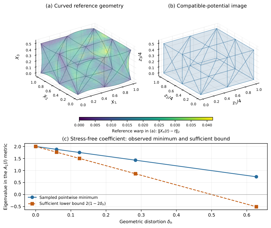
The complete $90$ -case comparison uses physical maps $y_{h}(X)=FX$ with deformation gradients $F=I_{3}$ , $I_{3}+(1/4)E_{12}$ and $D+(1/8)E_{12}$ , bulk values $0,10,1000$ , and either the face clamp or a fixed vertex at $t=(0,0,0)$ . There are $88$ positive compatible references. The two failures occur at $\alpha=7/8$ , zero bulk, and the stretched state with $z_{h}=Z_{*}\overline{X}_{h}$ , outside the certified family of Proposition 21. Their minimum eigenvalues are $-0.0526$ and $-0.0533$ . The observed bulk values $10,1000$ restore positivity through the volume outer term; the defect-corrected constant references remain positive in these observations.

For matrix comparisons define $d(A;B)=\|A-B\|_{F}/\max\{1,\|B\|_{F}\}$ . An additional $18$ -case interior-curvature control gives matching potential traces and compatible/corrected operators agreeing to $1.31\times 10^{-15}$ in $d$ , with the corrected reference as $B$ . Curved boundary traces can give different gauges: the strongest case differs by $0.0775$ , normalized by the compatible gauge. These observations test the trace equivalence and its restrictions. The complete parameter and arithmetic records remain in Appendix F.

9.4.3 A nonuniform loaded-state restriction

A different $48$ -cell family uses the global quadratic reference map

X_{h}(t)=t+\alpha\bigl(t_{2}(1-t_{2}),t_{3}(1-t_{3}),t_{1}(1-t_{1})\bigr)^{T},\qquad\alpha\in\{0,1/4,1/2\}.

The two physical deformations are specified in construction coordinates by $y_{h}(X_{h}(t))=X_{h}(t)$ and $y_{h}(X_{h}(t))=DX_{h}(t)+\tfrac{1}{4}(t_{2}-1/2)^{2}e_{1}$ , with the same $D$ as above. The potential is $4\overline{X}_{h}$ at rest and $Z_{*}\overline{X}_{h}$ in the latter state, where $Z_{*}=\operatorname{diag}(191/4,191/4,0)$ . With $c_{1}=c_{2}=1$ , bulk values $0,10,1000$ , and either the full boundary or the face $t_{1}=0$ constrained, this gives $36$ complete operators. Reference and normalized-current gradient bounds certify their orientation and injectivity. All pressure-geometric contributions are retained.

For $\alpha=1/2$ with one face constrained and the nonuniform current state, the compatible reference’s smallest eigenvalue is $-0.0099687$ at zero bulk, while the defect-corrected constant reference has minimum $0.0093759$ . Both are positive at bulk $10$ . At bulk $1000$ , their minima are $-1.145760$ and $-0.800219$ . For the Euclidean-unit minimum eigenvector of the compatible reference, its isochoric-plus-gauge term contributes $1.174943$ , the positive cell-volume outer product $0.0048728$ , and the pressure-geometric term $-2.325576$ . The sum gives the observed negative eigenvalue, with eigenpair residual $7.99\times 10^{-13}$ . Deleting the geometric term would change the energy Hessian. This example identifies the extra pressure-dependent control needed to extend the stress-free theorem to a loaded family.

A separate same-trace potential perturbation leaves its exactly assembled gauge unchanged to the reported arithmetic scale but changes its four-point approximation. The complete record in Appendix F distinguishes boundary equivalence from cellwise exactness after an arbitrary potential change.

The supporting complete-pressure and near-kernel arithmetic checks retain their separate matrix and component scales. They do not turn a local compatibility identity into a uniform floating-point guarantee. See Appendix F.

10 Discussion and conclusions

MORTIS gives a discrete design theory for cofactor reference forms: the exact kernel identifies the available potentials, the coefficient loss quantifies their attainable material margins, and boundary compensation preserves the complete tangent. The tensor, anisotropic, serendipity and Tet10 classifications depend on the actual variation and potential spaces. Degree counting alone misses the one-high-axis exception and the mixed serendipity modes.

The optimized margin tests every matrix increment at the prescribed quadrature points. Attainment concerns the finite evaluation image; ideal-margin rigidity additionally requires the stated candidate-space and gradient-sampling assumptions. Fixed-candidate enrichment can lower the best certificate by linear order in curvature amplitude, uniformly in cell size. At the largest reported amplitude, the explicit potential loses $12.7094\%$ of its material margin, while every compatible candidate must lose at least $1.20153\%$ . The numerical optimum remains uncomputed. The separate constant-coefficient trade-off is sharp in its specified basis, norm and pointwise positivity class.

A material certificate, a physical coercivity estimate and a complete operator spectrum measure different properties. On the smooth tensor example, pressure refinement changes a selected-direction Rayleigh value while the material margin is unchanged. A Gauss-three material-metric difference also coexists with exact gauge integration. The norm-transfer lemma identifies the additional geometry and quadrature assumptions required for a physical bound. An essential constraint removing constants on one mesh does not alone supply a uniform Poincaré constant.

Compatible and defect-corrected potentials give the same exact assembled gauge when their full potential traces agree. The prescribed-trace repair changes a local representation of that operator; its finite-dimensional solvability does not imply a uniform repair bound or economical computation. With a full displacement clamp, the compatible reference equals the complete tangent. The resulting one-column exact-preconditioning observation is a consequence of this equality. The partial-boundary MINRES comparisons show no consistent advantage for the gauge alone. A useful approximation to the signed boundary Schur action would require separate cost and residual analysis.

The uniform quadratic-tensor theorem and the finite-shear certificates retain their complete material, geometry, quadrature and boundary hypotheses. Their recovered pressures vanish, so arbitrary nonnegative bulk moduli add nonnegative outer terms. The loaded example has a larger negative pressure-geometric contribution than its positive material-plus-gauge and volume-outer contributions. Omitting that term would change the equation. The exact boundary representation survives; reference positivity at nonzero pressure needs further control.

Rational and interval certificates prove the specified parameter ranges; sampled eigenvalues retain their numerical status. Near-kernel cofactor components can have small absolute error and large relative action error. Complete-action accuracy therefore depends on the signed composition and pressure terms [28, 29]. These restrictions leave the core distinction explicit: compatibility selects a representation, material margins certify local positivity, and the proved coercivity regimes establish when that choice yields a complete positive reference.

Appendix A Exact Tet10 gauge structure

This appendix gives the complete coordinate derivations for the sharp tetrahedral instance. They describe a local cubature component before displacement boundary elimination; global cancellation and pointwise material margins have their separately stated meanings.

Let

\widehat{T}=\{\xi\in\mathbb{R}^{3}:\xi_{i}\geq 0,\ \xi_{1}+\xi_{2}+\xi_{3}\leq 1\},\qquad\lambda_{0}=1-\xi_{1}-\xi_{2}-\xi_{3},\quad\lambda_{i}=\xi_{i}\ (i=1,2,3).

Write $\mathbb{P}_{r}(\widehat{T})$ for scalar polynomials of total degree at most $r$ . Tet10 maps and variations belong to $[\mathbb{P}_{2}(\widehat{T})]^{3}$ . Their quadratic Lagrange functions are $N_{i}=\lambda_{i}(2\lambda_{i}-1)$ and $N_{ij}=4\lambda_{i}\lambda_{j}$ . The tetrahedral rule $Q_{4}$ has weight $1/24$ at each permutation of

(\alpha_{4},\beta_{4},\beta_{4},\beta_{4}),\qquad\alpha_{4}=\frac{5+3\sqrt{5}}{20},\qquad\beta_{4}=\frac{5-\sqrt{5}}{20}.

It is exact through total degree two [24]. This notation is distinct from tensor polynomial spaces and tensor Gauss point counts.

For the affine parent Jacobian $J_{y}=D_{\xi}y_{h}$ , let $J_{y,a}$ be its four vertex values and $\overline{J}_{y}=\frac{1}{4}\sum_{a}J_{y,a}$ . The centered determinant identity is

Q_{4}[\det J_{y}]-\int_{\widehat{T}}\det J_{y}=c_{4}\sum_{a=0}^{3}\det(J_{y,a}-\overline{J}_{y}),\qquad c_{4}=\frac{3\sqrt{5}-5}{1800}.

(59)

The same identity is used in RUPA [22]. Here is a short derivation. Put $B_{a}=J_{y,a}-\overline{J}_{y}$ , so $\sum_{a}B_{a}=0$ . All determinant terms containing the mean have spatial degree at most two and integrate exactly. If $e_{3},e_{21},e_{111}$ are the cubic moment errors for $\lambda_{i}^{3}$ , $\lambda_{i}^{2}\lambda_{j}$ and $\lambda_{i}\lambda_{j}\lambda_{k}$ with distinct indices, quadratic exactness gives $e_{21}=-e_{3}/3$ and $e_{111}=e_{3}/3$ . The symmetric determinant expansion with $\sum_{a}B_{a}=0$ therefore gives $(e_{3}-3e_{21}+2e_{111})\sum_{a}\det B_{a}$ . Finally, $e_{3}=(\alpha_{4}^{3}+3\beta_{4}^{3})/24-1/120$ and $(8/3)e_{3}=c_{4}$ , proving (59). Polarization connects its Hessian to $\mathcal{T}_{e}(y_{h};u_{h},v_{h})$ in (7).

A.1 Current and reference geometry in the quadratic case

For fixed quadratic variations $u_{e},v_{e}$ and a constant physical coefficient $R\in\mathbb{M}$ , define

\mathcal{E}_{J}(y_{e};u_{e},v_{e})=\mathcal{T}_{e}(y_{e};u_{e},v_{e}),\qquad\mathcal{E}_{C}(X_{e},R;u_{e},v_{e})=\mathcal{T}_{e}(RX_{e};u_{e},v_{e}).

The pullbacks (8) and (9) identify these with the determinant- and constant-coefficient cofactor-curvature errors, respectively.

Theorem 22 (Current and reference geometry in the quadratic defect).

For quadratic maps and variations, both defining integrands have total degree at most three. The determinant error is linear in the current parent Jacobian and vanishes when the current map is parent-affine. The cofactor error is linear in the reference parent Jacobian and vanishes when the reference map is parent-affine. For parent-affine maps $\overline{y}_{e},\overline{X}_{e}$ and a scalar $s$ ,

\mathcal{E}_{J}(\overline{y}_{e}+s(y_{e}-\overline{y}_{e});u_{e},v_{e})=s\mathcal{E}_{J}(y_{e};u_{e},v_{e}),

\mathcal{E}_{C}(\overline{X}_{e}+s(X_{e}-\overline{X}_{e}),R;u_{e},v_{e})=s\mathcal{E}_{C}(X_{e},R;u_{e},v_{e}).

Proof.

Each parent gradient is affine, and the determinant polarization is trilinear in its three gradient arguments. The integrand consequently has degree at most three. A constant first gradient leaves a product of degree at most two, which $Q_{4}$ integrates exactly. Linearity in that gradient proves both scaling identities. ∎

The result is specific to quadratic variations and the stated rule. At higher order, an affine first argument need not make the remaining gradient product exact. A variable constitutive coefficient also keeps its variation in the original quadrature form; the cofactor dependence stated above concerns the fixed coefficient $R$ .

A.2 An opposite-edge determinant representation

For a quadratic vector map $y_{h}$ , let $y_{i}$ be its vertex values and $y_{ij}$ its edge-midpoint values. Define the midside deviations by $d_{ij}(y_{h})=y_{ij}-(y_{i}+y_{j})/2$ , and write $d_{ij}=d_{ij}(y_{h})$ . We use the edge order $(01,12,20,03,13,23)$ , with $d_{20}=d_{02}$ . More generally $d_{ji}=d_{ij}$ , since the deviations are independent of edge orientation. Let $d\in\mathbb{R}^{18}$ collect these six vectors. Define two three-by-three matrices by listing their columns:

D_{+}(d)=[d_{01}+d_{23},\,d_{12}+d_{03},\,d_{20}+d_{13}],\qquad D_{-}(d)=[d_{01}-d_{23},\,d_{12}-d_{03},\,d_{20}-d_{13}].

Let $\mathscr{V}(d)$ be the scalar determinant cubature defect in (59). Its Hessian in the Euclidean midside-deviation coordinates is denoted by $\mathscr{R}(d)\in\mathbb{R}^{18\times 18}$ .

Theorem 23 (Opposite-edge normal form).

For every quadratic map,

\mathscr{V}(d)=16c_{4}\bigl(\det D_{-}(d)-2\det D_{+}(d)\bigr).

Proof.

The affine part of $y_{h}$ drops out of (59). Write $g_{a}=\nabla_{\xi}\lambda_{a}$ , so $g_{0}=(-1,-1,-1)^{T}$ and $g_{1},g_{2},g_{3}$ are the Cartesian unit vectors. For the quadratic part $4\sum_{i<j}\lambda_{i}\lambda_{j}d_{ij}$ , the centered vertex Jacobian is

\delta J_{y,a}=4\sum_{j\neq a}d_{aj}\otimes g_{j}-\sum_{i<j}d_{ij}\otimes(g_{i}+g_{j}).

Put $P=D_{+}(d)$ and $M=D_{-}(d)$ . Substitution gives $\delta J_{y,a}=PA_{a}+MB_{a}$ , with the following constant matrices:

\begin{array}[]{c|cc}a&A_{a}&B_{a}\\ \hline\cr 0&\begin{bmatrix}2&0&0\\ 0&0&2\\ 0&2&0\end{bmatrix}&\begin{bmatrix}2&1&1\\ -1&-1&-2\\ 1&2&1\end{bmatrix}\\[5.0pt] 1&\begin{bmatrix}-2&-2&-2\\ 0&2&0\\ 0&0&2\end{bmatrix}&\begin{bmatrix}-2&-1&-1\\ -1&1&0\\ 1&0&-1\end{bmatrix}\\[5.0pt] 2&\begin{bmatrix}0&0&2\\ 2&0&0\\ -2&-2&-2\end{bmatrix}&\begin{bmatrix}0&1&-1\\ 1&-1&0\\ -1&-2&-1\end{bmatrix}\\[5.0pt] 3&\begin{bmatrix}0&2&0\\ -2&-2&-2\\ 2&0&0\end{bmatrix}&\begin{bmatrix}0&-1&1\\ 1&1&2\\ -1&0&1\end{bmatrix}.\end{array}

They satisfy

\sum_{a}\det A_{a}=-32,\quad\sum_{a}\det B_{a}=16,\quad\sum_{a}B_{a}(\operatorname{cof}A_{a})^{T}=0,\quad\sum_{a}A_{a}(\operatorname{cof}B_{a})^{T}=0.

Use $\det(U+V)=\det U+\det V+\operatorname{cof}U{:}V+\operatorname{cof}V{:}U$ . Cofactor multiplicativity makes the two mixed sums vanish by the displayed matrix identities. Therefore $\sum_{a}\det(\delta J_{y,a})=-32\det P+16\det M$ . Multiplication by $c_{4}$ proves the result. ∎

A.3 Extension to symmetric quadratic-exact rules

A cubature rule $Q$ on $\widehat{T}$ is fully symmetric if it is unchanged by every permutation of the four barycentric coordinates. It is quadratic-exact if it integrates every scalar polynomial of total degree at most two exactly. Symmetric moment reduction is classical; the invariant-polynomial basis for tetrahedral rules is treated systematically by Wang and Papanicolopulos [30]. We use its degree-three consequence to identify the rule dependence of the preceding operator.

For such a rule, define its cubic moment defect and coefficient by

m_{3}(Q)=Q[\lambda_{0}^{3}]-\frac{1}{120},\qquad c_{Q}=\frac{8}{3}m_{3}(Q).

The integral of $\lambda_{0}^{3}$ on the unit parent tetrahedron is $1/120$ .

Proposition 24 (One rule-dependent cubic coefficient).

Let $J(\lambda)=\sum_{a=0}^{3}\lambda_{a}J_{a}$ be any affine three-by-three matrix field, and put $\bar{J}=\frac{1}{4}\sum_{a}J_{a}$ . Every fully symmetric quadratic-exact rule satisfies

Q[\det J]-\int_{\widehat{T}}\det J=c_{Q}\sum_{a=0}^{3}\det(J_{a}-\bar{J}).

Consequently the Tet10 scalar defect has the same opposite-edge normal form as in Theorem 23, with $c_{4}$ replaced by $c_{Q}$ . Moreover, $c_{Q}=0$ if and only if $Q$ is exact through degree three.

Proof.

Let $\mathcal{L}_{Q}$ denote cubature minus exact integration. It is invariant under the permutation group and annihilates quadratic polynomials. Symmetrizing a polynomial therefore leaves its $\mathcal{L}_{Q}$ value unchanged. Modulo polynomials of degree at most two, the symmetric cubic space is one-dimensional: the elementary symmetric polynomials have degrees one, two, three, and four, and the degree-one polynomial $\sum_{a}\lambda_{a}$ is the constant one on $\widehat{T}$ .

For a cubic polynomial $f$ on the barycentric hyperplane $\sum_{a}\lambda_{a}=1$ , let $f_{3}$ be the homogeneous degree-three part of its Taylor expansion about the barycenter. Let $v_{a}$ be the four barycentric vertex vectors and $\bar{v}=(1/4,1/4,1/4,1/4)$ . The functional $\mathcal{N}(f)=\sum_{a}f_{3}(v_{a}-\bar{v})$ is also invariant and annihilates quadratics. For $f=\lambda_{0}^{3}$ , it equals $(3/4)^{3}+3(-1/4)^{3}=3/8$ , so it is nonzero. The one-dimensional quotient gives $\mathcal{L}_{Q}=c_{Q}\mathcal{N}$ on cubics. For $f=\det J$ , its homogeneous cubic part at $v_{a}-\bar{v}$ is $\det(J_{a}-\bar{J})$ , proving the formula. The same quotient proves the final assertion. ∎

When $c_{Q}\neq 0$ , the local faithfulness and alignment results below, and the corresponding constant-gauge defect comparison, transfer to this rule. Norm formulas use $|c_{Q}|$ in place of $c_{4}$ ; a negative coefficient reverses the local signs. When $c_{Q}=0$ , these cubic defects vanish for every geometry, so an alignment restriction is unnecessary for these components. This concerns the constant-coefficient minor terms. The complete material energy and its rational pullbacks have additional quadrature dependence. Changing $Q$ in the complete energy defines a different discrete equation.

A.4 Norm, rank, and sign of the four-point defect

For a three-by-three matrix $A$ , let $\mathsf{D}(A)$ denote the nine-by-nine matrix of $D^{2}\det(A)$ in a Frobenius-orthonormal entry basis. Vectorizing $D_{+}(d)/\sqrt{2}$ and $D_{-}(d)/\sqrt{2}$ defines an orthogonal change of the eighteen coordinates. Denote that change by $T$ .

Corollary 25 (Faithfulness and an exact norm).

The Hessian has the orthogonal block representation

T\mathscr{R}(d)T^{T}=\operatorname{diag}\bigl(-64c_{4}\mathsf{D}(D_{+}(d)),32c_{4}\mathsf{D}(D_{-}(d))\bigr).

Consequently

\|\mathscr{R}(d)\|_{F}^{2}=4096c_{4}^{2}\bigl(4\|D_{+}(d)\|_{F}^{2}+\|D_{-}(d)\|_{F}^{2}\bigr).

(60)

In particular,

64\sqrt{2}\,c_{4}\|d\|_{2}\leq\|\mathscr{R}(d)\|_{F}\leq 128\sqrt{2}\,c_{4}\|d\|_{2}.

The map $d\mapsto\mathscr{R}(d)$ is injective. Its singular values, for these domain and matrix norms, are $64\sqrt{2}c_{4}$ and $128\sqrt{2}c_{4}$ , each with multiplicity nine.

Proof.

Differentiate Theorem 23 in the orthogonal coordinates. Each opposite-edge sum or difference is $\sqrt{2}$ times its new coordinate; the two derivative factors give the displayed blocks. In an entry basis, every entry of $A$ occurs in four signed entries of $\mathsf{D}(A)$ , and different entries have disjoint supports. Thus $\|\mathsf{D}(A)\|_{F}^{2}=4\|A\|_{F}^{2}$ , proving (60). The opposite-edge identity $\|D_{+}(d)\|_{F}^{2}+\|D_{-}(d)\|_{F}^{2}=2\|d\|_{2}^{2}$ gives the bounds. The sum and difference subspaces each have dimension nine; the norm identity gives the two singular values on them. ∎

These norms concern the stated quotient coordinates. A physical energy norm requires the element gradient metric. The two-to-one singular-value ratio concerns the geometry-to-matrix map. The action of an individual matrix on directions near its kernel can still be sensitive. Relative action errors then require the magnitude of that action as well as the matrix norm [28].

The determinant-Hessian calculation uses standard constitutive spectral algebra [18, 19]. The normal form identifies its precise occurrence in the Tet10 cubature operator.

For a real symmetric matrix $S$ , let $\operatorname{In}(S)=(n_{+}(S),n_{-}(S),n_{0}(S))$ count its positive, negative and zero eigenvalues, including multiplicity.

Corollary 26 (Local rank and sign).

The inertia of $\mathscr{R}(d)$ is the sum of the inertias of $-\mathsf{D}(D_{+}(d))$ and $\mathsf{D}(D_{-}(d))$ . For any $A\in\mathbb{M}$ , the determinant Hessian has inertia

\begin{array}[]{c|c}\text{condition on }A&\operatorname{In}(\mathsf{D}(A))\\ \hline\cr\operatorname{rank}A=0&(0,0,9)\\ \operatorname{rank}A=1&(2,2,5)\\ \operatorname{rank}A=2&(3,3,3)\\ \det A>0&(4,5,0)\\ \det A<0&(5,4,0).\end{array}

Every nonzero local cubic defect Hessian is indefinite.

Proof.

The first assertion follows from the orthogonal block representation and $c_{4}>0$ . If $A$ is invertible, write an increment as $H=AX$ . Then $D^{2}\det(A)[H,H]=\det A((\operatorname{tr}X)^{2}-\operatorname{tr}(X^{2}))$ . The trace direction and three skew directions are positive, and the five symmetric trace-free directions are negative, when $\det A>0$ . The signs reverse when $\det A<0$ . Invertible changes of left and right coordinates reduce a rank-two matrix to $\operatorname{diag}(1,1,0)$ and a rank-one matrix to $\operatorname{diag}(1,0,0)$ , up to a nonzero scalar factor. Direct expansion gives three positive and three negative directions in the first case and two of each in the second; the remaining directions vanish. A scalar sign cannot change these balanced counts. Rank zero gives the zero matrix. If $d\neq 0$ , at least one of $D_{+}(d),D_{-}(d)$ is nonzero. Its determinant-Hessian block has both signs. ∎

Local indefiniteness supplies no universal sign conclusion for a constrained assembled correction; assembly can remove local directions.

A.5 Exactness of a geometry-aligned translation

Let $d_{e}(X)$ denote the six reference-map midside deviations on one element, and let $\mathcal{C}_{X}=\operatorname{span}\{d_{ij}(X):i<j\}\subset\mathbb{R}^{3}$ . For a constant physical cofactor coefficient $Z$ , write $\mathsf{E}_{X}(Z)$ for the eighteen-coordinate matrix of $\mathcal{T}_{e}(ZX_{e};\cdot,\cdot)$ , with the tetrahedral four-point error functional. The potential pullback is $ZX_{e}$ , whose parent gradient is $ZJ_{X,e}$ . Here $Zd_{e}(X)$ means that $Z$ acts on each of the six vectors.

Proposition 27 (Necessary and sufficient alignment).

The following conditions are equivalent:

\mathsf{E}_{X}(Z)=0,\qquad Zd_{e}(X)=0,\qquad Z\mathcal{C}_{X}=\{0\},\qquad ZX_{h}\text{ is parent-affine}.

Proof.

The common polarized functional gives $\mathsf{E}_{X}(Z)=\mathscr{R}(Zd_{e}(X))$ . Corollary 25 makes its vanishing equivalent to $Zd_{e}(X)=0$ . The span condition is the same statement. A quadratic map is affine precisely when all its midside deviations vanish, giving the last equivalence. ∎

Thus the determinant tangent is exact under the four-point rule for every local pair of displacement variations precisely when its current quadratic map is affine. Exact scalar volume at a curved map is a weaker property. Let $W_{\rm iso}$ be any twice-differentiable isochoric density. A full three-dimensional space $\mathcal{C}_{X}$ also obstructs a positive exactly aligned gauge at every deformation: alignment forces $Z=0$ , while scale invariance gives $D^{2}W_{\rm iso}(F)[F,F]=0$ .

Appendix B First- and second-minor material calculus

The identities here close the constitutive derivation used by the reference forms. Fix $F\in\mathrm{GL}^{+}(3)$ and write $J=\det F$ , $C=\operatorname{cof}F$ , $I_{1}=F{:}F$ , $I_{2}=C{:}C$ . For increments $H,L$ , put $\theta_{H}=F^{-T}{:}H$ and define $\theta_{L}$ similarly. The form $Q_{F}$ , its rescaling $A_{1}$ and the coefficient $\pi_{1}$ were defined in (12)–(14).

B.1 The first-minor completed square

The form $Q_{F}$ is positive definite: if its sum of squares in (12) vanishes, $I_{1}>0$ forces $\theta_{H}=0$ , and its remaining square forces $H=0$ . Symmetry and bilinearity are immediate. To derive (15), differentiation of $\bar{I}_{1}=J^{-2/3}I_{1}$ gives

D\bar{I}_{1}(F)[H]=2J^{-2/3}\left(F{:}H-\frac{I_{1}}{3}\theta_{H}\right).

A second differentiation, using $D\theta_{H}(F)[L]=-\operatorname{tr}(F^{-1}LF^{-1}H)$ , yields

	$\displaystyle D^{2}\bar{I}_{1}(F)[H,L]={}$	$\displaystyle 2J^{-2/3}H{:}L-\frac{4}{3}J^{-2/3}\bigl(\theta_{L}F{:}H+\theta_{H}F{:}L\bigr)$
		$\displaystyle+\frac{4I_{1}}{9}J^{-2/3}\theta_{H}\theta_{L}+\frac{2I_{1}}{3}J^{-2/3}\operatorname{tr}(F^{-1}HF^{-1}L).$

Expanding $Q_{F}$ and substituting (1) rewrites this as $A_{1}(F)[H,L]-\pi_{1}(F)D^{2}J(F)[H,L]$ , as claimed. This is the first-minor Flory identity also used by the companion RUPA analysis [22]; its derivation is included here.

B.2 The cofactor chain rule

Write $K_{F}(H)=D\operatorname{cof}(F)[H]$ as in (3). The modified second invariant can be read as a first-invariant Flory function of the cofactor:

\bar{I}_{2}(F)=(\det C)^{-2/3}C{:}C,\qquad\det C=J^{2}.

(61)

This observation permits reuse of the completed square in (12), followed by an exact cofactor chain rule.

For $M,N\in\mathbb{R}^{3\times 3}$ , define

$\displaystyle\vartheta_{M}$	$\displaystyle=C^{-T}{:}M,$	(62)
$\displaystyle\vartheta_{N}$	$\displaystyle=C^{-T}{:}N,$	(63)
$\displaystyle Q_{C}(M,N)$	$\displaystyle=\left(M-\frac{2}{3}\vartheta_{M}C\right){:}\left(N-\frac{2}{3}\vartheta_{N}C\right)+\frac{I_{2}}{9}\vartheta_{M}\vartheta_{N}.$	(64)

The same sum-of-squares proof as for $Q_{F}$ shows that $Q_{C}$ is positive definite. Introduce

$\displaystyle A_{C}(F)[H,L]$	$\displaystyle=2J^{-4/3}Q_{C}(K_{F}(H),K_{F}(L)),$	(65)
$\displaystyle\pi_{C}(F)$	$\displaystyle=\frac{2I_{2}}{3J^{10/3}},$	(66)
$\displaystyle P_{C}(F)$	$\displaystyle=2J^{-4/3}\left(C-\frac{I_{2}}{3}C^{-T}\right).$	(67)

Theorem 28 (Completed second-invariant Hessian).

For every $F\in\mathrm{GL}^{+}(3)$ and $H,L\in\mathbb{R}^{3\times 3}$ ,

	$\displaystyle D^{2}\bar{I}_{2}(F)[H,L]={}$	$\displaystyle A_{C}(F)[H,L]-2\pi_{C}(F)DJ(F)[H]DJ(F)[L]$
		$\displaystyle-\pi_{C}(F)JD^{2}J(F)[H,L]+P_{C}(F){:}(H\times L).$		(68)

The form $A_{C}$ is positive definite on $\mathbb{R}^{3\times 3}$ .

Proof.

Define $\phi(C)=(\det C)^{-2/3}C{:}C$ . Applying the first-invariant identity (15) with $C$ as the matrix variable gives

D^{2}\phi(C)[M,N]=2J^{-4/3}Q_{C}(M,N)-\pi_{C}D^{2}\det(C)[M,N].

(69)

Its first derivative is

D\phi(C)[M]=P_{C}{:}M.

(70)

We next evaluate the determinant term after cofactor pullback. Since $\det(\operatorname{cof}F)=J^{2}$ , twice differentiating this composition yields

\displaystyle D^{2}\det(C)[K_{F}(H),K_{F}(L)]+D\det(C){:}(H\times L)=2DJ[H]DJ[L]+2JD^{2}J[H,L].

Here $D\det(C)=\operatorname{cof}C=JF$ , and (5) gives $D\det(C){:}(H\times L)=JD^{2}J[H,L]$ . Therefore

D^{2}\det(C)[K_{F}(H),K_{F}(L)]=2DJ[H]DJ[L]+JD^{2}J[H,L].

(71)

The second-order chain rule for $\bar{I}_{2}=\phi\circ\operatorname{cof}$ is

D^{2}\bar{I}_{2}[H,L]=D^{2}\phi(C)[K_{F}(H),K_{F}(L)]+D\phi(C){:}(H\times L).

Substitution of (69), (70), and (71) proves (68).

The form $Q_{C}$ is positive definite, $J^{-4/3}>0$ , and $K_{F}$ is invertible by Lemma 1. Their pullback $A_{C}$ is therefore positive definite. ∎

The second-invariant factor that will join the first-minor gauge is

B_{2}(F)=A_{C}(F)-2\pi_{C}(F)DJ(F)\otimes DJ(F).

(72)

It is obtained from the positive form $A_{C}$ by subtracting one scalar outer product, so its sign can depend on the deformation.

For fixed nonnegative coefficients $c_{1},c_{2}$ with $c_{1}+c_{2}>0$ , write $W_{\rm MR}$ for the cell density in (11). Define the two-minor gauge

G_{\rm MR}(F)=c_{1}A_{1}(F)+c_{2}B_{2}(F).

(73)

Define the combined determinant-curvature coefficient by

\Pi_{J}(F)=c_{1}\pi_{1}(F)+c_{2}\pi_{C}(F)J.

(74)

Combining (15) and Theorem 28 gives the full isochoric Hessian

	$\displaystyle D^{2}W_{\rm MR}(F)[H,L]={}$	$\displaystyle G_{\rm MR}(F)[H,L]-\Pi_{J}(F)D^{2}J(F)[H,L]$
		$\displaystyle+c_{2}P_{C}(F){:}(H\times L),$		(75)

The last two terms are respectively determinant and cofactor curvature.

On a rank-one increment $H=a\otimes n$ , both $D^{2}J(F)[H,H]$ and $H\times H=2\operatorname{cof}H$ vanish. Thus the complete rank-one isochoric value in (75) equals $G_{\rm MR}(F)[H,H]$ . Positivity of that chosen gauge is a sufficient rank-one ellipticity condition. The exact decomposition keeps both curvature channels available for the discrete compatibility and compensation analysis.

Appendix C Exact non-aligned reference geometry

These data specify the reference mesh in Proposition 20. The deformation, point metric $A_{1}(D)$ and full interval-congruence argument are given in Section 8; the integer coordinates below complete that specification.

Divide each axis of $[0,1]^{3}$ into two intervals. Split each of the eight cubes into the six tetrahedra whose vertex paths increment the three coordinate directions in each possible order. Use an orientation-preserving local vertex order and the six midside nodes of the quadratic element. The resulting parameter nodes form the quarter grid $t=(i,j,k)/4$ , $0\leq i,j,k\leq 4$ . The Cartesian vectors $e_{1},e_{2},e_{3}$ determine the coordinate directions; the current fields use the fixed matrix $D=\operatorname{diag}(2,2,1/4)$ and $E_{12}=e_{1}\otimes e_{2}$ defined with the shear family.

Set $X(t)=t$ at every boundary node, and set $X_{2}=t_{2}$ , $X_{3}=t_{3}$ at every node. For the interior nodes, define integers $n_{ijk}$ by Table 5 and set $X_{1}(i/4,j/4,k/4)=n_{ijk}/2^{55}$ . These rational coordinates specify the geometry independently of the sampling procedure that first produced it.

Table 5: Exact first-coordinate numerators for the non-aligned reference mesh. The common denominator is

2^{55}

$j$	$k$	$n_{1jk}$	$n_{2jk}$	$n_{3jk}$
1	1	9105314122432956	17060509236021852	28356459511241252
1	2	12049108527703530	17816379473272022	27203240556309152
1	3	7623885483807398	19502005720601204	26157924656613804
2	1	10316193290055142	16881392942710108	27515618967020928
2	2	8671466383741623	16989823806708642	24586724701378688
2	3	11123479124564504	19221453749166012	24175413339273560
3	1	11432525502845932	17898559407134226	29511977488033696
3	2	7213745460801190	18134896708814432	27423007014701600
3	3	9189194271142126	18086850943127236	27280126714252592

Appendix D Full-curvature compatible-potential mesh

This is the exact reference geometry for Proposition 21. Its complete finite-shear proof and the physical quadrature metric $A_{I,h}$ are in Section 8. The integer table and its normalization below specify the certificate inputs.

Partition each cube of the corner grid $\{0,1/2,1\}^{3}$ into the six Freudenthal tetrahedra given by the coordinate-order paths. The resulting quadratic mesh has $48$ cells and $125$ nodes, at $t=(i,j,k)/4$ with $i,j,k\in\{0,1,2,3,4\}$ . Let $a_{h}$ be the continuous parent-quadratic vector field whose nodal values are the integer vectors in Table 6; its values are zero when all three indices are even. The rational reference map is

X_{h}(t)=t+\frac{7}{3768}a_{h}(t).

Thus every reference corner is unchanged, and $\overline{X}_{h}(X_{h}(t))=t$ , where $\overline{X}_{h}$ is the continuous corner-linear potential field. The table uses the three-digit key $ijk$ for the node $(i,j,k)/4$ , with vector components $(a_{1},a_{2},a_{3})$ .

Let $v_{e,a}$ denote the parameter-cell corners. The matrix $1$ - and $\infty$ -norms are the maximum absolute column and row sums. The integer vertex derivatives satisfy

\max_{e,a}\left\lVert D_{t}a_{h}(v_{e,a})\right\rVert_{1}\,\left\lVert D_{t}a_{h}(v_{e,a})\right\rVert_{\infty}=221760.

The spectral norm is bounded by the square root of this product. Since $D_{t}a_{h}$ is affine on each cell, convexity of the spectral norm extends the vertex bound to the whole cell. Therefore

\left\lVert D_{t}X_{h}-I_{3}\right\rVert_{2}\leq\frac{7}{3768}\sqrt{221760}=\sqrt{\frac{18865}{24649}}<1.

The perturbation is globally Lipschitz on the convex parameter cube with this constant. The map is strongly monotone and hence injective; its Jacobian is invertible with positive determinant. Nonzero integer three-by-three minors of the six edge-deviation vectors verify full three-directional curvature on all cells.

The compatible-core verification package described in Section F.9 contains the node and connectivity arrays, integer minor witnesses, the rational Bernstein matrices, and all interval elimination records for Proposition 21. Coordinate enclosures include both this rational map and its retained binary64 realization. The proof concerns the stated exact-real family; it makes no assertion of uniformly accurate floating-point arithmetic as the bulk moduli tend to infinity.

Table 6: Integer nodal coefficients of

a_{h}

. All-even node indices have coefficient

(0,0,0)

and are omitted.

$ijk$	$a_{1}$	$a_{2}$	$a_{3}$	$ijk$	$a_{1}$	$a_{2}$	$a_{3}$	$ijk$	$a_{1}$	$a_{2}$	$a_{3}$
001	-5	15	7	132	-14	-9	7	314	9	-15	-11
003	5	-2	-5	133	-11	-2	7	320	6	16	-12
010	12	-10	-10	134	-6	-6	9	321	-7	12	8
011	2	-4	2	140	-7	-13	-4	322	-5	-2	7
012	-10	4	12	141	9	-5	9	323	-3	-11	-6
013	13	2	-4	142	4	1	0	324	5	15	14
014	8	9	-9	143	12	10	14	330	-2	13	10
021	-15	9	6	144	-1	-9	-12	331	-8	-14	-8
023	7	-10	10	201	-3	3	-1	332	-6	-10	-16
030	4	6	16	203	3	-7	-1	333	11	2	7
031	-3	-11	-3	210	6	-15	11	334	3	11	-5
032	-9	1	-4	211	-3	-16	-3	340	-2	9	2
033	0	-8	-8	212	-8	7	-16	341	15	1	11
034	8	-8	10	213	-11	11	1	342	0	12	8
041	9	-3	-8	214	-1	-9	-12	343	7	12	-6
043	14	-4	2	221	-9	15	4	344	16	-10	-6
100	-1	11	7	223	-13	16	-9	401	-14	14	8
101	13	4	1	230	-3	-5	10	403	8	-14	-3
102	-5	-2	13	231	-8	-12	-1	410	-12	-12	5
103	-9	4	-7	232	0	6	-9	411	11	-5	-14
104	8	-5	1	233	-9	-1	13	412	7	16	-2
110	-16	3	-8	234	2	6	-11	413	7	-14	12
111	12	0	9	241	-2	11	1	414	11	-2	-13
112	9	13	-12	243	11	-5	-15	421	-12	6	7
113	6	-4	-16	300	-4	-5	-8	423	-7	10	-2
114	2	2	15	301	8	-9	-7	430	-7	-13	10
120	7	-7	11	302	-4	-15	-2	431	16	-13	7
121	-13	-10	-6	303	-14	12	-3	432	13	-12	-10
122	-14	9	5	304	-6	-10	-10	433	11	-14	-11
123	-14	-10	2	310	2	15	-10	434	3	1	12
124	8	-5	11	311	9	-3	3	441	-8	-8	1
130	11	3	6	312	-10	-10	-16	443	-9	14	-14
131	-14	9	7	313	2	-13	-9

Appendix E Exact representatives with a prescribed potential trace

There is a finite-dimensional way to test whether a desired potential trace admits an exact representative. The construction uses ordinary orthogonal projection and least-squares algebra [28]; its constants depend on the selected coefficient and residual metrics. This is an auxiliary representation problem after the potential trace has been fixed. By Corollary 15, all its exact representatives give the same assembled added operator.

Give $\mathcal{Z}_{h}$ a specified Hilbert norm and let $\mathsf{D}:\mathcal{Z}_{h}\to\mathcal{Y}$ collect the cell defect forms $\mathcal{T}_{e}(z_{e};\cdot,\cdot)$ in fixed local bases, with a specified Hilbert norm on the residual space $\mathcal{Y}$ . Its kernel is $\mathcal{Z}_{h}^{0}$ . Let $\tau$ extract the full external potential trace, set $\mathcal{Z}_{b}=\ker\tau$ , and restrict $\mathsf{D}_{b}=\mathsf{D}|_{\mathcal{Z}_{b}}$ . Potential constants are not removed from these coordinates when their traces matter. Fix a lift $z_{0}$ of a desired trace $b=\tau z_{0}$ , and let $P_{b}$ be the $\mathcal{Y}$ -orthogonal projector onto $\operatorname{range}\mathsf{D}_{b}$ .

Proposition 29 (Trace obstruction and least-norm correction).

The vector $\eta_{b}=(I-P_{b})\mathsf{D}z_{0}$ is independent of the chosen lift of $b$ , and

\min_{\tau z=b}\|\mathsf{D}z\|_{\mathcal{Y}}=\|\eta_{b}\|_{\mathcal{Y}}.

An exactly compatible potential with trace $b$ exists precisely when $\eta_{b}=0$ . Among corrections attaining the minimum defect, the least-norm correction gives

z_{*}=z_{0}-\mathsf{D}_{b}^{\dagger}\mathsf{D}z_{0}.

(76)

Here the pseudoinverse uses the specified two Hilbert metrics. If $\eta_{b}=0$ and $\mathsf{D}_{b}$ has positive rank, let $\sigma_{b}$ and $\sigma_{\max}$ be its smallest positive and largest singular values. Then

\frac{\|\mathsf{D}z_{0}\|_{\mathcal{Y}}}{\sigma_{\max}}\leq\min_{\begin{subarray}{c}\tau z=b\\ \mathsf{D}z=0\end{subarray}}\|z-z_{0}\|_{\mathcal{Z}_{h}}=\|\mathsf{D}_{b}^{\dagger}\mathsf{D}z_{0}\|_{\mathcal{Z}_{h}}\leq\frac{\|\mathsf{D}z_{0}\|_{\mathcal{Y}}}{\sigma_{b}}.

Proof.

Every same-trace potential is $z_{0}+v$ , with $v\in\mathcal{Z}_{b}$ . The residual decomposes orthogonally as

\mathsf{D}(z_{0}+v)=\eta_{b}+(P_{b}\mathsf{D}z_{0}+\mathsf{D}_{b}v).

Changing the lift adds an element of $\operatorname{range}\mathsf{D}_{b}$ and leaves $\eta_{b}$ unchanged. The second summand can be set to zero by the pseudoinverse, proving the minimum defect and the exactness criterion. The singular-value decomposition gives the unique minimum-norm correction and the two bounds. When $\mathsf{D}_{b}$ has rank zero, the decomposition and (76) still apply; no positive singular-value denominator is used. ∎

Under the common-material-sum hypotheses of Section 4, take the ideal target $z_{0}=2c\iota$ . Suppose $z_{0}\in\mathcal{Z}_{h}$ and $\eta_{b}=0$ , and put $\delta z=\mathsf{D}_{b}^{\dagger}\mathsf{D}z_{0}$ . The exact margin formula in Section 4 gives

\gamma_{h}(z_{*})=c-\max_{e,q}\nu\!\left(-\nabla_{X}\delta z(X_{e}(\xi_{eq}))\right).

The minus sign is necessary because the loss function $\nu$ need not be symmetric. Define

L_{b}=\sup_{\begin{subarray}{c}v\in\mathcal{Z}_{b}\\ \|v\|_{\mathcal{Z}_{h}}=1\end{subarray}}\max_{e,q}\nu\!\left(-\nabla_{X}v(X_{e}(\xi_{eq}))\right),

with $L_{b}=0$ if $\mathcal{Z}_{b}=\{0\}$ . Positive homogeneity and the pseudoinverse estimate give

\gamma_{h}(z_{*})\geq c-\frac{L_{b}}{\sigma_{b}}\|\mathsf{D}z_{0}\|_{\mathcal{Y}}

when $\sigma_{b}$ exists. Exact kernel dimension and finite-dimensional solvability do not bound $L_{b}/\sigma_{b}$ uniformly in mesh size or order. Such a conclusion requires control of the stated physical gradients and metrics.

Every exact representative of the same trace gives the same assembled gauge Hessian. Thus the repair constructs a locally exact representation of the defect-corrected target operator. A solver benefit or a uniform repair cost requires additional numerical analysis.

Appendix F Supporting observations and arithmetic controls

These records supply the complete parameters, operator comparisons and arithmetic qualifications behind Section 9. They retain the original equations, numerical outcomes and adverse choices. Computed eigenvalues remain distinct from the rational and interval sign certificates.

F.1 Normalization of high-precision bilinear comparisons

For the $70$ -digit checks of the aligned and non-aligned families, let $A_{e}^{64}\in\mathbb{R}^{30\times 30}$ be the computed complete cell Hessian and let $u_{e},v_{e}\in\mathbb{R}^{30}$ be the nodal variation vectors. Let $b_{64}$ be their bilinear value evaluated in binary64 and $b_{70}$ the independently differentiated scalar energy value at $70$ decimal digits. The reported discrepancy is

e_{\rm bil}=\frac{|b_{64}-b_{70}|}{s_{64}},\qquad s_{64}=\operatorname{fl}_{64}\bigl(\|A_{e}^{64}\|_{F}\,\|u_{e}\|_{2}\,\|v_{e}\|_{2}\bigr).

(77)

Here $\operatorname{fl}_{64}$ denotes the binary64 evaluation of the norms and their product. Stored nodal values are promoted exactly, and the independent differentiation uses the ideal four-point rule. The $80$ -digit comparisons below use their separately stated reference-bilinear normalization.

F.2 Normal form and a fixed geometry-aligned coefficient

The opposite-edge normal form was checked independently in integer arithmetic. All $18^{3}=5{,}832$ entries of the polarized tensor agreed exactly, as did $32$ integer cubic examples. The exact Gram matrix of the geometry-to-Hessian map gives squared singular values $8192c_{4}^{2}$ and $32768c_{4}^{2}$ , each nine times, in the coordinates of Corollary 25. The four printed vertex-matrix identities were also checked as integer equalities.

Three positive-weight rational cubature rules checked the rule dependence in Proposition 24. A centroid/vertex rule with five points gives $c_{Q}=1/180$ ; a centroid/edge-midpoint rule with seven points gives $c_{Q}=-1/360$ ; an eleven-point combination gives $c_{Q}=0$ . All quadratic moments were exact. The last rule also integrated every cubic moment exactly. Twenty-four independently generated affine matrix fields per rule satisfied the determinant identity with zero rational discrepancy. These rules test positive, negative, and zero defect coefficients.

The aligned coefficient $\operatorname{diag}(45,45,0)$ had negative gauge curvature near the endpoints of the shear interval $[-1/4,1/4]$ . Its five sampled minimum eigenvalues in the $A_{1}(D)$ metric were approximately $-0.9692,-0.0833,0.4844,-0.0833,-0.9692$ . Allowing the diagonal coefficient to vary in joint selection over the same interval gave $Z_{*}=\operatorname{diag}(191/4,191/4,0)$ after rationalization. The five observed minima became $0.2241,0.2890,0.3275,0.2890,0.2241$ . The rational Bernstein certificate in Proposition 19 establishes positivity between the sampled states. The failed coefficient and the successful certificate are both recorded.

F.3 Complete-pressure boundary reconstruction

The parameter cube $[0,1]^{3}$ was divided into $n^{3}$ cubes, each split by the six Freudenthal tetrahedra. For a real curvature amplitude $\beta$ , shared quadratic nodes were mapped to a reference geometry by nodal interpolation of

X(t)=t+\beta\prod_{i=1}^{3}t_{i}(1-t_{i})e_{3}.

The polynomial in this display prescribes nodal values; each isoparametric cell map is quadratic. Its first two components are affine, so its Jacobian determinant is affine on each cell. Positive vertex determinants establish whole-cell orientation for this family. The first two components are unchanged and the third is strictly increasing along vertical lines, giving global injectivity with the fixed cube boundary.

The current map was the quadratic field $y_{h}(X)=DX+\epsilon(X_{2}-1/2)^{2}e_{1}$ associated with Proposition 19. For $n=2$ , we used $\beta\in\{0,8\}$ , $\epsilon\in\{-1/4,0,1/4\}$ , and $\kappa\in\{10,1000\}$ , with either a full boundary constraint or a constraint on the face $t_{1}=0$ . This gives $24$ complete operator cases. Four additional cases used $n=4$ , $\beta=8$ , $\epsilon=1/4$ , both bulk moduli, and both constraints. The large cases tested the boundary representation and the solve obtained by eliminating interior coordinates; iterative comparisons were omitted.

The complete matrix $K_{h}$ and translated matrix $G_{h}$ were assembled independently. A third route integrated the cofactor second variation over oriented external facets to form $B_{\Gamma}$ . Every pressure contribution was retained, including the small pressure-geometric term generated by binary64 rounding in the nominally volume-preserving cases. Table 4 reports the results. The reconstruction column is $\|K_{h}-G_{h}+R_{\Gamma}^{T}B_{\Gamma}R_{\Gamma}\|_{F}/\|K_{h}\|_{F}$ . For a seeded right-hand side $b$ and computed solution $x$ , the solve column is the independently recomputed relative residual $\|K_{h}x-b\|_{2}/\|b\|_{2}$ .

For this elimination, partition the free displacement coordinates into interior coordinates $i$ and free boundary coordinates $\Gamma$ . The Schur complement of the positive reference is

S_{G}=G_{\Gamma\Gamma}-G_{\Gamma i}G_{ii}^{-1}G_{i\Gamma},\qquad S_{K}=S_{G}-B_{\Gamma}.

The reduced complete solve uses $S_{K}$ . Since $G_{ii}\succ 0$ , all negative directions of the complete matrix are represented by $S_{K}$ . When $S_{G}\succ 0$ , the trace pencil is the generalized eigenvalue problem $S_{K}x_{\Gamma}=\lambda S_{G}x_{\Gamma}$ ; its negative eigenvalues give the partially constrained counts in the table.

For the $n=2$ comparison, both preconditioners used exact global Cholesky reference actions. One was the translated gauge; the other spectrally clipped the pointwise material Hessian and retained the positive cell-volume outer product. The complete matrix in the MINRES iteration was identical. The iteration stopped on an independently evaluated relative residual of $10^{-9}$ or at $240$ columns; these are diagnostic stopping settings. With a full constraint, the translated gauge equals the complete matrix, so its one-column result follows from exact preconditioning. The clipping reference took $17$ columns. With one face constrained, the gauge required $185$ – $240$ columns and reached the residual setting in nine of twelve cases; clipping required $194$ – $240$ columns and reached it in eleven. Neither solver shows a consistent partial-boundary advantage from the gauge alone. The explicit boundary Schur solve retained the complete indefinite equation in all cases.

Eight further cases uniformly dilated the $n=2$ , $\beta=8$ , $\epsilon=1/4$ field to $J=1\pm 1/1024$ , using both bulk moduli and constraints. The cell pressures were approximately $\pm 0.009765625$ and $\pm 0.9765625$ . Boundary reconstruction remained below $2.75\times 10^{-17}$ , and all complete trace-solve residuals were below $1.11\times 10^{-12}$ . For the compressed $\kappa=1000$ case, the minimum generalized eigenvalue of the full pointwise density gauge was approximately $-0.4202$ , although the assembled translated reference remained numerically positive by Cholesky factorization. That density omits the separate positive cell-volume outer product. Its pointwise sign alone therefore does not decide the assembled sign. A uniform nonzero-pressure extension of Proposition 19 would need its own argument.

Independent $70$ -digit differentiation of the complete scalar condensed energy checked eight local bilinear actions, with maximum discrepancy $4.916\times 10^{-17}$ using the normalization in (77). It used the exact promoted binary64 nodal values and the ideal four-point rule; quadrature-node rounding is consequently a separate error source. The $36$ cases are manufactured operator states. A load-controlled nonlinear trajectory and production-scale solver performance remain unmeasured.

F.4 Aligned and unaligned curvature under two rules

A complete-operator alignment comparison used the same $n=2$ mesh and a scalar continuous quadratic field $\psi_{h}$ with zero boundary values. Its interior nodal values were seeded normal samples. For an axis $a\in\{1,3\}$ , let $\psi_{h,a}$ be this field divided by the largest absolute vertex value of $\partial_{a}\psi_{h}$ over all cells. The reference map was $X(t)=t+\theta\psi_{h,a}(t)e_{a}$ , with $\theta\in\{0,1/4,1/2,3/4,0.9\}$ . Its determinant is $1+\theta\partial_{a}\psi_{h,a}$ . The vertex-slope normalization and the affine derivative give whole-cell orientation; the observed minimum relative reference Jacobian was $0.10$ . Fixed boundary values and one-component monotonicity give global injectivity.

The current deformation was $y=DX$ . Its physical gradient is exactly the specified $D$ , so the condensed pressure coefficient vanishes and the complete positive pressure outer product remains. The two axes, five amplitudes, three bulk moduli $0,10,1000$ , and two rules gave $60$ full-Dirichlet operator observations on $81$ free coordinates. The second rule was the positive eleven-point cubic-exact rule above. Each rule defined its own complete energy.

With curvature in the first direction, the four-point relative difference $\|G_{h}-K_{h}\|_{F}/\|K_{h}\|_{F}$ reached $5.86\times 10^{-4}$ . The cubic-exact rule reduced this cofactor compensation to the arithmetic scale. With curvature in the third direction, the coefficient $Z_{*}$ is aligned and both rules have compensation at that scale. All $60$ complete matrices remained numerically positive, with smallest eigenvalues at least $1.3796$ in the given nodal coordinates. The comparison agrees with the rule/alignment classification; it does not demonstrate an instability of the four-point complete equation, since a nonzero separated defect can coexist with assembled coercivity.

F.5 Defect-corrected reference observations on the certified mesh

The non-aligned geometry in Appendix C supplies $18$ complete-operator observations. They use deformation parameters $\epsilon=-1/4,0,1/4$ , bulk moduli $\kappa=0,10,1000$ , and either the full boundary or the face $t_{1}=0$ constrained. The reference defect is assembled once. Each translated matrix then subtracts that same defect, and an independent oriented-facet integral supplies the exact boundary form.

The largest relative recomposition discrepancy $\|K_{h}-\widehat{G}_{h}+R_{\Gamma}^{T}B_{\Gamma}R_{\Gamma}\|_{F}/\|K_{h}\|_{F}$ is $4.041\times 10^{-17}$ . Every corrected reference is numerically positive, and all complete trace solves have independent relative residual below $5.380\times 10^{-13}$ . For the one-face constraint, the numerical negative counts of the complete matrix are $31$ , $25$ , and $20$ at the three bulk moduli, respectively, at every sampled deformation. The corrected reference and the complete matrix therefore have distinct sign roles.

The largest arithmetic cell pressure is $5.785\times 10^{-13}$ ; all resulting pressure-geometric terms were retained. Three independent $70$ -digit scalar-energy bilinear checks have maximum discrepancy $8.223\times 10^{-17}$ under the normalization in (77). The interval theorem concerns the exact parametric deformation family; these observations also expose the rounding in its binary64 nodal construction. No uniform floating-point guarantee as the bulk modulus tends to infinity is inferred.

F.6 Complete finite-state and boundary-equivalence observations

Let $a_{h}$ be the integer-nodal perturbation field of Appendix D. The reference maps $X_{h}^{\alpha}=t+(\alpha/471)a_{h}(t)$ use $\alpha\in\{0,1/8,1/4,1/2,7/8\}$ . Figure 4 displays the strongest curved reference and its corner-linear coefficient potential.

With $D=\operatorname{diag}(2,2,1/4)$ , the physical maps $y_{h}(X)=FX$ with $F=I_{3}$ , $I_{3}+(1/4)E_{12}$ , and $D+(1/8)E_{12}$ , the bulk values $0,10,1000$ , and two essential-constraint sets give $90$ complete operator observations. The compatible potential is $4\overline{X}_{h}$ for the first two states and $Z_{*}\overline{X}_{h}$ for the third. The face constraint fixes variations on $t_{1}=0$ ; the vertex constraint fixes all three components at $t=(0,0,0)$ . All four nonzero-amplitude meshes have exactly certified three-directional curvature on every cell. For a computed matrix $A$ and a specified reference matrix $B$ , define the normalized difference $d(A;B)=\|A-B\|_{F}/\max\{1,\|B\|_{F}\}$ . The volume and oriented-face gauge matrices agree to $6.66\times 10^{-15}$ with the volume gauge as reference. The constant-gauge four-point defect reaches $0.0220$ with its exactly integrated gauge as reference. Three independent determinant-moment/face-minor checks agree exactly in rational arithmetic, including cancellation on interior faces. Six $80$ -digit differentiations of the complete material energy agree with the implemented bilinear forms to $1.61\times 10^{-14}$ after dividing the absolute difference by $\max\{1,|b_{\rm ref}|\}$ , where $b_{\rm ref}$ is the high-precision reference bilinear value.

The $90$ rows contain $88$ positive compatible references. The two failures occur at the strongest curved geometry, zero bulk modulus, and the more strongly stretched state $D+(1/8)E_{12}$ with potential $z_{h}=Z_{*}\overline{X}_{h}$ from Proposition 19. Their minimum eigenvalues are approximately $-0.0526$ and $-0.0533$ for the face and vertex constraints. The observed bulk values $10$ and $1000$ restore positivity through the additional volumetric outer term. The defect-corrected constant-gauge references remain positive in these observations. Exact gauge quadrature alone therefore does not imply an admitted positive reference at every material state.

An additional $18$ -row control curves only interior nodes. The two potential traces then agree, and the compatible and defect-corrected constant-gauge operators agree to $1.31\times 10^{-15}$ in $d$ , with the corrected reference as $B$ , as required by Corollary 15. With curved boundary traces they can differ; the strongest reference gives a normalized difference of $0.0775$ between the two gauge matrices, with the compatible gauge as reference. These findings identify a quadrature-compatible local construction and its coercivity regime, without claiming general nonlinear-solver speedup.

F.7 A trace-preserving potential change

Use the nonuniform family of Section 9.4.3 and the normalized matrix difference $d$ defined above. A separate potential comparison changes only one interior nodal value while preserving its entire boundary trace. Its exactly integrated assembled gauge changes by $4.248\times 10^{-16}$ in the normalization $d$ defined above; the four-point matrix changes by $0.0037862$ . Boundary equivalence therefore does not imply cellwise quadrature exactness after an arbitrary quadratic change of potential. This comparison clarifies the distinct assumptions on the potential trace and its cellwise polynomial space.

F.8 Supporting complete-pressure and arithmetic checks

The material identities were independently checked through direct differentiation of the scalar Mooney–Rivlin energy and through the cofactor chain rule in Appendix B. The continuous-family certificates use exact rational Bernstein coefficients and outward-enclosed matrix inequalities. Ordinary computed eigenvalues remain separate from those sign proofs.

A physical-state reconstruction with $176{,}982$ displacement coordinates and $34{,}295$ Tet10 cells illustrates the complete-pressure distinction. Of these cells, $26{,}613$ use condensed $P_{0}$ pressure and $7{,}682$ use quadrature-local volumetric penalties. Both compared matrices retain the latter cells’ contributions. The partial Hessian in this comparison omits the condensed pressure contributions $Q_{P0}+P_{P0}$ in (18)–(19). On that state it has $22$ negative eigenvalues reported by the sparse factorization, whereas the full reduced-energy Hessian has zero. The gauges and complete tangent were reconstructed from the same state, and the scope-difference identity closes to $2.149\times 10^{-16}$ relatively. These cuDSS counts are numerical factorization observations, without perturbation certification.

A small component also requires its own accuracy interpretation. For the constant-coefficient cofactor-defect component of that physical state, the matrix Frobenius norm is $5.7130\times 10^{-8}$ . Direct and parent-coordinate matrices differ in Frobenius norm by $1.9532\times 10^{-16}$ absolutely, or $3.4189\times 10^{-9}$ relative to that component. Restricted affine fields increase the relative action difference to $1.69\times 10^{-7}$ . This is near-kernel forward sensitivity, consistent with standard backward-versus-forward error analysis [28, 29]. A componentwise relative ratio is not the error of the complete tangent action. The observations limit claims of uniformly accurate independent application of a tiny correction. The exact compatibility and compensation identities themselves are unaffected.

F.9 Verification files for the finite-family certificates

The authors retain the proof objects and verification scripts for these finite families, available upon reasonable request and planned for public release in a subsequent version. The file aligned-shear.json gives the exact Bernstein matrices and rational pivots for the $1/5$ margin in Proposition 19. The nonaligned-core package contains the exact geometry, the $23/100$ material certificate, and the interval matrix endpoints and binary64 triangular transform used in the congruence proof. Its driver verify_core_certificate.py checks the geometry, material inequality and matrix enclosure.

The compatible-core package contains the integer geometry definition, rational material coefficients, all $8640$ retained pivot intervals, and the distortion witness. Its driver verify.py reconstructs the interval certificate. Each package has a README with extraction and execution instructions. These files specify the particular computational proofs reported above; the mathematical matrices and reconstruction formulas are also defined in Section 8 and Appendices C and D. The certificate programs use Python, NumPy, SciPy and mpmath, independently of the simulation framework.

CRediT author statement

Yanlin Liu originated the central theoretical ideas and mathematical formulations and led the theoretical development.

Yanlin Liu: Conceptualization (central theoretical ideas); Methodology (mathematical formulation and method development); Formal analysis (theoretical analysis and derivations); Software (research-specific development, framework extensions and performance optimization); Investigation; Validation; Writing—original draft; Writing—review and editing.

Kaixiang Yao: Conceptualization (application motivation for reducing warm execution time in repeated robotics simulations); Writing—review and editing.

Chao Huang: Software (development of the foundational simulation framework); Conceptualization (introduction of the underlying numerical problem and the near-incompressibility regime).

Yao Shen: Supervision; Resources (provision of computational resources); Conceptualization (broad problem introduction and research context).

Data and code availability

Interval certificates, exact verification data, constitutive verification scripts, and controlled inputs are available from the authors upon reasonable request. A public reproducibility repository is planned for a subsequent version. The private simulation platform and its production solvers are outside the planned release.

Declaration of generative AI use

OpenAI Codex was used to assist with experimental coding, preliminary mathematical review, and preliminary drafting. Anthropic Claude was used for draft reviewing and editing. Yanlin Liu provided the central theoretical ideas and initial mathematical formulations. Responsibility for the claims, citations, computational results, and final manuscript rests with the named authors.

References

[1] J. M. Ball (1976) Convexity conditions and existence theorems in nonlinear elasticity. Archive for Rational Mechanics and Analysis 63 (4), pp. 337–403. External Links: Document Cited by: §1, §2.1, §2.4.
[2] J. Schröder, P. Wriggers, and D. Balzani (2011) A new mixed finite element based on different approximations of the minors of deformation tensors. Computer Methods in Applied Mechanics and Engineering 200 (49–52), pp. 3583–3600. External Links: Document Cited by: §1, §2.1.
[3] J. Bonet, A. J. Gil, and R. Ortigosa (2015) A computational framework for polyconvex large strain elasticity. Computer Methods in Applied Mechanics and Engineering 283, pp. 1061–1094. External Links: Document Cited by: §1, §2.1.
[4] D. G. B. Edelen and D. C. Lagoudas (1986) Null Lagrangians, admissible tractions, and finite element methods. International Journal of Solids and Structures 22 (6), pp. 659–672. External Links: Document Cited by: §1, §4, §7.
[5] P. J. Olver and J. Sivaloganathan (1988) The structure of null Lagrangians. Nonlinearity 1 (2), pp. 389–398. External Links: Document Cited by: §1, §7.
[6] R. Kupferman and A. Shachar (2019) A geometric perspective on the Piola identity in Riemannian settings. Journal of Geometric Mechanics 11 (1), pp. 59–76. External Links: Document Cited by: §1, §7.
[7] P. J. Olver (2024) Boundary conditions and null Lagrangians in the calculus of variations and elasticity. Journal of Elasticity 155 (1–5), pp. 75–108. External Links: Document Cited by: §1, §7.
[8] J. Sivaloganathan (1989) The generalised Hamilton–Jacobi inequality and the stability of equilibria in nonlinear elasticity. Archive for Rational Mechanics and Analysis 107, pp. 347–369. External Links: Document Cited by: §1, §2.4, §4.
[9] N. B. Firoozye (1991) Optimal use of the translation method and relaxations of variational problems. Communications on Pure and Applied Mathematics 44 (6), pp. 643–678. External Links: Document Cited by: §1.
[10] A. Chernyavsky, J. J. Bramburger, G. Fantuzzi, and D. Goluskin (2023) Convex relaxations of integral variational problems: pointwise dual relaxation and sum-of-squares optimization. SIAM Journal on Optimization 33 (2), pp. 481–512. External Links: Document Cited by: §1.
[11] L. Vandenberghe and S. Boyd (1996) Semidefinite programming. SIAM Review 38 (1), pp. 49–95. External Links: Document Cited by: §1, §4.3.
[12] J. Chan and L. C. Wilcox (2019) On discretely entropy stable weight-adjusted discontinuous Galerkin methods: curvilinear meshes. Journal of Computational Physics 378, pp. 366–393. External Links: Document Cited by: §1.
[13] D. Bach, A. Rueda-Ramírez, D. A. Kopriva, and G. J. Gassner (2025) Mimetic metrics for the DGSEM. Journal of Scientific Computing 105, pp. 57. External Links: Document Cited by: §1.
[14] D. N. Arnold and G. Awanou (2011) The serendipity family of finite elements. Foundations of Computational Mathematics 11 (3), pp. 337–344. External Links: Document Cited by: §1, §3.3.
[15] P. G. Ciarlet and P. Raviart (1972) The combined effect of curved boundaries and numerical integration in isoparametric finite element methods. In The Mathematical Foundations of the Finite Element Method with Applications to Partial Differential Equations, A. K. Aziz (Ed.), pp. 409–474. External Links: Document Cited by: §1, §2.3.
[16] M. Lenoir (1986) Optimal isoparametric finite elements and error estimates for domains involving curved boundaries. SIAM Journal on Numerical Analysis 23 (3), pp. 562–580. External Links: Document Cited by: §1, §2.3.
[17] J. Bonet, A. J. Gil, and R. Ortigosa (2016) On a tensor cross product based formulation of large strain solid mechanics. International Journal of Solids and Structures 84, pp. 49–63. External Links: Document Cited by: §1, §2.1.
[18] R. Poya, R. Ortigosa, and A. J. Gil (2023) Variational schemes and mixed finite elements for large strain isotropic elasticity in principal stretches: closed-form tangent eigensystems, convexity conditions, and stabilised elasticity. International Journal for Numerical Methods in Engineering 124 (16), pp. 3436–3493. External Links: Document Cited by: §A.4, §1.
[19] R. Poya, R. Ortigosa, A. J. Gil, T. Kim, and J. Bonet (2025) Generalised tangent stabilised nonlinear elasticity: an automated framework for controlling material and geometric instabilities. Computer Methods in Applied Mechanics and Engineering 436, pp. 117701. External Links: Document Cited by: §A.4, §1.
[20] J. Bevan, M. Kružík, and J. Valdman (2024) Hadamard’s inequality in the mean. Nonlinear Analysis 243, pp. 113523. External Links: Document Cited by: §1.
[21] J. Bevan, M. Kružík, and J. Valdman (2025) New applications of Hadamard-in-the-mean inequalities to incompressible variational problems. Calculus of Variations and Partial Differential Equations 64, pp. 259. External Links: Document Cited by: §1.
[22] Y. Liu, C. Huang, K. Yao, and Y. Shen (2026) RUPA: nonlinear volume consistency, constraint geometry and singular penalty limits in finite elements. Note: Companion manuscript in preparation Cited by: Appendix A, §B.1, §1, §2.3, §2.4, §2.5.
[23] H. Brezis (2011) Functional analysis, sobolev spaces and partial differential equations. Universitext, Springer. External Links: Document Cited by: §2.2, §8.1.2.
[24] L. Shunn and F. E. Ham (2012) Symmetric quadrature rules for tetrahedra based on a cubic close-packed lattice arrangement. Journal of Computational and Applied Mathematics 236 (17), pp. 4348–4364. External Links: Document Cited by: Appendix A, §2.3.
[25] M. Mooney (1940) A theory of large elastic deformation. Journal of Applied Physics 11 (9), pp. 582–592. External Links: Document Cited by: §2.4.
[26] R. S. Rivlin (1948) Large elastic deformations of isotropic materials. IV. further developments of the general theory. Philosophical Transactions of the Royal Society of London. Series A, Mathematical and Physical Sciences 241, pp. 379–397. External Links: Document Cited by: §2.4.
[27] S. M. Rump (2010) Verification methods: rigorous results using floating-point arithmetic. Acta Numerica 19, pp. 287–449. External Links: Document Cited by: §8.2.3.
[28] N. J. Higham (2002) Accuracy and stability of numerical algorithms. 2 edition, Society for Industrial and Applied Mathematics, Philadelphia. External Links: Document Cited by: §A.4, Appendix E, §F.8, §10.
[29] M. Croci and G. N. Wells (2024) Mixed-precision finite element kernels and assembly: rounding error analysis and hardware acceleration. Note: arXiv:2410.12614 External Links: 2410.12614, Link Cited by: §F.8, §10.
[30] W. Wang and S. Papanicolopulos (2023) Explicit consistency conditions for fully symmetric cubature on the tetrahedron. Engineering with Computers 39, pp. 4013–4024. External Links: Document Cited by: §A.3.

	$\displaystyle\|\mathcal{C}_{U}[H,H]\|$	$\displaystyle=2\|U:\operatorname{cof}H\|\leq 2\\|U\\|_{2}\\|\operatorname{cof}H\\|_{*}$
		$\displaystyle=2\\|U\\|_{2}(\sigma_{1}\sigma_{2}+\sigma_{1}\sigma_{3}+\sigma_{2}\sigma_{3})$
		$\displaystyle\leq 2\\|U\\|_{2}\\|H\\|_{F}^{2}\leq\\|U\\|_{2}\mathcal{A}[H,H].$

MORTIS: Quadrature-compatible cofactor gauges and optimal material margins in finite elasticity

Abstract

1 Introduction

2 Discrete geometry, cofactor gauges, and the complete energy

2.1 Matrices, minors, and variations

Lemma 1 (Cofactor derivatives).

Proof.

2.2 Reference cells and three separate function spaces

2.3 Cubature and the polarized defect

Theorem 2 (Determinant and cofactor pullbacks).

Proof.

2.4 Material energy and the meaning of a gauge

2.5 Complete cell-pressure terms

2.6 The complete construction

A concrete compatible choice.

3 The compatible potential spaces

3.1 Tensor Gauss rules at every polynomial order

Theorem 3 (Tensor compatible-potential kernel).

Proof.

3.2 Anisotropic orders and the one-axis exception

Theorem 4 (Anisotropic compatible-potential kernel).

Proof.

3.3 Serendipity spaces and fixed-candidate enrichment

Theorem 5 (Cubic-serendipity compatible kernel).

Proof.

3.4 The quadratic-tetrahedron specialization

4 Optimal compatible material margins

4.1 The stress-free translated form

4.2 A convex coefficient loss

Lemma 6 (Coefficient-loss bounds).

Proof.

4.3 Optimization over exact continuous potentials

Theorem 7 (Attained optimal compatible margin).

Proof.

Corollary 8 (Rigidity of the ideal margin).

Proof.

5 A strict loss of compatible margin under enrichment

5.1 Conforming checkerboard geometry

5.2 A quantitative restriction on the optimum

Theorem 9 (Strict compatible-certificate loss).

Proof.

6 The constant-coefficient comparison

Proposition 10 (Constant-gauge defect Gram identity).

Proof.

Theorem 11 (Minimum local defect at prescribed coercivity).

Proof.

7 Complete reference forms and boundary compensation

7.1 The exact and numerical added forms

Theorem 12 (Compatible boundary reference form).

Proof.

7.2 Constant coefficients and explicit reference-defect compensation

Theorem 13 (Static compatible constant coefficient).

Proof.

Theorem 14 (Reference-only defect-corrected form).

Proof.

7.3 The full potential trace and operator equivalence

Corollary 15 (Cellwise exactness and boundary equivalence).

Proof.

8 Coercive reference forms and finite-deformation regimes

8.1 Stress-free reference constructions

8.1.1 A uniform construction on quadratic tensor geometry

Theorem 16 (Mesh- and order-uniform reference coercivity).

Proof.

8.1.2 A parameter-domain estimate for compatible margins

Lemma 17 (Parameter-domain coercivity transfer).

Proof.

8.1.3 A distortion bound for quadratic tetrahedra

Theorem 18 (Stress-free compatible core).

Proof.

8.2 Certified finite-deformation constructions

8.2.1 A fixed aligned gauge for a nonuniform deformation family

Proposition 19 (Uniform shear-family certificate).

Proof.

8.2.2 A verified non-aligned curved-mesh family

Proposition 20 (Uniform corrected core on a non-aligned mesh).

Proof.

8.2.3 Interval positive-definiteness certificate

8.2.4 A certified fully curved finite-deformation family

Proposition 21 (Uniform compatible core beyond the distortion bound).

Proof.

MORTIS: Quadrature-compatible cofactor gauges
and optimal material margins in finite elasticity