Topological classification through knotted graphs: Fermi surface dispersions and Lifshitz transitions

Hakan Akgün Affiliation: These authors contributed equally, and are ordered alphabetically Email: hakan.akgun@u.nus.edu Affiliation: Department of Physics, National University of Singapore, Singapore 117551 Xianquan Yan Affiliation: These authors contributed equally, and are ordered alphabetically Email: yanx@u.nus.edu Affiliation: Department of Physics, National University of Singapore, Singapore 117551 Affiliation: Department of Computer Science, National University of Singapore, Singapore 117417 Ching Hua Lee Email: phylch@nus.edu.sg Affiliation: Department of Physics, National University of Singapore, Singapore 117551

Abstract

Knot theory has provided a rich topological taxonomy for band structures, but its reach is fundamentally limited: knot invariants classify only 1D nodal lines at gap closure, and cannot encode the full dispersion or rich Fermi surface structure of realistic materials. Here we show that knotted graphs (knots that admit graph-like intersections in 3D space) – which have so far been elusive in condensed matter literature — provide a unified topological language for classifying the entire band dispersion, and even the eigenstate topology in some contexts. We propose a new framework beyond the existing Yamada polynomials that can topologically characterize the intricacies of realistic Fermi surfaces completely, crucially including how their multiple disconnected pieces are nested. This yields the Yamada set, a boundary-resolved extension which organizes the full topological evolution across energy into a Yamada sequence: a compact dispersion-level fingerprint directly tied to experimental signatures of Lifshitz transitions. Our framework is demonstrated with DFT-based band structures of real materials. Beyond dispersion-level classifications, this framework can be extended to non-Hermitian exceptional surfaces, where Berry-curvature flux further equips the knotted-graph skeleton with a directed Abelian edge flow that also captures the eigenstate topology.

1 Introduction

Topological classification has stood as a dominant theme in contemporary physics, particularly condensed matter. It is currently achieved through two dichotomous approaches, powered by knot theory and graph theory respectively: The first is based on how non-degenerate quantities wind around each other, as in band structure windings [1, 2, 3, 4] and, more recently, the knot topology of nodal or exceptional bands [5, 6, 7, 8, 9, 10, 11, 12]. The second approach, focusing on the graph topology abstracted from state space connectivity, has been extensively used for classifying non-Hermitian spectra [13, 14, 15, 16, 17, 18, 19, 20, 21, 22] and Hilbert space fragmentation [23, 24]. Yet, it is clear that these paradigms, taken alone, often cannot fully capture the underlying mathematical structure – knot topology becomes ill-defined when the strands are allowed to intersect, while graph topology is agnostic to the global winding structure.

These limitations are particularly evident when the focus is on the governing laws behind a sequence of geometric objects in 3D, rather than their individual topological character. Examples in this broad context include Fermi seas [25, 26, 27], evolving equipotentials [28, 29], cell growth [30, 31], galactic structures [32, 33] and other families of extended physical manifolds controlled by an external parameter. Hidden behind their sequences of configurational intricacies such as junctions and twists are underlying rules that govern the evolution. Characterizing these rules requires a global framework that encodes both connectivity (isomorphism) and spatial entanglement (ambient isotopy), manifestly beyond the reach of knot theory and graph theory, as well as the Betti numbers from algebraic topology [34]¹¹ 1 The genus only captures the topological connectivity of the surface of the 3D structure, not how its 3D “bulk” is embedded.

In this work, we surmounted these challenges by developing a general topological classification language for the evolution pattern of generic smooth 3D manifolds, not just their static forms. Inspired by a distant analogy with persistent homology from topological data analysis [36, 37], our core idea is to abstract out a sequence of topological invariants representing how the essential manifold structure evolves. We encode this structural essence by “shrinking”—i.e., morphologically skeletonizing—the manifold into a knotted graph, such that changes in the manifold’s shape are encoded in the form of new braids or vertices.

For concreteness, we apply our framework to generic electronic materials, specifically to uncover the topological origin behind the Lifshitz transitions [25] induced by tuning the Fermi energy $E$ . These transitions in the shape of the Fermi surface fundamentally govern various condensed matter observables, including signatures in transport [38, 39], thermodynamic response [40, 41], superconductivity [42, 43] and beyond [27, 44, 26, 45]. While the genus encodes basic topological information about the Fermi surface at a particular energy, understanding what governs the onset of Lifshitz transitions across different energies requires a more nuanced topological characterization.

To motivate the construction of our new framework, we take conventional knots as the starting point. Evidently, they can only represent a narrow variety of Fermi surfaces, specifically tube-like scenarios associated with nodal or exceptional lines at small Fermi energy. Other possibilities in this limit, such as nodal chains, cages, and nets found in real materials [46, 47, 48, 49, 50] and metamaterials [51, 52] are already nontrivially connected, and inherit a graph structure too. In almost all materials, this nontrivial connectivity also sets in inevitably as the Fermi energy is increased, since Fermi surfaces generically inflate and develop additional crossings and connections, as we will demonstrate for Ti₃Al [53], TiB₂ [47, 54, 48], YH₃ [55, 56, 57], and Co₂MnGa [46, 58, 59, 60] explicitly in Section 2.3.

As such, we shall topologically encode generic Fermi surfaces with a little-studied class of mathematical objects known as knotted graphs [61, 62, 63]²² 2 In the mathematics literature, knotted graphs are usually called spatial graphs.. Through our mapping, they form skeletonized representations of Fermi surfaces that preserve spatial embedding and connectivity. Defined as knots with allowed intersections, or equivalently as graphs that are not agnostic to their spatial knotting/winding structure, knotted graphs possess extremely rich topological structure, as detailed in Sections 2.1 and 2.2. Although conventional knots are already systematically classified through extensive knot tables and well-developed polynomial invariants [65, 66, 67, 68] , research on the rich landscape of knotted graphs remains largely in its infancy. Investigating these objects across diverse physical settings will likely uncover new organizing principles and reveal previously inaccessible distinctions between complex three-dimensional structures. To illustrate this broader applicability, we extend our framework beyond Fermi surfaces to exceptional surfaces in non-Hermitian systems [69, 70], where Berry flux naturally orients the graph edges and gives rise to the novel notion of flowed knotted graphs, thereby jointly characterizing the spatial topology of the dispersion and the eigenstate geometry within a unified framework.

Existing Yamada polynomials can classify knotted graphs associated with single-boundary handlebodies, but the geometric structures encountered in most realistic Fermi surfaces present an even broader challenge: owing to their multiple connected components and nested inner boundaries, the corresponding Fermi volumes are generally compression bodies rather than handlebodies. This connects to a recently articulated open problem in topology—determining which invariants of knotted graphs can be transformed into invariants of their associated handlebody-links [71]. Driven by these practical demands [53, 47, 54, 48, 55, 56, 57, 46, 58, 59, 60], we extend the existing handlebody-based framework to compression bodies and introduce the Yamada set, which collectively records the boundary-wise knotted graphs and Yamada invariants associated with all connected components and nested void boundaries (Appendices F and G). Through these sets, we show that the full energy dispersion—sequence of Fermi surfaces across different energies—can be identified with an ordered sequence of topological invariants, which we refer to as the Yamada sequence.

Tracking the Yamada sequence as the Hamiltonian is continuously deformed by experiment control parameters extends this framework from a fixed dispersion to a continuous family of band structures. Combining the deformation parameter with the Fermi energy yields the two-dimensional topological phase space developed in Section 2.4, which resolves finite-energy Lifshitz transitions alongside changes in nodal topology. We also construct parameter-resolved topology phase diagrams for the effective Hamiltonians of the experimentally studied materials TiB₂ [47, 48, 54] and Co₂MnGa [46, 58]. In all, this provides a novel knotted-graph-powered dispersion-level fingerprint for generic electronic materials, far beyond characterization at a single Fermi energy.

Refer to caption — Figure 1: Anatomy of Fermi-sea dispersion through knotted graphs. (a) Nested constant-energy (Fermi) surfaces $\{\mathbf{k}\in\text{BZ}:|f(\mathbf{k})|=E\}$ of the Hopf link Hamiltonian $H_{\text{Hopf}}$ [Eqs. 1 and 4] at various Fermi energies $E$ . (b) A Fermi surface $\Sigma$ is characterized by a knotted graph $\mathcal{G}$ obtained by morphological skeletonization. Such a graph admits a robust topological invariant, the Yamada polynomial $\Upsilon(\mathcal{G})$ , which we extensively generalize in Section 2.2 to encode the intricacies of realistic material Fermi surfaces. (c) For a given Hamiltonian, energy windows separated by Lifshitz transitions correspond to distinct Fermi-surface topologies $\Sigma_{[i]}$ (translucent) represented by knotted graphs $\mathcal{G}_{[i]}$ (blue edges; red vertices) topologically classified by normalized Yamada polynomials $\overline{\Upsilon}(\mathcal{G}_{[i]})$ , where $[i]$ indexes the energy window. Representative Fermi-surface snapshots are shown at selected energies (marked in parentheses), accompanied by their $\Sigma_{[i]}$ , $\mathcal{G}_{[i]}$ , and $\overline{\Upsilon}(\mathcal{G}_{[i]})$ displayed below. As $E$ increases, the surface evolves from two linked tori to higher-genus surfaces and finally to a simply connected pocket, while the skeleton evolves from a Hopf link to genuine knotted graphs and ultimately to an isolated vertex. The full Yamada sequence, which we substantially extend to admit the description of realistic nested Fermi surface structures (see Appendix F), across energy serves as a dispersion-level topological fingerprint.

2 Results

2.1 Dispersion-Level Topological Fingerprint Based on Knotted Graphs

We first outline our framework, giving an overview of the key steps that culminate in a topological fingerprint for a given electronic material that encodes its properties across all energies, not just a particular Fermi surface slice.

The key observation [Fig. 1(a)] is that with increasing Fermi energy $E$ , a generic Fermi surface goes through a succession of distinct surface topologies i.e. undergoes a series of Lifshitz transitions. Physically, such transitions are captured by distinct experimental signatures such as singularities in the density of states [72, 38], Hall effect reversal [38], resistivity anomalies [39], thermodynamic and superconducting effects [41, 40, 42, 43], and more [27, 44, 26].

How and when these Lifshitz transitions occur is intimately dictated by the energy dispersion $E(\mathbb{k})$ . For systematic characterization, we introduce the procedure outlined in Fig. 1(b). First, starting at the level of an individual Fermi surface $\Sigma$ , we extract its key structure through a morphological skeletonization procedure detailed in Appendix C. The result is a knotted graph that captures its global connectivity structure, which reduces to an ordinary knot in the case of a nodal band structure. Its graph topology encodes the history of coalescence in various parts of the Fermi surface. Next, one assigns a topological invariant to this knotted graph, such as but not limited to the normalized Yamada polynomial $\overline{\Upsilon}$ , which we will elaborate on later.

For concrete illustration, we define an ansatz two-component Hamiltonian that allows for convenient implementation of any desired knotted graph structure:

H(\mathbf{k})=[\mathrm{Re}\,f(\mathbf{k})]\,\sigma_{x}+[\mathrm{Im}\,f(\mathbf{k})]\,\sigma_{z},

(1)

where $f(\mathbf{k}):\text{BZ}\mapsto\mathbb{C}$ , BZ $=\mathbb{T}^{3}$ determines the dispersion relation $E_{\pm}(\mathbf{k})=\pm|f(\mathbf{k})|$ ³³ 3 The nodal set at $E=0$ is just the locus $\{\mathbf{k}\in\text{BZ}:f(\mathbf{k})=0\}$ .. To prescribe a particular Fermi surface structure, it is helpful to decompose $f(\mathbb{k})$ into $f(z(\mathbb{k}),w(\mathbb{k})):\text{BZ}\mapsto\mathbb{C}^{2}\mapsto\mathbb{C}$ [74, 75], such that $f(z,w)$ specifies the knotted structure, while the map $z(\mathbb{k}),w(\mathbb{k})$ specifies the non-universal embedding from physical $\mathbb{k}$ , designed based on specific symmetry constraints on the physical ingredients [11, 76]. Here we fix [11]

	$\displaystyle z(\mathbf{k})$	$\displaystyle=\cos(2k_z)+\tfrac{1}{2}+i\bigl(\cos k_{x}+\cos k_{y}+\cos k_{z}-2\bigr),$
	$\displaystyle w(\mathbf{k})$	$\displaystyle=\sin k_{x}+i\,\sin k_{y},$		(2)

even though other valid choices merely distort the Fermi surface. We consider the form $f(z,w)=z^{p}-w^{q}$ , which provides vivid examples of Fermi surface topology by generating a broad family of $(p,q)$ -torus knots at $E=0$ (Appendix B). i.e. setting $(p,q)$ = (1,1) and (2,2) defines an unknot and a Hopf-link nodal Hamiltonian:

	$\displaystyle H_{\mathrm{Unknot}}(\mathbf{k})$	$\displaystyle:\qquad f(\mathbf{k})=z(\mathbf{k})-w(\mathbf{k}),$		(3)
	$\displaystyle H_{\mathrm{Hopf}}(\mathbf{k})$	$\displaystyle:\qquad f(\mathbf{k})=z(\mathbf{k})^{2}-w(\mathbf{k})^{2}.$		(4)

As featured in Fig. 1(a), $H_{\mathrm{Hopf}}$ exhibits topologically distinct Fermi surfaces at different Fermi energies. We hence partition the Fermi energy scaling into various windows, each corresponding to a particular Fermi surface topology. For the $i$ th energy window, we denote the corresponding Fermi-surface topology by $\Sigma_{[i]}$ , its skeletonized knotted graph by $\mathcal{G}_{[i]}$ , and the associated normalized Yamada invariant by $\overline{\Upsilon}\!\left(\mathcal{G}_{[i]}\right)$ . Accordingly, Fig. 1(c) displays, for each window, the Fermi surface, its knotted-graph skeleton, and the invariant that distinguishes the resulting topological sector.

For this example, the four distinct windows correspond to: a pair of linked tori, whose skeleton is a Hopf link, for $E<0.26$ ; a genus- $3$ surface with a linked-graph skeleton for $0.26<E<0.43$ ; a genus- $2$ surface with a $\theta_{3}$ -graph (two vertices joined by three edges) skeleton for $0.43<E<1.27$ ; and a simply connected pocket, whose skeleton reduces to an isolated vertex, for $E>1.27$ . The ordered sequence of these topologies hence encodes the entire energy dispersion from $E=0$ to the large $E$ limit, where all Fermi surfaces become topologically trivial. Its dispersion-level fingerprint is given by its Yamada sequence $\boldsymbol{\overline{\Upsilon}}(H_{\mathrm{Hopf}})$ , which is ordered list of the corresponding normalized Yamada invariants (elaborated in Section 2.2). The whole workflow remains unchanged even if the concerned Hamiltonian does not exhibit nodal-type degeneracies at low energies.

The same methodology extends beyond this example to the generic multiband dispersions of real materials, which can possess far more complicated Fermi surface topologies. A central advance in this work is the development of the tools for handling these intricacies of practical importance, as discussed in Section 2.2 and further applied to representative material Fermi surfaces in Section 2.3 – see Appendices G and F for elaborations on the boundary-wise treatment required for multicomponent surfaces and nested inner boundaries encountered in these materials.

2.2 Topological Characterization of Knotted Graphs

Having explained the general workflow, we now develop the specific topological characterization tools (see Appendix A for a glossary of technical terms). As described previously, what needs to be characterized is the sequence of knotted graphs that represent the embedded skeletons corresponding to the Fermi-surfaces at various $E$ . Formally, a knotted graph is an embedding of an abstract finite graph $\mathcal{G}$ in a three-manifold, here the Brillouin zone $\cong T^{3}$ , considered up to ambient isotopy i.e. spatial entanglement. Ordinary knots and links (shown in green) constitute the vertex-free subclass of generic knotted graphs (shown in blue) [Fig. 2(a)]. Allowing the knots/links to intersect at vertices (red balls) produces the considerably broader range of structures in Fig. 2(b–f), in which distinct vertex configurations give rise to dissimilar graph connectivity structures. Whether two knotted graphs are topologically equivalent or not is governed by the generalized Reidemeister moves [Fig. 2(g)]: the classical moves (I)–(III) discern whether the conventional knotting structures are equivalent, while the additional vertex moves (IV)–(VI) allow for the presence of vertices (Appendix D).

Ordinary knot invariants cannot characterize knotted graphs because they contain vertices, and are hence not embedded 1D manifolds. Going beyond knot invariants, a starting point is the Yamada polynomial invariant $\Upsilon(\mathcal{G};Y)$ [77, 62, 78]. While existing Yamada polynomials are insufficient for representing many real material dispersions, as explained later below, we set the stage by first explaining their construction.

We begin with the planar projection of a given knotted graph $\mathcal{G}$ . Its Yamada polynomial can be obtained by recursively decomposing $\mathcal{G}$ via Axiom (I) in Fig. 2(h): at each iteration, each crossing is resolved into two ordinary crossings and an additional vertex, producing three “descendent” knotted graphs with one fewer crossing or vertex. The Yamada polynomial of $\mathcal{G}$ can then be expressed as a linear superposition of the Yamada polynomials for these three descendents, weighted by powers of the argument $Y$ as indicated (see Fig. S11 for a worked example). The constant-weight vertex term is precisely what is absent in ordinary knot-polynomial constructions [77, 62, 78]. Recursively repeating this process produces a number of ever-simpler knotted graphs, until all crossings and vertices have been resolved. The other axioms serve to “clean up” the Yamada polynomial: Axiom (II) handles non-loop edges through deletion–contraction, while Axioms (III)–(VI) encode residual disjoint unions, one-vertex joins, bouquets, and empty graphs.

Below each knotted graph in Fig. 2, we display $\overline{\Upsilon}(\mathcal{G};Y)$ , the normalized form of this Yamada polynomial ⁴⁴ 4 The unnormalized Yamada polynomial $\Upsilon$ is invariant under moves (II)–(IV), corresponding to regular rigid-vertex isotopy. Its normalized form $\overline{\Upsilon}$ removes the monomial factors associated with moves (I) and (V) and is therefore invariant under moves (I)–(V), corresponding to rigid-vertex isotopy. Ambient isotopy additionally permits edge reordering at vertices through move (VI). If all vertices have degree $\leq 3$ —as is the case for every example in Fig. 2— $\overline{\Upsilon}$ is consequently a full ambient-isotopy invariant. For graphs containing higher-degree vertices, which do arise for the real materials in Appendix G, we use the minimum-crossing planar-projection convention detailed in Appendix D.. The displayed polynomials correspond respectively to the skeletonized Fermi surfaces of $H_{\text{Hopf}}(E=0)$ , $H_{\text{Unknot}}(E=0.9)$ , $H_{\text{Hopf}}(E=0.2)$ , $H_{\text{Trefoil}}(E=0.3)$ , $H_{\text{Solomon}}(E=0.3)$ , and $H_{\text{Three-link}}(E=0.1)$ ; their explicit expressions are given in Appendix B. A larger number of vertices and crossings generally enlarges the recursive state sum and produces higher-degree polynomials. Note that for a single knotted closed loop without vertices, this construction reduces to a specialization of the Jones polynomial for ordinary knots; for Fig. 2(b–f), the vertex-resolution term retains the branching information that ordinary knot invariants necessarily discard.

2.3 Fingerprinting Real Materials

The above Yamada polynomial characterization is sufficient only for the restricted class of Fermi volumes that are handlebodies—solid regions obtained from a ball by attaching handles. The key simplifying condition is that the Fermi volume has a single boundary component, such that it retracts onto one embedded knotted graph $\mathcal{G}$ , as is the case for $\Sigma_{[1]}^{\mathrm{TiB}_{2}}$ in Fig. 3(a). For such cases, this knotted graph can be straightforwardly extracted using the algorithmic skeletonization procedure elaborated in Appendix C. For example, the orange Fermi volume bounded by $\Sigma$ in Fig. 1(b) retracts onto the knotted graph $\mathcal{G}$ shown within it. The graphs $\mathcal{G}_{[i]}$ embedded in the surfaces $\Sigma_{[i]}$ in Fig. 1(c), together with the examples in Fig. 2(a–f), are obtained in the same way.

Realistic Fermi surfaces, however, generally go beyond the single-boundary handlebody setting, and cannot be topologically classified with the existing Yamada polynomials formalism described. The obstruction is directly visible in the material examples in Fig. 3(b), with full Fermi surface sequences shown in Figs. S17, S20 and S21. In $\Sigma_{[2]}^{\mathrm{YH}_{3}}$ , the gaps separating the outer lobes close as energy $E$ increases while a new enclosed pocket remains, producing a closed outer boundary together with a distinct inner boundary. In $\Sigma_{[2]}^{\mathrm{TiB}_{2}}$ , the outer shell encloses a more intricate, flower-shaped inner boundary, while $\Sigma_{[3]}^{\mathrm{Co}_{2}\mathrm{MnGa}}$ contains a globally spherical outer surface surrounding eight disconnected internal gaps. These multi-boundary Fermi surfaces are common in realistic materials and are no longer handlebodies that can be characterized by Yamada polynomials – mathematically, they are termed compression bodies, which can contain additional inner boundary components that represent the enclosed voids of the Fermi volume.

To overcome this key limitation, we develop a boundary-resolved extension of the Yamada classification from handlebodies to compression bodies. Our boundary-resolved Yamada set can encode the boundary hierarchy that records the outer and inner boundary components, including their nesting. Its complete mathematical construction and equivalence relations, as well as its implementation for our material examples, are mathematically subtle and elaborated at length in Appendices F and G. Here in the main text, we simply summarize the key steps: For every connected component of every outer or inner boundary, our construction extracts a knotted graph $\mathcal{G}_{\alpha}$ and retains its normalized Yamada polynomial separately. We collect these boundary-wise invariants into the new Yamada set

\overline{\Upsilon}_{\partial\mathcal{F}}=\left\{\overline{\Upsilon}\!\left(\mathcal{G}_{\alpha};Y\right)\right\}_{\alpha\in\pi_{0}(\partial\mathcal{F})},

(5)

where $\mathcal{F}$ denotes the Fermi volume, $\partial\mathcal{F}$ its boundary, and $\alpha$ runs over the connected components of $\partial\mathcal{F}$ . The nesting relations among these components are retained together with their individual invariants; the full definition is given in Eqs. 60 and 62. This construction records the outer boundary, the boundaries of enclosed cavities, and their rearrangements across Lifshitz transitions. It reduces to a single Yamada polynomial when $\mathcal{F}$ is a handlebody without inner boundaries.

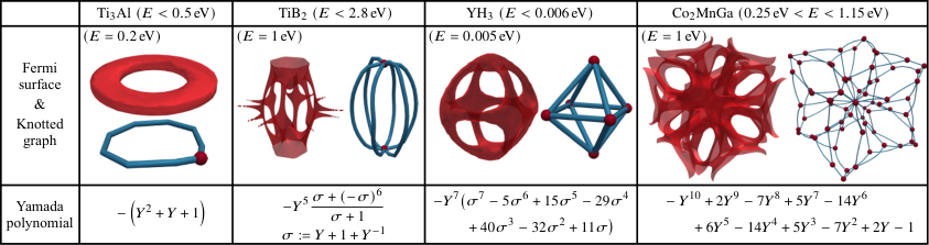
With this boundary-resolved framework established, we now compare the resulting dispersion-level fingerprints across a broader set of real materials. For graphical clarity, Fig. 4 displays representative single-component windows from each material, while the full fingerprints, including multicomponent windows that require the Yamada-set formulation, are detailed in Appendix G. The first row shows their Fermi surfaces together with the extracted knotted graphs at the indicated Fermi energies, while the second row shows the corresponding Yamada polynomials. From left to right, these are a single torus-like pocket (Ti₃Al [53]), symmetry-organized multi-tube surfaces (TiB₂ [47, 54, 48]), an octahedral skeleton motif (YH₃ [55, 56, 57]), and a highly connected multi-component structure (Co₂MnGa [46, 58, 59, 60]). The Yamada sequences of these material Hamiltonians (Appendix G) provide a systematic theoretical map of the Lifshitz transitions expected under Fermi-level tuning. Consequently, they furnish a compact topological guide to the associated changes in the density of states, transport properties, and other experimentally accessible observables. This connection opens new avenues for understanding how the intrinsic connectivity of the Fermi surface governs measurable electronic signatures. Beyond these individual Fermi surface fingerprints, we next show how the same framework resolves continuous topological evolution under microscopic deformations of both model and realistic material Hamiltonians.

2.4 Phase Diagram of Knotted Graph Topology

We next ask how an energy-resolved topological fingerprint evolves when the Hamiltonian itself is deformed, which gives a broader view of the intricate topological structures revealed by our knotted graph framework. As a minimal example, we interpolate between the unknot and Hopf-link nodal Hamiltonians:

H_{\lambda}=(1-\lambda)\,H_{\mathrm{Unknot}}+\lambda\,H_{\mathrm{Hopf}},\qquad\lambda\in[0,1],

(6)

where $H_{\mathrm{Unknot}}$ and $H_{\mathrm{Hopf}}$ are given by Eqs. 3 and 4.

Such interpolations model the continuous band-structure changes driven by experimental tuning parameters under which the evolving Hamiltonian takes the form $H_{\mathrm{mat}}(\mathbf{k};\lambda)=\sum_{a}c_{a}\!\left[\lambda\right]O_{a}(\mathbf{k})$ , with fixed operators $O_{a}(\mathbf{k})$ encoding the momentum, orbital, or hopping structure and the coefficients $c_{a}[\lambda]$ representing parameter-dependent microscopic quantities such as hopping amplitudes, orbital energies, and spin–orbit couplings [43, 72, 38, 82, 39]. We first establish the resulting parameter-resolved topology through this minimal unknot–Hopf interpolation in Fig. 5(a), and subsequently demonstrate the same construction for the material Hamiltonians of TiB₂ and Co₂MnGa in Fig. 5(b,c).

Since the unknot and Hopf link are topologically inequivalent, the $E\rightarrow 0$ Fermi surface of $H_{\lambda}$ must already possess a topological transition at some intermediate $\lambda$ . What is more interesting and unexplored is the prospect of new topological transitions across all Fermi energies $E$ , which would collectively define the topological fingerprint of its entire dispersion. At every fixed $\lambda$ , recall [see Fig. 1(c)] that we can characterize this fingerprint by the ordered Yamada sequence

\boldsymbol{\overline{\Upsilon}}(H):=\bigl[\,\overline{\Upsilon}\left(\mathcal{G}_{[1]}\right),\overline{\Upsilon}\left(\mathcal{G}_{[2]}\right),\ldots,\overline{\Upsilon}\left(\mathcal{G}_{[m]}\right)\,\bigr],

(7)

where the $\overline{\Upsilon}\!\left(\mathcal{G}_{[i]}\right)$ are the normalized Yamada polynomials for all the distinct knotted graph topologies encountered as the Fermi surface varies across the full range of $E$ . Note that $\boldsymbol{\overline{\Upsilon}}$ (boldface) is a property of the full Hamiltonian $H$ , not of any single Fermi surface or knotted graph; each entry $\overline{\Upsilon}(\mathcal{G}_{[i]})$ (non-bold) is the invariant of an individual knotted graph. For volumes with multiple boundary components, each entry is replaced by the boundary-resolved Yamada set $\overline{\Upsilon}_{\partial\mathcal{F}_{[i]}}$ in Eq. 5.

As shown in Fig. 5(a), the Fermi energy $E$ and the deformation parameter $\lambda$ define a two-dimensional topological phase space. The expected unknot to Hopf-link transition (red to green) at $\lambda\simeq 0.43$ (dashed) lives in the one-dimensional $E=0$ subspace, which bounds a much richer extended $(E,\lambda)$ phase diagram. The Lifshitz-transition boundaries marked by black curves partition it into several distinct finite-energy Fermi-surface configurations that cannot be inferred from the $E=0$ nodal slice alone.

This phase diagram can be systematically understood by examining vertical cuts at fixed $\lambda$ , starting at $E=0$ and ending at $E_{\text{max}}>1.2$ where all Fermi surfaces become topologically trivial balls. For $\lambda<0.43$ , there are only two topological configurations: a toroidal Fermi surface corresponding to the unknot (red), and a simply-connected pocket whose skeleton reduces to the isolated vertex (yellow). For $\lambda>0.43$ , the Fermi surface instead undergoes five distinct knotted graph configurations with varying $E$ : a low-energy phase with two linked toroidal components corresponding to a Hopf-link skeleton (green), which merge to form a higher-genus Fermi surface characterized by a linked-graph skeleton (purple), and subsequently a connected Fermi surface with $\theta_{3}$ -type skeleton (blue). At still higher energies, the system enters the same red unknot and yellow isolated-vertex phases encountered universally; the latter is inevitable because the Fermi surface thickens and eventually congeals into a ball as $E$ increases.

These energy-resolved topological regions provide an organizing framework for material behavior: within each energy window, the Fermi-surface topology remains fixed, whereas the boundaries between windows identify Lifshitz transitions at which Fermi-surface-sensitive observables—such as the density of states, transport coefficients, thermodynamic response, and superconducting behavior—can exhibit singularities or qualitative changes [72, 38, 39, 41, 43, 27]. The Yamada sequences [Eq. 7] listed in Fig. 5(a) provide compact labels for these distinct paths through the topological phase space. For $\lambda>0.43$ , the sequence is already given in Fig. 1(c); while for $\lambda<0.43$ it is given by

\boldsymbol{\overline{\Upsilon}}(H_{\lambda<0.43})=\bigl[-(Y^{2}+Y+1),-1\bigr].

(8)

as follows from Axioms (V) from Fig. 2. Horizontal cuts at constant $E$ instead reveal how a fixed surface topology persists under Hamiltonian deformation. At $E=0.8$ , for example, the red region extends beyond $\lambda=0.7$ , indicating that the toroidal (thickened nodal ring) topology is far more stable than what the conventional $E=0$ knot invariant suggests: while the $E\approx 0$ Fermi surface transforms from an unknot to a Hopf link at $\lambda=0.43$ , its thickened larger- $E$ counterpart remains an unknot much longer.

This parameter-resolved construction extends directly to realistic multiband Hamiltonians. In TiB₂, we vary the quartic in-plane coupling $F$ entering $h_{12}=Ck_{-}^{2}+Fk_{+}^{4}$ [Eq. 102], which controls the competition between two in-plane hybridization channels; in Co₂MnGa, we vary the momentum-dependent $d$ – $p$ hybridization coefficient $t_{8}$ entering the hybridization terms in Eq. 108. For the material phase diagrams in Fig. 5(b,c), $E$ parametrizes the interband-gap scale, as detailed in Appendix G. The resulting topology phase diagrams in Fig. 5(b,c) reveal multiple intermediate topological sectors for TiB₂ and five distinct topological sectors for Co₂MnGa, resolving how the momentum-space topology reorganizes as microscopic Hamiltonian parameters are continuously varied. Such microscopic deformations can be facilitated experimentally through tuning parameters such as strain [83], pressure [84], or composition [85]; once these controls are related to the microscopic Hamiltonian coefficients, the resulting phase maps can guide searches for Lifshitz transitions and allow experimentalists to determine where in parameter space their characteristic signatures should emerge in the density of states [72], transport [38, 39, 59, 60], thermodynamic response [41], and superconductivity [43]. The parameter paths, representative surfaces and knotted-graph skeletons, and numerical details are provided in Section G.5.

2.5 Flowed Knotted Graphs beyond Dispersion Topology: Exceptional Surfaces with Berry Curvature Flow

Having established a rigorous fermiology based on knotted graphs, we show that the framework is not limited to this setting, but adapts naturally to generic topological classifications of 2D surfaces in 3D beyond the genus. As one example, it applies to non-Hermitian band structures, specifically in symmetry-protected settings where band degeneracies are constrained to form exceptional surfaces [86, 87, 88, 70]. In the two-band case, the exceptional surface is the locus of momentum points that satisfy the band-closing condition of

H_{E}(\mathbf{k})=H(\mathbf{k})+iE\,\sigma_{y},

(9)

which is the Hamiltonian $H(k)$ of Eq. 1 subject to a gain/loss term proportional to $E$ ⁵⁵ 5 Here, the non-reciprocal $\sigma_{y}$ term is also the non-Hermitian contribution, but basis-equivalent results can be obtained even if the Pauli matrices are permuted. . Its exceptional surface is given by precisely the same condition $|f(\mathbf{k})|=E$ . Thus, our procedure given in Fig. 1(b) and the Yamada fingerprints naturally classify exceptional surfaces as well. But, as described below, exceptional surfaces are accompanied by additional topological information beyond their spatial geometry: the Berry-curvature field within them equips the corresponding knotted-graph skeleton with an intrinsic flow. Our framework can therefore be extended from classifying the exceptional surface alone to jointly characterizing its topology and the vector field supported within it.

While the full Hamiltonian remains $\mathcal{PT}$ symmetric, its eigenstates spontaneously break this symmetry inside the exceptional surface, where the eigenvalues form a complex-conjugate pair. For a chosen nondegenerate band of $H_{E}$ , let $|u^{R}\rangle$ and $\langle u^{L}|$ be the right and left eigenstates, normalized by $\langle u^{L}|u^{R}\rangle=1$ . Their biorthogonal Berry curvature is $\boldsymbol{\Omega}=i\nabla_{\mathbf{k}}\times\langle u^{L}|\nabla_{\mathbf{k}}u^{R}\rangle$ , which becomes singular on approaching the exceptional surface [70] (Appendix E). Its net flux through a cross section of each tubular branch defines a natural edge orientation, which we later prove to be an Abelian edge flow, thus producing a flowed knotted graph as illustrated in Fig. 6.

Flux conservation within the enclosed region then imposes the Kirchhoff-type vertex condition $\sum_{i=1}^{N}\Phi_{i}=0$ , where $\Phi_{i}:=\iint_{D_{i}}\boldsymbol{\Omega}(\mathbf{k})\cdot d\mathbf{S}_{i}$ is the biorthogonal Berry-curvature flux through a transverse section $D_{i}$ of the $i$ -th incident tube, with $d\mathbf{S}_{i}$ oriented outward from the vertex [see Eqs. 47 and 52]. These fluxes carry information about the eigenstate geometry beyond the eigenenergy dispersions. Accordingly, the edge orientations are not arbitrary labels: the vertex condition restricts the admissible flow patterns and determines how the Berry-curvature flux is distributed among branches meeting at a vertex. Whereas the ordinary Yamada fingerprint characterizes the underlying undirected knotted graph, the flowed graph additionally retains how the Berry-curvature flux is routed through its branches.

To demonstrate concretely that the flow carries information beyond the dispersion, we construct an isospectral pair of Hamiltonians $H_{E}^{(1)}$ and $H_{E}^{(2)}=\sigma_{x}[H_{E}^{(1)}]^{T}\sigma_{x}$ that share the same complex spectrum, exceptional surface, and unflowed skeleton, yet have everywhere opposite biorthogonal Berry curvatures $\boldsymbol{\Omega}_{1}^{\text{LR}}=-\boldsymbol{\Omega}_{2}^{\text{LR}}$ (Fig. 6). Their flowed knotted graphs are $(\mathcal{G},\varphi)$ and $(\mathcal{G},-\varphi)$ —a distinction invisible to any dispersion-based or unflowed-graph invariant. The flow therefore constitutes a joint spectral–eigenstate fingerprint: the unflowed graph $\mathcal{G}$ captures the exceptional-volume embedding determined by the eigenvalues, while the signed flow $\varphi$ captures the Berry-curvature geometry of the biorthogonal eigenstates (see Section E.3 for details).

More broadly, the flowed knotted graphs connect to the notion of Abelian $A$ -flows [90], and further flowed-graph invariants (e.g., quandle/cocycle constructions) may refine exceptional-surface fingerprints with flux information invisible to undirected invariants, with potential applications to knotted vortex tubes [91, 92, 93] and magnetic flux ropes [94, 95].

3 Discussion

We have developed a knotted-graph framework that provides a rigorous, dispersion-level topological fingerprint for generic electronic materials and beyond. Introducing knotted graphs and their Yamada polynomial invariants into fermiology already establishes a classification language far richer than conventional knot-theoretic or genus-based approaches. On top of this, applying the framework to realistic Fermi surfaces required going beyond the existing mathematical literature: the Fermi volumes of real materials generically possess multiple connected components and nested inner boundaries—compression bodies, not handlebodies—which existing Yamada polynomials cannot encode. To overcome this, we proved a new compression-body equivalence theorem, formulated boundary-wise knotted graph data, and introduced the Yamada set, enabling the first systematic Yamada-polynomial fingerprinting of real materials. The framework even further extends to surfaces endowed with vector fields: in non-Hermitian systems, the biorthogonal Berry curvature equips the knotted-graph skeleton with an Abelian edge flow, and this flow captures eigenstate geometry that is entirely invisible to the complex spectrum alone or to any unflowed-graph invariant.

Looking ahead, a natural mathematical direction is to determine whether other embedding-sensitive spatial-graph invariants can be extended to compression bodies through representative sets analogous to the Yamada set, and whether such constructions provide more discriminating or computationally efficient descriptions of their spatial topology. In particular, the same boundary-resolved construction suggests analogous Yokota- and Thompson-polynomial sets, providing alternative compression-body fingerprints with different invariance and computational properties. The cycle structure of flowed spatial graphs may further organize inequivalent Berry-flux integration paths with distinct topological roles in higher-dimensional parameter spaces where the corresponding fluxes can become quantized. Moreover our construction naturally motivates the broader notion of flowed compression bodies, in which a vector field or directional structure carried by the embedded region is represented through corresponding sets of oriented or flow-carrying spatial graphs, enabling the joint characterization of spatial embedding and physically relevant flow structure. At a still more global level, the evolving 1D knotted graph generated as the Fermi energy is swept traces a 2D knotted surface in the extended $(3+1)$ -dimensional momentum–energy space. Describing the full dispersion as a single embedded surface therefore offers a complementary formulation that may connect the present framework to surface-knot theory, including 2-knots in appropriate closed cases, and capture global topological information across the complete energy evolution. This perspective also raises an inverse problem: given a Yamada sequence, or more generally an energy-resolved sequence of spatial-topological invariants, what constraints does it impose on the class of compatible dispersions, and can candidate band structures or Hamiltonians be reconstructed directly from such data?

A broader application-oriented direction is to develop this framework into a scalable methodology for systematically characterizing realistic electronic structures across materials, energies and experimentally accessible control parameters. Further optimization of graph extraction, invariant evaluation and phase-space tracking could enable high-throughput integration with DFT and Wannier-based workflows, allowing Lifshitz transitions and changes in Fermi-surface connectivity and spatial entanglement to be identified across large material and parameter spaces. At the materials-database scale, Yamada sequences and related spatial-topological descriptors could provide compact fingerprints for comparing materials, identifying robust and recurring topological structures, and screening for candidate systems with targeted Fermi-surface connectivity, Berry-flux structure or Lifshitz-transition behavior. More broadly, such a high-throughput topological description could enable systematic investigation of how momentum-space topology correlates with material properties across large material families, providing a route toward identifying topology–property relationships and using them to guide materials discovery.

Acknowledgments

This research is supported by the Singapore Ministry of Education (MOE) through the Academic Research Fund Tier-II Grant MOE-T2EP50224-0007. During the preparation of this manuscript, the authors used ChatGPT and Claude to assist with language refinement and the revision of selected passages originally drafted by the authors. All AI-assisted revisions were reviewed and edited by the authors, who take full responsibility for the final content.

Data and Code Availability

All data and code associated with this work are available from the corresponding authors upon reasonable request.

References

[1] S. Ryu, A. P. Schnyder, A. Furusaki, and A. W. W. Ludwig, New Journal of Physics 12, 065010 (2010).
[2] A. P. Schnyder, S. Ryu, A. Furusaki, and A. W. W. Ludwig, Phys. Rev. B 78, 195125 (2008).
[3] C.-K. Chiu, J. C. Y. Teo, A. P. Schnyder, and S. Ryu, Rev. Mod. Phys. 88, 035005 (2016).
[4] D. Vanderbilt, Berry phases in electronic structure theory: electric polarization, orbital magnetization and topological insulators (Cambridge University Press, 2018).
[5] R. Bi, Z. Yan, L. Lu, and Z. Wang, Physical Review B 96, 10.1103/physrevb.96.201305 (2017).
[6] Z. Yan, R. Bi, H. Shen, L. Lu, S.-C. Zhang, and Z. Wang, Physical Review B 96, 10.1103/physrevb.96.041103 (2017).
[7] L. Li, C. H. Lee, and J. Gong, Physical review letters 121, 036401 (2018).
[8] M. Stålhammar, L. Rødland, G. Arone, J. C. Budich, and E. Bergholtz, SciPost Physics 7, 10.21468/scipostphys.7.2.019 (2019).
[9] L. Li, C. H. Lee, and J. Gong, Communications Physics 2, 135 (2019).
[10] J. Carlström, M. Stålhammar, J. C. Budich, and E. J. Bergholtz, Phys. Rev. B 99, 161115(R) (2019).
[11] C. H. Lee, A. Sutrisno, T. Hofmann, T. Helbig, Y. Liu, Y. S. Ang, L. K. Ang, X. Zhang, M. Greiter, and R. Thomale, Nature Communications 11, 10.1038/s41467-020-17716-1 (2020a).
[12] Y. S. S. Patil, J. Höller, P. A. Henry, C. Guria, Y. Zhang, L. Jiang, N. Kralj, N. Read, and J. G. E. Harris, Nature 607, 271–275 (2022).
[13] T. Tai and C. H. Lee, Phys. Rev. B 107, L220301 (2023).
[14] R. Lin, T. Tai, L. Li, and C. H. Lee, Frontiers of Physics 18, 10.1007/s11467-023-1309-z (2023).
[15] F. Qin, R. Shen, L. Li, and C. H. Lee, Physical Review A 109, 053311 (2024).
[16] Z. Yang, K. Zhang, C. Fang, and J. Hu, Physical Review Letters 125, 226402 (2020a).
[17] Q. Li, H. Jiang, and C. H. Lee, Advanced Science 12, e08047 (2025).
[18] D. Gu, Z. Fu, Y.-M. Hu, and Z. Wang, arXiv preprint arXiv:2608.28577 (2026).
[19] M. Yang, A. N. Poddubny, and C. H. Lee, arXiv preprint arXiv:2608.02746 (2026a).
[20] Y. Xiong and H. Hu, Phys. Rev. B 109, L100301 (2024).
[21] J. Pi, C. Wang, Y.-C. Liu, and Y. Yan, Physical Review B 111, 10.1103/physrevb.111.165407 (2025).
[22] X. Yan, H. Akgün, K. Kawaguchi, N. D. Loh, and C. H. Lee, Hsg-12m: A large-scale spatial multigraph dataset (2025), arXiv:2506.08618 [cs.LG] .
[23] P. Sala, T. Rakovszky, R. Verresen, M. Knap, and F. Pollmann, Phys. Rev. X 10, 011047 (2020).
[24] V. Khemani, M. Hermele, and R. Nandkishore, Phys. Rev. B 101, 174204 (2020).
[25] I. Lifshitz et al., Sov. Phys. JETP 11, 1130 (1960).
[26] Y. M. Blanter, M. Kaganov, A. Pantsulaya, and A. Varlamov, Physics Reports 245, 159 (1994).
[27] A. A. Varlamov, Y. M. Galperin, S. G. Sharapov, and Y. Yerin, Low Temperature Physics 47, 672–683 (2021).
[28] R. Franzosi, M. Pettini, and L. Spinelli, Physical Review Letters 84, 2774–2777 (2000).
[29] S. Biasotti, D. Giorgi, M. Spagnuolo, and B. Falcidieno, Theoretical Computer Science 392, 5 (2008), computational Algebraic Geometry and Applications.
[30] M. C. Gibson, A. B. Patel, R. Nagpal, and N. Perrimon, Nature 442, 1038 (2006).
[31] W. T. Gibson and M. C. Gibson, in Current Topics in Developmental Biology, Current Topics in Developmental Biology, Vol. 89 (Academic Press, 2009) pp. 87–114.
[32] A. L. Melott, Physics Reports 193, 1 (1990).
[33] C. J. Copi, D. P. Mihaylov, A. Negro, A. Samandar, G. D. Starkman, Y. Akrami, G. Alestas, S. Anselmi, J. C. Duque, F. Cornet-Gomez, L. H. Lu, A. H. Jaffe, A. Kosowsky, M. M. Barandiaran, T. S. Pereira, C. Petretti, and A. Tamosiunas, The topology of the universe (2026), arXiv:2606.24886 [astro-ph.CO] .
[34] A. Hatcher, Algebraic topology (Cambridge University Press, 2002).
[35] The genus only captures the topological connectivity of the surface of the 3D structure, not how its 3D “bulk” is embedded.
[36] H. Edelsbrunner and J. Harer, in Surveys on Discrete and Computational Geometry: Twenty Years Later, Contemporary Mathematics, Vol. 453 (American Mathematical Society, 2008) pp. 257–282.
[37] G. Carlsson, Bulletin of the American mathematical society 46, 255 (2009).
[38] S. Galeski, H. F. Legg, R. Wawrzyńczak, T. Förster, S. Zherlitsyn, D. Gorbunov, M. Uhlarz, P. M. Lozano, Q. Li, G. D. Gu, C. Felser, J. Wosnitza, T. Meng, and J. Gooth, Nature Communications 13, 10.1038/s41467-022-35106-7 (2022).
[39] Y. Zhang, C. Wang, L. Yu, G. Liu, A. Liang, J. Huang, S. Nie, X. Sun, Y. Zhang, B. Shen, J. Liu, H. Weng, L. Zhao, G. Chen, X. Jia, C. Hu, Y. Ding, W. Zhao, Q. Gao, C. Li, S. He, L. Zhao, F. Zhang, S. Zhang, F. Yang, Z. Wang, Q. Peng, X. Dai, Z. Fang, Z. Xu, C. Chen, and X. J. Zhou, Nature Communications 8, 10.1038/ncomms15512 (2017).
[40] Y. Zhong, Z. Chen, S.-D. Chen, K.-J. Xu, M. Hashimoto, Y. He, S. ichi Uchida, D. Lu, S.-K. Mo, and Z.-X. Shen, Proceedings of the National Academy of Sciences 119, e2204630119 (2022), https://www.pnas.org/doi/pdf/10.1073/pnas.2204630119 .
[41] S. Slizovskiy, A. V. Chubukov, and J. J. Betouras, Phys. Rev. Lett. 114, 066403 (2015).
[42] D. Kang, Y. Zhou, W. Yi, C. Yang, J. Guo, Y. Shi, S. Zhang, Z. Wang, C. Zhang, S. Jiang, A. Li, K. Yang, Q. Wu, G. Zhang, L. Sun, and Z. Zhao, Nature Communications 6, 10.1038/ncomms8804 (2015).
[43] X. Shi, Z.-Q. Han, X.-L. Peng, P. Richard, T. Qian, X.-X. Wu, M.-W. Qiu, S. C. Wang, J. P. Hu, Y.-J. Sun, and H. Ding, Nature Communications 8, 10.1038/ncomms14988 (2017).
[44] G. E. Volovik, Physics–Uspekhi 61, 89 (2018).
[45] J. Y. Lin, N. C. Hu, Y. J. Chen, C. H. Lee, and X. Zhang, Physical Review B , 075438 (2017).
[46] G. Chang, S.-Y. Xu, X. Zhou, S.-M. Huang, B. Singh, B. Wang, I. Belopolski, J. Yin, S. Zhang, A. Bansil, H. Lin, and M. Z. Hasan, Phys. Rev. Lett. 119, 156401 (2017).
[47] X. Feng, C. Yue, Z. Song, Q. Wu, and B. Wen, Phys. Rev. Mater. 2, 014202 (2018).
[48] C.-J. Yi, B. Q. Lv, Q. S. Wu, B.-B. Fu, X. Gao, M. Yang, X.-L. Peng, M. Li, Y.-B. Huang, P. Richard, M. Shi, G. Li, O. V. Yazyev, Y.-G. Shi, T. Qian, and H. Ding, Phys. Rev. B 97, 201107 (2018).
[49] Y. Xie, J. Cai, J. Kim, P.-Y. Chang, and Y. Chen, Physical Review B 99, 10.1103/physrevb.99.165147 (2019).
[50] G. Ding, T. Sun, and X. Wang, Physical Chemistry Chemical Physics 24, 11175 (2022).
[51] Q. Yan, R. Liu, Z. Yan, B. Liu, H. Chen, Z. Wang, and L. Lu, Nature Physics 14, 461–464 (2018).
[52] E. Yang, B. Yang, O. You, H.-C. Chan, P. Mao, Q. Guo, S. Ma, L. Xia, D. Fan, Y. Xiang, and S. Zhang, Physical Review Letters 125, 10.1103/physrevlett.125.033901 (2020b).
[53] X. Zhang, Z.-M. Yu, Z. Zhu, W. Wu, S.-S. Wang, X.-L. Sheng, and S. A. Yang, Physical Review B 97, 235150 (2018).
[54] Z. Liu, R. Lou, P. Guo, Q. Wang, S. Sun, C. Li, S. Thirupathaiah, A. Fedorov, D. Shen, K. Liu, H. Lei, and S. Wang, Phys. Rev. X 8, 031044 (2018).
[55] D. Shao, T. Chen, Q. Gu, Z. Guo, P. Lu, J. Sun, L. Sheng, and D. Xing, Scientific Reports 8, 10.1038/s41598-018-19870-5 (2018).
[56] J. Huiberts, J. Rector, R. Wijngaarden, S. Jetten, D. De Groot, B. Dam, N. Koeman, R. Griessen, B. Hjörvarsson, S. Olafsson, et al., Journal of Alloys and Compounds 239, 158 (1996).
[57] Y. Wang and M. Chou, Physical Review B 51, 7500 (1995).
[58] I. Belopolski, K. Manna, D. S. Sanchez, G. Chang, B. Ernst, J. Yin, S. S. Zhang, T. Cochran, N. Shumiya, H. Zheng, B. Singh, G. Bian, D. Multer, M. Litskevich, X. Zhou, S.-M. Huang, B. Wang, T.-R. Chang, S.-Y. Xu, A. Bansil, C. Felser, H. Lin, and M. Z. Hasan, Science 365, 1278 (2019), https://www.science.org/doi/pdf/10.1126/science.aav2327 .
[59] S. N. Guin, K. Manna, J. Noky, S. J. Watzman, C. Fu, N. Kumar, W. Schnelle, C. Shekhar, Y. Sun, J. Gooth, and C. Felser, NPG Asia Materials 11, 10.1038/s41427-019-0116-z (2019).
[60] A. Markou, D. Kriegner, J. Gayles, L. Zhang, Y.-C. Chen, B. Ernst, Y.-H. Lai, W. Schnelle, Y.-H. Chu, Y. Sun, and C. Felser, Phys. Rev. B 100, 054422 (2019).
[61] J. H. Conway and C. M. Gordon, Journal of Graph Theory 7, 445 (1983).
[62] L. H. Kauffman, Transactions of the American Mathematical Society 311, 697 (1989).
[63] E. Flapan, T. W. Mattman, B. Mellor, R. Naimi, and R. Nikkuni, in Knots, Links, Spatial Graphs, and Algebraic Invariants, Contemporary Mathematics, Vol. 689 (American Mathematical Society, 2017) pp. 81–102.
[64] In the mathematics literature, knotted graphs are usually called spatial graphs.
[65] J. W. Alexander, Transactions of the American Mathematical Society 30, 275 (1928).
[66] V. F. Jones, Bulletin of the American Mathematical Society 12, 103 (1985).
[67] J. Hoste, M. Thistlethwaite, and J. Weeks, The Mathematical Intelligencer 20, 33 (1998).
[68] D. Rolfsen, Knots and links, AMS Chelsea Publishing, Vol. 346 (American Mathematical Society, 2003).
[69] E. J. Bergholtz, J. C. Budich, and F. K. Kunst, Reviews of Modern Physics 93, 015005 (2021).
[70] P. Wang, L. Jin, and Z. Song, Phys. Rev. B 109, 115406 (2024).
[71] V. G. Bardakov and D. A. Fedoseev, Invariants of handlebody-links and spatial graphs (2025), arXiv:2504.09718 [math.GT] .
[72] S. Ichinokura, M. Toyoda, M. Hashizume, K. Horii, S. Kusaka, S. Ideta, K. Tanaka, R. Shimizu, T. Hitosugi, S. Saito, and T. Hirahara, Phys. Rev. B 105, 235307 (2022).
[73] The nodal set at $E=0$ is just the locus $\{\mathbf{k}\in\text{BZ}:f(\mathbf{k})=0\}$ .
[74] B. Bode and M. R. Dennis, Constructing a polynomial whose nodal set is any prescribed knot or link (2016), arXiv:1612.06328 [math.GT] .
[75] B. Bode, M. R. Dennis, D. Foster, and R. P. King, Proceedings of the Royal Society A: Mathematical, Physical and Engineering Sciences 473, 20160829 (2017).
[76] X. Zhang, G. Li, Y. Liu, T. Tai, R. Thomale, and C. H. Lee, Communications Physics 4, 47 (2021).
[77] S. Yamada, Journal of Graph Theory 13, 537 (1989).
[78] B. Mellor, Invariants of Spatial Graphs (2018), arXiv:1812.08885 [math] .
[79] The unnormalized Yamada polynomial $\Upsilon$ is invariant under moves (II)–(IV), corresponding to regular rigid-vertex isotopy. Its normalized form $\overline{\Upsilon}$ removes the monomial factors associated with moves (I) and (V) and is therefore invariant under moves (I)–(V), corresponding to rigid-vertex isotopy. Ambient isotopy additionally permits edge reordering at vertices through move (VI). If all vertices have degree $\leq 3$ —as is the case for every example in Fig. 2— $\overline{\Upsilon}$ is consequently a full ambient-isotopy invariant. For graphs containing higher-degree vertices, which do arise for the real materials in Appendix G, we use the minimum-crossing planar-projection convention detailed in Appendix D.
[80] W. Kohn, A. D. Becke, and R. G. Parr, The Journal of Physical Chemistry 100, 12974 (1996).
[81] A. Kormányos, G. Burkard, M. Gmitra, J. Fabian, V. Zólyomi, N. D. Drummond, and V. Fal’ko, 2D Materials 2, 022001 (2015).
[82] Y. Wu, N. H. Jo, M. Ochi, L. Huang, D. Mou, S. L. Bud’ko, P. C. Canfield, N. Trivedi, R. Arita, and A. Kaminski, Phys. Rev. Lett. 115, 166602 (2015).
[83] V. Sunko, E. Abarca Morales, I. Marković, M. E. Barber, D. Milosavljević, F. Mazzola, D. A. Sokolov, N. Kikugawa, C. Cacho, P. Dudin, H. Rosner, C. W. Hicks, P. D. C. King, and A. P. Mackenzie, npj Quantum Materials 4, 46 (2019).
[84] Z. J. Xiang, G. J. Ye, C. Shang, B. Lei, N. Z. Wang, K. S. Yang, D. Y. Liu, F. B. Meng, X. G. Luo, L. J. Zou, Z. Sun, Y. Zhang, and X. H. Chen, Physical Review Letters 115, 10.1103/physrevlett.115.186403 (2015).
[85] P. Dziawa, B. J. Kowalski, K. Dybko, R. Buczko, A. Szczerbakow, M. Szot, E. Łusakowska, T. Balasubramanian, B. M. Wojek, M. H. Berntsen, O. Tjernberg, and T. Story, Nature Materials 11, 1023–1027 (2012).
[86] S.-B. Yang, P.-R. Han, W. Ning, F. Wu, Z.-B. Yang, and S.-B. Zheng, Science China Physics, Mechanics & Astronomy 69, 230313 (2026b).
[87] M. Stålhammar and E. J. Bergholtz, Physical Review B 104, L201104 (2021).
[88] K. Kawabata, T. Bessho, and M. Sato, Physical Review Letters 123, 066405 (2019).
[89] Here, the non-reciprocal $\sigma_{y}$ term is also the non-Hermitian contribution, but basis-equivalent results can be obtained even if the Pauli matrices are permuted.
[90] A. Ishii and M. Iwakiri, Canadian Journal of Mathematics 64, 102 (2012).
[91] R. L. Ricca and M. A. Berger, Physics Today 49, 28 (1996).
[92] D. Kleckner and W. Irvine, Nature Physics 9, 253 (2013).
[93] D. Kleckner, L. H. Kauffman, and W. T. Irvine, Nature Physics 12, 650 (2016).
[94] R. Liu, Research in Astronomy and Astrophysics 20, 165 (2020).
[95] P. M. Bellan, Physics of Plasmas 10, 1999–2008 (2003).
[96] Y. Yokota, Topology 35, 77 (1996).
[97] A. Thompson, Topology 31, 657 (1992).
[98] Y. Huh, Yamada polynomial and associated link of $\theta$ -curves (2022), arXiv:2206.11450 [math.GT] .
[99] S. Negami, Transactions of the American Mathematical Society 299, 601 (1987).
[100] A. Ishii, Algebraic & Geometric Topology 8, 1403 (2008).
[101] R. S. Vennila, E. E. Porchelvi, K. M. F. Joy, T. K. J. Arun, and N. V. Jaya, Journal of Alloys and Compounds 392, 24 (2005).
[102] S.-J. Chen, Y. Chen, H. Zhang, Y. Tang, J.-j. Wei, and W.-g. Sun, Journal of Nanomaterials 2013, 1 (2013).
[103] A single vertex is a bouquet of zero circles, i.e., $\mathcal{B}_{0}$ .
[104] C. H. Lee, H. H. Yap, T. Tai, G. Xu, X. Zhang, and J. Gong, Physical Review B 102, 10.1103/physrevb.102.035138 (2020b).
[105] T. Tai and C. H. Lee, Physical Review B 103, 195125 (2021).
[106] L. Kauffman, J. Simon, K. Wolcott, and P. Zhao, Topology and its Applications 49, 193 (1993).
[107] K. Kuratowski, Fundamenta Mathematicae 15, 271 (1930).
[108] K. Wagner, Mathematische Annalen 114, 570 (1937).
[109] M. R. Fellows and M. A. Langston, Journal of the ACM 35, 727 (1988).
[110] J. Nešetřil and R. Thomas, Commentationes Mathematicae Universitatis Carolinae 26, 655 (1985).
[111] H. Sachs, in Graph Theory, Lecture Notes in Mathematics, Vol. 1018, edited by M. Borowiecki, J. W. Kennedy, and M. M. Syso (Springer, Berlin, Heidelberg, 1983).
[112] H. Sachs, in Finite and Infinite Sets, Vols. I and II, Colloq. Math. Soc. Jańos Bolyai, Vol. 37, edited by A. Hajnal, L. Lovász, and V. T. Soś (North Holland, Amsterdam, New York, 1984) pp. 649–662.
[113] N. Robertson, P. Seymour, and R. Thomas, Journal of Combinatorial Theory, Series B 64, 185 (1995).
[114] E. Flapan, R. Naimi, and J. Pommersheim, Topology and its Applications 115, 239 (2001a).
[115] G. Bowlin and J. Foisy, Journal of Knot Theory and its Ramifications 13, 1021 (2004).
[116] E. Flapan, J. Pommersheim, J. Foisy, and R. Naimi, Journal of Knot Theory and its Ramifications 10, 1143 (2001b).
[117] R. Naimi, in Encyclopedia of Knot Theory (Chapman and Hall/CRC, 2021) pp. 467–476.
[118] J. Foisy, Journal of Graph Theory 39, 178 (2002).
[119] B. Johnson, M. E. Kidwell, and T. S. Michael, Journal of Knot Theory and Its Ramifications 19, 10.1142/S0218216510008455 (2010).
[120] J. Barsotti and T. W. Mattman, Involve, a Journal of Mathematics 9, 591 (2016).
[121] H. Kim, T. Mattman, and S. Oh, Journal of Knot Theory and Its Ramifications 27, 1850059 (2018).
[122] P. Blain, G. Bowlin, T. Fleming, J. Foisy, J. Hendricks, and J. LaCombe, Journal of Knot Theory and its Ramifications 16, 749 (2007).
[123] M. Ozawa and Y. Tsutsumi, Revista Matemática Complutense 20, 391 (2007).
[124] J. Miller and R. Naimi, Experimental Mathematics 23, 6 (2014).
[125] H. Choi, H. Kim, and S. No, Discrete Applied Mathematics 291, 237 (2021).
[126] H. Choi, H. Kim, and S. No, Chirality for simple graphs of size up to 12 (2022), arXiv:2208.09241 [math.GT] .
[127] E. Flapan and W. Fletcher, Intrinsic chirality of multipartite graphs (2013), arXiv:1303.5131 [math.GT] .
[128] E. Flapan and N. Weaver, Proceedings of the American Mathematical Society 115, 233 (1992), accessed 15 Apr. 2025.
[129] B. Bode, Topology and its Applications 243, 33–51 (2018).

Supplemental Material

The supplemental material collects a glossary overview, computational details, invariant constructions, and extended results that support the main text. They cover the skeletonization pipeline, Yamada polynomial evaluation, multi-boundary compression-body generalization and Yamada set, additional Yamada sequences for real materials, and other pure graph-theoretic signatures such as planarity and intrinsic linkedness.

Appendix A Glossary

•

Brillouin zone (BZ). Momentum space of a 3D lattice. Under periodic boundary condition it is topologically a 3-torus, $T^{3}$ .
•

Constant-energy surface / Fermi surface (level set). For a chosen band $n$ with dispersion $\varepsilon_{n}(\mathbf{k})$ , the constant-energy surface at Fermi energy $E$ is $\Sigma_{E}^{(n)}:=\{\mathbf{k}\in\mathrm{BZ}:\varepsilon_{n}(\mathbf{k})=E\}$ . This is equivalently the Fermi surface at Fermi energy $E$ . When $E$ is a regular value of $\varepsilon_{n}$ , $\Sigma_{E}^{(n)}$ is a smooth embedded closed surface, possibly with several connected components and nested inner boundaries. In the main text, after choosing one representative energy in the $i$ -th window whose two ends are Lifshitz transitions, we denote the corresponding surface topology by $\Sigma_{[i]}$ (or in general $\Sigma_{[i]}^{(n)}$ with explicit band label).
•

Fermi sea / Fermi volume (sublevel set). We use “Fermi volume” as shorthand for the enclosed sublevel region $\mathcal{F}_{E}^{(n)}:=\{\mathbf{k}\in\mathrm{BZ}:\varepsilon_{n}(\mathbf{k})\leq E\}$ . For regular $E$ , it is a compact 3-manifold with boundary $\partial\mathcal{F}_{E}^{(n)}=\Sigma_{E}^{(n)}$ . A generic Fermi volume may have multiple disjoint components and each possibly with nested inner boundaries, in which case we analyze the volume boundary-wise. Once a representative energy is selected in the $i$ -th window, we write $\mathcal{F}_{[i]}$ or $\mathcal{F}_{[i]}^{(n)}$ to represent the topological equivalent (homeomorphic) Fermi volume.
•

Handlebody. A compact, connected, orientable three-manifold obtained by attaching 1-handles to a 3-ball. Equivalently, it is the regular neighborhood of an embedded graph. Fermi volumes in Fig. 1 are precisely handlebodies. A handlebody up to homeomorphism is in one-to-one correspondence with its embedded knotted graph up to ambient isotopy and contraction moves (Appendix F).
•

Compression body. A multiply-connected generalization of a handlebody with a distinguished outer boundary $\partial_{+}$ and possibly several inner boundaries (voids) $\partial_{-}$ (Fig. S14). A generic Fermi volume is a compression body having multiple boundaries, and thus generic Fermi surface is multi-component. This extension beyond handlebodies is necessary to characterize the realistic Fermi surfaces that arise in the materials considered in this study.
•

Knotted graph (Spatial graph). An embedding of an abstract graph into a three-manifold (here the Brillouin zone $BZ\cong T^{3}$ ). Two such embeddings are considered the same when they can be connected by ambient isotopy and contraction moves, unless stated otherwise. In the math literature [90, 71], the embedded graph onto which a handlebody deformation-retracts is also called a spine; different spines of the same handlebody are related by ambient isotopy together with contraction/expansion moves (Whitehead moves).
•

Skeleton graph. The specific knotted graph obtained by our numerical skeletonization procedure (Appendix C)—a “canonical” representative of the equivalence class of knotted graphs associated with a given Fermi volume. We denote it by $\mathcal{G}_{[i]}$ or $\mathcal{G}_{[i]}^{(n)}$ for the $i$ -th window and $n$ -th band. In practice, it is obtained by topology-preserving thinning and pruning of a voxelized Fermi volume. For compression-body components with inner boundaries, the corresponding invariants are recorded boundary-wise through the Yamada-set construction.
•

Planar diagram (Spatial-graph diagram). A generic projection of a spatial graph to $\mathbb{R}^{2}$ , in which vertices project to distinct points, edge intersections away from vertices are crossings (in math term, transverse double points), and each crossing carries over/under information. Thus a planar diagram is a diagrammatic encoding of a spatial embedding (not the same thing as a crossing-free planar embedding of the abstract graph). Generalized Reidemeister moves and Yamada polynomial are defined in terms of planar diagrams (2D projections), not directly in terms of 3D embeddings. Throughout this manuscript, we denote the diagram of the spatial graph $\mathcal{G}$ by the same notation $\mathcal{G}$ for brevity.
•

Generalized Reidemeister moves. The local moves (I)–(VI) on planar diagrams of spatial graphs. Moves (I)–(III) are the usual knot/link Reidemeister moves, while moves (IV)–(VI) involve graph vertices. Moves (I)–(V) generate rigid (flat) vertex isotopy; adding move (VI) gives pliable vertex isotopy (i.e. ambient isotopy).
•

Ambient isotopy / Pliable vertex isotopy. A continuous deformation of the ambient three-manifold (here $BZ\cong T^{3}$ ) carrying one embedded graph to another. In diagrammatic terms, this is the equivalence generated by generalized Reidemeister moves (I)–(VI).
•

Rigid-vertex isotopy. An isotopy in which the cyclic order of the half-edges at each vertex is fixed. Diagrammatically, it is generated by moves (I)–(V); move (VI) is excluded because it can change that cyclic order.
•

Yamada polynomial and its normalization. The Yamada polynomial $\Upsilon(\mathcal{G};Y)$ is a one-variable Laurent polynomial defined by the axioms in Table S2, with $\sigma:=Y+1+Y^{-1}$ . The unnormalized polynomial is invariant under regular rigid-vertex isotopy, i.e. under moves (II)–(IV). We use the normalized form $\overline{\Upsilon}(\mathcal{G};Y)$ , which removes the monomial factors from moves (I) and (V) so that $\overline{\Upsilon}$ is invariant under moves (I)–(V). In general it is not invariant under move (VI); however, if all vertices have degree at most $3$ , then move (VI) is generated by moves (I,IV,V), hence $\overline{\Upsilon}$ is also an ambient-isotopy invariant in this case.
•

Yamada set (multi-boundary invariant). For a generic Fermi surface with multiple boundaries in the $i$ -th energy window of band $n$ , we record the multiset of normalized Yamada polynomials associated with each boundary, $\overline{\Upsilon}_{\partial\mathcal{F}_{[i]}^{(n)}}:=\{\overline{\Upsilon}(\mathcal{G}_{[i],\alpha}^{(n)};Y)\}_{\alpha=1}^{m_{[i]}^{(n)}}$ , where $\alpha$ runs over all boundary components of $\mathcal{F}_{[i]}^{(n)}$ . This boundary-wise encoding generalizes the single Yamada polynomial that is appropriate only for handlebody.
•

Yamada sequence. For a Hamiltonian $H$ , the Yamada sequence is the ordered list of invariants encountered across successive energy windows. If $E_{1}<\cdots<E_{m+1}$ are consecutive Lifshitz energies and one representative energy is chosen in each window $E\in(E_{i},E_{i+1})$ , then in the handlebody case $\boldsymbol{\overline{\Upsilon}}(H)=\bigl[\overline{\Upsilon}(\mathcal{G}_{[1]}),\ldots,\overline{\Upsilon}(\mathcal{G}_{[m]})\bigr]$ . For generic multi-boundary Fermi surface (Fermi volume being compression-body), the $i$ -th entry is the corresponding multiset-valued Yamada set $\overline{\Upsilon}_{\partial\mathcal{F}_{[i]}}$ . In other words, a Yamada sequence is a sequence of Yamada sets, and reduces to a sequence of Yamada polynomials in the handlebody case.
•

Lifshitz transition. The change of Fermi surface topology at a critical energy. I.e., as $E$ crosses a critical value of $\varepsilon_{n}$ , and the Fermi volume changes by a standard Morse-theoretic move such as handle attachment/removal or component merger/splitting. Meanwhile it implies that the Fermi surface crosses at least one van Hove singularity $\mathbf{k}:\nabla_{\mathbf{k}}\varepsilon_{n}=0$ . In semiclassical language, the Fermi velocity is the flow field on the Fermi surface, van Hove singularities are its zeros, and a Lifshitz transition means crossing a van Hove point. Thus, Lifshitz transition is associated with the global reorganization of Fermi velocity field on the Fermi surface.
•

Exceptional surface. For the perturbed non-Hermitian two-band model $H_{E}(\mathbf{k})=H(\mathbf{k})+iE\,\sigma_{y}$ (Eq. 9) (note $E$ here is the perturbation strength parameter, not the constant-energy), the exceptional surface is the momentum set where $H_{E}$ becomes defective.
•

Biorthogonal Berry connection and curvature. Let the right/left eigenvectors for a non-Hermitian band be $|u_{n}^{R}(\mathbf{k})\rangle$ and $\langle u_{n}^{L}(\mathbf{k})|$ , normalized biorthogonally by $\langle u_{n}^{L}|u_{n}^{R}\rangle=1$ ; $n$ is the band index. The Berry connection and curvature are $\mathbf{A}_{n}(\mathbf{k})=i\langle u_{n}^{L}|\nabla_{\mathbf{k}}|u_{n}^{R}\rangle$ and $\boldsymbol{\Omega}_{n}(\mathbf{k})=\nabla_{\mathbf{k}}\times\mathbf{A}_{n}(\mathbf{k})$ .
•

Abelian edge flow. An assignment $\phi$ of values in an Abelian group $A$ to oriented edges of a graph such that reversing the orientation reverses the value, $\phi(\bar{e})=-\phi(e)$ , and the signed sum of incident edge values vanishes at each vertex (Kirchhoff junction rule). In our exceptional surface example, the flow on a knotted-graph edge is defined by the Berry flux $\Phi_{B}\in\mathbb{R}$ flowing through the tube cross-section, and thus the Abelian group is the additive real numbers $A=(\mathbb{R},+)$ .

Appendix B Ansatzes of Nodal Hamiltonians and their Fermi Surfaces

Many of the illustrative knotted graph and Yamada polynomial fingerprints in the main text are based on the Fermi surface of the two-band nodal-knot Hamiltonian ansatz Eq. 1 [5, 9]:

H(\mathbf{k})=[\mathrm{Re}\,f(\mathbf{k})]\,\sigma_{x}+[\mathrm{Im}\,f(\mathbf{k})]\,\sigma_{z},

(10)

whose dispersion relation is

\varepsilon_{\pm}(\mathbf{k})=\pm|f(\mathbf{k})|,

(11)

with $f(\mathbf{k})$ constructed from the two building blocks $z(\mathbf{k}),w(\mathbf{k})$ defined in Eq. 2:

	$\displaystyle z(\mathbf{k})$	$\displaystyle=\cos(2k_z)+\tfrac{1}{2}+i\bigl(\cos k_{x}+\cos k_{y}+\cos k_{z}-2\bigr)$
	$\displaystyle w(\mathbf{k})$	$\displaystyle=\sin k_{x}+i\,\sin k_{y}$		(12)

A key advantage of this ansatz is that desired knot topologies can be straightforwardly designed: by construction, it generates a family of Hamiltonians with nodal sets at $E=0$ forming knots, links, and knotted graphs—namely, the nodal knot / nodal link / nodal graph.

Nodal set type	Ansatz $f(z,w)$ in Hamiltonian [Eq. 1]
Unknot	$z$
Hopf link	$z^{2}-w^{2}$
Trefoil knot	$z^{2}-w^{3}$
Solomon’s knot	$z^{2}-w^{4}$
Cinquefoil knot	$z^{2}-w^{5}$
Three-link	$z(z^{2}-w^{2})$
$(p,q)$ -torus knot	$z^{p}-w^{q}$
Awesome knotted graph (a fine-tuned nodal graph)	$z(z^{2}-w^{4}+w)$

Table S1: Ansatzes of nodal knots/links/graphs used in this work. The nodal set at

E=0

is given by

f(z(\mathbf{k}),w(\mathbf{k}))=0

, while Fermi surfaces are

|f(\mathbf{k})|=E

Table S1 lists some functional forms of $f(z,w)$ and the corresponding nodal set types. Fig. S7 shows some of the nodal sets and overlays their Fermi surfaces at various Fermi energies.

For these models, the Fermi surfaces of the positive band at $E$ are the level sets

\Sigma_{E}=\{\mathbf{k}\in\mathrm{BZ}:|f(\mathbf{k})|=E\},

(13)

and in the nodal limit $E=0$ the knotted graph reduces to $\mathcal{G}_{[1]}\cong\Sigma_{(E=0)}$ —the nodal knot/link/graph itself.

Appendix C Computational Skeletonization Pipeline

This section explains our numerical method that maps a Fermi surface to its knotted graph used for topological classification.

C.1 From Fermi sea to skeleton graph

For a chosen band $n$ and Fermi energy $E$ , we start from the Fermi surface $\Sigma_{E}^{(n)}=\{\mathbf{k}\in\mathrm{BZ}:\varepsilon_{n}(\mathbf{k})=E\}$ in the Brillouin zone. After selecting one representative energy in the $i$ -th interval between Lifshitz transitions, we denote this surface by $\Sigma_{[i]}$ or $\Sigma_{[i]}^{(n)}$ . For regular $E$ , the surface is smooth and embedded. Topology changes occur only at critical energies (Lifshitz transitions), where the level set becomes singular and components merge, split, or change genus through handle attachment/removal.

For our purposes, the surface topology is most conveniently represented through its enclosed region. We therefore take the sublevel set, i.e., the Fermi sea or Fermi volume, as input:

\mathcal{F}_{E}^{(n)}=\{\mathbf{k}\in\mathrm{BZ}:\varepsilon_{n}(\mathbf{k})\leq E\},

(14)

and deterministically extract a 1D skeleton graph $\mathcal{G}_{[i]}^{(n)}$ from it.

This volume-based method is numerically more stable than trying to infer graph connectivity directly from a surface triangulation, and it also matches the conceptual picture of handlebody used throughout the paper.

This is the progression illustrated in Fig. S8. At $E=0$ , the Fermi surface collapses to the nodal knot itself. At finite Fermi energy, the level set thickens into a surface bounding a Fermi volume, and Lifshitz transitions can create additional necks and handles. The computational task is then to collapse that volume to a graph that captures its topology.

The pipeline summarized in Fig. S8(b–d) is: (i) voxelize the enclosed volume on a 3D grid; (ii) apply topology-preserving thinning to obtain a 1-voxel-thick skeleton; (iii) convert the remaining skeleton voxels into vertices and edges; and (iv) prune artifacts that do not affect the Fermi topology. The result is the embedded graph $\mathcal{G}_{[i]}^{(n)}$ used in the subsequent Yamada-polynomial computation.

C.2 Medial axis as an “innermost” skeleton

The thinning step is motivated by the “medial-axis” conceptual picture in Fig. S9. For a solid region $V\subset\mathbb{R}^{3}$ , the medial axis is the set of points that have more than one closest point on the closed boundary $\partial V$ . Equivalently, it is the set of centers of maximal inscribed balls in $V$ . Informally, it is the most “interior” center set of the volume.

For a generic 3D object, the medial axis can contain 2D sheets (usually when geometry is symmetric), so it is not necessarily always 1D. These 2D medial-axis sheets are geometrically meaningful, but they are more detailed than what is needed for the topological invariant used in our analysis. For topological classification, we merely need a skeleton that preserves the connected components and tunnels of the volume. Thus, more precisely, our thinning procedure is a topology-preserving collapse inspired by the medial axis: in practice, we perform iterative thinning that also collapses sheet-like parts of the medial-axis to a 1D skeleton.

C.3 Practical pipeline: iterative morphological thinning and graph pruning

We begin by voxelizing the Fermi volume on a regular 3D grid: first discretize the Brillouin zone into a 3D grid of small cubes (voxels), then mark each voxel as inside or outside $\mathcal{F}_{E}^{(n)}$ .

We then iteratively remove boundary voxels that are simple in the sense of digital topology. Deleting a simple voxel leaves both the occupied voxel set and its complement with the same connectivity, so no components, tunnels, or cavities are created or destroyed. The iteration stops when no further simple boundary voxels remain. The result is a topology-preserving 1-voxel-thick skeleton.

This “raw” skeleton is not yet the graph used for invariants. It typically contains short spurious spurs caused by discretization noise, as well as topology-wise redundant degree-two vertices scattered along otherwise smooth edges.

To obtain a clean spatial graph, we propose and implement two pruning steps:

•

Trim short degree-one spurs (“bristles”). Remove short degree-one branches up to a certain length threshold. These short spurs are artifacts of numeric noise, and they are irrelevant to the cycle structure that encodes the underlying knot/link/graph topology. In geometric topology, this equivalence-preserving operation is known as contraction; the inverse operation of this is expansion which adds leaf edges. However, we do keep long leaf edges in the output, as they carry physical information rather than being voxel-scale noise.
•

Remove degree-two vertices. Degree-two vertices are also irrelevant to the spatial graph topology; they only appear when a spatial edge has sharp twists, which is identified by our skeleton-to-graph program as a turning vertex. Removing degree-two vertices is equivalent to merging consecutive edge segments into a single edge. In geometric topology, this equivalence-preserving operation is known as un-subdivision, whose inverse is subdivision that adds degree-two vertices on edges. This yields a minimal embedded graph of interest and significantly reduces numeric overhead for invariant computation (e.g., the Yamada polynomial) without changing the ambient-isotopy class of the knotted graph.

After these topological simplification steps, the resulting graph, denoted by $\mathcal{G}_{[i]}$ , is the knotted graph fingerprint that is used throughout this work.

Appendix D Yamada Polynomial — Definition, Property, and Efficient evaluation

[Uncaptioned image] — Table S2: Generalized Reidemeister moves and Yamada polynomial. (left) generalized Reidemeister moves for spatial graph diagrams. The usual Reidemeister moves (I–III) govern knot ambient isotopy (highlighted with a green box); the additional vertex moves (IV–VI) generalize the conventional moves, and in conjuntion with moves (I–III), they govern the ambient isotopy of spatial graph (highlighted with a blue box). (middle) defining axioms (including skein relations) of Yamada polynomial $\Upsilon(\mathcal{G};Y)$ . These axioms define a “raw” Yamada polynomial that is invariant up to moves (II,III,IV), namely, regular rigid vertex isotopy. (right) additional formulae that constrains $\Upsilon$ and normalizes $\Upsilon\to\overline{\Upsilon}$ , such that it is invariant up to moves (I–V), namely, rigid vertex isotopy. If the maximum degree of the vertices is 3 or less, e.g. conventional knots/links, and all examples in Fig. 2(a–f), $\overline{\Upsilon}(\mathcal{G};Y)$ becomes invariant up to all moves (I–VI) and thus it’s an invariant of ambient isotopy (or pliable vertex isotopy, or simply isotopy). The normalized $\overline{\Upsilon}$ is reported consistently throughout this work, if not stated otherwise.

In conventional knot theory, knots and links are studied as a planar diagram, i.e. a direct projection from 3D embedding to 2D plane $\mathbb{R}^{2}$ (see an example in Fig. S11). Knot’s ambient isotopy is governed by the conventional Reidemeister moves (I–III) [Table S2 (left, green box)], which are defined and operate on the planar diagram. Topological invariants e.g. Alexander polynomial can effectively distinguish non-isotopic knots.

Knotted-graphs (spatial-graphs), which are much less commonly known, similarly have graph diagrams, which in additional allow vertices (of arbitrary degree). Knotted-graph’s ambient isotopy is in turn governed by the generalized Reidemeister moves (I–VI) [78, 62] [Table S2 (left, blue box)].

To account for the additional vertex moves (IV–VI), knot invariants are generalized to invariants of knotted graphs that capture both knot-theoretic and graph-theoretic structure. The best-known such invariant is the Yamada polynomial [77]. The definition and evaluation reviewed in this section are standard [77, 78, 62]; our extensions beyond existing literature—the compression-body framework, Yamada set, and Yamada sequence—are developed in Appendix F and applied to real materials in Appendix G.

For readers familiar with knot theory, the Yamada polynomial $\Upsilon(Y)$ for knotted graphs plays a role analogous to the Alexander polynomial $\mathcal{A}(A)$ for ordinary knots and links. In the nodal regime $E\gtrsim 0$ prior to the first Lifshitz transition, the skeleton of the Fermi surface forms an ordinary knot or link, which can be classified using conventional knot invariants; examples of Alexander polynomials are shown in Fig. S10(a,d,g,j). Once Lifshitz transitions occur and vertices appear on the skeleton graph, however, it leaves the class of knots and enters the broader class of knotted graphs, illustrated in Fig. S10(b,c,e,f,h,i,k,l). Knot-only invariants are then no longer applicable, whereas the Yamada polynomial continues to apply.

Equivalently, knots can be viewed as a special subset of knotted graphs. In that sense, the Yamada polynomial naturally extends the scope of knot invariants: it applies to ordinary knots/links when no vertices are present, and it remains applicable after vertices appear. This is the main reason it is the appropriate invariant for the family of spines studied in this work, as it covers both the nodal knot limit and all the connectivity changes due to Lifshitz transitions in a unified way.

D.1 Definition, normalization, and properties

The Yamada polynomial is defined purely by local skein relations Table S2(middle)—recursive relations on graph diagrams. An efficient algorithmic way to compute the Yamada polynomial is through a state-sum, namely by resolving crossings into planar states. We discuss the definition, properties, and state-sum evaluation of the Yamada polynomial in order next.

The unnormalized Yamada polynomial can be defined as the unique Laurent polynomial $\Upsilon(\mathcal{G};Y)$ that satisfies the axioms in Table S2(middle).

Starting from these axioms, it can be shown that the Laurent polynomial is unchanged under moves (II), (III), and the rigid-vertex move (IV). In mathematical language unnormalized Yamada polynomial is an invariant of spatial graphs up to regular rigid vertex isotopy.

Generally, the moves (I), (V) or (VI) would change the unnormalized $\Upsilon(\mathcal{G};Y)$ . In particular, moves (I) and (V) change the polynomial by multiplying a monomial of $(-Y)$ ; the behavior is summarized as the first two formulae in Table S2(right). Following this convention, we can remove the dependence on moves (I,V) by normalizing the polynomial:

\boxed{\overline{\Upsilon}(\mathcal{G};Y):=(-Y)^{-m}\,\Upsilon(\mathcal{G};Y),\qquad m:=\min\{\text{exponents of }Y\text{ appearing in }\Upsilon(\mathcal{G};Y)\}}

(15)

This normalized $\overline{\Upsilon}(\mathcal{G};Y)$ is an invariant of rigid vertex isotopy, i.e., invariance under moves (I–V).

An important special scenario is that, for graphs with maximum vertex degree $\leq 3$ , move (VI) can be decomposed into moves (V) $\to$ (IV,I). Hence, $\overline{\Upsilon}$ is an ambient isotopy invariant in these cases [78]. E.g., for conventional knots/links, and all examples in Fig. 2(a–f), $\overline{\Upsilon}$ is an ambient isotopy invariant. Ambient isotopy is also known as pliable vertex isotopy, or simply isotopy.

Convention for graphs with higher-degree vertices.

When $\mathcal{G}$ has a vertex of degree $\geq 4$ , move (VI) is no longer generated by moves (I–V), and $\overline{\Upsilon}$ is only a rigid vertex isotopy invariant: two diagrams of the same embedded graph that differ by a cyclic reordering of the edges around such a vertex may yield different $\overline{\Upsilon}$ . Such vertices do occur in this work—the real-material skeletons of Appendix G contain vertices of degree up to $6$ (in $\theta_{6}$ ) and $12$ (in $\theta_{12,P}$ ). To fix a definite diagram in these cases, we adopt a minimum-crossing planar-projection convention: among the generic planar projections of the embedded graph, we retain one whose diagram realizes the smallest crossing number, and quote the $\overline{\Upsilon}$ of that diagram. In practice we keep the projection plane fixed to be the $xy$ plane and rotate the embedded graph instead. A generic rotation carries three Euler angles, but the third one merely rotates the resulting diagram within the projection plane, and reversing the viewing direction (a flip of the $z$ axis) only shows the same diagram from behind. Since neither operation changes the diagram obtained, the genuinely distinct projections are labelled by a viewing direction taken up to antipodal identification, i.e. by one half of the direction sphere, over which we sample uniformly. We draw $N_{\mathrm{rot}}$ such rotations ( $N_{\mathrm{rot}}=10$ by default), project each rotated graph onto the $xy$ plane, and evaluate $\overline{\Upsilon}$ on whichever of the resulting diagrams carries the fewest crossings. We do not prove that this sampling is guaranteed to reach a globally unique minimum-crossing polynomial for an arbitrary knotted graph; we only observe that the attained minimum already saturates at $N_{\mathrm{rot}}=10$ for every knotted graph appearing in this manuscript. A selection procedure with an accompanying guarantee is left for future work. Whenever every vertex has degree $\leq 3$ , no such choice is needed and the projection may be taken arbitrarily.

Relatedly, other ambient-isotopy invariants also exist (e.g., the Yokota polynomial [96] and Thompson polynomial [97]), but they are typically much more expensive to evaluate.

D.2 State-sum evaluation via the specialized Negami polynomial

A practical way to compute the Yamada polynomial is through a state-sum expansion [98]. One starts from a planar diagram of a spatial graph $\mathcal{G}$ , namely a 2D projection together with the over/under-crossing information. At each crossing , the skein relation in Table S2(middle) yields three local resolutions: the two smoothings and , and the vertex resolution . After resolving every crossing, one obtains a crossing-free planar graph, called a state. Here “planar graph” means that the resulting graph can be drawn in the plane without any remaining edge intersections; do not conflate it with “planar diagram”. If the original diagram has $c$ crossings, then there are $3^{c}$ possible states.

Let $S$ be the set of all such states. For a given state $s\in S$ , denote by $\mathcal{G}_{s}$ the planar graph obtained after all crossings are resolved. Let $p(s)$ and $m(s)$ be the numbers of and smoothings used in the construction of $s$ , respectively; the remaining crossings are resolved by . The Yamada polynomial is then obtained as the weighted sum over all states:

\boxed{\Upsilon(\mathcal{G};Y)=\sum_{s\in S}Y^{p(s)-m(s)}\,h\!\left(\mathcal{G}_{s};\,-1,\,-Y-2-Y^{-1}\right)}

(16)

This formula separates the problem into two steps: first resolve the crossings, and then evaluate a purely graph-theoretic quantity on the resulting planar graphs.

For a crossing-free graph $\mathcal{G}_{s}$ , the required two-variable polynomial $h(\mathcal{G}_{s};x,y)$ is the specialization of the Negami polynomial used in Yamada’s construction [99]:

h(\mathcal{G}_{s};x,y)=\sum_{F\subseteq E(\mathcal{G}_{s})}(-x)^{-|F|}\,x^{\mu(\mathcal{G}_{s}-F)}\,y^{\beta(\mathcal{G}_{s}-F)},

(17)

where $F$ is a subset of edges to be deleted, $\mathcal{G}_{s}-F$ is the graph obtained after deleting those edges, and $\sum_{F\subseteq E(\mathcal{G}_{s})}$ sums over all possible edge subsets. $\mu(\mathcal{G}_{s}-F)$ is the number of connected components of the remaining graph, and $\beta(\mathcal{G}_{s}-F)$ is its first Betti number, also called the cycle rank, which counts the number of independent cycles. In the Yamada specialization $x=-1$ , the prefactor $(-x)^{-|F|}$ becomes unity, so the contribution of each deleted-edge configuration is controlled only by the topology of the remaining graph through $\mu$ and $\beta$ .

For graphs, the first Betti number can be computed from the Euler–Poincaré relation,

\beta(\mathcal{G}_{s}-F)=|E(\mathcal{G}_{s}-F)|-|V(\mathcal{G}_{s})|+\mu(\mathcal{G}_{s}-F),

(18)

where $|E(\mathcal{G}_{s}-F)|$ and $|V(\mathcal{G}_{s})|=|V(\mathcal{G}_{s}-F)|$ are the numbers of edges and vertices, respectively. Thus, once a state has been produced, its contribution can be computed entirely from standard combinatorial data of the planar graph, and thereby the Yamada polynomial can be expressed in terms of planar graphs and their standard combinatorial data:

\boxed{\Upsilon(\mathcal{G};Y)=\sum_{s\in S}Y^{p(s)-m(s)}\,\sum_{F\subseteq E(\mathcal{G}_{s})}\,(-1)^{\mu(\mathcal{G}_{s}-F)}\,(-Y-2-Y^{-1})^{|E(\mathcal{G}_{s}-F)|-|V(\mathcal{G}_{s})|+\mu(\mathcal{G}_{s}-F)}}

(19)

In summary, the state-sum method converts the 3D topological problem into a sum over crossing resolutions, with each resolved state evaluated by a specialized graph polynomial, although the state space scales exponentially with the crossing number.

Notably, this state-sum procedure enables us to construct an algorithmic pipeline to compute the Yamada polynomial, significantly expanding our investigation scope of our topological fingerprinting framework beyond the limits of manual computation.

D.3 Worked example: a two-crossing diagram

We now illustrate the state-sum procedure on a minimal nontrivial example. We consider the knotted graph extracted from the Fermi surface $\Sigma_{[2]}$ of the Hopf-link Hamiltonian at $E=0.3$ shown in Fig. 1(c), whose knotted graph is now displayed separately in Fig. S11(a). Because this graph is trivalent, the normalized polynomial $\overline{\Upsilon}$ is an ambient-isotopy invariant, so any projection angle may be used. We choose the projection shown in Fig. S11(b).

The projected diagram has 4 vertices, 6 edges, and 2 crossings. Note that the crossings are not graph vertices; in math language, they are called transverse double points, the point where two edges overlap in the projection and which one goes over the other is important information.

Since each crossing admits three local resolutions, the diagram generates $3^{2}=9$ planar states, displayed in Fig. S11(c). For each state $s$ , the contribution to the un-normalized Yamada polynomial is [Eq. 19]:

Y^{p(s)-m(s)}\,h\!\left(\mathcal{G}_{s};-1,-Y-2-Y^{-1}\right)=Y^{p(s)-m(s)}\sum_{F\subseteq E(\mathcal{G}_{s})}(-1)^{\mu(\mathcal{G}_{s}-F)}(-Y-2-Y^{-1})^{|E(\mathcal{G}_{s}-F)|-|V(\mathcal{G}_{s})|+\mu(\mathcal{G}_{s}-F)},

Once a state is fixed, the problem is purely graph-theoretic: one only needs the number of connected components $\mu$ and the Betti-1 number $\beta=|E|-|V|+\mu$ for the graphs obtained by deleting subsets of edges.

As an explicit example of how to compute one state, consider the state obtained by choosing the $\bigl(\scalebox{0.7}{\hbox to29.95pt{\vbox to29.95pt{\pgfpicture\makeatletter\hbox{\hskip 14.97638pt\lower-14.97638pt\hbox to0.0pt{\lxSVG@begingroup@{_scopebegin=1} \lxSVG@begingroup@{stroke=#000000} \lxSVG@begingroup@{fill=#000000} \lxSVG@setlinewidth{\the\pgflinewidth}\lxSVG@begingroup@{stroke-width=0.4pt} \lx@inpgf@ignorespaces\nullfont\hbox to0.0pt{\lxSVG@begingroup@{_scopebegin=1} {{\lx@inpgf@ignorespaces}}\lxSVG@setlinewidth{\the\pgflinewidth}\lxSVG@begingroup@{stroke-width=1.5pt} \lx@inpgf@ignorespaces{{}{{}}{} {{\lx@inpgf@ignorespaces}{}\lx@inpgf@ignorespaces}{{}} {{{}}{{\lx@inpgf@ignorespaces}}}{{}}{{{}}{{}}}{}{{}}{}{}{}\lxSVG@begingroup@{_scopebegin=1} \color[rgb]{1,0,0}{}\lxSVG@stroke\lxSVG@drawpath@unclipped{M 19.69 -19.69 C 19.69 1.81 -19.69 1.81 -19.69 -19.69}{fill:none} \lx@inpgf@ignorespaces \lxSVG@closescope {}{{}}{} {{\lx@inpgf@ignorespaces}{}\lx@inpgf@ignorespaces}{{}} {{{}}{{\lx@inpgf@ignorespaces}}}{{}}{{{}}{{}}}{}{{}}{}{}{}\lxSVG@begingroup@{_scopebegin=1} \color[rgb]{0,0,1}{}\lxSVG@stroke\lxSVG@drawpath@unclipped{M -19.69 19.69 C -19.69 -1.81 19.69 -1.81 19.69 19.69}{fill:none} \lx@inpgf@ignorespaces \lxSVG@closescope } \lxSVG@closescope {\lx@inpgf@ignorespaces}{\lx@inpgf@ignorespaces}{\lx@inpgf@ignorespaces}\hss}\lxSVG@discardpath\lxSVG@closescope \hss}}\lxSVG@closescope\endpgfpicture}}},\scalebox{0.7}{\hbox to29.95pt{\vbox to29.95pt{\pgfpicture\makeatletter\hbox{\hskip 14.97638pt\lower-14.97638pt\hbox to0.0pt{\lxSVG@begingroup@{_scopebegin=1} \lxSVG@begingroup@{stroke=#000000} \lxSVG@begingroup@{fill=#000000} \lxSVG@setlinewidth{\the\pgflinewidth}\lxSVG@begingroup@{stroke-width=0.4pt} \lx@inpgf@ignorespaces\nullfont\hbox to0.0pt{\lxSVG@begingroup@{_scopebegin=1} {{\lx@inpgf@ignorespaces}}\lxSVG@setlinewidth{\the\pgflinewidth}\lxSVG@begingroup@{stroke-width=1.5pt} \lx@inpgf@ignorespaces{{}{{}}{} {{\lx@inpgf@ignorespaces}{}\lx@inpgf@ignorespaces}{{}} {{{}}{{\lx@inpgf@ignorespaces}}}{{}}{{{}}{{}}}{}{{}}{}{}{}\lxSVG@begingroup@{_scopebegin=1} \color[rgb]{1,0,0}{}\lxSVG@stroke\lxSVG@drawpath@unclipped{M 19.69 -19.69 C 19.69 1.81 -19.69 1.81 -19.69 -19.69}{fill:none} \lx@inpgf@ignorespaces \lxSVG@closescope {}{{}}{} {{\lx@inpgf@ignorespaces}{}\lx@inpgf@ignorespaces}{{}} {{{}}{{\lx@inpgf@ignorespaces}}}{{}}{{{}}{{}}}{}{{}}{}{}{}\lxSVG@begingroup@{_scopebegin=1} \color[rgb]{0,0,1}{}\lxSVG@stroke\lxSVG@drawpath@unclipped{M -19.69 19.69 C -19.69 -1.81 19.69 -1.81 19.69 19.69}{fill:none} \lx@inpgf@ignorespaces \lxSVG@closescope } \lxSVG@closescope {\lx@inpgf@ignorespaces}{\lx@inpgf@ignorespaces}{\lx@inpgf@ignorespaces}\hss}\lxSVG@discardpath\lxSVG@closescope \hss}}\lxSVG@closescope\endpgfpicture}}}\bigr)$ resolution pair in Fig. S11(c), i.e. the center one in the diagram matrix.

The resulting planar, crossing-free graph is a disjoint union of two $\theta_{3}$ -graph (two vertices connected by three parallel edges constitute a $\theta_{3}$ -graph). Similar to the axiom (III) in Table S2(middle), Negami polynomial has a similar skein relation for disjoint unions of graphs:

h\bigl(\scalebox{0.4}{\hbox to29.95pt{\vbox to29.95pt{\pgfpicture\makeatletter\hbox{\hskip 14.97638pt\lower-14.97638pt\hbox to0.0pt{\lxSVG@begingroup@{_scopebegin=1} \lxSVG@begingroup@{stroke=#000000} \lxSVG@begingroup@{fill=#000000} \lxSVG@setlinewidth{\the\pgflinewidth}\lxSVG@begingroup@{stroke-width=0.4pt} \lx@inpgf@ignorespaces\nullfont\hbox to0.0pt{\lxSVG@begingroup@{_scopebegin=1} {{\lx@inpgf@ignorespaces}}\lxSVG@setlinewidth{\the\pgflinewidth}\lxSVG@begingroup@{stroke-width=1.5pt} \lx@inpgf@ignorespaces{{}{{}}{} {{\lx@inpgf@ignorespaces}{}\lx@inpgf@ignorespaces}{{}} {{{}}{{\lx@inpgf@ignorespaces}}}{{}}{{{}}{{}}}{}{{}}{}{}{}\lxSVG@begingroup@{_scopebegin=1} \color[rgb]{1,0,0}{}\lxSVG@stroke\lxSVG@drawpath@unclipped{M 19.69 -19.69 C 19.69 1.81 -19.69 1.81 -19.69 -19.69}{fill:none} \lx@inpgf@ignorespaces \lxSVG@closescope {}{{}}{} {{\lx@inpgf@ignorespaces}{}\lx@inpgf@ignorespaces}{{}} {{{}}{{\lx@inpgf@ignorespaces}}}{{}}{{{}}{{}}}{}{{}}{}{}{}\lxSVG@begingroup@{_scopebegin=1} \color[rgb]{0,0,1}{}\lxSVG@stroke\lxSVG@drawpath@unclipped{M -19.69 19.69 C -19.69 -1.81 19.69 -1.81 19.69 19.69}{fill:none} \lx@inpgf@ignorespaces \lxSVG@closescope } \lxSVG@closescope {\lx@inpgf@ignorespaces}{\lx@inpgf@ignorespaces}{\lx@inpgf@ignorespaces}\hss}\lxSVG@discardpath\lxSVG@closescope \hss}}\lxSVG@closescope\endpgfpicture}}},\scalebox{0.4}{\hbox to29.95pt{\vbox to29.95pt{\pgfpicture\makeatletter\hbox{\hskip 14.97638pt\lower-14.97638pt\hbox to0.0pt{\lxSVG@begingroup@{_scopebegin=1} \lxSVG@begingroup@{stroke=#000000} \lxSVG@begingroup@{fill=#000000} \lxSVG@setlinewidth{\the\pgflinewidth}\lxSVG@begingroup@{stroke-width=0.4pt} \lx@inpgf@ignorespaces\nullfont\hbox to0.0pt{\lxSVG@begingroup@{_scopebegin=1} {{\lx@inpgf@ignorespaces}}\lxSVG@setlinewidth{\the\pgflinewidth}\lxSVG@begingroup@{stroke-width=1.5pt} \lx@inpgf@ignorespaces{{}{{}}{} {{\lx@inpgf@ignorespaces}{}\lx@inpgf@ignorespaces}{{}} {{{}}{{\lx@inpgf@ignorespaces}}}{{}}{{{}}{{}}}{}{{}}{}{}{}\lxSVG@begingroup@{_scopebegin=1} \color[rgb]{1,0,0}{}\lxSVG@stroke\lxSVG@drawpath@unclipped{M 19.69 -19.69 C 19.69 1.81 -19.69 1.81 -19.69 -19.69}{fill:none} \lx@inpgf@ignorespaces \lxSVG@closescope {}{{}}{} {{\lx@inpgf@ignorespaces}{}\lx@inpgf@ignorespaces}{{}} {{{}}{{\lx@inpgf@ignorespaces}}}{{}}{{{}}{{}}}{}{{}}{}{}{}\lxSVG@begingroup@{_scopebegin=1} \color[rgb]{0,0,1}{}\lxSVG@stroke\lxSVG@drawpath@unclipped{M -19.69 19.69 C -19.69 -1.81 19.69 -1.81 19.69 19.69}{fill:none} \lx@inpgf@ignorespaces \lxSVG@closescope } \lxSVG@closescope {\lx@inpgf@ignorespaces}{\lx@inpgf@ignorespaces}{\lx@inpgf@ignorespaces}\hss}\lxSVG@discardpath\lxSVG@closescope \hss}}\lxSVG@closescope\endpgfpicture}}}\bigr)=h\bigl(\raisebox{-5.59721pt}{\scalebox{0.4}{\hbox to56.17pt{\vbox to40.63pt{\pgfpicture\makeatletter\hbox{\hskip 27.88345pt\lower-69.908pt\hbox to0.0pt{\lxSVG@begingroup@{_scopebegin=1} \lxSVG@begingroup@{stroke=#000000} \lxSVG@begingroup@{fill=#000000} \lxSVG@setlinewidth{\the\pgflinewidth}\lxSVG@begingroup@{stroke-width=0.4pt} \lx@inpgf@ignorespaces\nullfont\hbox to0.0pt{\lxSVG@begingroup@{_scopebegin=1} {{\lx@inpgf@ignorespaces}}{{}{{}}{} {}{{}}{}{}{}{}{{}}{}\lx@inpgf@ignorespaces {{}}\lx@inpgf@ignorespaces\hbox{\hbox{{\lxSVG@begingroup@{_scopebegin=1} \lxSVG@begingroup@{stroke=#000000} \lxSVG@begingroup@{fill=#FF0000} {{}{{{}}}{{}}{}{}{\lx@inpgf@ignorespaces}{\lx@inpgf@ignorespaces}{}{}{}{}{}{\lxSVG@begingroup@{_scopebegin=1} \lxSVG@begingroup@{stroke=#000000} \lxSVG@begingroup@{fill=#FF0000} {}\lxSVG@fillstroke\lxSVG@drawpath@unclipped{M -19.44 -68.9 C -19.44 -62.89 -24.31 -58.02 -30.31 -58.02 C -36.32 -58.02 -41.19 -62.89 -41.19 -68.9 C -41.19 -74.9 -36.32 -79.77 -30.31 -79.77 C -24.31 -79.77 -19.44 -74.9 -19.44 -68.9 Z M -30.31 -68.9}{} \lx@inpgf@ignorespaces \lxSVG@closescope }{{{{\lx@inpgf@ignorespaces}}\lxSVG@begingroup@{_scopebegin=1} \lxSVG@transformcm{1.0}{0.0}{0.0}{1.0}{-25.92665pt}{-52.8796pt}\lxSVG@begingroup@{transform=matrix(1.0 0.0 0.0 1.0 -35.87 -73.17)} \pgfsys@hbox{64}\lxSVG@closescope }}} \lxSVG@closescope }}} {{}}\lx@inpgf@ignorespaces\hbox{\hbox{{\lxSVG@begingroup@{_scopebegin=1} \lxSVG@begingroup@{stroke=#000000} \lxSVG@begingroup@{fill=#FF0000} {{}{{{}}}{{}}{}{}{\lx@inpgf@ignorespaces}{\lx@inpgf@ignorespaces}{}{}{}{}{}{\lxSVG@begingroup@{_scopebegin=1} \lxSVG@begingroup@{stroke=#000000} \lxSVG@begingroup@{fill=#FF0000} {}\lxSVG@fillstroke\lxSVG@drawpath@unclipped{M 40.99 -68.9 C 40.99 -63 36.21 -58.23 30.31 -58.23 C 24.42 -58.23 19.64 -63 19.64 -68.9 C 19.64 -74.79 24.42 -79.57 30.31 -79.57 C 36.21 -79.57 40.99 -74.79 40.99 -68.9 Z M 30.31 -68.9}{} \lx@inpgf@ignorespaces \lxSVG@closescope }{{{{\lx@inpgf@ignorespaces}}\lxSVG@begingroup@{_scopebegin=1} \lxSVG@transformcm{1.0}{0.0}{0.0}{1.0}{18.12466pt}{-52.8796pt}\lxSVG@begingroup@{transform=matrix(1.0 0.0 0.0 1.0 25.08 -73.17)} \pgfsys@hbox{64}\lxSVG@closescope }}} \lxSVG@closescope }}} {{}}{}{{}} {{{{{}}{}{}{}{}{{}}}}}{}{{{{{}}{}{}{}{}{{}}}}}{{}}{}{}{}{\lxSVG@begingroup@{_scopebegin=1} \lxSVG@begingroup@{_scopebegin=1} \lxSVG@begingroup@{stroke=#000000} \lxSVG@setlinewidth{\the\pgflinewidth}\lxSVG@begingroup@{stroke-width=3.0pt} \lx@inpgf@ignorespaces{}\lxSVG@stroke\lxSVG@drawpath@unclipped{M -19.16 -68.9 L 19.37 -68.9}{fill:none} \lx@inpgf@ignorespaces \lxSVG@closescope \lxSVG@closescope }\lxSVG@begingroup@{_scopebegin=1} \lxSVG@begingroup@{stroke=#0000FF} \lxSVG@setlinewidth{\the\pgflinewidth}\lxSVG@begingroup@{stroke-width=1.5pt} \lx@inpgf@ignorespaces{}\lxSVG@stroke\lxSVG@drawpath@unclipped{M -19.16 -68.9 L 19.37 -68.9}{fill:none} \lx@inpgf@ignorespaces \lxSVG@closescope {{}}{} {\lx@inpgf@ignorespaces{}{}{{}}{}}{\lx@inpgf@ignorespaces{}{}{{}}{}}{{}{}\lx@inpgf@ignorespaces}{{}} {\lx@inpgf@ignorespaces{}{}{{}}{}}{{{}}{{}}}{{}}{\lx@inpgf@ignorespaces{}{}{{}}{}}{{{}}{{}}}{{}}{}{{}}{{{{{}}{}{}{}{}{{}}}}}{{}}{}{{{{{{}}{}{}{}{}{{}}}}}{}{}{}{}}{\lxSVG@begingroup@{_scopebegin=1} \lxSVG@begingroup@{_scopebegin=1} \lxSVG@begingroup@{stroke=#000000} \lxSVG@setlinewidth{\the\pgflinewidth}\lxSVG@begingroup@{stroke-width=3.0pt} \lx@inpgf@ignorespaces{}\lxSVG@stroke\lxSVG@drawpath@unclipped{M -30.31 -80.05 C -30.31 -103.69 30.31 -103.49 30.31 -79.84}{fill:none} \lx@inpgf@ignorespaces \lxSVG@closescope \lxSVG@closescope }\lxSVG@begingroup@{_scopebegin=1} \lxSVG@begingroup@{stroke=#0000FF} \lxSVG@setlinewidth{\the\pgflinewidth}\lxSVG@begingroup@{stroke-width=1.5pt} \lx@inpgf@ignorespaces{}\lxSVG@stroke\lxSVG@drawpath@unclipped{M -30.31 -80.05 C -30.31 -103.69 30.31 -103.49 30.31 -79.84}{fill:none} \lx@inpgf@ignorespaces \lxSVG@closescope {{}}{} {\lx@inpgf@ignorespaces{}{}{{}}{}}{\lx@inpgf@ignorespaces{}{}{{}}{}}{{}{}\lx@inpgf@ignorespaces}{{}} {\lx@inpgf@ignorespaces{}{}{{}}{}}{{{}}{{}}}{{}}{\lx@inpgf@ignorespaces{}{}{{}}{}}{{{}}{{}}}{{}}{}{{}}{{{{{}}{}{}{}{}{{}}}}}{{}}{}{{{{{{}}{}{}{}{}{{}}}}}{}{}{}{}}{\lxSVG@begingroup@{_scopebegin=1} \lxSVG@begingroup@{_scopebegin=1} \lxSVG@begingroup@{stroke=#000000} \lxSVG@setlinewidth{\the\pgflinewidth}\lxSVG@begingroup@{stroke-width=3.0pt} \lx@inpgf@ignorespaces{}\lxSVG@stroke\lxSVG@drawpath@unclipped{M -30.31 -57.74 C -30.31 -34.1 30.31 -34.31 30.31 -57.95}{fill:none} \lx@inpgf@ignorespaces \lxSVG@closescope \lxSVG@closescope }\lxSVG@begingroup@{_scopebegin=1} \lxSVG@begingroup@{stroke=#0000FF} \lxSVG@setlinewidth{\the\pgflinewidth}\lxSVG@begingroup@{stroke-width=1.5pt} \lx@inpgf@ignorespaces{}\lxSVG@stroke\lxSVG@drawpath@unclipped{M -30.31 -57.74 C -30.31 -34.1 30.31 -34.31 30.31 -57.95}{fill:none} \lx@inpgf@ignorespaces \lxSVG@closescope } \lxSVG@closescope {\lx@inpgf@ignorespaces}{\lx@inpgf@ignorespaces}{\lx@inpgf@ignorespaces}\hss}\lxSVG@discardpath\lxSVG@closescope \hss}}\lxSVG@closescope\endpgfpicture}}}}\amalg\raisebox{-5.59721pt}{\scalebox{0.4}{\hbox to56.17pt{\vbox to40.63pt{\pgfpicture\makeatletter\hbox{\hskip 27.88345pt\lower-69.908pt\hbox to0.0pt{\lxSVG@begingroup@{_scopebegin=1} \lxSVG@begingroup@{stroke=#000000} \lxSVG@begingroup@{fill=#000000} \lxSVG@setlinewidth{\the\pgflinewidth}\lxSVG@begingroup@{stroke-width=0.4pt} \lx@inpgf@ignorespaces\nullfont\hbox to0.0pt{\lxSVG@begingroup@{_scopebegin=1} {{\lx@inpgf@ignorespaces}}{{}{{}}{} {}{{}}{}{}{}{}{{}}{}\lx@inpgf@ignorespaces {{}}\lx@inpgf@ignorespaces\hbox{\hbox{{\lxSVG@begingroup@{_scopebegin=1} \lxSVG@begingroup@{stroke=#000000} \lxSVG@begingroup@{fill=#FF0000} {{}{{{}}}{{}}{}{}{\lx@inpgf@ignorespaces}{\lx@inpgf@ignorespaces}{}{}{}{}{}{\lxSVG@begingroup@{_scopebegin=1} \lxSVG@begingroup@{stroke=#000000} \lxSVG@begingroup@{fill=#FF0000} {}\lxSVG@fillstroke\lxSVG@drawpath@unclipped{M -19.59 -68.9 C -19.59 -62.97 -24.39 -58.17 -30.31 -58.17 C -36.24 -58.17 -41.04 -62.97 -41.04 -68.9 C -41.04 -74.82 -36.24 -79.63 -30.31 -79.63 C -24.39 -79.63 -19.59 -74.82 -19.59 -68.9 Z M -30.31 -68.9}{} \lx@inpgf@ignorespaces \lxSVG@closescope }{{{{\lx@inpgf@ignorespaces}}\lxSVG@begingroup@{_scopebegin=1} \lxSVG@transformcm{1.0}{0.0}{0.0}{1.0}{-25.75443pt}{-52.8796pt}\lxSVG@begingroup@{transform=matrix(1.0 0.0 0.0 1.0 -35.64 -73.17)} \pgfsys@hbox{64}\lxSVG@closescope }}} \lxSVG@closescope }}} {{}}\lx@inpgf@ignorespaces\hbox{\hbox{{\lxSVG@begingroup@{_scopebegin=1} \lxSVG@begingroup@{stroke=#000000} \lxSVG@begingroup@{fill=#FF0000} {{}{{{}}}{{}}{}{}{\lx@inpgf@ignorespaces}{\lx@inpgf@ignorespaces}{}{}{}{}{}{\lxSVG@begingroup@{_scopebegin=1} \lxSVG@begingroup@{stroke=#000000} \lxSVG@begingroup@{fill=#FF0000} {}\lxSVG@fillstroke\lxSVG@drawpath@unclipped{M 41.25 -68.9 C 41.25 -62.86 36.35 -57.97 30.31 -57.97 C 24.28 -57.97 19.38 -62.86 19.38 -68.9 C 19.38 -74.94 24.28 -79.83 30.31 -79.83 C 36.35 -79.83 41.25 -74.94 41.25 -68.9 Z M 30.31 -68.9}{} \lx@inpgf@ignorespaces \lxSVG@closescope }{{{{\lx@inpgf@ignorespaces}}\lxSVG@begingroup@{_scopebegin=1} \lxSVG@transformcm{1.0}{0.0}{0.0}{1.0}{17.82883pt}{-52.8796pt}\lxSVG@begingroup@{transform=matrix(1.0 0.0 0.0 1.0 24.67 -73.17)} \pgfsys@hbox{64}\lxSVG@closescope }}} \lxSVG@closescope }}} {{}}{}{{}} {{{{{}}{}{}{}{}{{}}}}}{}{{{{{}}{}{}{}{}{{}}}}}{{}}{}{}{}{\lxSVG@begingroup@{_scopebegin=1} \lxSVG@begingroup@{_scopebegin=1} \lxSVG@begingroup@{stroke=#000000} \lxSVG@setlinewidth{\the\pgflinewidth}\lxSVG@begingroup@{stroke-width=3.0pt} \lx@inpgf@ignorespaces{}\lxSVG@stroke\lxSVG@drawpath@unclipped{M -19.31 -68.9 L 19.11 -68.9}{fill:none} \lx@inpgf@ignorespaces \lxSVG@closescope \lxSVG@closescope }\lxSVG@begingroup@{_scopebegin=1} \lxSVG@begingroup@{stroke=#0000FF} \lxSVG@setlinewidth{\the\pgflinewidth}\lxSVG@begingroup@{stroke-width=1.5pt} \lx@inpgf@ignorespaces{}\lxSVG@stroke\lxSVG@drawpath@unclipped{M -19.31 -68.9 L 19.11 -68.9}{fill:none} \lx@inpgf@ignorespaces \lxSVG@closescope {{}}{} {\lx@inpgf@ignorespaces{}{}{{}}{}}{\lx@inpgf@ignorespaces{}{}{{}}{}}{{}{}\lx@inpgf@ignorespaces}{{}} {\lx@inpgf@ignorespaces{}{}{{}}{}}{{{}}{{}}}{{}}{\lx@inpgf@ignorespaces{}{}{{}}{}}{{{}}{{}}}{{}}{}{{}}{{{{{}}{}{}{}{}{{}}}}}{{}}{}{{{{{{}}{}{}{}{}{{}}}}}{}{}{}{}}{\lxSVG@begingroup@{_scopebegin=1} \lxSVG@begingroup@{_scopebegin=1} \lxSVG@begingroup@{stroke=#000000} \lxSVG@setlinewidth{\the\pgflinewidth}\lxSVG@begingroup@{stroke-width=3.0pt} \lx@inpgf@ignorespaces{}\lxSVG@stroke\lxSVG@drawpath@unclipped{M -30.31 -79.9 C -30.31 -103.55 30.31 -103.75 30.31 -80.11}{fill:none} \lx@inpgf@ignorespaces \lxSVG@closescope \lxSVG@closescope }\lxSVG@begingroup@{_scopebegin=1} \lxSVG@begingroup@{stroke=#0000FF} \lxSVG@setlinewidth{\the\pgflinewidth}\lxSVG@begingroup@{stroke-width=1.5pt} \lx@inpgf@ignorespaces{}\lxSVG@stroke\lxSVG@drawpath@unclipped{M -30.31 -79.9 C -30.31 -103.55 30.31 -103.75 30.31 -80.11}{fill:none} \lx@inpgf@ignorespaces \lxSVG@closescope {{}}{} {\lx@inpgf@ignorespaces{}{}{{}}{}}{\lx@inpgf@ignorespaces{}{}{{}}{}}{{}{}\lx@inpgf@ignorespaces}{{}} {\lx@inpgf@ignorespaces{}{}{{}}{}}{{{}}{{}}}{{}}{\lx@inpgf@ignorespaces{}{}{{}}{}}{{{}}{{}}}{{}}{}{{}}{{{{{}}{}{}{}{}{{}}}}}{{}}{}{{{{{{}}{}{}{}{}{{}}}}}{}{}{}{}}{\lxSVG@begingroup@{_scopebegin=1} \lxSVG@begingroup@{_scopebegin=1} \lxSVG@begingroup@{stroke=#000000} \lxSVG@setlinewidth{\the\pgflinewidth}\lxSVG@begingroup@{stroke-width=3.0pt} \lx@inpgf@ignorespaces{}\lxSVG@stroke\lxSVG@drawpath@unclipped{M -30.31 -57.89 C -30.31 -34.25 30.31 -34.04 30.31 -57.69}{fill:none} \lx@inpgf@ignorespaces \lxSVG@closescope \lxSVG@closescope }\lxSVG@begingroup@{_scopebegin=1} \lxSVG@begingroup@{stroke=#0000FF} \lxSVG@setlinewidth{\the\pgflinewidth}\lxSVG@begingroup@{stroke-width=1.5pt} \lx@inpgf@ignorespaces{}\lxSVG@stroke\lxSVG@drawpath@unclipped{M -30.31 -57.89 C -30.31 -34.25 30.31 -34.04 30.31 -57.69}{fill:none} \lx@inpgf@ignorespaces \lxSVG@closescope } \lxSVG@closescope {\lx@inpgf@ignorespaces}{\lx@inpgf@ignorespaces}{\lx@inpgf@ignorespaces}\hss}\lxSVG@discardpath\lxSVG@closescope \hss}}\lxSVG@closescope\endpgfpicture}}}}\bigr)=\left[h\bigl(\raisebox{-5.59721pt}{\scalebox{0.4}{\hbox to56.17pt{\vbox to40.63pt{\pgfpicture\makeatletter\hbox{\hskip 27.88345pt\lower-69.908pt\hbox to0.0pt{\lxSVG@begingroup@{_scopebegin=1} \lxSVG@begingroup@{stroke=#000000} \lxSVG@begingroup@{fill=#000000} \lxSVG@setlinewidth{\the\pgflinewidth}\lxSVG@begingroup@{stroke-width=0.4pt} \lx@inpgf@ignorespaces\nullfont\hbox to0.0pt{\lxSVG@begingroup@{_scopebegin=1} {{\lx@inpgf@ignorespaces}}{{}{{}}{} {}{{}}{}{}{}{}{{}}{}\lx@inpgf@ignorespaces {{}}\lx@inpgf@ignorespaces\hbox{\hbox{{\lxSVG@begingroup@{_scopebegin=1} \lxSVG@begingroup@{stroke=#000000} \lxSVG@begingroup@{fill=#FF0000} {{}{{{}}}{{}}{}{}{\lx@inpgf@ignorespaces}{\lx@inpgf@ignorespaces}{}{}{}{}{}{\lxSVG@begingroup@{_scopebegin=1} \lxSVG@begingroup@{stroke=#000000} \lxSVG@begingroup@{fill=#FF0000} {}\lxSVG@fillstroke\lxSVG@drawpath@unclipped{M -19.59 -68.9 C -19.59 -62.97 -24.39 -58.17 -30.31 -58.17 C -36.24 -58.17 -41.04 -62.97 -41.04 -68.9 C -41.04 -74.82 -36.24 -79.63 -30.31 -79.63 C -24.39 -79.63 -19.59 -74.82 -19.59 -68.9 Z M -30.31 -68.9}{} \lx@inpgf@ignorespaces \lxSVG@closescope }{{{{\lx@inpgf@ignorespaces}}\lxSVG@begingroup@{_scopebegin=1} \lxSVG@transformcm{1.0}{0.0}{0.0}{1.0}{-25.75443pt}{-52.8796pt}\lxSVG@begingroup@{transform=matrix(1.0 0.0 0.0 1.0 -35.64 -73.17)} \pgfsys@hbox{64}\lxSVG@closescope }}} \lxSVG@closescope }}} {{}}\lx@inpgf@ignorespaces\hbox{\hbox{{\lxSVG@begingroup@{_scopebegin=1} \lxSVG@begingroup@{stroke=#000000} \lxSVG@begingroup@{fill=#FF0000} {{}{{{}}}{{}}{}{}{\lx@inpgf@ignorespaces}{\lx@inpgf@ignorespaces}{}{}{}{}{}{\lxSVG@begingroup@{_scopebegin=1} \lxSVG@begingroup@{stroke=#000000} \lxSVG@begingroup@{fill=#FF0000} {}\lxSVG@fillstroke\lxSVG@drawpath@unclipped{M 41.25 -68.9 C 41.25 -62.86 36.35 -57.97 30.31 -57.97 C 24.28 -57.97 19.38 -62.86 19.38 -68.9 C 19.38 -74.94 24.28 -79.83 30.31 -79.83 C 36.35 -79.83 41.25 -74.94 41.25 -68.9 Z M 30.31 -68.9}{} \lx@inpgf@ignorespaces \lxSVG@closescope }{{{{\lx@inpgf@ignorespaces}}\lxSVG@begingroup@{_scopebegin=1} \lxSVG@transformcm{1.0}{0.0}{0.0}{1.0}{17.82883pt}{-52.8796pt}\lxSVG@begingroup@{transform=matrix(1.0 0.0 0.0 1.0 24.67 -73.17)} \pgfsys@hbox{64}\lxSVG@closescope }}} \lxSVG@closescope }}} {{}}{}{{}} {{{{{}}{}{}{}{}{{}}}}}{}{{{{{}}{}{}{}{}{{}}}}}{{}}{}{}{}{\lxSVG@begingroup@{_scopebegin=1} \lxSVG@begingroup@{_scopebegin=1} \lxSVG@begingroup@{stroke=#000000} \lxSVG@setlinewidth{\the\pgflinewidth}\lxSVG@begingroup@{stroke-width=3.0pt} \lx@inpgf@ignorespaces{}\lxSVG@stroke\lxSVG@drawpath@unclipped{M -19.31 -68.9 L 19.11 -68.9}{fill:none} \lx@inpgf@ignorespaces \lxSVG@closescope \lxSVG@closescope }\lxSVG@begingroup@{_scopebegin=1} \lxSVG@begingroup@{stroke=#0000FF} \lxSVG@setlinewidth{\the\pgflinewidth}\lxSVG@begingroup@{stroke-width=1.5pt} \lx@inpgf@ignorespaces{}\lxSVG@stroke\lxSVG@drawpath@unclipped{M -19.31 -68.9 L 19.11 -68.9}{fill:none} \lx@inpgf@ignorespaces \lxSVG@closescope {{}}{} {\lx@inpgf@ignorespaces{}{}{{}}{}}{\lx@inpgf@ignorespaces{}{}{{}}{}}{{}{}\lx@inpgf@ignorespaces}{{}} {\lx@inpgf@ignorespaces{}{}{{}}{}}{{{}}{{}}}{{}}{\lx@inpgf@ignorespaces{}{}{{}}{}}{{{}}{{}}}{{}}{}{{}}{{{{{}}{}{}{}{}{{}}}}}{{}}{}{{{{{{}}{}{}{}{}{{}}}}}{}{}{}{}}{\lxSVG@begingroup@{_scopebegin=1} \lxSVG@begingroup@{_scopebegin=1} \lxSVG@begingroup@{stroke=#000000} \lxSVG@setlinewidth{\the\pgflinewidth}\lxSVG@begingroup@{stroke-width=3.0pt} \lx@inpgf@ignorespaces{}\lxSVG@stroke\lxSVG@drawpath@unclipped{M -30.31 -79.9 C -30.31 -103.55 30.31 -103.75 30.31 -80.11}{fill:none} \lx@inpgf@ignorespaces \lxSVG@closescope \lxSVG@closescope }\lxSVG@begingroup@{_scopebegin=1} \lxSVG@begingroup@{stroke=#0000FF} \lxSVG@setlinewidth{\the\pgflinewidth}\lxSVG@begingroup@{stroke-width=1.5pt} \lx@inpgf@ignorespaces{}\lxSVG@stroke\lxSVG@drawpath@unclipped{M -30.31 -79.9 C -30.31 -103.55 30.31 -103.75 30.31 -80.11}{fill:none} \lx@inpgf@ignorespaces \lxSVG@closescope {{}}{} {\lx@inpgf@ignorespaces{}{}{{}}{}}{\lx@inpgf@ignorespaces{}{}{{}}{}}{{}{}\lx@inpgf@ignorespaces}{{}} {\lx@inpgf@ignorespaces{}{}{{}}{}}{{{}}{{}}}{{}}{\lx@inpgf@ignorespaces{}{}{{}}{}}{{{}}{{}}}{{}}{}{{}}{{{{{}}{}{}{}{}{{}}}}}{{}}{}{{{{{{}}{}{}{}{}{{}}}}}{}{}{}{}}{\lxSVG@begingroup@{_scopebegin=1} \lxSVG@begingroup@{_scopebegin=1} \lxSVG@begingroup@{stroke=#000000} \lxSVG@setlinewidth{\the\pgflinewidth}\lxSVG@begingroup@{stroke-width=3.0pt} \lx@inpgf@ignorespaces{}\lxSVG@stroke\lxSVG@drawpath@unclipped{M -30.31 -57.89 C -30.31 -34.25 30.31 -34.04 30.31 -57.69}{fill:none} \lx@inpgf@ignorespaces \lxSVG@closescope \lxSVG@closescope }\lxSVG@begingroup@{_scopebegin=1} \lxSVG@begingroup@{stroke=#0000FF} \lxSVG@setlinewidth{\the\pgflinewidth}\lxSVG@begingroup@{stroke-width=1.5pt} \lx@inpgf@ignorespaces{}\lxSVG@stroke\lxSVG@drawpath@unclipped{M -30.31 -57.89 C -30.31 -34.25 30.31 -34.04 30.31 -57.69}{fill:none} \lx@inpgf@ignorespaces \lxSVG@closescope } \lxSVG@closescope {\lx@inpgf@ignorespaces}{\lx@inpgf@ignorespaces}{\lx@inpgf@ignorespaces}\hss}\lxSVG@discardpath\lxSVG@closescope \hss}}\lxSVG@closescope\endpgfpicture}}}}\bigr)\right]^{2}

(20)

This is straightforward to understand: the planar $\theta_{3}$ -graph is crossing-free, so the Yamada polynomial is given by the Negami specialization. Therefore, we only need to evaluate the specialized Negami polynomial $h(\theta_{3};-1,-Y-2-Y^{-1})$ of a single $\theta_{3}$ -graph.

For one $\theta_{3}$ component, since the graph is very “symmetric”, the edge-deletion subsets $F\subseteq E(\theta_{3})$ can be grouped by $|F|=0,1,2,3$ . The four groups are $\binom{3}{0}\times\left(\raisebox{-5.59721pt}{\scalebox{0.4}{\hbox to56.17pt{\vbox to40.63pt{\pgfpicture\makeatletter\hbox{\hskip 27.88345pt\lower-69.908pt\hbox to0.0pt{\lxSVG@begingroup@{_scopebegin=1} \lxSVG@begingroup@{stroke=#000000} \lxSVG@begingroup@{fill=#000000} \lxSVG@setlinewidth{\the\pgflinewidth}\lxSVG@begingroup@{stroke-width=0.4pt} \lx@inpgf@ignorespaces\nullfont\hbox to0.0pt{\lxSVG@begingroup@{_scopebegin=1} {{\lx@inpgf@ignorespaces}}{{}{{}}{} {}{{}}{}{}{}{}{{}}{}\lx@inpgf@ignorespaces {{}}\lx@inpgf@ignorespaces\hbox{\hbox{{\lxSVG@begingroup@{_scopebegin=1} \lxSVG@begingroup@{stroke=#000000} \lxSVG@begingroup@{fill=#FF0000} {{}{{{}}}{{}}{}{}{\lx@inpgf@ignorespaces}{\lx@inpgf@ignorespaces}{}{}{}{}{}{\lxSVG@begingroup@{_scopebegin=1} \lxSVG@begingroup@{stroke=#000000} \lxSVG@begingroup@{fill=#FF0000} {}\lxSVG@fillstroke\lxSVG@drawpath@unclipped{M -19.59 -68.9 C -19.59 -62.97 -24.39 -58.17 -30.31 -58.17 C -36.24 -58.17 -41.04 -62.97 -41.04 -68.9 C -41.04 -74.82 -36.24 -79.63 -30.31 -79.63 C -24.39 -79.63 -19.59 -74.82 -19.59 -68.9 Z M -30.31 -68.9}{} \lx@inpgf@ignorespaces \lxSVG@closescope }{{{{\lx@inpgf@ignorespaces}}\lxSVG@begingroup@{_scopebegin=1} \lxSVG@transformcm{1.0}{0.0}{0.0}{1.0}{-25.75443pt}{-52.8796pt}\lxSVG@begingroup@{transform=matrix(1.0 0.0 0.0 1.0 -35.64 -73.17)} \pgfsys@hbox{64}\lxSVG@closescope }}} \lxSVG@closescope }}} {{}}\lx@inpgf@ignorespaces\hbox{\hbox{{\lxSVG@begingroup@{_scopebegin=1} \lxSVG@begingroup@{stroke=#000000} \lxSVG@begingroup@{fill=#FF0000} {{}{{{}}}{{}}{}{}{\lx@inpgf@ignorespaces}{\lx@inpgf@ignorespaces}{}{}{}{}{}{\lxSVG@begingroup@{_scopebegin=1} \lxSVG@begingroup@{stroke=#000000} \lxSVG@begingroup@{fill=#FF0000} {}\lxSVG@fillstroke\lxSVG@drawpath@unclipped{M 41.25 -68.9 C 41.25 -62.86 36.35 -57.97 30.31 -57.97 C 24.28 -57.97 19.38 -62.86 19.38 -68.9 C 19.38 -74.94 24.28 -79.83 30.31 -79.83 C 36.35 -79.83 41.25 -74.94 41.25 -68.9 Z M 30.31 -68.9}{} \lx@inpgf@ignorespaces \lxSVG@closescope }{{{{\lx@inpgf@ignorespaces}}\lxSVG@begingroup@{_scopebegin=1} \lxSVG@transformcm{1.0}{0.0}{0.0}{1.0}{17.82883pt}{-52.8796pt}\lxSVG@begingroup@{transform=matrix(1.0 0.0 0.0 1.0 24.67 -73.17)} \pgfsys@hbox{64}\lxSVG@closescope }}} \lxSVG@closescope }}} {{}}{}{{}} {{{{{}}{}{}{}{}{{}}}}}{}{{{{{}}{}{}{}{}{{}}}}}{{}}{}{}{}{\lxSVG@begingroup@{_scopebegin=1} \lxSVG@begingroup@{_scopebegin=1} \lxSVG@begingroup@{stroke=#000000} \lxSVG@setlinewidth{\the\pgflinewidth}\lxSVG@begingroup@{stroke-width=3.0pt} \lx@inpgf@ignorespaces{}\lxSVG@stroke\lxSVG@drawpath@unclipped{M -19.31 -68.9 L 19.11 -68.9}{fill:none} \lx@inpgf@ignorespaces \lxSVG@closescope \lxSVG@closescope }\lxSVG@begingroup@{_scopebegin=1} \lxSVG@begingroup@{stroke=#0000FF} \lxSVG@setlinewidth{\the\pgflinewidth}\lxSVG@begingroup@{stroke-width=1.5pt} \lx@inpgf@ignorespaces{}\lxSVG@stroke\lxSVG@drawpath@unclipped{M -19.31 -68.9 L 19.11 -68.9}{fill:none} \lx@inpgf@ignorespaces \lxSVG@closescope {{}}{} {\lx@inpgf@ignorespaces{}{}{{}}{}}{\lx@inpgf@ignorespaces{}{}{{}}{}}{{}{}\lx@inpgf@ignorespaces}{{}} {\lx@inpgf@ignorespaces{}{}{{}}{}}{{{}}{{}}}{{}}{\lx@inpgf@ignorespaces{}{}{{}}{}}{{{}}{{}}}{{}}{}{{}}{{{{{}}{}{}{}{}{{}}}}}{{}}{}{{{{{{}}{}{}{}{}{{}}}}}{}{}{}{}}{\lxSVG@begingroup@{_scopebegin=1} \lxSVG@begingroup@{_scopebegin=1} \lxSVG@begingroup@{stroke=#000000} \lxSVG@setlinewidth{\the\pgflinewidth}\lxSVG@begingroup@{stroke-width=3.0pt} \lx@inpgf@ignorespaces{}\lxSVG@stroke\lxSVG@drawpath@unclipped{M -30.31 -79.9 C -30.31 -103.55 30.31 -103.75 30.31 -80.11}{fill:none} \lx@inpgf@ignorespaces \lxSVG@closescope \lxSVG@closescope }\lxSVG@begingroup@{_scopebegin=1} \lxSVG@begingroup@{stroke=#0000FF} \lxSVG@setlinewidth{\the\pgflinewidth}\lxSVG@begingroup@{stroke-width=1.5pt} \lx@inpgf@ignorespaces{}\lxSVG@stroke\lxSVG@drawpath@unclipped{M -30.31 -79.9 C -30.31 -103.55 30.31 -103.75 30.31 -80.11}{fill:none} \lx@inpgf@ignorespaces \lxSVG@closescope {{}}{} {\lx@inpgf@ignorespaces{}{}{{}}{}}{\lx@inpgf@ignorespaces{}{}{{}}{}}{{}{}\lx@inpgf@ignorespaces}{{}} {\lx@inpgf@ignorespaces{}{}{{}}{}}{{{}}{{}}}{{}}{\lx@inpgf@ignorespaces{}{}{{}}{}}{{{}}{{}}}{{}}{}{{}}{{{{{}}{}{}{}{}{{}}}}}{{}}{}{{{{{{}}{}{}{}{}{{}}}}}{}{}{}{}}{\lxSVG@begingroup@{_scopebegin=1} \lxSVG@begingroup@{_scopebegin=1} \lxSVG@begingroup@{stroke=#000000} \lxSVG@setlinewidth{\the\pgflinewidth}\lxSVG@begingroup@{stroke-width=3.0pt} \lx@inpgf@ignorespaces{}\lxSVG@stroke\lxSVG@drawpath@unclipped{M -30.31 -57.89 C -30.31 -34.25 30.31 -34.04 30.31 -57.69}{fill:none} \lx@inpgf@ignorespaces \lxSVG@closescope \lxSVG@closescope }\lxSVG@begingroup@{_scopebegin=1} \lxSVG@begingroup@{stroke=#0000FF} \lxSVG@setlinewidth{\the\pgflinewidth}\lxSVG@begingroup@{stroke-width=1.5pt} \lx@inpgf@ignorespaces{}\lxSVG@stroke\lxSVG@drawpath@unclipped{M -30.31 -57.89 C -30.31 -34.25 30.31 -34.04 30.31 -57.69}{fill:none} \lx@inpgf@ignorespaces \lxSVG@closescope } \lxSVG@closescope {\lx@inpgf@ignorespaces}{\lx@inpgf@ignorespaces}{\lx@inpgf@ignorespaces}\hss}\lxSVG@discardpath\lxSVG@closescope \hss}}\lxSVG@closescope\endpgfpicture}}}}\right)$ , $\binom{3}{1}\times\left(\raisebox{-3.44444pt}{\scalebox{0.4}{\hbox to56.17pt{\vbox to27.49pt{\pgfpicture\makeatletter\hbox{\hskip 27.88345pt\lower-56.76312pt\hbox to0.0pt{\lxSVG@begingroup@{_scopebegin=1} \lxSVG@begingroup@{stroke=#000000} \lxSVG@begingroup@{fill=#000000} \lxSVG@setlinewidth{\the\pgflinewidth}\lxSVG@begingroup@{stroke-width=0.4pt} \lx@inpgf@ignorespaces\nullfont\hbox to0.0pt{\lxSVG@begingroup@{_scopebegin=1} {{\lx@inpgf@ignorespaces}}{{}{{}}{} {}{{}}{}{}{}{}{{}}{}\lx@inpgf@ignorespaces {{}}\lx@inpgf@ignorespaces\hbox{\hbox{{\lxSVG@begingroup@{_scopebegin=1} \lxSVG@begingroup@{stroke=#000000} \lxSVG@begingroup@{fill=#FF0000} {{}{{{}}}{{}}{}{}{\lx@inpgf@ignorespaces}{\lx@inpgf@ignorespaces}{}{}{}{}{}{\lxSVG@begingroup@{_scopebegin=1} \lxSVG@begingroup@{stroke=#000000} \lxSVG@begingroup@{fill=#FF0000} {}\lxSVG@fillstroke\lxSVG@drawpath@unclipped{M -19.59 -68.9 C -19.59 -62.97 -24.39 -58.17 -30.31 -58.17 C -36.24 -58.17 -41.04 -62.97 -41.04 -68.9 C -41.04 -74.82 -36.24 -79.63 -30.31 -79.63 C -24.39 -79.63 -19.59 -74.82 -19.59 -68.9 Z M -30.31 -68.9}{} \lx@inpgf@ignorespaces \lxSVG@closescope }{{{{\lx@inpgf@ignorespaces}}\lxSVG@begingroup@{_scopebegin=1} \lxSVG@transformcm{1.0}{0.0}{0.0}{1.0}{-25.75443pt}{-52.8796pt}\lxSVG@begingroup@{transform=matrix(1.0 0.0 0.0 1.0 -35.64 -73.17)} \pgfsys@hbox{64}\lxSVG@closescope }}} \lxSVG@closescope }}} {{}}\lx@inpgf@ignorespaces\hbox{\hbox{{\lxSVG@begingroup@{_scopebegin=1} \lxSVG@begingroup@{stroke=#000000} \lxSVG@begingroup@{fill=#FF0000} {{}{{{}}}{{}}{}{}{\lx@inpgf@ignorespaces}{\lx@inpgf@ignorespaces}{}{}{}{}{}{\lxSVG@begingroup@{_scopebegin=1} \lxSVG@begingroup@{stroke=#000000} \lxSVG@begingroup@{fill=#FF0000} {}\lxSVG@fillstroke\lxSVG@drawpath@unclipped{M 41.25 -68.9 C 41.25 -62.86 36.35 -57.97 30.31 -57.97 C 24.28 -57.97 19.38 -62.86 19.38 -68.9 C 19.38 -74.94 24.28 -79.83 30.31 -79.83 C 36.35 -79.83 41.25 -74.94 41.25 -68.9 Z M 30.31 -68.9}{} \lx@inpgf@ignorespaces \lxSVG@closescope }{{{{\lx@inpgf@ignorespaces}}\lxSVG@begingroup@{_scopebegin=1} \lxSVG@transformcm{1.0}{0.0}{0.0}{1.0}{17.82883pt}{-52.8796pt}\lxSVG@begingroup@{transform=matrix(1.0 0.0 0.0 1.0 24.67 -73.17)} \pgfsys@hbox{64}\lxSVG@closescope }}} \lxSVG@closescope }}} {{}}{}{{}} {{{{{}}{}{}{}{}{{}}}}}{}{{{{{}}{}{}{}{}{{}}}}}{{}}{}{}{}{\lxSVG@begingroup@{_scopebegin=1} \lxSVG@begingroup@{_scopebegin=1} \lxSVG@begingroup@{stroke=#000000} \lxSVG@setlinewidth{\the\pgflinewidth}\lxSVG@begingroup@{stroke-width=3.0pt} \lx@inpgf@ignorespaces{}\lxSVG@stroke\lxSVG@drawpath@unclipped{M -19.31 -68.9 L 19.11 -68.9}{fill:none} \lx@inpgf@ignorespaces \lxSVG@closescope \lxSVG@closescope }\lxSVG@begingroup@{_scopebegin=1} \lxSVG@begingroup@{stroke=#0000FF} \lxSVG@setlinewidth{\the\pgflinewidth}\lxSVG@begingroup@{stroke-width=1.5pt} \lx@inpgf@ignorespaces{}\lxSVG@stroke\lxSVG@drawpath@unclipped{M -19.31 -68.9 L 19.11 -68.9}{fill:none} \lx@inpgf@ignorespaces \lxSVG@closescope {{}}{} {\lx@inpgf@ignorespaces{}{}{{}}{}}{\lx@inpgf@ignorespaces{}{}{{}}{}}{{}{}\lx@inpgf@ignorespaces}{{}} {\lx@inpgf@ignorespaces{}{}{{}}{}}{{{}}{{}}}{{}}{\lx@inpgf@ignorespaces{}{}{{}}{}}{{{}}{{}}}{{}}{}{{}}{{{{{}}{}{}{}{}{{}}}}}{{}}{}{{{{{{}}{}{}{}{}{{}}}}}{}{}{}{}}{\lxSVG@begingroup@{_scopebegin=1} \lxSVG@begingroup@{_scopebegin=1} \lxSVG@begingroup@{stroke=#000000} \lxSVG@setlinewidth{\the\pgflinewidth}\lxSVG@begingroup@{stroke-width=3.0pt} \lx@inpgf@ignorespaces{}\lxSVG@stroke\lxSVG@drawpath@unclipped{M -30.31 -57.89 C -30.31 -34.25 30.31 -34.04 30.31 -57.69}{fill:none} \lx@inpgf@ignorespaces \lxSVG@closescope \lxSVG@closescope }\lxSVG@begingroup@{_scopebegin=1} \lxSVG@begingroup@{stroke=#0000FF} \lxSVG@setlinewidth{\the\pgflinewidth}\lxSVG@begingroup@{stroke-width=1.5pt} \lx@inpgf@ignorespaces{}\lxSVG@stroke\lxSVG@drawpath@unclipped{M -30.31 -57.89 C -30.31 -34.25 30.31 -34.04 30.31 -57.69}{fill:none} \lx@inpgf@ignorespaces \lxSVG@closescope } \lxSVG@closescope {\lx@inpgf@ignorespaces}{\lx@inpgf@ignorespaces}{\lx@inpgf@ignorespaces}\hss}\lxSVG@discardpath\lxSVG@closescope \hss}}\lxSVG@closescope\endpgfpicture}}}}\right)$ , $\binom{3}{2}\times\left(\raisebox{-1.72218pt}{\scalebox{0.4}{\hbox to59.87pt{\vbox to16.2pt{\pgfpicture\makeatletter\hbox{\hskip 29.86255pt\lower-57.89273pt\hbox to0.0pt{\lxSVG@begingroup@{_scopebegin=1} \lxSVG@begingroup@{stroke=#000000} \lxSVG@begingroup@{fill=#000000} \lxSVG@setlinewidth{\the\pgflinewidth}\lxSVG@begingroup@{stroke-width=0.4pt} \lx@inpgf@ignorespaces\nullfont\hbox to0.0pt{\lxSVG@begingroup@{_scopebegin=1} {{\lx@inpgf@ignorespaces}}{{{}}\lx@inpgf@ignorespaces\hbox{\hbox{{\lxSVG@begingroup@{_scopebegin=1} \lxSVG@begingroup@{stroke=#000000} \lxSVG@begingroup@{fill=#FF0000} {{}{{{}}}{{}}{}{}{\lx@inpgf@ignorespaces}{\lx@inpgf@ignorespaces}{}{}{}{}{}{\lxSVG@begingroup@{_scopebegin=1} \lxSVG@begingroup@{stroke=#000000} \lxSVG@begingroup@{fill=#FF0000} {}\lxSVG@fillstroke\lxSVG@drawpath@unclipped{M -19.59 -68.9 C -19.59 -62.97 -24.39 -58.17 -30.31 -58.17 C -36.24 -58.17 -41.04 -62.97 -41.04 -68.9 C -41.04 -74.82 -36.24 -79.63 -30.31 -79.63 C -24.39 -79.63 -19.59 -74.82 -19.59 -68.9 Z M -30.31 -68.9}{} \lx@inpgf@ignorespaces \lxSVG@closescope }{{{{\lx@inpgf@ignorespaces}}\lxSVG@begingroup@{_scopebegin=1} \lxSVG@transformcm{1.0}{0.0}{0.0}{1.0}{-25.75443pt}{-52.8796pt}\lxSVG@begingroup@{transform=matrix(1.0 0.0 0.0 1.0 -35.64 -73.17)} \pgfsys@hbox{64}\lxSVG@closescope }}} \lxSVG@closescope }}} {{}}\lx@inpgf@ignorespaces\hbox{\hbox{{\lxSVG@begingroup@{_scopebegin=1} \lxSVG@begingroup@{stroke=#000000} \lxSVG@begingroup@{fill=#FF0000} {{}{{{}}}{{}}{}{}{\lx@inpgf@ignorespaces}{\lx@inpgf@ignorespaces}{}{}{}{}{}{\lxSVG@begingroup@{_scopebegin=1} \lxSVG@begingroup@{stroke=#000000} \lxSVG@begingroup@{fill=#FF0000} {}\lxSVG@fillstroke\lxSVG@drawpath@unclipped{M 41.25 -68.9 C 41.25 -62.86 36.35 -57.97 30.31 -57.97 C 24.28 -57.97 19.38 -62.86 19.38 -68.9 C 19.38 -74.94 24.28 -79.83 30.31 -79.83 C 36.35 -79.83 41.25 -74.94 41.25 -68.9 Z M 30.31 -68.9}{} \lx@inpgf@ignorespaces \lxSVG@closescope }{{{{\lx@inpgf@ignorespaces}}\lxSVG@begingroup@{_scopebegin=1} \lxSVG@transformcm{1.0}{0.0}{0.0}{1.0}{17.82883pt}{-52.8796pt}\lxSVG@begingroup@{transform=matrix(1.0 0.0 0.0 1.0 24.67 -73.17)} \pgfsys@hbox{64}\lxSVG@closescope }}} \lxSVG@closescope }}} {{}}{}{{}} {{{{{}}{}{}{}{}{{}}}}}{}{{{{{}}{}{}{}{}{{}}}}}{{}}{}{}{}{\lxSVG@begingroup@{_scopebegin=1} \lxSVG@begingroup@{_scopebegin=1} \lxSVG@begingroup@{stroke=#000000} \lxSVG@setlinewidth{\the\pgflinewidth}\lxSVG@begingroup@{stroke-width=3.0pt} \lx@inpgf@ignorespaces{}\lxSVG@stroke\lxSVG@drawpath@unclipped{M -19.31 -68.9 L 19.11 -68.9}{fill:none} \lx@inpgf@ignorespaces \lxSVG@closescope \lxSVG@closescope }\lxSVG@begingroup@{_scopebegin=1} \lxSVG@begingroup@{stroke=#0000FF} \lxSVG@setlinewidth{\the\pgflinewidth}\lxSVG@begingroup@{stroke-width=1.5pt} \lx@inpgf@ignorespaces{}\lxSVG@stroke\lxSVG@drawpath@unclipped{M -19.31 -68.9 L 19.11 -68.9}{fill:none} \lx@inpgf@ignorespaces \lxSVG@closescope } \lxSVG@closescope {\lx@inpgf@ignorespaces}{\lx@inpgf@ignorespaces}{\lx@inpgf@ignorespaces}\hss}\lxSVG@discardpath\lxSVG@closescope \hss}}\lxSVG@closescope\endpgfpicture}}}}\right)$ , and $\binom{3}{3}\times\left(\raisebox{-1.72218pt}{\scalebox{0.4}{\hbox to59.87pt{\vbox to16.2pt{\pgfpicture\makeatletter\hbox{\hskip 29.86255pt\lower-57.89273pt\hbox to0.0pt{\lxSVG@begingroup@{_scopebegin=1} \lxSVG@begingroup@{stroke=#000000} \lxSVG@begingroup@{fill=#000000} \lxSVG@setlinewidth{\the\pgflinewidth}\lxSVG@begingroup@{stroke-width=0.4pt} \lx@inpgf@ignorespaces\nullfont\hbox to0.0pt{\lxSVG@begingroup@{_scopebegin=1} {{\lx@inpgf@ignorespaces}}{{{}}\lx@inpgf@ignorespaces\hbox{\hbox{{\lxSVG@begingroup@{_scopebegin=1} \lxSVG@begingroup@{stroke=#000000} \lxSVG@begingroup@{fill=#FF0000} {{}{{{}}}{{}}{}{}{\lx@inpgf@ignorespaces}{\lx@inpgf@ignorespaces}{}{}{}{}{}{\lxSVG@begingroup@{_scopebegin=1} \lxSVG@begingroup@{stroke=#000000} \lxSVG@begingroup@{fill=#FF0000} {}\lxSVG@fillstroke\lxSVG@drawpath@unclipped{M -19.59 -68.9 C -19.59 -62.97 -24.39 -58.17 -30.31 -58.17 C -36.24 -58.17 -41.04 -62.97 -41.04 -68.9 C -41.04 -74.82 -36.24 -79.63 -30.31 -79.63 C -24.39 -79.63 -19.59 -74.82 -19.59 -68.9 Z M -30.31 -68.9}{} \lx@inpgf@ignorespaces \lxSVG@closescope }{{{{\lx@inpgf@ignorespaces}}\lxSVG@begingroup@{_scopebegin=1} \lxSVG@transformcm{1.0}{0.0}{0.0}{1.0}{-25.75443pt}{-52.8796pt}\lxSVG@begingroup@{transform=matrix(1.0 0.0 0.0 1.0 -35.64 -73.17)} \pgfsys@hbox{64}\lxSVG@closescope }}} \lxSVG@closescope }}} {{}}\lx@inpgf@ignorespaces\hbox{\hbox{{\lxSVG@begingroup@{_scopebegin=1} \lxSVG@begingroup@{stroke=#000000} \lxSVG@begingroup@{fill=#FF0000} {{}{{{}}}{{}}{}{}{\lx@inpgf@ignorespaces}{\lx@inpgf@ignorespaces}{}{}{}{}{}{\lxSVG@begingroup@{_scopebegin=1} \lxSVG@begingroup@{stroke=#000000} \lxSVG@begingroup@{fill=#FF0000} {}\lxSVG@fillstroke\lxSVG@drawpath@unclipped{M 41.25 -68.9 C 41.25 -62.86 36.35 -57.97 30.31 -57.97 C 24.28 -57.97 19.38 -62.86 19.38 -68.9 C 19.38 -74.94 24.28 -79.83 30.31 -79.83 C 36.35 -79.83 41.25 -74.94 41.25 -68.9 Z M 30.31 -68.9}{} \lx@inpgf@ignorespaces \lxSVG@closescope }{{{{\lx@inpgf@ignorespaces}}\lxSVG@begingroup@{_scopebegin=1} \lxSVG@transformcm{1.0}{0.0}{0.0}{1.0}{17.82883pt}{-52.8796pt}\lxSVG@begingroup@{transform=matrix(1.0 0.0 0.0 1.0 24.67 -73.17)} \pgfsys@hbox{64}\lxSVG@closescope }}} \lxSVG@closescope }}} } \lxSVG@closescope {\lx@inpgf@ignorespaces}{\lx@inpgf@ignorespaces}{\lx@inpgf@ignorespaces}\hss}\lxSVG@discardpath\lxSVG@closescope \hss}}\lxSVG@closescope\endpgfpicture}}}}\right)$ , where the first factor counts the number of ways to delete $|F|$ edges, and the second factor is the identical resulting graph after deleting $|F|$ edges. Their corresponding values of $(\mu,|E|,|V|,\beta=\mu+|E|-|V|)$ are $(1,3,2,2)$ , $(1,2,2,1)$ , $(1,1,2,0)$ , and $(2,0,2,0)$ , respectively.

$\|F\|$	remaining graph	$\mu$	$\|E\|$	$\|V\|$	$\beta=\mu+\|E\|-\|V\|$
0		1	3	2	2
1		1	2	2	1
2		1	1	2	0
3		2	0	2	0

Substituting these data into Eq. 17 gives

\begin{split}h(\theta_{3};-1,-Y-2-Y^{-1})&=\binom{3}{0}(-1)^{1}(-Y-2-Y^{-1})^{2}+\binom{3}{1}(-1)^{1}(-Y-2-Y^{-1})^{1}\\ &\quad+\binom{3}{2}(-1)^{1}(-Y-2-Y^{-1})^{0}+\binom{3}{3}(-1)^{2}(-Y-2-Y^{-1})^{0}\\ &=-Y^{2}-Y-2-Y^{-1}-Y^{-2}.\end{split}

(21)

As a useful consistency check, this agrees with the standard closed form of the Yamada polynomial for a planar $\theta_{s}$ graph,

\Upsilon(\theta_{s})=\frac{\sigma+(-\sigma)^{s}}{\sigma+1},\qquad\sigma:=Y+1+Y^{-1},

(22)

evaluated at $s=3$ .

Therefore the $\bigl(\scalebox{0.4}{\hbox to29.95pt{\vbox to29.95pt{\pgfpicture\makeatletter\hbox{\hskip 14.97638pt\lower-14.97638pt\hbox to0.0pt{\lxSVG@begingroup@{_scopebegin=1} \lxSVG@begingroup@{stroke=#000000} \lxSVG@begingroup@{fill=#000000} \lxSVG@setlinewidth{\the\pgflinewidth}\lxSVG@begingroup@{stroke-width=0.4pt} \lx@inpgf@ignorespaces\nullfont\hbox to0.0pt{\lxSVG@begingroup@{_scopebegin=1} {{\lx@inpgf@ignorespaces}}\lxSVG@setlinewidth{\the\pgflinewidth}\lxSVG@begingroup@{stroke-width=1.5pt} \lx@inpgf@ignorespaces{{}{{}}{} {{\lx@inpgf@ignorespaces}{}\lx@inpgf@ignorespaces}{{}} {{{}}{{\lx@inpgf@ignorespaces}}}{{}}{{{}}{{}}}{}{{}}{}{}{}\lxSVG@begingroup@{_scopebegin=1} \color[rgb]{1,0,0}{}\lxSVG@stroke\lxSVG@drawpath@unclipped{M 19.69 -19.69 C 19.69 1.81 -19.69 1.81 -19.69 -19.69}{fill:none} \lx@inpgf@ignorespaces \lxSVG@closescope {}{{}}{} {{\lx@inpgf@ignorespaces}{}\lx@inpgf@ignorespaces}{{}} {{{}}{{\lx@inpgf@ignorespaces}}}{{}}{{{}}{{}}}{}{{}}{}{}{}\lxSVG@begingroup@{_scopebegin=1} \color[rgb]{0,0,1}{}\lxSVG@stroke\lxSVG@drawpath@unclipped{M -19.69 19.69 C -19.69 -1.81 19.69 -1.81 19.69 19.69}{fill:none} \lx@inpgf@ignorespaces \lxSVG@closescope } \lxSVG@closescope {\lx@inpgf@ignorespaces}{\lx@inpgf@ignorespaces}{\lx@inpgf@ignorespaces}\hss}\lxSVG@discardpath\lxSVG@closescope \hss}}\lxSVG@closescope\endpgfpicture}}},\scalebox{0.4}{\hbox to29.95pt{\vbox to29.95pt{\pgfpicture\makeatletter\hbox{\hskip 14.97638pt\lower-14.97638pt\hbox to0.0pt{\lxSVG@begingroup@{_scopebegin=1} \lxSVG@begingroup@{stroke=#000000} \lxSVG@begingroup@{fill=#000000} \lxSVG@setlinewidth{\the\pgflinewidth}\lxSVG@begingroup@{stroke-width=0.4pt} \lx@inpgf@ignorespaces\nullfont\hbox to0.0pt{\lxSVG@begingroup@{_scopebegin=1} {{\lx@inpgf@ignorespaces}}\lxSVG@setlinewidth{\the\pgflinewidth}\lxSVG@begingroup@{stroke-width=1.5pt} \lx@inpgf@ignorespaces{{}{{}}{} {{\lx@inpgf@ignorespaces}{}\lx@inpgf@ignorespaces}{{}} {{{}}{{\lx@inpgf@ignorespaces}}}{{}}{{{}}{{}}}{}{{}}{}{}{}\lxSVG@begingroup@{_scopebegin=1} \color[rgb]{1,0,0}{}\lxSVG@stroke\lxSVG@drawpath@unclipped{M 19.69 -19.69 C 19.69 1.81 -19.69 1.81 -19.69 -19.69}{fill:none} \lx@inpgf@ignorespaces \lxSVG@closescope {}{{}}{} {{\lx@inpgf@ignorespaces}{}\lx@inpgf@ignorespaces}{{}} {{{}}{{\lx@inpgf@ignorespaces}}}{{}}{{{}}{{}}}{}{{}}{}{}{}\lxSVG@begingroup@{_scopebegin=1} \color[rgb]{0,0,1}{}\lxSVG@stroke\lxSVG@drawpath@unclipped{M -19.69 19.69 C -19.69 -1.81 19.69 -1.81 19.69 19.69}{fill:none} \lx@inpgf@ignorespaces \lxSVG@closescope } \lxSVG@closescope {\lx@inpgf@ignorespaces}{\lx@inpgf@ignorespaces}{\lx@inpgf@ignorespaces}\hss}\lxSVG@discardpath\lxSVG@closescope \hss}}\lxSVG@closescope\endpgfpicture}}}\bigr)$ state contributes

	$\displaystyle h(\scalebox{0.4}{\hbox to29.95pt{\vbox to29.95pt{\pgfpicture\makeatletter\hbox{\hskip 14.97638pt\lower-14.97638pt\hbox to0.0pt{\lxSVG@begingroup@{_scopebegin=1} \lxSVG@begingroup@{stroke=#000000} \lxSVG@begingroup@{fill=#000000} \lxSVG@setlinewidth{\the\pgflinewidth}\lxSVG@begingroup@{stroke-width=0.4pt} \lx@inpgf@ignorespaces\nullfont\hbox to0.0pt{\lxSVG@begingroup@{_scopebegin=1} {{\lx@inpgf@ignorespaces}}\lxSVG@setlinewidth{\the\pgflinewidth}\lxSVG@begingroup@{stroke-width=1.5pt} \lx@inpgf@ignorespaces{{}{{}}{} {{\lx@inpgf@ignorespaces}{}\lx@inpgf@ignorespaces}{{}} {{{}}{{\lx@inpgf@ignorespaces}}}{{}}{{{}}{{}}}{}{{}}{}{}{}\lxSVG@begingroup@{_scopebegin=1} \color[rgb]{1,0,0}{}\lxSVG@stroke\lxSVG@drawpath@unclipped{M 19.69 -19.69 C 19.69 1.81 -19.69 1.81 -19.69 -19.69}{fill:none} \lx@inpgf@ignorespaces \lxSVG@closescope {}{{}}{} {{\lx@inpgf@ignorespaces}{}\lx@inpgf@ignorespaces}{{}} {{{}}{{\lx@inpgf@ignorespaces}}}{{}}{{{}}{{}}}{}{{}}{}{}{}\lxSVG@begingroup@{_scopebegin=1} \color[rgb]{0,0,1}{}\lxSVG@stroke\lxSVG@drawpath@unclipped{M -19.69 19.69 C -19.69 -1.81 19.69 -1.81 19.69 19.69}{fill:none} \lx@inpgf@ignorespaces \lxSVG@closescope } \lxSVG@closescope {\lx@inpgf@ignorespaces}{\lx@inpgf@ignorespaces}{\lx@inpgf@ignorespaces}\hss}\lxSVG@discardpath\lxSVG@closescope \hss}}\lxSVG@closescope\endpgfpicture}}},\scalebox{0.4}{\hbox to29.95pt{\vbox to29.95pt{\pgfpicture\makeatletter\hbox{\hskip 14.97638pt\lower-14.97638pt\hbox to0.0pt{\lxSVG@begingroup@{_scopebegin=1} \lxSVG@begingroup@{stroke=#000000} \lxSVG@begingroup@{fill=#000000} \lxSVG@setlinewidth{\the\pgflinewidth}\lxSVG@begingroup@{stroke-width=0.4pt} \lx@inpgf@ignorespaces\nullfont\hbox to0.0pt{\lxSVG@begingroup@{_scopebegin=1} {{\lx@inpgf@ignorespaces}}\lxSVG@setlinewidth{\the\pgflinewidth}\lxSVG@begingroup@{stroke-width=1.5pt} \lx@inpgf@ignorespaces{{}{{}}{} {{\lx@inpgf@ignorespaces}{}\lx@inpgf@ignorespaces}{{}} {{{}}{{\lx@inpgf@ignorespaces}}}{{}}{{{}}{{}}}{}{{}}{}{}{}\lxSVG@begingroup@{_scopebegin=1} \color[rgb]{1,0,0}{}\lxSVG@stroke\lxSVG@drawpath@unclipped{M 19.69 -19.69 C 19.69 1.81 -19.69 1.81 -19.69 -19.69}{fill:none} \lx@inpgf@ignorespaces \lxSVG@closescope {}{{}}{} {{\lx@inpgf@ignorespaces}{}\lx@inpgf@ignorespaces}{{}} {{{}}{{\lx@inpgf@ignorespaces}}}{{}}{{{}}{{}}}{}{{}}{}{}{}\lxSVG@begingroup@{_scopebegin=1} \color[rgb]{0,0,1}{}\lxSVG@stroke\lxSVG@drawpath@unclipped{M -19.69 19.69 C -19.69 -1.81 19.69 -1.81 19.69 19.69}{fill:none} \lx@inpgf@ignorespaces \lxSVG@closescope } \lxSVG@closescope {\lx@inpgf@ignorespaces}{\lx@inpgf@ignorespaces}{\lx@inpgf@ignorespaces}\hss}\lxSVG@discardpath\lxSVG@closescope \hss}}\lxSVG@closescope\endpgfpicture}}})$	$\displaystyle=\Bigl[h(\theta_{3};-1,-Y-2-Y^{-1})\Bigr]^{2}=\left(-Y^{2}-Y-2-Y^{-1}-Y^{-2}\right)^{2}$
		$\displaystyle=Y^{4}+2Y^{3}+5Y^{2}+6Y+8+6Y^{-1}+5Y^{-2}+2Y^{-3}+Y^{-4}.$		(23)

The remaining eight states are handled in exactly the same way. Summing all nine weighted contributions shown in Fig. S11(c) yields the un-normalized Yamada polynomial of the knotted graph:

\begin{split}\Upsilon\Bigl(\raisebox{-15.0694pt}{\scalebox{0.25}{\hbox to169.01pt{\vbox to130.6pt{\pgfpicture\makeatletter\hbox{\hskip 84.50418pt\lower-89.62558pt\hbox to0.0pt{\lxSVG@begingroup@{_scopebegin=1} \lxSVG@begingroup@{stroke=#000000} \lxSVG@begingroup@{fill=#000000} \lxSVG@setlinewidth{\the\pgflinewidth}\lxSVG@begingroup@{stroke-width=0.4pt} \lx@inpgf@ignorespaces\nullfont\hbox to0.0pt{\lxSVG@begingroup@{_scopebegin=1} {{\lx@inpgf@ignorespaces}}{{}{{}}{} {}{{}}{}{}{}{}{{}}{}\lx@inpgf@ignorespaces {{}}\lx@inpgf@ignorespaces\hbox{\hbox{{\lxSVG@begingroup@{_scopebegin=1} \lxSVG@begingroup@{stroke=#000000} \lxSVG@begingroup@{fill=#FF0000} {{}{{{}}}{{}}{}{}{\lx@inpgf@ignorespaces}{\lx@inpgf@ignorespaces}{}{}{}{}{}{\lxSVG@begingroup@{_scopebegin=1} \lxSVG@begingroup@{stroke=#000000} \lxSVG@begingroup@{fill=#FF0000} {}\lxSVG@fillstroke\lxSVG@drawpath@unclipped{M -28.1 35.43 C -28.1 41.44 -32.97 46.31 -38.98 46.31 C -44.98 46.31 -49.85 41.44 -49.85 35.43 C -49.85 29.43 -44.98 24.56 -38.98 24.56 C -32.97 24.56 -28.1 29.43 -28.1 35.43 Z M -38.98 35.43}{} \lx@inpgf@ignorespaces \lxSVG@closescope }{{{{\lx@inpgf@ignorespaces}}\lxSVG@begingroup@{_scopebegin=1} \lxSVG@transformcm{1.0}{0.0}{0.0}{1.0}{-32.18619pt}{22.5198pt}\lxSVG@begingroup@{transform=matrix(1.0 0.0 0.0 1.0 -44.54 31.16)} \pgfsys@hbox{64}\lxSVG@closescope }}} \lxSVG@closescope }}} {{}}\lx@inpgf@ignorespaces\hbox{\hbox{{\lxSVG@begingroup@{_scopebegin=1} \lxSVG@begingroup@{stroke=#000000} \lxSVG@begingroup@{fill=#FF0000} {{}{{{}}}{{}}{}{}{\lx@inpgf@ignorespaces}{\lx@inpgf@ignorespaces}{}{}{}{}{}{\lxSVG@begingroup@{_scopebegin=1} \lxSVG@begingroup@{stroke=#000000} \lxSVG@begingroup@{fill=#FF0000} {}\lxSVG@fillstroke\lxSVG@drawpath@unclipped{M 49.65 35.43 C 49.65 41.33 44.87 46.1 38.98 46.1 C 33.08 46.1 28.31 41.33 28.31 35.43 C 28.31 29.54 33.08 24.76 38.98 24.76 C 44.87 24.76 49.65 29.54 49.65 35.43 Z M 38.98 35.43}{} \lx@inpgf@ignorespaces \lxSVG@closescope }{{{{\lx@inpgf@ignorespaces}}\lxSVG@begingroup@{_scopebegin=1} \lxSVG@transformcm{1.0}{0.0}{0.0}{1.0}{24.3842pt}{22.5198pt}\lxSVG@begingroup@{transform=matrix(1.0 0.0 0.0 1.0 33.74 31.16)} \pgfsys@hbox{64}\lxSVG@closescope }}} \lxSVG@closescope }}} {{}}\lx@inpgf@ignorespaces\hbox{\hbox{{\lxSVG@begingroup@{_scopebegin=1} \lxSVG@begingroup@{stroke=#000000} \lxSVG@begingroup@{fill=#FF0000} {{}{{{}}}{{}}{}{}{\lx@inpgf@ignorespaces}{\lx@inpgf@ignorespaces}{}{}{}{}{}{\lxSVG@begingroup@{_scopebegin=1} \lxSVG@begingroup@{stroke=#000000} \lxSVG@begingroup@{fill=#FF0000} {}\lxSVG@fillstroke\lxSVG@drawpath@unclipped{M -28.25 -53.15 C -28.25 -47.22 -33.05 -42.42 -38.98 -42.42 C -44.9 -42.42 -49.71 -47.22 -49.71 -53.15 C -49.71 -59.07 -44.9 -63.88 -38.98 -63.88 C -33.05 -63.88 -28.25 -59.07 -28.25 -53.15 Z M -38.98 -53.15}{} \lx@inpgf@ignorespaces \lxSVG@closescope }{{{{\lx@inpgf@ignorespaces}}\lxSVG@begingroup@{_scopebegin=1} \lxSVG@transformcm{1.0}{0.0}{0.0}{1.0}{-32.01396pt}{-41.49844pt}\lxSVG@begingroup@{transform=matrix(1.0 0.0 0.0 1.0 -44.3 -57.42)} \pgfsys@hbox{64}\lxSVG@closescope }}} \lxSVG@closescope }}} {{}}\lx@inpgf@ignorespaces\hbox{\hbox{{\lxSVG@begingroup@{_scopebegin=1} \lxSVG@begingroup@{stroke=#000000} \lxSVG@begingroup@{fill=#FF0000} {{}{{{}}}{{}}{}{}{\lx@inpgf@ignorespaces}{\lx@inpgf@ignorespaces}{}{}{}{}{}{\lxSVG@begingroup@{_scopebegin=1} \lxSVG@begingroup@{stroke=#000000} \lxSVG@begingroup@{fill=#FF0000} {}\lxSVG@fillstroke\lxSVG@drawpath@unclipped{M 49.91 -53.15 C 49.91 -47.11 45.01 -42.22 38.98 -42.22 C 32.94 -42.22 28.04 -47.11 28.04 -53.15 C 28.04 -59.19 32.94 -64.08 38.98 -64.08 C 45.01 -64.08 49.91 -59.19 49.91 -53.15 Z M 38.98 -53.15}{} \lx@inpgf@ignorespaces \lxSVG@closescope }{{{{\lx@inpgf@ignorespaces}}\lxSVG@begingroup@{_scopebegin=1} \lxSVG@transformcm{1.0}{0.0}{0.0}{1.0}{24.08836pt}{-41.49844pt}\lxSVG@begingroup@{transform=matrix(1.0 0.0 0.0 1.0 33.33 -57.42)} \pgfsys@hbox{64}\lxSVG@closescope }}} \lxSVG@closescope }}} {{}}{}{{}} {{{{{}}{}{}{}{}{{}}}}}{}{{{{{}}{}{}{}{}{{}}}}}{{}}{}{}{}{\lxSVG@begingroup@{_scopebegin=1} \lxSVG@begingroup@{_scopebegin=1} \lxSVG@begingroup@{stroke=#000000} \lxSVG@setlinewidth{\the\pgflinewidth}\lxSVG@begingroup@{stroke-width=3.0pt} \lx@inpgf@ignorespaces{}\lxSVG@stroke\lxSVG@drawpath@unclipped{M -27.82 35.43 L 28.03 35.43}{fill:none} \lx@inpgf@ignorespaces \lxSVG@closescope \lxSVG@closescope }\lxSVG@begingroup@{_scopebegin=1} \lxSVG@begingroup@{stroke=#0000FF} \lxSVG@setlinewidth{\the\pgflinewidth}\lxSVG@begingroup@{stroke-width=1.5pt} \lx@inpgf@ignorespaces{}\lxSVG@stroke\lxSVG@drawpath@unclipped{M -27.82 35.43 L 28.03 35.43}{fill:none} \lx@inpgf@ignorespaces \lxSVG@closescope {{}}{}{{}} {{{{{}}{}{}{}{}{{}}}}}{}{{{{{}}{}{}{}{}{{}}}}}{{}}{}{}{}{\lxSVG@begingroup@{_scopebegin=1} \lxSVG@begingroup@{_scopebegin=1} \lxSVG@begingroup@{stroke=#000000} \lxSVG@setlinewidth{\the\pgflinewidth}\lxSVG@begingroup@{stroke-width=3.0pt} \lx@inpgf@ignorespaces{}\lxSVG@stroke\lxSVG@drawpath@unclipped{M -27.97 -53.15 L 27.77 -53.15}{fill:none} \lx@inpgf@ignorespaces \lxSVG@closescope \lxSVG@closescope }\lxSVG@begingroup@{_scopebegin=1} \lxSVG@begingroup@{stroke=#0000FF} \lxSVG@setlinewidth{\the\pgflinewidth}\lxSVG@begingroup@{stroke-width=1.5pt} \lx@inpgf@ignorespaces{}\lxSVG@stroke\lxSVG@drawpath@unclipped{M -27.97 -53.15 L 27.77 -53.15}{fill:none} \lx@inpgf@ignorespaces \lxSVG@closescope \par{{}}{}{{}} {{{{{}}{}{}{}{}{{}}}}}{}{{{{{}}{}{}{}{}{{}}}}}{{}}{}{}{}{\lxSVG@begingroup@{_scopebegin=1} \lxSVG@begingroup@{_scopebegin=1} \lxSVG@begingroup@{stroke=#000000} \lxSVG@setlinewidth{\the\pgflinewidth}\lxSVG@begingroup@{stroke-width=3.0pt} \lx@inpgf@ignorespaces{}\lxSVG@stroke\lxSVG@drawpath@unclipped{M -31.61 27.06 L 31.57 -44.73}{fill:none} \lx@inpgf@ignorespaces \lxSVG@closescope \lxSVG@closescope }\lxSVG@begingroup@{_scopebegin=1} \lxSVG@begingroup@{stroke=#0000FF} \lxSVG@setlinewidth{\the\pgflinewidth}\lxSVG@begingroup@{stroke-width=1.5pt} \lx@inpgf@ignorespaces{}\lxSVG@stroke\lxSVG@drawpath@unclipped{M -31.61 27.06 L 31.57 -44.73}{fill:none} \lx@inpgf@ignorespaces \lxSVG@closescope {{}}{}{{}} {{{{{}}{}{}{}{}{{}}}}}{}{{{{{}}{}{}{}{}{{}}}}}{{}}{}{}{}{\lxSVG@begingroup@{_scopebegin=1} \lxSVG@begingroup@{_scopebegin=1} \lxSVG@begingroup@{stroke=#FFFFFF} \lxSVG@setlinewidth{\the\pgflinewidth}\lxSVG@begingroup@{stroke-width=9.5pt} \lx@inpgf@ignorespaces{}\lxSVG@stroke\lxSVG@drawpath@unclipped{M 31.74 27.21 L -31.71 -44.89}{fill:none} \lx@inpgf@ignorespaces \lxSVG@closescope \lxSVG@closescope }{\lxSVG@begingroup@{_scopebegin=1} \lxSVG@begingroup@{_scopebegin=1} \lxSVG@begingroup@{stroke=#000000} \lxSVG@setlinewidth{\the\pgflinewidth}\lxSVG@begingroup@{stroke-width=3.0pt} \lx@inpgf@ignorespaces{}\lxSVG@stroke\lxSVG@drawpath@unclipped{M 31.74 27.21 L -31.71 -44.89}{fill:none} \lx@inpgf@ignorespaces \lxSVG@closescope \lxSVG@closescope }\lxSVG@begingroup@{_scopebegin=1} \lxSVG@begingroup@{stroke=#0000FF} \lxSVG@setlinewidth{\the\pgflinewidth}\lxSVG@begingroup@{stroke-width=1.5pt} \lx@inpgf@ignorespaces{}\lxSVG@stroke\lxSVG@drawpath@unclipped{M 31.74 27.21 L -31.71 -44.89}{fill:none} \lx@inpgf@ignorespaces \lxSVG@closescope \par{{}}{}{{}}{{}}{}{{}}{{{{{}}{}{}{}{}{{}}}}}{{}}{}{{{{{{}}{}{}{}{}{{}}}}}{}{}{}{}}{\lxSVG@begingroup@{_scopebegin=1} \lxSVG@begingroup@{_scopebegin=1} \lxSVG@begingroup@{stroke=#000000} \lxSVG@setlinewidth{\the\pgflinewidth}\lxSVG@begingroup@{stroke-width=3.0pt} \lx@inpgf@ignorespaces{}\lxSVG@stroke\lxSVG@drawpath@unclipped{M -30.72 -60.43 C 141.73 -212.6 141.73 88.58 48.7 40.46}{fill:none} \lx@inpgf@ignorespaces \lxSVG@closescope \lxSVG@closescope }\lxSVG@begingroup@{_scopebegin=1} \lxSVG@begingroup@{stroke=#0000FF} \lxSVG@setlinewidth{\the\pgflinewidth}\lxSVG@begingroup@{stroke-width=1.5pt} \lx@inpgf@ignorespaces{}\lxSVG@stroke\lxSVG@drawpath@unclipped{M -30.72 -60.43 C 141.73 -212.6 141.73 88.58 48.7 40.46}{fill:none} \lx@inpgf@ignorespaces \lxSVG@closescope {{}}{}{{}}{{}}{}{{}}{{{{{}}{}{}{}{}{{}}}}}{{}}{}{{{{{{}}{}{}{}{}{{}}}}}{}{}{}{}}{\lxSVG@begingroup@{_scopebegin=1} \lxSVG@begingroup@{_scopebegin=1} \lxSVG@begingroup@{stroke=#FFFFFF} \lxSVG@setlinewidth{\the\pgflinewidth}\lxSVG@begingroup@{stroke-width=9.5pt} \lx@inpgf@ignorespaces{}\lxSVG@stroke\lxSVG@drawpath@unclipped{M -48.88 40.56 C -141.73 88.58 -141.73 -212.6 30.57 -60.56}{fill:none} \lx@inpgf@ignorespaces \lxSVG@closescope \lxSVG@closescope }{\lxSVG@begingroup@{_scopebegin=1} \lxSVG@begingroup@{_scopebegin=1} \lxSVG@begingroup@{stroke=#000000} \lxSVG@setlinewidth{\the\pgflinewidth}\lxSVG@begingroup@{stroke-width=3.0pt} \lx@inpgf@ignorespaces{}\lxSVG@stroke\lxSVG@drawpath@unclipped{M -48.88 40.56 C -141.73 88.58 -141.73 -212.6 30.57 -60.56}{fill:none} \lx@inpgf@ignorespaces \lxSVG@closescope \lxSVG@closescope }\lxSVG@begingroup@{_scopebegin=1} \lxSVG@begingroup@{stroke=#0000FF} \lxSVG@setlinewidth{\the\pgflinewidth}\lxSVG@begingroup@{stroke-width=1.5pt} \lx@inpgf@ignorespaces{}\lxSVG@stroke\lxSVG@drawpath@unclipped{M -48.88 40.56 C -141.73 88.58 -141.73 -212.6 30.57 -60.56}{fill:none} \lx@inpgf@ignorespaces \lxSVG@closescope } \lxSVG@closescope {\lx@inpgf@ignorespaces}{\lx@inpgf@ignorespaces}{\lx@inpgf@ignorespaces}\hss}\lxSVG@discardpath\lxSVG@closescope \hss}}\lxSVG@closescope\endpgfpicture}}}}\Bigr)&=\sum_{s\in S}Y^{p(s)-m(s)}\,h\!\left(\mathcal{G}_{s};-1,-Y-2-Y^{-1}\right)\\ &=Y^{2-0}h\Bigl(\raisebox{2.15277pt}{\scalebox{0.4}{\hbox to29.95pt{\vbox to29.95pt{\pgfpicture\makeatletter\hbox{\hskip 14.97638pt\lower-14.97638pt\hbox to0.0pt{\lxSVG@begingroup@{_scopebegin=1} \lxSVG@begingroup@{stroke=#000000} \lxSVG@begingroup@{fill=#000000} \lxSVG@setlinewidth{\the\pgflinewidth}\lxSVG@begingroup@{stroke-width=0.4pt} \lx@inpgf@ignorespaces\nullfont\hbox to0.0pt{\lxSVG@begingroup@{_scopebegin=1} \lxSVG@setlinewidth{\the\pgflinewidth}\lxSVG@begingroup@{stroke-width=1.5pt} \lx@inpgf@ignorespaces{{}{{}}{} {{\lx@inpgf@ignorespaces}{}\lx@inpgf@ignorespaces}{{}} {{{}}{{\lx@inpgf@ignorespaces}}}{{}}{{{}}{{}}}{}{{}}{}{}{}\lxSVG@begingroup@{_scopebegin=1} \color[rgb]{1,0,0}{}\lxSVG@stroke\lxSVG@drawpath@unclipped{M -19.69 -19.69 C 1.81 -19.69 1.81 19.69 -19.69 19.69}{fill:none} \lx@inpgf@ignorespaces \lxSVG@closescope {}{{}}{} {{\lx@inpgf@ignorespaces}{}\lx@inpgf@ignorespaces}{{}} {{{}}{{\lx@inpgf@ignorespaces}}}{{}}{{{}}{{}}}{}{{}}{}{}{}\lxSVG@begingroup@{_scopebegin=1} \color[rgb]{0,0,1}{}\lxSVG@stroke\lxSVG@drawpath@unclipped{M 19.69 19.69 C -1.81 19.69 -1.81 -19.69 19.69 -19.69}{fill:none} \lx@inpgf@ignorespaces \lxSVG@closescope } \lxSVG@closescope {\lx@inpgf@ignorespaces}{\lx@inpgf@ignorespaces}{\lx@inpgf@ignorespaces}\hss}\lxSVG@discardpath\lxSVG@closescope \hss}}\lxSVG@closescope\endpgfpicture}}},\scalebox{0.4}{\hbox to29.95pt{\vbox to29.95pt{\pgfpicture\makeatletter\hbox{\hskip 14.97638pt\lower-14.97638pt\hbox to0.0pt{\lxSVG@begingroup@{_scopebegin=1} \lxSVG@begingroup@{stroke=#000000} \lxSVG@begingroup@{fill=#000000} \lxSVG@setlinewidth{\the\pgflinewidth}\lxSVG@begingroup@{stroke-width=0.4pt} \lx@inpgf@ignorespaces\nullfont\hbox to0.0pt{\lxSVG@begingroup@{_scopebegin=1} \lxSVG@setlinewidth{\the\pgflinewidth}\lxSVG@begingroup@{stroke-width=1.5pt} \lx@inpgf@ignorespaces{{}{{}}{} {{\lx@inpgf@ignorespaces}{}\lx@inpgf@ignorespaces}{{}} {{{}}{{\lx@inpgf@ignorespaces}}}{{}}{{{}}{{}}}{}{{}}{}{}{}\lxSVG@begingroup@{_scopebegin=1} \color[rgb]{1,0,0}{}\lxSVG@stroke\lxSVG@drawpath@unclipped{M -19.69 -19.69 C 1.81 -19.69 1.81 19.69 -19.69 19.69}{fill:none} \lx@inpgf@ignorespaces \lxSVG@closescope {}{{}}{} {{\lx@inpgf@ignorespaces}{}\lx@inpgf@ignorespaces}{{}} {{{}}{{\lx@inpgf@ignorespaces}}}{{}}{{{}}{{}}}{}{{}}{}{}{}\lxSVG@begingroup@{_scopebegin=1} \color[rgb]{0,0,1}{}\lxSVG@stroke\lxSVG@drawpath@unclipped{M 19.69 19.69 C -1.81 19.69 -1.81 -19.69 19.69 -19.69}{fill:none} \lx@inpgf@ignorespaces \lxSVG@closescope } \lxSVG@closescope {\lx@inpgf@ignorespaces}{\lx@inpgf@ignorespaces}{\lx@inpgf@ignorespaces}\hss}\lxSVG@discardpath\lxSVG@closescope \hss}}\lxSVG@closescope\endpgfpicture}}}}\Bigr)+Y^{1-1}h\Bigl(\raisebox{2.15277pt}{\scalebox{0.4}{\hbox to29.95pt{\vbox to29.95pt{\pgfpicture\makeatletter\hbox{\hskip 14.97638pt\lower-14.97638pt\hbox to0.0pt{\lxSVG@begingroup@{_scopebegin=1} \lxSVG@begingroup@{stroke=#000000} \lxSVG@begingroup@{fill=#000000} \lxSVG@setlinewidth{\the\pgflinewidth}\lxSVG@begingroup@{stroke-width=0.4pt} \lx@inpgf@ignorespaces\nullfont\hbox to0.0pt{\lxSVG@begingroup@{_scopebegin=1} \lxSVG@setlinewidth{\the\pgflinewidth}\lxSVG@begingroup@{stroke-width=1.5pt} \lx@inpgf@ignorespaces{{}{{}}{} {{\lx@inpgf@ignorespaces}{}\lx@inpgf@ignorespaces}{{}} {{{}}{{\lx@inpgf@ignorespaces}}}{{}}{{{}}{{}}}{}{{}}{}{}{}\lxSVG@begingroup@{_scopebegin=1} \color[rgb]{1,0,0}{}\lxSVG@stroke\lxSVG@drawpath@unclipped{M -19.69 -19.69 C 1.81 -19.69 1.81 19.69 -19.69 19.69}{fill:none} \lx@inpgf@ignorespaces \lxSVG@closescope {}{{}}{} {{\lx@inpgf@ignorespaces}{}\lx@inpgf@ignorespaces}{{}} {{{}}{{\lx@inpgf@ignorespaces}}}{{}}{{{}}{{}}}{}{{}}{}{}{}\lxSVG@begingroup@{_scopebegin=1} \color[rgb]{0,0,1}{}\lxSVG@stroke\lxSVG@drawpath@unclipped{M 19.69 19.69 C -1.81 19.69 -1.81 -19.69 19.69 -19.69}{fill:none} \lx@inpgf@ignorespaces \lxSVG@closescope } \lxSVG@closescope {\lx@inpgf@ignorespaces}{\lx@inpgf@ignorespaces}{\lx@inpgf@ignorespaces}\hss}\lxSVG@discardpath\lxSVG@closescope \hss}}\lxSVG@closescope\endpgfpicture}}},\scalebox{0.4}{\hbox to29.95pt{\vbox to29.95pt{\pgfpicture\makeatletter\hbox{\hskip 14.97638pt\lower-14.97638pt\hbox to0.0pt{\lxSVG@begingroup@{_scopebegin=1} \lxSVG@begingroup@{stroke=#000000} \lxSVG@begingroup@{fill=#000000} \lxSVG@setlinewidth{\the\pgflinewidth}\lxSVG@begingroup@{stroke-width=0.4pt} \lx@inpgf@ignorespaces\nullfont\hbox to0.0pt{\lxSVG@begingroup@{_scopebegin=1} {{\lx@inpgf@ignorespaces}}\lxSVG@setlinewidth{\the\pgflinewidth}\lxSVG@begingroup@{stroke-width=1.5pt} \lx@inpgf@ignorespaces{{}{{}}{} {{\lx@inpgf@ignorespaces}{}\lx@inpgf@ignorespaces}{{}} {{{}}{{\lx@inpgf@ignorespaces}}}{{}}{{{}}{{}}}{}{{}}{}{}{}\lxSVG@begingroup@{_scopebegin=1} \color[rgb]{1,0,0}{}\lxSVG@stroke\lxSVG@drawpath@unclipped{M 19.69 -19.69 C 19.69 1.81 -19.69 1.81 -19.69 -19.69}{fill:none} \lx@inpgf@ignorespaces \lxSVG@closescope {}{{}}{} {{\lx@inpgf@ignorespaces}{}\lx@inpgf@ignorespaces}{{}} {{{}}{{\lx@inpgf@ignorespaces}}}{{}}{{{}}{{}}}{}{{}}{}{}{}\lxSVG@begingroup@{_scopebegin=1} \color[rgb]{0,0,1}{}\lxSVG@stroke\lxSVG@drawpath@unclipped{M -19.69 19.69 C -19.69 -1.81 19.69 -1.81 19.69 19.69}{fill:none} \lx@inpgf@ignorespaces \lxSVG@closescope } \lxSVG@closescope {\lx@inpgf@ignorespaces}{\lx@inpgf@ignorespaces}{\lx@inpgf@ignorespaces}\hss}\lxSVG@discardpath\lxSVG@closescope \hss}}\lxSVG@closescope\endpgfpicture}}}}\Bigr)+Y^{1-0}h\Bigl(\raisebox{2.15277pt}{\scalebox{0.4}{\hbox to29.95pt{\vbox to29.95pt{\pgfpicture\makeatletter\hbox{\hskip 14.97638pt\lower-14.97638pt\hbox to0.0pt{\lxSVG@begingroup@{_scopebegin=1} \lxSVG@begingroup@{stroke=#000000} \lxSVG@begingroup@{fill=#000000} \lxSVG@setlinewidth{\the\pgflinewidth}\lxSVG@begingroup@{stroke-width=0.4pt} \lx@inpgf@ignorespaces\nullfont\hbox to0.0pt{\lxSVG@begingroup@{_scopebegin=1} \lxSVG@setlinewidth{\the\pgflinewidth}\lxSVG@begingroup@{stroke-width=1.5pt} \lx@inpgf@ignorespaces{{}{{}}{} {{\lx@inpgf@ignorespaces}{}\lx@inpgf@ignorespaces}{{}} {{{}}{{\lx@inpgf@ignorespaces}}}{{}}{{{}}{{}}}{}{{}}{}{}{}\lxSVG@begingroup@{_scopebegin=1} \color[rgb]{1,0,0}{}\lxSVG@stroke\lxSVG@drawpath@unclipped{M -19.69 -19.69 C 1.81 -19.69 1.81 19.69 -19.69 19.69}{fill:none} \lx@inpgf@ignorespaces \lxSVG@closescope {}{{}}{} {{\lx@inpgf@ignorespaces}{}\lx@inpgf@ignorespaces}{{}} {{{}}{{\lx@inpgf@ignorespaces}}}{{}}{{{}}{{}}}{}{{}}{}{}{}\lxSVG@begingroup@{_scopebegin=1} \color[rgb]{0,0,1}{}\lxSVG@stroke\lxSVG@drawpath@unclipped{M 19.69 19.69 C -1.81 19.69 -1.81 -19.69 19.69 -19.69}{fill:none} \lx@inpgf@ignorespaces \lxSVG@closescope } \lxSVG@closescope {\lx@inpgf@ignorespaces}{\lx@inpgf@ignorespaces}{\lx@inpgf@ignorespaces}\hss}\lxSVG@discardpath\lxSVG@closescope \hss}}\lxSVG@closescope\endpgfpicture}}},\scalebox{0.4}{\hbox to23.63pt{\vbox to23.63pt{\pgfpicture\makeatletter\hbox{\hskip 11.81529pt\lower-11.81529pt\hbox to0.0pt{\lxSVG@begingroup@{_scopebegin=1} \lxSVG@begingroup@{stroke=#000000} \lxSVG@begingroup@{fill=#000000} \lxSVG@setlinewidth{\the\pgflinewidth}\lxSVG@begingroup@{stroke-width=0.4pt} \lx@inpgf@ignorespaces\nullfont\hbox to0.0pt{\lxSVG@begingroup@{_scopebegin=1} \lxSVG@setlinewidth{\the\pgflinewidth}\lxSVG@begingroup@{stroke-width=1.5pt} \lx@inpgf@ignorespaces{{{}}\lx@inpgf@ignorespaces\hbox{\hbox{{\lxSVG@begingroup@{_scopebegin=1} \lxSVG@begingroup@{fill=#000000} {{}{{{}}}{{}}{}{}{\lx@inpgf@ignorespaces}{\lx@inpgf@ignorespaces}{}{}{}{}{}{\lxSVG@begingroup@{_scopebegin=1} \lxSVG@begingroup@{fill=#000000} \lxSVG@fill\lxSVG@drawpath@unclipped{M 3.13 0 C 3.13 1.73 1.73 3.13 0 3.13 C -1.73 3.13 -3.13 1.73 -3.13 0 C -3.13 -1.73 -1.73 -3.13 0 -3.13 C 1.73 -3.13 3.13 -1.73 3.13 0 Z M 0 0}{stroke:none} \lx@inpgf@ignorespaces \lxSVG@closescope }{{{{\lx@inpgf@ignorespaces}}\lxSVG@begingroup@{_scopebegin=1} \lxSVG@transformcm{1.0}{0.0}{0.0}{1.0}{0.0pt}{0.0pt}\lxSVG@begingroup@{transform=matrix(1.0 0.0 0.0 1.0 0 0)} \pgfsys@hbox{64}\lxSVG@closescope }}} \lxSVG@closescope }}} {{}}{} {{}{}}{{{{{}}{}{}{}{}{{}}}}}{{}}{}{}\lxSVG@begingroup@{_scopebegin=1} \lxSVG@setlinewidth{\the\pgflinewidth}\lxSVG@begingroup@{stroke-width=1.5pt} \lx@inpgf@ignorespaces\color[rgb]{1,0,0}{}\lxSVG@stroke\lxSVG@drawpath@unclipped{M 2.95 2.95 L 15.31 15.31}{fill:none} \lx@inpgf@ignorespaces \lxSVG@closescope {{}}{} {{}{}}{{{{{}}{}{}{}{}{{}}}}}{{}}{}{}\lxSVG@begingroup@{_scopebegin=1} \lxSVG@setlinewidth{\the\pgflinewidth}\lxSVG@begingroup@{stroke-width=1.5pt} \lx@inpgf@ignorespaces\color[rgb]{0,1,0}{}\lxSVG@stroke\lxSVG@drawpath@unclipped{M -2.95 2.95 L -15.31 15.31}{fill:none} \lx@inpgf@ignorespaces \lxSVG@closescope {{}}{} {{}{}}{{{{{}}{}{}{}{}{{}}}}}{{}}{}{}\lxSVG@begingroup@{_scopebegin=1} \lxSVG@setlinewidth{\the\pgflinewidth}\lxSVG@begingroup@{stroke-width=1.5pt} \lx@inpgf@ignorespaces\color[rgb]{0,0,0}{}\lxSVG@stroke\lxSVG@drawpath@unclipped{M -2.95 -2.95 L -15.31 -15.31}{fill:none} \lx@inpgf@ignorespaces \lxSVG@closescope {{}}{} {{}{}}{{{{{}}{}{}{}{}{{}}}}}{{}}{}{}\lxSVG@begingroup@{_scopebegin=1} \lxSVG@setlinewidth{\the\pgflinewidth}\lxSVG@begingroup@{stroke-width=1.5pt} \lx@inpgf@ignorespaces\color[rgb]{0,0,1}{}\lxSVG@stroke\lxSVG@drawpath@unclipped{M 2.95 -2.95 L 15.31 -15.31}{fill:none} \lx@inpgf@ignorespaces \lxSVG@closescope } \lxSVG@closescope {\lx@inpgf@ignorespaces}{\lx@inpgf@ignorespaces}{\lx@inpgf@ignorespaces}\hss}\lxSVG@discardpath\lxSVG@closescope \hss}}\lxSVG@closescope\endpgfpicture}}}}\Bigr)+Y^{1-1}h\Bigl(\raisebox{2.15277pt}{\scalebox{0.4}{\hbox to29.95pt{\vbox to29.95pt{\pgfpicture\makeatletter\hbox{\hskip 14.97638pt\lower-14.97638pt\hbox to0.0pt{\lxSVG@begingroup@{_scopebegin=1} \lxSVG@begingroup@{stroke=#000000} \lxSVG@begingroup@{fill=#000000} \lxSVG@setlinewidth{\the\pgflinewidth}\lxSVG@begingroup@{stroke-width=0.4pt} \lx@inpgf@ignorespaces\nullfont\hbox to0.0pt{\lxSVG@begingroup@{_scopebegin=1} {{\lx@inpgf@ignorespaces}}\lxSVG@setlinewidth{\the\pgflinewidth}\lxSVG@begingroup@{stroke-width=1.5pt} \lx@inpgf@ignorespaces{{}{{}}{} {{\lx@inpgf@ignorespaces}{}\lx@inpgf@ignorespaces}{{}} {{{}}{{\lx@inpgf@ignorespaces}}}{{}}{{{}}{{}}}{}{{}}{}{}{}\lxSVG@begingroup@{_scopebegin=1} \color[rgb]{1,0,0}{}\lxSVG@stroke\lxSVG@drawpath@unclipped{M 19.69 -19.69 C 19.69 1.81 -19.69 1.81 -19.69 -19.69}{fill:none} \lx@inpgf@ignorespaces \lxSVG@closescope {}{{}}{} {{\lx@inpgf@ignorespaces}{}\lx@inpgf@ignorespaces}{{}} {{{}}{{\lx@inpgf@ignorespaces}}}{{}}{{{}}{{}}}{}{{}}{}{}{}\lxSVG@begingroup@{_scopebegin=1} \color[rgb]{0,0,1}{}\lxSVG@stroke\lxSVG@drawpath@unclipped{M -19.69 19.69 C -19.69 -1.81 19.69 -1.81 19.69 19.69}{fill:none} \lx@inpgf@ignorespaces \lxSVG@closescope } \lxSVG@closescope {\lx@inpgf@ignorespaces}{\lx@inpgf@ignorespaces}{\lx@inpgf@ignorespaces}\hss}\lxSVG@discardpath\lxSVG@closescope \hss}}\lxSVG@closescope\endpgfpicture}}},\scalebox{0.4}{\hbox to29.95pt{\vbox to29.95pt{\pgfpicture\makeatletter\hbox{\hskip 14.97638pt\lower-14.97638pt\hbox to0.0pt{\lxSVG@begingroup@{_scopebegin=1} \lxSVG@begingroup@{stroke=#000000} \lxSVG@begingroup@{fill=#000000} \lxSVG@setlinewidth{\the\pgflinewidth}\lxSVG@begingroup@{stroke-width=0.4pt} \lx@inpgf@ignorespaces\nullfont\hbox to0.0pt{\lxSVG@begingroup@{_scopebegin=1} \lxSVG@setlinewidth{\the\pgflinewidth}\lxSVG@begingroup@{stroke-width=1.5pt} \lx@inpgf@ignorespaces{{}{{}}{} {{\lx@inpgf@ignorespaces}{}\lx@inpgf@ignorespaces}{{}} {{{}}{{\lx@inpgf@ignorespaces}}}{{}}{{{}}{{}}}{}{{}}{}{}{}\lxSVG@begingroup@{_scopebegin=1} \color[rgb]{1,0,0}{}\lxSVG@stroke\lxSVG@drawpath@unclipped{M -19.69 -19.69 C 1.81 -19.69 1.81 19.69 -19.69 19.69}{fill:none} \lx@inpgf@ignorespaces \lxSVG@closescope {}{{}}{} {{\lx@inpgf@ignorespaces}{}\lx@inpgf@ignorespaces}{{}} {{{}}{{\lx@inpgf@ignorespaces}}}{{}}{{{}}{{}}}{}{{}}{}{}{}\lxSVG@begingroup@{_scopebegin=1} \color[rgb]{0,0,1}{}\lxSVG@stroke\lxSVG@drawpath@unclipped{M 19.69 19.69 C -1.81 19.69 -1.81 -19.69 19.69 -19.69}{fill:none} \lx@inpgf@ignorespaces \lxSVG@closescope } \lxSVG@closescope {\lx@inpgf@ignorespaces}{\lx@inpgf@ignorespaces}{\lx@inpgf@ignorespaces}\hss}\lxSVG@discardpath\lxSVG@closescope \hss}}\lxSVG@closescope\endpgfpicture}}}}\Bigr)+\dots+Y^{0-0}h\Bigl(\raisebox{2.15277pt}{\scalebox{0.4}{\hbox to23.63pt{\vbox to23.63pt{\pgfpicture\makeatletter\hbox{\hskip 11.81529pt\lower-11.81529pt\hbox to0.0pt{\lxSVG@begingroup@{_scopebegin=1} \lxSVG@begingroup@{stroke=#000000} \lxSVG@begingroup@{fill=#000000} \lxSVG@setlinewidth{\the\pgflinewidth}\lxSVG@begingroup@{stroke-width=0.4pt} \lx@inpgf@ignorespaces\nullfont\hbox to0.0pt{\lxSVG@begingroup@{_scopebegin=1} \lxSVG@setlinewidth{\the\pgflinewidth}\lxSVG@begingroup@{stroke-width=1.5pt} \lx@inpgf@ignorespaces{{{}}\lx@inpgf@ignorespaces\hbox{\hbox{{\lxSVG@begingroup@{_scopebegin=1} \lxSVG@begingroup@{fill=#000000} {{}{{{}}}{{}}{}{}{\lx@inpgf@ignorespaces}{\lx@inpgf@ignorespaces}{}{}{}{}{}{\lxSVG@begingroup@{_scopebegin=1} \lxSVG@begingroup@{fill=#000000} \lxSVG@fill\lxSVG@drawpath@unclipped{M 3.13 0 C 3.13 1.73 1.73 3.13 0 3.13 C -1.73 3.13 -3.13 1.73 -3.13 0 C -3.13 -1.73 -1.73 -3.13 0 -3.13 C 1.73 -3.13 3.13 -1.73 3.13 0 Z M 0 0}{stroke:none} \lx@inpgf@ignorespaces \lxSVG@closescope }{{{{\lx@inpgf@ignorespaces}}\lxSVG@begingroup@{_scopebegin=1} \lxSVG@transformcm{1.0}{0.0}{0.0}{1.0}{0.0pt}{0.0pt}\lxSVG@begingroup@{transform=matrix(1.0 0.0 0.0 1.0 0 0)} \pgfsys@hbox{64}\lxSVG@closescope }}} \lxSVG@closescope }}} {{}}{} {{}{}}{{{{{}}{}{}{}{}{{}}}}}{{}}{}{}\lxSVG@begingroup@{_scopebegin=1} \lxSVG@setlinewidth{\the\pgflinewidth}\lxSVG@begingroup@{stroke-width=1.5pt} \lx@inpgf@ignorespaces\color[rgb]{1,0,0}{}\lxSVG@stroke\lxSVG@drawpath@unclipped{M 2.95 2.95 L 15.31 15.31}{fill:none} \lx@inpgf@ignorespaces \lxSVG@closescope {{}}{} {{}{}}{{{{{}}{}{}{}{}{{}}}}}{{}}{}{}\lxSVG@begingroup@{_scopebegin=1} \lxSVG@setlinewidth{\the\pgflinewidth}\lxSVG@begingroup@{stroke-width=1.5pt} \lx@inpgf@ignorespaces\color[rgb]{0,1,0}{}\lxSVG@stroke\lxSVG@drawpath@unclipped{M -2.95 2.95 L -15.31 15.31}{fill:none} \lx@inpgf@ignorespaces \lxSVG@closescope {{}}{} {{}{}}{{{{{}}{}{}{}{}{{}}}}}{{}}{}{}\lxSVG@begingroup@{_scopebegin=1} \lxSVG@setlinewidth{\the\pgflinewidth}\lxSVG@begingroup@{stroke-width=1.5pt} \lx@inpgf@ignorespaces\color[rgb]{0,0,0}{}\lxSVG@stroke\lxSVG@drawpath@unclipped{M -2.95 -2.95 L -15.31 -15.31}{fill:none} \lx@inpgf@ignorespaces \lxSVG@closescope {{}}{} {{}{}}{{{{{}}{}{}{}{}{{}}}}}{{}}{}{}\lxSVG@begingroup@{_scopebegin=1} \lxSVG@setlinewidth{\the\pgflinewidth}\lxSVG@begingroup@{stroke-width=1.5pt} \lx@inpgf@ignorespaces\color[rgb]{0,0,1}{}\lxSVG@stroke\lxSVG@drawpath@unclipped{M 2.95 -2.95 L 15.31 -15.31}{fill:none} \lx@inpgf@ignorespaces \lxSVG@closescope } \lxSVG@closescope {\lx@inpgf@ignorespaces}{\lx@inpgf@ignorespaces}{\lx@inpgf@ignorespaces}\hss}\lxSVG@discardpath\lxSVG@closescope \hss}}\lxSVG@closescope\endpgfpicture}}},\scalebox{0.4}{\hbox to23.63pt{\vbox to23.63pt{\pgfpicture\makeatletter\hbox{\hskip 11.81529pt\lower-11.81529pt\hbox to0.0pt{\lxSVG@begingroup@{_scopebegin=1} \lxSVG@begingroup@{stroke=#000000} \lxSVG@begingroup@{fill=#000000} \lxSVG@setlinewidth{\the\pgflinewidth}\lxSVG@begingroup@{stroke-width=0.4pt} \lx@inpgf@ignorespaces\nullfont\hbox to0.0pt{\lxSVG@begingroup@{_scopebegin=1} \lxSVG@setlinewidth{\the\pgflinewidth}\lxSVG@begingroup@{stroke-width=1.5pt} \lx@inpgf@ignorespaces{{{}}\lx@inpgf@ignorespaces\hbox{\hbox{{\lxSVG@begingroup@{_scopebegin=1} \lxSVG@begingroup@{fill=#000000} {{}{{{}}}{{}}{}{}{\lx@inpgf@ignorespaces}{\lx@inpgf@ignorespaces}{}{}{}{}{}{\lxSVG@begingroup@{_scopebegin=1} \lxSVG@begingroup@{fill=#000000} \lxSVG@fill\lxSVG@drawpath@unclipped{M 3.13 0 C 3.13 1.73 1.73 3.13 0 3.13 C -1.73 3.13 -3.13 1.73 -3.13 0 C -3.13 -1.73 -1.73 -3.13 0 -3.13 C 1.73 -3.13 3.13 -1.73 3.13 0 Z M 0 0}{stroke:none} \lx@inpgf@ignorespaces \lxSVG@closescope }{{{{\lx@inpgf@ignorespaces}}\lxSVG@begingroup@{_scopebegin=1} \lxSVG@transformcm{1.0}{0.0}{0.0}{1.0}{0.0pt}{0.0pt}\lxSVG@begingroup@{transform=matrix(1.0 0.0 0.0 1.0 0 0)} \pgfsys@hbox{64}\lxSVG@closescope }}} \lxSVG@closescope }}} {{}}{} {{}{}}{{{{{}}{}{}{}{}{{}}}}}{{}}{}{}\lxSVG@begingroup@{_scopebegin=1} \lxSVG@setlinewidth{\the\pgflinewidth}\lxSVG@begingroup@{stroke-width=1.5pt} \lx@inpgf@ignorespaces\color[rgb]{1,0,0}{}\lxSVG@stroke\lxSVG@drawpath@unclipped{M 2.95 2.95 L 15.31 15.31}{fill:none} \lx@inpgf@ignorespaces \lxSVG@closescope {{}}{} {{}{}}{{{{{}}{}{}{}{}{{}}}}}{{}}{}{}\lxSVG@begingroup@{_scopebegin=1} \lxSVG@setlinewidth{\the\pgflinewidth}\lxSVG@begingroup@{stroke-width=1.5pt} \lx@inpgf@ignorespaces\color[rgb]{0,1,0}{}\lxSVG@stroke\lxSVG@drawpath@unclipped{M -2.95 2.95 L -15.31 15.31}{fill:none} \lx@inpgf@ignorespaces \lxSVG@closescope {{}}{} {{}{}}{{{{{}}{}{}{}{}{{}}}}}{{}}{}{}\lxSVG@begingroup@{_scopebegin=1} \lxSVG@setlinewidth{\the\pgflinewidth}\lxSVG@begingroup@{stroke-width=1.5pt} \lx@inpgf@ignorespaces\color[rgb]{0,0,0}{}\lxSVG@stroke\lxSVG@drawpath@unclipped{M -2.95 -2.95 L -15.31 -15.31}{fill:none} \lx@inpgf@ignorespaces \lxSVG@closescope {{}}{} {{}{}}{{{{{}}{}{}{}{}{{}}}}}{{}}{}{}\lxSVG@begingroup@{_scopebegin=1} \lxSVG@setlinewidth{\the\pgflinewidth}\lxSVG@begingroup@{stroke-width=1.5pt} \lx@inpgf@ignorespaces\color[rgb]{0,0,1}{}\lxSVG@stroke\lxSVG@drawpath@unclipped{M 2.95 -2.95 L 15.31 -15.31}{fill:none} \lx@inpgf@ignorespaces \lxSVG@closescope } \lxSVG@closescope {\lx@inpgf@ignorespaces}{\lx@inpgf@ignorespaces}{\lx@inpgf@ignorespaces}\hss}\lxSVG@discardpath\lxSVG@closescope \hss}}\lxSVG@closescope\endpgfpicture}}}}\Bigr)\\ &=Y^{4}+Y^{3}+Y^{2}+2Y+2Y^{-1}+2Y^{-3}+Y^{-4}+Y^{-5}+Y^{-6}.\end{split}

(24)

Finally, normalizing according to Eq. 15 gives

\begin{split}\overline{\Upsilon}\Bigl(\raisebox{-15.0694pt}{\scalebox{0.25}{\hbox to169.01pt{\vbox to130.6pt{\pgfpicture\makeatletter\hbox{\hskip 84.50418pt\lower-89.62558pt\hbox to0.0pt{\lxSVG@begingroup@{_scopebegin=1} \lxSVG@begingroup@{stroke=#000000} \lxSVG@begingroup@{fill=#000000} \lxSVG@setlinewidth{\the\pgflinewidth}\lxSVG@begingroup@{stroke-width=0.4pt} \lx@inpgf@ignorespaces\nullfont\hbox to0.0pt{\lxSVG@begingroup@{_scopebegin=1} {{\lx@inpgf@ignorespaces}}{{}{{}}{} {}{{}}{}{}{}{}{{}}{}\lx@inpgf@ignorespaces {{}}\lx@inpgf@ignorespaces\hbox{\hbox{{\lxSVG@begingroup@{_scopebegin=1} \lxSVG@begingroup@{stroke=#000000} \lxSVG@begingroup@{fill=#FF0000} {{}{{{}}}{{}}{}{}{\lx@inpgf@ignorespaces}{\lx@inpgf@ignorespaces}{}{}{}{}{}{\lxSVG@begingroup@{_scopebegin=1} \lxSVG@begingroup@{stroke=#000000} \lxSVG@begingroup@{fill=#FF0000} {}\lxSVG@fillstroke\lxSVG@drawpath@unclipped{M -28.1 35.43 C -28.1 41.44 -32.97 46.31 -38.98 46.31 C -44.98 46.31 -49.85 41.44 -49.85 35.43 C -49.85 29.43 -44.98 24.56 -38.98 24.56 C -32.97 24.56 -28.1 29.43 -28.1 35.43 Z M -38.98 35.43}{} \lx@inpgf@ignorespaces \lxSVG@closescope }{{{{\lx@inpgf@ignorespaces}}\lxSVG@begingroup@{_scopebegin=1} \lxSVG@transformcm{1.0}{0.0}{0.0}{1.0}{-32.18619pt}{22.5198pt}\lxSVG@begingroup@{transform=matrix(1.0 0.0 0.0 1.0 -44.54 31.16)} \pgfsys@hbox{64}\lxSVG@closescope }}} \lxSVG@closescope }}} {{}}\lx@inpgf@ignorespaces\hbox{\hbox{{\lxSVG@begingroup@{_scopebegin=1} \lxSVG@begingroup@{stroke=#000000} \lxSVG@begingroup@{fill=#FF0000} {{}{{{}}}{{}}{}{}{\lx@inpgf@ignorespaces}{\lx@inpgf@ignorespaces}{}{}{}{}{}{\lxSVG@begingroup@{_scopebegin=1} \lxSVG@begingroup@{stroke=#000000} \lxSVG@begingroup@{fill=#FF0000} {}\lxSVG@fillstroke\lxSVG@drawpath@unclipped{M 49.65 35.43 C 49.65 41.33 44.87 46.1 38.98 46.1 C 33.08 46.1 28.31 41.33 28.31 35.43 C 28.31 29.54 33.08 24.76 38.98 24.76 C 44.87 24.76 49.65 29.54 49.65 35.43 Z M 38.98 35.43}{} \lx@inpgf@ignorespaces \lxSVG@closescope }{{{{\lx@inpgf@ignorespaces}}\lxSVG@begingroup@{_scopebegin=1} \lxSVG@transformcm{1.0}{0.0}{0.0}{1.0}{24.3842pt}{22.5198pt}\lxSVG@begingroup@{transform=matrix(1.0 0.0 0.0 1.0 33.74 31.16)} \pgfsys@hbox{64}\lxSVG@closescope }}} \lxSVG@closescope }}} {{}}\lx@inpgf@ignorespaces\hbox{\hbox{{\lxSVG@begingroup@{_scopebegin=1} \lxSVG@begingroup@{stroke=#000000} \lxSVG@begingroup@{fill=#FF0000} {{}{{{}}}{{}}{}{}{\lx@inpgf@ignorespaces}{\lx@inpgf@ignorespaces}{}{}{}{}{}{\lxSVG@begingroup@{_scopebegin=1} \lxSVG@begingroup@{stroke=#000000} \lxSVG@begingroup@{fill=#FF0000} {}\lxSVG@fillstroke\lxSVG@drawpath@unclipped{M -28.25 -53.15 C -28.25 -47.22 -33.05 -42.42 -38.98 -42.42 C -44.9 -42.42 -49.71 -47.22 -49.71 -53.15 C -49.71 -59.07 -44.9 -63.88 -38.98 -63.88 C -33.05 -63.88 -28.25 -59.07 -28.25 -53.15 Z M -38.98 -53.15}{} \lx@inpgf@ignorespaces \lxSVG@closescope }{{{{\lx@inpgf@ignorespaces}}\lxSVG@begingroup@{_scopebegin=1} \lxSVG@transformcm{1.0}{0.0}{0.0}{1.0}{-32.01396pt}{-41.49844pt}\lxSVG@begingroup@{transform=matrix(1.0 0.0 0.0 1.0 -44.3 -57.42)} \pgfsys@hbox{64}\lxSVG@closescope }}} \lxSVG@closescope }}} {{}}\lx@inpgf@ignorespaces\hbox{\hbox{{\lxSVG@begingroup@{_scopebegin=1} \lxSVG@begingroup@{stroke=#000000} \lxSVG@begingroup@{fill=#FF0000} {{}{{{}}}{{}}{}{}{\lx@inpgf@ignorespaces}{\lx@inpgf@ignorespaces}{}{}{}{}{}{\lxSVG@begingroup@{_scopebegin=1} \lxSVG@begingroup@{stroke=#000000} \lxSVG@begingroup@{fill=#FF0000} {}\lxSVG@fillstroke\lxSVG@drawpath@unclipped{M 49.91 -53.15 C 49.91 -47.11 45.01 -42.22 38.98 -42.22 C 32.94 -42.22 28.04 -47.11 28.04 -53.15 C 28.04 -59.19 32.94 -64.08 38.98 -64.08 C 45.01 -64.08 49.91 -59.19 49.91 -53.15 Z M 38.98 -53.15}{} \lx@inpgf@ignorespaces \lxSVG@closescope }{{{{\lx@inpgf@ignorespaces}}\lxSVG@begingroup@{_scopebegin=1} \lxSVG@transformcm{1.0}{0.0}{0.0}{1.0}{24.08836pt}{-41.49844pt}\lxSVG@begingroup@{transform=matrix(1.0 0.0 0.0 1.0 33.33 -57.42)} \pgfsys@hbox{64}\lxSVG@closescope }}} \lxSVG@closescope }}} {{}}{}{{}} {{{{{}}{}{}{}{}{{}}}}}{}{{{{{}}{}{}{}{}{{}}}}}{{}}{}{}{}{\lxSVG@begingroup@{_scopebegin=1} \lxSVG@begingroup@{_scopebegin=1} \lxSVG@begingroup@{stroke=#000000} \lxSVG@setlinewidth{\the\pgflinewidth}\lxSVG@begingroup@{stroke-width=3.0pt} \lx@inpgf@ignorespaces{}\lxSVG@stroke\lxSVG@drawpath@unclipped{M -27.82 35.43 L 28.03 35.43}{fill:none} \lx@inpgf@ignorespaces \lxSVG@closescope \lxSVG@closescope }\lxSVG@begingroup@{_scopebegin=1} \lxSVG@begingroup@{stroke=#0000FF} \lxSVG@setlinewidth{\the\pgflinewidth}\lxSVG@begingroup@{stroke-width=1.5pt} \lx@inpgf@ignorespaces{}\lxSVG@stroke\lxSVG@drawpath@unclipped{M -27.82 35.43 L 28.03 35.43}{fill:none} \lx@inpgf@ignorespaces \lxSVG@closescope {{}}{}{{}} {{{{{}}{}{}{}{}{{}}}}}{}{{{{{}}{}{}{}{}{{}}}}}{{}}{}{}{}{\lxSVG@begingroup@{_scopebegin=1} \lxSVG@begingroup@{_scopebegin=1} \lxSVG@begingroup@{stroke=#000000} \lxSVG@setlinewidth{\the\pgflinewidth}\lxSVG@begingroup@{stroke-width=3.0pt} \lx@inpgf@ignorespaces{}\lxSVG@stroke\lxSVG@drawpath@unclipped{M -27.97 -53.15 L 27.77 -53.15}{fill:none} \lx@inpgf@ignorespaces \lxSVG@closescope \lxSVG@closescope }\lxSVG@begingroup@{_scopebegin=1} \lxSVG@begingroup@{stroke=#0000FF} \lxSVG@setlinewidth{\the\pgflinewidth}\lxSVG@begingroup@{stroke-width=1.5pt} \lx@inpgf@ignorespaces{}\lxSVG@stroke\lxSVG@drawpath@unclipped{M -27.97 -53.15 L 27.77 -53.15}{fill:none} \lx@inpgf@ignorespaces \lxSVG@closescope \par{{}}{}{{}} {{{{{}}{}{}{}{}{{}}}}}{}{{{{{}}{}{}{}{}{{}}}}}{{}}{}{}{}{\lxSVG@begingroup@{_scopebegin=1} \lxSVG@begingroup@{_scopebegin=1} \lxSVG@begingroup@{stroke=#000000} \lxSVG@setlinewidth{\the\pgflinewidth}\lxSVG@begingroup@{stroke-width=3.0pt} \lx@inpgf@ignorespaces{}\lxSVG@stroke\lxSVG@drawpath@unclipped{M -31.61 27.06 L 31.57 -44.73}{fill:none} \lx@inpgf@ignorespaces \lxSVG@closescope \lxSVG@closescope }\lxSVG@begingroup@{_scopebegin=1} \lxSVG@begingroup@{stroke=#0000FF} \lxSVG@setlinewidth{\the\pgflinewidth}\lxSVG@begingroup@{stroke-width=1.5pt} \lx@inpgf@ignorespaces{}\lxSVG@stroke\lxSVG@drawpath@unclipped{M -31.61 27.06 L 31.57 -44.73}{fill:none} \lx@inpgf@ignorespaces \lxSVG@closescope {{}}{}{{}} {{{{{}}{}{}{}{}{{}}}}}{}{{{{{}}{}{}{}{}{{}}}}}{{}}{}{}{}{\lxSVG@begingroup@{_scopebegin=1} \lxSVG@begingroup@{_scopebegin=1} \lxSVG@begingroup@{stroke=#FFFFFF} \lxSVG@setlinewidth{\the\pgflinewidth}\lxSVG@begingroup@{stroke-width=9.5pt} \lx@inpgf@ignorespaces{}\lxSVG@stroke\lxSVG@drawpath@unclipped{M 31.74 27.21 L -31.71 -44.89}{fill:none} \lx@inpgf@ignorespaces \lxSVG@closescope \lxSVG@closescope }{\lxSVG@begingroup@{_scopebegin=1} \lxSVG@begingroup@{_scopebegin=1} \lxSVG@begingroup@{stroke=#000000} \lxSVG@setlinewidth{\the\pgflinewidth}\lxSVG@begingroup@{stroke-width=3.0pt} \lx@inpgf@ignorespaces{}\lxSVG@stroke\lxSVG@drawpath@unclipped{M 31.74 27.21 L -31.71 -44.89}{fill:none} \lx@inpgf@ignorespaces \lxSVG@closescope \lxSVG@closescope }\lxSVG@begingroup@{_scopebegin=1} \lxSVG@begingroup@{stroke=#0000FF} \lxSVG@setlinewidth{\the\pgflinewidth}\lxSVG@begingroup@{stroke-width=1.5pt} \lx@inpgf@ignorespaces{}\lxSVG@stroke\lxSVG@drawpath@unclipped{M 31.74 27.21 L -31.71 -44.89}{fill:none} \lx@inpgf@ignorespaces \lxSVG@closescope \par{{}}{}{{}}{{}}{}{{}}{{{{{}}{}{}{}{}{{}}}}}{{}}{}{{{{{{}}{}{}{}{}{{}}}}}{}{}{}{}}{\lxSVG@begingroup@{_scopebegin=1} \lxSVG@begingroup@{_scopebegin=1} \lxSVG@begingroup@{stroke=#000000} \lxSVG@setlinewidth{\the\pgflinewidth}\lxSVG@begingroup@{stroke-width=3.0pt} \lx@inpgf@ignorespaces{}\lxSVG@stroke\lxSVG@drawpath@unclipped{M -30.72 -60.43 C 141.73 -212.6 141.73 88.58 48.7 40.46}{fill:none} \lx@inpgf@ignorespaces \lxSVG@closescope \lxSVG@closescope }\lxSVG@begingroup@{_scopebegin=1} \lxSVG@begingroup@{stroke=#0000FF} \lxSVG@setlinewidth{\the\pgflinewidth}\lxSVG@begingroup@{stroke-width=1.5pt} \lx@inpgf@ignorespaces{}\lxSVG@stroke\lxSVG@drawpath@unclipped{M -30.72 -60.43 C 141.73 -212.6 141.73 88.58 48.7 40.46}{fill:none} \lx@inpgf@ignorespaces \lxSVG@closescope {{}}{}{{}}{{}}{}{{}}{{{{{}}{}{}{}{}{{}}}}}{{}}{}{{{{{{}}{}{}{}{}{{}}}}}{}{}{}{}}{\lxSVG@begingroup@{_scopebegin=1} \lxSVG@begingroup@{_scopebegin=1} \lxSVG@begingroup@{stroke=#FFFFFF} \lxSVG@setlinewidth{\the\pgflinewidth}\lxSVG@begingroup@{stroke-width=9.5pt} \lx@inpgf@ignorespaces{}\lxSVG@stroke\lxSVG@drawpath@unclipped{M -48.88 40.56 C -141.73 88.58 -141.73 -212.6 30.57 -60.56}{fill:none} \lx@inpgf@ignorespaces \lxSVG@closescope \lxSVG@closescope }{\lxSVG@begingroup@{_scopebegin=1} \lxSVG@begingroup@{_scopebegin=1} \lxSVG@begingroup@{stroke=#000000} \lxSVG@setlinewidth{\the\pgflinewidth}\lxSVG@begingroup@{stroke-width=3.0pt} \lx@inpgf@ignorespaces{}\lxSVG@stroke\lxSVG@drawpath@unclipped{M -48.88 40.56 C -141.73 88.58 -141.73 -212.6 30.57 -60.56}{fill:none} \lx@inpgf@ignorespaces \lxSVG@closescope \lxSVG@closescope }\lxSVG@begingroup@{_scopebegin=1} \lxSVG@begingroup@{stroke=#0000FF} \lxSVG@setlinewidth{\the\pgflinewidth}\lxSVG@begingroup@{stroke-width=1.5pt} \lx@inpgf@ignorespaces{}\lxSVG@stroke\lxSVG@drawpath@unclipped{M -48.88 40.56 C -141.73 88.58 -141.73 -212.6 30.57 -60.56}{fill:none} \lx@inpgf@ignorespaces \lxSVG@closescope } \lxSVG@closescope {\lx@inpgf@ignorespaces}{\lx@inpgf@ignorespaces}{\lx@inpgf@ignorespaces}\hss}\lxSVG@discardpath\lxSVG@closescope \hss}}\lxSVG@closescope\endpgfpicture}}}}\Bigr)&=(-Y)^{6}\,\Upsilon\Bigl(\raisebox{-15.0694pt}{\scalebox{0.25}{\hbox to169.01pt{\vbox to130.6pt{\pgfpicture\makeatletter\hbox{\hskip 84.50418pt\lower-89.62558pt\hbox to0.0pt{\lxSVG@begingroup@{_scopebegin=1} \lxSVG@begingroup@{stroke=#000000} \lxSVG@begingroup@{fill=#000000} \lxSVG@setlinewidth{\the\pgflinewidth}\lxSVG@begingroup@{stroke-width=0.4pt} \lx@inpgf@ignorespaces\nullfont\hbox to0.0pt{\lxSVG@begingroup@{_scopebegin=1} {{\lx@inpgf@ignorespaces}}{{}{{}}{} {}{{}}{}{}{}{}{{}}{}\lx@inpgf@ignorespaces {{}}\lx@inpgf@ignorespaces\hbox{\hbox{{\lxSVG@begingroup@{_scopebegin=1} \lxSVG@begingroup@{stroke=#000000} \lxSVG@begingroup@{fill=#FF0000} {{}{{{}}}{{}}{}{}{\lx@inpgf@ignorespaces}{\lx@inpgf@ignorespaces}{}{}{}{}{}{\lxSVG@begingroup@{_scopebegin=1} \lxSVG@begingroup@{stroke=#000000} \lxSVG@begingroup@{fill=#FF0000} {}\lxSVG@fillstroke\lxSVG@drawpath@unclipped{M -28.1 35.43 C -28.1 41.44 -32.97 46.31 -38.98 46.31 C -44.98 46.31 -49.85 41.44 -49.85 35.43 C -49.85 29.43 -44.98 24.56 -38.98 24.56 C -32.97 24.56 -28.1 29.43 -28.1 35.43 Z M -38.98 35.43}{} \lx@inpgf@ignorespaces \lxSVG@closescope }{{{{\lx@inpgf@ignorespaces}}\lxSVG@begingroup@{_scopebegin=1} \lxSVG@transformcm{1.0}{0.0}{0.0}{1.0}{-32.18619pt}{22.5198pt}\lxSVG@begingroup@{transform=matrix(1.0 0.0 0.0 1.0 -44.54 31.16)} \pgfsys@hbox{64}\lxSVG@closescope }}} \lxSVG@closescope }}} {{}}\lx@inpgf@ignorespaces\hbox{\hbox{{\lxSVG@begingroup@{_scopebegin=1} \lxSVG@begingroup@{stroke=#000000} \lxSVG@begingroup@{fill=#FF0000} {{}{{{}}}{{}}{}{}{\lx@inpgf@ignorespaces}{\lx@inpgf@ignorespaces}{}{}{}{}{}{\lxSVG@begingroup@{_scopebegin=1} \lxSVG@begingroup@{stroke=#000000} \lxSVG@begingroup@{fill=#FF0000} {}\lxSVG@fillstroke\lxSVG@drawpath@unclipped{M 49.65 35.43 C 49.65 41.33 44.87 46.1 38.98 46.1 C 33.08 46.1 28.31 41.33 28.31 35.43 C 28.31 29.54 33.08 24.76 38.98 24.76 C 44.87 24.76 49.65 29.54 49.65 35.43 Z M 38.98 35.43}{} \lx@inpgf@ignorespaces \lxSVG@closescope }{{{{\lx@inpgf@ignorespaces}}\lxSVG@begingroup@{_scopebegin=1} \lxSVG@transformcm{1.0}{0.0}{0.0}{1.0}{24.3842pt}{22.5198pt}\lxSVG@begingroup@{transform=matrix(1.0 0.0 0.0 1.0 33.74 31.16)} \pgfsys@hbox{64}\lxSVG@closescope }}} \lxSVG@closescope }}} {{}}\lx@inpgf@ignorespaces\hbox{\hbox{{\lxSVG@begingroup@{_scopebegin=1} \lxSVG@begingroup@{stroke=#000000} \lxSVG@begingroup@{fill=#FF0000} {{}{{{}}}{{}}{}{}{\lx@inpgf@ignorespaces}{\lx@inpgf@ignorespaces}{}{}{}{}{}{\lxSVG@begingroup@{_scopebegin=1} \lxSVG@begingroup@{stroke=#000000} \lxSVG@begingroup@{fill=#FF0000} {}\lxSVG@fillstroke\lxSVG@drawpath@unclipped{M -28.25 -53.15 C -28.25 -47.22 -33.05 -42.42 -38.98 -42.42 C -44.9 -42.42 -49.71 -47.22 -49.71 -53.15 C -49.71 -59.07 -44.9 -63.88 -38.98 -63.88 C -33.05 -63.88 -28.25 -59.07 -28.25 -53.15 Z M -38.98 -53.15}{} \lx@inpgf@ignorespaces \lxSVG@closescope }{{{{\lx@inpgf@ignorespaces}}\lxSVG@begingroup@{_scopebegin=1} \lxSVG@transformcm{1.0}{0.0}{0.0}{1.0}{-32.01396pt}{-41.49844pt}\lxSVG@begingroup@{transform=matrix(1.0 0.0 0.0 1.0 -44.3 -57.42)} \pgfsys@hbox{64}\lxSVG@closescope }}} \lxSVG@closescope }}} {{}}\lx@inpgf@ignorespaces\hbox{\hbox{{\lxSVG@begingroup@{_scopebegin=1} \lxSVG@begingroup@{stroke=#000000} \lxSVG@begingroup@{fill=#FF0000} {{}{{{}}}{{}}{}{}{\lx@inpgf@ignorespaces}{\lx@inpgf@ignorespaces}{}{}{}{}{}{\lxSVG@begingroup@{_scopebegin=1} \lxSVG@begingroup@{stroke=#000000} \lxSVG@begingroup@{fill=#FF0000} {}\lxSVG@fillstroke\lxSVG@drawpath@unclipped{M 49.91 -53.15 C 49.91 -47.11 45.01 -42.22 38.98 -42.22 C 32.94 -42.22 28.04 -47.11 28.04 -53.15 C 28.04 -59.19 32.94 -64.08 38.98 -64.08 C 45.01 -64.08 49.91 -59.19 49.91 -53.15 Z M 38.98 -53.15}{} \lx@inpgf@ignorespaces \lxSVG@closescope }{{{{\lx@inpgf@ignorespaces}}\lxSVG@begingroup@{_scopebegin=1} \lxSVG@transformcm{1.0}{0.0}{0.0}{1.0}{24.08836pt}{-41.49844pt}\lxSVG@begingroup@{transform=matrix(1.0 0.0 0.0 1.0 33.33 -57.42)} \pgfsys@hbox{64}\lxSVG@closescope }}} \lxSVG@closescope }}} {{}}{}{{}} {{{{{}}{}{}{}{}{{}}}}}{}{{{{{}}{}{}{}{}{{}}}}}{{}}{}{}{}{\lxSVG@begingroup@{_scopebegin=1} \lxSVG@begingroup@{_scopebegin=1} \lxSVG@begingroup@{stroke=#000000} \lxSVG@setlinewidth{\the\pgflinewidth}\lxSVG@begingroup@{stroke-width=3.0pt} \lx@inpgf@ignorespaces{}\lxSVG@stroke\lxSVG@drawpath@unclipped{M -27.82 35.43 L 28.03 35.43}{fill:none} \lx@inpgf@ignorespaces \lxSVG@closescope \lxSVG@closescope }\lxSVG@begingroup@{_scopebegin=1} \lxSVG@begingroup@{stroke=#0000FF} \lxSVG@setlinewidth{\the\pgflinewidth}\lxSVG@begingroup@{stroke-width=1.5pt} \lx@inpgf@ignorespaces{}\lxSVG@stroke\lxSVG@drawpath@unclipped{M -27.82 35.43 L 28.03 35.43}{fill:none} \lx@inpgf@ignorespaces \lxSVG@closescope {{}}{}{{}} {{{{{}}{}{}{}{}{{}}}}}{}{{{{{}}{}{}{}{}{{}}}}}{{}}{}{}{}{\lxSVG@begingroup@{_scopebegin=1} \lxSVG@begingroup@{_scopebegin=1} \lxSVG@begingroup@{stroke=#000000} \lxSVG@setlinewidth{\the\pgflinewidth}\lxSVG@begingroup@{stroke-width=3.0pt} \lx@inpgf@ignorespaces{}\lxSVG@stroke\lxSVG@drawpath@unclipped{M -27.97 -53.15 L 27.77 -53.15}{fill:none} \lx@inpgf@ignorespaces \lxSVG@closescope \lxSVG@closescope }\lxSVG@begingroup@{_scopebegin=1} \lxSVG@begingroup@{stroke=#0000FF} \lxSVG@setlinewidth{\the\pgflinewidth}\lxSVG@begingroup@{stroke-width=1.5pt} \lx@inpgf@ignorespaces{}\lxSVG@stroke\lxSVG@drawpath@unclipped{M -27.97 -53.15 L 27.77 -53.15}{fill:none} \lx@inpgf@ignorespaces \lxSVG@closescope \par{{}}{}{{}} {{{{{}}{}{}{}{}{{}}}}}{}{{{{{}}{}{}{}{}{{}}}}}{{}}{}{}{}{\lxSVG@begingroup@{_scopebegin=1} \lxSVG@begingroup@{_scopebegin=1} \lxSVG@begingroup@{stroke=#000000} \lxSVG@setlinewidth{\the\pgflinewidth}\lxSVG@begingroup@{stroke-width=3.0pt} \lx@inpgf@ignorespaces{}\lxSVG@stroke\lxSVG@drawpath@unclipped{M -31.61 27.06 L 31.57 -44.73}{fill:none} \lx@inpgf@ignorespaces \lxSVG@closescope \lxSVG@closescope }\lxSVG@begingroup@{_scopebegin=1} \lxSVG@begingroup@{stroke=#0000FF} \lxSVG@setlinewidth{\the\pgflinewidth}\lxSVG@begingroup@{stroke-width=1.5pt} \lx@inpgf@ignorespaces{}\lxSVG@stroke\lxSVG@drawpath@unclipped{M -31.61 27.06 L 31.57 -44.73}{fill:none} \lx@inpgf@ignorespaces \lxSVG@closescope {{}}{}{{}} {{{{{}}{}{}{}{}{{}}}}}{}{{{{{}}{}{}{}{}{{}}}}}{{}}{}{}{}{\lxSVG@begingroup@{_scopebegin=1} \lxSVG@begingroup@{_scopebegin=1} \lxSVG@begingroup@{stroke=#FFFFFF} \lxSVG@setlinewidth{\the\pgflinewidth}\lxSVG@begingroup@{stroke-width=9.5pt} \lx@inpgf@ignorespaces{}\lxSVG@stroke\lxSVG@drawpath@unclipped{M 31.74 27.21 L -31.71 -44.89}{fill:none} \lx@inpgf@ignorespaces \lxSVG@closescope \lxSVG@closescope }{\lxSVG@begingroup@{_scopebegin=1} \lxSVG@begingroup@{_scopebegin=1} \lxSVG@begingroup@{stroke=#000000} \lxSVG@setlinewidth{\the\pgflinewidth}\lxSVG@begingroup@{stroke-width=3.0pt} \lx@inpgf@ignorespaces{}\lxSVG@stroke\lxSVG@drawpath@unclipped{M 31.74 27.21 L -31.71 -44.89}{fill:none} \lx@inpgf@ignorespaces \lxSVG@closescope \lxSVG@closescope }\lxSVG@begingroup@{_scopebegin=1} \lxSVG@begingroup@{stroke=#0000FF} \lxSVG@setlinewidth{\the\pgflinewidth}\lxSVG@begingroup@{stroke-width=1.5pt} \lx@inpgf@ignorespaces{}\lxSVG@stroke\lxSVG@drawpath@unclipped{M 31.74 27.21 L -31.71 -44.89}{fill:none} \lx@inpgf@ignorespaces \lxSVG@closescope \par{{}}{}{{}}{{}}{}{{}}{{{{{}}{}{}{}{}{{}}}}}{{}}{}{{{{{{}}{}{}{}{}{{}}}}}{}{}{}{}}{\lxSVG@begingroup@{_scopebegin=1} \lxSVG@begingroup@{_scopebegin=1} \lxSVG@begingroup@{stroke=#000000} \lxSVG@setlinewidth{\the\pgflinewidth}\lxSVG@begingroup@{stroke-width=3.0pt} \lx@inpgf@ignorespaces{}\lxSVG@stroke\lxSVG@drawpath@unclipped{M -30.72 -60.43 C 141.73 -212.6 141.73 88.58 48.7 40.46}{fill:none} \lx@inpgf@ignorespaces \lxSVG@closescope \lxSVG@closescope }\lxSVG@begingroup@{_scopebegin=1} \lxSVG@begingroup@{stroke=#0000FF} \lxSVG@setlinewidth{\the\pgflinewidth}\lxSVG@begingroup@{stroke-width=1.5pt} \lx@inpgf@ignorespaces{}\lxSVG@stroke\lxSVG@drawpath@unclipped{M -30.72 -60.43 C 141.73 -212.6 141.73 88.58 48.7 40.46}{fill:none} \lx@inpgf@ignorespaces \lxSVG@closescope {{}}{}{{}}{{}}{}{{}}{{{{{}}{}{}{}{}{{}}}}}{{}}{}{{{{{{}}{}{}{}{}{{}}}}}{}{}{}{}}{\lxSVG@begingroup@{_scopebegin=1} \lxSVG@begingroup@{_scopebegin=1} \lxSVG@begingroup@{stroke=#FFFFFF} \lxSVG@setlinewidth{\the\pgflinewidth}\lxSVG@begingroup@{stroke-width=9.5pt} \lx@inpgf@ignorespaces{}\lxSVG@stroke\lxSVG@drawpath@unclipped{M -48.88 40.56 C -141.73 88.58 -141.73 -212.6 30.57 -60.56}{fill:none} \lx@inpgf@ignorespaces \lxSVG@closescope \lxSVG@closescope }{\lxSVG@begingroup@{_scopebegin=1} \lxSVG@begingroup@{_scopebegin=1} \lxSVG@begingroup@{stroke=#000000} \lxSVG@setlinewidth{\the\pgflinewidth}\lxSVG@begingroup@{stroke-width=3.0pt} \lx@inpgf@ignorespaces{}\lxSVG@stroke\lxSVG@drawpath@unclipped{M -48.88 40.56 C -141.73 88.58 -141.73 -212.6 30.57 -60.56}{fill:none} \lx@inpgf@ignorespaces \lxSVG@closescope \lxSVG@closescope }\lxSVG@begingroup@{_scopebegin=1} \lxSVG@begingroup@{stroke=#0000FF} \lxSVG@setlinewidth{\the\pgflinewidth}\lxSVG@begingroup@{stroke-width=1.5pt} \lx@inpgf@ignorespaces{}\lxSVG@stroke\lxSVG@drawpath@unclipped{M -48.88 40.56 C -141.73 88.58 -141.73 -212.6 30.57 -60.56}{fill:none} \lx@inpgf@ignorespaces \lxSVG@closescope } \lxSVG@closescope {\lx@inpgf@ignorespaces}{\lx@inpgf@ignorespaces}{\lx@inpgf@ignorespaces}\hss}\lxSVG@discardpath\lxSVG@closescope \hss}}\lxSVG@closescope\endpgfpicture}}}}\Bigr)\\ &=Y^{10}+Y^{9}+Y^{8}+2Y^{7}+2Y^{5}+2Y^{3}+Y^{2}+Y+1.\end{split}

(25)

This example demonstrates the computational workflow used throughout this work: resolve all crossings, evaluate each planar state from ordinary graph data, and then sum the weighted contributions. For more complicated knotted graphs the bookkeeping becomes longer, but the logic is unchanged.

We use this same state-sum pipeline to compute the normalized Yamada polynomials reported throughout this work.

Appendix E Application in Other Scenarios:
Non-Hermitian Perturbed Nodal Hamiltonians and Fingerprinting their Exceptional Surfaces

In this section, we show how the knotted-graph framework extends to a simple class of non-Hermitian band structures, for which the relevant geometric object is an exceptional surface rather than a Fermi surface.

The section is organized as follows. We first apply a non-Hermitian perturbation to the nodal-Hamiltonian ansatz and describe the resulting exceptional surface. This surface marks a $\mathcal{PT}$ -symmetry-breaking transition: its interior is the $\mathcal{PT}$ -broken region with purely imaginary eigenvalues, whereas its exterior is $\mathcal{PT}$ -unbroken and has purely real eigenvalues. Skeletonizing the broken region then produces a knotted-graph fingerprint of the exceptional surface.

We next compute the Berry curvature in the $\mathcal{PT}$ -broken region and show that its Berry flux through transverse cross-sections of the exceptional-volume tubes naturally orients and weights the skeleton edges. Because there is no Berry-curvature monopole in the smooth interior, the fluxes incident at each vertex obey Kirchhoff’s law and define an Abelian edge flow [90].

Finally, we construct two Hamiltonians with identical complex spectra and exceptional surfaces but opposite biorthogonal Berry curvatures. This pair makes explicit the eigenstate information carried by the flow beyond the unflowed, dispersion-based skeleton. More broadly, the construction points to a way of characterizing geometric objects endowed with vector-field structure.

E.1 Non-Hermitian perturbation, exceptional surface, and $\mathcal{PT}$ -symmetry-broken volume

In the previously shown Hermitian nodal systems, a nodal knot is a one-dimensional locus of band degeneracies: the eigenvalues coincide along the knot, but the Hamiltonian remains diagonalizable. In the non-Hermitian setting considered here, the exceptional surface is instead a two-dimensional locus of exceptional points, where both eigenvalues and eigenvectors coalesce and the Hamiltonian becomes defective. The volume enclosed by the exceptional surface in the 3D Brillouin zone can be skeletonized in the same way as the Fermi volume discussed earlier.

To make the connection with the Hermitian discussion explicit, recall the two-band nodal Hamiltonian

H(\mathbf{k})=[\real\,f(\mathbf{k})]\,\sigma_{x}+[\imaginary\,f(\mathbf{k})]\,\sigma_{z}

(26)

The non-Hermitian “thickening” introduced in the main text is

H_{E}(\mathbf{k})=H(\mathbf{k})+iE\,\sigma_{y}=[\real\,f(\mathbf{k})]\,\sigma_{x}+[\imaginary\,f(\mathbf{k})]\,\sigma_{z}+iE\,\sigma_{y}

(27)

as in Eq. 9, whose dispersion is

E_{\pm}(\mathbf{k})=\pm\sqrt{[\real f(\mathbf{k})]^{2}+[\imaginary f(\mathbf{k})]^{2}+(iE)^{2}}=\pm\sqrt{|f(\mathbf{k})|^{2}-E^{2}}

(28)

Here the notation deserves one remark: throughout this section, the symbol $E$ denotes the strength of the non-Hermitian perturbation; it is not the Fermi energy used in the Hermitian Fermi-surface discussion. Without loss of generality, we assume $E$ is a positive real number.

The exceptional surface of $H_{E}(\mathbf{k})$ can be found by solving the band-closing condition:

	$\displaystyle\sqrt{\|f(\mathbf{k})\|^{2}-E^{2}}=0\qquad\Rightarrow\qquad\|f(\mathbf{k})\|=E$		(29)
	$\displaystyle\therefore\text{Exceptional surface of }H_{E}(\mathbf{k})=\{\mathbf{k}\in\mathrm{BZ}:\|f(\mathbf{k})\|=E\}$		(30)

Note that it is the same equation as the Fermi-surface condition for the Hermitian Hamiltonian $H(\mathbf{k})$ at Fermi energy $E$ .

Therefore, the exceptional surface of $H_{E}(\mathbf{k})$ has exactly the same geometry as the Hermitian level set, but a different physical meaning: it is now the locus where $H_{E}(\mathbf{k})$ becomes defective.

The physical meaning of the enclosed interior region is also different. For a Fermi surface, the two sides are distinguished by their energy relative to the Fermi energy. Here, the exceptional surface marks a $\mathcal{PT}$ -symmetry-breaking transition: its interior is the $\mathcal{PT}$ -broken region with purely imaginary eigenvalues, whereas its exterior is the $\mathcal{PT}$ -unbroken region with real eigenvalues.

In other words, the “exceptional volume” to be skeletonized is the region bounded by the exceptional surface in which the dispersion is purely imaginary:

	$\displaystyle\text{Exceptional volume of }H_{E}(\mathbf{k}):=$	$\displaystyle\{\mathbf{k}\in\mathrm{BZ}:\|f(\mathbf{k})\|<E\}$
	$\displaystyle=$	$\displaystyle\{\mathbf{k}\in\mathrm{BZ}:\real(E_{\pm}(\mathbf{k}))=0\}$		(31)

As a concrete example, the Hopf-link model is obtained by choosing $f(\mathbf{k})=z(\mathbf{k})^{2}-w(\mathbf{k})^{2}$ in Table S1. For a representative perturbation strength, e.g. $E=0.8$ , the resulting exceptional surface and its Berry-curvature profile are shown in Fig. S12.

E.2 Berry curvature in the $\mathcal{PT}$ -broken region

Because $H_{E}(\mathbf{k})$ is non-Hermitian, its right and left eigenvectors are different. Denoting them by $|u_{n}^{R}(\mathbf{k})\rangle$ and $\langle u_{n}^{L}(\mathbf{k})|$ (from the lower band), they satisfy

H_{E}(\mathbf{k})|u_{n}^{R}(\mathbf{k})\rangle=\varepsilon_{n}(\mathbf{k})|u_{n}^{R}(\mathbf{k})\rangle,\qquad\langle u_{n}^{L}(\mathbf{k})|H_{E}(\mathbf{k})=\varepsilon_{n}(\mathbf{k})\langle u_{n}^{L}(\mathbf{k})|,

(32)

and are normalized biorthogonally as $\langle u_{m}^{L}|u_{n}^{R}\rangle=\delta_{mn}$ . On the exceptional surface, the Hamiltonian becomes defective and thus non-diagonalizable, and this biorthogonal normalization condition no longer holds.

The Berry connection and Berry curvature generalized to a non-Hermitian band are then biorthogonally defined [70] by

\boxed{\mathbf{A}_{n}(\mathbf{k})=i\langle u_{n}^{L}(\mathbf{k})|\nabla_{\mathbf{k}}|u_{n}^{R}(\mathbf{k})\rangle,\qquad\boldsymbol{\Omega}_{n}(\mathbf{k})=\nabla_{\mathbf{k}}\times\mathbf{A}_{n}(\mathbf{k})}

(33)

where $n$ is the band index, and in our two-band case, $n\in\{+,-\}$ . These are the quantities that enter the discussion below.

For the two-band class of models in Eq. 27, the eigenvectors and Berry curvature can be obtained analytically [70].

For compactness, write

\displaystyle f_{R}:=\real\,f(\mathbf{k}),\qquad f_{I}:=\imaginary\,f(\mathbf{k}),\qquad|f|:=\sqrt{f_{R}^{2}+f_{I}^{2}},\qquad\varepsilon:=\sqrt{E^{2}-|f|^{2}}.

(34)

The biorthogonal Berry connection $\mathbf{A}(\mathbf{k})$ and curvature $\boldsymbol{\Omega}(\mathbf{k})=\nabla_{\mathbf{k}}\times\mathbf{A}(\mathbf{k})$ behave qualitatively differently on the two sides of the exceptional surface.

Inside the exceptional surface ( $|f|<E$ ).

	$\displaystyle\mathbf{A}(\mathbf{k})=\frac{(\varepsilon-E)(f_{I}\nabla_{\mathbf{k}}f_{R}-f_{R}\nabla_{\mathbf{k}}f_{I})}{2\varepsilon\|f\|^{2}}$		(35)
	$\displaystyle\boldsymbol{\Omega}(\mathbf{k})=\frac{E}{2\varepsilon^{3}}(\nabla_{\mathbf{k}}f_{R}\times\nabla_{\mathbf{k}}f_{I})$		(36)

The main physical message of Eq. 36 is simple: inside the exceptional surface the Berry curvature is nonzero, and its magnitude diverges as $\varepsilon\to 0$ , i.e. as one approaches the exceptional surface from the interior. This is exactly what is seen in Fig. S12.

Outside the exceptional surface ( $|f|>E$ ).

In the exterior, which is the $\mathcal{PT}$ -unbroken region of this model, the biorthogonal Berry curvature vanishes,

\boldsymbol{\Omega}(\mathbf{k})=0,

(37)

and the Berry connection is a curl-free field. Thus, for this particular class of models, the Berry curvature is supported only inside the exceptional surface and becomes singular on the exceptional surface itself.

E.3 Hamiltonian pairs with same dispersion but opposite Berry curvature

The preceding expressions reveal a distinction that is invisible to the complex spectrum alone. For any Hamiltonian of the form in Eq. 27, consider the pair

	$\displaystyle H_{E}^{(1)}(\mathbf{k})$	$\displaystyle=f_{R}(\mathbf{k})\,\sigma_{x}+f_{I}(\mathbf{k})\,\sigma_{z}+iE\,\sigma_{y},$
	$\displaystyle H_{E}^{(2)}(\mathbf{k})$	$\displaystyle=f_{R}(\mathbf{k})\,\sigma_{x}-f_{I}(\mathbf{k})\,\sigma_{z}+iE\,\sigma_{y}=\sigma_{x}\bigl[H_{E}^{(1)}(\mathbf{k})\bigr]^{T}\sigma_{x}.$		(38)

Equivalently, the second Hamiltonian is obtained by replacing $f$ with $f^{*}$ while leaving the non-Hermitian perturbation unchanged. Since

\bigl[H_{E}^{(a)}(\mathbf{k})\bigr]^{2}=\bigl(|f(\mathbf{k})|^{2}-E^{2}\bigr)\mathbb{I},\qquad a=1,2,

(39)

the two characteristic polynomials, and hence both complex bands, coincide pointwise:

\varepsilon_{\pm}^{(1)}(\mathbf{k})=\varepsilon_{\pm}^{(2)}(\mathbf{k})=\pm\sqrt{|f(\mathbf{k})|^{2}-E^{2}}.

(40)

They therefore have the same exceptional surface $|f|=E$ , the same $\mathcal{PT}$ -broken volume $|f|<E$ , and the same unflowed knotted-graph skeleton. Their Hermitian parents, obtained by removing the $iE\sigma_{y}$ term, likewise share the dispersion $\pm|f(\mathbf{k})|$ . Thus, all Fermi surfaces and knotted-graph fermiology derived solely from their eigenvalues are also identical.

Their biorthogonal eigenstates, however, are related by an exchange of left and right eigenvectors. Let $|u_{n}^{R}\rangle$ and $\langle u_{n}^{L}|$ be a biorthonormal pair for $H_{E}^{(1)}$ away from the exceptional surface. A corresponding pair for $H_{E}^{(2)}$ is

|\widetilde{u}_{n}^{R}\rangle=\sigma_{x}(\langle u_{n}^{L}|)^{T},\qquad\langle\widetilde{u}_{n}^{L}|=(|u_{n}^{R}\rangle)^{T}\sigma_{x}.

(41)

Because $\sigma_{x}$ is independent of momentum, the associated Berry connection obeys

	$\displaystyle\widetilde{\mathbf{A}}_{n}$	$\displaystyle=i(\|u_{n}^{R}\rangle)^{T}\nabla_{\mathbf{k}}(\langle u_{n}^{L}\|)^{T}$
		$\displaystyle=i(\nabla_{\mathbf{k}}\langle u_{n}^{L}\|)\|u_{n}^{R}\rangle=-i\langle u_{n}^{L}\|\nabla_{\mathbf{k}}\|u_{n}^{R}\rangle=-\mathbf{A}_{n},$		(42)

where the penultimate equality uses $\nabla_{\mathbf{k}}\langle u_{n}^{L}|u_{n}^{R}\rangle=0$ , so that $(\nabla_{\mathbf{k}}\langle u_{n}^{L}|)|u_{n}^{R}\rangle=-\langle u_{n}^{L}|\nabla_{\mathbf{k}}|u_{n}^{R}\rangle$ . Consequently,

\widetilde{\boldsymbol{\Omega}}_{n}(\mathbf{k})=-\boldsymbol{\Omega}_{n}(\mathbf{k}).

(43)

This is the general transpose construction specialized to our model: for any diagonalizable non-Hermitian $H(\mathbf{k})$ , transposition preserves its eigenvalues, exchanges its left and right eigenvectors, and reverses the biorthogonal Berry curvature of each nondegenerate band. A momentum-independent similarity transformation, such as the conjugation by $\sigma_{x}$ in Eq. 38, does not alter that conclusion.

The same reversal follows directly from Eq. 36: the transformation $f_{I}\mapsto-f_{I}$ leaves $\varepsilon$ unchanged but reverses $\nabla_{\mathbf{k}}f_{R}\times\nabla_{\mathbf{k}}f_{I}$ . Thus, identical dispersion and exceptional-surface geometry do not fix the direction of the biorthogonal Berry-curvature field.

E.4 Berry flux orients the knotted graph edges

With the Berry-curvature field in hand, we can define the Berry flux and Berry phase associated with a closed loop in the 3D Brillouin zone.

Given a closed loop $\mathcal{L}$ that does not cross singularities in the Brillouin zone and a surface $\mathcal{S}$ whose boundary is the loop $\partial\mathcal{S}=\mathcal{L}$ , the corresponding Berry phase and Berry flux are:

	$\displaystyle\gamma_{B}=\oint_{\mathcal{L}}\mathbf{A}(\mathbf{k})\cdot d\mathbf{k},$		(44)
	$\displaystyle\Phi_{B}=\iint_{\mathcal{S}}\boldsymbol{\Omega}(\mathbf{k})\cdot d\mathbf{S},$		(45)

and for most of the scenarios considered in this work, the Berry phase and Berry flux are related by the usual Stokes’ theorem, modulo $2\pi$ :

\oint_{\mathcal{L}}\mathbf{A}(\mathbf{k})\cdot d\mathbf{k}=\iint_{\mathcal{S}}\boldsymbol{\Omega}(\mathbf{k})\cdot d\mathbf{S}\quad(\text{modulo}\ 2\pi).

(46)

For the discussion in this section, the key object is not the Berry phase (which will play a role in Section H.1) but how the Berry-curvature flux is routed through the tubular neighborhood of the skeleton. Once the exceptional volume is coarse-grained to its knotted-graph skeleton, that flux turns a previously unoriented spatial graph into an oriented one.

Consider a segment of an edge away from the vertices, and choose the cross-section disk $D_{e}$ transverse to a local flux tube, such that it covers the total flux through the tube and only the particular edge of interest passes through it. The Berry flux through that cross section,

\Phi_{e}:=\iint_{D_{e}}\boldsymbol{\Omega}(\mathbf{k})\cdot\hat{\mathbf{n}}\,dS,

(47)

is the natural quantity associated with the edge. Its sign selects a preferred orientation, while its magnitude gives the corresponding edge weight. Moreover, $\Phi_{e}$ does not depend on the precise choice of transverse section along the same smooth tube segment. Thus each edge inherits a well-defined signed flux.

The next issue is what happens at a vertex, where several such tubes meet. For the class of models in Eq. 27, the Berry curvature inside the exceptional volume has the form

\boldsymbol{\Omega}(\mathbf{k})=g\bigl(f_{R}(\mathbf{k}),f_{I}(\mathbf{k})\bigr)\,\bigl(\nabla_{\mathbf{k}}f_{R}\times\nabla_{\mathbf{k}}f_{I}\bigr),

(48)

with $g=E/[2(E^{2}-f_{R}^{2}-f_{I}^{2})^{3/2}]$ . Since $g$ depends only on $f_{R}$ and $f_{I}$ , its gradient is a linear combination of $\nabla f_{R}$ and $\nabla f_{I}$ , and therefore

\nabla_{\mathbf{k}}\cdot\boldsymbol{\Omega}(\mathbf{k})=0

(49)

everywhere in the smooth interior of the exceptional volume. Equivalently, there is no bulk monopole source of Berry curvature; the only singular behavior is the divergence of $|\boldsymbol{\Omega}|$ on the exceptional surface itself.

Now choose a volume $V_{v}$ with boundary consisting of transverse disks $D_{i}$ on the incident tubes together with side walls on (infinitesimally close to) the exceptional surface:

\partial V_{v}=\left(\bigcup_{i}D_{i}\right)\cup S_{\mathrm{side}},

(50)

where $S_{\mathrm{side}}$ is the part of the boundary running along the exceptional surface. Let $\hat{\mathbf{n}}_{V}$ denote the outward normal of this control volume. Applying the divergence theorem using Eq. 49 gives

$\displaystyle 0$	$\displaystyle=\iiint_{V_{v}}\nabla_{\mathbf{k}}\cdot\boldsymbol{\Omega}(\mathbf{k})\,d^{3}k$
	$\displaystyle=\oiint_{\partial V_{v}}\boldsymbol{\Omega}(\mathbf{k})\cdot\hat{\mathbf{n}}_{V}\,dS$
	$\displaystyle=\sum_{i}\iint_{D_{i}}\boldsymbol{\Omega}(\mathbf{k})\cdot\hat{\mathbf{n}}_{V}\,dS+\iint_{S_{\mathrm{side}}}\boldsymbol{\Omega}(\mathbf{k})\cdot\hat{\mathbf{n}}_{V}\,dS$
	$\displaystyle=\sum_{i}\Phi_{i}^{(v)}+0$	(51)

The side-wall term vanishes because, on the exceptional surface, the Berry curvature is tangent to the surface and hence has no normal component through $S_{\mathrm{side}}$ . The signed edge flux at the vertex is defined by the outward-normal convention, where outgoing tubes contribute with positive sign and incoming tubes with negative sign.

Take a closer look at the vertex constraint:

\boxed{\sum_{i\in E(v)}\Phi_{i}^{(v)}=0.}

(52)

Eq. 52 is just Kirchhoff’s law in continuum form: the total outgoing Berry flux equals the total incoming Berry flux at a source-free junction.

This conservation law has two immediate consequences. First, not every local orientation pattern at a vertex is allowed; the edge directions must be compatible with flux balance. Second, the skeleton is richer than an unoriented knotted graph: each edge carries a signed real number, and those numbers obey a vertex conservation rule. In graph-theoretic language, the Berry-curvature field equips the knotted graph edge with an $\mathbb{R}$ -valued Abelian flow.

E.5 Abelian edge flow and flowed knotted graph invariants

The previous subsection established the continuum input needed for a graph-theoretic description: the Berry flux through a transverse section gives a signed edge weight, and Eq. 52 imposes a zero-sum rule at every junction. The purpose of this subsection is to translate that statement into the standard language of flowed spatial graphs. This translation is useful because it distinguishes a genuinely “flowed” skeleton from an “arbitrarily oriented” graph, and because it identifies which diagrammatic moves preserve the thickened exceptional volume represented by the knotted graph.

We proceed in three steps. First, we recall the definition of an $A$ -flow and identify the Berry-flux skeleton as an $\mathbb{R}$ -flowed spatial graph. Second, we explain the equivalence relation for flowed graphs and the additional contraction moves required when the graph represents a thickened volume (i.e., is used as its spine in the sense of [90]). Finally, we comment on the finite-group invariants of Ishii and Iwakiri and why applying them directly to real-valued Berry flux requires an extra discretization step which we do not attempt, but we remark that this is an interesting direction for future work.

$A$ -flow and $A$ -flowed spatial graphs.

In graph-theoretic terms, Eq. 52 is exactly the vertex condition in an Abelian edge flow.

Thus the Berry-curvature skeleton is naturally an $\mathbb{R}$ -flowed spatial graph: the graph is the skeleton of the exceptional volume, and the flow value on each edge is the integrated Berry flux through a transverse section of the corresponding tube.

For the isospectral pair in Eq. 38, hold the common Brillouin-zone embedding fixed and use the same reference orientation and transverse disk for corresponding edges. Then Eqs. 47 and 43 give

\Phi_{e}^{(2)}=-\Phi_{e}^{(1)},\qquad\varphi^{(2)}(e)=-\varphi^{(1)}(e).

(54)

Hence the two models produce the same unflowed spatial graph $\mathcal{G}$ but opposite $\mathbb{R}$ -flows, $(\mathcal{G},\varphi)$ and $(\mathcal{G},-\varphi)$ . Both assignments satisfy Kirchhoff’s law, so the distinction cannot be recovered from the spectrum or from an invariant of the unflowed graph alone.

Equivalence and contraction moves.

For ordinary flowed spatial graphs, equivalence means ambient isotopy that transports the flow labels. On diagrams, this equivalence is generated by the $A$ -flowed Reidemeister moves [90, Lemma 2.2].

For our application, however, the graph is not just any embedded spatial graph: it is a spine of a thickened exceptional volume. One must therefore also allow contraction moves (see Fig. S13), because different spines can represent the same thickened object. In the unflowed setting, [90, Theorem 2.3] states that two spatial graphs represent the same handlebody-link if and only if they are related by contraction moves and ambient isotopies. Correspondingly, [90, Proposition 2.4] shows that any invariant of $A$ -flowed spatial graphs that is also invariant under $A$ -flowed contraction moves descends to an invariant of the underlying handlebody-link.

Here a handlebody-link means a disjoint union of embedded handlebodies, i.e. thickened neighborhoods of spatial graphs. In the present non-Hermitian setting, this thickened object is the exceptional volume; in the Hermitian setting, it is the Fermi volume. The unflowed and multiboundary version of this viewpoint is developed in Appendix F.

Quandle coloring and cocycle state-sum invariants.

The finite-flow invariant literature gives a natural direction beyond polynomial invariants such as the Yamada polynomial.

Ishii and Iwakiri construct quandle-coloring and cocycle state-sum invariants for flowed spatial graphs and the handlebody-links they represent [90]. Their standard setup uses finite flow groups, typically $A=\mathbb{Z}_{n}$ , because the flow label enters the coloring rule as a discrete iterate of the quandle operation. By contrast, the Berry-curvature fluxes in our three-parameter setting are naturally real-valued and generally not quantized. Applying those invariants directly would therefore require an extra discretization step, for instance reducing the flux modulo $2\pi$ and then mapping it into $\mathbb{Z}_{n}$ . We do not carry out this discretization here, but it provides a concrete route for future flowed-graph refinements of exceptional-surface fingerprints.

The isospectral construction also clarifies what the flow contributes to the classification. The unflowed skeleton $\mathcal{G}$ records the topology and embedding of the exceptional volume determined by the eigenvalues, and is therefore identical for $H_{E}^{(1)}$ and $H_{E}^{(2)}$ . In contrast, the signed flow $\varphi$ is derived from the biorthogonal Berry curvature and reverses when the left–right eigenstate structure is exchanged, even though the spectrum is unchanged. The Berry-flowed spatial graph $(\mathcal{G},\varphi)$ is therefore not a repackaging of dispersion data. Taken together, its two components form a joint spectral–eigenstate fingerprint: $\mathcal{G}$ captures exceptional-volume topology and embedding, while $\varphi$ captures the Berry-curvature geometry of the biorthogonal eigenstates.

Appendix F Handlebodies, Compression-bodies, and Fermi Surfaces with Multiple Boundary Components

The preceding Appendices B, D and E use one knotted graph as the topological fingerprint of a regular constant-energy surface with one boundary component. In the cleanest case, the Fermi volume bounded by the surface is connected and has no internal boundary components; topologically, the volume is a handlebody, and a single knotted graph records its topology. (In the handlebody-link literature [90, 71], such an embedded graph is called a spine; we adopt this term in the present section when discussing the corresponding mathematical theorems.) This section supplies the geometric topology justification for the framework and then explains how it must be generalized for realistic Fermi volumes with multiple boundary components. The handlebody-link equivalence theorem reviewed below is due to Ishii et al. [90]; the extension to compression bodies, the boundary-wise knotted graph formulation, the compression-body equivalence theorem (Section F.3), and the Yamada set are all newly developed in this work.

There are two points to separate:

•

First, as long as the energy has no critical value in an interval, the Fermi surface does not topologically change, so any knotted graph (spine) remains equivalent up to ambient isotopy and contraction moves. At a Lifshitz transition, the Fermi-volume topology changes; for a handlebody component, this must change the neighborhood-equivalence class of its spine.
•

Second, a single spine is sufficient only for a handlebody (i.e. with one boundary component). If the Fermi volume contains multiple boundary components, the knotted graph data must be recorded boundary-wise.

The section is organized as follows. We first recall the handlebody-link $\cong$ spine correspondence theorem (which naturally applies to the handlebody case). We then explain why a Lifshitz transition forces a transition of the neighborhood-equivalence class of knotted graph, and why raw numerical graph changes should be interpreted with care. Finally, we extend from handlebody to the more generic compression body, define the boundary-wise graph data, and introduce the notion Yamada set that packages the corresponding normalized Yamada polynomials.

F.1 Handlebody(-link), spine, and contraction moves.

This viewpoint is rigorously studied in geometric topology. The relevant equivalence theorem [100, 90] is:

This lays the mathematical foundation for our approach, with one caveat that the numerically extracted knotted graph is just one “canonical” representative of the neighborhood-equivalent class of spines.

F.2 Lifshitz transitions force knotted-graph transitions.

Following the above equivalence theorem, Lifshitz transitions are reflected in the change of knotted-graph equivalence classes, and thus the transition in the numerical representatives.

To break it down, let $n$ be the band index of the dispersion $\varepsilon_{n}(\mathbf{k})$ , and the bracketed index $[i]$ labels energy window. It is worth noting that this band index was not important in all previous symmetric two-band model examples, where the Fermi surface evolution and Yamada sequences are exactly the same for the two bands. However, the band index becomes important in multiband models, e.g. real-material effective Hamiltonians, as different bands can contribute distinct Fermi-volume evolutions and distinct Lifshitz events.

Consider a particular band $n$ and an energy interval $(E_{-},E_{+})$ containing no critical value of $\varepsilon_{n}$ , then all level sets $\Sigma_{[i]}^{(n)}$ for $E\in(E_{-},E_{+})$ are smooth, and the corresponding sublevel sets $\mathcal{F}_{[i]}^{(n)}$ vary by homeomorphism in the Brillouin zone. Put differently, the homeomorphism type of each connected component of $\mathcal{F}_{[i]}^{(n)}$ is constant throughout the interval, and thus by the theorem, the knotted graph up to neighborhood-equivalence is also constant.

On the other hand, at a Lifshitz transition energy $E_{c}$ , the topology of the Fermi surface changes, which implies that at least one component of the Fermi volume changes its homeomorphism type, and thus the neighborhood-equivalence class of its spine must change as well. Different spine classes are mutually exclusive, so our numerically obtained knotted graph must be topologically different across the transition.

The converse—whether a transition in the knotted graph fingerprint sufficiently indicates a Lifshitz transition—has to be treated with care.

At the level of neighborhood-equivalence classes, a genuine change of the spine class does imply a change in the represented handlebody topology, and therefore signals a Lifshitz transition. However, the graph produced by our numerical skeletonization is a particular representative, not the equivalence class itself. Different representatives may transition to one another by contraction/expansion moves without any Lifshitz event happening. Such knotted graph transitions do not sufficiently determine Lifshitz transitions unless they survive the quotient by ambient isotopy and contraction moves. In accordance, the Yamada polynomial signatures should be interpreted with similar care.

F.3 Compression bodies and the encoding of multiple boundaries.

The handlebody discussion above assumes that each relevant Fermi volume component has one outer boundary and no inner boundaries. Real-material Fermi volumes can be more intricate. A connected component of $\mathcal{F}_{[i]}^{(n)}$ may contain nested voids, so its boundary has one outer component together with one or more inner components. This is naturally expected from the fact that Lifshitz transitions can create or annihilate inner pockets without changing the outer boundary. Therefore, a single skeleton graph is not sufficient in such cases.

To describe this structure, we use the language of compression bodies. For our purposes, a compression body can be viewed as a three-manifold with one distinguished outer boundary $\partial_{+}$ and, possibly, several inner boundary components collectively denoted by $\partial_{-}$ .

Now we formulate the boundary-wise graph data and the corresponding equivalence theorem for compression bodies, which generalizes the handlebody-link equivalence theorem quoted above.

The boundary-wise data should still be treated with the same care as in the previous subsection.

The following statement is the compression-body analogue of the handlebody-link equivalence theorem quoted above.

This equivalence explains and justifies why the graph data must be kept boundary-wise. For an ordinary handlebody, one knotted graph is enough. For a compression body, the inner boundary components are part of the topology, so the graph representatives associated with different boundary components must be retained separately, together with their mutual nesting.

From boundary-wise graphs to Yamada sets.

The remaining question is how to package this boundary-wise graph collection into the invariant sequence that forms a dispersion-level fingerprint.

For example, one could combine the boundary-wise graphs into a single disjoint-union (no knotting or linking) graph, $\mathcal{G}_{[i],\mathrm{tot}}^{(n)}:=\coprod_{\alpha=1}^{m_{[i]}^{(n)}}\mathcal{G}_{[i],\alpha}^{(n)}.$ By the disjoint-union property of the Yamada polynomial (Table S2), this gives $\overline{\Upsilon}\!\left(\mathcal{G}_{[i],\mathrm{tot}}^{(n)}\right)=\prod_{\alpha=1}^{m_{[i]}^{(n)}}\overline{\Upsilon}\!\left(\mathcal{G}_{[i],\alpha}^{(n)}\right).$ However, this product hides component-resolved information: it does not record which boundary component was created, annihilated, or reconnected across a Lifshitz transition.

We therefore keep the boundary-wise invariants separately and define the Yamada set:

When nested boundaries are present, this multiset is understood together with the nesting structure of the corresponding boundary components.

The Yamada set reduces to a single normalized Yamada polynomial when $\mathcal{F}_{[i]}^{(n)}$ is a handlebody with one boundary component. In the general compression-body case, it provides a boundary-resolved fingerprint of the Fermi-surface topology.

Accordingly, the Yamada sequence Eq. 7 should be more generically understood as a sequence whose entries are multiset-valued Yamada sets instead of single polynomials:

	$\displaystyle\boldsymbol{\overline{\Upsilon}}(H):=$	$\displaystyle\left[\overline{\Upsilon}_{\partial\mathcal{F}_{[1]}^{(n)}},\overline{\Upsilon}_{\partial\mathcal{F}_{[2]}^{(n)}},\ldots,\overline{\Upsilon}_{\partial\mathcal{F}_{[m]}^{(n)}}\right]$		(61)
	$\displaystyle=$	$\displaystyle\left[\left\{\overline{\Upsilon}\!\left(\mathcal{G}_{[1],\alpha}^{(n)};Y\right)\right\}_{\alpha=1}^{m_{[1]}^{(n)}},\left\{\overline{\Upsilon}\!\left(\mathcal{G}_{[2],\alpha}^{(n)};Y\right)\right\}_{\alpha=1}^{m_{[2]}^{(n)}},\ldots,\left\{\overline{\Upsilon}\!\left(\mathcal{G}_{[m],\alpha}^{(n)};Y\right)\right\}_{\alpha=1}^{m_{[m]}^{(n)}}\right]$		(62)

The nontrivial content of this construction is that the boundary-wise data is not merely a convenient bookkeeping device: the compression-body equivalence theorem (Section F.3) guarantees it is a mathematically complete characterization of the Fermi-volume topology.

This extension lays the foundation for the more generic Fermi-surface topology characterization that applies to real-material examples, which we present next.

Appendix G Fingerprinting Real Materials — Full Yamada Sequences across All Energy Windows

In this section, we examine the nontrivial topologies realized in representative real materials and show how these features naturally manifest as knotted graphs. For each material (Ti₃Al, YH₃, TiB₂, and Co₂MnGa), we track the topology of finite-thickness momentum-space surfaces as the interband-gap scale $E$ is varied, and compute the corresponding Yamada polynomials to obtain compact, topology-sensitive characterizations. Here and throughout this section, $E$ denotes the interband-gap threshold used to define the finite-thickness momentum-space region, $\{\mathbf{k}:|\varepsilon_{1}(\mathbf{k})-\varepsilon_{0}(\mathbf{k})|\leq E\}$ ; increasing $E$ therefore thickens the region surrounding the nodal structure. Notably, the point-group symmetries of the underlying crystals are frequently reflected in the associated knotted graphs.

Unlike the ansatz examples of Fig. 2, the skeleton graphs encountered below contain vertices of degree greater than three: a $\theta_{s}$ graph has two vertices of degree $s$ (here up to $s=6$ ), and its periodic variant $\theta_{s,P}$ has two vertices of degree $s$ together with $s$ degree-four midpoints, so that $\theta_{12,P}$ carries vertices of degree twelve. For such graphs, move (VI) is not generated by moves (I–V), so $\overline{\Upsilon}$ is a rigid vertex isotopy invariant rather than a full ambient-isotopy invariant. All polynomials quoted in this section are therefore evaluated on the diagram fixed by the minimum-crossing planar-projection convention introduced in Appendix D.

G.1 Ti₃Al

Employing the DFT-fitted low-energy dispersion [53] for Ti₃Al, we use

E_{\mathrm{Ti_{3}Al}}(\mathbf{k})=\frac{1}{2}\left(h_{1}+h_{2}+\sqrt{(h_{1}-h_{2})^{2}+h^{2}}\right),

(63)

where

h_{i}=A_{i}\left(k_{x}^{2}+k_{y}^{2}\right)+B_{i}k_{z}^{2}+M_{i},\qquad h=2Ck_{z},

(64)

with parameter values

\displaystyle\begin{array}[]{@{}c@{\hspace{2em}}c@{\hspace{2em}}c@{\hspace{2em}}c@{}}A_{1}=-9.66\penalty\ \mathrm{eV\AA^{2}},\quad A_{2}=11.37\penalty\ \mathrm{eV\AA^{2}},\quad B_{1}=36.22\penalty\ \mathrm{eV\AA^{2}},\quad B_{2}=-25.71\penalty\ \mathrm{eV\AA^{2}}.\hfil\hskip 20.00003pt\\[8.00003pt] \lx@intercol\hfil M_{1}=0.12\penalty\ \mathrm{eV},\qquad M_{2}=-0.52\penalty\ \mathrm{eV},\qquad C=22.34\penalty\ \mathrm{eV\AA}\hfil\lx@intercol\end{array}

Using this parametrization, we compute the Fermi surfaces of experimentally realized Ti₃Al [101, 102] and present two representative regimes of the Fermi energy $E$ in Fig. S16. Ti₃Al exhibits the simplest nontrivial topological evolution of the Fermi surface: a torus (Fig. S16(a)) deforms into a sphere (Fig. S16(b)) through a gap-closing event as $E$ increases. In our graph-based encoding, this corresponds to a knotted-graph transition from the bouquet $\mathcal{B}_{1}$ (an unknot) to a single vertex,⁶⁶ 6 A single vertex is a bouquet of zero circles, i.e., $\mathcal{B}_{0}$ . i.e., $\mathcal{B}_{1}\to\mathcal{B}_{0}$ . By Yamada axiom (V) in Table S2, the associated Yamada sequence is

\boldsymbol{\overline{\Upsilon}}_{\mathrm{Ti_{3}Al}}=\bigl[\overline{\Upsilon}(\mathcal{B}_{1}),\overline{\Upsilon}(\mathcal{B}_{0})\bigr]=\bigl[-(Y^{2}+Y+1),-1\bigr].

(67)

G.2 YH₃

Using the DFT-fitted low-energy dispersion for YH₃ [55], which has been synthesized and experimentally characterized [56, 57], we use

E_{\mathrm{YH_{3}}}(\mathbf{k})=\sqrt{\bigl(g_{1}^{2}+h_{1}^{2}\bigr)\bigl(g_{2}^{2}+h_{2}^{2}\bigr)\bigl(g_{3}^{2}+h_{3}^{2}\bigr)},

(68)

where each factor $g_{i}^{2}+h_{i}^{2}$ yields an individual nodal line, and

$\displaystyle g_{1}$	$\displaystyle=\sin(k_z),$	$\displaystyle h_{1}$	$\displaystyle=a_{1}\!\left[r_{1}\bigl(\cos k_{x}\bigr)^{n_{1}}+s_{1}\bigl(\cos k_{y}\bigr)^{n_{1}}+t_{1}\bigl(\cos k_{z}\bigr)^{n_{1}}-m_{1}\right],$	(69)
$\displaystyle g_{2}$	$\displaystyle=\sin(k_x),$	$\displaystyle h_{2}$	$\displaystyle=a_{2}\!\left(\cos k_{x}+\cos k_{y}+\cos k_{z}-m_{2}\right),$	(70)
$\displaystyle g_{3}$	$\displaystyle=\sin(k_y),$	$\displaystyle h_{3}$	$\displaystyle=a_{3}\!\left(\cos k_{x}+\cos k_{y}+\cos k_{z}-m_{3}\right).$	(71)

The fitted parameters are $m_{1}=2.99$ , $a_{1}=2$ , $r_{1}=s_{1}=t_{1}=1.032$ , $n_{1}=3$ , $m_{2}=m_{3}=2.96$ , and $a_{2}=a_{3}=4$ . Using this parametrization, we plot the Fermi surfaces of YH₃ as a function of the Fermi energy $E$ in Fig. S17.

In the low-energy regime (Fig. S17(a)), the knotted graph exhibits an octahedral geometry whose associated knotted graph is a variant of the $\theta$ -graph. This structure can be generated by periodically connecting adjacent edges of the $\theta$ , hence we denote it by $\theta_{s,P}$ (here, $\theta_{4,P}$ ). The Yamada polynomial for this knotted graph is:

$\displaystyle\overline{\Upsilon}(\theta_{4,P})$	$\displaystyle=-[Y^{14}+2Y^{13}+13Y^{12}+18Y^{11}+60Y^{10}+64Y^{9}+125Y^{8}$	(72)
	$\displaystyle+97Y^{7}+125Y^{6}+64Y^{5}+60Y^{4}+18Y^{3}+13Y^{2}+2Y+1]$
	$\displaystyle=-Y^{7}\left(\sigma^{7}-5\sigma^{6}+15\sigma^{5}-29\sigma^{4}+40\sigma^{3}-32\sigma^{2}+11\sigma\right)=-Y^{7}\sum_{i=1}^{7}c_{i}\,\sigma^{i}.$

where $\sigma$ is used to write the expression more compactly and is defined in Yamada axiom (V).

Increasing energy leads to the simultaneous closure of all outer gaps in Fig. S17(a), while generating an additional genus in the interior region. This produces two distinct surfaces, i.e., two connected components, as highlighted by the different colors in Fig. S17(b). Since a single knotted graph can only represent the topology of a single connected component, we instead use the multiset Yamada invariant $\Upsilon_{\partial\mathcal{F}}$ defined in Appendix F. Labeling the inner/outer components as $\partial_{-}/\partial_{+}$ , we assign a knotted graph to each component separately. In the present case, both components are genus-zero spheres, so each corresponds to a single node; we depict the outer component by a red node and the inner component by a purple node in the second row of Fig. S17(b). These nodes have $\overline{\Upsilon}=-1$ , and the multiset Yamada invariant is

\overline{\Upsilon}_{\partial\mathcal{F}}=\!\{\Upsilon(\mathcal{G})\,:\,\mathcal{G}\in\pi_{0}(\partial\mathcal{F})\}\!=\Big\{\overline{\Upsilon}(\mathcal{G}_{\partial_{-}}),\,\overline{\Upsilon}(\mathcal{G}_{\partial_{+}})\Big\}=\Big\{-1,-1\Big\}

(73)

with $\pi_{0}(\partial\mathcal{F})={\partial_{-},\partial_{+}}$ .

Even at higher energies, the inner surface gap closes as well, yielding a sphere topology whose associated knotted graph is again a single node, as shown in Fig. S17(c). Collectively, the three energy regimes can be summarized by the multiset Yamada invariants $\overline{\Upsilon}_{\partial\mathcal{F}}$ as follows:


$\displaystyle\overline{\Upsilon}_{(E<0.006,\partial\mathcal{F})}$	$\displaystyle=\Big\{\overline{\Upsilon}(\mathcal{G}_{\partial_{-}}),\,\overline{\Upsilon}(\mathcal{G}_{\partial_{+}})\Big\}=\Big\{\varnothing,\,-Y^{7}\sum_{i=1}^{7}c_{i}\,\sigma^{i}\Big\},$	(74a)
$\displaystyle\overline{\Upsilon}_{(0.006<E<0.2,\partial\mathcal{F})}$	$\displaystyle=\Big\{\overline{\Upsilon}(\mathcal{G}_{\partial_{-}}),\,\overline{\Upsilon}(\mathcal{G}_{\partial_{+}})\Big\}=\Big\{-1,-1\Big\},$	(74b)
$\displaystyle\overline{\Upsilon}_{(E>0.2,\partial\mathcal{F})}$	$\displaystyle=\Big\{\overline{\Upsilon}(\mathcal{G}_{\partial_{-}}),\,\overline{\Upsilon}(\mathcal{G}_{\partial_{+}})\Big\}=\Big\{\varnothing,-1\Big\}.$	(74c)

where $\varnothing$ denotes the empty set, indicating the absence of a corresponding connected component, i.e., the associated surface does not exist in that energy regime.

When comparing two multiset Yamada invariants, a topological change in any connected component implies a topological change of the overall structure. Consequently, a difference in any element of the multiset signals a topological transition. Using these multiset Yamada invariants, we define the overall Yamada sequence associated with the Hamiltonian as

\boldsymbol{\overline{\Upsilon}}(H_{\mathrm{YH_{3}}})=\bigl[\quad\Big\{\varnothing,-Y^{7}\sum_{i=1}^{7}c_{i}\,\sigma^{i}\Big\},\quad\Big\{-1,-1\Big\},\quad\Big\{\varnothing,-1\Big\}\quad\bigr].

(75)

where $c_{i}$ are given in Eq. 72.

G.3 TiB₂

Using the DFT-fitted low-energy $k\!\cdot\!p$ model for TiB₂ from Ref. [47], an experimentally established material [54, 48], we adopt the three-band Hamiltonian

H_{\mathrm{TiB_{2}}}(\mathbf{k})=\begin{pmatrix}Q_{1}(\mathbf{k})&h_{12}(\mathbf{k})&h_{13}(\mathbf{k})\\ h_{12}^{\dagger}(\mathbf{k})&Q_{1}(\mathbf{k})&h_{23}(\mathbf{k})\\ h_{13}^{\dagger}(\mathbf{k})&h_{23}^{\dagger}(\mathbf{k})&Q_{2}(\mathbf{k})\end{pmatrix},

(76)

where $k_{\pm}=k_{x}\pm ik_{y}$ and $k_{\perp}^{2}=k_{x}^{2}+k_{y}^{2}$ . The diagonal terms are

	$\displaystyle Q_{1}(\mathbf{k})$	$\displaystyle=F_{1}+A_{1}k_{\perp}^{2}+B_{1}k_{z}^{2},$		(77)
	$\displaystyle Q_{2}(\mathbf{k})$	$\displaystyle=F_{2}+A_{2}k_{\perp}^{2}+B_{2}k_{z}^{2}+L\,k_{\perp}^{4}+M\,(k_{+}^{6}+k_{-}^{6}),$		(78)

and the off-diagonal couplings are

$\displaystyle h_{12}(\mathbf{k})$	$\displaystyle=C\,k_{-}^{2}+F\,k_{+}^{4},$	(79)
$\displaystyle h_{13}(\mathbf{k})$	$\displaystyle=D\,k_{-}k_{z},$	(80)
$\displaystyle h_{23}(\mathbf{k})$	$\displaystyle=D\,k_{+}k_{z},$	(81)

with the parameter set:

A_{1}=2.6,\quad B_{1}=-3.8,\quad F_{1}=1.787,\quad A_{2}=1.63,\quad B_{2}=5.1,\quad F_{2}=-2.12,\quad L=1.3,\quad C=3.55,

(82)

and consider three fitted parameter panels (corresponding to Fig. S18, Fig. S19 and Fig. S20):

(Fig. S18)	$\displaystyle M=0.65,\qquad F=1.83,\qquad D=5.1,$	(83)
(Fig. S19)	$\displaystyle M=0.0,\qquad\ \ F=1.18,\qquad D=2.53,$	(84)
(Fig. S20)	$\displaystyle M=0.65,\qquad F=7.6,\qquad\ \ D=5.1.$	(85)

Here, Fig. S18 uses the baseline parameter set obtained by fitting the $\Gamma$ -centered $k\!\cdot\!p$ model to the DFT bands near $\Gamma$ point [47]. Since this effective description is local, it captures the near- $\Gamma$ nodal-net geometry but may not reproduce features tied to the Brillouin-zone boundary, such as the nexus point $A$ and the nodal line beyond it. Panels Fig. S19 and Fig. S20 therefore serve as symmetry-consistent, representative parameter variations to isolate how specific terms in the $k\!\cdot\!p$ model affect the nodal net: Fig. S19 demonstrates that a mirror-plane nodal line becomes visible when the fourth- and sixth-order contributions are reduced, whereas Fig. S20 shows that the nexus point disappears when $F$ is taken to be sufficiently large. In the following sections, we analyze these three cases in detail within the effective $k\!\cdot\!p$ framework introduced in Ref. [47].

G.3.a Effective Description Near $\Gamma$ (Parameter Set Eq. 83)

Plotting the Fermi-surface evolution in Fig. S18, we find that at low energies the system first exhibits a surface topology whose associated knotted graph is a $\theta$ -graph, as shown in Fig. S18(a). More specifically, this configuration corresponds to a $\theta_{6}$ graph. Using Eq. 22, the associated normalized Yamada polynomial can be written compactly as

\overline{\Upsilon}=-Y^{5}\frac{\sigma+(-\sigma)^{6}}{\sigma+1}=-Y^{5}\sigma(\sigma^{4}-\sigma^{3}+\sigma^{2}-\sigma+1)=-Y^{5}\sum_{i=1}^{5}c_{i}\,\sigma^{i},

(86)

where $\sigma$ is defined by Yamada axiom (V).

As the Fermi energy is increased toward $E\approx 2.8$ , we observe that the gaps of the outer surface progressively close in a manner that generates an inner gap, as illustrated in Fig. S18(b). With a further increase in $E$ , the outer surface undergoes complete closure [Fig. S18(c–d)], exhibiting an evolution analogous to that shown in Fig. S17(b–c). Using previous results (Eq. 74c and Eq. 74b), we can express the Yamada sequence associated with TiB₂ near $\Gamma$ for the parameter set Eq. 83 as:

\boldsymbol{\overline{\Upsilon}}(H_{\mathrm{TiB_{2}},\,\ref{eq:TiB2_params_a}})=\bigl[\quad\Big\{\varnothing,\,-Y^{5}\sum_{i=1}^{5}c_{i}\,\sigma^{i}\Big\},\quad\Big\{-1,-1\Big\},\quad\Big\{\varnothing,-1\Big\}\quad\bigr].

(87)

where $c_{i}$ are given in Eq. 86.

G.3.b Reduced Higher Order Contributions (Parameter Set Eq. 84)

Plotting the Fermi-surface evolution in Fig. S19, we find that at low energies the system first realizes a surface topology whose associated knotted graph is the previously introduced $\theta_{s,P}$ , as shown in Fig. S19(a). Its normalized Yamada polynomial is:

$\displaystyle\overline{\Upsilon}(\theta_{12,P})$	$\displaystyle=-Y^{49}\Bigl[105\sigma^{49}-105\sigma^{48}-148\sigma^{46}+562\sigma^{45}-414\sigma^{44}+581\sigma^{43}-821\sigma^{42}+1582\sigma^{41}$	(88)
	$\displaystyle-3036\sigma^{40}+1694\sigma^{39}-1978\sigma^{38}+7298\sigma^{37}-5800\sigma^{36}+4392\sigma^{35}-11573\sigma^{34}$
	$\displaystyle+12471\sigma^{33}-12002\sigma^{32}+19177\sigma^{31}-20004\sigma^{30}+26708\sigma^{29}-34599\sigma^{28}$
	$\displaystyle+32589\sigma^{27}-43601\sigma^{26}+58566\sigma^{25}-55133\sigma^{24}+63543\sigma^{23}-81481\sigma^{22}$
	$\displaystyle+84874\sigma^{21}-92790\sigma^{20}+106858\sigma^{19}-114419\sigma^{18}+129524\sigma^{17}-143256\sigma^{16}$
	$\displaystyle+147629\sigma^{15}-168991\sigma^{14}+185918\sigma^{13}-195710\sigma^{12}+202948\sigma^{11}-230406\sigma^{10}$
	$\displaystyle+227939\sigma^{9}-239477\sigma^{8}+235754\sigma^{7}-230303\sigma^{6}+206225\sigma^{5}-158742\sigma^{4}$
	$\displaystyle+85688\sigma^{3}-28580\sigma^{2}+4083\sigma\Bigr]$
	$\displaystyle=-Y^{49}\sum_{i=1}^{49}c_{i}\,\sigma^{i}.$

where, as before, $\sigma$ is defined in Yamada axiom (V). It is worth emphasizing that evaluating this polynomial via Eq. 17 is computationally prohibitive: the sum runs over all edge subsets, so the cost scales exponentially with the edge set size, i.e., as $2^{\lvert E(\mathcal{G})\rvert}$ . Therefore, exploiting the previously noted recursive structure of the $\theta_{s,P}$ graphs was essential for this calculation.

We observe that, owing to symmetry, the gap closures occur simultaneously (as in the previous cases). This process first generates an inner surface (Fig. S19(b)), and subsequently leads to complete closure (Fig. S19(c)). The corresponding multiset Yamada invariants are given in Eq. 74c and Eq. 74b. Collectively Yamada sequence becomes:

\boldsymbol{\overline{\Upsilon}}(H_{\mathrm{TiB_{2}},\,\ref{eq:TiB2_params_b}})=\bigl[\quad\Big\{\varnothing,\,-Y^{49}\sum_{i=1}^{49}c_{i}\,\sigma^{i}\Big\},\quad\Big\{-1,-1\Big\},\quad\Big\{\varnothing,-1\Big\}\quad\bigr].

(89)

where $c_{i}$ are given in Eq. 88.

G.3.c Large $F$ Limit (Parameter Set Eq. 85)

For the large- $F$ parameter set Eq. 85, the low-energy surface topology is captured by the periodically connected graph $\theta_{6,P}$ shown in Fig. S20(a). Its normalized Yamada polynomial is

$\displaystyle\overline{\Upsilon}(\theta_{6,P})$	$\displaystyle=-Y^{13}\Bigl[9\sigma^{13}-9\sigma^{12}+19\sigma^{11}-39\sigma^{10}+74\sigma^{9}-120\sigma^{8}+187\sigma^{7}-281\sigma^{6}$	(90)
	$\displaystyle+364\sigma^{5}-415\sigma^{4}+382\sigma^{3}-227\sigma^{2}+57\sigma\Bigr]$
	$\displaystyle=-Y^{13}\sum_{i=1}^{13}c_{i}\,\sigma^{i}.$

For $E<3.64\,\mathrm{eV}$ , the surface therefore carries the $\theta_{6,P}$ topology. As $E$ increases through $E\simeq 3.64\,\mathrm{eV}$ , the outer surface closes while nontrivial interior structure remains. The resulting configuration in Fig. S20(b) contains three boundary components: an inner spherical boundary, a middle boundary with flower-like topology, and the outer spherical boundary. The flower-like component has normalized Yamada polynomial

	$\displaystyle\overline{\Upsilon}$	$\displaystyle=Y^{6}\sigma\Bigl[-\sigma^{5}+6\sigma^{4}-15\sigma^{3}+20\sigma^{2}-15\sigma+5\Bigr]$		(91)
		$\displaystyle=Y^{6}\sum_{i=1}^{6}d_{i}\,\sigma^{i}.$		(91)

Since each spherical boundary is represented by a single vertex with $\overline{\Upsilon}=-1$ , the corresponding multiset Yamada invariant for $3.64\,\mathrm{eV}<E<3.9\,\mathrm{eV}$ is

\overline{\Upsilon}_{\partial\mathcal{F}}=\Bigg\{-1,\,Y^{6}\sum_{i=1}^{6}d_{i}\,\sigma^{i},\,-1\Bigg\}.

(92)

At $E\simeq 3.9\,\mathrm{eV}$ , the innermost gap closes. The corresponding inner spherical boundary therefore disappears, while the flower-like middle boundary retains its topology. The configuration in Fig. S20(c) consequently contains two boundary components: the flower-like boundary and the outer spherical boundary. Its multiset Yamada invariant is

\overline{\Upsilon}_{\partial\mathcal{F}}=\Bigg\{\varnothing,Y^{6}\sum_{i=1}^{6}d_{i}\,\sigma^{i},\,-1\Bigg\},\qquad 3.9\,\mathrm{eV}<E<4.2\,\mathrm{eV}.

(93)

Upon increasing $E$ beyond $4.2\,\mathrm{eV}$ , the remaining interior structure also closes. Only the outer spherical boundary remains, as shown in Fig. S20(d), and the topology is therefore represented by a single vertex with $\overline{\Upsilon}=-1$ .

Collecting the four regimes, the corrected multiset Yamada sequence for the large- $F$ Hamiltonian is

	$\displaystyle\boldsymbol{\overline{\Upsilon}}(H_{\mathrm{TiB_{2}},\,\ref{eq:TiB2_params_c}})=\biggl[$	$\displaystyle\Bigg\{\varnothing,\,-Y^{13}\sum_{i=1}^{13}c_{i}\,\sigma^{i},\varnothing\Bigg\},\quad\Bigg\{-1,\,Y^{6}\sum_{i=1}^{6}d_{i}\,\sigma^{i},\,-1\Bigg\},$		(94)
		$\displaystyle\Bigg\{\varnothing,Y^{6}\sum_{i=1}^{6}d_{i}\,\sigma^{i},\,-1\Bigg\},\quad\Bigg\{\varnothing,\varnothing,\,-1\Bigg\}\,\biggr].$		(94)

Here $c_{i}$ and $d_{i}$ are defined in Eqs. 90 and 91, respectively.

G.4 Co₂MnGa

Using the DFT-fitted tight-binding model for Co₂MnGa from Ref. [46], an experimentally established magnetic Heusler compound [58, 59, 60], we consider a six-band Hamiltonian built from three Mn $d$ orbitals and three Ga $p$ orbitals. In reciprocal space, with the basis $(d_{xz},d_{yz},d_{xy},p_{x},p_{y},p_{z})$ , the model reads

H_{\mathrm{Co_{2}MnGa}}(\mathbf{k})=\begin{pmatrix}\xi^{d}_{1}&0&0&\xi^{dp}_{11}&0&\xi^{dp}_{13}\\ 0&\xi^{d}_{2}&0&0&\xi^{dp}_{22}&\xi^{dp}_{23}\\ 0&0&\xi^{d}_{3}&\xi^{dp}_{31}&\xi^{dp}_{32}&0\\ \xi^{dp}_{11}&0&\xi^{dp}_{31}&\xi^{p}_{1}&\xi^{p}_{12}&\xi^{p}_{31}\\ 0&\xi^{dp}_{22}&\xi^{dp}_{32}&\xi^{p}_{12}&\xi^{p}_{2}&\xi^{p}_{23}\\ \xi^{dp}_{13}&\xi^{dp}_{23}&0&\xi^{p}_{31}&\xi^{p}_{23}&\xi^{p}_{3}\end{pmatrix}\!(\mathbf{k}),

(95)

with matrix elements

	$\displaystyle\begin{array}[]{@{}c@{\qquad}c@{}}\begin{aligned} \xi^{d}_{1}(\mathbf{k})&=4t_{1}\cos\frac{k_{x}}{2}\cos\frac{k_{z}}{2}+2t_{2}(\cos k_{x}+\cos k_{z})\\ &\quad+2t_{3}\cos k_{y}+\epsilon_{d},\end{aligned}&\begin{aligned} \xi^{d}_{2}(\mathbf{k})&=4t_{1}\cos\frac{k_{y}}{2}\cos\frac{k_{z}}{2}+2t_{2}(\cos k_{y}+\cos k_{z})\\ &\quad+2t_{3}\cos k_{x}+\epsilon_{d},\end{aligned}\\[4.0pt] \begin{aligned} \xi^{d}_{3}(\mathbf{k})&=4t_{1}\cos\frac{k_{x}}{2}\cos\frac{k_{y}}{2}+2t_{2}(\cos k_{x}+\cos k_{y})\\ &\quad+2t_{3}\cos k_{z}+\epsilon_{d},\end{aligned}&\begin{aligned} \xi^{p}_{1}(\mathbf{k})&=4t_{4}\cos\frac{k_{y}}{2}\cos\frac{k_{z}}{2}+2t_{5}(\cos k_{y}+\cos k_{z})\\ &\quad+2t_{6}\cos k_{x}+\epsilon_{p},\end{aligned}\\[4.0pt] \begin{aligned} \xi^{p}_{2}(\mathbf{k})&=4t_{4}\cos\frac{k_{x}}{2}\cos\frac{k_{z}}{2}+2t_{5}(\cos k_{x}+\cos k_{z})\\ &\quad+2t_{6}\cos k_{y}+\epsilon_{p},\end{aligned}&\begin{aligned} \xi^{p}_{3}(\mathbf{k})&=4t_{4}\cos\frac{k_{x}}{2}\cos\frac{k_{y}}{2}+2t_{5}(\cos k_{x}+\cos k_{y})\\ &\quad+2t_{6}\cos k_{z}+\epsilon_{p},\end{aligned}\end{array}$		(96)
	$\displaystyle\begin{array}[]{@{}l@{\hspace{2em}}l@{\hspace{2em}}l@{}}\xi^{p}_{12}(\mathbf{k})=-4t_{7}\sin\frac{k_{x}}{2}\sin\frac{k_{y}}{2},\hfil\hskip 20.00003pt&\xi^{p}_{23}(\mathbf{k})=-4t_{7}\sin\frac{k_{y}}{2}\sin\frac{k_{z}}{2},\hfil\hskip 20.00003pt&\xi^{p}_{31}(\mathbf{k})=-4t_{7}\sin\frac{k_{x}}{2}\sin\frac{k_{z}}{2},\\ \xi^{dp}_{11}(\mathbf{k})=\xi^{dp}_{22}(\mathbf{k})=2t_{8}\sin\frac{k_{z}}{2},\hfil\hskip 20.00003pt&\xi^{dp}_{13}(\mathbf{k})=\xi^{dp}_{32}(\mathbf{k})=2t_{8}\sin\frac{k_{x}}{2},\hfil\hskip 20.00003pt&\xi^{dp}_{23}(\mathbf{k})=\xi^{dp}_{31}(\mathbf{k})=2t_{8}\sin\frac{k_{y}}{2}.\end{array}$		(96)

The fitted parameters are $t_{1}=-0.31$ , $t_{2}=-0.018$ , $t_{3}=-0.01$ , $t_{4}=0.2$ , $t_{5}=-0.02$ , $t_{6}=0.04$ , $t_{7}=0.28$ , $t_{8}=-0.34$ , $\epsilon_{d}=-0.6$ , and $\epsilon_{p}=0.6$ [46]. Diagonalizing $H_{\mathrm{Co_{2}MnGa}}(\mathbf{k})$ yields the six-band dispersion used to compute the finite-thickness momentum-space regions. For clarity, we visualize all nodal structures in Fig. S21 on a cube whose side length is twice that of the first Brillouin zone. However, for computational tractability, we restrict the analysis to a single unit cell when extracting the corresponding knotted graphs and evaluating the Yamada polynomials; the single-cell configurations used in the calculations are shown in Fig. S22.

As the Fermi energy $E$ is increased, the initial momentum-space structure in Fig. S21(a) progressively thickens and reconnects, producing the highly intricate topology in Fig. S21(b). At $E\simeq 1.15\,\mathrm{eV}$ , the surrounding region closes while a nontrivial internal cavity remains, yielding the distinct outer and inner-boundary structure shown in Fig. S21(c). In the enlarged momentum-space rendering, this internal structure appears through periodic copies of the corresponding single-cell boundary. Upon increasing $E$ beyond approximately $1.84\,\mathrm{eV}$ , the remaining internal cavity also closes, leaving only the outer spherical surface shown in Fig. S21(d). Notably, [104, 105] demonstrated that the number of Fermi-surface touchings—associated with multiple velocity turning points—can enhance the nonlinearity of the intraband optical response, and Co₂MnGa was found to exhibit one of the strongest such responses. In this context, knotted-graph representations provide a natural framework to quantify the expected nonlinear strength: the degree of a node directly counts the number of nodal touchings, and thus serves as a proxy for the density of velocity turning points. We believe that establishing a quantitative connection between these graph-theoretic descriptors and the resulting nonlinear optical response is a promising direction for future research.

As can be seen, the knotted-graph and surface topologies in the second row of Fig. S21 are highly intricate, making the evaluation of the Yamada polynomial via Eq. 16 challenging both analytically and computationally. Accordingly, as stated above, we restrict to single-unit-cell Fermi surfaces when extracting the knotted graphs and evaluating the Yamada polynomial; the resulting single-cell configurations are shown in Fig. S22. In the viewpoint of Fig. S22(a), the surface consists of three connected components: the closed surface in the upper-left (topologically a sphere), the knotted component in the center, and the closed surface in the lower-right (again topologically a sphere). The resulting multiset Yamada invariant is:

	$\displaystyle\overline{\Upsilon}_{(E<0.25,\partial\mathcal{F})}$	$\displaystyle=\Big\{\overline{\Upsilon}(\mathcal{G}_{\partial_{1}}),\,\overline{\Upsilon}(\mathcal{G}_{\partial_{2}}),\,\overline{\Upsilon}(\mathcal{G}_{\partial_{3}})\Big\}=\Big\{-1,\,-\bigl(Y^{4}+3Y^{3}+5Y^{2}+4Y+2\bigr),\,-1\Big\}$		(97)
		$\displaystyle=\Big\{-1,\,\sum_{i=0}^{4}c_{i}\,Y^{i},\,-1\Big\}.$		(97)

In Fig. S22(a) we display only the knotted graph associated with the interior component, since the remaining two components are topologically apparent. At intermediate energies, the surfaces expand and merge into a single connected component, as shown in Fig. S22(b). In this regime, the Yamada invariant becomes:

\displaystyle\overline{\Upsilon}_{(0.25<E<1.15,\partial\mathcal{F})}

\displaystyle=-Y^{10}+2Y^{9}-7Y^{8}+5Y^{7}-14Y^{6}+6Y^{5}-14Y^{4}+5Y^{3}-7Y^{2}+2Y-1=\sum_{i=0}^{10}d_{i}\,Y^{i}.

(98)

For $1.15<E<1.84\,\mathrm{eV}$ , the finite-thickness region contains distinct spherical outer and inner boundary components, as shown in Fig. S22(c). The corresponding boundary-resolved Yamada invariant is

\overline{\Upsilon}_{(1.15<E<1.84,\partial\mathcal{F})}=\Big\{\varnothing,-1,-1\Big\}.

(99)

For $E>1.84\,\mathrm{eV}$ , the remaining internal cavity closes, leaving only the outer spherical boundary shown in Fig. S22(d). The corresponding boundary-resolved Yamada invariant is

\overline{\Upsilon}_{(E>1.84,\partial\mathcal{F})}=\Big\{\varnothing,-1,\varnothing\Big\}.

(100)

Collecting all regimes, the Yamada sequence for Co₂MnGa is therefore:

\boldsymbol{\overline{\Upsilon}}(H_{\mathrm{Co_{2}MnGa}})=\bigl[\quad\Big\{-1,\,\sum_{i=0}^{4}c_{i}\,Y^{i},\,-1\Big\},\quad\Big\{\varnothing,\,\sum_{i=0}^{10}d_{i}\,Y^{i},\,\varnothing\Big\},\quad\Big\{\varnothing,-1,-1\Big\},\quad\Big\{\varnothing,-1,\varnothing\Big\}\quad\bigr].

(101)

where $c_{i}$ and $d_{i}$ are given in Eqs. 97 and 98, respectively.

These material examples illustrate several aspects that go beyond the scope of existing Yamada polynomial methods. First, three of the four materials—YH₃, TiB₂, and Co₂MnGa—develop multi-boundary Fermi volumes that require the Yamada set formalism developed in Appendix F; a single Yamada polynomial cannot encode their topology. Second, the algorithmic pipeline (Appendix D) was essential for evaluating polynomials of high complexity, such as the degree-49 invariant of $\theta_{12,P}$ in TiB₂. Together, these results constitute the first systematic Yamada-polynomial fingerprinting of realistic multiband Fermi surfaces.

G.5 Parameter-resolved topology maps of material Hamiltonians

The fixed-parameter analyses above establish the topology sequences of TiB₂ and Co₂MnGa for representative Hamiltonians. We now promote one microscopic coefficient in each model to a continuous deformation parameter, thereby resolving how these established topology classes connect through the larger parameter space shown in Fig. 5(b,c).

G.5.a TiB₂: deformation of the quartic in-plane coupling

For TiB₂, we use the three-band $D_{6}$ $k\!\cdot\!p$ Hamiltonian introduced in Eq. 76 and continuously vary the quartic in-plane coupling $F$ entering

h_{12}(\mathbf{k})=Ck_{-}^{2}+Fk_{+}^{4},

(102)

while keeping $M=0.65$ , $D=5.1$ , and all remaining coefficients fixed. The deformation is

F(\lambda)=(1-\lambda)\,1.83+\lambda\,7.60,\qquad 0\leq\lambda\leq 1.

(103)

Thus, the left boundary $F=1.83$ is precisely the DFT-fitted $\Gamma$ -centered Hamiltonian studied in Fig. S18 [47], whereas the right boundary $F=7.60$ is the symmetry-preserving large- $F$ Hamiltonian studied independently in Fig. S20. The parameter sweep therefore connects two previously characterized limiting Hamiltonians while isolating the role of the quartic hybridization channel.

The microscopic origin of the resulting phase structure follows directly from the competition between the two terms in Eq. 102. Writing $k_{\pm}=k_{\perp}e^{\pm i\phi}$ gives

|h_{12}|^{2}=k_{\perp}^{4}\left[C^{2}+F^{2}k_{\perp}^{4}+2CFk_{\perp}^{2}\cos(6\phi)\right].

(104)

The quadratic channel dominates near $\Gamma$ , whereas the quartic channel grows more rapidly with $k_{\perp}$ ; their characteristic competition occurs at $k_{\perp}\sim\sqrt{C/F}$ . Increasing $F$ therefore moves this competition toward smaller momenta. The relative phase winds as $e^{6i\phi}$ , producing six symmetry-related directions of destructive interference, with exact cancellation at

k_{\perp}^{2}=C/F,\qquad\phi=(2m+1)\pi/6,\qquad m=0,\ldots,5.

(105)

The deformation consequently moves a sixfold-organized set of hybridization-suppressed loci through momentum space, providing a natural mechanism for successive reconnections and handle reorganizations of the corresponding momentum-space geometry. It is important to note that varying $F$ preserves this sixfold symmetry, hence the associated knotted graphs remain $C_{6}$ symmetric throughout the trajectory.

The resulting phase space is shown in Fig. S23. Eleven stabilized topology-signature sectors are resolved. Much of the parameter plane is occupied by a few broad phases, while sectors 4–7 and 9–10 form a sequence of narrower regions in the crossover between the two limiting Hamiltonians. These intermediate sectors correspond to successive reconnections that cannot be inferred by examining only Fig. S18 and Fig. S20 separately.

The two parameter limits of the phase diagram provide direct consistency checks against those independently computed fixed-parameter results. At the left boundary $F_{\min}=1.83$ , the vertical topology sequence is

1\longrightarrow 2\longrightarrow 3.

(106)

Sector 1 recovers the $\theta_{6}$ topology of Fig. S18(a). Sector 2 corresponds to the subsequent multi-boundary genus-zero configuration of Fig. S18(c), while sector 3 recovers the final single spherical component of Fig. S18(d). Thus, the $F_{\min}$ boundary of the two-dimensional map reproduces the previously established topology sequence of the fitted Hamiltonian. At the opposite boundary $F_{\max}=7.60$ , the corresponding sequence is

8\longrightarrow 7\longrightarrow 11\longrightarrow 3.

(107)

Sector 8 reproduces the periodically connected $\theta_{6,P}$ topology of Fig. S20(a). Sector 7 corresponds to Fig. S20(b), where the outer surface has closed and the topology contains three boundary components: an inner spherical boundary, a flower-like middle boundary, and an outer spherical boundary. At the next transition, the innermost gap closes while the flower-like boundary retains its topology, giving sector 11 and the two-boundary configuration shown in Fig. S20(c). Sector 3 then recovers the final single spherical component of Fig. S20(d).

The agreement at both $F_{\min}$ and $F_{\max}$ constitutes an independent limiting-case validation of the parameter map. In particular, the $F_{\max}$ boundary resolves the complete four-stage sequence of Fig. S20, including the distinction between sectors 7 and 11 that arises from closure of the innermost boundary while the flower-like component persists. Together with the exact $C_{6}$ symmetry constraint, these limiting cases provide stringent checks on the intermediate sectors: their representative geometries must connect the independently established endpoint topology classes while retaining the symmetry required by the Hamiltonian. The additional sectors in the interior of Fig. S23 therefore resolve topology changes along the continuous deformation that are absent from either endpoint analysis alone.

G.5.b Co₂MnGa: deformation of momentum-dependent $d$ – $p$ hybridization

For Co₂MnGa, we start from the six-band Hamiltonian of Eq. 95 derived in Ref. [46] and vary the coefficient $t_{8}$ appearing in Eq. 96. Its contribution is

$\displaystyle\xi^{dp}_{11}(\mathbf{k})$	$\displaystyle=\xi^{dp}_{22}(\mathbf{k})=2t_{8}\sin\frac{k_{z}}{2},$	(108)
$\displaystyle\xi^{dp}_{13}(\mathbf{k})$	$\displaystyle=\xi^{dp}_{32}(\mathbf{k})=2t_{8}\sin\frac{k_{x}}{2},$
$\displaystyle\xi^{dp}_{23}(\mathbf{k})$	$\displaystyle=\xi^{dp}_{31}(\mathbf{k})=2t_{8}\sin\frac{k_{y}}{2}.$

All other Hamiltonian coefficients are held fixed. We deform

t_{8}(\lambda)=(1-\lambda)(-0.34)+\lambda(-0.70),\qquad 0\leq\lambda\leq 1,

(109)

so that $t_{8}=-0.34$ reproduces the DFT-fitted Hamiltonian used in Figs. S21 and S22 [46], while $t_{8}=-0.70$ provides a controlled deformation of the same microscopic hybridization channel.

The physical role of $t_{8}$ is particularly transparent near the Brillouin-zone center, where

\sin\frac{k_{i}}{2}\simeq\frac{k_{i}}{2}.

(110)

Thus, $t_{8}$ controls the leading momentum-linear $d$ – $p$ mixing along the three crystallographic directions. Increasing $|t_{8}|$ strengthens the corresponding hybridization away from the symmetry planes on which the relevant sine factor vanishes, while leaving those symmetry-enforced zero loci fixed. The deformation therefore changes the band repulsion around the nodal structure and continuously shifts where neighboring low-gap branches expand, meet, and reconnect.

In the topology map of Fig. S24, the finite-thickness geometries organize into five topology sectors. At fixed $t_{8}$ , increasing the threshold $E$ drives the connectivity evolution: sector 1 corresponds to the initial low-threshold topology, sector 2 to the extended multiply connected network formed after branch merger, sector 3 to the internal-boundary configuration that remains after closure of the surrounding region, sector 4 to an additional intermediate topology appearing under deformation, and sector 5 to the final spherical configuration after closure of the remaining internal cavity.

The fitted limit

t_{8,\max}=-0.34

(111)

provides a direct consistency check with the fixed-parameter Co₂MnGa analysis. Along this boundary the phase map follows

1\longrightarrow 2\longrightarrow 3\longrightarrow 5.

(112)

matching the progression in Fig. S22(a–d): the initially separated components evolve into the highly connected intermediate structure, followed by closure of the surrounding region while an internal boundary remains, and finally closure of the remaining internal cavity, leaving the single spherical outer boundary.

At the opposite deformation limit,

t_{8,\min}=-0.70,

(113)

the vertical topology sequence is

2\longrightarrow 3\longrightarrow 4\longrightarrow 3\longrightarrow 5.

(114)

Sector 1 lies below the sampled low- $E$ range at this boundary. In addition, sector 4 appears between two sector-3 regions, so that increasing $E$ drives the sequence $3\rightarrow 4\rightarrow 3$ before the final transition into sector 5. Thus varying $t_{8}$ changes both the transition boundaries and the set of topology sectors encountered along a fixed- $t_{8}$ energy sweep.

The calculations underlying Fig. 5(b,c) and Figs. S23 and S24 use $60$ uniformly spaced deformation values over $\lambda\in[0,1]$ and a $140^{3}$ momentum grid. For TiB₂ we sample $\mathbf{k}\in[-1.5,1.5]^{3}$ over $0.18\leq E\leq 5.20$ , while for Co₂MnGa we use $\mathbf{k}\in[-2.05\pi,2.05\pi]^{3}$ over $0.125\leq E\leq 2.75$ .

Appendix H Additional Graph-theoretic Signatures and Combinatorics of Flowed Cycles

The previous sections use Yamada polynomials and Yamada sets as the main fingerprints of Fermi-surface and exceptional-surface topology. This final section records two complementary directions. First, we describe a possible way to use the cycles of a Berry-oriented knotted graph to organize Berry-flux integration paths; this is only an outlook and is not developed into a result here. Second, we show that standard graph-theoretic properties, illustrated by planarity and intrinsic linkedness, provide additional diagnostics of the extracted knotted graphs.

H.1 Combinatorics of the cycles in flowed knotted graphs (an outlook).

The flowed-graph construction in Appendix E suggests a natural question: can the cycles and routed edge paths of a Berry-oriented skeleton organize inequivalent Berry-flux integration contours?

For a tubular edge of an exceptional volume, one may distinguish a meridional contour, where one encircles the knotted graph in a plane normal to the local edge direction, from a longitudinal or equatorial contour, where one traces a closed loop that runs parallel to and follows the graph itself. The latter viewpoint is appealing because different graph cycles could label different candidate integration paths through the same Berry-curvature field.

In this tentative organization, these meridional and equatorial paths would form representative closed loops for Berry-flux integration. This gives a possible bridge between the topology of the knotted graph and the space of distinct Berry-flux integrals. For example, starting from the red nodes in Fig. 6(b), one can identify three distinct equatorial loops on the $\theta_{3}$ graph that return to the same point; each corresponds to an inequivalent path and can contribute differently to the Berry flux. However, for exceptional surfaces arising from Hamiltonians defined over a 3D parameter space, the Berry curvature is generally non-quantized [70]. As a result, this construction would distinguish inequivalent integration paths rather than uniquely quantized Berry fluxes for $H_{3D}(\mathbf{k})$ .

The situation could become more topological in higher-parameter settings. A recent work [86] shows that 2D exceptional surfaces arising from four-dimensional parameter spaces can exhibit quantized Berry curvature and is associated with DD invariants. In particular, [86] shows that a parameter loop encircling an exceptional ring yields a quantized Berry flux, $\Phi_{\mathbf{B}}=0$ or $\Phi_{\mathbf{B}}\neq 0$ , depending on whether the loop links the ring. In the same spirit, if analogous higher-parameter exceptional surfaces can be realized for the topologically intricate geometries considered here, then the number of distinct quantized Berry-flux values that can be accumulated would be naturally organized by the set of closed loops supported by the associated knotted graph.

To the best of our knowledge, this combinatorial exploration of Berry-flux paths has not yet been developed in the literature. We remark that this is an interesting future direction: cycles of the knotted-graph may provide an organizing tool for Berry-flux integration paths, and potentially would become much more interesting in higher-dimensional settings.

The rest of this section focuses on two concrete graph-theoretic diagnostics that require no additional Berry-flux construction: planarity and intrinsic linkedness.

H.2 Planarity

We begin with a fundamental signature from graph theory: planarity. A graph is planar if it can be drawn in the plane without any edge crossings. This property provides the simplest bridge between graph theory and knot theory, since any planar graph can be embedded in $\mathbb{R}^{3}$ without introducing crossings and hence without forming any knottings [106]. Kuratowski’s theorem states that a finite graph is planar if and only if it contains no subgraph homeomorphic to either the complete graph $\mathcal{K}_{5}$ or the complete bipartite graph $\mathcal{K}_{3,3}$ [107, 108].

Considering the energy isosurfaces of the 3-link Hamiltonian in Table S1 at $E=0.115,\,0.4,\,0.5$ , we obtain the surfaces shown in Fig. S25(a–c) and their associated knotted graphs in Fig. S25(d–f). For $E=0.115$ , the embedding in Fig. S25(g) contains a $\mathcal{K}_{3,3}$ subgraph, implying intrinsic non-planarity. As the energy increases to $E=0.4$ , the canonical $\mathcal{K}_{3,3}$ structure appears directly in Fig. S25(e), with a representative embedding shown in Fig. S25(h). Finally, upon further thickening to $E=0.5$ , handles close and the resulting graph in Fig. S25(f) admits a planar embedding Fig. S25(i). Altogether, this sequence illustrates how intrinsic planarity versus non-planarity emerges directly from the topology of the Fermi surfaces.

H.3 Intrinsic linkedness

A graph is intrinsically linked (IL) if every spatial embedding of the graph contains a nontrivial link. A convenient way to characterize IL uses the notion of a minor: a graph $\mathcal{H}$ is a minor of $\mathcal{G}$ if it can be obtained from $\mathcal{G}$ by contracting and deleting edges. The property of admitting a linkless embedding is minor-closed (hereditary): if $\mathcal{G}$ has a linkless embedding, then every minor of $\mathcal{G}$ also has a linkless embedding [109, 110]. Sachs showed that every graph in the Petersen family is intrinsically linked [111, 112], and Robertson–Seymour–Thomas proved that a graph is intrinsically linked if and only if it contains a Petersen-family graph as a minor [113]. This theorem gives a practical criterion for testing IL: check whether one of the Petersen-family graphs appears as a minor of $\mathcal{G}$ .

We find that such knotted-graph signatures arise naturally from our energy isosurfaces. As an illustrative example, we consider the awesome-knotted-graph Hamiltonian in Table S1. At $E=0.5$ , the corresponding surface is shown in Fig. S26(a), and the associated skeleton graph is shown in Fig. S26(b). Reorganizing the embedding reveals a Petersen-graph minor via edge contractions, as indicated in Fig. S26(d), and therefore establishes intrinsic linkedness.

One can also consider stronger “intrinsic” properties. For instance, a graph is intrinsically $n$ -linked (InL) if every spatial embedding contains an $n$ -component link. Examples of InL graphs are known [114, 115, 116], but the classification of minor-minimal InL graphs is not fully settled [117]. More broadly, the same framework extends to intrinsic knottedness [61, 118, 119, 120, 121, 122, 123, 124], intrinsic chirality [125, 126, 127, 128], and quantitative invariants such as linking and crossing numbers [129, 61], among others.