A pilot study on the CSST astrometric capability

Detecting astrometric binaries with Gaia synergy via simulated data

Shangyu Wen (文尚宇) Affiliation: Shanghai Astronomical Observatory, Chinese Academy of Sciences, 80 Nandan Road, Shanghai 200030, PR China. Affiliation: School of Astronomy and Space Sciences, University of Chinese Academy of Sciences, No. 19(A) Yuquan Road, Beijing 100049, PR China. Shilong Liao (廖石龙) ^†^†thanks: Corresponding author: Email: shilongliao@shao.ac.cn Affiliation: Shanghai Astronomical Observatory, Chinese Academy of Sciences, 80 Nandan Road, Shanghai 200030, PR China. Affiliation: School of Astronomy and Space Sciences, University of Chinese Academy of Sciences, No. 19(A) Yuquan Road, Beijing 100049, PR China. Zhaoxiang Qi (齐朝祥) Affiliation: Shanghai Astronomical Observatory, Chinese Academy of Sciences, 80 Nandan Road, Shanghai 200030, PR China. Affiliation: School of Astronomy and Space Sciences, University of Chinese Academy of Sciences, No. 19(A) Yuquan Road, Beijing 100049, PR China. Zhensen Fu (傅震森) Affiliation: Shanghai Astronomical Observatory, Chinese Academy of Sciences, 80 Nandan Road, Shanghai 200030, PR China. Xiyan Peng (彭喜衍) Affiliation: Shanghai Astronomical Observatory, Chinese Academy of Sciences, 80 Nandan Road, Shanghai 200030, PR China. Ye Ding (丁页) Affiliation: Shanghai Astronomical Observatory, Chinese Academy of Sciences, 80 Nandan Road, Shanghai 200030, PR China. Affiliation: School of Astronomy and Space Sciences, University of Chinese Academy of Sciences, No. 19(A) Yuquan Road, Beijing 100049, PR China. Qiqi Wu (武琦琦) Affiliation: Shanghai Astronomical Observatory, Chinese Academy of Sciences, 80 Nandan Road, Shanghai 200030, PR China. Qi Xu (徐琦) Affiliation: Shanghai Astronomical Observatory, Chinese Academy of Sciences, 80 Nandan Road, Shanghai 200030, PR China. Affiliation: School of Astronomy and Space Sciences, University of Chinese Academy of Sciences, No. 19(A) Yuquan Road, Beijing 100049, PR China. Xun Sun (孙迅) Affiliation: Shanghai Astronomical Observatory, Chinese Academy of Sciences, 80 Nandan Road, Shanghai 200030, PR China. Affiliation: School of Astronomy and Space Sciences, University of Chinese Academy of Sciences, No. 19(A) Yuquan Road, Beijing 100049, PR China. Keyu Zhu (朱科宇) Affiliation: Shanghai Astronomical Observatory, Chinese Academy of Sciences, 80 Nandan Road, Shanghai 200030, PR China. Affiliation: School of Astronomy and Space Sciences, University of Chinese Academy of Sciences, No. 19(A) Yuquan Road, Beijing 100049, PR China. Yong Yu (于涌) Affiliation: Shanghai Astronomical Observatory, Chinese Academy of Sciences, 80 Nandan Road, Shanghai 200030, PR China. Affiliation: School of Astronomy and Space Sciences, University of Chinese Academy of Sciences, No. 19(A) Yuquan Road, Beijing 100049, PR China.

Received XXX; accepted XXX

Abstract

Context. The China Space-station Survey Telescope (CSST) will provide deep, wide-field epoch astrometry over a 10-year mission. Astrometric binary orbital solutions can provide constraints on the masses of stellar and compact-object components. Recovery of orbital parameters depends on both astrometric precision and temporal coverage. Combining CSST and Gaia epoch astrometry extends the temporal baseline and therefore improves binary detection.

Aims. We evaluate CSST, Gaia, and joint epoch astrometry for binary-candidate selection and 12-parameter (12p) orbit fitting at faint magnitudes ( $g>17.8$ ). We also test how a more regular CSST cadence affects the number of 12p fits satisfying our criteria.

Methods. We constructed a mock catalog, simulated CSST and Gaia epoch astrometry, and fitted five-parameter (5p) single-star models to derive astrometric diagnostics, proper-motion anomaly features, and observational-sampling features. These features were used in a four-stage histogram-based gradient-boosting classifier. Selected candidates were then fitted with a 12p orbital model and assessed using two nested selection tiers.

Results. On the independent test set, the classifier reaches a precision of $0.802$ and a recall of $0.181$ among eligible true binaries. In the scenario-specific fitted samples, joint astrometry raises the fiducial fraction from $6.76\%$ for Gaia alone to $10.46\%$ ; for fitted binaries with $P_{\rm true}>15\,{\rm yr}$ , it rises from $2.37\%$ to $6.78\%$ . The current CSST schedule yields few fiducial fits, while idealized regular cadences increase the yield mainly at $g\lesssim 21$ .

Conclusions. In the simulation, joint CSST and Gaia epoch astrometry yields higher fractions of fitted unresolved binaries satisfying the stated criteria than the Gaia-only solution. A practical strategy is to select binary candidates from 5p diagnostics and astrometric anomalies, obtain more regular CSST follow-up observations for promising binaries, and then fit 12p orbital models and apply the selection criteria.

Key Words.

astrometry – binaries: general – methods: numerical

1 Introduction

China Space-station Survey Telescope (CSST), a major science project of the China Manned Space Program, is planned for launch in the near future. CSST has an expected operational lifetime of 10 years. It will operate in the same orbit as the China Manned Space Station, allowing in-orbit maintenance and upgrades through docking with the space station (CSST Collaboration et al., 2026; Zhan, 2011; Su and Cui, 2014). The CSST wide-field survey will cover about $17\,500\,{\rm deg}^{2}$ and reach a magnitude limit of $g<26.3\,{\rm mag}$ (Table 1) (CSST Collaboration et al., 2026; Zhan, 2021). With deep repeated observations over a decade, CSST will provide a new opportunity for high-precision optical astrometry beyond the current Gaia magnitude range.

Table 1: Magnitude limits of the CSST bands (CSST Collaboration et al., 2026; Zhan, 2021).¹¹ 1 Notes.

Sky area (deg²)	Magnitude limit for different bands (point source, $5\sigma$ , AB mag)
Sky area (deg²)	$NUV$	$u$	$g$	$r$	$i$	$z$	$y$	$J^{\prime}$ ^{a aa}^{a aa} $a$ 0.9–1.3µm.	$H^{\prime}$ ^{b bb}^{b bb} $b$ 1.3–1.7µm.
17 500^{c cc}^{c cc} $c$ Wide-field survey.	$25.4$	$25.4$	$26.3$	$26.0$	$25.9$	$25.2$	$24.4$	$23.5$	$23.0$
400^{d dd}^{d dd} $d$ Selected deep fields.	$26.7$	$26.7$	$27.5$	$27.2$	$27.0$	$26.4$	$25.7$

Binary and higher-order multiple systems are common, and binaries constitute the dominant form of stellar multiplicity (Duchêne and Kraus, 2013; Kervella et al., 2022). Stellar mass is a primary parameter governing stellar evolution and shapes observable properties such as spectra and luminosities (Sana et al., 2012). Mass measurements provide key constraints on stellar evolution and binary formation. Precise mass measurements are especially important for addressing outstanding astrophysical problems, such as the nature of the mass gap between neutron stars and black holes (Kreidberg et al., 2012; Corral-Santana et al., 2016). Determining whether the observed mass gap is astrophysical or produced by selection effects requires larger and more complete binary samples. Low-mass stars also dominate the stellar population according to the initial mass function (Kroupa and Jerabkova, 2019). By pushing to fainter magnitudes, CSST can access more distant and lower-mass binary populations.

Spectroscopic measurements generally yield minimum companion masses unless the orbital inclination is constrained independently. Astrometric epoch data provide an efficient way to detect binaries through the positional wobble induced by their companions. With astrometric epoch data, the relative precision of mass determinations can reach below $3\%$ (Serenelli et al., 2021).

Binaries also provide useful tests of parallax systematics. The nearly identical true parallaxes of their components enable an internal consistency check (Ding et al., 2024; El-Badry et al., 2021), and an orbital parallax derived from a combined astrometric and radial-velocity orbital solution provides an independent parallax reference (Ding et al., 2025). When a binary is processed with a five-parameter (5p) single-star model, part of the orbital motion can be absorbed into the fitted parallax and proper motion, leading to systematic biases in the astrometric parameters (Penoyre et al., 2020).

Gaia extends space-based optical astrometry to $G\lesssim 21$ (Gaia Collaboration et al., 2023), and its third data release (DR3) nss_two_body_orbit catalog provides a large sample of robust astrometric binary solutions (Halbwachs et al., 2023). Recent studies of Gaia DR3 binary detectability further show that the astrometric binary selection function depends strongly on orbital period, semi-major axis, and observational cadence (El-Badry et al., 2024; Castro-Ginard et al., 2024). However, the present Gaia DR3 orbital solutions remain limited for long-period binaries and faint sources. Most Gaia DR3 binaries with orbital solutions are brighter than $19\,{\rm mag}$ and lie within $5\,{\rm kpc}$ (Halbwachs et al., 2023). Future Gaia data releases will extend the time baseline, with DR4 covering $66$ months and DR5 reaching $10.5$ years, and are expected to increase the orbital solution yield substantially (El-Badry et al., 2024).

For binaries with periods longer than the Gaia observing baseline, the observed orbital arc can still reveal binarity through acceleration solutions, elevated renormalized unit weight error (RUWE), or astrometric excess noise, while the limited phase coverage makes a full Keplerian solution and precise recovery of the orbital elements more difficult. Combining data from different missions achieves a longer baseline and therefore increases the covered orbital fraction. For example, Leclerc et al. (2023) derived orbital solutions for three relatively long-period binaries by combining Hipparcos and Gaia DR3 data, demonstrating the value of jointly analyzing data from multiple missions to detect long-period binary candidates (e.g. $P>15\,{\rm yr}$ ). Within the overlapping magnitude range of CSST and Gaia, joint epoch astrometry can extend the temporal baseline. This extension is especially valuable for long-period binaries, for which only a fraction of the orbit is covered by a single mission.

The recovery of orbital parameters cannot be inferred from single-epoch astrometric precision alone. It also depends strongly on the observation schedule, including the time baseline and the observational cadence. Even under regularly sampled, high signal-to-noise observations, sufficient orbital coverage is required to constrain the orbital period and the semi-major axis (Lucy, 2014). Together with the parallax, these fitted orbital parameters determine the dynamical mass. The importance of sampling is also seen in Gaia unresolved-binary detectability, where the sensitivity window depends on the observing baseline and scanning law (Castro-Ginard et al., 2024; El-Badry et al., 2024).

CSST also has important faint-end potential. Ground-based optical surveys face a trade-off among sky coverage, depth, and astrometric precision. The Legacy Survey of Space and Time (LSST) will reach $g\leq 25$ over $18\,000\,{\rm deg}^{2}$ , with astrometric precision limited to tens of milliarcseconds (Ivezić et al., 2019). The Pan-STARRS1 $3\pi$ survey achieved wider sky coverage ( $\delta>-30\degr$ ) and astrometric precision better than $5\,{\rm mas}$ , but with a brighter single-observation limit of $g<22\,{\rm mag}$ (Chambers et al., 2016). Other deep space missions, such as Euclid and the Nancy Grace Roman Space Telescope, reach faint magnitudes but have shorter nominal lifetimes or smaller wide-survey sky coverage for this specific astrometric-binary application (Euclid Collaboration et al., 2022; Roman Observations Time Allocation Committee final report, 2025).

CSST combines depth, wide sky coverage, repeated observations, and a 10-year mission duration. Recent simulations also suggest that CSST observations can increase samples of substellar companions and brown-dwarf binaries around low-mass objects (Xuan et al., 2026). These properties could extend astrometric binary searches to fainter candidates. At the faint end, the recovery of orbital parameters remains sensitive to cadence and signal-to-noise ratio. In the overlap regime with Gaia epoch astrometry, joint fitting remains particularly important.

In this work, we use mock data to assess how CSST can contribute to faint-end binary detection. We first select binary candidates using diagnostics from 5p fits, proper motion anomaly (PMa) features, and observational-sampling features. We then fit the selected candidates with a 12-parameter (12p) orbital model and apply the selection criteria to the orbital solutions. Finally, we test how replacing the current CSST survey schedule with more regular observing schedules would affect the yields of CSST and joint fits satisfying the selection criteria.

This paper proceeds as follows. Sect. 2 describes the CSST, Gaia, and joint observing schedules. Sect. 3 describes the construction of the input catalog. Sect. 4 presents the astrometric models and the mock observation procedure. Sect. 5 describes the features and classifier used to select binary candidates. Sect. 6 presents the orbital solution results. Sect. 7 discusses the effect of a more regular CSST observing cadence. Finally, we summarize the findings in Sect. 8. Appx. A presents the forward models for single stars and binaries. Appx. gives the calculation of the proper motion anomaly between CSST and Gaia and derives its significance and uncertainty. Appx. illustrates the pipeline used to select binary candidates from the simulated single-star-model solutions. Appx. briefly describes the orbital fitting algorithm. Appx. shows a toy injection–recovery experiment for resolved binaries.

2 Mock epoch astrometry

2.1 CSST observations

CSST is designed to conduct a deep and wide-field survey. The initial 10-year CSST schedule spans approximately July 2027 to July 2037 (Fu et al., 2023)²² 2 This is only an initial schedule, which may be optimized and/or rearranged in the future.. We set the CSST reference epoch to $t_{\rm C}={\rm J}2032.5$ . The schedule provides the telescope pointing direction, velocity, and barycentric position at each observing epoch $t_{j}$ .

Fig. 2 presents the temporal and spatial observation distributions of the CSST survey schedule. The spatial distribution shows an intentional focus on nine selected deep fields. The main survey avoids regions at low Galactic and ecliptic latitudes, where the long exposures ( $\geq 150\,{\rm s}$ ) would be affected by bright sky background and an increased risk of detector damage (CSST Collaboration et al., 2026).

Although CSST will observe in multiple bands, we use the $g$ -band single-epoch observation error model for all CSST observations for simplicity³³ 3 The survey schedule and the single-epoch observation errors in the relevant bands are similar to those in the $g$ band.. The single-epoch observation errors in right ascension (RA) and declination (Dec) are modeled as functions of $g$ -band magnitude following Fu et al. (2023):

	$\displaystyle\sigma_{\alpha^{\star},0}$	$\displaystyle=2.914\times 10^{-4}\mathrm{e}^{0.4014g}+1.120\times 10^{-18}\mathrm{e}^{1.694g}\ \text{mas},$		(1)
	$\displaystyle\sigma_{\delta,0}$	$\displaystyle=2.682\times 10^{-4}\mathrm{e}^{0.4112g}+6.925\times 10^{-19}\mathrm{e}^{1.703g}\ \text{mas}.$		(2)

The simulated single-epoch observation errors did not include the attitude jitter. We therefore added an attitude noise term of $\sigma_{\rm att}=0.1\,{\rm mas}$ in quadrature to the single-epoch observation errors. This value is comparable to Gaia’s attitude noise of $0.076\,{\rm mas}$ (Lindegren et al., 2021b). The adopted single-epoch observation errors are therefore

\displaystyle\sigma_{\alpha^{\star}}=\sqrt{\sigma_{\alpha^{\star},0}^{2}+\frac{\sigma_{\mathrm{att}}^{2}}{2}},\quad\sigma_{\delta}=\sqrt{\sigma_{\delta,0}^{2}+\frac{\sigma_{\mathrm{att}}^{2}}{2}}.

(3)

The adopted CSST single-epoch observation errors are shown in Fig. 1.

To assign scheduled CSST visits to mock sources, we discretized the celestial sphere with healpy (Zonca et al., 2019). For each scheduled pointing, we identified the corresponding sky pixel and assigned its observing epoch to all mock sources in that sky pixel. This approximation introduces an epoch-assignment mismatch that is primarily set by the difference between the sky-pixel area and the telescope FoV. To limit this mismatch, we used HEALPix level 6⁴⁴ 4 This choice gives a sky-pixel area of approximately $0.839\,{\rm deg}^{2}$ , comparable to the CSST FoV of approximately $1.1\,{\rm deg}^{2}$ ..

The survey schedule is shown in the top row of Fig. 2. The adopted CSST schedule covers $23\,770$ HEALPix level 6 pixels. Across these covered pixels, the mean time baseline is $3.32\,{\rm yr}$ , and $90\%$ have a baseline shorter than $6.47\,{\rm yr}$ . By comparison, the adopted Gaia scanning law has a mean baseline of $10.22\,{\rm yr}$ and a 90th-percentile baseline of $10.38\,{\rm yr}$ across all level 6 pixels. We quantify the temporal unevenness using the normalized metric $\sigma_{t}/t_{\rm len}$ , where $\sigma_{t}$ denotes the standard deviation of the gaps between adjacent observations and $t_{\rm len}$ is the time baseline of each scenario in each pixel. Among pixels with at least three observations, the median normalized unevenness is $0.093_{-0.024}^{+0.038}$ for CSST, compared with $0.010_{-0.005}^{+0.002}$ for Gaia. Therefore, the current CSST wide-field survey schedule may reduce orbital-phase coverage and thereby weaken binary detection and orbit recovery.

2.2 Gaia observations

Gaia observes with a scanning law. Each transit provides astrometric information primarily in the along-scan (AL) direction, while the across-scan (AC) direction is much less precise. We adopted a Gaussian observation error for each AL CCD transit, with the standard deviation given by Lindegren (2022)

\displaystyle\sigma_{\eta,\text{CCD}}=\max\left(0.135,\sqrt{0.085^{2}+0.055x+0.0017x^{2}}\right)\ \text{mas},

(4)

where $x=10^{0.4(G-15)}$ and $G$ is the Gaia $G$ -band Vega magnitude. The AC observation error is about 10 times the AL observation error, and the number of AL observations is about 10 times that of AC observations (Lindegren et al., 2012). We therefore ignored AC measurements in the mock Gaia astrometry.

Following El-Badry et al. (2024), we combined successive CCD measurements into one FoV transit and adopted the assumed per-FoV-transit AL observation error

\displaystyle\sigma_{\eta}=\frac{1}{\sqrt{8}}\sigma_{\eta,\text{CCD}}.

(5)

The adopted FoV-level AL prescription approximates the per-transit observation error and omits CCD-level correlations, attitude correlations, and basic-angle systematics. Hereafter, $\sigma_{\eta}$ denotes this single-epoch FoV-level AL observation error.

To simulate Gaia observations, we made use of the Gaia Observation Forecast Tool (GOST)⁵⁵ 5 https://gaia.esac.esa.int/gost/, which provides the observation epochs $t_{j}$ , scan angles $\psi_{j}$ , and AL parallax factors $\Pi_{j}$ for a given direction. We queried the GOST scanning law on a HEALPix level 6 grid for the entire mission, from 2014-07-25T10:31:26 TCB to 2025-01-15T06:16:32 TCB. Each source was then assigned the GOST scan sequence of the HEALPix level 6 pixel containing its sky position. We selected $t_{\rm G}={\rm J}2019.75$ to be the reference epoch of Gaia.

The middle row of Fig. 2 shows the Gaia observing time span and the number of FoV transits. The adopted full-mission scanning law provides approximately 180 FoV transits per level 6 sky pixel on average and an average time baseline of about 10.2 years, yielding regular temporal sampling for astrometric solutions.

2.3 Joint CSST and Gaia observations

For sources within the overlapping magnitude range, we combined CSST observations and Gaia AL transits at the epoch level. The resulting data set provides a longer time baseline for astrometric motion than either mission alone. Because the combined observations span from late 2014 to July 2037, we set the joint reference epoch to $t_{\rm J}=t_{0}={\rm J}2026.0$ , where $t_{0}$ denotes the input catalog reference epoch.

Fig. 1 compares the single-epoch observation errors adopted for CSST and Gaia. The CSST curves show the RA and Dec observation errors after including the attitude noise in Eq. (3), while the Gaia curve shows the effective single-epoch FoV-level AL observation error in Eq. (5). For this display, we mapped the Gaia single-epoch observation error model onto the CSST $g$ magnitude axis using blackbody spectra, so that the two models can be shown on a common magnitude axis. The mapping includes the blackbody color and the offset between the AB and Vega zero points introduced in Sect. 3.3. We adopted the extinctions $A_{G}=0.835A_{V}$ (Gentile Fusillo et al., 2019) and $A_{g}=1.197A_{V}$ (Chen et al., 2023).

We used $A_{V}=1.492$ , the median value of the input MWMSC sample, for this display. The shaded region spans $3000\,{\rm K}<T_{\mathrm{eff}}<20000\,{\rm K}$ and is truncated at $G<21$ . The approximation $A_{G}=0.835A_{V}$ was used only in this figure. The mock catalog uses the Gaia magnitudes calculated by isochrones (Morton, 2015) with the MWMSC $A_{V}$ of each source, as described in Sect. 3.3.

Figure 1: Single-epoch observation errors adopted for the simulated CSST and Gaia observations. The black and grey curves show the CSST RA and Dec observation errors after adding an attitude-noise term of

0.1\,{\rm mas}

in quadrature. The blue shaded region shows the effective Gaia single-epoch FoV-level AL observation error mapped onto the CSST

g

magnitude axis. The mapping includes the blackbody color, the offset between the AB and Vega zero points, and the adopted CSST and Gaia extinctions evaluated at the median

A_{V}=1.492

of the input sample. The shaded region spans

3000\,{\rm K}<T_{\rm eff}<20000\,{\rm K}

and is truncated at

G<21

Combining the CSST and Gaia observations extends the time baseline to 18.2 years on average and increases the average number of observations to 220 per HEALPix level 6 pixel.

3 The mock input catalog

3.1 The input samples

The mock input catalog was constructed from the Milky Way stellar mock catalog (MWMSC)⁶⁶ 6 Online query and descriptions can be found at https://nadc.china-vo.org/data/data/general/csst-trilegal/mwmsc/f. (Chen et al., 2023), which was developed for the CSST Survey Camera and is based on TRILEGAL (Girardi et al., 2005; Girardi, 2016), a stellar population synthesis code. We adopted MWMSC because current catalogs face a trade-off between depth and sky coverage. For example, Gaia provides a full-sky catalog but is limited to $G\simeq 21$ (Gaia Collaboration et al., 2023), whereas deeper surveys, such as Pan-STARRS1 $3\pi$ and the DESI Legacy Imaging Surveys, reach $g\simeq 23$ – $24$ over large areas but not the full sky (Chambers et al., 2016; Dey et al., 2019). No existing real optical stellar catalog simultaneously reaches the CSST faint end, covers the full sky, and provides the astrometric information required for this work. MWMSC covers the full sky and provides astrophysical parameters, photometry, and basic astrometric parameters for about $12.6$ billion simulated stars down to $g=27.5$ (Chen et al., 2023), which is fainter than the adopted CSST limit of $g=26.3$ .

We used MWMSC as the underlying Galactic stellar population and then generated the evolved masses, orbital elements, and photometry required for the subsequent mock observations and orbital solutions. This construction preserves the sky distribution, proper motions, distances, ages, metallicities, extinctions, and initial masses from a physically motivated Milky Way simulation, while allowing the binary evolution results and orbital elements to be generated in a controlled way.

We first applied a set of cuts before drawing the sample. Sources were required to have $\varpi>0.03\,{\rm mas}$ to remove extremely distant ( $\gtrsim 30\,{\rm kpc}$ ) sources. We also required the sources to be initially detectable in the CSST $g$ band with $17.8<g<26.3$ , where the bright limit was set to avoid saturation (Xuan et al., 2026). As described in Sect. 2.1, we consider only the CSST $g$ band in this work. The initial magnitude requirement limits the size of the input sample. After photometric processing, we reapply the CSST detectable-magnitude cut to the final total magnitude in Sect. 3.3.

We further restricted the input parameters to the range supported by the evolution and photometric generation process in Sects. 3.2 and 3.3, requiring $-4<[{\rm M/H}]<0.5$ and $0.1M_{\sun}<m_{1,\rm init}<150M_{\sun}$ , where the upper limit is adopted from Figer (2005). For binaries, the secondary initial mass $m_{2,\rm init}=m_{1,\rm init}q_{\rm init}$ was required to satisfy the same mass range. Pre-main-sequence sources were excluded to keep the input catalog consistent with COSMIC (Breivik et al., 2020), which starts from the zero-age main sequence.

From all MWMSC sources passing these cuts, we drew a random sample of $20\,000\,000$ sources and retained their positions, distances, proper motions, ages, metallicities, initial masses and mass ratios, and extinctions. The sampled catalog contains $13\,130\,084$ single stars and $6\,869\,916$ binaries. Binaries were evolved as described in Sect. 3.2 and then passed to the photometric calculation in Sect. 3.3. Single stars were passed directly to the same photometric calculation.

3.2 Binary evolution

MWMSC provides only the basic astrometric parameters for single stars, but not the orbital elements or the evolved binary properties required for our astrometric simulations. We therefore evolved the binaries with COSMIC (Breivik et al., 2020). The initial periods and eccentricities were generated following Lindegren (2022); Duquennoy and Mayor (1991). The orbital periods were sampled from $\lg(P/{\rm d})\sim N(4.8,2.3^{2})$ , truncated to $50\,{\rm d}<P<10000\,{\rm d}$ , where $N(\cdot,\cdot)$ denotes a normal distribution.

The lower limit was chosen because shorter-period binaries have smaller photocentric semi-major axes and are therefore more difficult to detect. The upper limit was chosen so that the Gaia or CSST baseline covers a substantial fraction of the orbit. Specifically, Lucy (2014) found that even for uniformly sampled, high signal-to-noise observations, about $40\%$ orbital coverage is needed for an unbiased mass estimate. This period range therefore targets binaries whose orbital parameters may be recovered.

The eccentricities followed a truncated normal distribution $N(0.31,0.15^{2})$ for $P\leq 1000\,{\rm d}$ , and were set to $e=0.95\sqrt{U(0,1)}$ for longer periods, where $U(\cdot,\cdot)$ denotes a uniform distribution.

We kept only binaries with well-defined final component masses and orbital parameters that could be used in the astrometric simulations. The filtering was applied sequentially. Binaries were removed

1.

if COSMIC returned a merged or disrupted state,
2.

or if Roche-lobe overflow occurred either at the endpoint or at any time in the evolution history,
3.

or if both components were compact or massless remnants,
4.

or if the final period, eccentricity, separation, or component masses were invalid, for example infinite, NaN, or non-positive,
5.

or if one component had become massless while the other remained luminous. These binaries were not recycled into the sample of single stars, because they had undergone binary evolution but no longer provided a clean binary orbit.

These filters removed $516\,558$ of the $6\,869\,916$ input binaries, corresponding to $7.52\%$ , and left $6\,353\,358$ binaries with finite orbital elements and component masses.

We assigned random orbital orientations and phases. The cosine of the inclination, $\cos i$ , was drawn uniformly from $[-1,1]$ . The argument of periastron $\omega$ , the longitude of the ascending node $\Omega$ , and the mean anomaly at the reference epoch $M_{0}$ were drawn uniformly from $[0,2\pi)$ .

3.3 Photometry

The effective temperatures and Gaia photometry were calculated with isochrones (Morton, 2015) based on the MIST evolution tracks (Dotter, 2016; Choi et al., 2016). Although MWMSC provides apparent magnitudes, we recalculated the photometry by evaluating the same model with the source-specific MWMSC $A_{V}$ and again with $A_{V}=0$ . This procedure yielded extincted and extinction-free component magnitudes in the Gaia bands with a consistent extinction treatment.

We constructed the CSST $g$ magnitudes from the extinction-free Gaia $G$ photometry using the adopted Gaia $G$ and CSST $g$ response curves (Riello et al., 2021; CSST Collaboration et al., 2026), blackbody spectra at the effective temperatures returned by isochrones, and the source-specific CSST extinction.⁷⁷ 7 Throughout this work, $G$ denotes the Gaia $G$ -band Vega magnitude (Riello et al., 2021), while $g$ denotes the CSST $g$ -band AB magnitude (CSST Collaboration et al., 2026). For each unresolved binary, we calculated the two component $g$ magnitudes separately and obtained the total magnitude by summing their fluxes.

The binary photometric calculation first classified binaries according to whether modeled magnitudes were available for the two stars. Among the $6\,353\,358$ binaries entering the photometric calculation, $5\,666\,162$ had modeled magnitudes for both components and $295\,869$ had a modeled magnitude only for the initially less massive component; we retained both groups. For the latter systems, the luminous component was relabeled as component 1 and the other component as component 2. A magnitude of $99$ was assigned to component 2 so that its optical flux was negligible. We discarded the $92$ binaries with a modeled magnitude only for the initially more massive component and the $391\,235$ binaries with no modeled magnitude for either component. The first discarded group consists mainly of rare model-boundary cases, while the second group does not provide an optically detectable source.

We define the flux ratios as (Gontcharov and Kiyaeva, 2002)

\displaystyle f_{\rm G}=10^{-0.4(G_{2}-G_{1})},\qquad f_{\rm C}=10^{-0.4(g_{2}-g_{1})},

(6)

where the subscripts G and C denote the Gaia $G$ band and the CSST $g$ band, respectively. We then computed the corresponding photocentric semi-major axis (Gontcharov and Kiyaeva, 2002)

\displaystyle a_{0,x}=a\left(\frac{q}{1+q}-\frac{f_{x}}{1+f_{x}}\right),

(7)

where $x=\{{\rm G},{\rm C}\}$ , $a$ is the angular relative semi-major axis of the binary, and $q=m_{2}/m_{1}$ is the mass ratio. The simulated $a_{0,x}$ is signed because the photocenter can lie on either side of the barycenter depending on the mass and flux ratios. In the orbital fitting procedure, this information is carried by the signs of the Thiele–Innes elements (Wright and Howard, 2009) and therefore all fitted photocentric semi-major axes are positive.

We then applied a catalog-level cut to flag binaries for which the unresolved photocenter approximation may become inappropriate. This cut is based on the photocentric semi-major axis. Similar criteria have been adopted in recent CSST simulations, where the photocentric semi-major axis is compared with the diffraction limit to separate unresolved and resolvable binaries (Xuan et al., 2026). In practice, whether a binary is resolved, marginally resolved, or unresolved depends on several factors beyond the photocentric semi-major axis, including the instantaneous separation projected onto the detector and the component magnitude difference (Lindegren, 2022; El-Badry et al., 2024). The epoch-level effects of marginally resolved observations are treated later in the mock observation model through the binary observation bias prescription and an additional blending-noise term in Sect. 4. Here we use $|a_{0,x}|$ only as a catalog-level filter.

For Gaia, we adopted a commonly used angular resolution $u_{\rm G}=90\,{\rm mas}$ (Lindegren, 2022; Holl et al., 2023a; El-Badry et al., 2024) as an approximation to distinguish between unresolved and marginally resolved AL astrometry. For CSST, we estimated the corresponding angular resolution from the diffraction limit (Xuan et al., 2026). Using a $6000\,{\rm K}$ blackbody spectrum and the CSST $g$ -band throughput (CSST Collaboration et al., 2026), we obtained a $g$ -band diffraction limit of $\simeq 60\,{\rm mas}$ , and adopted $u_{\rm C}=60\,{\rm mas}$ .

For binaries with two luminous components, we flagged a system as potentially resolved if its absolute photocentric semi-major axis exceeded the adopted angular resolution in either mission,

\displaystyle|a_{0,\rm C}|>u_{\rm C}\quad{\rm or}\quad|a_{0,\rm G}|>u_{\rm G}.

(8)

After all preceding cuts, only three binaries satisfied this criterion, which is insufficient for statistically meaningful resolved-binary population results. We therefore excluded these three sources from the main sample. Appx. presents an independent experiment on a toy population of resolved binaries. Finally, we reapplied the CSST magnitude cut to the total $g$ magnitude calculated after obtaining the two component magnitudes and summing their fluxes. We retained binaries with $17.8<g_{\rm tot}<26.3$ . After these filters, the input sample contained $4\,761\,319$ binaries.

Among the $4\,761\,319$ input binaries, $1\,211\,353$ have total magnitudes satisfying both $G_{\rm tot}<21$ and $17.8<g_{\rm tot}<26.3$ . In this $1.21$ million-source subset, the median absolute difference $|a_{0,\rm C}-a_{0,\rm G}|$ is $7.10\,$ µas, and $90\%$ have an absolute difference below $47.4\,$ µas.

Single stars were processed with the same photometric procedure, except that no binary evolution or orbital parameters were assigned. Of the $13\,130\,084$ single-star inputs, $1\,167\,688$ did not obtain a magnitude from isochrones, primarily because they lay outside the model boundaries. The final CSST detectable magnitude range cut retained $9\,351\,614$ single stars. The final mock input catalog therefore contains $14\,112\,933$ sources in total.

4 Astrometric models and mock observations

4.1 Astrometric models

For each source, we generated the astrometric motion on a local tangent plane centered on the catalog position at $t_{0}={\rm J}2026.0$ . The Gaia observables are along-scan projections evaluated with the GOST scan angles and parallax factors, whereas CSST provides two-dimensional tangent-plane positions. The complete single-star forward models are given in Appx. A.

For binaries, we added the passband-dependent orbital displacement of the photocenter. We used the prescription of Lindegren (2022) and El-Badry et al. (2024) to describe the transition from unresolved photocenter motion to the marginally resolved regime, adopting $u_{\rm G}=90\,{\rm mas}$ and $u_{\rm C}=60\,{\rm mas}$ . The full binary models are presented in Appx. A.

4.2 Generating the mock observations

After evaluating the astrometric models, we added noise using the single-epoch observation errors described in Sect. 2. For Gaia, we used the precomputed GOST scanning law, combined successive CCD transits into FoV transits, and randomly rejected each FoV transit with a 10% probability following Lindegren et al. (2021a) and El-Badry et al. (2024). For CSST, we added Gaussian noise using the adopted $g$ -band single-epoch observation-error model, including the attitude-noise term.

For binaries with two luminous components, we additionally included a Gaussian blending noise term of $0.5\,{\rm mas}$ when the instantaneous projected separation exceeds half of the corresponding resolution limit (El-Badry et al., 2024), i.e. $|\Delta\eta_{j}|>u_{\rm G}/2$ for Gaia and $\rho_{j}>u_{\rm C}/2$ for CSST. For Gaia, this term is added in the AL direction; for CSST, it is added in quadrature to each of the RA and Dec errors.

According to Lindegren et al. (2018), the number of visibility periods $N_{\rm vis}$ is a more informative indicator of temporal sampling than the number of observations. In the Gaia astrometric solution, a visibility period is a group of observations separated from other groups by a gap of at least four days. This definition downweights observations concentrated within a few short time intervals, because such observations are less useful for astrometry than observations spread across many distinct epochs.

Following the same idea, we introduced the number of effective observations, $N_{\rm effobs}$ . For Gaia, we defined $N_{\rm effobs,G}$ to be identical to $N_{\rm vis,G}$ .

\displaystyle N_{\rm effobs,G}=N_{\rm vis,G}.

(9)

For CSST, each observation provides two observables, so we count

\displaystyle N_{\rm effobs,C}=2N_{\rm vis,C}.

(10)

For the joint scenario, the number of effective observations was taken to be the sum of the two contributing scenarios,

\displaystyle N_{\rm effobs,J}=N_{\rm effobs,C}+N_{\rm effobs,G}=2N_{\rm vis,C}+N_{\rm vis,G}.

(11)

We generated mock observations only for sources that are, in principle, sufficiently observed for a 12p binary orbital solution. We required $N_{\rm effobs}\geq 13$ for all scenarios, corresponding to at least one degree of freedom beyond the 12 fitted parameters for evaluating parameter uncertainties. Sources with $G>21$ were treated as unobserved by Gaia and assigned $N_{\rm effobs,G}=0$ . In the joint scenario, we additionally required both missions to contribute data, $N_{\rm effobs,G}>0$ and $N_{\rm effobs,C}>0$ , and required the combined number of effective observations to satisfy $N_{\rm effobs,J}\geq 13$ .

After applying the $N_{\rm effobs}$ requirements, the numbers of sources for which observations were generated in the three scenarios are listed in Table 2.

Table 2: Numbers of sources for which observations were generated after applying the effective-observation requirements. More details are given in Sect. 4.2.

Scenario	Total	Single stars	Binaries
Gaia	$3\,294\,321$	$2\,082\,968$	$1\,211\,353$
CSST	$871\,963$	$582\,677$	$289\,286$
Joint	$283\,306$	$180\,995$	$102\,311$

5 Selecting binary candidates

The 5p single-star solution is linear in the astrometric parameters and was therefore computed for all sources. For each scenario, we fitted the 5p model to the simulated epoch astrometry with weighted least squares, and recorded the 5p solution, covariance matrix, and diagnostics.

The 12p binary orbital model contains nonlinear orbital parameters and is computationally expensive, making it impractical to apply the 12p solution to all simulated sources. We therefore selected binary candidates using diagnostics derived from the 5p solutions, supplemented by auxiliary observational-sampling features. In future applications, the 12p fitting stage can also be applied to binary candidates selected independently, for example from acceleration solutions or overluminosity in future Gaia or CSST data releases.

The 5p diagnostics (Sect. 5.1.1) summarize the goodness of fit, excess noise, parameter significances, and covariance of the 5p solution. The PMa features (Sect. 5.1.2) measure the difference between catalog proper motions from the 5p solutions and the long-baseline Gaia–CSST proper motion. The auxiliary observational-sampling features (Sect. 5.1.3) include the number of effective observations, time baseline, and cadence statistics. These features describe the time sampling under which the 5p and PMa features are produced and the sensitivity with which these features respond to orbital motion. These diagnostics have been extensively used to search for signals related to orbital motion, e.g. Kiefer (2019); Gandhi et al. (2022); Abreu et al. (2025).

5.1 Diagnostic and auxiliary features

The 5p model is inadequate for binaries because it does not model orbital motion. The unmodeled orbital motion can appear as increased 5p residuals or inflated uncertainties, bias the fitted 5p parameters, or contribute to astrometric excess noise. For clarity, we describe the features used for binary candidate selection in terms of their physical origin: 5p diagnostics, proper motion anomaly (PMa) features, and auxiliary observational-sampling features. This organization is consistent with a machine-learning search for substellar companions (Abreu et al., 2025).

5.1.1 The 5p diagnostics

The $F_{2}$ statistic transforms the $\chi^{2}$ statistic into an approximately standard normal variable (Wilson and Hilferty, 1931), making it more comparable between sources with different numbers of observations and between scenarios. This statistic has been extensively used to analyze Hipparcos and Gaia data (Perryman, 1997; Halbwachs et al., 2023; Holl et al., 2023b). We therefore included $F_{2,\rm 5p}$ , the $F_{2}$ statistic of the 5p solution, as a goodness-of-fit feature:

\displaystyle F_{2,\rm 5p}=\sqrt{\frac{9\nu_{\rm 5p}}{2}}\left[\left(\frac{\chi^{2}_{\rm 5p}}{\nu_{\rm 5p}}\right)^{1/3}+\frac{2}{9\nu_{\rm 5p}}-1\right],

(12)

where $\nu_{\rm 5p}$ is the number of degrees of freedom of the 5p fit. In our three scenarios,

\displaystyle\begin{split}\nu_{\rm 5p,G}&=N_{\rm epoch,G}-5,\\ \nu_{\rm 5p,C}&=2N_{\rm epoch,C}-5,\\ \nu_{\rm 5p,J}&=N_{\rm epoch,G}+2N_{\rm epoch,C}-5.\end{split}

(13)

Here $N_{\rm epoch,G}$ is the number of Gaia FoV transits and $N_{\rm epoch,C}$ is the number of CSST observations.

We also used the astrometric excess noise $\epsilon$ and its significance $s_{\epsilon}$ . The astrometric excess noise is the additional noise introduced to make the residuals of a 5p fit statistically consistent with the adopted observation errors. A significant astrometric excess noise can therefore indicate unresolved astrometric signals, including orbital motion. This quantity has been used to search for binary-related astrometric signals (Gandhi et al., 2022) and to constrain binary parameters (Kiefer, 2019; Kiefer et al., 2021; Liao et al., 2026).

We also included information from the fitted 5p parameters and their covariance. Binary orbital motion can bias a 5p solution or be partly absorbed into the fitted five astrometric parameters (Penoyre et al., 2020). We therefore included parameter significances as part of the 5p diagnostic feature group.

For one-dimensional quantities, such as parallax, the significances were defined as the ratio of the fitted value to its uncertainty. For two-dimensional quantities, such as the position offset and proper motion, we defined the significance as the Mahalanobis distance (Mahalanobis, 1936) from the corresponding null vector. Here the null vector corresponds to zero position offset or zero proper motion.

\displaystyle\begin{split}s_{\rm 5p,offset}&=\sqrt{\Delta\mathbf{P}_{\rm 5p}^{\rm T}\mathbf{C}_{\Delta\alpha^{\ast}\Delta\delta,\rm 5p}^{-1}\Delta\mathbf{P}_{\rm 5p}},\\ s_{\rm 5p,\mu}&=\sqrt{\mathbf{\mu}_{\rm 5p}^{\rm T}\mathbf{C}_{\mu_{\alpha^{\ast}}\mu_{\delta},\rm 5p}^{-1}\mathbf{\mu}_{\rm 5p}},\\ s_{\rm 5p,\varpi}&=\frac{\varpi_{\rm 5p}}{\sigma\left(\varpi_{\rm 5p}\right)}.\end{split}

(14)

where $\Delta\mathbf{P}_{\rm 5p}=\left[\Delta\alpha^{\ast}_{\rm 5p},\Delta\delta_{\rm 5p}\right]^{\rm T}$ and $\mathbf{\mu}_{\rm 5p}=\left[\mu_{\alpha^{\ast},\rm 5p},\mu_{\delta,\rm 5p}\right]^{\rm T}$ , and $\mathbf{C}_{\Delta\alpha^{\ast}\Delta\delta,\rm 5p}$ and $\mathbf{C}_{\mu_{\alpha^{\ast}}\mu_{\delta},\rm 5p}$ are the covariance matrices of the position and the proper motion, extracted from the 5p covariance matrix $\mathbf{C}_{\rm 5p}$ .

To summarize whether the 5p solution is poorly constrained along any direction in the parameter space, we also included $\sigma_{\rm 5D,max}$ , defined as the square root of the largest singular value of the scaled 5p covariance matrix $\mathbf{S}\mathbf{C}_{\rm 5p}\mathbf{S}$ , where $\mathbf{S}$ is the scaling matrix. For Gaia, $\mathbf{S}={\rm diag}(1,1,\sin 45\degr,T/2,T/2)$ , where $45\degr$ is the solar-aspect angle in the nominal scanning law and the factor $\sin 45\degr$ accounts for the maximum AL parallax factor (Lindegren et al., 2018). For CSST and the joint 5p solution, we used the same covariance-compression idea but adopted $\mathbf{S}={\rm diag}(1,1,1,T/2,T/2)$ . This choice reflects that, for two-dimensional astrometry, the parallactic displacement is measured as a tangent-plane vector, whose parallax factor has a scale of order unity for a near-Earth observer.

The above features, including

•

$F_{2,\rm 5p}$ , which quantifies the overall goodness of fit of the 5p solution;
•

$\epsilon$ and $s_{\epsilon}$ , which measure the astrometric excess noise;
•

the parameter significances $(s_{\rm 5p,offset}$ , $s_{\rm 5p,\mu}$ , $s_{\rm 5p,\varpi})$ , which characterize the signal-to-noise level;
•

$\sigma_{\rm 5D,max}$ , which includes information about the uncertainties of the 5p solution;

were collected into the 5p diagnostic feature group for the binary classifier in Appx. .

5.1.2 Proper motion anomaly

The proper motion anomaly (PMa) measures the difference between a catalog-level proper motion and a long-baseline proper motion inferred from positions at different epochs. For a single star, these two proper motions should be statistically consistent. For an unresolved binary, the photocenter orbit can perturb the fitted short-baseline proper motion and generate a measurable PMa. This method has been used to identify stellar and substellar companions with Gaia data (Kervella et al., 2019; Kervella et al., 2022), and related Hipparcos–Gaia analyses compare proper motions measured over different time spans to capture the potential orbital motion (Brandt, 2021; Thompson et al., 2026).

In our implementation, the PMa feature group contains the total PMa, the two PMa components, their component uncertainties, and the PMa significance, for both Gaia and CSST. These PMa features are only available for sources with successful 5p solutions in both Gaia and CSST. The calculation is described in Appx. .

5.1.3 Auxiliary observational-sampling features

The response of the 5p and PMa diagnostics to a given photocentric orbit depends on the time sampling of the observations. Diagnostics based on the 5p fit residuals depend on the number of observations, the time baseline, and the cadence (Castro-Ginard et al., 2024). This dependence is also explicit in recent work that uses Gaia DR3 astrometric excess noise to constrain binary-orbit inclinations (Liao et al., 2026). For PMa, the sensitivity depends on the observational coverage of the individual catalogs and on the baseline used to derive long-term proper motion (Kervella et al., 2019; Kervella et al., 2022). These considerations motivate including observational-sampling information when interpreting the 5p and PMa diagnostics.

We therefore included auxiliary observational-sampling features as complementary inputs to the classifier. For the individual Gaia and CSST stages, these features include the number of effective observations, the time baseline, and the median, standard deviation, and maximum gap between consecutive observing epochs. For the joint stages, we used the corresponding summaries for each mission, together with the inter-mission gap and the total time span.

5.2 Binary candidates

We selected binary candidates with a four-stage hierarchical cascade classifier based on the features described in Sect. 5.1. The stages were ordered by the available information: joint 5p diagnostics with PMa features, joint 5p diagnostics without PMa, Gaia diagnostics, and CSST diagnostics. Each stage used a histogram-based gradient-boosting classifier implemented with HistGradientBoostingClassifier in scikit-learn (Pedregosa et al., 2011) and trained on sources eligible for that stage. Sources accepted by an earlier stage were not passed to later stages, and the final candidate set was the union of the four accepted subsets. The definition of an eligible source and details of the classifier training, threshold selection, and cascade evaluation can be found in Appx. .

On the independent test set, the hierarchical cascade classifier selected $72\,554$ binary candidates out of the $896\,258$ sources that were eligible for at least one classifier. These candidates include $58\,199$ true binaries and $14\,355$ single stars in the simulation. The resulting precision is $0.802$ . The selected true binaries correspond to $18.1\%$ of the eligible binaries.

Table 3: Test set performance of the hierarchical candidate classifier.

Quantity	Value
Total sources in the test set	$7\,054\,416$
Binaries	$2\,380\,323$
Single stars	$4\,674\,093$
Sources eligible for at least one classifier	$896\,258$
Binaries	$322\,204$
Single stars	$574\,054$
Selected binary candidates	$72\,554$
True positives (binaries)	$58\,199$
False positives (single stars)	$14\,355$
Precision	$0.802$
Recall among eligible binaries	$0.181$

The four score thresholds were optimized jointly by applying the complete cascade to the validation set. The final candidate sample is the union of the candidates selected by the four stages from the test set. Sources accepted by an earlier stage are not passed to the later stages. Therefore, later stages act only on sources that were either not eligible for, or not accepted by, the preceding stages. The earlier stages select candidates using more complete feature sets, leaving the later stages with a more difficult remaining sample. Although the remaining samples are more difficult, the later stages still add true binaries that would otherwise be absent from the final candidate list.

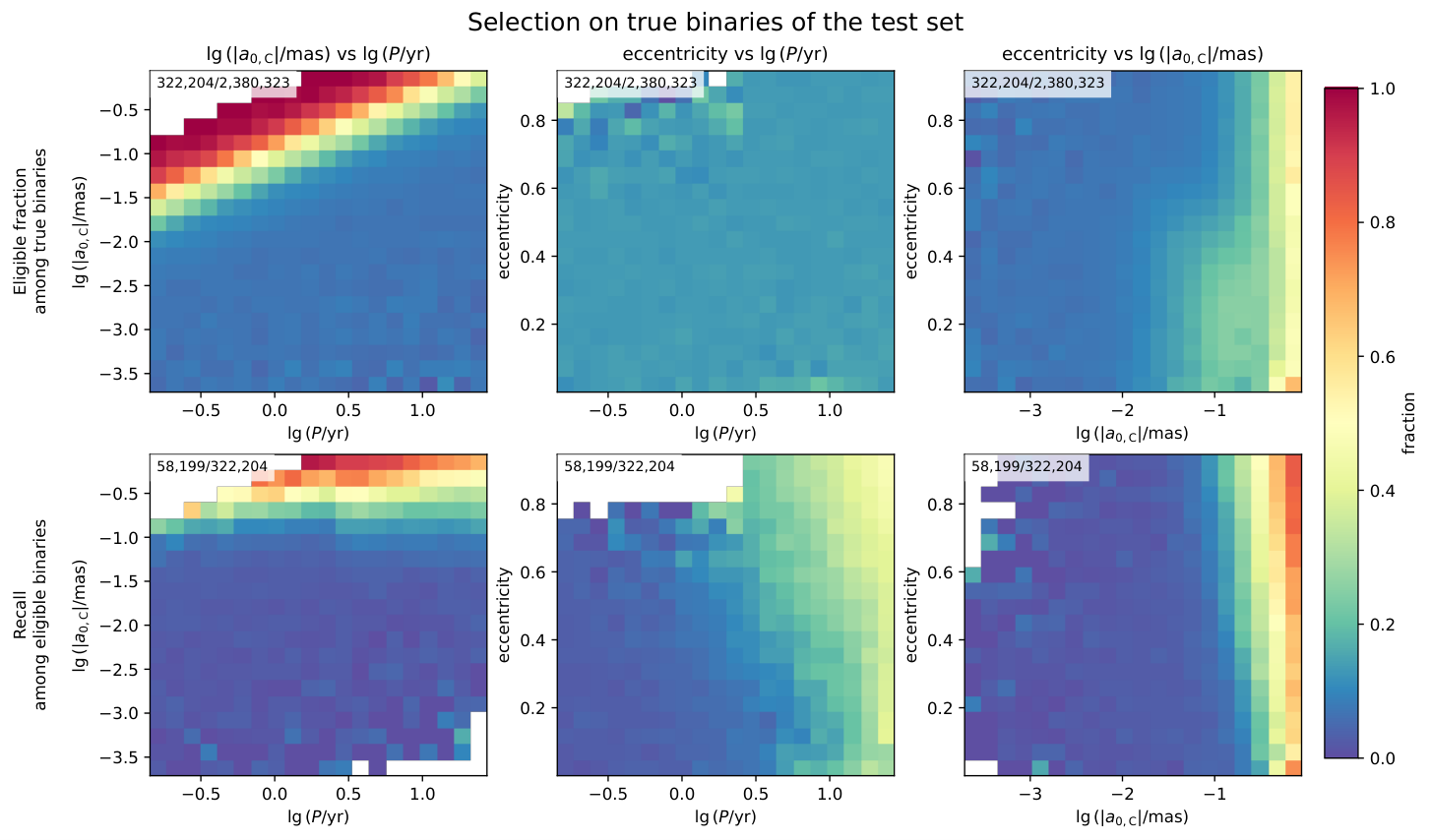
Fig. 3 shows the selection of true binaries in the test set. The top row shows the fraction of true binaries that are eligible for at least one stage, and the bottom row shows the recall among those eligible binaries. In each panel, the plotted range in each coordinate is set by the 0.5th and 99.5th percentiles of the corresponding distribution of true binaries in the test set. The numbers annotated in the upper-left corner of the panels give eligible/total true binaries in the test set in the first row and selected/eligible true binaries in the second row.

The dominant trend is with the photocentric semi-major axis. Binaries with larger values of the photocentric semi-major axis $|a_{0,\rm C}|$ ⁸⁸ 8 We use the CSST photocentric semi-major axis because $a_{0}$ is mission dependent through the passband-integrated flux ratio, and Gaia has no observations for sources fainter than $G\gtrsim 21$ . are both more likely to be eligible and more likely to be recalled once eligible for at least one stage. A period dependence is also visible. At fixed photocentric semi-major axis, the recall changes with orbital period because the 5p residuals, PMa, and observational coverage respond to different orbital periods. The eccentricity dependence is weaker but still visible. Higher eccentricity binaries produce faster photocenter motion near periastron. When the motion close to periastron is sampled, the 5p model absorbs the orbital motion less efficiently. This mainly increases the positional offset significances, which modestly improves the recall once the source is eligible for at least one stage.

6 Orbital solution results

6.1 Definition of selection tiers

We applied the 12p orbital fit to the candidates selected in Sect. 5.2. This sample contains $72\,554$ sources, of which $58\,199$ are true binaries and $14\,355$ are single stars. The fitting algorithm is described in Appx. .

We define two nested selection tiers for the fitted solutions. The 12p model preference tier requires

\displaystyle\Delta{\rm BIC}={\rm BIC}_{5\rm p}-{\rm BIC}_{12\rm p}\geq 10.

(15)

Here, BIC denotes the Bayesian information criterion, and the subscripts identify the 5p and 12p models. A positive $\Delta{\rm BIC}$ favors the 12p model, and the adopted threshold of 10 requires strong evidence for the 12p model (Liddle, 2007).

The fiducial tier is a more restrictive subset of the 12p model preference tier. It additionally requires $F_{2,12{\rm p}}<25$ , where $F_{2,12{\rm p}}$ is the $F_{2}$ statistic of the 12p solution, and $s_{a_{0}}=a_{0}/\sigma_{a_{0}}>1$ , where $s_{a_{0}}$ is the photocentric semi-major-axis significance. We also exclude solutions that converge at the upper eccentricity boundary $e=0.99$ (Hara et al., 2019).

6.2 Summary of the orbital solution

Table 4: Orbital solution results for the candidate sample ^{a
aa}^{a
aa}

a

The candidate sample contains

72\,554

sources, of which

58\,199

are true binaries and

14\,355

are single stars..⁹⁹ 9 Notes.

Scenario	12p-fitted sources^{b bb}^{b bb} $b$ A source is counted only if it satisfies the mock requirements for that scenario; the joint scenario additionally requires observations from both missions.	Selected sources (binary/single; percentage^{c cc}^{c cc} $c$ Each percentage uses the number of 12p-fitted true binaries in that row as its denominator.)
	binary/single	12p model preference	Fiducial
Gaia	$58\,147$ / $14\,282$	$7\,307$ / $0$ ; $12.57\%$	$3\,930$ / $0$ ; $6.76\%$
CSST	$6\,715$ / $2\,804$	$35$ / $0$ ; $0.52\%$	$12$ / $0$ ; $0.18\%$
Joint	$9\,403$ / $3\,241$	$2\,010$ / $0$ ; $21.38\%$	$984$ / $0$ ; $10.46\%$

Table a summarizes the two selection tiers for the 12p solutions. The 12p-fitted samples still contain single stars because the nonlinear 12p model can formally converge for single-star epoch data. In all three scenarios, none of the fitted simulated single stars satisfies the 12p model preference criterion $\Delta{\rm BIC}\geq 10$ . Within this simulation, the adopted $\Delta{\rm BIC}$ threshold therefore removes all single-star false positives that formally converge under the 12p model.

The numbers in the two selection tiers differ among the scenarios. The joint 12p-fitted sample is smaller than the Gaia 12p-fitted sample because it is drawn from the smaller subset of candidates that have observations from both missions and satisfy the joint effective observation requirement in Sect. 4.2. CSST alone yields only $35$ solutions in the 12p model preference tier and $12$ fiducial solutions. This small yield is consistent with the adopted CSST observing schedule. Although CSST provides high-precision astrometric measurements, the temporal sampling is often too uneven for 12p solutions to satisfy the fiducial criteria. The joint fit yields $2\,010$ 12p model preference and $984$ fiducial solutions, corresponding to $21.38\%$ and $10.46\%$ of the fitted true binaries. In the scenario-specific fitted samples, the joint solution raises the 12p model preference fraction from $12.57\%$ for the Gaia fit to $21.38\%$ for the joint fit, and the fiducial fraction from $6.76\%$ to $10.46\%$ .

The joint fit uses a single photocentric semi-major axis for both bands. We characterize the intrinsic shared- $a_{0}$ mismatch as $\Delta_{\rm shared}=\frac{1}{2}\left|a_{0,\rm C}-a_{0,\rm G}\right|$ , where $a_{0,\rm C}$ and $a_{0,\rm G}$ are the true photocentric semi-major axes for CSST and Gaia, respectively. For a common value adopted midway between the two band-specific true values, $\Delta_{\rm shared}$ is the absolute mismatch in each band; any other fitted $a_{0}$ produces a larger mismatch in one of the two bands. For the $984$ fiducial joint fits, $\Delta_{\rm shared}/|a_{0,\rm C}|$ has a median of $0.077$ and a 99th percentile of $0.106$ ; $\Delta_{\rm shared}/|a_{0,\rm G}|$ has a median of $0.091$ and a 99th percentile of $0.134$ . For these fiducial joint fits, the formal fractional $a_{0}$ uncertainty $\sigma_{a_{0}}/a_{0}$ has a median of $0.337$ . At the population level, the shared- $a_{0}$ mismatch is therefore smaller than the typical reported formal $a_{0}$ uncertainty in this simulation.

Figure 4: Histogram of the

\Delta{\rm BIC}

values for 12p-fitted sources. The panels show the Gaia, CSST, and joint solutions from left to right. Red and blue histograms represent binaries and single stars in the candidate set, respectively. The vertical dashed line marks

\Delta{\rm BIC}=10

, which defines the 12p model preference criterion. Only the range between the 0.1st and 99.9th percentiles of

\Delta{\rm BIC}

is shown.

Fig. 4 illustrates the 12p model preference criterion. In the Gaia and joint panels, binaries develop a positive- $\Delta{\rm BIC}$ tail, while all 12p-fitted single stars remain below the $\Delta{\rm BIC}=10$ threshold. The CSST panel shows much stronger overlap between the binary and single-star $\Delta{\rm BIC}$ distributions, and only a small number of sources pass the threshold. This explains the small number of CSST solutions in the 12p model preference tier, whereas the joint fit yields many more such solutions.

6.3 Properties of the selected 12p solution subsets

Fig. 5 compares the fitted and true orbital periods of 12p-fitted true binaries. The light grey background points show the 12p fits satisfying neither selection tier. Their broad distribution indicates that obtaining a converged 12p fit does not guarantee accurate recovery of the orbital period. In the Gaia and joint panels, the blue contours represent solutions that satisfy only the 12p model preference criterion, and the orange contours represent fiducial solutions. Both selected groups are more concentrated around $P_{\rm fit}=P_{\rm true}$ than the light-grey background points, and the fiducial solutions are more tightly concentrated than the solutions satisfying only the 12p model preference criterion. The two selected CSST groups contain too few solutions for stable density contours, so their sources are plotted individually.

Fig. 6 shows the 12p-fitted sources in the $\Delta{\rm BIC}$ – $s_{a_{0}}$ plane, where $s_{a_{0}}=a_{0}/\sigma_{a_{0}}$ . The uncertainty $\sigma_{a_{0}}$ is returned by the 12p orbital fit and therefore depends on the number of observations, observational distribution and precision. A large $\Delta{\rm BIC}$ selects fits for which the 12p model is preferred over the 5p model, but it does not establish accurate recovery of the orbital parameters. In the Gaia and joint panels, many orbital solutions satisfying only the 12p model preference criterion have $s_{a_{0}}\leq 1$ . The fiducial tier requires $s_{a_{0}}>1$ and therefore excludes these fits. The fiducial subset accounts for a larger fraction of the 12p-fitted true binaries in the joint scenario than in the Gaia scenario. Fig. 5 shows that the fiducial joint subset is more concentrated around $P_{\rm fit}=P_{\rm true}$ in this simulation.

Fig. 7 shows the fraction of 12p-fitted true binaries satisfying the fiducial criteria in bins of $P_{\rm true}$ and $P_{\rm true}/T_{\rm obs}$ , where $T_{\rm obs}$ is the time baseline for each source. At a fixed $P_{\rm true}$ , a shorter $T_{\rm obs}$ yields a larger $P_{\rm true}/T_{\rm obs}$ and a smaller observed orbital fraction. This ratio therefore measures the temporal coverage available for detecting the orbit and recovering its period.

In the left panel, the joint fiducial fraction is higher than the Gaia fraction toward the long-period end. At $P_{\rm true}<1\,{\rm yr}$ , the fiducial fractions decrease rapidly in the Gaia and joint scenarios. At fixed component masses, flux ratio, and parallax, shorter-period binaries have smaller photocentric semi-major axes and are therefore more difficult to detect. Gaia scan-angle-dependent signals can additionally introduce period aliases in this regime (Holl et al., 2023a). This behavior is consistent with Fig. 5, where fiducial solutions and solutions satisfying only the 12p model preference criterion are both rare at $P_{\rm true}<1\,{\rm yr}$ . In the right panel, the fiducial fractions for both the Gaia and joint solutions decrease once the true orbital period exceeds the observational time baseline. This pattern is consistent with temporal coverage contributing to the higher joint fiducial fraction at long periods. The CSST fiducial fraction remains low under the current survey schedule.

Figure 7: Fiducial fractions among 12p-fitted true binaries versus the true orbital period

P_{\rm true}

(left) and the ratio of the true orbital period to the observational time baseline of each source

P_{\rm true}/T_{\rm obs}

(right), for the Gaia, CSST, and joint solutions. In each bin, the numerator is the number of true binaries satisfying the fiducial criteria, and the denominator is the number of 12p-fitted true binaries in the same scenario and bin. The legend gives the total fiducial/12p-fitted counts for each scenario.

For binaries with $P_{\rm true}>15\,{\rm yr}$ , $482$ of $20\,330$ successfully fitted binaries in the Gaia scenario and $202$ of $2\,978$ in the joint scenario satisfy the fiducial criteria. These counts correspond to $2.37\%$ and $6.78\%$ , respectively. Joint fitting therefore raises the long-period fiducial fraction from $2.37\%$ to $6.78\%$ , a factor of $2.86$ , in the scenario-specific fitted samples.

Much of this gain comes from the longer time baseline. Among the scenario-specific long-period fitted samples, the median $T_{\rm obs}$ increases from $10.18\,{\rm yr}$ for Gaia to $17.27\,{\rm yr}$ for the joint scenario, while the median $P_{\rm true}/T_{\rm obs}$ decreases from $2.07$ to $1.20$ . The joint data therefore cover a larger fraction of these long-period orbits. Among all long-period fiducial solutions in each scenario, the median absolute relative period error, $|P_{\rm fit}-P_{\rm true}|/P_{\rm true}$ , is $40.7\%$ for Gaia and $11.1\%$ for the joint fit.

The fiducial tier requires $\Delta{\rm BIC}\geq 10$ , $F_{2,12{\rm p}}<25$ , and $s_{a_{0}}>1$ , and excludes solutions that converge at the upper eccentricity boundary $e=0.99$ . The CSST-only 12p results remain limited by the current survey schedule. Relative to the Gaia-only solution, the joint solution increases the 12p model preference and fiducial fractions from $12.57\%$ and $6.76\%$ to $21.38\%$ and $10.46\%$ in the scenario-specific samples, respectively. For the long-period fiducial subsets, the joint solutions have a smaller median absolute relative period error than the Gaia solutions.

7 Effect of the CSST cadence on 12p orbit fitting

CSST will reserve approximately 10% of its observing time for public proposals during the 10-year initial mission (CSST Collaboration et al., 2026). One use of this time is targeted follow-up of sources that are already known or strongly suspected to be binaries. Such observations can improve the binary orbital coverage by scheduling observations at more regular epochs. The number of 12p fits satisfying the selection criteria depends on observational precision, time baseline, and cadence regularity, motivating a test of how a more regular cadence changes this yield.

To isolate the effect of the observing schedule from the candidate-selection procedure, we randomly selected $500\,000$ binaries from the simulated catalog and did not include single stars in this test. This setup represents a sample of identified binary candidates with no orbital solutions, such as those selected from PMa or overluminosity, for which the main question is whether the epoch data can yield an orbital solution rather than whether the sources can first be distinguished from single stars. For each source and observing schedule, we generated mock observations and fitted both the 5p and 12p models. We then applied the same selection criteria as in Sect. 6.1.

We compared the current CSST survey schedule with three regular schedules. The current schedule is the CSST schedule described in Sect. 2.1. In the regular schedules, we kept the same CSST sky coverage but replaced the schedule with uniformly sampled epochs over the 10-year CSST baseline. We tested three schedules with $25$ , $50$ , and $100$ CSST observations, denoted U25, U50, and U100, respectively. The U25 schedule is the most direct comparison with the current schedule, because the current schedule provides $27.6$ CSST observations on average. Thus, U25 is approximately a redistribution of the current observations with a similar observational budget. For the joint solutions, each CSST schedule was combined with the same Gaia scanning law.

Fig. 8 compares the Gaia and joint solutions in the $G$ band. At $G<19$ , the Gaia fit yields $842$ fiducial solutions. The joint fit with the current CSST schedule yields $232$ , because it is restricted to sources with both Gaia and CSST observations. Replacing the current schedule with the U25 schedule increases the joint count from $232$ to $294$ fiducial solutions. The denser U50 and U100 schedules further increase the yield to $340$ and $400$ , respectively. At $19<G<21$ , the joint fiducial count increases from $4$ for the current schedule to $5$ , $7$ , and $19$ for U25, U50, and U100.

For CSST, the fiducial solutions are concentrated at the bright end. Within $17.8<g<19$ , the current schedule yields $2$ fiducial solutions. U25 increases this to $28$ solutions, while U50 and U100 further increase the yield to $43$ and $78$ , respectively. At $19<g<21$ , the corresponding counts for the current, U25, U50, and U100 schedules are $2$ , $6$ , $12$ , and $18$ . CSST fiducial solutions remain rare at $g>21$ for all schedules.

Comparing within the CSST $g$ -band, the joint fit yields more fiducial solutions than the CSST-only fit. At $17.8<g<19$ , the joint fit with the current CSST schedule yields $173$ fiducial solutions. U25 increases this number to $222$ , while U50 and U100 further increase it to $247$ and $288$ . At $19<g<21$ , the joint fiducial solution count increases from $61$ for the current schedule to $75$ , $98$ , and $127$ for U25, U50, and U100. At $g>21$ , even the joint fit yields very few fiducial solutions. The small number of joint solutions in this regime is expected because some sources with $G<21$ are included in the Gaia mock observations but have $g>21$ (see Fig. 1).

These results show that a more regular CSST cadence can increase the number of fits satisfying the fiducial criteria. U25 increases the yield while using nearly the same number of CSST observations as the current schedule. Additional observations in U50 and U100 continue to increase the yield, but the increase is concentrated in relatively bright sources with $g\lesssim 21$ . The simulated schedules suggest that proposed CSST observations, or adjustments to the survey schedule, could be used to reobserve bright binary candidates more regularly and provide better temporal sampling for subsequent orbit fitting.

8 Conclusion and discussion

We have presented an assessment of the detectability of unresolved binaries using mock observations for CSST, Gaia, and their joint epoch astrometry. We sampled the input catalog from MWMSC, which represents the underlying Galactic population, evolved binaries with COSMIC, calculated stellar parameters and Gaia photometry with isochrones, and constructed the CSST photometry using the adopted response curves, blackbody colors, and extinction in the CSST $g$ band.

The hierarchical candidate classifier identifies candidates for the computationally expensive 12p orbital fit. The classifier uses 5p diagnostics, PMa features, and auxiliary features based on observational cadence. On the independent test set, it selected $72\,554$ candidates among sources eligible for at least one stage, including $58\,199$ true binaries and $14\,355$ single stars. The resulting precision is $0.802$ , and the recall among eligible binaries is $0.181$ (Table 3). Candidate selection mainly depends on the photocentric semi-major axis and the orbital period, with only a weak dependence on eccentricity. This trend is consistent with larger photocentric orbits producing stronger 5p residuals, PMa, and related astrometric diagnostics.

In the candidate set, the 12p model preference criterion $\Delta{\rm BIC}\geq 10$ excludes all single stars with formally converged but spurious 12p fits in this simulation. Only a subset of the 12p fits satisfies the fiducial criteria. The fiducial tier requires $\Delta{\rm BIC}\geq 10$ , $F_{2,12{\rm p}}<25$ , $s_{a_{0}}>1$ , and no convergence at the upper eccentricity boundary $e=0.99$ . The Gaia fit yields $3\,930$ fiducial solutions, while the joint fit yields $984$ from its smaller fitted sample (Table a ). Relative to the Gaia-only fit, the joint fit increases the fraction of fitted binaries satisfying the 12p model preference criterion from $12.57\%$ to $21.38\%$ and the fiducial fraction from $6.76\%$ to $10.46\%$ in the scenario-specific samples.

Under the current survey schedule, few CSST 12p fits satisfy the fiducial criteria. In the candidate sample, CSST yields only $35$ solutions in the 12p model preference tier and $12$ in the fiducial tier. The current schedule often provides uneven temporal sampling and therefore incomplete orbital-phase coverage. This uneven sampling is associated with the low fiducial yield, despite CSST having single-epoch precision comparable to that of a Gaia FoV transit.

A separate single-stage classifier using only the CSST 5p diagnostics and CSST observational-sampling features was trained, tuned, and applied to the $124\,491$ CSST-eligible test sources, including $41\,302$ true binaries. The CSST classifier selected $1\,736$ candidates, comprising $1\,379$ true binaries and $357$ single stars, with a precision of $0.794$ and a recall of $0.0334$ . This low recall and the small CSST 12p yield are consistent with the limited orbital-phase coverage produced by the current uneven survey schedule.

The idealized cadence experiments motivate investigating operationally feasible ways to obtain more regular follow-up observations of bright binary candidates. Redistributing a comparable number of CSST observations ( $27.6$ on average) into a uniformly sampled 25-observation schedule (U25) increases both CSST and joint yields. U50 and U100 further increase the number of fits satisfying the fiducial criteria. The gain is concentrated at the bright end, primarily for sources with $g\lesssim 21$ . This result suggests that CSST public proposals or future schedule adjustments could target bright binary candidates with a more regular cadence for subsequent orbit fitting.

Several limitations remain. First, the adopted CSST single-epoch observation errors are predictions with an added attitude-noise term. The in-orbit single-epoch observation errors can only be measured after CSST has operated for a sufficient period. Second, the U25, U50, and U100 cases are idealized cadence experiments rather than operational schedule designs. They do not account for operational constraints such as target visibility windows, spacecraft attitude constraints, calibration requirements, or competition with other science proposals. Third, the joint 12p fit uses a single photocentric semi-major axis for both missions, whereas $a_{0,\rm G}$ and $a_{0,\rm C}$ are passband-dependent. At the population level, the mismatch associated with this approximation is smaller than the typical reported formal $a_{0}$ uncertainty for the fiducial joint fits in this simulation. Fourth, the simulation does not include photocenter variability induced by stellar activity, crowding, higher-order multiplicity, window truncation, or catalog calibration systematics. Finally, the population-level assessment in this work focuses on unresolved binaries. The resolved-binary toy experiment in Appx. shows a sharp decrease in the relative-error distribution between $a=70\,{\rm mas}$ and $a=80\,{\rm mas}$ . At $a=80\,{\rm mas}$ , all $100$ injected binaries return 13p (12p + mass ratio) solutions and $99$ satisfy the additional quality criteria. Across $90\leq a\leq 500\,{\rm mas}$ , all $4\,200$ injected binaries return solutions and $4\,199$ satisfy the criteria under the adopted 48-epoch sampling.

The main conclusion is that, in our simulation, joint CSST and Gaia epoch astrometry raises the fractions of fitted unresolved binaries satisfying the 12p model preference and fiducial criteria relative to the Gaia-only solution. For fitted true binaries with $P_{\rm true}>15\,{\rm yr}$ , joint fitting increases the fiducial fraction from $2.37\%$ to $6.78\%$ in the scenario-specific samples. The longer joint baseline covers a larger fraction of these orbits, and the joint long-period fiducial sample has a smaller median relative period error. Under the present wide-field schedule, CSST alone yields few fiducial 12p fits for unresolved binaries. Binary candidates can be selected using 5p diagnostics and astrometric anomaly features such as PMa. More regular CSST observations of binary candidates can then improve temporal coverage for subsequent 12p orbit fitting and application of the selection criteria. Within the overlapping magnitude range, joint CSST and Gaia epoch astrometry can also extend the search to binaries that are fainter than most sources in the Gaia non-single-star catalog while retaining sensitivity to longer periods. Such an expanded sample can provide additional dynamical mass measurements of compact companions and help test whether the observed neutron-star–black-hole mass gap traces the underlying compact-object population or observational selection.

Acknowledgements.

We sincerely thank the expert referee, Frédéric Arenou, for his careful, detailed, and insightful comments, which substantially improved the manuscript. This work was supported by the National Key R&D Program of China (Grant No. 2023YFA1607901), the Youth Innovation Promotion Association CAS, the grants from the Natural Science Foundation of Shanghai through grant 21ZR1474100, National Natural Science Foundation of China (NSFC) through grants 12173069, and the Talent Plan of Shanghai Branch, Chinese Academy of Sciences with No.CASSHB-QNPD-2023-016. We acknowledge the science research grants from the China Manned Space Project with NO.CMS-CSST-2021-A12 and NO.CMS-CSST-2021-B10. We thank Yang Chen and Yifan Xuan for their assistance in accessing the Milky Way stellar mock catalog. We are grateful to the editor, Thierry Forveille, for his constructive comment that helped to improve the manuscript. This work made use of data from the Gaia Observation Forecast Tool (https://gaia.esac.esa.int/gost/) and the High Performance Computing Resource in the Core Facility for Advanced Research Computing at Shanghai Astronomical Observatory. We thank the developers and contributors of the following software packages and tools: astropy (Astropy Collaboration et al., 2022), COSMIC (Breivik et al., 2020), healpy (Zonca et al., 2019), isochrones (Morton, 2015), jplephem (Rhodes, 2011), matplotlib (Hunter, 2007), numpy (Harris et al., 2020), optuna (Akiba et al., 2019), pandas (McKinney, 2010), TOPCAT (Taylor, 2005), scikit-learn (Pedregosa et al., 2011), and scipy (Virtanen et al., 2020).

References

Abreu et al. (2025) A. Abreu, J. Lillo-Box, A. M. Perez-Garcia, J. Sahlmann, J. H. J. de Bruijne, and C. Cifuentes ExoDNN: Boosting exoplanet detection with artificial intelligence: Application to Gaia Data Release 3. A&A 704, pp. A150. External Links: Document, 2602.02910, ADS entry Cited by: §5.1, §5.
Akiba et al. (2019) T. Akiba, S. Sano, T. Yanase, T. Ohta, and M. Koyama Optuna: A Next-generation Hyperparameter Optimization Framework. In Proceedings of the 25th ACM SIGKDD International Conference on Knowledge Discovery and Data Mining, pp. 2623–2631. External Links: Document Cited by: §8.
Astropy Collaboration et al. (2022) Astropy Collaboration, A. M. Price-Whelan, P. L. Lim, N. Earl, N. Starkman, L. Bradley, D. L. Shupe, A. A. Patil, L. Corrales, C. E. Brasseur, M. Nöthe, A. Donath, E. Tollerud, B. M. Morris, A. Ginsburg, E. Vaher, B. A. Weaver, J. Tocknell, W. Jamieson, M. H. van Kerkwijk, T. P. Robitaille, B. Merry, M. Bachetti, H. M. Günther, T. L. Aldcroft, J. A. Alvarado-Montes, A. M. Archibald, A. Bódi, S. Bapat, G. Barentsen, J. Bazán, M. Biswas, M. Boquien, D. J. Burke, D. Cara, M. Cara, K. E. Conroy, S. Conseil, M. W. Craig, R. M. Cross, K. L. Cruz, F. D’Eugenio, N. Dencheva, H. A. R. Devillepoix, J. P. Dietrich, A. D. Eigenbrot, T. Erben, L. Ferreira, D. Foreman-Mackey, R. Fox, N. Freij, S. Garg, R. Geda, L. Glattly, Y. Gondhalekar, K. D. Gordon, D. Grant, P. Greenfield, A. M. Groener, S. Guest, S. Gurovich, R. Handberg, A. Hart, Z. Hatfield-Dodds, D. Homeier, G. Hosseinzadeh, T. Jenness, C. K. Jones, P. Joseph, J. B. Kalmbach, E. Karamehmetoglu, M. Kałuszyński, M. S. P. Kelley, N. Kern, W. E. Kerzendorf, E. W. Koch, S. Kulumani, A. Lee, C. Ly, Z. Ma, C. MacBride, J. M. Maljaars, D. Muna, N. A. Murphy, H. Norman, R. O’Steen, K. A. Oman, C. Pacifici, S. Pascual, J. Pascual-Granado, R. R. Patil, G. I. Perren, T. E. Pickering, T. Rastogi, B. R. Roulston, D. F. Ryan, E. S. Rykoff, J. Sabater, P. Sakurikar, J. Salgado, A. Sanghi, N. Saunders, V. Savchenko, L. Schwardt, M. Seifert-Eckert, A. Y. Shih, A. S. Jain, G. Shukla, J. Sick, C. Simpson, S. Singanamalla, L. P. Singer, J. Singhal, M. Sinha, B. M. Sipőcz, L. R. Spitler, D. Stansby, O. Streicher, J. Šumak, J. D. Swinbank, D. S. Taranu, N. Tewary, G. R. Tremblay, M. de Val-Borro, S. J. Van Kooten, Z. Vasović, S. Verma, J. V. de Miranda Cardoso, P. K. G. Williams, T. J. Wilson, B. Winkel, W. M. Wood-Vasey, R. Xue, P. Yoachim, C. Zhang, A. Zonca, and Astropy Project Contributors The Astropy Project: Sustaining and Growing a Community-oriented Open-source Project and the Latest Major Release (v5.0) of the Core Package. ApJ 935 (2), pp. 167. External Links: Document, 2206.14220, ADS entry Cited by: §8.
Brandt (2021) T. D. Brandt The Hipparcos-Gaia Catalog of Accelerations: Gaia EDR3 Edition. ApJS 254 (2), pp. 42. External Links: Document, 2105.11662, ADS entry Cited by: §5.1.2.
Breivik et al. (2020) K. Breivik, S. Coughlin, M. Zevin, C. L. Rodriguez, K. Kremer, C. S. Ye, J. J. Andrews, M. Kurkowski, M. C. Digman, S. L. Larson, and F. A. Rasio COSMIC Variance in Binary Population Synthesis. ApJ 898 (1), pp. 71. External Links: Document, 1911.00903, ADS entry Cited by: §3.1, §3.2, §8.
Castro-Ginard et al. (2024) A. Castro-Ginard, Z. Penoyre, A. R. Casey, A. G. A. Brown, V. Belokurov, T. Cantat-Gaudin, R. Drimmel, M. Fouesneau, S. Khanna, E. P. Kurbatov, A. M. Price-Whelan, H. Rix, and R. L. Smart Gaia DR3 detectability of unresolved binary systems. A&A 688, pp. A1. External Links: Document, 2404.14127, ADS entry Cited by: §1, §1, §5.1.3.
Chambers et al. (2016) K. C. Chambers, E. A. Magnier, N. Metcalfe, H. A. Flewelling, M. E. Huber, C. Z. Waters, L. Denneau, P. W. Draper, D. Farrow, D. P. Finkbeiner, C. Holmberg, J. Koppenhoefer, P. A. Price, A. Rest, R. P. Saglia, E. F. Schlafly, S. J. Smartt, W. Sweeney, R. J. Wainscoat, W. S. Burgett, S. Chastel, T. Grav, J. N. Heasley, K. W. Hodapp, R. Jedicke, N. Kaiser, R.-P. Kudritzki, G. A. Luppino, R. H. Lupton, D. G. Monet, J. S. Morgan, P. M. Onaka, B. Shiao, C. W. Stubbs, J. L. Tonry, R. White, E. Bañados, E. F. Bell, R. Bender, E. J. Bernard, M. Boegner, F. Boffi, M. T. Botticella, A. Calamida, S. Casertano, W.-P. Chen, X. Chen, S. Cole, N. Deacon, C. Frenk, A. Fitzsimmons, S. Gezari, V. Gibbs, C. Goessl, T. Goggia, R. Gourgue, B. Goldman, P. Grant, E. K. Grebel, N. C. Hambly, G. Hasinger, A. F. Heavens, T. M. Heckman, R. Henderson, T. Henning, M. Holman, U. Hopp, W.-H. Ip, S. Isani, M. Jackson, C. D. Keyes, A. M. Koekemoer, R. Kotak, D. Le, D. Liska, K. S. Long, J. R. Lucey, M. Liu, N. F. Martin, G. Masci, B. McLean, E. Mindel, P. Misra, E. Morganson, D. N. A. Murphy, A. Obaika, G. Narayan, M. A. Nieto-Santisteban, P. Norberg, J. A. Peacock, E. A. Pier, M. Postman, N. Primak, C. Rae, A. Rai, A. Riess, A. Riffeser, H. W. Rix, S. Röser, R. Russel, L. Rutz, E. Schilbach, A. S. B. Schultz, D. Scolnic, L. Strolger, A. Szalay, S. Seitz, E. Small, K. W. Smith, D. R. Soderblom, P. Taylor, R. Thomson, A. N. Taylor, A. R. Thakar, J. Thiel, D. Thilker, D. Unger, Y. Urata, J. Valenti, J. Wagner, T. Walder, F. Walter, S. P. Watters, S. Werner, W. M. Wood-Vasey, and R. Wyse The Pan-STARRS1 Surveys. arXiv e-prints, pp. arXiv:1612.05560. External Links: Document, 1612.05560, ADS entry Cited by: §1, §3.1.
Chen et al. (2023) Y. Chen, X. Fu, C. Liu, P. Dal Tio, L. Girardi, G. Pastorelli, A. Mazzi, M. Trabucchi, H. Tian, D. Fan, P. Marigo, and A. Bressan The First Comprehensive Milky Way Stellar Mock Catalogue for the Chinese Space Station Telescope Survey Camera. Science China Physics, Mechanics and Astronomy 66 (11), pp. 119511. External Links: Document Cited by: §2.3, §3.1.
Choi et al. (2016) J. Choi, A. Dotter, C. Conroy, M. Cantiello, B. Paxton, and B. D. Johnson Mesa Isochrones and Stellar Tracks (MIST). I. Solar-scaled Models. ApJ 823 (2), pp. 102. External Links: Document, 1604.08592, ADS entry Cited by: §3.3.
Corral-Santana et al. (2016) J. M. Corral-Santana, J. Casares, T. Muñoz-Darias, F. E. Bauer, I. G. Martínez-Pais, and D. M. Russell BlackCAT: A catalogue of stellar-mass black holes in X-ray transients. Astronomy & Astrophysics 587, pp. A61. External Links: Document, 1510.08869, ADS entry Cited by: §1.
CSST Collaboration et al. (2026) CSST Collaboration, Y. Gong, H. Miao, H. Zhan, Z. Li, J. Shangguan, H. Li, C. Liu, X. Chen, H. Yuan, J. Zhou, H. Liu, C. Yu, J. Ji, Z. Qi, J. Liu, Z. Dai, X. Wang, Z. Zheng, L. Hao, J. Dou, Y. Ao, Z. Lin, K. Zhang, W. Wang, G. Sun, R. Li, G. Li, Y. Xu, X. Li, S. Li, P. Wu, J. Zhang, B. Wang, J. Bai, Y. Cai, Z. Cai, J. Cao, K. C. Chan, J. Chang, X. Chen, X. Chen, Y. Chen, Y. Chen, W. Cui, S. Dong, P. Du, W. Duan, J. Fan, L. Fan, Z. Fan, Z. Fan, T. Fang, J. Fu, L. Fu, Z. Fu, J. Gao, S. Gu, Y. Gu, Q. Guo, Z. Han, B. Hu, Z. Huang, L. C. Ho, L. Jiang, N. Jiang, Y. Jing, X. Kang, X. Kong, C. Li, C. Li, D. Li, J. Li, N. Li, Y. A. Li, S. Liao, W. Lin, F. Liu, J. Liu, X. Liu, Z. Liu, R. Mao, S. Mao, X. Meng, X. Pang, X. Peng, Y. Peng, H. Shan, J. Shen, S. Shen, Z. Shen, S. Shi, Y. Shi, S. Tan, H. Tian, J. Wang, J. Wang, X. Wang, Y. Wang, H. Wu, J. Wu, X. Wu, C. Xu, X. Xue, Y. Xue, J. Yang, X. Yang, Q. Yao, F. Yuan, Z. Yuan, J. Zhang, P. Zhang, T. Zhang, W. Zhang, X. Zhang, G. Zhao, G. Zhao, H. Zhong, J. Zhong, L. Zhou, W. Zhu, and Y. Zu Introduction to the Chinese Space Station Survey Telescope (CSST). Science China Physics, Mechanics, and Astronomy 69 (3), pp. 239501. External Links: Document, 2507.04618, ADS entry Cited by: Table 1, Table 1, §1, §2.1, §3.3, §3.3, §7, footnote 7.
Dey et al. (2019) A. Dey, D. J. Schlegel, D. Lang, R. Blum, K. Burleigh, X. Fan, J. R. Findlay, D. Finkbeiner, D. Herrera, S. Juneau, M. Landriau, M. Levi, I. McGreer, A. Meisner, A. D. Myers, J. Moustakas, P. Nugent, A. Patej, E. F. Schlafly, A. R. Walker, F. Valdes, B. A. Weaver, C. Yèche, H. Zou, X. Zhou, B. Abareshi, T. M. C. Abbott, B. Abolfathi, C. Aguilera, S. Alam, L. Allen, A. Alvarez, J. Annis, B. Ansarinejad, M. Aubert, J. Beechert, E. F. Bell, S. Y. BenZvi, F. Beutler, R. M. Bielby, A. S. Bolton, C. Briceño, E. J. Buckley-Geer, K. Butler, A. Calamida, R. G. Carlberg, P. Carter, R. Casas, F. J. Castander, Y. Choi, J. Comparat, E. Cukanovaite, T. Delubac, K. DeVries, S. Dey, G. Dhungana, M. Dickinson, Z. Ding, J. B. Donaldson, Y. Duan, C. J. Duckworth, S. Eftekharzadeh, D. J. Eisenstein, T. Etourneau, P. A. Fagrelius, J. Farihi, M. Fitzpatrick, A. Font-Ribera, L. Fulmer, B. T. Gänsicke, E. Gaztanaga, K. George, D. W. Gerdes, S. G. A. Gontcho, C. Gorgoni, G. Green, J. Guy, D. Harmer, M. Hernandez, K. Honscheid, L. W. Huang, D. J. James, B. T. Jannuzi, L. Jiang, R. Joyce, A. Karcher, S. Karkar, R. Kehoe, J. Kneib, A. Kueter-Young, T. Lan, T. R. Lauer, L. Le Guillou, A. Le Van Suu, J. H. Lee, M. Lesser, L. Perreault Levasseur, T. S. Li, J. L. Mann, R. Marshall, C. E. Martínez-Vázquez, P. Martini, H. du Mas des Bourboux, S. McManus, T. G. Meier, B. Ménard, N. Metcalfe, A. Muñoz-Gutiérrez, J. Najita, K. Napier, G. Narayan, J. A. Newman, J. Nie, B. Nord, D. J. Norman, K. A. G. Olsen, A. Paat, N. Palanque-Delabrouille, X. Peng, C. L. Poppett, M. R. Poremba, A. Prakash, D. Rabinowitz, A. Raichoor, M. Rezaie, A. N. Robertson, N. A. Roe, A. J. Ross, N. P. Ross, G. Rudnick, S. Safonova, A. Saha, F. J. Sánchez, E. Savary, H. Schweiker, A. Scott, H. Seo, H. Shan, D. R. Silva, Z. Slepian, C. Soto, D. Sprayberry, R. Staten, C. M. Stillman, R. J. Stupak, D. L. Summers, S. Sien Tie, H. Tirado, M. Vargas-Magaña, A. K. Vivas, R. H. Wechsler, D. Williams, J. Yang, Q. Yang, T. Yapici, D. Zaritsky, A. Zenteno, K. Zhang, T. Zhang, R. Zhou, and Z. Zhou Overview of the DESI Legacy Imaging Surveys. AJ 157 (5), pp. 168. External Links: Document, 1804.08657, ADS entry Cited by: §3.1.
Ding et al. (2025) Y. Ding, S. Liao, S. Wen, and Z. Qi Analysis of the Gaia Data Release 3 Parallax Bias at Bright Magnitudes. AJ 169 (4), pp. 211. External Links: Document, 2502.08068, ADS entry Cited by: §1.
Ding et al. (2024) Y. Ding, S. Liao, Q. Wu, Z. Qi, and Z. Tang Analysis of the Gaia Data Release 3 parallax bias in the Galactic plane. A&A 691, pp. A81. External Links: Document, 2409.15694, ADS entry Cited by: §1.
Dotter (2016) A. Dotter MESA Isochrones and Stellar Tracks (MIST) 0: Methods for the Construction of Stellar Isochrones. ApJS 222 (1), pp. 8. External Links: Document, 1601.05144, ADS entry Cited by: §3.3.
Duchêne and Kraus (2013) G. Duchêne and A. Kraus Stellar Multiplicity. ARA&A 51 (1), pp. 269–310. External Links: Document, 1303.3028, ADS entry Cited by: §1.
Duquennoy and Mayor (1991) A. Duquennoy and M. Mayor Multiplicity among Solar Type Stars in the Solar Neighbourhood - Part Two - Distribution of the Orbital Elements in an Unbiased Sample. A&A 248, pp. 485. External Links: ADS entry Cited by: §3.2.
El-Badry et al. (2024) K. El-Badry, C. Lam, B. Holl, J. Halbwachs, H. Rix, T. Mazeh, and S. Shahaf A generative model for Gaia astrometric orbit catalogs: selection functions for binary stars, giant planets, and compact object companions. The Open Journal of Astrophysics 7, pp. 100. External Links: Document, 2411.00088, ADS entry Cited by: Appendix A, Appendix A, §1, §1, §2.2, §3.3, §3.3, §4.1, §4.2, §4.2.
El-Badry et al. (2021) K. El-Badry, H. Rix, and T. M. Heintz A million binaries from Gaia eDR3: sample selection and validation of Gaia parallax uncertainties. MNRAS 506 (2), pp. 2269–2295. External Links: Document, 2101.05282, ADS entry Cited by: §1.
Euclid Collaboration et al. (2022) Euclid Collaboration, R. Scaramella, J. Amiaux, Y. Mellier, C. Burigana, C. S. Carvalho, J. -C. Cuillandre, A. Da Silva, A. Derosa, J. Dinis, E. Maiorano, M. Maris, I. Tereno, R. Laureijs, T. Boenke, G. Buenadicha, X. Dupac, L. M. Gaspar Venancio, P. Gómez-Álvarez, J. Hoar, J. Lorenzo Alvarez, G. D. Racca, G. Saavedra-Criado, J. Schwartz, R. Vavrek, M. Schirmer, H. Aussel, R. Azzollini, V. F. Cardone, M. Cropper, A. Ealet, B. Garilli, W. Gillard, B. R. Granett, L. Guzzo, H. Hoekstra, K. Jahnke, T. Kitching, T. Maciaszek, M. Meneghetti, L. Miller, R. Nakajima, S. M. Niemi, F. Pasian, W. J. Percival, S. Pottinger, M. Sauvage, M. Scodeggio, S. Wachter, A. Zacchei, N. Aghanim, A. Amara, T. Auphan, N. Auricchio, S. Awan, A. Balestra, R. Bender, C. Bodendorf, D. Bonino, E. Branchini, S. Brau-Nogue, M. Brescia, G. P. Candini, V. Capobianco, C. Carbone, R. G. Carlberg, J. Carretero, R. Casas, F. J. Castander, M. Castellano, S. Cavuoti, A. Cimatti, R. Cledassou, G. Congedo, C. J. Conselice, L. Conversi, Y. Copin, L. Corcione, A. Costille, F. Courbin, H. Degaudenzi, M. Douspis, F. Dubath, C. A. J. Duncan, S. Dusini, S. Farrens, S. Ferriol, P. Fosalba, N. Fourmanoit, M. Frailis, E. Franceschi, P. Franzetti, M. Fumana, B. Gillis, C. Giocoli, A. Grazian, F. Grupp, S. V. H. Haugan, W. Holmes, F. Hormuth, P. Hudelot, S. Kermiche, A. Kiessling, M. Kilbinger, R. Kohley, B. Kubik, M. Kümmel, M. Kunz, H. Kurki-Suonio, O. Lahav, S. Ligori, P. B. Lilje, I. Lloro, O. Mansutti, O. Marggraf, K. Markovic, F. Marulli, R. Massey, S. Maurogordato, M. Melchior, E. Merlin, G. Meylan, J. J. Mohr, M. Moresco, B. Morin, L. Moscardini, E. Munari, R. C. Nichol, C. Padilla, S. Paltani, J. Peacock, K. Pedersen, V. Pettorino, S. Pires, M. Poncet, L. Popa, L. Pozzetti, F. Raison, R. Rebolo, J. Rhodes, H. -W. Rix, M. Roncarelli, E. Rossetti, R. Saglia, P. Schneider, T. Schrabback, A. Secroun, G. Seidel, S. Serrano, C. Sirignano, G. Sirri, J. Skottfelt, L. Stanco, J. L. Starck, P. Tallada-Crespí, D. Tavagnacco, A. N. Taylor, H. I. Teplitz, R. Toledo-Moreo, F. Torradeflot, M. Trifoglio, E. A. Valentijn, L. Valenziano, G. A. Verdoes Kleijn, Y. Wang, N. Welikala, J. Weller, M. Wetzstein, G. Zamorani, J. Zoubian, S. Andreon, M. Baldi, S. Bardelli, A. Boucaud, S. Camera, D. Di Ferdinando, G. Fabbian, R. Farinelli, S. Galeotta, J. Graciá-Carpio, D. Maino, E. Medinaceli, S. Mei, C. Neissner, G. Polenta, A. Renzi, E. Romelli, C. Rosset, F. Sureau, M. Tenti, T. Vassallo, E. Zucca, C. Baccigalupi, A. Balaguera-Antolínez, P. Battaglia, A. Biviano, S. Borgani, E. Bozzo, R. Cabanac, and A. Cappi Euclid preparation. I. The Euclid Wide Survey. A&A 662, pp. A112. External Links: Document, 2108.01201, ADS entry Cited by: §1.
Figer (2005) D. F. Figer An upper limit to the masses of stars. Nature 434 (7030), pp. 192–194. External Links: Document, astro-ph/0503193, ADS entry Cited by: §3.1.
Fu et al. (2023) Z. Fu, Z. Qi, S. Liao, X. Peng, Y. Yu, Q. Wu, L. Shao, and Y. Xu Simulation of CSST’s astrometric capability. Frontiers in Astronomy and Space Sciences 10, pp. 1146603. External Links: Document, 2304.02196, ADS entry Cited by: Appendix A, §2.1, §2.1.
Gaia Collaboration et al. (2023) Gaia Collaboration, A. Vallenari, A. G. A. Brown, T. Prusti, J. H. J. de Bruijne, F. Arenou, C. Babusiaux, M. Biermann, O. L. Creevey, C. Ducourant, D. W. Evans, L. Eyer, R. Guerra, A. Hutton, C. Jordi, S. A. Klioner, U. L. Lammers, L. Lindegren, X. Luri, F. Mignard, C. Panem, D. Pourbaix, S. Randich, P. Sartoretti, C. Soubiran, P. Tanga, N. A. Walton, C. A. L. Bailer-Jones, U. Bastian, R. Drimmel, F. Jansen, D. Katz, M. G. Lattanzi, F. van Leeuwen, J. Bakker, C. Cacciari, J. Castañeda, F. De Angeli, C. Fabricius, M. Fouesneau, Y. Frémat, L. Galluccio, A. Guerrier, U. Heiter, E. Masana, R. Messineo, N. Mowlavi, C. Nicolas, K. Nienartowicz, F. Pailler, P. Panuzzo, F. Riclet, W. Roux, G. M. Seabroke, R. Sordo, F. Thévenin, G. Gracia-Abril, J. Portell, D. Teyssier, M. Altmann, R. Andrae, M. Audard, I. Bellas-Velidis, K. Benson, J. Berthier, R. Blomme, P. W. Burgess, D. Busonero, G. Busso, H. Cánovas, B. Carry, A. Cellino, N. Cheek, G. Clementini, Y. Damerdji, M. Davidson, P. de Teodoro, M. Nuñez Campos, L. Delchambre, A. Dell’Oro, P. Esquej, J. Fernández-Hernández, E. Fraile, D. Garabato, P. García-Lario, E. Gosset, R. Haigron, J. -L. Halbwachs, N. C. Hambly, D. L. Harrison, J. Hernández, D. Hestroffer, S. T. Hodgkin, B. Holl, K. Janßen, G. Jevardat de Fombelle, S. Jordan, A. Krone-Martins, A. C. Lanzafame, W. Löffler, O. Marchal, P. M. Marrese, A. Moitinho, K. Muinonen, P. Osborne, E. Pancino, T. Pauwels, A. Recio-Blanco, C. Reylé, M. Riello, L. Rimoldini, T. Roegiers, J. Rybizki, L. M. Sarro, C. Siopis, M. Smith, A. Sozzetti, E. Utrilla, M. van Leeuwen, U. Abbas, P. Ábrahám, A. Abreu Aramburu, C. Aerts, J. J. Aguado, M. Ajaj, F. Aldea-Montero, G. Altavilla, M. A. Álvarez, J. Alves, F. Anders, R. I. Anderson, E. Anglada Varela, T. Antoja, D. Baines, S. G. Baker, L. Balaguer-Núñez, E. Balbinot, Z. Balog, C. Barache, D. Barbato, M. Barros, M. A. Barstow, S. Bartolomé, J. -L. Bassilana, N. Bauchet, U. Becciani, M. Bellazzini, A. Berihuete, M. Bernet, S. Bertone, L. Bianchi, A. Binnenfeld, S. Blanco-Cuaresma, A. Blazere, T. Boch, A. Bombrun, D. Bossini, S. Bouquillon, A. Bragaglia, L. Bramante, E. Breedt, A. Bressan, N. Brouillet, E. Brugaletta, B. Bucciarelli, A. Burlacu, A. G. Butkevich, R. Buzzi, E. Caffau, R. Cancelliere, T. Cantat-Gaudin, R. Carballo, T. Carlucci, M. I. Carnerero, J. M. Carrasco, L. Casamiquela, M. Castellani, A. Castro-Ginard, L. Chaoul, P. Charlot, L. Chemin, V. Chiaramida, A. Chiavassa, N. Chornay, G. Comoretto, G. Contursi, W. J. Cooper, T. Cornez, S. Cowell, F. Crifo, M. Cropper, M. Crosta, C. Crowley, C. Dafonte, A. Dapergolas, M. David, P. David, P. de Laverny, F. De Luise, and R. De March Gaia Data Release 3. Summary of the content and survey properties. A&A 674, pp. A1. External Links: Document, 2208.00211, ADS entry Cited by: §1, §3.1.
Gandhi et al. (2022) P. Gandhi, D. A. H. Buckley, P. A. Charles, S. Hodgkin, S. Scaringi, C. Knigge, A. Rao, J. A. Paice, and Y. Zhao Astrometric excess noise in Gaia EDR3 and the search for X-ray binaries. MNRAS 510 (3), pp. 3885–3895. External Links: Document, 2201.00833, ADS entry Cited by: §5.1.1, §5.
Gentile Fusillo et al. (2019) N. P. Gentile Fusillo, P. Tremblay, B. T. Gänsicke, C. J. Manser, T. Cunningham, E. Cukanovaite, M. Hollands, T. Marsh, R. Raddi, S. Jordan, S. Toonen, S. Geier, M. Barstow, and J. D. Cummings A Gaia Data Release 2 catalogue of white dwarfs and a comparison with SDSS. MNRAS 482 (4), pp. 4570–4591. External Links: Document, 1807.03315, ADS entry Cited by: §2.3.
Girardi et al. (2005) L. Girardi, M. A. T. Groenewegen, E. Hatziminaoglou, and L. da Costa Star counts in the Galaxy. Simulating from very deep to very shallow photometric surveys with the TRILEGAL code. A&A 436 (3), pp. 895–915. External Links: Document, astro-ph/0504047, ADS entry Cited by: §3.1.
Girardi (2016) L. Girardi Milky Way populations with TRILEGAL. Astronomische Nachrichten 337 (8-9), pp. 871. External Links: Document, ADS entry Cited by: §3.1.
Gontcharov and Kiyaeva (2002) G. A. Gontcharov and O. V. Kiyaeva Photocentric orbits from a direct combination of ground-based astrometry with Hipparcos. I. Comparison with known orbits. A&A 391, pp. 647–657. External Links: Document, ADS entry Cited by: §3.3, §3.3.
Halbwachs et al. (2023) J. Halbwachs, D. Pourbaix, F. Arenou, L. Galluccio, P. Guillout, N. Bauchet, O. Marchal, G. Sadowski, and D. Teyssier Gaia Data Release 3. Astrometric binary star processing. A&A 674, pp. A9. External Links: Document, 2206.05726, ADS entry Cited by: Appendix A, §1, §5.1.1.
Hara et al. (2019) N. C. Hara, G. Boué, J. Laskar, J.-B. Delisle, and N. Unger Bias and robustness of eccentricity estimates from radial velocity data. MNRAS 489 (1), pp. 738–762. External Links: Document, 1907.02048, ADS entry Cited by: §6.1.
Harris et al. (2020) C. R. Harris, K. J. Millman, S. J. van der Walt, R. Gommers, P. Virtanen, D. Cournapeau, E. Wieser, J. Taylor, S. Berg, N. J. Smith, R. Kern, M. Picus, S. Hoyer, M. H. van Kerkwijk, M. Brett, A. Haldane, J. F. del Río, M. Wiebe, P. Peterson, P. Gérard-Marchant, K. Sheppard, T. Reddy, W. Weckesser, H. Abbasi, C. Gohlke, and T. E. Oliphant Array programming with NumPy. Nature 585 (7825), pp. 357–362. External Links: Document, Link Cited by: §8.
Holl et al. (2023a) B. Holl, C. Fabricius, J. Portell, L. Lindegren, P. Panuzzo, M. Bernet, J. Castañeda, G. Jevardat de Fombelle, M. Audard, C. Ducourant, D. L. Harrison, D. W. Evans, G. Busso, A. Sozzetti, E. Gosset, F. Arenou, F. De Angeli, M. Riello, L. Eyer, L. Rimoldini, P. Gavras, N. Mowlavi, K. Nienartowicz, I. Lecoeur-Taïbi, P. García-Lario, and D. Pourbaix Gaia Data Release 3. Gaia scan-angle-dependent signals and spurious periods. A&A 674, pp. A25. External Links: Document, 2212.11971, ADS entry Cited by: Appendix A, §3.3, §6.3.
Holl et al. (2023b) B. Holl, A. Sozzetti, J. Sahlmann, P. Giacobbe, D. Ségransan, N. Unger, J. -B. Delisle, D. Barbato, M. G. Lattanzi, R. Morbidelli, and D. Sosnowska Gaia Data Release 3. Astrometric orbit determination with Markov chain Monte Carlo and genetic algorithms: Systems with stellar, sub-stellar, and planetary mass companions. A&A 674, pp. A10. External Links: Document, 2206.05439, ADS entry Cited by: §5.1.1.
Hunter (2007) J. D. Hunter Matplotlib: A 2D Graphics Environment. Computing in Science and Engineering 9 (3), pp. 90–95. External Links: Document, ADS entry Cited by: §8.
Ivezić et al. (2019) Ž. Ivezić, S. M. Kahn, J. A. Tyson, B. Abel, E. Acosta, R. Allsman, D. Alonso, Y. AlSayyad, S. F. Anderson, J. Andrew, J. R. P. Angel, G. Z. Angeli, R. Ansari, P. Antilogus, C. Araujo, R. Armstrong, K. T. Arndt, P. Astier, É. Aubourg, N. Auza, T. S. Axelrod, D. J. Bard, J. D. Barr, A. Barrau, J. G. Bartlett, A. E. Bauer, B. J. Bauman, S. Baumont, E. Bechtol, K. Bechtol, A. C. Becker, J. Becla, C. Beldica, S. Bellavia, F. B. Bianco, R. Biswas, G. Blanc, J. Blazek, R. D. Blandford, J. S. Bloom, J. Bogart, T. W. Bond, M. T. Booth, A. W. Borgland, K. Borne, J. F. Bosch, D. Boutigny, C. A. Brackett, A. Bradshaw, W. N. Brandt, M. E. Brown, J. S. Bullock, P. Burchat, D. L. Burke, G. Cagnoli, D. Calabrese, S. Callahan, A. L. Callen, J. L. Carlin, E. L. Carlson, S. Chandrasekharan, G. Charles-Emerson, S. Chesley, E. C. Cheu, H. Chiang, J. Chiang, C. Chirino, D. Chow, D. R. Ciardi, C. F. Claver, J. Cohen-Tanugi, J. J. Cockrum, R. Coles, A. J. Connolly, K. H. Cook, A. Cooray, K. R. Covey, C. Cribbs, W. Cui, R. Cutri, P. N. Daly, S. F. Daniel, F. Daruich, G. Daubard, G. Daues, W. Dawson, F. Delgado, A. Dellapenna, R. de Peyster, M. de Val-Borro, S. W. Digel, P. Doherty, R. Dubois, G. P. Dubois-Felsmann, J. Durech, F. Economou, T. Eifler, M. Eracleous, B. L. Emmons, A. Fausti Neto, H. Ferguson, E. Figueroa, M. Fisher-Levine, W. Focke, M. D. Foss, J. Frank, M. D. Freemon, E. Gangler, E. Gawiser, J. C. Geary, P. Gee, M. Geha, C. J. B. Gessner, R. R. Gibson, D. K. Gilmore, T. Glanzman, W. Glick, T. Goldina, D. A. Goldstein, I. Goodenow, M. L. Graham, W. J. Gressler, P. Gris, L. P. Guy, A. Guyonnet, G. Haller, R. Harris, P. A. Hascall, J. Haupt, F. Hernandez, S. Herrmann, E. Hileman, J. Hoblitt, J. A. Hodgson, C. Hogan, J. D. Howard, D. Huang, M. E. Huffer, P. Ingraham, W. R. Innes, S. H. Jacoby, B. Jain, F. Jammes, M. J. Jee, T. Jenness, G. Jernigan, D. Jevremović, K. Johns, A. S. Johnson, M. W. G. Johnson, R. L. Jones, C. Juramy-Gilles, M. Jurić, J. S. Kalirai, N. J. Kallivayalil, B. Kalmbach, J. P. Kantor, P. Karst, M. M. Kasliwal, H. Kelly, R. Kessler, V. Kinnison, D. Kirkby, L. Knox, I. V. Kotov, V. L. Krabbendam, K. S. Krughoff, P. Kubánek, J. Kuczewski, S. Kulkarni, J. Ku, N. R. Kurita, C. S. Lage, R. Lambert, T. Lange, J. B. Langton, L. Le Guillou, D. Levine, M. Liang, K. Lim, C. J. Lintott, K. E. Long, M. Lopez, P. J. Lotz, R. H. Lupton, N. B. Lust, L. A. MacArthur, A. Mahabal, R. Mandelbaum, T. W. Markiewicz, D. S. Marsh, P. J. Marshall, S. Marshall, M. May, R. McKercher, M. McQueen, J. Meyers, M. Migliore, M. Miller, and D. J. Mills LSST: From Science Drivers to Reference Design and Anticipated Data Products. ApJ 873 (2), pp. 111. External Links: Document, 0805.2366, ADS entry Cited by: §1.
Kervella et al. (2019) P. Kervella, F. Arenou, F. Mignard, and F. Thévenin Stellar and substellar companions of nearby stars from Gaia DR2. Binarity from proper motion anomaly. A&A 623, pp. A72. External Links: Document, 1811.08902, ADS entry Cited by: §5.1.2, §5.1.3.
Kervella et al. (2022) P. Kervella, F. Arenou, and F. Thévenin Stellar and substellar companions from Gaia EDR3. Proper-motion anomaly and resolved common proper-motion pairs. A&A 657, pp. A7. External Links: Document, 2109.10912, ADS entry Cited by: §1, §5.1.2, §5.1.3.
Kiefer et al. (2021) F. Kiefer, G. Hébrard, A. Lecavelier des Etangs, E. Martioli, S. Dalal, and A. Vidal-Madjar Determining the true mass of radial-velocity exoplanets with Gaia. Nine planet candidates in the brown dwarf or stellar regime and 27 confirmed planets. A&A 645, pp. A7. External Links: Document, 2009.14164, ADS entry Cited by: §5.1.1.
Kiefer (2019) F. Kiefer Determining the mass of the planetary candidate HD 114762 b using Gaia. A&A 632, pp. L9. External Links: Document, 1910.07835, ADS entry Cited by: §5.1.1, §5.
Kreidberg et al. (2012) L. Kreidberg, C. D. Bailyn, W. M. Farr, and V. Kalogera Mass Measurements of Black Holes in X-Ray Transients: Is There a Mass Gap?. ApJ 757 (1), pp. 36. External Links: Document, 1205.1805, ADS entry Cited by: §1.
Kroupa and Jerabkova (2019) P. Kroupa and T. Jerabkova The Salpeter IMF and its descendants. Nature Astronomy 3, pp. 482–484. External Links: Document, 1910.01126, ADS entry Cited by: §1.
Leclerc et al. (2023) A. Leclerc, C. Babusiaux, F. Arenou, F. van Leeuwen, M. Bonnefoy, X. Delfosse, T. Forveille, J. -B. Le Bouquin, and L. Rodet Combining HIPPARCOS and Gaia data for the study of binaries: The BINARYS tool. A&A 672, pp. A82. External Links: Document, 2209.04210, ADS entry Cited by: §1.
Liao et al. (2026) S. Liao, Y. Ding, S. Wen, Z. Qi, and Q. Wu Constraining the inclination of binary system orbits with the astrometric excess noise from Gaia DR3. A&A 710, pp. A398. External Links: Document, 2605.25482, ADS entry Cited by: §5.1.1, §5.1.3.
Liddle (2007) A. R. Liddle Information criteria for astrophysical model selection. MNRAS 377 (1), pp. L74–L78. External Links: Document, astro-ph/0701113, ADS entry Cited by: §6.1.
Lindegren et al. (2021a) L. Lindegren, U. Bastian, M. Biermann, A. Bombrun, A. de Torres, E. Gerlach, R. Geyer, J. Hernández, T. Hilger, D. Hobbs, S. A. Klioner, U. Lammers, P. J. McMillan, M. Ramos-Lerate, H. Steidelmüller, C. A. Stephenson, and F. van Leeuwen Gaia Early Data Release 3. Parallax bias versus magnitude, colour, and position. A&A 649, pp. A4. External Links: Document, 2012.01742, ADS entry Cited by: §4.2.
Lindegren et al. (2018) L. Lindegren, J. Hernández, A. Bombrun, S. Klioner, U. Bastian, M. Ramos-Lerate, A. de Torres, H. Steidelmüller, C. Stephenson, D. Hobbs, U. Lammers, M. Biermann, R. Geyer, T. Hilger, D. Michalik, U. Stampa, P. J. McMillan, J. Castañeda, M. Clotet, G. Comoretto, M. Davidson, C. Fabricius, G. Gracia, N. C. Hambly, A. Hutton, A. Mora, J. Portell, F. van Leeuwen, U. Abbas, A. Abreu, M. Altmann, A. Andrei, E. Anglada, L. Balaguer-Núñez, C. Barache, U. Becciani, S. Bertone, L. Bianchi, S. Bouquillon, G. Bourda, T. Brüsemeister, B. Bucciarelli, D. Busonero, R. Buzzi, R. Cancelliere, T. Carlucci, P. Charlot, N. Cheek, M. Crosta, C. Crowley, J. de Bruijne, F. de Felice, R. Drimmel, P. Esquej, A. Fienga, E. Fraile, M. Gai, N. Garralda, J. J. González-Vidal, R. Guerra, M. Hauser, W. Hofmann, B. Holl, S. Jordan, M. G. Lattanzi, H. Lenhardt, S. Liao, E. Licata, T. Lister, W. Löffler, J. Marchant, J.-M. Martin-Fleitas, R. Messineo, F. Mignard, R. Morbidelli, E. Poggio, A. Riva, N. Rowell, E. Salguero, M. Sarasso, E. Sciacca, H. Siddiqui, R. L. Smart, A. Spagna, I. Steele, F. Taris, J. Torra, A. van Elteren, W. van Reeven, and A. Vecchiato Gaia Data Release 2. The astrometric solution. A&A 616, pp. A2. External Links: Document, 1804.09366, ADS entry Cited by: §4.2, §5.1.1.
Lindegren et al. (2021b) L. Lindegren, S. A. Klioner, J. Hernández, A. Bombrun, M. Ramos-Lerate, H. Steidelmüller, U. Bastian, M. Biermann, A. de Torres, E. Gerlach, R. Geyer, T. Hilger, D. Hobbs, U. Lammers, P. J. McMillan, C. A. Stephenson, J. Castañeda, M. Davidson, C. Fabricius, G. Gracia-Abril, J. Portell, N. Rowell, D. Teyssier, F. Torra, S. Bartolomé, M. Clotet, N. Garralda, J. J. González-Vidal, J. Torra, U. Abbas, M. Altmann, E. Anglada Varela, L. Balaguer-Núñez, Z. Balog, C. Barache, U. Becciani, M. Bernet, S. Bertone, L. Bianchi, S. Bouquillon, A. G. A. Brown, B. Bucciarelli, D. Busonero, A. G. Butkevich, R. Buzzi, R. Cancelliere, T. Carlucci, P. Charlot, M.-R. L. Cioni, M. Crosta, C. Crowley, E. F. del Peloso, E. del Pozo, R. Drimmel, P. Esquej, A. Fienga, E. Fraile, M. Gai, M. Garcia-Reinaldos, R. Guerra, N. C. Hambly, M. Hauser, K. Janßen, S. Jordan, Z. Kostrzewa-Rutkowska, M. G. Lattanzi, S. Liao, E. Licata, T. A. Lister, W. Löffler, J. M. Marchant, A. Masip, F. Mignard, A. Mints, D. Molina, A. Mora, R. Morbidelli, C. P. Murphy, C. Pagani, P. Panuzzo, X. Peñalosa Esteller, E. Poggio, P. Re Fiorentin, A. Riva, A. Sagristà Sellés, V. Sanchez Gimenez, M. Sarasso, E. Sciacca, H. I. Siddiqui, R. L. Smart, D. Souami, A. Spagna, I. A. Steele, F. Taris, E. Utrilla, W. van Reeven, and A. Vecchiato Gaia Early Data Release 3. The astrometric solution. A&A 649, pp. A2. External Links: Document, 2012.03380, ADS entry Cited by: §2.1.
Lindegren et al. (2012) L. Lindegren, U. Lammers, D. Hobbs, W. O’Mullane, U. Bastian, and J. Hernández The astrometric core solution for the Gaia mission. Overview of models, algorithms, and software implementation. A&A 538, pp. A78. External Links: Document, 1112.4139, ADS entry Cited by: §2.2.
Lindegren (2022) L. Lindegren Expected astrometric properties of binaries in (E)DR3. Technical Note, Lund Observatory. Note: Gaia Data Processing and Analysis Consortium (DPAC) Technical Note GAIA-C3-TN-LU-LL-136-01 External Links: Link Cited by: Appendix A, Appendix A, §2.2, §3.2, §3.3, §3.3, §4.1.
Lucy (2014) L. B. Lucy Mass estimates for visual binaries with incomplete orbits. A&A 563, pp. A126. External Links: Document, 1309.2868, ADS entry Cited by: §1, §3.2.
Mahalanobis (1936) P. C. Mahalanobis On the Generalised Distance in Statistics. Proceedings of the National Institute of Sciences of India 2 (1), pp. 49–55. Cited by: §5.1.1.
McKinney (2010) W. McKinney Data structures for statistical computing in python. In Proceedings of the 9th Python in Science Conference, S. van der Walt and J. Millman (Eds.), Proceedings of the Python in Science Conference, pp. 56–61. External Links: Document Cited by: §8.
Morton (2015) isochrones: Stellar model grid package Note: Astrophysics Source Code Library, record ascl:1503.010 External Links: 1503.010, ADS entry Cited by: §2.3, §3.3, §8.
Pedregosa et al. (2011) F. Pedregosa, G. Varoquaux, A. Gramfort, V. Michel, B. Thirion, O. Grisel, M. Blondel, A. Müller, J. Nothman, G. Louppe, P. Prettenhofer, R. Weiss, V. Dubourg, J. Vanderplas, A. Passos, D. Cournapeau, M. Brucher, M. Perrot, and É. Duchesnay Scikit-learn: Machine Learning in Python. Journal of Machine Learning Research 12, pp. 2825–2830. External Links: Document, 1201.0490, ADS entry Cited by: §5.2, §8.
Penoyre et al. (2020) Z. Penoyre, V. Belokurov, N. Wyn Evans, A. Everall, and S. E. Koposov Binary deviations from single object astrometry. MNRAS 495 (1), pp. 321–337. External Links: Document, 2003.05456, ADS entry Cited by: §1, §5.1.1.
Perryman (1997) M. Perryman The Hipparcos and Tycho catalogues. ESA SP-1200. External Links: ISSN 0379-6566 Cited by: Appendix A, §5.1.1.
Rhodes (2011) PyEphem: Astronomical Ephemeris for Python Note: Astrophysics Source Code Library, record ascl:1112.014 External Links: 1112.014, ADS entry Cited by: §8.
Riello et al. (2021) M. Riello, F. De Angeli, D. W. Evans, P. Montegriffo, J. M. Carrasco, G. Busso, L. Palaversa, P. W. Burgess, C. Diener, M. Davidson, N. Rowell, C. Fabricius, C. Jordi, M. Bellazzini, E. Pancino, D. L. Harrison, C. Cacciari, F. van Leeuwen, N. C. Hambly, S. T. Hodgkin, P. J. Osborne, G. Altavilla, M. A. Barstow, A. G. A. Brown, M. Castellani, S. Cowell, F. De Luise, G. Gilmore, G. Giuffrida, S. Hidalgo, G. Holland, S. Marinoni, C. Pagani, A. M. Piersimoni, L. Pulone, S. Ragaini, M. Rainer, P. J. Richards, N. Sanna, N. A. Walton, M. Weiler, and A. Yoldas Gaia Early Data Release 3. Photometric content and validation. A&A 649, pp. A3. External Links: Document, 2012.01916, ADS entry Cited by: §3.3, footnote 7.
Roman Observations Time Allocation Committee and Core Community Survey Definition Committees (2025) Roman Observations Time Allocation Committee and Core Community Survey Definition Committees Roman Observations Time Allocation Committee: Final Report and Recommendations. arXiv e-prints, pp. arXiv:2505.10574. External Links: Document, 2505.10574, ADS entry Cited by: §1.
Sana et al. (2012) H. Sana, S. E. de Mink, A. de Koter, N. Langer, C. J. Evans, M. Gieles, E. Gosset, R. G. Izzard, J. -B. Le Bouquin, and F. R. N. Schneider Binary Interaction Dominates the Evolution of Massive Stars. Science 337 (6093), pp. 444. External Links: Document, 1207.6397, ADS entry Cited by: §1.
Serenelli et al. (2021) A. Serenelli, A. Weiss, C. Aerts, G. C. Angelou, D. Baroch, N. Bastian, P. G. Beck, M. Bergemann, J. M. Bestenlehner, I. Czekala, N. Elias-Rosa, A. Escorza, V. Van Eylen, D. K. Feuillet, D. Gandolfi, M. Gieles, L. Girardi, Y. Lebreton, N. Lodieu, M. Martig, M. M. Miller Bertolami, J. S. G. Mombarg, J. C. Morales, A. Moya, B. Nsamba, K. Pavlovski, M. G. Pedersen, I. Ribas, F. R. N. Schneider, V. Silva Aguirre, K. G. Stassun, E. Tolstoy, P. Tremblay, and K. Zwintz Weighing stars from birth to death: mass determination methods across the HRD. A&A Rev. 29 (1), pp. 4. External Links: Document, 2006.10868, ADS entry Cited by: §1.
Su and Cui (2014) D. Su and X. Cui Two suggested configurations for the Chinese space telescope. Research in Astronomy and Astrophysics 14 (9), pp. 1055–1060. External Links: Document, ADS entry Cited by: §1.
Taylor (2005) M. B. Taylor TOPCAT & STIL: Starlink Table/VOTable Processing Software. In Astronomical Data Analysis Software and Systems XIV, P. Shopbell, M. Britton, and R. Ebert (Eds.), Astronomical Society of the Pacific Conference Series, Vol. 347, pp. 29. External Links: ADS entry Cited by: §8.
Thompson et al. (2026) W. Thompson, D. Blakely, J. W. Xuan, S. Blouin, J. Zhang, D. Johnstone, J. Ruffio, E. Nielsen, J. Speedie, B. P. Bowler, A. Bouchard-Côté, K. Franson, W. Roberson, R. Cloutier, C. Marois, A. Rochon, et al. Detecting and Characterizing Companions with a Calibrated Gaia DR2, DR3, and Hipparcos Catalog (G23H). AJ 172 (1), pp. 53. External Links: Document, 2606.16777, ADS entry Cited by: §5.1.2.
Virtanen et al. (2020) P. Virtanen, R. Gommers, T. E. Oliphant, M. Haberland, T. Reddy, D. Cournapeau, E. Burovski, P. Peterson, W. Weckesser, J. Bright, S. J. van der Walt, M. Brett, J. Wilson, K. J. Millman, N. Mayorov, A. R. J. Nelson, E. Jones, R. Kern, E. Larson, C. J. Carey, İ. Polat, Y. Feng, E. W. Moore, J. VanderPlas, D. Laxalde, J. Perktold, R. Cimrman, I. Henriksen, E. A. Quintero, C. R. Harris, A. M. Archibald, A. H. Ribeiro, F. Pedregosa, P. van Mulbregt, and SciPy 1. 0 Contributors SciPy 1.0: fundamental algorithms for scientific computing in Python. Nature Methods 17, pp. 261–272. External Links: Document, 1907.10121, ADS entry Cited by: §8.
Wilson and Hilferty (1931) E. B. Wilson and M. M. Hilferty The distribution of chi-square. Proceedings of the National Academy of Sciences 17 (12), pp. 684–688. Cited by: §5.1.1.
Wright and Howard (2009) J. T. Wright and A. W. Howard Efficient Fitting of Multiplanet Keplerian Models to Radial Velocity and Astrometry Data. ApJS 182 (1), pp. 205–215. External Links: Document, 0904.3725, ADS entry Cited by: Appendix A, §3.3.
Xuan et al. (2026) Y. Xuan, F. Feng, Z. Fu, S. Liao, Z. Qi, and Y. Chen Predicting the Detection Yields of Giant Planets and Brown Dwarfs with CSST Astrometry. AJ 171 (3), pp. 121. External Links: Document, 2512.23378, ADS entry Cited by: §1, §3.1, §3.3, §3.3.
Zhan (2011) H. Zhan Consideration for a large-scale multi-color imaging and slitless spectroscopy survey on the Chinese space station and its application in dark energy research. Scientia Sinica Physica, Mechanica & Astronomica 41 (12), pp. 1441. External Links: Document, ADS entry Cited by: §1.
Zhan (2021) H. Zhan The wide-field multiband imaging and slitless spectroscopy survey to be carried out by the Survey Space Telescope of China Manned Space Program. Chinese Science Bulletin (Chinese Version) 66 (11), pp. 1290–1298. Cited by: Table 1, Table 1, §1.
Zonca et al. (2019) A. Zonca, L. Singer, D. Lenz, M. Reinecke, C. Rosset, E. Hivon, and K. Gorski healpy: equal area pixelization and spherical harmonics transforms for data on the sphere in Python. The Journal of Open Source Software 4 (35), pp. 1298. External Links: Document, ADS entry Cited by: §2.1, §8.

Appendix A Detailed astrometric models

For each source, we define a tangent plane at the catalog position $(\alpha_{0},\delta_{0})$ at the catalog epoch $t_{0}={\rm J}2026.0$ . The local east, north, and line-of-sight unit vectors are

\displaystyle\begin{split}\hat{\mathbf{p}}&=\left[-\sin\alpha_{0},\ \cos\alpha_{0},\ 0\right]^{\rm T},\\ \hat{\mathbf{q}}&=\left[-\sin\delta_{0}\cos\alpha_{0},\ -\sin\delta_{0}\sin\alpha_{0},\ \cos\delta_{0}\right]^{\rm T},\\ \hat{\mathbf{r}}&=\left[\cos\delta_{0}\cos\alpha_{0},\ \cos\delta_{0}\sin\alpha_{0},\ \sin\delta_{0}\right]^{\rm T},\end{split}

(16)

where the hats denote unit vectors. At epoch $t_{j}$ , the tangent-plane coordinates along $\hat{\mathbf{p}}$ and $\hat{\mathbf{q}}$ are denoted by $\xi_{j}$ and $\zeta_{j}$ , respectively, and are measured in mas. For a telescope barycentric position $\mathbf{b}_{j}$ at epoch $t_{j}$ , the parallax factors are

\displaystyle\Pi_{\xi,j}=-\hat{\mathbf{p}}\cdot\frac{\mathbf{b}_{j}}{\rm AU},\qquad\Pi_{\zeta,j}=-\hat{\mathbf{q}}\cdot\frac{\mathbf{b}_{j}}{\rm AU}.

(17)

We describe the astrometric motion on the local tangent plane. Gaia records the projection of this two-dimensional motion onto its AL direction, giving (Halbwachs et al. 2023)

\displaystyle\eta_{{\rm s},j}=\left(\Delta\alpha^{\ast}+\mu_{\alpha^{\ast}}\Delta t_{j}\right)\sin\psi_{j}+\left(\Delta\delta+\mu_{\delta}\Delta t_{j}\right)\cos\psi_{j}+\varpi\Pi_{\eta,j},

(18)

where the subscript s denotes a single star, $\Pi_{\eta,j}$ is the AL parallax factor, $\psi_{j}$ is the scan angle, $\Delta t_{j}=t_{j}-t_{\rm ref}$ , and $t_{\rm ref}$ is the reference epoch of the corresponding astrometric solution. $\Pi_{\eta,j}$ , $\psi_{j}$ , and $t_{j}$ were provided by GOST. The offsets $\Delta\alpha^{\ast}\equiv\Delta\alpha\cos\delta$ and $\Delta\delta$ are zero in the input mock catalog, but are retained as free parameters in the fitted models.

CSST records two-dimensional astrometric motion. Following Fu et al. (2023), which adopted Eq. (1.2.26) of Perryman (1997), we write

	$\displaystyle\xi_{{\rm s},j}$	$\displaystyle=\Delta\alpha^{\ast}+\frac{\mu_{\alpha^{\ast}}\Delta t_{j}+\Pi_{\xi,j}\varpi}{1-\hat{\mathbf{r}}\cdot\frac{\mathbf{b}_{j}}{\rm AU}\varpi},$		(19)
	$\displaystyle\zeta_{{\rm s},j}$	$\displaystyle=\Delta\delta+\frac{\mu_{\delta}\Delta t_{j}+\Pi_{\zeta,j}\varpi}{1-\hat{\mathbf{r}}\cdot\frac{\mathbf{b}_{j}}{\rm AU}\varpi}.$		(20)

The denominator is retained when generating the CSST mock observations. In the fitting procedure, we set this denominator to unity because it remains very close to unity.

For binaries, the eccentric anomaly $E_{j}$ is obtained from

\displaystyle M_{j}=\frac{2\pi\left(t_{j}-t_{0}\right)}{P}+M_{0}=E_{j}-e\sin E_{j},

(21)

where $P$ is the orbital period, $e$ is the eccentricity, and $M_{0}$ is the mean anomaly at $t_{0}={\rm J}2026.0$ . The relative semi-major axis $a_{\rm rel}$ is computed from Kepler’s third law. Using the Thiele–Innes elements (Wright and Howard 2009) of the relative orbit, $A_{\rm rel},B_{\rm rel},F_{\rm rel},G_{\rm rel}$ , the instantaneous separation of the secondary relative to the primary in the tangent plane is

	$\displaystyle\Delta\xi_{j}$	$\displaystyle=-B_{\rm rel}X_{j}-G_{\rm rel}Y_{j},$		(22)
	$\displaystyle\Delta\zeta_{j}$	$\displaystyle=-A_{\rm rel}X_{j}-F_{\rm rel}Y_{j}.$		(23)

Here $X_{j}$ and $Y_{j}$ are the elliptical rectangular coordinates at epoch $t_{j}$ . We denote this separation vector and its length by

\displaystyle\mathbf{\rho}_{j}=\left[\Delta\xi_{j},\Delta\zeta_{j}\right]^{\rm T},\qquad\rho_{j}=\left|\mathbf{\rho}_{j}\right|.

(24)

With this convention, the primary position relative to the binary barycenter is $-q\mathbf{\rho}_{j}/(1+q)$ .

We now model the orbital term relative to the binary barycenter. Although the catalog-level cut in Sect. 3.3 removes the few binaries with very large photocentric semi-major axes, the projected separation at an individual epoch can still be comparable to the angular resolution. We therefore used the binary observation bias model of Lindegren (2022), also implemented for generating Gaia mock observations by El-Badry et al. (2024), to describe the transition from the unresolved photocenter regime to the marginally resolved regime.

We introduce the dimensionless bias function $\mathcal{B}(f,h)$ , whose value is obtained by iterating

\displaystyle\mathcal{B}(f,h)=\frac{fh}{f+\exp\left[h^{2}/2-h\mathcal{B}(f,h)\right]},

(25)

where $f$ is the passband-specific flux ratio and $h$ is the component separation normalized by the angular resolution scale. For Gaia, the AL binary separation is

\displaystyle\Delta\eta_{j}=\Delta\xi_{j}\sin\psi_{j}+\Delta\zeta_{j}\cos\psi_{j}.

(26)

We set $h_{{\rm G},j}=\Delta\eta_{j}/u_{\rm G}$ adopting the commonly used scale $u_{\rm G}=90\,{\rm mas}$ (Lindegren 2022; Holl et al. 2023a; El-Badry et al. 2024). The Gaia AL displacement relative to the binary barycenter is then

			(27)
			(28)
			(29)

WeappliedananalogousbinaryobservationbiasmodeltoCSST.AssumingthatthePSFiscentrallysymmetricandsimilarforthetwocomponents,thedisplacementofthefittedpeakisparalleltotheinstantaneousseparationvector $\mathbf{\rho}$ _j $.Wethereforedefine$ h_C, j=ρ_j/u_C $andwrite\begin{aligned} \delta\xi_{j}=c_{j}\Delta\xi_{j},\qquad\delta\zeta_{j}=c_{j}\Delta\zeta_{j},\end{aligned}where\begin{aligned} c_{j}=\cases{}{f_{\rm C}}{1+f_{\rm C}}-\dfrac{q}{1+q},&|h_{{\rm C},j}|\leq 0.1,\\ \dfrac{u_{\rm C}{\cal B}(f_{\rm C},h_{{\rm C},j})}{\rho_{j}}-\dfrac{q}{1+q},&0.1<|h_{{\rm C},j}|\leq 3-f_{\rm C},\\ -\dfrac{q}{1+q},&|h_{{\rm C},j}|>3-f_{\rm C}.{}\lx@close@alignment\par Forluminousstar--compactobjectbinaries,thecompactobjectisassignednegligibleflux.Eqs.\eqref{eq:gaia_binary_displacement}and\eqref{eq:csst_binary_displacement}thenreducetothemotionoftheluminousstararoundthebarycenter:\begin{aligned} \delta\xi_{j}&=BX_{j}+GY_{j},\\ \delta\zeta_{j}&=AX_{j}+FY_{j},\\ \delta\eta_{j}&=\delta\xi_{j}\sin\psi_{j}+\delta\zeta_{j}\cos\psi_{j},\end{aligned}where$A,B,F,G$aretheThiele--Inneselementsoftheorbitoftheluminouscomponent.\par Thenoiselessmockobservablesweregeneratedbyaddingthebinarydisplacementtothecorrespondingsingle-starmotioninEqs.(\ref{eq:gaia_single}--\ref{eq:csst_single_zeta}).For\emph{Gaia},\begin{aligned} \eta_{{\rm b},j}=\left(\Delta\alpha^{\ast}+\mu_{\alpha^{\ast}}\Delta t_{j}\right)\sin\psi_{j}+\left(\Delta\delta+\mu_{\delta}\Delta t_{j}\right)\cos\psi_{j}+\varpi\Pi_{\eta,j}+\delta\eta_{j}.\end{aligned}ForCSST,\begin{aligned} \xi_{{\rm b},j}&=\Delta\alpha^{\ast}+\frac{\mu_{\alpha^{\ast}}\Delta t_{j}+\Pi_{\xi,j}\varpi}{1-\hat{\mathbf{r}}\cdot\frac{\mathbf{b}_{j}}{\rm AU}\varpi}+\delta\xi_{j},\\ \zeta_{{\rm b},j}&=\Delta\delta+\frac{\mu_{\delta}\Delta t_{j}+\Pi_{\zeta,j}\varpi}{1-\hat{\mathbf{r}}\cdot\frac{\mathbf{b}_{j}}{\rm AU}\varpi}+\delta\zeta_{j},\end{aligned}wherethesubscriptbdenotesabinary.Inthebinaryfittingprocedure,wealsosetthedenominatortounity.\par\par\@@numbered@section{appendix}{toc}{Calculation of proper motion anomaly\label{appx:pma_calc}}Allpositionoffsetsaredefinedonthelocaltangentplanecenteredontheinputcatalogpositionatthereferenceepoch$t_0={\rm J}2026.0$.Wedenotethe\emph{Gaia}andCSSTreferenceepochsby$t_{\rm G}={\rm J}2019.75$and$t_{\rm C}={\rm J}2032.5$,respectively,anddefine\begin{aligned} \Delta t_{\mathcal{M}}=t_{\mathcal{M}}-t_{0},\qquad\Delta t_{\rm CG}=t_{\rm C}-t_{\rm G},\end{aligned}where$\mathcal{M}\in\lx@text@lbrace{\rm G},{\rm C}\lx@text@rbrace$labelsthemissionand$\Delta t_{\rm CG}$isthereferenceepochseparationbetween\emph{Gaia}andCSST.\par Neglectingperspectiveacceleration,thelinearlypropagatedinputpositionoffsetatthereferenceepochofmission$\mathcal{M}$is\begin{aligned} \mathbf{P}_{0,\mathcal{M}}=\left[\mu_{\alpha^{\ast},0}\Delta t_{\mathcal{M}},\mu_{\delta,0}\Delta t_{\mathcal{M}}\right]^{\rm T}.\end{aligned}Let$\Delta$\mathbf{P}$_\mathcal{M}$bethefittedpositionoffsetatthereferenceepochofmission$\mathcal{M}$,measuredwithrespecttothepropagatedinputposition.Theastrometricpositionatthemissionreferenceepochistherefore\begin{aligned} \mathbf{P}_{\mathcal{M}}=\mathbf{P}_{0,\mathcal{M}}+\Delta\mathbf{P}_{\mathcal{M}},\end{aligned}where$\Delta$\mathbf{P}$_\mathcal{M}=\left[\Delta\alpha^{\ast}_\mathcal{M},\Delta\delta_\mathcal{M}\right]^{\rm T}$.SincetheMilkyWaystellarmockcatalog\cite[citep]{(\@@bibref{AuthorsPhrase1Year}{mwmsc}{\@@citephrase{ }}{})}doesnotprovideparameteruncertainties,theinputastrometricparametersaretreatedasexactinthiswork.Thus,thecovariancematrixof$$\mathbf{P}$_\mathcal{M}$issimplythecovariancematrixof$\Delta$\mathbf{P}$_\mathcal{M}$.Wedenote\begin{aligned} \hfil\displaystyle\begin{split}\mathbf{C}_{P,\mathcal{M}}&={\rm Cov}(\Delta\mathbf{P}_{\mathcal{M}}),\\ \mathbf{C}_{\mu,\mathcal{M}}&={\rm Cov}(\mathbf{\mu}_{\mathcal{M}}),\\ \mathbf{C}_{\mu P,\mathcal{M}}&={\rm Cov}(\mathbf{\mu}_{\mathcal{M}},\Delta\mathbf{P}_{\mathcal{M}}),\end{split}\end{aligned}where$$\mathbf{\mu}$_\mathcal{M}$isthepropermotionfromthefive-parametersolutionofmission$\mathcal{M}$,andthecross-covarianceblockisdefinedsuchthat$($\mathbf{C}$_{\mu P,\mathcal{M}})_{ij}={\rm Cov}(\mu_{\mathcal{M},i},\Delta P_{\mathcal{M},j})$,where$i$and$j$indexthetwotangent-planecoordinates.\par Thelong-term\emph{Gaia}--CSSTpropermotionisdefinedasthepositionaldifferencebetweenthe\emph{Gaia}andCSSTreferenceepochsdividedbytheirreferenceepochseparation\cite[citep]{(\@@bibref{AuthorsPhrase1Year}{2019A&A...623A..72K,2021ApJS..254...42B}{\@@citephrase{ }}{})}:\begin{aligned} \mathbf{\mu}_{\rm CG}=\frac{\mathbf{P}_{\rm C}-\mathbf{P}_{\rm G}}{\Delta t_{\rm CG}}=\mathbf{\mu}_{0}+\frac{\Delta\mathbf{P}_{\rm C}-\Delta\mathbf{P}_{\rm G}}{\Delta t_{\rm CG}}.\end{aligned}Sincethe\emph{Gaia}andCSSTastrometricsolutionsareindependent,thecovarianceof$$\mathbf{\mu}$_{\rm CG}$is\begin{aligned} \mathbf{C}_{\rm CG}={\rm Cov}(\mathbf{\mu}_{\rm CG})=\frac{\mathbf{C}_{P,{\rm G}}+\mathbf{C}_{P,{\rm C}}}{\left(\Delta t_{\rm CG}\right)^{2}}.\end{aligned}\par ThePMaofmission$\mathcal{M}$isdefinedasthedifferencebetweenthemissionpropermotionandthelong-term\emph{Gaia}--CSSTpropermotion:\begin{aligned} \Delta\mathbf{\mu}_{\mathcal{M}}=\mathbf{\mu}_{\mathcal{M}}-\mathbf{\mu}_{\rm CG}=\mathbf{\mu}_{\mathcal{M}}-\mathbf{\mu}_{0}-\frac{\Delta\mathbf{P}_{\rm C}-\Delta\mathbf{P}_{\rm G}}{\Delta t_{\rm CG}}.\end{aligned}Thecorrespondingcovariancematrixcanbewrittenas\begin{aligned} \mathbf{C}_{\Delta\mu,\mathcal{M}}=\mathbf{C}_{\mu,\mathcal{M}}+\frac{\mathbf{C}_{P,{\rm G}}+\mathbf{C}_{P,{\rm C}}}{\left(\Delta t_{\rm CG}\right)^{2}}+{\rm sign}(\mathcal{M})\frac{\mathbf{C}_{\mu P,\mathcal{M}}+\mathbf{C}_{\mu P,\mathcal{M}}^{\rm T}}{\Delta t_{\rm CG}},\end{aligned}where${\rm sign}({\rm G})=+1$and${\rm sign}({\rm C})=-1$,followingthecoefficientsofthepositionoffsetsinEq.\penalty\ \eqref{eq:pma_def}.\par Foreachmission,wealsodefinethenormofthePMavectoras$\Delta\mu_\mathcal{M}=\left|\Delta$\mathbf{\mu}$_\mathcal{M}\right|$.Itsuncertaintyisobtainedbyerrorpropagation:\begin{aligned} \sigma^{2}(\Delta\mu_{\mathcal{M}})=\frac{\Delta\mathbf{\mu}_{\mathcal{M}}^{\rm T}\mathbf{C}_{\Delta\mu,\mathcal{M}}\Delta\mathbf{\mu}_{\mathcal{M}}}{\left(\Delta\mu_{\mathcal{M}}\right)^{2}}.\end{aligned}\par WequantifythesignificanceofthePMavectorbyitsMahalanobisdistance\cite[citep]{(\@@bibref{AuthorsPhrase1Year}{mahalanobis}{\@@citephrase{ }}{})}fromthenullvector.\begin{aligned} s_{\Delta\mu,\mathcal{M}}=\sqrt{\Delta\mathbf{\mu}_{\mathcal{M}}^{\rm T}\mathbf{C}_{\Delta\mu,\mathcal{M}}^{-1}\Delta\mathbf{\mu}_{\mathcal{M}}}.\end{aligned}\par\par\@@numbered@section{appendix}{toc}{Binary candidate selection\label{appx:selection}}Weusedthehistogram-basedgradient-boostingclassifier\texttt{HistGradientBoostingClassifier}from\texttt{scikit-learn}\cite[citep]{(\@@bibref{AuthorsPhrase1Year}{2011JMLR...12.2825P}{\@@citephrase{ }}{})}.Theinputfeaturesencodemultiplephysicalandobservationaleffectswhoseresponsetoorbitalmotionisunlikelytobecapturedbyindependentthresholdcutsorlinearcombinationsofsuchcuts.Gradient-boosteddecisiontreescanmodelnonlinearrelationsamongtheinputfeatures,whilethehistogramimplementationacceleratestrainingonthelargedataset.\par Sincetheavailablefeaturesetsarenotidenticalforallsources,weorganizedthecandidate-selectionprocedureasafour-stagecascade(Fig.\penalty\ \ref{fig:hgbt_cascade}).Eachstageuses\texttt{HistGradientBoostingClassifier},butistrainedseparatelyonthesources\emph{eligible}forthatstageusingafeaturesetspecifictothatstage.Wedefineasourceas\emph{eligible}forastageifitpassesthecorrespondingdata-qualitypreselectionbeforeclassification.Inpractice,thisrequires$s_{\rm 5p,\varpi}\geq 1$forthecorrespondingscenario.ThefirststageadditionallyrequiresPMasignificance$s_{\Delta\mu,\rm G}\geq 1$or$s_{\Delta\mu,\rm C}\geq 1$.\par\begin{figure*}\centering\resizebox{18088005}{}{ \hbox to489pt{\vbox to547.53pt{\pgfpicture\makeatletter\hbox{\hskip 101.87975pt\lower-534.10641pt\hbox to0.0pt{\lxSVG@begingroup@{_scopebegin=1} \lxSVG@begingroup@{stroke=#000000} \lxSVG@begingroup@{fill=#000000} \lxSVG@setlinewidth{\the\pgflinewidth}\lxSVG@begingroup@{stroke-width=0.4pt} \lx@inpgf@ignorespaces\nullfont\hbox to0.0pt{\lxSVG@begingroup@{_scopebegin=1} \par{\lx@inpgf@ignorespaces}{{}}\lx@inpgf@ignorespaces\hbox{\hbox{{\lxSVG@begingroup@{_scopebegin=1} \lxSVG@begingroup@{fill=#F5F5F5} {{}{}{{ {}{}}}{ {}{}} {{}{{\lx@inpgf@ignorespaces}}}{{}{\lx@inpgf@ignorespaces}}{}{{}{\lx@inpgf@ignorespaces}}{}{}{}{}{} {\lxSVG@begingroup@{_scopebegin=1} \lxSVG@begingroup@{fill=#F5F5F5} {{}{}{{}}}{{}{}{{}}}{}{}{{}{}{{}}}{{}{}{{}}}{}{}{{}{}{{}}}{{}{}{{}}}{}{}{{}{}{{}}}{{}{}{{}}}{}{}{}\lxSVG@fillstroke\lxSVG@drawpath@unclipped{M 106.56 18.3 L -106.56 18.3 C -109.62 18.3 -112.1 15.82 -112.1 12.76 L -112.1 -12.76 C -112.1 -15.82 -109.62 -18.3 -106.56 -18.3 L 106.56 -18.3 C 109.62 -18.3 112.1 -15.82 112.1 -12.76 L 112.1 12.76 C 112.1 15.82 109.62 18.3 106.56 18.3 Z M -112.1 -18.3}{} \lx@inpgf@ignorespaces \lxSVG@closescope }{{{{\lx@inpgf@ignorespaces}}\lxSVG@begingroup@{_scopebegin=1} \lxSVG@transformcm{1.0}{0.0}{0.0}{1.0}{-77.67957pt}{-8.33331pt}\lxSVG@begingroup@{transform=matrix(1.0 0.0 0.0 1.0 -107.49 -11.53)} \pgfsys@hbox{63}\lxSVG@closescope }}} \lxSVG@closescope }}} \par{\lx@inpgf@ignorespaces}{ {}{}{}}{{{ {}{}{}}}}{{}}\lx@inpgf@ignorespaces\hbox{\hbox{{\lxSVG@begingroup@{_scopebegin=1} \lxSVG@begingroup@{fill=#F5F5FF} {{}{}{{ {}{}}}{ {}{}} {{}{{\lx@inpgf@ignorespaces}}}{{}{\lx@inpgf@ignorespaces}}{}{{}{\lx@inpgf@ignorespaces}}{}{}{}{}{} {\lxSVG@begingroup@{_scopebegin=1} \lxSVG@begingroup@{fill=#F5F5FF} {{}{}{{}}}{{}{}{{}}}{}{}{{}{}{{}}}{{}{}{{}}}{}{}{{}{}{{}}}{{}{}{{}}}{}{}{{}{}{{}}}{{}{}{{}}}{}{}{}\lxSVG@fillstroke\lxSVG@drawpath@unclipped{M 86.09 -38.53 L -86.09 -38.53 C -86.85 -38.53 -87.47 -39.15 -87.47 -39.92 L -87.47 -76.52 C -87.47 -77.28 -86.85 -77.9 -86.09 -77.9 L 86.09 -77.9 C 86.85 -77.9 87.47 -77.28 87.47 -76.52 L 87.47 -39.92 C 87.47 -39.15 86.85 -38.53 86.09 -38.53 Z M -87.47 -77.9}{} \lx@inpgf@ignorespaces \lxSVG@closescope }{{{{\lx@inpgf@ignorespaces}}\lxSVG@begingroup@{_scopebegin=1} \lxSVG@transformcm{1.0}{0.0}{0.0}{1.0}{-59.88211pt}{-51.40793pt}\lxSVG@begingroup@{transform=matrix(1.0 0.0 0.0 1.0 -82.86 -71.13)} \pgfsys@hbox{63}\lxSVG@closescope }}} \lxSVG@closescope }}} \par{\lx@inpgf@ignorespaces}{ {}{}{}}{{{ {}{}{}}}}{{}}\lx@inpgf@ignorespaces\hbox{\hbox{{\lxSVG@begingroup@{_scopebegin=1} \lxSVG@begingroup@{fill=#F5F5FF} {{}{}{{ {}{}}}{ {}{}} {{}{{\lx@inpgf@ignorespaces}}}{{}{\lx@inpgf@ignorespaces}}{}{{}{\lx@inpgf@ignorespaces}}{}{}{}{}{} {\lxSVG@begingroup@{_scopebegin=1} \lxSVG@begingroup@{fill=#F5F5FF} {{}{}{{}}}{{}{}{{}}}{}{}{{}{}{{}}}{{}{}{{}}}{}{}{{}{}{{}}}{{}{}{{}}}{}{}{{}{}{{}}}{{}{}{{}}}{}{}{}\lxSVG@fillstroke\lxSVG@drawpath@unclipped{M 98.78 -98.14 L -98.78 -98.14 C -99.54 -98.14 -100.16 -98.76 -100.16 -99.53 L -100.16 -136.13 C -100.16 -136.89 -99.54 -137.51 -98.78 -137.51 L 98.78 -137.51 C 99.54 -137.51 100.16 -136.89 100.16 -136.13 L 100.16 -99.53 C 100.16 -98.76 99.54 -98.14 98.78 -98.14 Z M -100.16 -137.51}{} \lx@inpgf@ignorespaces \lxSVG@closescope }{{{{\lx@inpgf@ignorespaces}}\lxSVG@begingroup@{_scopebegin=1} \lxSVG@transformcm{1.0}{0.0}{0.0}{1.0}{-69.05377pt}{-90.70929pt}\lxSVG@begingroup@{transform=matrix(1.0 0.0 0.0 1.0 -95.55 -125.51)} \pgfsys@hbox{63}\lxSVG@closescope }}} \lxSVG@closescope }}} \par{\lx@inpgf@ignorespaces}{ {}{}{}}{{{ {}{}{}}}}{{}}\lx@inpgf@ignorespaces\hbox{\hbox{{\lxSVG@begingroup@{_scopebegin=1} \lxSVG@begingroup@{fill=#F5F5FF} {{}{}{{ {}{}}}{ {}{}} {{}{{\lx@inpgf@ignorespaces}}}{{}{\lx@inpgf@ignorespaces}}{}{{}{\lx@inpgf@ignorespaces}}{}{}{}{}{} {\lxSVG@begingroup@{_scopebegin=1} \lxSVG@begingroup@{fill=#F5F5FF} {{}{}{{}}}{{}{}{{}}}{}{}{{}{}{{}}}{{}{}{{}}}{}{}{{}{}{{}}}{{}{}{{}}}{}{}{{}{}{{}}}{{}{}{{}}}{}{}{}\lxSVG@fillstroke\lxSVG@drawpath@unclipped{M 131.16 -157.75 L -131.16 -157.75 C -131.92 -157.75 -132.54 -158.37 -132.54 -159.13 L -132.54 -195.74 C -132.54 -196.5 -131.92 -197.12 -131.16 -197.12 L 131.16 -197.12 C 131.92 -197.12 132.54 -196.5 132.54 -195.74 L 132.54 -159.13 C 132.54 -158.37 131.92 -157.75 131.16 -157.75 Z M -132.54 -197.12}{} \lx@inpgf@ignorespaces \lxSVG@closescope }{{{{\lx@inpgf@ignorespaces}}\lxSVG@begingroup@{_scopebegin=1} \lxSVG@transformcm{1.0}{0.0}{0.0}{1.0}{-92.45619pt}{-133.78842pt}\lxSVG@begingroup@{transform=matrix(1.0 0.0 0.0 1.0 -127.93 -185.12)} \pgfsys@hbox{63}\lxSVG@closescope }}} \lxSVG@closescope }}} \par{\lx@inpgf@ignorespaces}{ {}{}{}}{{{{}{}{}}}}{{}}{{\lx@inpgf@ignorespaces}}\lx@inpgf@ignorespaces\hbox{\hbox{{\lxSVG@begingroup@{_scopebegin=1} \lxSVG@begingroup@{fill=#FFF5EB} {{}{}{{ {}{}}}{ {}{}} {{}{{\lx@inpgf@ignorespaces}}}{{}{\lx@inpgf@ignorespaces}}{}{{}{\lx@inpgf@ignorespaces}}{}{}{}{}{} {\lxSVG@begingroup@{_scopebegin=1} \lxSVG@begingroup@{fill=#FFF5EB} {{}{}{{}}}{{}{}{{}}}{}{}{{}{}{{}}}{{}{}{{}}}{}{}{{}{}{{}}}{{}{}{{}}}{}{}{{}{}{{}}}{{}{}{{}}}{}{}{}\lxSVG@fillstroke\lxSVG@drawpath@unclipped{M 524.46 -96.73 L 167.36 -96.73 C 165.83 -96.73 164.59 -97.97 164.59 -99.49 L 164.59 -192.38 C 164.59 -193.91 165.83 -195.15 167.36 -195.15 L 524.46 -195.15 C 525.99 -195.15 527.23 -193.91 527.23 -192.38 L 527.23 -99.49 C 527.23 -97.97 525.99 -96.73 524.46 -96.73 Z M 164.59 -195.15}{} \lx@inpgf@ignorespaces \lxSVG@closescope }{{{{\lx@inpgf@ignorespaces}}\lxSVG@begingroup@{_scopebegin=1} \lxSVG@transformcm{1.0}{0.0}{0.0}{1.0}{121.9514pt}{-83.24844pt}\lxSVG@begingroup@{transform=matrix(1.0 0.0 0.0 1.0 168.74 -115.19)} \pgfsys@hbox{63}\lxSVG@closescope }}} \lxSVG@closescope }}} \par{ {}{}{}}{}{ {}{}{}} {{{{{}}{ {}{}}{}{}{{}{}}}}}{}{{{{{}}{ {}{}}{}{}{{}{}}}}}{{}}{}{}{}\lxSVG@begingroup@{_scopebegin=1} \lxSVG@setlinewidth{\the\pgflinewidth}\lxSVG@begingroup@{stroke-width=0.8pt} \lx@inpgf@ignorespaces{}{{ {{}} { \lxSVG@setdash{0.0pt}\lx@inpgf@ignorespaces\lxSVG@miterjoin\lx@inpgf@ignorespaces{} {}{}{} {} {}{}{} \lxSVG@fillstroke}} }{}{}{{}}\lxSVG@stroke\lxSVG@drawpath@unclipped{M 0 -18.57 L 0 -30.94}{fill:none} {{}{{}}{}{}{{}}{{{\lx@inpgf@ignorespaces}}{{{\lx@inpgf@ignorespaces}}{\lxSVG@begingroup@{_scopebegin=1} \lxSVG@transformcm{0.0}{-1.0}{1.0}{0.0}{0.0pt}{-22.35768pt}\lxSVG@begingroup@{transform=matrix(0.0 -1.0 1.0 0.0 0 -30.94)} \lxSVG@begingroup@{_scopebegin=1} \lxSVG@begingroup@{stroke-dasharray=none,stroke-dashoffset=0.0pt} \lxSVG@begingroup@{stroke-linejoin=miter} \lxSVG@drawpath@unclipped{M 5.11 0 C 4.48 0.15 1.72 1.03 0 1.99 L 0 -1.99 C 1.72 -1.03 4.48 -0.15 5.11 0 Z}{} \lxSVG@closescope \lxSVG@closescope }}{{\lx@inpgf@ignorespaces}}}}\lx@inpgf@ignorespaces \lxSVG@closescope { {}{}{}}{}{ {}{}{}} {{{{{}}{ {}{}}{}{}{{}{}}}}}{}{{{{{}}{ {}{}}{}{}{{}{}}}}}{{}}{}{}{}\lxSVG@begingroup@{_scopebegin=1} \lxSVG@setlinewidth{\the\pgflinewidth}\lxSVG@begingroup@{stroke-width=0.8pt} \lx@inpgf@ignorespaces{}{}{}{}{{}}\lxSVG@stroke\lxSVG@drawpath@unclipped{M 0 -78.18 L 0 -90.54}{fill:none} {{}{{}}{}{}{{}}{{{\lx@inpgf@ignorespaces}}{{{\lx@inpgf@ignorespaces}}{\lxSVG@begingroup@{_scopebegin=1} \lxSVG@transformcm{0.0}{-1.0}{1.0}{0.0}{0.0pt}{-65.43681pt}\lxSVG@begingroup@{transform=matrix(0.0 -1.0 1.0 0.0 0 -90.54)} \lxSVG@begingroup@{_scopebegin=1} \lxSVG@begingroup@{stroke-dasharray=none,stroke-dashoffset=0.0pt} \lxSVG@begingroup@{stroke-linejoin=miter} \lxSVG@drawpath@unclipped{M 5.11 0 C 4.48 0.15 1.72 1.03 0 1.99 L 0 -1.99 C 1.72 -1.03 4.48 -0.15 5.11 0 Z}{} \lxSVG@closescope \lxSVG@closescope }}{{\lx@inpgf@ignorespaces}}}}\lx@inpgf@ignorespaces \lxSVG@closescope { {}{}{}}{}{ {}{}{}} {{{{{}}{ {}{}}{}{}{{}{}}}}}{}{{{{{}}{ {}{}}{}{}{{}{}}}}}{{}}{}{}{}\lxSVG@begingroup@{_scopebegin=1} \lxSVG@setlinewidth{\the\pgflinewidth}\lxSVG@begingroup@{stroke-width=0.8pt} \lx@inpgf@ignorespaces{}{}{}{}{{}}\lxSVG@stroke\lxSVG@drawpath@unclipped{M 0 -137.79 L 0 -150.15}{fill:none} {{}{{}}{}{}{{}}{{{\lx@inpgf@ignorespaces}}{{{\lx@inpgf@ignorespaces}}{\lxSVG@begingroup@{_scopebegin=1} \lxSVG@transformcm{0.0}{-1.0}{1.0}{0.0}{0.0pt}{-108.51595pt}\lxSVG@begingroup@{transform=matrix(0.0 -1.0 1.0 0.0 0 -150.15)} \lxSVG@begingroup@{_scopebegin=1} \lxSVG@begingroup@{stroke-dasharray=none,stroke-dashoffset=0.0pt} \lxSVG@begingroup@{stroke-linejoin=miter} \lxSVG@drawpath@unclipped{M 5.11 0 C 4.48 0.15 1.72 1.03 0 1.99 L 0 -1.99 C 1.72 -1.03 4.48 -0.15 5.11 0 Z}{} \lxSVG@closescope \lxSVG@closescope }}{{\lx@inpgf@ignorespaces}}}}\lx@inpgf@ignorespaces \lxSVG@closescope \par{\lx@inpgf@ignorespaces}{ {}{}{}}{{{ {}{}{}}}}{{{{}{}{}}}}{{{ {}{}{}}}}{{{ {}{}{}}}}{ {}{}{}}{{{ {}{}{}}}}{{{{}{}{}}}}{{{ {}{}{}}}}{{{ {}{}{}}}}{ {}{}{}}{{{ {}{}{}}}}{{{{}{}{}}}}{{{ {}{}{}}}}{{{ {}{}{}}}}{} {{}} {{\lx@inpgf@ignorespaces{}{{}{}}{}}}{{ {}{}{}}}{{{{}}{{}}\lx@inpgf@ignorespaces}}{{}}{{{ }}}\lx@inpgf@ignorespaces\hbox{\hbox{\hbox{{\lxSVG@begingroup@{_scopebegin=1} \lxSVG@setdash{3.0pt,3.0pt}{0.0pt}\lxSVG@begingroup@{stroke-dasharray={3.0pt,3.0pt},stroke-dashoffset=0.0pt} \lx@inpgf@ignorespaces{{}{}{{ {}{}}}{ {}{}} {{}{{\lx@inpgf@ignorespaces}}}{{}{\lx@inpgf@ignorespaces}}{}{{}{\lx@inpgf@ignorespaces}}{}{}{}{}{} {\lxSVG@begingroup@{_scopebegin=1} \lxSVG@setdash{3.0pt,3.0pt}{0.0pt}\lxSVG@begingroup@{stroke-dasharray={3.0pt,3.0pt},stroke-dashoffset=0.0pt} \lx@inpgf@ignorespaces{{}{}{{}}}{{}{}{{}}}{}{}{{}{}{{}}}{{}{}{{}}}{}{}{{}{}{{}}}{{}{}{{}}}{}{}{{}{}{{}}}{{}{}{{}}}{}{}{}\lxSVG@stroke\lxSVG@drawpath@unclipped{M 529.84 -88.58 L -135.16 -88.58 C -138.22 -88.58 -140.69 -91.05 -140.69 -94.11 L -140.69 -199.74 C -140.69 -202.79 -138.22 -205.27 -135.16 -205.27 L 529.84 -205.27 C 532.9 -205.27 535.38 -202.79 535.38 -199.74 L 535.38 -94.11 C 535.38 -91.05 532.9 -88.58 529.84 -88.58 Z M -140.69 -205.27}{fill:none} \lx@inpgf@ignorespaces \lxSVG@closescope }{{{{\lx@inpgf@ignorespaces}}\lxSVG@begingroup@{_scopebegin=1} \lxSVG@transformcm{1.0}{0.0}{0.0}{1.0}{-95.9892pt}{-106.18199pt}\lxSVG@begingroup@{transform=matrix(1.0 0.0 0.0 1.0 -132.82 -146.92)} \pgfsys@hbox{63}\lxSVG@closescope }}} \lxSVG@closescope }}}\hbox{{\lxSVG@begingroup@{_scopebegin=1} \lxSVG@begingroup@{fill=#FFFFFF} {{}{}{{ {}{}}}{ {}{}} {{}{{\lx@inpgf@ignorespaces}}}{{}{\lx@inpgf@ignorespaces}}{}{{}{\lx@inpgf@ignorespaces}} {\lxSVG@begingroup@{_scopebegin=1} \lxSVG@begingroup@{fill=#FFFFFF} \lxSVG@fill\lxSVG@drawpath@unclipped{M 66.65 -88.02 h 261.38 v 15.07 h -261.38 Z}{stroke:none} \lx@inpgf@ignorespaces \lxSVG@closescope }{{{{\lx@inpgf@ignorespaces}}\lxSVG@begingroup@{_scopebegin=1} \lxSVG@transformcm{1.0}{0.0}{0.0}{1.0}{49.16904pt}{-60.66974pt}\lxSVG@begingroup@{transform=matrix(1.0 0.0 0.0 1.0 68.04 -83.95)} \pgfsys@hbox{63}\lxSVG@closescope }}} \lxSVG@closescope }}} \par{\lx@inpgf@ignorespaces}{ {}{}{}}{{{ {}{}{}}}}{{}}\lx@inpgf@ignorespaces\hbox{\hbox{{\lxSVG@begingroup@{_scopebegin=1} \lxSVG@begingroup@{fill=#F5F5FF} {{}{}{{ {}{}}}{ {}{}} {{}{{\lx@inpgf@ignorespaces}}}{{}{\lx@inpgf@ignorespaces}}{}{{}{\lx@inpgf@ignorespaces}}{}{}{}{}{} {\lxSVG@begingroup@{_scopebegin=1} \lxSVG@begingroup@{fill=#F5F5FF} {{}{}{{}}}{{}{}{{}}}{}{}{{}{}{{}}}{{}{}{{}}}{}{}{{}{}{{}}}{{}{}{{}}}{}{}{{}{}{{}}}{{}{}{{}}}{}{}{}\lxSVG@fillstroke\lxSVG@drawpath@unclipped{M 80.8 -315.78 L -80.8 -315.78 C -81.56 -315.78 -82.18 -316.4 -82.18 -317.17 L -82.18 -353.77 C -82.18 -354.54 -81.56 -355.15 -80.8 -355.15 L 80.8 -355.15 C 81.56 -355.15 82.18 -354.54 82.18 -353.77 L 82.18 -317.17 C 82.18 -316.4 81.56 -315.78 80.8 -315.78 Z M -82.18 -355.15}{} \lx@inpgf@ignorespaces \lxSVG@closescope }{{{{\lx@inpgf@ignorespaces}}\lxSVG@begingroup@{_scopebegin=1} \lxSVG@transformcm{1.0}{0.0}{0.0}{1.0}{-56.05841pt}{-250.77722pt}\lxSVG@begingroup@{transform=matrix(1.0 0.0 0.0 1.0 -77.57 -347)} \pgfsys@hbox{63}\lxSVG@closescope }}} \lxSVG@closescope }}} \par{\lx@inpgf@ignorespaces}{ {}{}{}}{{{ {}{}{}}}}{{}}\lx@inpgf@ignorespaces\hbox{\hbox{{\lxSVG@begingroup@{_scopebegin=1} \lxSVG@begingroup@{fill=#F5F5FF} {{}{}{{ {}{}}}{ {}{}} {{}{{\lx@inpgf@ignorespaces}}}{{}{\lx@inpgf@ignorespaces}}{}{{}{\lx@inpgf@ignorespaces}}{}{}{}{}{} {\lxSVG@begingroup@{_scopebegin=1} \lxSVG@begingroup@{fill=#F5F5FF} {{}{}{{}}}{{}{}{{}}}{}{}{{}{}{{}}}{{}{}{{}}}{}{}{{}{}{{}}}{{}{}{{}}}{}{}{{}{}{{}}}{{}{}{{}}}{}{}{}\lxSVG@fillstroke\lxSVG@drawpath@unclipped{M 75.44 -473.82 L -75.44 -473.82 C -76.21 -473.82 -76.82 -474.44 -76.82 -475.2 L -76.82 -511.8 C -76.82 -512.57 -76.21 -513.19 -75.44 -513.19 L 75.44 -513.19 C 76.21 -513.19 76.82 -512.57 76.82 -511.8 L 76.82 -475.2 C 76.82 -474.44 76.21 -473.82 75.44 -473.82 Z M -76.82 -513.19}{} \lx@inpgf@ignorespaces \lxSVG@closescope }{{{{\lx@inpgf@ignorespaces}}\lxSVG@begingroup@{_scopebegin=1} \lxSVG@transformcm{1.0}{0.0}{0.0}{1.0}{-52.18825pt}{-362.21048pt}\lxSVG@begingroup@{transform=matrix(1.0 0.0 0.0 1.0 -72.21 -501.19)} \pgfsys@hbox{63}\lxSVG@closescope }}} \lxSVG@closescope }}} \par{ {}{}{}}{}{ {}{}{}} {{{{{}}{ {}{}}{}{}{{}{}}}}}{}{{{{{}}{ {}{}}{}{}{{}{}}}}}{{}}{}{}{}\lxSVG@begingroup@{_scopebegin=1} \lxSVG@setlinewidth{\the\pgflinewidth}\lxSVG@begingroup@{stroke-width=0.8pt} \lx@inpgf@ignorespaces{}{}{}{}{{}}\lxSVG@stroke\lxSVG@drawpath@unclipped{M 0 -197.4 L 0 -308.19}{fill:none} {{}{{}}{}{}{{}}{{{\lx@inpgf@ignorespaces}}{{{\lx@inpgf@ignorespaces}}{\lxSVG@begingroup@{_scopebegin=1} \lxSVG@transformcm{0.0}{-1.0}{1.0}{0.0}{0.0pt}{-222.72697pt}\lxSVG@begingroup@{transform=matrix(0.0 -1.0 1.0 0.0 0 -308.19)} \lxSVG@begingroup@{_scopebegin=1} \lxSVG@begingroup@{stroke-dasharray=none,stroke-dashoffset=0.0pt} \lxSVG@begingroup@{stroke-linejoin=miter} \lxSVG@drawpath@unclipped{M 5.11 0 C 4.48 0.15 1.72 1.03 0 1.99 L 0 -1.99 C 1.72 -1.03 4.48 -0.15 5.11 0 Z}{} \lxSVG@closescope \lxSVG@closescope }}{{\lx@inpgf@ignorespaces}}}}\lx@inpgf@ignorespaces \lxSVG@closescope { {}{}{}}{}{ {}{}{}} {{{{{}}{ {}{}}{}{}{{}{}}}}}{}{{{{{}}{ {}{}}{}{}{{}{}}}}}{{}}{}{}{}\lxSVG@begingroup@{_scopebegin=1} \lxSVG@setlinewidth{\the\pgflinewidth}\lxSVG@begingroup@{stroke-width=0.8pt} \lx@inpgf@ignorespaces{}{}{}{}{{}}\lxSVG@stroke\lxSVG@drawpath@unclipped{M 0 -355.43 L 0 -466.22}{fill:none} {{}{{}}{}{}{{}}{{{\lx@inpgf@ignorespaces}}{{{\lx@inpgf@ignorespaces}}{\lxSVG@begingroup@{_scopebegin=1} \lxSVG@transformcm{0.0}{-1.0}{1.0}{0.0}{0.0pt}{-336.938pt}\lxSVG@begingroup@{transform=matrix(0.0 -1.0 1.0 0.0 0 -466.22)} \lxSVG@begingroup@{_scopebegin=1} \lxSVG@begingroup@{stroke-dasharray=none,stroke-dashoffset=0.0pt} \lxSVG@begingroup@{stroke-linejoin=miter} \lxSVG@drawpath@unclipped{M 5.11 0 C 4.48 0.15 1.72 1.03 0 1.99 L 0 -1.99 C 1.72 -1.03 4.48 -0.15 5.11 0 Z}{} \lxSVG@closescope \lxSVG@closescope }}{{\lx@inpgf@ignorespaces}}}}\lx@inpgf@ignorespaces \lxSVG@closescope \par{\lx@inpgf@ignorespaces}{ {}{}{}}{{{{}{}{}}}}{{}}{{\lx@inpgf@ignorespaces}}\lx@inpgf@ignorespaces\hbox{\hbox{{\lxSVG@begingroup@{_scopebegin=1} \lxSVG@begingroup@{fill=#F5F5F5} {{}{}{{ {}{}}}{ {}{}} {{}{{\lx@inpgf@ignorespaces}}}{{}{\lx@inpgf@ignorespaces}}{}{{}{\lx@inpgf@ignorespaces}}{}{}{}{}{} {\lxSVG@begingroup@{_scopebegin=1} \lxSVG@begingroup@{fill=#F5F5F5} {{}{}{{}}}{{}{}{{}}}{}{}{{}{}{{}}}{{}{}{{}}}{}{}{{}{}{{}}}{{}{}{{}}}{}{}{{}{}{{}}}{{}{}{{}}}{}{}{}\lxSVG@fillstroke\lxSVG@drawpath@unclipped{M 254.36 -239.01 L 167.01 -239.01 C 163.95 -239.01 161.47 -241.49 161.47 -244.55 L 161.47 -268.91 C 161.47 -271.97 163.95 -274.45 167.01 -274.45 L 254.36 -274.45 C 257.42 -274.45 259.9 -271.97 259.9 -268.91 L 259.9 -244.55 C 259.9 -241.49 257.42 -239.01 254.36 -239.01 Z M 161.47 -274.45}{} \lx@inpgf@ignorespaces \lxSVG@closescope }{{{{\lx@inpgf@ignorespaces}}\lxSVG@begingroup@{_scopebegin=1} \lxSVG@transformcm{1.0}{0.0}{0.0}{1.0}{142.34607pt}{-187.44316pt}\lxSVG@begingroup@{transform=matrix(1.0 0.0 0.0 1.0 196.96 -259.37)} \pgfsys@hbox{63}\lxSVG@closescope }}} \lxSVG@closescope }}} \par{ {}{}{}}{{{ {}{}{}}}}{{}}\lx@inpgf@ignorespaces\hbox{\hbox{{\lxSVG@begingroup@{_scopebegin=1} \lxSVG@begingroup@{fill=#FFF7F0} {{}{}{{{}}}{{}} {}{}{}{}{}{\lxSVG@begingroup@{_scopebegin=1} \lxSVG@begingroup@{fill=#FFF7F0} {}\lxSVG@fillstroke\lxSVG@drawpath@unclipped{M 269.63 -330.2 L 210.69 -294.8 L 151.75 -330.2 L 210.69 -365.6 Z}{} \lx@inpgf@ignorespaces \lxSVG@closescope }{{{{\text{}}}\lxSVG@begingroup@{_scopebegin=1} \lxSVG@transformcm{1.0}{0.0}{0.0}{1.0}{304.52576pt}{-502.85176pt}\lxSVG@begingroup@{transform=matrix(1.0 0.0 0.0 1.0 421.37 -695.8)} \pgfsys@hbox{63}\lxSVG@closescope }}} \lxSVG@closescope }}} {\lx@inpgf@ignorespaces{}}{{{{}{}}}}{{}}\lx@inpgf@ignorespaces\hbox{\hbox{{\lxSVG@begingroup@{_scopebegin=1} \lxSVG@begingroup@{fill=#EDFFED} {{}{}{{ {}{}}}{ {}{}} {{}{{\lx@inpgf@ignorespaces}}}{{}{\lx@inpgf@ignorespaces}}{}{{}{\lx@inpgf@ignorespaces}} {\lxSVG@begingroup@{_scopebegin=1} \lxSVG@begingroup@{fill=#EDFFED} {}\lxSVG@fillstroke\lxSVG@drawpath@unclipped{M 325.41 -345.95 h 98.43 v 31.5 h -98.43 Z}{} \lx@inpgf@ignorespaces \lxSVG@closescope }{{{{\lx@inpgf@ignorespaces}}\lxSVG@begingroup@{_scopebegin=1} \lxSVG@transformcm{1.0}{0.0}{0.0}{1.0}{252.79712pt}{-243.98991pt}\lxSVG@begingroup@{transform=matrix(1.0 0.0 0.0 1.0 349.8 -337.61)} \pgfsys@hbox{63}\lxSVG@closescope }}} \lxSVG@closescope }}} \par{\lx@inpgf@ignorespaces{}}{{{{}{}}}}{{}}\lx@inpgf@ignorespaces\hbox{\hbox{{\lxSVG@begingroup@{_scopebegin=1} \lxSVG@begingroup@{fill=#FFF7F0} {{}{}{{{}}}{{}} {}{}{}{}{}{\lxSVG@begingroup@{_scopebegin=1} \lxSVG@begingroup@{fill=#FFF7F0} {}\lxSVG@fillstroke\lxSVG@drawpath@unclipped{M 269.63 -421.46 L 210.69 -386.07 L 151.75 -421.46 L 210.69 -456.86 Z}{} \lx@inpgf@ignorespaces \lxSVG@closescope }{{{{\text{}}}\lxSVG@begingroup@{_scopebegin=1} \lxSVG@transformcm{1.0}{0.0}{0.0}{1.0}{304.52576pt}{-634.76796pt}\lxSVG@begingroup@{transform=matrix(1.0 0.0 0.0 1.0 421.37 -878.33)} \pgfsys@hbox{63}\lxSVG@closescope }}} \lxSVG@closescope }}} {\lx@inpgf@ignorespaces{}}{{{{}{}}}}{{}}\lx@inpgf@ignorespaces\hbox{\hbox{{\lxSVG@begingroup@{_scopebegin=1} \lxSVG@begingroup@{fill=#EDFFED} {{}{}{{ {}{}}}{ {}{}} {{}{{\lx@inpgf@ignorespaces}}}{{}{\lx@inpgf@ignorespaces}}{}{{}{\lx@inpgf@ignorespaces}} {\lxSVG@begingroup@{_scopebegin=1} \lxSVG@begingroup@{fill=#EDFFED} {}\lxSVG@fillstroke\lxSVG@drawpath@unclipped{M 325.41 -437.21 h 98.43 v 31.5 h -98.43 Z}{} \lx@inpgf@ignorespaces \lxSVG@closescope }{{{{\lx@inpgf@ignorespaces}}\lxSVG@begingroup@{_scopebegin=1} \lxSVG@transformcm{1.0}{0.0}{0.0}{1.0}{252.79712pt}{-309.94801pt}\lxSVG@begingroup@{transform=matrix(1.0 0.0 0.0 1.0 349.8 -428.88)} \pgfsys@hbox{63}\lxSVG@closescope }}} \lxSVG@closescope }}} \par{\lx@inpgf@ignorespaces{}}{{{{}{}}}}{{}}\lx@inpgf@ignorespaces\hbox{\hbox{{\lxSVG@begingroup@{_scopebegin=1} \lxSVG@begingroup@{fill=#FFF7F0} {{}{}{{{}}}{{}} {}{}{}{}{}{\lxSVG@begingroup@{_scopebegin=1} \lxSVG@begingroup@{fill=#FFF7F0} {}\lxSVG@fillstroke\lxSVG@drawpath@unclipped{M 269.63 -512.73 L 210.69 -477.33 L 151.75 -512.73 L 210.69 -548.13 Z}{} \lx@inpgf@ignorespaces \lxSVG@closescope }{{{{\text{}}}\lxSVG@begingroup@{_scopebegin=1} \lxSVG@transformcm{1.0}{0.0}{0.0}{1.0}{304.52576pt}{-766.68416pt}\lxSVG@begingroup@{transform=matrix(1.0 0.0 0.0 1.0 421.37 -1060.86)} \pgfsys@hbox{63}\lxSVG@closescope }}} \lxSVG@closescope }}} {\lx@inpgf@ignorespaces{}}{{{{}{}}}}{{}}\lx@inpgf@ignorespaces\hbox{\hbox{{\lxSVG@begingroup@{_scopebegin=1} \lxSVG@begingroup@{fill=#EDFFED} {{}{}{{ {}{}}}{ {}{}} {{}{{\lx@inpgf@ignorespaces}}}{{}{\lx@inpgf@ignorespaces}}{}{{}{\lx@inpgf@ignorespaces}} {\lxSVG@begingroup@{_scopebegin=1} \lxSVG@begingroup@{fill=#EDFFED} {}\lxSVG@fillstroke\lxSVG@drawpath@unclipped{M 325.41 -528.48 h 98.43 v 31.5 h -98.43 Z}{} \lx@inpgf@ignorespaces \lxSVG@closescope }{{{{\lx@inpgf@ignorespaces}}\lxSVG@begingroup@{_scopebegin=1} \lxSVG@transformcm{1.0}{0.0}{0.0}{1.0}{252.79712pt}{-375.90611pt}\lxSVG@begingroup@{transform=matrix(1.0 0.0 0.0 1.0 349.8 -520.14)} \pgfsys@hbox{63}\lxSVG@closescope }}} \lxSVG@closescope }}} \par{\lx@inpgf@ignorespaces{}}{{{{}{}}}}{{}}\lx@inpgf@ignorespaces\hbox{\hbox{{\lxSVG@begingroup@{_scopebegin=1} \lxSVG@begingroup@{fill=#FFF7F0} {{}{}{{{}}}{{}} {}{}{}{}{}{\lxSVG@begingroup@{_scopebegin=1} \lxSVG@begingroup@{fill=#FFF7F0} {}\lxSVG@fillstroke\lxSVG@drawpath@unclipped{M 269.63 -604 L 210.69 -568.6 L 151.75 -604 L 210.69 -639.4 Z}{} \lx@inpgf@ignorespaces \lxSVG@closescope }{{{{\text{}}}\lxSVG@begingroup@{_scopebegin=1} \lxSVG@transformcm{1.0}{0.0}{0.0}{1.0}{304.52576pt}{-898.60036pt}\lxSVG@begingroup@{transform=matrix(1.0 0.0 0.0 1.0 421.37 -1243.39)} \pgfsys@hbox{63}\lxSVG@closescope }}} \lxSVG@closescope }}} {\lx@inpgf@ignorespaces{}}{{{{}{}}}}{{}}\lx@inpgf@ignorespaces\hbox{\hbox{{\lxSVG@begingroup@{_scopebegin=1} \lxSVG@begingroup@{fill=#EDFFED} {{}{}{{ {}{}}}{ {}{}} {{}{{\lx@inpgf@ignorespaces}}}{{}{\lx@inpgf@ignorespaces}}{}{{}{\lx@inpgf@ignorespaces}} {\lxSVG@begingroup@{_scopebegin=1} \lxSVG@begingroup@{fill=#EDFFED} {}\lxSVG@fillstroke\lxSVG@drawpath@unclipped{M 325.41 -619.75 h 98.43 v 31.5 h -98.43 Z}{} \lx@inpgf@ignorespaces \lxSVG@closescope }{{{{\lx@inpgf@ignorespaces}}\lxSVG@begingroup@{_scopebegin=1} \lxSVG@transformcm{1.0}{0.0}{0.0}{1.0}{252.79712pt}{-441.86421pt}\lxSVG@begingroup@{transform=matrix(1.0 0.0 0.0 1.0 349.8 -611.41)} \pgfsys@hbox{63}\lxSVG@closescope }}} \lxSVG@closescope }}} \par{\lx@inpgf@ignorespaces}{\lx@inpgf@ignorespaces{}}{{{{}{}}}}{{}}\lx@inpgf@ignorespaces\hbox{\hbox{{\lxSVG@begingroup@{_scopebegin=1} \lxSVG@begingroup@{fill=#F5F5F5} {{}{}{{ {}{}}}{ {}{}} {{}{{\lx@inpgf@ignorespaces}}}{{}{\lx@inpgf@ignorespaces}}{}{{}{\lx@inpgf@ignorespaces}}{}{}{}{}{} {\lxSVG@begingroup@{_scopebegin=1} \lxSVG@begingroup@{fill=#F5F5F5} {{}{}{{}}}{{}{}{{}}}{}{}{{}{}{{}}}{{}{}{{}}}{}{}{{}{}{{}}}{{}{}{{}}}{}{}{{}{}{{}}}{{}{}{{}}}{}{}{}\lxSVG@fillstroke\lxSVG@drawpath@unclipped{M 254.36 -679.43 L 167.01 -679.43 C 163.95 -679.43 161.47 -681.91 161.47 -684.97 L 161.47 -709.33 C 161.47 -712.39 163.95 -714.87 167.01 -714.87 L 254.36 -714.87 C 257.42 -714.87 259.9 -712.39 259.9 -709.33 L 259.9 -684.97 C 259.9 -681.91 257.42 -679.43 254.36 -679.43 Z M 161.47 -714.87}{} \lx@inpgf@ignorespaces \lxSVG@closescope }{{{{\lx@inpgf@ignorespaces}}\lxSVG@begingroup@{_scopebegin=1} \lxSVG@transformcm{1.0}{0.0}{0.0}{1.0}{137.73837pt}{-505.83102pt}\lxSVG@begingroup@{transform=matrix(1.0 0.0 0.0 1.0 190.59 -699.92)} \pgfsys@hbox{63}\lxSVG@closescope }}} \lxSVG@closescope }}} \par{ {}{}{}}{}{\lx@inpgf@ignorespaces{}} {{{{{}}{\lx@inpgf@ignorespaces}{}{}{}{{{}{\lx@inpgf@ignorespaces}{}{}{}{{\lx@inpgf@ignorespaces}}}}}}}{}{{{{{}}{ {}{}}{}{}{{}{}}}}}{{}}{}{}{}\lxSVG@begingroup@{_scopebegin=1} \lxSVG@setlinewidth{\the\pgflinewidth}\lxSVG@begingroup@{stroke-width=0.8pt} \lx@inpgf@ignorespaces{}{}{}{}{{}}\lxSVG@stroke\lxSVG@drawpath@unclipped{M 210.69 -274.72 L 210.69 -287.09}{fill:none} {{}{{}}{}{}{{}}{{{\lx@inpgf@ignorespaces}}{{{\lx@inpgf@ignorespaces}}{\lxSVG@begingroup@{_scopebegin=1} \lxSVG@transformcm{0.0}{-1.0}{1.0}{0.0}{152.26288pt}{-207.47845pt}\lxSVG@begingroup@{transform=matrix(0.0 -1.0 1.0 0.0 210.69 -287.09)} \lxSVG@begingroup@{_scopebegin=1} \lxSVG@begingroup@{stroke-dasharray=none,stroke-dashoffset=0.0pt} \lxSVG@begingroup@{stroke-linejoin=miter} \lxSVG@drawpath@unclipped{M 5.11 0 C 4.48 0.15 1.72 1.03 0 1.99 L 0 -1.99 C 1.72 -1.03 4.48 -0.15 5.11 0 Z}{} \lxSVG@closescope \lxSVG@closescope }}{{\lx@inpgf@ignorespaces}}}}\lx@inpgf@ignorespaces \lxSVG@closescope {\lx@inpgf@ignorespaces{}}{}{ {}{}{}} {{{{{}}{ {}{}}{}{}{{}{}}}}}{}{{{{{}}{\lx@inpgf@ignorespaces}{}{}{}{{{}{\lx@inpgf@ignorespaces}{}{}{}{{\lx@inpgf@ignorespaces}}}}}}}{{}}{}{}{}{}{}{{{}{}}}\lxSVG@begingroup@{_scopebegin=1} \lxSVG@setlinewidth{\the\pgflinewidth}\lxSVG@begingroup@{stroke-width=0.8pt} \lx@inpgf@ignorespaces{}{}{}{}{{}}\lxSVG@stroke\lxSVG@drawpath@unclipped{M 270.02 -330.2 L 317.82 -330.2}{fill:none} {{}{{}}{}{}{{}}{{{\lx@inpgf@ignorespaces}}{{{\lx@inpgf@ignorespaces}}{\lxSVG@begingroup@{_scopebegin=1} \lxSVG@transformcm{1.0}{0.0}{0.0}{1.0}{229.68532pt}{-238.63437pt}\lxSVG@begingroup@{transform=matrix(1.0 0.0 0.0 1.0 317.82 -330.2)} \lxSVG@begingroup@{_scopebegin=1} \lxSVG@begingroup@{stroke-dasharray=none,stroke-dashoffset=0.0pt} \lxSVG@begingroup@{stroke-linejoin=miter} \lxSVG@drawpath@unclipped{M 5.11 0 C 4.48 0.15 1.72 1.03 0 1.99 L 0 -1.99 C 1.72 -1.03 4.48 -0.15 5.11 0 Z}{} \lxSVG@closescope \lxSVG@closescope }}{{\lx@inpgf@ignorespaces}}}}\lx@inpgf@ignorespaces\hbox{\hbox{{\lxSVG@begingroup@{_scopebegin=1} {{}{}{{ {}{}}}{ {}{}} {{}{{\lx@inpgf@ignorespaces}}}{{}{\lx@inpgf@ignorespaces}}{}{{}{\lx@inpgf@ignorespaces}} {\lx@inpgf@ignorespaces }{{{{\lx@inpgf@ignorespaces}}\lxSVG@begingroup@{_scopebegin=1} \lxSVG@transformcm{1.0}{0.0}{0.0}{1.0}{211.87582pt}{-234.90137pt}\lxSVG@begingroup@{transform=matrix(1.0 0.0 0.0 1.0 293.17 -325.03)} \pgfsys@hbox{63}\lxSVG@closescope }}} \lxSVG@closescope }}} \lxSVG@closescope {\lx@inpgf@ignorespaces{}}{}{\lx@inpgf@ignorespaces{}} {{{{{}}{\lx@inpgf@ignorespaces}{}{}{}{{{}{\lx@inpgf@ignorespaces}{}{}{}{{\lx@inpgf@ignorespaces}}}}}}}{}{{{{{}}{\lx@inpgf@ignorespaces}{}{}{}{{{}{\lx@inpgf@ignorespaces}{}{}{}{{\lx@inpgf@ignorespaces}}}}}}}{{}}{}{}{}{}{}{{{}{}}}\lxSVG@begingroup@{_scopebegin=1} \lxSVG@setlinewidth{\the\pgflinewidth}\lxSVG@begingroup@{stroke-width=0.8pt} \lx@inpgf@ignorespaces{}{}{}{}{{}}\lxSVG@stroke\lxSVG@drawpath@unclipped{M 210.69 -365.99 L 210.69 -378.35}{fill:none} {{}{{}}{}{}{{}}{{{\lx@inpgf@ignorespaces}}{{{\lx@inpgf@ignorespaces}}{\lxSVG@begingroup@{_scopebegin=1} \lxSVG@transformcm{0.0}{-1.0}{1.0}{0.0}{152.26288pt}{-273.43655pt}\lxSVG@begingroup@{transform=matrix(0.0 -1.0 1.0 0.0 210.69 -378.35)} \lxSVG@begingroup@{_scopebegin=1} \lxSVG@begingroup@{stroke-dasharray=none,stroke-dashoffset=0.0pt} \lxSVG@begingroup@{stroke-linejoin=miter} \lxSVG@drawpath@unclipped{M 5.11 0 C 4.48 0.15 1.72 1.03 0 1.99 L 0 -1.99 C 1.72 -1.03 4.48 -0.15 5.11 0 Z}{} \lxSVG@closescope \lxSVG@closescope }}{{\lx@inpgf@ignorespaces}}}}\lx@inpgf@ignorespaces\hbox{\hbox{{\lxSVG@begingroup@{_scopebegin=1} {{}{}{{{}{}}}{{}{}} {{}{{\lx@inpgf@ignorespaces}}}{{}{\lx@inpgf@ignorespaces}}{}{{}{\lx@inpgf@ignorespaces}} {\lx@inpgf@ignorespaces }{{{{\lx@inpgf@ignorespaces}}\lxSVG@begingroup@{_scopebegin=1} \lxSVG@transformcm{1.0}{0.0}{0.0}{1.0}{142.16312pt}{-274.34674pt}\lxSVG@begingroup@{transform=matrix(1.0 0.0 0.0 1.0 196.71 -379.61)} \pgfsys@hbox{63}\lxSVG@closescope }}} \lxSVG@closescope }}} \lxSVG@closescope {\lx@inpgf@ignorespaces{}}{}{ {}{}{}} {{{{{}}{ {}{}}{}{}{{}{}}}}}{}{{{{{}}{\lx@inpgf@ignorespaces}{}{}{}{{{}{\lx@inpgf@ignorespaces}{}{}{}{{\lx@inpgf@ignorespaces}}}}}}}{{}}{}{}{}{}{}{{{}{}}}\lxSVG@begingroup@{_scopebegin=1} \lxSVG@setlinewidth{\the\pgflinewidth}\lxSVG@begingroup@{stroke-width=0.8pt} \lx@inpgf@ignorespaces{}{}{}{}{{}}\lxSVG@stroke\lxSVG@drawpath@unclipped{M 270.02 -421.46 L 317.82 -421.46}{fill:none} {{}{{}}{}{}{{}}{{{\lx@inpgf@ignorespaces}}{{{\lx@inpgf@ignorespaces}}{\lxSVG@begingroup@{_scopebegin=1} \lxSVG@transformcm{1.0}{0.0}{0.0}{1.0}{229.68532pt}{-304.59247pt}\lxSVG@begingroup@{transform=matrix(1.0 0.0 0.0 1.0 317.82 -421.46)} \lxSVG@begingroup@{_scopebegin=1} \lxSVG@begingroup@{stroke-dasharray=none,stroke-dashoffset=0.0pt} \lxSVG@begingroup@{stroke-linejoin=miter} \lxSVG@drawpath@unclipped{M 5.11 0 C 4.48 0.15 1.72 1.03 0 1.99 L 0 -1.99 C 1.72 -1.03 4.48 -0.15 5.11 0 Z}{} \lxSVG@closescope \lxSVG@closescope }}{{\lx@inpgf@ignorespaces}}}}\lx@inpgf@ignorespaces\hbox{\hbox{{\lxSVG@begingroup@{_scopebegin=1} {{}{}{{ {}{}}}{ {}{}} {{}{{\lx@inpgf@ignorespaces}}}{{}{\lx@inpgf@ignorespaces}}{}{{}{\lx@inpgf@ignorespaces}} {\lx@inpgf@ignorespaces }{{{{\lx@inpgf@ignorespaces}}\lxSVG@begingroup@{_scopebegin=1} \lxSVG@transformcm{1.0}{0.0}{0.0}{1.0}{211.87582pt}{-300.85947pt}\lxSVG@begingroup@{transform=matrix(1.0 0.0 0.0 1.0 293.17 -416.3)} \pgfsys@hbox{63}\lxSVG@closescope }}} \lxSVG@closescope }}} \lxSVG@closescope {\lx@inpgf@ignorespaces{}}{}{\lx@inpgf@ignorespaces{}} {{{{{}}{\lx@inpgf@ignorespaces}{}{}{}{{{}{\lx@inpgf@ignorespaces}{}{}{}{{\lx@inpgf@ignorespaces}}}}}}}{}{{{{{}}{\lx@inpgf@ignorespaces}{}{}{}{{{}{\lx@inpgf@ignorespaces}{}{}{}{{\lx@inpgf@ignorespaces}}}}}}}{{}}{}{}{}{}{}{{{}{}}}\lxSVG@begingroup@{_scopebegin=1} \lxSVG@setlinewidth{\the\pgflinewidth}\lxSVG@begingroup@{stroke-width=0.8pt} \lx@inpgf@ignorespaces{}{}{}{}{{}}\lxSVG@stroke\lxSVG@drawpath@unclipped{M 210.69 -457.25 L 210.69 -469.62}{fill:none} {{}{{}}{}{}{{}}{{{\lx@inpgf@ignorespaces}}{{{\lx@inpgf@ignorespaces}}{\lxSVG@begingroup@{_scopebegin=1} \lxSVG@transformcm{0.0}{-1.0}{1.0}{0.0}{152.26288pt}{-339.39465pt}\lxSVG@begingroup@{transform=matrix(0.0 -1.0 1.0 0.0 210.69 -469.62)} \lxSVG@begingroup@{_scopebegin=1} \lxSVG@begingroup@{stroke-dasharray=none,stroke-dashoffset=0.0pt} \lxSVG@begingroup@{stroke-linejoin=miter} \lxSVG@drawpath@unclipped{M 5.11 0 C 4.48 0.15 1.72 1.03 0 1.99 L 0 -1.99 C 1.72 -1.03 4.48 -0.15 5.11 0 Z}{} \lxSVG@closescope \lxSVG@closescope }}{{\lx@inpgf@ignorespaces}}}}\lx@inpgf@ignorespaces\hbox{\hbox{{\lxSVG@begingroup@{_scopebegin=1} {{}{}{{{}{}}}{{}{}} {{}{{\lx@inpgf@ignorespaces}}}{{}{\lx@inpgf@ignorespaces}}{}{{}{\lx@inpgf@ignorespaces}} {\lx@inpgf@ignorespaces }{{{{\lx@inpgf@ignorespaces}}\lxSVG@begingroup@{_scopebegin=1} \lxSVG@transformcm{1.0}{0.0}{0.0}{1.0}{142.16312pt}{-340.30484pt}\lxSVG@begingroup@{transform=matrix(1.0 0.0 0.0 1.0 196.71 -470.88)} \pgfsys@hbox{63}\lxSVG@closescope }}} \lxSVG@closescope }}} \lxSVG@closescope {\lx@inpgf@ignorespaces{}}{}{ {}{}{}} {{{{{}}{ {}{}}{}{}{{}{}}}}}{}{{{{{}}{\lx@inpgf@ignorespaces}{}{}{}{{{}{\lx@inpgf@ignorespaces}{}{}{}{{\lx@inpgf@ignorespaces}}}}}}}{{}}{}{}{}{}{}{{{}{}}}\lxSVG@begingroup@{_scopebegin=1} \lxSVG@setlinewidth{\the\pgflinewidth}\lxSVG@begingroup@{stroke-width=0.8pt} \lx@inpgf@ignorespaces{}{}{}{}{{}}\lxSVG@stroke\lxSVG@drawpath@unclipped{M 270.02 -512.73 L 317.82 -512.73}{fill:none} {{}{{}}{}{}{{}}{{{\lx@inpgf@ignorespaces}}{{{\lx@inpgf@ignorespaces}}{\lxSVG@begingroup@{_scopebegin=1} \lxSVG@transformcm{1.0}{0.0}{0.0}{1.0}{229.68532pt}{-370.55057pt}\lxSVG@begingroup@{transform=matrix(1.0 0.0 0.0 1.0 317.82 -512.73)} \lxSVG@begingroup@{_scopebegin=1} \lxSVG@begingroup@{stroke-dasharray=none,stroke-dashoffset=0.0pt} \lxSVG@begingroup@{stroke-linejoin=miter} \lxSVG@drawpath@unclipped{M 5.11 0 C 4.48 0.15 1.72 1.03 0 1.99 L 0 -1.99 C 1.72 -1.03 4.48 -0.15 5.11 0 Z}{} \lxSVG@closescope \lxSVG@closescope }}{{\lx@inpgf@ignorespaces}}}}\lx@inpgf@ignorespaces\hbox{\hbox{{\lxSVG@begingroup@{_scopebegin=1} {{}{}{{ {}{}}}{ {}{}} {{}{{\lx@inpgf@ignorespaces}}}{{}{\lx@inpgf@ignorespaces}}{}{{}{\lx@inpgf@ignorespaces}} {\lx@inpgf@ignorespaces }{{{{\lx@inpgf@ignorespaces}}\lxSVG@begingroup@{_scopebegin=1} \lxSVG@transformcm{1.0}{0.0}{0.0}{1.0}{211.87582pt}{-366.81757pt}\lxSVG@begingroup@{transform=matrix(1.0 0.0 0.0 1.0 293.17 -507.57)} \pgfsys@hbox{63}\lxSVG@closescope }}} \lxSVG@closescope }}} \lxSVG@closescope {\lx@inpgf@ignorespaces{}}{}{\lx@inpgf@ignorespaces{}} {{{{{}}{\lx@inpgf@ignorespaces}{}{}{}{{{}{\lx@inpgf@ignorespaces}{}{}{}{{\lx@inpgf@ignorespaces}}}}}}}{}{{{{{}}{\lx@inpgf@ignorespaces}{}{}{}{{{}{\lx@inpgf@ignorespaces}{}{}{}{{\lx@inpgf@ignorespaces}}}}}}}{{}}{}{}{}{}{}{{{}{}}}\lxSVG@begingroup@{_scopebegin=1} \lxSVG@setlinewidth{\the\pgflinewidth}\lxSVG@begingroup@{stroke-width=0.8pt} \lx@inpgf@ignorespaces{}{}{}{}{{}}\lxSVG@stroke\lxSVG@drawpath@unclipped{M 210.69 -548.52 L 210.69 -560.89}{fill:none} {{}{{}}{}{}{{}}{{{\lx@inpgf@ignorespaces}}{{{\lx@inpgf@ignorespaces}}{\lxSVG@begingroup@{_scopebegin=1} \lxSVG@transformcm{0.0}{-1.0}{1.0}{0.0}{152.26288pt}{-405.35275pt}\lxSVG@begingroup@{transform=matrix(0.0 -1.0 1.0 0.0 210.69 -560.89)} \lxSVG@begingroup@{_scopebegin=1} \lxSVG@begingroup@{stroke-dasharray=none,stroke-dashoffset=0.0pt} \lxSVG@begingroup@{stroke-linejoin=miter} \lxSVG@drawpath@unclipped{M 5.11 0 C 4.48 0.15 1.72 1.03 0 1.99 L 0 -1.99 C 1.72 -1.03 4.48 -0.15 5.11 0 Z}{} \lxSVG@closescope \lxSVG@closescope }}{{\lx@inpgf@ignorespaces}}}}\lx@inpgf@ignorespaces\hbox{\hbox{{\lxSVG@begingroup@{_scopebegin=1} {{}{}{{{}{}}}{{}{}} {{}{{\lx@inpgf@ignorespaces}}}{{}{\lx@inpgf@ignorespaces}}{}{{}{\lx@inpgf@ignorespaces}} {\lx@inpgf@ignorespaces }{{{{\lx@inpgf@ignorespaces}}\lxSVG@begingroup@{_scopebegin=1} \lxSVG@transformcm{1.0}{0.0}{0.0}{1.0}{142.16312pt}{-406.26294pt}\lxSVG@begingroup@{transform=matrix(1.0 0.0 0.0 1.0 196.71 -562.15)} \pgfsys@hbox{63}\lxSVG@closescope }}} \lxSVG@closescope }}} \lxSVG@closescope {\lx@inpgf@ignorespaces{}}{}{ {}{}{}} {{{{{}}{ {}{}}{}{}{{}{}}}}}{}{{{{{}}{\lx@inpgf@ignorespaces}{}{}{}{{{}{\lx@inpgf@ignorespaces}{}{}{}{{\lx@inpgf@ignorespaces}}}}}}}{{}}{}{}{}{}{}{{{}{}}}\lxSVG@begingroup@{_scopebegin=1} \lxSVG@setlinewidth{\the\pgflinewidth}\lxSVG@begingroup@{stroke-width=0.8pt} \lx@inpgf@ignorespaces{}{}{}{}{{}}\lxSVG@stroke\lxSVG@drawpath@unclipped{M 270.02 -604 L 317.82 -604}{fill:none} {{}{{}}{}{}{{}}{{{\lx@inpgf@ignorespaces}}{{{\lx@inpgf@ignorespaces}}{\lxSVG@begingroup@{_scopebegin=1} \lxSVG@transformcm{1.0}{0.0}{0.0}{1.0}{229.68532pt}{-436.50867pt}\lxSVG@begingroup@{transform=matrix(1.0 0.0 0.0 1.0 317.82 -604)} \lxSVG@begingroup@{_scopebegin=1} \lxSVG@begingroup@{stroke-dasharray=none,stroke-dashoffset=0.0pt} \lxSVG@begingroup@{stroke-linejoin=miter} \lxSVG@drawpath@unclipped{M 5.11 0 C 4.48 0.15 1.72 1.03 0 1.99 L 0 -1.99 C 1.72 -1.03 4.48 -0.15 5.11 0 Z}{} \lxSVG@closescope \lxSVG@closescope }}{{\lx@inpgf@ignorespaces}}}}\lx@inpgf@ignorespaces\hbox{\hbox{{\lxSVG@begingroup@{_scopebegin=1} {{}{}{{ {}{}}}{ {}{}} {{}{{\lx@inpgf@ignorespaces}}}{{}{\lx@inpgf@ignorespaces}}{}{{}{\lx@inpgf@ignorespaces}} {\lx@inpgf@ignorespaces }{{{{\lx@inpgf@ignorespaces}}\lxSVG@begingroup@{_scopebegin=1} \lxSVG@transformcm{1.0}{0.0}{0.0}{1.0}{211.87582pt}{-432.77567pt}\lxSVG@begingroup@{transform=matrix(1.0 0.0 0.0 1.0 293.17 -598.83)} \pgfsys@hbox{63}\lxSVG@closescope }}} \lxSVG@closescope }}} \lxSVG@closescope {\lx@inpgf@ignorespaces{}}{}{ {}{}{}} {{{{{}}{ {}{}}{}{}{{}{}}}}}{}{{{{{}}{\lx@inpgf@ignorespaces}{}{}{}{{{}{\lx@inpgf@ignorespaces}{}{}{}{{\lx@inpgf@ignorespaces}}}}}}}{{}}{}{}{}{}{}{{{}{}}}\lxSVG@begingroup@{_scopebegin=1} \lxSVG@setlinewidth{\the\pgflinewidth}\lxSVG@begingroup@{stroke-width=0.8pt} \lx@inpgf@ignorespaces{}{}{}{}{{}}\lxSVG@stroke\lxSVG@drawpath@unclipped{M 210.69 -639.79 L 210.69 -671.84}{fill:none} {{}{{}}{}{}{{}}{{{\lx@inpgf@ignorespaces}}{{{\lx@inpgf@ignorespaces}}{\lxSVG@begingroup@{_scopebegin=1} \lxSVG@transformcm{0.0}{-1.0}{1.0}{0.0}{152.26288pt}{-485.53673pt}\lxSVG@begingroup@{transform=matrix(0.0 -1.0 1.0 0.0 210.69 -671.84)} \lxSVG@begingroup@{_scopebegin=1} \lxSVG@begingroup@{stroke-dasharray=none,stroke-dashoffset=0.0pt} \lxSVG@begingroup@{stroke-linejoin=miter} \lxSVG@drawpath@unclipped{M 5.11 0 C 4.48 0.15 1.72 1.03 0 1.99 L 0 -1.99 C 1.72 -1.03 4.48 -0.15 5.11 0 Z}{} \lxSVG@closescope \lxSVG@closescope }}{{\lx@inpgf@ignorespaces}}}}\lx@inpgf@ignorespaces\hbox{\hbox{{\lxSVG@begingroup@{_scopebegin=1} {{}{}{{{}{}}}{{}{}} {{}{{\lx@inpgf@ignorespaces}}}{{}{\lx@inpgf@ignorespaces}}{}{{}{\lx@inpgf@ignorespaces}} {\lx@inpgf@ignorespaces }{{{{\lx@inpgf@ignorespaces}}\lxSVG@begingroup@{_scopebegin=1} \lxSVG@transformcm{1.0}{0.0}{0.0}{1.0}{142.16312pt}{-479.33397pt}\lxSVG@begingroup@{transform=matrix(1.0 0.0 0.0 1.0 196.71 -663.25)} \pgfsys@hbox{63}\lxSVG@closescope }}} \lxSVG@closescope }}} \lxSVG@closescope \par{{}{}{}}{}{{\lx@inpgf@ignorespaces}{}}{}{{\lx@inpgf@ignorespaces}}\lx@inpgf@ignorespaces\hbox{\hbox{{\lxSVG@begingroup@{_scopebegin=1} {{}{{}}{}{}} \lxSVG@closescope }}} {{{}}{}{{}{}{}}{}}{}{}{{\lx@inpgf@ignorespaces}}\lx@inpgf@ignorespaces\hbox{\hbox{{\lxSVG@begingroup@{_scopebegin=1} {{}{{}}{}{}} \lxSVG@closescope }}} {{{}}{}{{}{}{}}{}}{}{}{{\lx@inpgf@ignorespaces}}\lx@inpgf@ignorespaces\hbox{\hbox{{\lxSVG@begingroup@{_scopebegin=1} {{}{{}}{}{}} \lxSVG@closescope }}} {{{}}{}{{}{}{}}{}}{}{}{{\lx@inpgf@ignorespaces}}\lx@inpgf@ignorespaces\hbox{\hbox{{\lxSVG@begingroup@{_scopebegin=1} {{}{{}}{}{}} \lxSVG@closescope }}} \par{\lx@inpgf@ignorespaces}{{{}}{}{ {}{}{}}{}}{{}}\lx@inpgf@ignorespaces\hbox{\hbox{{\lxSVG@begingroup@{_scopebegin=1} \lxSVG@begingroup@{fill=#F5F5F5} {{}{}{{ {}{}}}{ {}{}} {{}{{\lx@inpgf@ignorespaces}}}{{}{\lx@inpgf@ignorespaces}}{}{{}{\lx@inpgf@ignorespaces}}{}{}{}{}{} {\lxSVG@begingroup@{_scopebegin=1} \lxSVG@begingroup@{fill=#F5F5F5} {{}{}{{}}}{{}{}{{}}}{}{}{{}{}{{}}}{{}{}{{}}}{}{}{{}{}{{}}}{{}{}{{}}}{}{}{{}{}{{}}}{{}{}{{}}}{}{}{}\lxSVG@fillstroke\lxSVG@drawpath@unclipped{M 484.55 -679.43 L 395.17 -679.43 C 392.12 -679.43 389.64 -681.91 389.64 -684.97 L 389.64 -709.33 C 389.64 -712.39 392.12 -714.87 395.17 -714.87 L 484.55 -714.87 C 487.61 -714.87 490.09 -712.39 490.09 -709.33 L 490.09 -684.97 C 490.09 -681.91 487.61 -679.43 484.55 -679.43 Z M 389.64 -714.87}{} \lx@inpgf@ignorespaces \lxSVG@closescope }{{{{\lx@inpgf@ignorespaces}}\lxSVG@begingroup@{_scopebegin=1} \lxSVG@transformcm{1.0}{0.0}{0.0}{1.0}{284.92381pt}{-505.83102pt}\lxSVG@begingroup@{transform=matrix(1.0 0.0 0.0 1.0 394.25 -699.92)} \pgfsys@hbox{63}\lxSVG@closescope }}} \lxSVG@closescope }}} \par{{}{}{}}{}{{}}{}{{}} {}{}\lxSVG@begingroup@{_scopebegin=1} \lxSVG@setlinewidth{\the\pgflinewidth}\lxSVG@begingroup@{stroke-width=0.8pt} \lx@inpgf@ignorespaces{}\lxSVG@stroke\lxSVG@drawpath@unclipped{M 424.11 -330.2 L 439.86 -330.2}{fill:none} \lx@inpgf@ignorespaces \lxSVG@closescope {{}{}{}}{}{{}}{}{{}}{}{}{}\lxSVG@begingroup@{_scopebegin=1} \lxSVG@setlinewidth{\the\pgflinewidth}\lxSVG@begingroup@{stroke-width=0.8pt} \lx@inpgf@ignorespaces{}\lxSVG@stroke\lxSVG@drawpath@unclipped{M 424.11 -421.46 L 439.86 -421.46 L 439.86 -421.46}{fill:none} \lx@inpgf@ignorespaces \lxSVG@closescope {{}{}{}}{}{{}}{}{{}}{}{}{}\lxSVG@begingroup@{_scopebegin=1} \lxSVG@setlinewidth{\the\pgflinewidth}\lxSVG@begingroup@{stroke-width=0.8pt} \lx@inpgf@ignorespaces{}\lxSVG@stroke\lxSVG@drawpath@unclipped{M 424.11 -512.73 L 439.86 -512.73 L 439.86 -512.73}{fill:none} \lx@inpgf@ignorespaces \lxSVG@closescope {{}{}{}}{}{{}}{}{{}}{}{}{}\lxSVG@begingroup@{_scopebegin=1} \lxSVG@setlinewidth{\the\pgflinewidth}\lxSVG@begingroup@{stroke-width=0.8pt} \lx@inpgf@ignorespaces{}\lxSVG@stroke\lxSVG@drawpath@unclipped{M 424.11 -604 L 439.86 -604 L 439.86 -604}{fill:none} \lx@inpgf@ignorespaces \lxSVG@closescope {{}}{}{{}}{}{{}} {}{}\lxSVG@begingroup@{_scopebegin=1} \lxSVG@setlinewidth{\the\pgflinewidth}\lxSVG@begingroup@{stroke-width=0.8pt} \lx@inpgf@ignorespaces{}\lxSVG@stroke\lxSVG@drawpath@unclipped{M 439.86 -330.2 L 439.86 -604}{fill:none} \lx@inpgf@ignorespaces \lxSVG@closescope {{}}{}{{}}{}{ {}{}{}} {}{}\lxSVG@begingroup@{_scopebegin=1} \lxSVG@setlinewidth{\the\pgflinewidth}\lxSVG@begingroup@{stroke-width=0.8pt} \lx@inpgf@ignorespaces{}{}{}{}{{}}\lxSVG@stroke\lxSVG@drawpath@unclipped{M 439.86 -604 L 439.86 -671.84}{fill:none} {{}{{}}{}{}{{}}{{{\lx@inpgf@ignorespaces}}{{{\lx@inpgf@ignorespaces}}{\lxSVG@begingroup@{_scopebegin=1} \lxSVG@transformcm{0.0}{-1.0}{1.0}{0.0}{317.88887pt}{-485.53673pt}\lxSVG@begingroup@{transform=matrix(0.0 -1.0 1.0 0.0 439.86 -671.84)} \lxSVG@begingroup@{_scopebegin=1} \lxSVG@begingroup@{stroke-dasharray=none,stroke-dashoffset=0.0pt} \lxSVG@begingroup@{stroke-linejoin=miter} \lxSVG@drawpath@unclipped{M 5.11 0 C 4.48 0.15 1.72 1.03 0 1.99 L 0 -1.99 C 1.72 -1.03 4.48 -0.15 5.11 0 Z}{} \lxSVG@closescope \lxSVG@closescope }}{{\lx@inpgf@ignorespaces}}}}\lx@inpgf@ignorespaces \lxSVG@closescope \par{\lx@inpgf@ignorespaces}{ {}{}{}}{{{ {}{}{}}}}{{{{}{}{}}}}{{{ {}{}{}}}}{{{ {}{}{}}}}{\lx@inpgf@ignorespaces{}}{{{{}{}}}}{{{{}{}}}}{{{{}{}}}}{{{{}{}}}}{\lx@inpgf@ignorespaces{}}{{{{}{}}}}{{{{}{}}}}{{{{}{}}}}{{{{}{}}}}{\lx@inpgf@ignorespaces{}}{{{{}{}}}}{{{{}{}}}}{{{{}{}}}}{{{{}{}}}}{\lx@inpgf@ignorespaces{}}{{{{}{}}}}{{{{}{}}}}{{{{}{}}}}{{{{}{}}}}{ {}{}{}}{{{ {}{}{}}}}{{{{}{}{}}}}{{{ {}{}{}}}}{{{ {}{}{}}}}{ {}{}{}}{{{ {}{}{}}}}{{{{}{}{}}}}{{{ {}{}{}}}}{{{ {}{}{}}}}{ {}{}{}}{{{ {}{}{}}}}{{{{}{}{}}}}{{{ {}{}{}}}}{{{ {}{}{}}}}{ {}{}{}}{{{ {}{}{}}}}{{{{}{}{}}}}{{{ {}{}{}}}}{{{ {}{}{}}}}{ {}{}{}}{{{ {}{}{}}}}{{{{}{}{}}}}{{{ {}{}{}}}}{{{ {}{}{}}}}{ {}{}{}}{{{ {}{}{}}}}{{{{}{}{}}}}{{{ {}{}{}}}}{{{ {}{}{}}}}{} {{}} {{\lx@inpgf@ignorespaces{}{{}{}}{}}}{{ {}{}{}}}{{{{}}{{}}\lx@inpgf@ignorespaces}}{{}}{{{ }}}\lx@inpgf@ignorespaces\hbox{\hbox{\hbox{{\lxSVG@begingroup@{_scopebegin=1} \lxSVG@setdash{3.0pt,3.0pt}{0.0pt}\lxSVG@begingroup@{stroke-dasharray={3.0pt,3.0pt},stroke-dashoffset=0.0pt} \lx@inpgf@ignorespaces{{}{}{{ {}{}}}{ {}{}} {{}{{\lx@inpgf@ignorespaces}}}{{}{\lx@inpgf@ignorespaces}}{}{{}{\lx@inpgf@ignorespaces}}{}{}{}{}{} {\lxSVG@begingroup@{_scopebegin=1} \lxSVG@setdash{3.0pt,3.0pt}{0.0pt}\lxSVG@begingroup@{stroke-dasharray={3.0pt,3.0pt},stroke-dashoffset=0.0pt} \lx@inpgf@ignorespaces{{}{}{{}}}{{}{}{{}}}{}{}{{}{}{{}}}{{}{}{{}}}{}{}{{}{}{{}}}{{}{}{{}}}{}{}{{}{}{{}}}{{}{}{{}}}{}{}{}\lxSVG@stroke\lxSVG@drawpath@unclipped{M 508.45 -215.11 L 133.27 -215.11 C 130.21 -215.11 127.73 -217.59 127.73 -220.65 L 127.73 -733.23 C 127.73 -736.29 130.21 -738.77 133.27 -738.77 L 508.45 -738.77 C 511.51 -738.77 513.99 -736.29 513.99 -733.23 L 513.99 -220.65 C 513.99 -217.59 511.51 -215.11 508.45 -215.11 Z M 127.73 -738.77}{fill:none} \lx@inpgf@ignorespaces \lxSVG@closescope }{{{{\lx@inpgf@ignorespaces}}\lxSVG@begingroup@{_scopebegin=1} \lxSVG@transformcm{1.0}{0.0}{0.0}{1.0}{109.38374pt}{-344.68471pt}\lxSVG@begingroup@{transform=matrix(1.0 0.0 0.0 1.0 151.35 -476.94)} \pgfsys@hbox{63}\lxSVG@closescope }}} \lxSVG@closescope }}}\hbox{{\lxSVG@begingroup@{_scopebegin=1} \lxSVG@begingroup@{fill=#FFFFFF} {{}{}{{ {}{}}}{ {}{}} {{}{{\lx@inpgf@ignorespaces}}}{{}{\lx@inpgf@ignorespaces}}{}{{}{\lx@inpgf@ignorespaces}} {\lxSVG@begingroup@{_scopebegin=1} \lxSVG@begingroup@{fill=#FFFFFF} \lxSVG@fill\lxSVG@drawpath@unclipped{M 218.24 -214.56 h 205.24 v 12.38 h -205.24 Z}{stroke:none} \lx@inpgf@ignorespaces \lxSVG@closescope }{{{{\lx@inpgf@ignorespaces}}\lxSVG@begingroup@{_scopebegin=1} \lxSVG@transformcm{1.0}{0.0}{0.0}{1.0}{158.72049pt}{-154.063pt}\lxSVG@begingroup@{transform=matrix(1.0 0.0 0.0 1.0 219.62 -213.18)} \pgfsys@hbox{63}\lxSVG@closescope }}} \lxSVG@closescope }}} \par{{}{}{}}{}{{}}{}{{ {}{}{}}{}{{}{}{}}{}}{} {}{}\lxSVG@begingroup@{_scopebegin=1} \lxSVG@setdash{3.0pt,3.0pt}{0.0pt}\lxSVG@begingroup@{stroke-dasharray={3.0pt,3.0pt},stroke-dashoffset=0.0pt} \lx@inpgf@ignorespaces\lxSVG@setlinewidth{\the\pgflinewidth}\lxSVG@begingroup@{stroke-width=0.8pt} \lx@inpgf@ignorespaces{}\lxSVG@stroke\lxSVG@drawpath@unclipped{M 82.46 -335.47 L 127.46 -335.47}{fill:none} \lx@inpgf@ignorespaces \lxSVG@closescope {{}{}{}}{}{{}}{}{{ {}{}{}}{}{{}{}{}}{}}{} {}{}\lxSVG@begingroup@{_scopebegin=1} \lxSVG@setdash{3.0pt,3.0pt}{0.0pt}\lxSVG@begingroup@{stroke-dasharray={3.0pt,3.0pt},stroke-dashoffset=0.0pt} \lx@inpgf@ignorespaces\lxSVG@setlinewidth{\the\pgflinewidth}\lxSVG@begingroup@{stroke-width=0.8pt} \lx@inpgf@ignorespaces{}\lxSVG@stroke\lxSVG@drawpath@unclipped{M 77.1 -493.5 L 127.46 -493.5}{fill:none} \lx@inpgf@ignorespaces \lxSVG@closescope \par \lxSVG@closescope {\lx@inpgf@ignorespaces}{\lx@inpgf@ignorespaces}{\lx@inpgf@ignorespaces}\hss}\lxSVG@discardpath\lxSVG@closescope \hss}}\lxSVG@closescope\endpgfpicture}} } \@@toccaption{{\lx@tag[ ]{{9}}{Hierarchical binary candidate selection pipeline. Each of the four stage-specific histogram-based gradient-boosting classifiers is trained on the subset of sources eligible for that stage using a stage-specific set of input features. Hyperparameters are tuned on the tuning set, and the classifiers are then retrained on the combined training and tuning sets using the fixed tuned hyperparameters. The score thresholds $\theta_{1},\theta_{2},\theta_{3},\theta_{4}$ are optimized jointly on the validation set by applying the hierarchical cascade classifier with a required overall precision of 0.8. The final performance is measured once on the independent test set using the fixed classifiers, fixed thresholds, and the same hierarchical cascade classifier. Sources accepted by an earlier stage are not passed to later stages, while sources not accepted by a stage are considered by the next stage if they are eligible for it.}}}\@@caption{{\lx@tag[: ]{{\small Figure 9}}{\small Hierarchical binary candidate selection pipeline. Each of the four stage-specific histogram-based gradient-boosting classifiers is trained on the subset of sources eligible for that stage using a stage-specific set of input features. Hyperparameters are tuned on the tuning set, and the classifiers are then retrained on the combined training and tuning sets using the fixed tuned hyperparameters. The score thresholds $\theta_{1},\theta_{2},\theta_{3},\theta_{4}$ are optimized jointly on the validation set by applying the hierarchical cascade classifier with a required overall precision of 0.8. The final performance is measured once on the independent test set using the fixed classifiers, fixed thresholds, and the same hierarchical cascade classifier. Sources accepted by an earlier stage are not passed to later stages, while sources not accepted by a stage are considered by the next stage if they are eligible for it.}}} \@add@centering\end{figure*}\par Thetrainingsetcontains30\%ofthesourcesandisusedtofitthestageclassifiers;thetuningsetcontains10\%andisusedtotunethehyperparameters;thevalidationsetcontains10\%andisusedtooptimizethescorethresholds$(\theta_1,\theta_2,\theta_3,\theta_4)$;andthetestsetcontains50\%andisusedonlyforthefinalindependentevaluation.Sincethesimulatedcatalogislarge,the30\%trainingsubsetstillprovidessufficientstatisticsfortrainingtheclassifiers.Weassignedalargerfractiontothetestsetbecausetheselectedcandidatesaresubsequentlypassedtothe12porbital-fittingstep,andnotallselectedbinarycandidatesyieldfitssatisfyingthefiducialcriteria.Alargertestsetthereforeprovidesmorecandidatesandimprovesthestatisticalrobustnessofthefinal12psolutionassessment.\par Wetunedthehyperparametersofeachclassifieronthetuningsetwith\texttt{optuna}\cite[citep]{(\@@bibref{AuthorsPhrase1Year}{optuna}{\@@citephrase{ }}{})}.Foreach\texttt{optuna}trial,atemporaryclassifierwiththetrialhyperparameterswastrainedonthesubsetofthetrainingsetthatwaseligibleforthatstageandevaluatedonthecorrespondingtuningset.Theobjectivewastomaximizetherecallamongeligiblebinarieswhilerequiringaprecisionof0.8onthetuningset.Afterthebesthyperparameterswereselected,theclassifierforthatstagewasretrainedonthecombinedtrainingandtuningsetsusingthe\emph{fixed}tunedhyperparameters.Afterthisretrainingstep,noclassifierwasrefittedandnohyperparameterwasretuned.\par Becausethestagesinteractwithinthecascade,weoptimizedthefourscorethresholdsjointlyusingonlythescoresobtainedfromthevalidationset.Each\texttt{optuna}trialappliedthecompletefour-stagecascadetothevalidationsetandmaximizedtherecallamongeligiblebinariesatatargetprecisionof$0.8$.Weadoptedthistargetprecisionasapracticalconstrainttoretainasmanytruebinariesaspossiblewhilemaintaininghighcandidatepurity.Theselectedthresholdswerefixedandappliedoncetothetestset.Afterselectingthefourthresholds,wefixedthem,computedthescoresonthetestset,andappliedthecascadeonceforthefinalindependentevaluation.\par Inthehierarchicalcascadeclassifier,thefourstagesareorderedbytheamountofinformationavailabletotheclassifier.Stage1(joint+PMa)usesthejoint5pdiagnostics,both\emph{Gaia}andCSSTPMafeatures,andthejointauxiliaryobservational-samplingfeatures.Stage2(joint)usesthejoint5pdiagnosticsandjointauxiliaryobservational-samplingfeatures,butdoesnotrequirePMa.Stages3(\emph{Gaia})and4(CSST)arefallbackstagesusingonlythe\emph{Gaia}andCSST5pdiagnosticsandtheircorrespondingauxiliaryobservational-samplingfeatures.Arejectedsourceispassedtothenextstageifthesourceiseligibleforthatstage.Onceasourceisacceptedbyastage,itisnotpassedtolaterstages.Thefinalcandidatesetistheunionofthecandidatesacceptedbythefourstages.\par\par\@@numbered@section{appendix}{toc}{Orbital fitting algorithm\label{appx:orb_sol}}The12parametersconsistofthefiveastrometricparameters($\Delta\alpha^\ast,\Delta\delta,\varpi,\mu_{\alpha^\ast},\mu_{\delta}$),fourphotocentricThiele--Inneselements($A,B,F,G$),andthreenonlinearorbitalparameters$(P,e,M_{0})$.Thefittingprocedurefollowstheimplementationin\texttt{gaiamock}\cite[citep]{(\@@bibref{AuthorsPhrase1Year}{2024OJAp....7E.100E}{\@@citephrase{ }}{})},whichweextendedtoCSSTandjointastrometry.\par Thesearchoverthenonlinearparameters$(P,e,M_{0})$wascarriedoutbyminimizingthe$\chi^2$usingadaptivesimulatedannealingover$50\,{\rm d}<P<10^{4}\,{\rm d}$,$0\leq e<0.99$,and$0\leq M_0<2\pi$.Foreachtrialsetofnonlinearparameters,wecomputedtheeccentricanomaly$E_j$andtheellipticalrectangularcoordinates\begin{aligned} X_{j}&=\cos E_{j}-e,\qquad Y_{j}=\sqrt{1-e^{2}}\sin E_{j}.\end{aligned}Treating$X_j$and$Y_j$ascoefficients,themodelislinearintheremainingnineparameters.ForCSST,wesetthedenominatorinEqs.\eqref{eq:csst_binary_xi}and\eqref{eq:csst_binary_zeta}tounityinfitting.TheCSSTfittingmodelistherefore\begin{aligned} \hfil\displaystyle\begin{split}\xi_{j}^{\rm fit}&=\Delta\alpha^{\ast}+\mu_{\alpha^{\ast}}\Delta t_{j}+\Pi_{\xi,j}\varpi+BX_{j}+GY_{j},\\ \zeta_{j}^{\rm fit}&=\Delta\delta+\mu_{\delta}\Delta t_{j}+\Pi_{\zeta,j}\varpi+AX_{j}+FY_{j},\end{split}\end{aligned}The12p\emph{Gaia}ALmodelis\cite[citep]{(\@@bibref{AuthorsPhrase1Year}{2022A&A...665A.111W}{\@@citephrase{ }}{})}\begin{aligned} \hfil\displaystyle\begin{split}\eta_{j}^{\rm fit}=&\left[\Delta\alpha^{\ast}+\mu_{\alpha^{\ast}}\Delta t_{j}+BX_{j}+GY_{j}\right]\sin\psi_{j}\\ &+\left[\Delta\delta+\mu_{\delta}\Delta t_{j}+AX_{j}+FY_{j}\right]\cos\psi_{j}+\varpi\Pi_{\eta,j}.\end{split}\end{aligned}JointfitsuseonesharedsetofphotocentricThiele--Inneselementsandhenceonefitted$a_0$forthecombined\emph{Gaia}andCSSTepochdata.The\emph{Gaia}andCSSTtruephotocentricsemi-majoraxesdifferbecausetheyarepassband-dependent.Theshared-$a_0$approximationthereforeintroducesamismatch.Section\ref{sect:bin_orb_sol}showsthat,atthepopulationlevel,thismismatchissmallerthanthetypicalreportedformal$a_0$uncertaintyforthefiducialjointfitsinthissimulation.\par Foreachtrialsetof$(P,e,M_0)$,wesolvedtheninelinearparametersbyweightedleastsquares,passedtheresultingparametervaluestothenonlinearoptimizer,andrepeatedthenonlinearsearch.Afterconvergence,thebest-fitThiele--InneselementswereconvertedtotheCampbellelements$(a_0,\omega,\Omega,i)$followingAppx.Aof\cite[citet]{\@@bibref{Authors Phrase1YearPhrase2}{2023A&A...674A...9H}{\@@citephrase{(}}{\@@citephrase{)}}}.\par\par\@@numbered@section{appendix}{toc}{Resolved binary toy experiment\label{appx:resolved_binary}}Weperformedaninjection--recoveryexperimenttoassesswhetherCSSTepochastrometrycanrecovertheorbitsofresolvedbinaries.Wegenerated$4\,500$binarieswithrelativeangularsemi-majoraxes$a$rangingfrom$60$to$500\,{\rm mas}$instepsof$10\,{\rm mas}$,with$100$binariesateachgridpoint.Theorbitalperiodsweresampledfrom$\lg(P/{\rm d}) \sim N(4.8,2.3^2)$,truncatedto$400\,{\rm d}<P<1000\,{\rm d}$.Theeccentricities,orbitalorientations,meananomalies,andmassratiosweresampledfrom\cite[citet]{\@@bibref{Authors Phrase1YearPhrase2}{LL:LL-136}{\@@citephrase{(}}{\@@citephrase{)}}}.TheprimarymassesweresampledfromtheSalpeterinitialmassfunction\cite[citep]{(\@@bibref{AuthorsPhrase1Year}{2019NatAs...3..482K}{\@@citephrase{ }}{})}.Wefixedthecomponentmagnitudesat$g_1=19$and$g_2=20$.AllbinarieswereplacedinaskyregionwhereCSSTprovidesrelativelyregulartemporalsampling,yielding$48$observationspersource.\par Ateachepoch,observationsofthetwocomponentsweregeneratedonlywhentheirinstantaneousprojectedseparationsatisfied$\rho\geq 60\,{\rm mas}$.Foreachbinarysystem,epochsbelowthisresolutionthresholdwereexcludedfromthemockobservations.Fortheretainedepochs,wegeneratedmockobservationsforbothcomponentsaroundacommonbarycenterandfitteda13-parametermodel,hereafter13p,comprisingfivebarycentricastrometricparameters,fourrelativeThiele--Inneselements,$(P,e,M_0)$,andthemassratio.Thefittingalgorithmreturnedasolutionwhentheretaineddataprovidedatleast$14$effectiveobservations.Returnedsolutionswereclassifiedassatisfyingtheadditionalqualitycriteriawhen$F_{2,13{\rm p}}<25$,$a/\sigma_a>1$,andneitherthefitted$P$nor$e$layatornearanadoptedboundary.Ofthe$4\,500$injectedbinaries,$4\,476$returned13psolutions.Theremaining$24$binaries,allwith$a=60\,{\rm mas}$,hadtoofeweffectiveobservations.\par\begin{figure}\centering\includegraphics[width=137.9979pt]{figs/appx/a_relative_error.pdf} \vskip 2.84526pt\includegraphics[width=137.9979pt]{figs/appx/P_relative_error.pdf} \@@toccaption{{\lx@tag[ ]{{10}}{Absolute relative errors in the recovered relative semi-major axis $a$ (\emph{top}) and orbital period $P$ (\emph{bottom}) versus the injected $a$. The blue curves and the shaded region show the median and 5th--95th percentiles of the returned 13p solutions. Orange crosses mark returned solutions that failed to pass the criteria.}}}\@@caption{{\lx@tag[: ]{{\small Figure 10}}{\small Absolute relative errors in the recovered relative semi-major axis $a$ (\emph{top}) and orbital period $P$ (\emph{bottom}) versus the injected $a$. The blue curves and the shaded region show the median and 5th--95th percentiles of the returned 13p solutions. Orange crosses mark returned solutions that failed to pass the criteria.}}} \@add@centering\end{figure}\par At$a=60\,{\rm mas}$,$76$ofthe$100$binariesreturned13psolutionsand$50$satisfiedtheadditionalqualitycriteria.Theirmedianand95th-percentileabsoluterelativeerrorsin$a$were$4.89\%$and$675\%$,respectively,indicatingasubstantialtailofpoorlyrecoveredorbits.At$a=70$and$80\,{\rm mas}$,all$100$binariesateachgridpointreturnedsolutions,with$93$and$99$satisfyingthecriteria,respectively;the95th-percentileerrorin$a$decreasedfrom$42.1\%$to$2.81\%$.Fig.\penalty\ \ref{fig:resolved_binary}showsthecorrespondingdecreaseintheuppererrortailsof$a$and$P$.\par For$90\leq a\leq 500\,{\rm mas}$,all$4\,200$injectedbinariesreturned13psolutions,and$4\,199$satisfiedtheadditionalqualitycriteria.Theseresultsshowthattheinjectedresolved-binaryorbitsarerecoveredwithhighcompletenessovermostofthetested$a$rangeinthistoyexperiment.\par\@add@PDF@RDFa@triples\par\end{document}\end{aligned}$