TILING I: Field-level Bayesian reconstruction of cosmological initial conditions during the epoch of reionization
Abstract
Reconstructing the initial conditions (ICs) of the matter field corresponding to a given observed volume provides a complete picture of the temporal evolution of that piece of our Universe. Although IC reconstruction is fairly common at low redshifts, it remains relatively unexplored during the epoch of reionization (EoR; ), in part due to the difficulties associated with modeling inhomogeneous cosmic radiation fields. And yet the EoR spans half of the observable Universe, offering unmatched potential to learn about astrophysics and cosmology. Here we quantify how well upcoming galaxy and 21cm observations can constrain the ICs during the EoR. We develop TILING (Tomographic Inference of Linear ICs via Network Grafting): a novel, hybrid machine learning pipeline that first performs a point estimate of the ICs, which serves to improve the performance of a score-based diffusion network for generating posterior samples. We train TILING using mock galaxy maps at varying UV magnitude limits, as well as corresponding cosmic 21cm maps at varying noise levels and foreground “wedge” contamination. For fiducial observational survey choices, we obtain accurate IC reconstruction (e.g., with the posterior mean cross-correlation coefficients greater than 0.8 and error on the power spectra less than a few percent) at scales down to cMpc-1. Although 21cm interferometry helps in recovering the IC power spectra, most of the constraining power (especially for the Fourier phases of the ICs) comes from the galaxy maps, further highlighting the need for complementary observations when interpreting the cosmic 21cm signal. We showcase how TILING can be used to recover modes of the 21cm power spectrum that were excised due to foreground contamination. Additionally, our IC reconstruction framework can be used to: (i) guide follow-up observations of sub-volumes of interest; (ii) reconstruct the galaxy evolution and corresponding reionization morphology of specific volumes; and (iii) isolate the contribution to reionization by the vast majority of galaxies that will remain unobserved by optical/IR telescopes such as JWST. We make our code publicly available.
Key Words.
large-scale structure of Universe – methods: data analysis – methods: statistical – dark ages, reionization, first stars1 Introduction

In the standard cosmological model, early-Universe quantum fluctuations expanded to cosmological scales during inflation, seeding the matter over- and under-densities that define the initial conditions (ICs) of structure formation. These ICs provide a clean probe of cosmology (e.g., see reviews in Bartolo et al. 2004; Weinberg et al. 2013; Abdalla et al. 2022; Cortês et al. 2026).
The ICs of the matter fields are usually defined by their statistical properties. Observations of the cosmic microwave background (CMB) suggest that the ICs can be characterized (to high precision) as a homogeneous and isotropic Gaussian random field (GRF), whose statistics are fully specified by their power spectra (e.g., Mather et al. 1990; Smoot et al. 1992; Ferreira et al. 1998; Komatsu et al. 2002; Komatsu et al. 2003; Creminelli et al. 2006; Bennett et al. 2013; Planck Collaboration et al. 2016; Planck Collaboration et al. 2020c; Planck Collaboration et al. 2020b). Within this framework, the ICs of our observable Universe, or any sub-volume of it, correspond to a realization drawn from the underlying distribution that is determined by cosmology. However, our ability to infer full 3D maps of a target realization is severely limited if relying on CMB data alone. Putting aside secondary distortions which provide integral constraints, the CMB effectively only maps 2D fluctuations in the photon-baryon fluid at the surface of last scattering, and probes relatively large scales (e.g., see reviews in Scott & Smoot 2010; Bucher 2015; Bianchini & Maniyar 2025; Dodelson & Schmidt 2020).
Late-time probes such as galaxies and the intergalactic medium (IGM) can in principle provide additional constraints on the ICs and enable studies of specific cosmological volumes (e.g., Monaco & Efstathiou 1999; Wang et al. 2014; Wang et al. 2016; Tweed et al. 2017; Modi et al. 2018; Zhou & Mao 2024; Nguyen et al. 2024; Parker et al. 2025; Andrews et al. 2026b; Bayer et al. 2026; Dong et al. 2026). However, such an approach comes with intrinsic difficulties. Following recombination, baryons can gravitationally condense and cool into dark matter halos, eventually forming the first stars, galaxies and black holes. The radiation emitted by these sources heats and ionizes their surroundings, effectively coupling modes over cosmological scales. This combination of nonlinear gravitational dynamics and astrophysical/radiative processes makes it extremely challenging to infer the primordial ICs from late-time observations.
Despite these challenges, reconstructing the actual 3D realization of a given volume by effectively reversing time evolution offers unprecedented opportunities for astrophysics and cosmology. Inferring the specific amplitude and phase of modes in a given region removes the need to marginalize over cosmic variance and phase uncertainties when interpreting complementary observations of the same volume, enabling tighter parameter constraints (Sorce et al. 2016; Darwish et al. 2021). Furthermore, recovering the phase information makes higher-order correlations explicit, facilitating detections of primordial non-Gaussianity (PNG) signatures that would be inaccessible with the power spectrum (Abazajian et al. 2009; Andrews et al. 2024; Flöss & Meerburg 2024; Chen et al. 2025b; Bottema et al. 2025; Andrews et al. 2026a).
Driven by this potential, IC reconstruction at the field level (c.f., Leclercq 2025 for a review of field-level inference) has become an active area of research, especially at low redshifts (). Several approaches focus on point estimates rather than posterior inference for matter field reconstruction. These include optimization-based methods, such as the TARDIS algorithm using the Ly forest (Horowitz et al. 2019; Horowitz et al. 2021, see also Seljak et al. 2017), alongside other prominent point-estimate frameworks using alternative tracers (Schmittfull et al. 2017; Feng et al. 2018; Modi et al. 2021; Jindal et al. 2023; Shallue & Eisenstein 2023; Flöss & Meerburg 2024; Wang et al. 2024; Bottema et al. 2025), while some narrow their scope strictly to late-time 2D density fields (Ono et al. 2024). Other efforts focus on Bayesian approaches that enable probabilistic reconstruction in the presence of modeling and observational uncertainties. Such large-scale structure (LSS) reconstructions have been widely applied by the BORG framework (Jasche & Kitaura 2010; Jasche & Wandelt 2013; Jasche et al. 2015; Jasche & Lavaux 2019; Jamieson et al. 2023; Doeser et al. 2024; Doeser et al. 2025; Andrews et al. 2026b; Steinwandel et al. 2026). In these, galaxies are treated as biased tracers of the matter field, often assuming a Poisson likelihood when performing Bayesian inference (though see e.g. Ata et al. 2015). Recent work has taken advantage of the efficiency of machine learning (ML) to accelerate or augment these pipelines (Legin et al. 2024; Savchenko et al. 2024; Doeser et al. 2024; Doeser et al. 2025; Savchenko et al. 2025). Such reconstruction frameworks have been successfully applied to observational data, including SDSS-II (Abazajian et al. 2009), BOSS/SDSS-III (Eisenstein et al. 2011; Dawson et al. 2013), the 2M++ catalog (Lavaux & Hudson 2011), and the Quaia catalog (Lang 2014; Meisner et al. 2019; Delchambre et al. 2023; Storey-Fisher et al. 2024) recovering the nearby LSS within projects such as BORG, CLUES, SLOW and SIBELIUS (Lavaux et al. 2019; Klypin et al. 2003; Sorce et al. 2016; Gottloeber et al. 2010; Dolag et al. 2023; McAlpine et al. 2022; Sawala et al. 2022). Beyond reconstructing the large-scale density field itself, these inferred initial conditions provide environmental constraints for high-resolution, constrained zoom-in simulations of specific objects as demonstrated for instance by the CLUES, HESTIA and CLONE projects (Gottloeber et al. 2010; Libeskind et al. 2020; Sorce et al. 2021; Sorce et al. 2026) at and by cosmosTNG (Byrohl et al. 2025) at .
Compared to these lower redshifts, IC reconstruction at is relatively unexplored. These high redshifts correspond to the Cosmic Dawn (CD) of the first galaxies and subsequent Epoch of Reionization (EoR). During the CD and EoR, inhomogeneous cosmic radiation fields can have a dominant impact on observables. Modeling such cosmological radiative transfer is computationally challenging, making IC reconstruction more numerically expensive than at lower redshifts. Justifying such a theoretical effort is difficult given the historical dearth of high-quality observations probing the CD/EoR.
Luckily, in recent years we are starting to see a dramatic increase in CD/EoR data, both in terms of quality and quantity. Broadband photometric surveys are pushing to deeper magnitudes and wider fields (see e.g., Bagley et al. 2026, Fig. 3). Narrow-band photometric programs have successfully achieved wide-field (tens of square degrees) coverage, resulting in large-scale galaxy maps targeting and providing crucial constraints on high-redshift populations well into the reionization era (Konno et al. 2014; Ouchi et al. 2018; Inoue et al. 2020; Aihara et al. 2022; Umeda et al. 2025, e.g.,). Space-based slit-spectroscopic campaigns with the James Webb Space Telescope (JWST)11 1 webbtelescope.org are confirming an increasing number of galaxies at these epochs (Bagley et al. 2024; Donnan et al. 2024; Finkelstein et al. 2025; Eisenstein et al. 2026). Concurrently, imaging with grism/slitless spectroscopy is helping bridge the traditional trade-off between survey area, depth, and redshift precision (Kakiichi et al. 2024; Meyer et al. 2025) and will continue to do so with the upcoming Nancy Grace Roman Space Telescope (RST)22 2 roman.gsfc.nasa.gov, which is poised to expand these efforts by mapping unprecedentedly wide fields over thousands of square degrees (Perez et al. 2023; Wold et al. 2024; Observations Time Allocation Committee & Community Survey Definition Committees 2025; Bagley et al. 2026). Complementing these observations of resolved galaxies are upcoming line-intensity mapping (LIM) surveys, which aim to map the cumulative emission from unresolved galaxies over a wide area, using cross-correlation to remove foregrounds (e.g. Bernal & Kovetz 2022; Chen et al. 2025a). Finally, intensity mapping with the Square Kilometre Array (SKA)33 3 https://www.skao.int/en aims to directly map the neutral hydrogen (HI) using the 21cm line, providing the ultimate tomographic view of the first billion years (e.g., see Liu & Shaw 2020 for a review).
Using these upcoming EoR/CD observations to perform IC reconstruction offers additional scientific benefits, compared with studies at low redshifts. Firstly, these epochs correspond to the bulk of our observable Universe, offering unmatched potential for future cosmic-variance-limited data. Secondly, instead of relying solely on costly blind surveys, IC maps can serve as spatial guides for complementary multi-wavelength observations. For example, targeted studies focusing on peaks in the matter field can search for signatures of early/large cosmic HII regions, active galactic nuclei (AGN)-driven quenching of neighboring galaxies, photo-heating feedback, and thermal fluctuations in the intergalactic medium (IGM). Alternatively, focusing on cosmic voids may increase the chances of finding first-generation, so-called Population III stars that might exist in relatively metal-poor regions even down to (e.g. Xu et al. 2016a; Venditti et al. 2023; Zier et al. 2025). Lastly, having such a reconstruction would enable studies of the galaxy-IGM connection during the CD/EoR (see Sect. 6 for further discussion), quantifying the role of more than 99% of the galaxy population that is too faint to be seen by JWST (e.g., O’Shea et al. 2015; Qin et al. 2020). This unseen population of galaxies is expected to contribute the bulk of the ionizing photons responsible for reionization (Qin et al. 2024), and yet there is no current or planned telescope capable of directly observing them.
To date, studies exploring IC reconstruction during the CD/EoR have been largely proof-of-concept, adopting idealized assumptions for both observations and simulations. Zhou & Mao (2024) estimated IC reconstruction from 21cm and CO line intensity maps of the EoR. Though pioneering in this field, their framework provided a point estimate that did not quantify the uncertainty of the reconstruction, nor did it account for foregrounds/systematics in the mock data. On the other hand, Chen et al. (2025a) developed a framework to mitigate foreground/systematic contamination in mock 21cm observations, reconstructing the ICs in the process. However, they use highly-idealized perturbative EoR models, do not account for important physical processes such as X-ray heating, and the quality of their IC reconstruction was limited by using only 21cm as a tracer field. It is worth noting that under these assumptions, their pipeline was able to recover the ICs reasonably well from different, more accurate simulations, which serves as an important out-of-distribution test.
In this work, we develop a Bayesian framework that uses galaxy and 21cm maps to reconstruct ICs during the EoR. Specifically, we create mock 3D galaxy maps at assuming different photometric limiting UV magnitudes, and compute corresponding 21cm maps for different integration times with the SKA, including foreground contamination. We vary the ICs to make realizations of these observables, quantifying reconstruction quality for different observational assumptions, as well as when using each tracer individually vs combined. To do this, we develop TILING (Tomographic Inference of Linear ICs via Network Grafting): a novel, two-stage hybrid machine learning pipeline that first performs a "best-guess" (point estimate) of the ICs, which then serves to improve the performance of a score-based diffusion network for generating posterior samples. We make TILING publicly available at https://github.com/nikos-triantafyllou/TILING.
The paper is structured as follows. In Sect. 2 we describe how we compute the mock observations. In Sect. 3 we introduce our TILING reconstruction pipeline. In Sect. 4 we quantify the recovery performance under different observational assumptions and different combinations of tracers. We demonstrate in Sect. 5 how the recovered ICs can be used to re-simulate cosmic signals that are free from observational effects (for further such applications, see Triantafyllou et al. in prep). We conclude in Sect. 6.
Throughout we assume a standard cosmology consistent with Planck Collaboration et al. (2020a): , , , , and . All lengths are quoted in comoving units and all Fourier transforms assume standard cosmological conventions, unless stated otherwise. When training ML models we make a standard 70/15/15 percent split for training/validation/testing. All inputs to ML models are standardized so that voxels of fields have zero mean and unit standard deviation. Throughout, we consider the total matter field, assuming dark matter and baryons trace each other on the scales and redshifts of interest.

2 Simulating galaxy and 21cm maps
As mentioned in the introduction we consider the two arguably most-promising observational probes of the EoR: galaxy counts and the 21cm signal (illustrated in the two right panels of Fig. 1). These probes are expected to be highly complementary. Young stars in galaxies likely drive reionization. Although most of the ionizing photons are likely provided by galaxies much too faint to be observed with current telescopes (e.g., Qin et al. 2024), they still trace the same large-scale matter over-densities that host the bright, observed galaxies (albeit with different biases). Conversely, the EoR 21cm signal is sourced by the HI outside of the cosmic HII regions, and so is correlated to large-scale matter underdensities that have a relative under-abundance of galaxies (for recent reviews, see e.g., Pritchard & Loeb 2012; Mesinger 2016, see also, e.g., Vrbanec et al. 2020; Moriwaki et al. 2024; Gagnon-Hartman et al. 2025; Hutter & Heneka 2026).
2.1 Cosmological fields
To simulate both fields, we use the public semi-numerical code 21cmFASTv444 4 https://github.com/21cmfast/21cmFAST/tree/2025-database-runs (Mesinger et al. 2011; Murray et al. 2020; Davies et al. 2025), which is intended for data-driven analyses of combined tracers such as IGM and galaxy observations (see Fig. 1 for example fields). Starting from a realization of the ICs generated with CLASS (Lesgourgues 2011; Blas et al. 2011), the density field is evolved to lower redshifts using second-order Lagrangian perturbation theory (2LPT; e.g. Scoccimarro 1998). Massive halos are identified using the DexM halo finder (Mesinger & Furlanetto 2007), while sub-grid halos are constructed from conditional halo mass functions and merger trees (see Davies et al. 2025 for more details). Galaxy properties are assigned to DM halos through physically-motivated, stochastic semi-empirical relations (discussed further in Sect. 2.2). For a given realization of galaxy properties, the corresponding inhomogeneous radiation fields are calculated using a combination of excursion-set photon counting and lightcone integration (see Mesinger et al. 2011 for more details).
We run simulations with a box of side length and a resolution of . We use 3D coeval snapshots at for both galaxies and the 21cm signal. This redshift is expected to be close to the EoR midpoint (e.g., Qin et al. 2024; Umeda et al. 2025; Mason et al. 2026), which would roughly maximize the galaxy–21cm cross-correlation (e.g. Gagnon-Hartman et al. 2025; Vrbanec et al. 2020; Hutter & Heneka 2026). We make 2000 realizations sampling different ICs (c.f., e.g. Doeser et al. 2024; Savchenko et al. 2025 for similar-sized training sets). For this proof-of-concept we fix the astrophysical parameters to their default values (see Sect. 2.2 and 2.3), optimistically assuming that multi-wavelength EoR observations constrain the scaling relations below to reasonable accuracy (e.g., Qin et al. 2024, Nikolić et al. in prep). Furthermore, although we account for redshift space distortions as discussed below, we ignore lightcone evolution over our box. In future work we will relax these assumptions and explore more realistic forward-models matching specific surveys.
2.2 Galaxy maps
As mentioned above, dark matter halos are populated with galaxies using physically-motivated empirical scaling relations (see Davies et al. 2025 and references therein for details regarding implementation and fiducial parameter choices). First, stellar masses are assigned to host halos by sampling from a given stellar-to-halo mass relation (SHMR) and corresponding scatter. Motivated by observations and hydrodynamic simulations (e.g., Stefanon et al. 2021; Harikane et al. 2016; Kannan et al. 2022; Pallottini et al. 2022; Di Cesare et al. 2023), we characterize the SHMR with a log-normal conditional distribution for the stellar mass, , given a host halo mass, : , where the mean55 5 For simplicity of notation, we use to refer to the mean in linear space of log-normal distributions, given by , where and are the mean and standard deviations in log space. follows a double-power law star formation efficiency (e.g., Mirocha et al. 2017; Munshi et al. 2021; Kar et al. 2026):
| (1) |
Here, acts as a normalization of the SHMR at , while , are its low- and high-mass power-law slopes respectively, with controlling their transition point. corresponds to the characteristic scale66 6 In this work we include both atomic cooling galaxies and molecular cooling galaxies when calculating inhomogeneous radiation fields which shape the IGM properties (for more details see Qin et al. 2020; Muñoz et al. 2022;Triantafyllou et al. in prep). To speed up the calculation, the contribution of the latter is summed over the entire cell without discretely sampling from the corresponding conditional halo mass function (see Davies et al. 2025). Nevertheless, the observable galaxies at are all hosted by relatively massive halos, orders of magnitude larger than , making our galaxy maps completely insensitive to this parameter. below which inefficient gas cooling and/or feedback exponentially suppresses the abundance of halos hosting star-forming galaxies (Silk & Rees 1998; Hopkins et al. 2012; Sobacchi & Mesinger 2013; Xu et al. 2016b; Behroozi et al. 2019; Nebrin et al. 2023), and is computed directly in the code based on the local radiation backgrounds. We set its lower limit to , capturing the effect of stellar feedback.77 7 Note that this uses the functionality of the specific version of 21cmFAST used here. For more information the reader is referred to https://21cmfast--748.org.readthedocs.build/en/748/M_TURN.html. The standard deviation is taken to be a constant (0.3 dex), motivated by inference from JWST observations of ultra-violet luminosity functions (UVLFs) and angular correlation functions (Nikolić et al. in prep).
Similarly, we relate the star formation rate (SFR) of each galaxy to its stellar mass with a conditional probability characterizing the star formation main sequence (SFMS) and associated scatter. Again, motivated by hydrodynamic simulations we assume the SFMS follows a log-normal distribution , where the mean is defined following Park et al. (2019):
| (2) |
Here is a free parameter corresponding to the characteristic star formation time-scale in units of the Hubble time (which also scales with the mean dynamical time of halos during matter domination). We use the default value of (c.f. Davies et al. 2025). The standard deviation decreases towards higher stellar masses as (e.g., Davies et al. 2025, Nikolić et al. in prep):
| (3) |
where dictates the high-mass floor of the scatter, while is the power-law index as a function of stellar mass.
We compute the non-ionizing UV continuum () from the SFR using the relation:
| (4) |
where is adopted from Sun & Furlanetto (2016), evaluated for continuous mode star formation with a Salpeter IMF and an evolving metallicity of . In the remainder of this work we will refer to this UV luminosity in units of absolute AB magnitudes calculated via the standard conversion (e.g., Oke & Gunn 1983):
| (5) |
Finally, we apply redshift space distortions (RSDs) using the simulated peculiar velocity field along the line of sight (LoS). We first bin the galaxies to the native cell size to create a galaxy number density field. We then perturb this field along the redshift axis, translating to the observed (redshift space) cell index (c.f., Kaiser 1987)
| (6) |
where is the comoving (real space) index, is the line-of-sight velocity, is the Hubble parameter evaluated at the redshift of cell , and is the cell size in comoving coordinates. After mapping to redshift space, we distribute the galaxy number density linearly between two neighboring cells, following the standard cloud-in-cell weighing scheme (e.g., Bagla & Padmanabhan 1997).
2.3 21cm maps
As described above, 21cmFASTv4 computes the IGM density evolution using 2LPT. The temperature and ionization of each cell are tracked accounting for adiabatic and Compton heating/cooling, as well as heating and ionization from UV and X-ray radiation fields. These are computed from the galaxy fields through a combination of approximate radiative transfer using excursion-set photon number counting, as well as integration along each cell’s lightcone. Readers interested in further details are encouraged to consult Mesinger & Furlanetto (2007); Mesinger et al. (2011); Davies et al. (2025).
From the IGM gas properties we can compute the 21cm brightness temperature field as (e.g., Furlanetto et al. 2006):
| (7) | ||||
Here, is the optical depth of the intervening gas, is the spin temperature of the underlying gas defined by the occupancy of the two hyperfine levels , is the Eulerian (evolved) matter overdensity, is the neutral hydrogen fraction and is the comoving gradient of the line-of-sight velocity field. We note that 21cmFAST computes the exact expression in the first row, while the approximation in the second row serves to gain physical insight about the relevant IGM properties. RSDs are implemented analogously to the galaxy field (see also Mao et al. 2012; Jensen et al. 2013; Greig & Mesinger 2018). The effect of RSDs on the intrinsic signal can be seen by comparing the first and second columns of Fig. 2. We use a modified version of the post-processing package tuesday88 8 https://github.com/21cmfast/tuesday/tree/better_lc_noise (Breitman et al. 2025) to add realizations of thermal noise to the cosmic signal, assuming the AA* antenna layout of SKA-low (Sridhar 2023).


Specifically, for each frequency slice , for both real and imaginary components, the root-mean-square (RMS) of the thermal noise per baseline per snapshot is computed by tuesday as (e.g., Giri et al. 2018)
| (8) |
where is the system temperature, is the effective beam area (with ), is the solid angle of a single pixel with being the comoving distance to redshift , is the channel bandwidth (corresponding to the simulation’s resolution of ), and s is the integration time per snapshot. All values are chosen as the default in tuesday and are similar to Prelogović et al. (2022). Throughout, we adopt a 6h per day observation window, allowing the sky to rotate naturally and the baselines to populate the plane via rotational synthesis. Then the total RMS noise per cell is obtained by dividing by the square root of the number of baselines sampling that cell accumulated over multiple snapshots as:
| (9) |
where is the number of baselines per cell per snapshot. Cells with no baseline coverage are set to zero. A noise realization is then drawn in space by sampling a complex Gaussian with RMS (respecting Hermitian constraints to ensure a real-valued output), and then added to the signal. We also subtract the mean (i.e., DC mode) of each frequency slice, mimicking interferometric observations.
For each 2D gridded signal in space we weight by the inverse variance of the noise and Fourier transform back to configuration space (i.e., we use ‘natural’ weighting). The effect of the noise addition under this weighting can be seen by comparing the second and third columns of Fig. 2. This noise injection yields a mean-subtracted, smoothed field that erases small-scale structural information. For a further discussion on weighting schemes, the reader is referred to Appendix A.
Finally, foreground-contaminated modes are removed by applying a wedge filter in space, zeroing all modes satisfying (e.g., Liu et al. 2014; Murray & Trott 2018; Morales et al. 2012; Prelogović et al. 2022):
| (10) |
Here, is the comoving distance to redshift , is a characteristic width related to the beam of the interferometer, and is a buffer term, which we omit for this analysis. We assume a , which is between the horizon and the SKA FoV of . This choice is somewhat optimistic, though reasonable considering state-of-the-art wedge reconstruction schemes (e.g., Gagnon-Hartman et al. 2021; Kennedy et al. 2024; Bianco et al. 2024; Chen et al. 2025a; Mertens et al. 2025; Munshi et al. 2025). As seen by comparing the third and fourth columns of Fig. 2, this wedge excision results in the most severe degradation of the 21cm signal topology.
3 Inferring ICs from tracer fields during the EoR
Our goal is to use the mock 3D maps of galaxy number counts and 21cm brightness temperature discussed in the previous section to infer the 3D initial conditions in a Bayesian way:
| (11) |
where the data vector corresponds to the galaxy and/or fields and are the ICs. Inherently, this is a very challenging task due to: (i) the dimensionality of (e.g., for our set up, has a dimensionality of 2003=); as well as (ii) the lack of an analytically-tractable likelihood for such highly non-Gaussian fields like galaxies and 21cm. Machine learning and neural networks (NNs) are starting to be used to tackle (i) and (ii) individually (e.g., Flöss & Meerburg 2024; Prelogović & Mesinger 2023; Cranmer et al. 2020); however, scaling them to accurately deal with both together remains a challenge.
To address this, we introduce a novel two-step machine learning pipeline. The first stage estimates the maximum a posteriori (MAP; e.g., Savchenko et al. 2025) of , while the second stage uses stochastic diffusion (e.g., Legin et al. 2024) to improve this estimate and provide posterior samples. As quantified in Appendix B, this hybrid approach results in more accurate reconstruction than using each network by itself. We describe these in more detail below, and provide a detailed schematic in Fig. 3.
3.1 Step 1: Making a ballpark point estimate
For the first stage, we adapt the neural Gaussian posterior estimation (NGPE) framework introduced by Savchenko et al. (2025), as illustrated in the bottom left panel of Fig. 3. We describe in turn the components of this NGPE.
3.1.1 Prior
We assume the ICs are a homogeneous and isotropic Gaussian random field, characterized by a power spectrum (); i.e., each 3D Fourier mode is statistically independent, with an amplitude drawn from a Gaussian distribution with variance , and a phase uniformly distributed over . The prior in configuration space can then be written as:
| (12) |
The covariance is , where is the matrix representation of the unitary discrete Fourier transform (DFT), and a diagonal matrix with diagonal values .
3.1.2 Likelihood
Our NN has as input a galaxy and/or 21cm map , and as output an estimate of the corresponding map of ICs, , together with the estimate’s uncertainty through a covariance matrix (independent of ).99 9 Even though we use this first NN only as a point estimate, we include a variance prediction since it has been shown to improve training, as it quantifies aleatoric homoscedastic uncertainty (e.g., Kendall & Gal 2017; Kendall et al. 2017). We also use it for comparison purposes in Appendix B. Intuitively, the NN acts as a last step of an effective data reduction pipeline. It transforms the data into IC space, producing an effective estimate of the ICs, , with effective uncertainty given by . We take this to define our likelihood ansatz: a multivariate Gaussian in IC space, with mean and covariance . That is:
| (13) |
Because this Gaussian is defined over , its mode for fixed is exactly ; due to Gaussianity, this makes the maximum likelihood estimate (MLE) under this ansatz, before any prior information is included.
3.1.3 Posterior
Multiplying the likelihood and the prior, results in the following posterior and so
| (14) |
where the hat indicates an approximation of the posterior via a NN. Here, we merged the covariances of the prior and the likelihood into the learnable covariance of the posterior . This makes explicit that the prior’s information is fully retained in the posterior, rather than discarded; non-Gaussian priors would combine differently (e.g., Flitter et al. in prep). Similarly, here is the mean of the posterior that is also the MAP due to Gaussianity.
3.1.4 Training
The training objective is to make approximate the true posterior as closely as possible by optimizing the NN’s parameters w via stochastic gradient descent and backpropagation. To do so, we minimize a distance between the two distributions, e.g., the Kullback–Leibler (KL) divergence:
| (15) | ||||
This needs to be true for every possible data (from the prior predictive distribution) and hence
| (16) |
where is a constant with respect to the NN’s parameters and can be dropped. Crucially, is precisely the joint distribution our simulator samples: we draw from the prior, then simulate given . This means the remaining double integral can be estimated directly using training pairs drawn from the simulator, via a Monte Carlo average:
| (17) |
Minimizing the KL divergence hence leads to the per instance loss1010 10 We also investigated an alternative, multi-scale loss function incorporating power spectrum weighting; however, we find that this spectral weighting has a negligible effect on training convergence and prediction quality, leading us to retain the simpler formulation.:
| (18) |
that is averaged over each batch during training.
We assume a diagonal covariance in Hartley space under symmetric Fourier transformations. Hence, the loss is practically evaluated in Hartley space during training. We utilize a modified U-net architecture to predict and based on Savchenko et al. (2025) and Jamieson et al. (2023) from the map2map repository1111 11 https://github.com/eelregit/map2map (see Appendix B for details).
We train this part of the hybrid model with of the available dataset for up to 500 epochs, utilizing an early stopping patience of 40 epochs based on validation loss. We also investigated whether alternating training between the MAP and covariance parameters would yield more accurate results, but found no significant improvement.
3.2 Step 2: Predicting posterior samples with score-based diffusion
Given that the first part of our hybrid model produces an estimate of the MAP assuming a Gaussian diagonal covariance, the goal of this second step is to predict the distribution of the residuals, (where we renamed to for clarity) using the remaining of the available dataset (illustrated in the top panel of Fig. 3).1212 12 No improvement was seen in the metrics considered (see Sect. 4 for definitions) by splitting the dataset differently between the two parts of TILING (a 25/75 and a 75/25 split were tested).
To do so, we use state-of-the-art score-based diffusion models. Specifically, we use the variance preserving (VP) stochastic differential equation (SDE) version of Song et al. (2020), which is a generalization of the discrete denoising diffusion probabilistic models (DDPMs) of Ho et al. (2020); Sohl-Dickstein et al. (2015). Other flavors of SDEs were tested, including VE-SDE and sub-VP SDE, but they resulted in similar or worse results.
In the DDPM formulation, a forward process adds noise to the field of interest over discrete timesteps through the Markov chain:
| (19) |
where , and defines a variance schedule.
We use the generalization of this discrete process by taking the limit as the number of steps (and ). This transforms the noise injection into a VP-SDE (the reader is referred to Song et al. 2020 for a more extensive analysis):
| (20) |
with a linear schedule
| (21) |
where is a Wiener process characterizing the random noise. Given Eq. 20, the field at time is given by:
| (22) | ||||
The backward process of Eq. 20 is also a diffusion process (Anderson 1982),
| (23) |
in which the only unknown is the score , which we extend to be the conditional score to include our observational constraints.
When trained on forward models generated from prior samples, every call to TILING conditioned on data should result in a posterior sample, as the network learns the conditional score (analogous to other forms of simulation-based inference in which NNs are used for density estimation; e.g., Cranmer et al. 2020). In practice, TILING estimates the score through denoising score matching: for a uniformly sampled in Eq. 22 the following objective function is minimized (Eq. 7 of Song et al. 2020)
| (24) |
where is the standard deviation from Eq. 22 and is a weighting function which we commonly set to which transforms the score into a noise prediction objective loss. This reparameterization ensures numerical stability, especially for half-precision floating-point operations, as the pure score scales as , which can exceed the dynamic range as . The lower limit is commonly added for numerical stability.
For the sampling, we use the common Euler-Maruyama method (e.g., Legin et al. 2024):
| (25) |
where is the step size, is the number of steps, and is sampled from a standard normal distribution with the same dimensions as .
We use the same network as in the first part of the hybrid model but, following common approaches, we add a Fourier time embedding at every convolution before the activation functions. We use the same embedding as in Legin et al. (2024) while reducing the last dimension of the embedding linear layer by 4 to inject it into our U-net and using the default initialization of PyTorch (Paszke et al. 20191313 13 https://pytorch.org/). We use an exponential moving average (EMA), that is, the weights of the NN are calculated as at each epoch, where is the decay parameter set at as suggested by Song et al. (2020) for a VP-SDE, like in our case. We trained the diffusion model for up to 300 epochs and selected the model that maximized (or in setups where was not defined) while keeping the transfer function below 10% when evaluated on a stochastically sampled validation subset (see the next section for details on these metrics). Everything was run on 4 NVIDIA A100-SXM-64GB GPUs. For more details, the reader is referred to Appendix B.
Lastly, the integration of the MAP estimate from the first stage into the diffusion is not trivial and can be a critical design choice. We investigated three conditioning schemes:
- •
Multi-channel input: concatenating the NGPE MAP prediction as an extra input channel into the U-net.
- •
Time-inspired embedded injection: adding the NGPE prediction to every convolutional layer (normalizing it by the number of additions).
- •
Residual prediction: training the diffusion model to predict the residual .
The latter consistently yielded the highest reconstruction fidelity in terms of the metrics considered (see Sect. 4) and was chosen as the final architecture.
4 Dependence of recovery on survey properties
In the previous section, we outlined the methods used to recover the voxel fields of ICs from galaxy and 21cm mock observations at . Here, we use the test set to compare the posterior samples of the reconstructed fields with their corresponding ground truths across different observational scenarios. Aside from visual inspections, we employ two commonly used statistical metrics for such fields: the (1D) power spectrum and the cross-correlation coefficient (CCC).
Given a realization of in configuration space, the (1D) power spectrum is defined via its 3D Fourier transform (e.g., Sirko 2005) as:
| (26) |
with
| (27) |
where the angle brackets denote the average considering wavevectors of the same magnitude . The specific Fourier convention (and so the normalization of Eq. 26) is arbitrary in this case, since we only consider dimensionless power-spectrum ratios (). The power spectra of the reconstructed ICs can be used to diagnose the scale-dependence of the reconstruction. For example, good agreement at low wavenumbers (large scales) indicates that the linear information from the ICs is successfully recovered even with the presence of cosmic variance.
Our second metric, the cross-correlation coefficient, is defined as:
| (28) |
where the average is again between wavevectors of the same magnitude . The CCC is bounded in and provides a normalized metric for evaluating phase differences in two fields. A CCC of 0 indicates no correlation, while a CCC of 1 (-1) indicates perfect correlation (anti-correlation). Throughout the text we define k0X = CCC-1(X/10). For example, k05 (k08) corresponds to the wavemode at which the CCC between the true and reconstructed ICs is 0.5 (0.8). We take k08 as a (somewhat arbitrary) threshold for a "good" reconstruction (c.f. Doeser et al. 2024).1414 14 We performed several additional tests for the evaluation of the recovery, including testing the Gaussianity of the samples and posterior predictive tests. These tests can be found in Appendix C.
We first quantify the performance of our IC reconstruction using each tracer field individually, under different observational assumptions. We then show how the recovery improves when using both fields together, assuming fiducial observational parameters.
4.1 IC recovery from only galaxy maps
| -17 | 32.6 | ||||
|---|---|---|---|---|---|
| -18 | 31.6 | ||||
| -19 | 30.6 | ||||
| -20 | 29.6 |


To explore the performance of the pipeline under varying observational thresholds, we consider three representative UV magnitude cuts: . These cuts correspond to mock galaxy number densities of , , and , respectively. In practice, such selection functions should be tailored to match specific observational surveys. For example, line-intensity surveys would have a corresponding cut on the line luminosities, while spectroscopic follow-up would involve sampling from the corresponding observational selection function. As this work is a proof-of-concept, we do not focus on any existing or planned survey. We note only that the above magnitude cuts roughly span the range achievable with deep imaging with JWST (e.g., Bagley et al. 2024; Eisenstein et al. 2026; Finkelstein et al. 2025; Donnan et al. 2024) and shallower/wider grism or slit-spectroscopic surveys with instruments like the RST, VLT/ELT, Subaru PFS and JWST (e.g., Maiolino et al. 2020; Observations Time Allocation Committee & Community Survey Definition Committees 2025; Bagley et al. 2026; Wold et al. 2024; Perez et al. 2023). The latter typically rely on Lyman alpha for source identification and so for reference we show the mean Lyman alpha luminosities and fluxes corresponding to our UV magnitude cuts in Table 1, computed using the stochastic relations in Gagnon-Hartman et al. (2026). In future work we will quantify the dependence of the reconstruction on observational selections and survey geometries. We note only that our observational selections are comparable to, or more conservative than, similar works in the literature (Maitra et al. 2026, e.g.,).
In Fig. 4 (left panel) we show the PSRs alongside the CCCs between the reconstructed and ground-truth power spectra, derived from 10 test-set realizations and 10 posterior samples per realization. Solid colored lines correspond to the three different UV cuts as indicated in the caption. In the top panel, the recovered power spectra demonstrate strong agreement with the ground truth, with the mean and credible intervals remaining within for most of the range. In the bottom panel, as expected, the CCC increases systematically with survey depth, yielding for . We note that the improvement from = -18 -17 is much more modest than the improvement from = -19 -18. Below we take = -18 as the fiducial galaxy survey choice.
4.2 IC recovery from only 21cm tomography
Following the same format, in the middle panel of Fig. 4 we show results for different choices of integration time with SKA-low AA*: 1000h (teal curves) and 10000h (orange curves) corresponding to 167 and 1667 days of observation respectively. The former choice is typical of a "fiducial" deep field, while the latter would be typical of a multi-year tomographic survey (e.g., CD Science Working Group et al. 2026). For reference, we also show the reconstruction accuracy for a 1000h observation free of foreground contamination (blue curves), as well as one inferred directly from the intrinsic 21cm signal (i.e., without the observational effects discussed in Sect. 2.3; purple curves).
Looking at the top panel we see that all observational scenarios reasonably recover the correct amplitudes of the IC power spectra (to within tens of percent). However, the CCCs in the bottom panel show that the observational scenarios strongly impact the recovered phases. Recovery using the intrinsic signal (purple curves) works extremely well, achieving and across large and intermediate scales (). However, the reconstruction quality decreases significantly when we account for sampling of the interferometric array. Even under the optimistic assumption of being able to clean foregrounds entirely inside the wedge (blue curves), the CCC only rises above 0.8 on large scales, . When the wedge is excised, the CCC never goes above 0.8, although increasing the integration time does relatively improve the recovery, with increasing from to .
The results in this section indicate that the sampling of SKA-low is the largest impediment to accurate phase reconstruction, as small scales are not sampled with a sufficient number of long baselines. The telescope layout results in a characteristic cutoff when the at . We note that using the AA4 configuration yields similar results (c.f. Appendix A); likely not appreciably changed even with the proposed deferral of 50 stations (c.f. Breitman et al. 2026 for a related discussion). This highlights the need for complementary observations, such as galaxies, when interpreting 21cm tomographic observations.


4.3 Multi-tracer synergy: joint inference
In the previous sections, we presented the summary statistics results for two observational tracers independently. Here we perform a joint multi-tracer inference by combining both datasets under our fiducial observational scenario: a galaxy catalog and a SKA AA* observation of 1000h affected by foreground wedge excision.
In the right panel of Fig. 4 we show our two IC recovery metrics corresponding to this joint inference. Both the PSRs and the CCCs are very similar to the corresponding galaxy-only result, although adding the 21cm signal helps reduce the cosmic variance error on large scales.
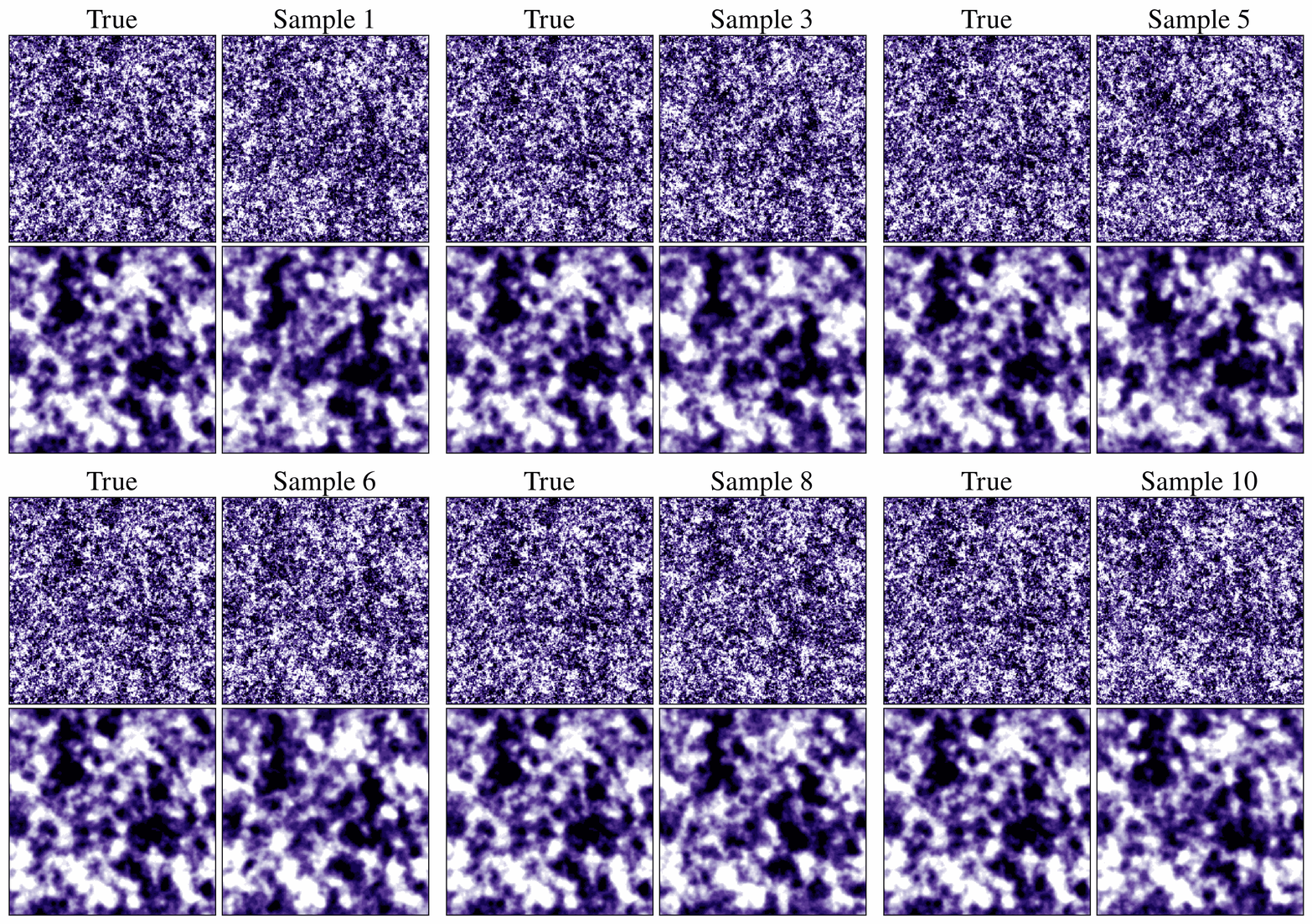
For this fiducial case we show the recovery visually in Fig. 6. The two rows correspond to two different realizations from the test set. In the first column, we show the mock galaxy + 21cm observations. In the second column we show the corresponding true ICs that were used to generate the mock observations. In the final two columns, we show the IC recovery from two calls to TILING, conditioned on the mocks shown in the first column. All fields are 2D slices of width through the corresponding 3D fields that are used in TILING.
From the first column we see again how the bright, observable galaxies preferentially trace the ionized regions where the brightness temperature is negative after mean subtraction. These are hosted by large-scale matter overdensities seen in the second column. Comparing the last two columns to the ground truth shown in the second column, we see that the recovery works very well on large scales though the zoom-in shows small-scale discrepancies (as could be inferred from the CCC shown in the bottom-right panel of Fig. 4).
To highlight the quality of the recovery on large scales, in Fig. 6 we show the same IC fields as in Fig. 6, but smoothed on scales using a second-order Butterworth filter (Butterworth et al. 1930):
| (29) |
The samples from TILING are nearly identical to the ground truth on these scales.
The reader is referred to Appendix C.1 for additional tests of recovery in the fiducial case, where we show the samples’ consistency with the assumed Gaussianity. Furthermore, in Appendix C.3 we perform pixel-based coverage tests for 100 test-set realizations, showing a well-calibrated posterior.
Finally, in Fig. 7 we quantify how our multi-tracer recovery depends on observational effects. In the left column, we show results with and without 21cm foreground wedge removal (i.e., ignoring foreground contamination). We see that the recovery is largely unaffected by wedge excision, due to the fact that in our fiducial set-up, the galaxy maps dominate the constraining power.
In the middle column of Fig. 7 we vary the integration time with SKA-low, showing results for 100h, 1000h, and 10000h. The CCCs are largely unaffected, though the power spectrum recovery does degrade by up to 10% for 100h. This points to the conclusion that although the galaxy maps determine the phases of the recovered ICs in our fiducial multi-tracer set-up, the 21cm maps help to constrain the Fourier amplitudes (i.e., the power spectrum).
This is further evidenced in the right column, where we vary the galaxy UV magnitude threshold. Comparing these curves with the analogous ones in the left column of Fig. 4, we see that the CCC and in particular the values are unchanged. However, the inclusion of 21cm improves the power spectrum recovery, especially for the shallowest survey with . The galaxy-only recovery resulted in mean PSR errors of up to 20%, even at moderate scales of cMpc-1. Adding 21cm maps to the recovery pipeline decreases this error to a few percent.
5 Evolved fields and wedge reconstruction
One powerful application of TILING is to use the inferred posterior samples as initial conditions for cosmological simulations. By ‘‘re-simulating’’ the observed volume, one is able to study its full history, uncorrupted by observational effects. In this section we briefly show one such application: recovering the 21cm foreground wedge.1616 16 In a companion paper, Triantafyllou et al. in prep we go into detail about using TILING to recover galaxy and ionization field evolution of observed volumes.
We use the IC samples produced by TILING, as described in the previous section, as input to 21cmFAST in order to re-simulate the corresponding late-time constrained realizations of the density and 21cm fields. We use slightly different parameter choices for this re-simulation. Specifically, these include: (i) a sharp- filter instead of the default exponential spherical tophat filter from Davies & Furlanetto (2022) for ionizing emissivity fields; (ii) ignoring sub-grid recombinations; (iii) ignoring the contribution of molecularly-cooled galaxies; (iv) assuming a saturated spin temperature (); (v) fixing M⊙; (vi) using a grid resolution of ; and (vii) computing radiation fields using the mean conditional halo abundances rather than the stochastic, discrete source model introduced in v4.
These different modeling choices further test the robustness of , as the output simulator is effectively different than what was used in training. Accurate IC recovery therefore would require TILING to be able to generalize to a different simulation (albeit one done using the same code). Fully quantifying the impact of model misspecification would require testing results against multiple different simulation codes during inference (e.g., Jo et al. 2025; Meriot et al. 2026), and is beyond the scope of this work.
The first row of Fig. 8 shows one example true late-time density field (left panel), alongside a re-simulated posterior sample (middle panel) and the mean across 10 samples (right panel). The mean appears smooth because small scales are weakly constrained, which effectively translates to noise in each realization that averages out in the mean. The random sample and the mean both recover medium to large scales in both fields very well. We provide the corresponding halo mass function in Appendix C as a non-linear quality metric of the recovered density fields.
The second row of Fig. 8 shows similar behavior for the constrained realization of the 21cm signal. We caution again that here we fix the astrophysical parameters, assuming those to be recovered from observations with a comparably smaller uncertainty than the ICs. We will explore co-varying astrophysical parameters in future work.
We quantify the 21cm wedge reconstruction quality in Fig. 9, where we show the 21cm cylindrical power spectra (; in space) from one random test-set realization. In the top row we show the PS of the true intrinsic signal (also without RSDs; left panel) and the mock observation (right panel). The bottom left panel shows the reconstructed as the mean of 10 samples from TILING. Comparing the top and bottom left panels, we see excellent agreement between the true and reconstructed PS, both inside and outside the foreground-dominated wedge.
We further quantify the quality of PS recovery by plotting the cylindrically-averaged CCCs in the bottom right panel. We see that the wedge (purple shaded region) is recovered with accuracy across most of its domain. These results are roughly comparable to Chen et al. (2025a), where they used both approximate models based on EFT as well as a diffusion approach to recover the wedge from foreground-contaminated 21cm mock observations. Our results indicate improved CCCs especially in the direction, demonstrating the strength of using galaxies as an additional tracer. Nevertheless, the inherent differences between approaches (discussed previously) do not allow for a clean, apples-to-apples comparison.
6 Conclusions
The ICs constitute a clean probe for cosmology. Reconstructing them recovers the full temporal evolution of an observed volume. While such reconstruction pipelines are fairly mature at low redshifts, application to the EoR has remained relatively unexplored due to the challenges associated with modeling cosmic radiation fields and a historic dearth of observations.
In order to prepare for ongoing and future large EoR surveys, here we develop TILING, a hybrid pipeline for field-level, multi-tracer reconstruction of IC fields. TILING pairs a point-estimate NN, inspired by Savchenko et al. (2025), with a conditional score-based diffusion model that refines this estimate and provides posterior samples of 3D ICs.We train TILING on combinations of mock galaxy and 21cm maps at , with varying observational effects, quantifying the accuracy of recovery.
Our main results are the following:
- •
High-Fidelity Joint Reconstruction: TILING can reliably constrain ICs down to small scales () by performing joint inference from upcoming galaxy and 21cm observations.
- •
Synergy of galaxy and 21cm maps: We find that most of the constraining power from TILING comes from the galaxy maps, further highlighting the importance for multi-tracer analysis and observations with shared footprints. This is due to the baseline distribution of the SKA, which is not sensitive to the small scales accessible with galaxy maps. The 21cm signal as observed with SKA does aid in recovering the IC power spectra.
- •
Foreground Wedge Recovery: TILING successfully recovers modes of the 21cm power spectrum that were excised due to foreground contamination. The foreground modes can be reconstructed with across most of their domain, under fiducial observational assumptions.
Additionally, our IC reconstruction framework can be used to (i) guide follow-up observations of sub-volumes of interest, (ii) reconstruct the galaxy evolution and corresponding reionization morphology of specific volumes, and (iii) isolate the contribution to reionization by the vast majority of galaxies that will remain unobserved by optical/IR telescopes such as JWST. We address (ii) and (iii) in TILING II (Triantafyllou et al. in prep), where we demonstrate how an IC reconstruction can reduce cosmic variance and predict the joint evolution of reionization and galaxies in specific sub-volumes.
7 Data availability
The data underlying this article will be shared on reasonable request to the corresponding author. Any future publishing of the data will be made available on the corresponding Github page.
Acknowledgements.
We gratefully acknowledge computational resources of the Center for High Performance Computing (CHPC) at SNS. We acknowledge CINECA awards under the ISCRA initiative for providing us access to the LEONARDO supercomputer (IsB30_IC-diff, project no. HP10B1D1F2, PI: Triantafyllou; CNHPC_1497299, project no. 1497299, PI: Mesinger). This project is supported by Italian Ministerial grant PNRR from National Centre for HPC, Big Data and Quantum Computing CUP E53C22000790001, Spoke 3. This work was recognized as the winning poster at E4 Computer Engineering’s "AI, HPC, QUANTUM" event (Milan, September 2025). The authors thank Daniela Breitman for her original contributions to tuesday and her valuable support. We also thank Adrian Liu, Yi Mao and Daniela Breitman for their valuable suggestions that helped improve this work. N.T. expresses his gratitude to David Prelogović for his insights and guidance during the initial phases of this project.References
- Abazajian et al. (2009) Abazajian, K. N., Adelman-McCarthy, J. K., Agüeros, M. A., et al. 2009, ApJS, 182, 543
- Abdalla et al. (2022) Abdalla, E., Abellán, G. F., Aboubrahim, A., et al. 2022, Journal of High Energy Astrophysics, 34, 49
- Aihara et al. (2022) Aihara, H., AlSayyad, Y., Ando, M., et al. 2022, PASJ, 74, 247
- Anderson (1982) Anderson, B. D. O. 1982, Stochastic Process. Appl., 12, 313
- Andrews et al. (2026a) Andrews, A., Jasche, J., Lavaux, G., et al. 2026a, arXiv e-prints, arXiv:2603.20855
- Andrews et al. (2024) Andrews, A., Jasche, J., Lavaux, G., et al. 2024, arXiv e-prints, arXiv:2412.11945
- Andrews et al. (2026b) Andrews, A., Loureiro, A., Jasche, J., et al. 2026b, arXiv e-prints, arXiv:2602.02363
- Ata et al. (2015) Ata, M., Kitaura, F.-S., & Müller, V. 2015, MNRAS, 446, 4250
- Bagla & Padmanabhan (1997) Bagla, J. S. & Padmanabhan, T. 1997, Pramana, 49, 161
- Bagley et al. (2026) Bagley, M. B., Finkelstein, S. L., Rhoads, J., et al. 2026, arXiv e-prints, arXiv:2603.09828
- Bagley et al. (2024) Bagley, M. B., Pirzkal, N., Finkelstein, S. L., et al. 2024, ApJ, 965, L6
- Bartolo et al. (2004) Bartolo, N., Komatsu, E., Matarrese, S., & Riotto, A. 2004, Phys. Rep, 402, 103
- Bayer et al. (2026) Bayer, A. E., Parker, L., Valcin, D., et al. 2026, arXiv e-prints, arXiv:2603.15732
- Behroozi et al. (2019) Behroozi, P., Wechsler, R. H., Hearin, A. P., & Conroy, C. 2019, MNRAS, 488, 3143
- Bennett et al. (2013) Bennett, C. L., Larson, D., Weiland, J. L., et al. 2013, ApJS, 208, 20
- Bernal & Kovetz (2022) Bernal, J. L. & Kovetz, E. D. 2022, A&A Rev., 30, 5
- Bianchini & Maniyar (2025) Bianchini, F. & Maniyar, A. S. 2025, arXiv e-prints, arXiv:2501.13913
- Bianco et al. (2024) Bianco, M., Giri, S. K., Prelogović, D., et al. 2024, MNRAS, 528, 5212
- Blas et al. (2011) Blas, D., Lesgourgues, J., & Tram, T. 2011, J. Cosmology Astropart. Phys., 2011, 034
- Bottema et al. (2025) Bottema, J., Flöss, T., & Daniel Meerburg, P. 2025, J. Cosmology Astropart. Phys., 2025, 030
- Breitman et al. (2025) Breitman, D., Mesinger, A., Murray, S. G., & Acharya, A. 2025, A&A, 703, A130
- Breitman et al. (2026) Breitman, D., Mesinger, A., Murray, S. G., Nikolic, I., & Trotta, R. 2026, arXiv e-prints, arXiv:2606.00219
- Bucher (2015) Bucher, M. 2015, International Journal of Modern Physics D, 24, 1530004
- Butterworth et al. (1930) Butterworth, S. et al. 1930, Wireless Engineer, 7, 536
- Byrohl et al. (2025) Byrohl, C., Nelson, D., Horowitz, B., Lee, K.-G., & Pillepich, A. 2025, A&A, 698, A103
- CD Science Working Group et al. (2026) CD Science Working Group, Bernardi, G., Breitman, D., et al. 2026, arXiv e-prints, arXiv:2606.26435
- Chen et al. (2025a) Chen, S.-F., Chen, K.-F., & Dvorkin, C. 2025a, J. Cosmology Astropart. Phys., 2025, 082
- Chen et al. (2025b) Chen, X., Padmanabhan, N., & Eisenstein, D. J. 2025b, J. Cosmology Astropart. Phys., 2025, 055
- Cortês et al. (2026) Cortês, M., Lahav, O., & Liddle, A. R. 2026, arXiv e-prints, arXiv:2602.13523
- Cranmer et al. (2020) Cranmer, K., Brehmer, J., & Louppe, G. 2020, Proceedings of the National Academy of Science, 117, 30055
- Creminelli et al. (2006) Creminelli, P., Nicolis, A., Senatore, L., Tegmark, M., & Zaldarriaga, M. 2006, J. Cosmology Astropart. Phys., 2006, 004
- Darwish et al. (2021) Darwish, O., Foreman, S., Abidi, M. M., et al. 2021, Phys. Rev. D, 104, 123520
- Davies & Furlanetto (2022) Davies, F. B. & Furlanetto, S. R. 2022, MNRAS, 514, 1302
- Davies et al. (2025) Davies, J. E., Mesinger, A., & Murray, S. 2025, arXiv e-prints, arXiv:2504.17254
- Dawson et al. (2013) Dawson, K. S., Schlegel, D. J., Ahn, C. P., et al. 2013, AJ, 145, 10
- Delchambre et al. (2023) Delchambre, L., Bailer-Jones, C. A. L., Bellas-Velidis, I., et al. 2023, A&A, 674, A31
- Di Cesare et al. (2023) Di Cesare, C., Graziani, L., Schneider, R., et al. 2023, MNRAS, 519, 4632
- Dodelson & Schmidt (2020) Dodelson, S. & Schmidt, F. 2020, Modern Cosmology
- Doeser et al. (2025) Doeser, L., Ata, M., & Jasche, J. 2025, arXiv e-prints, arXiv:2502.13243
- Doeser et al. (2024) Doeser, L., Jamieson, D., Stopyra, S., et al. 2024, MNRAS, 535, 1258
- Dolag et al. (2023) Dolag, K., Sorce, J. G., Pilipenko, S., et al. 2023, A&A, 677, A169
- Dong et al. (2026) Dong, C., Horowitz, B., Bayer, A. E., & Lee, K.-G. 2026, arXiv e-prints, arXiv:2604.26823
- Donnan et al. (2024) Donnan, C. T., McLure, R. J., Dunlop, J. S., et al. 2024, MNRAS, 533, 3222
- Dorent et al. (2025) Dorent, R., Golland, P., & Wells, III, W. 2025, arXiv e-prints, arXiv:2510.20644
- Eisenstein et al. (2011) Eisenstein, D. J., Weinberg, D. H., Agol, E., et al. 2011, AJ, 142, 72
- Eisenstein et al. (2026) Eisenstein, D. J., Willott, C., Alberts, S., et al. 2026, ApJS, 283, 6
- Feng et al. (2018) Feng, Y., Seljak, U., & Zaldarriaga, M. 2018, J. Cosmology Astropart. Phys., 2018, 043
- Ferreira et al. (1998) Ferreira, P. G., Magueijo, J., & Górski, K. M. 1998, ApJ, 503, L1
- Finkelstein et al. (2025) Finkelstein, S. L., Bagley, M. B., Arrabal Haro, P., et al. 2025, ApJ, 983, L4
- Flöss & Meerburg (2024) Flöss, T. & Meerburg, P. D. 2024, JCAP, 2024, 031
- Furlanetto et al. (2006) Furlanetto, S. R., Oh, S. P., & Briggs, F. H. 2006, Phys. Rep, 433, 181
- Gagnon-Hartman et al. (2021) Gagnon-Hartman, S., Cui, Y., Liu, A., & Ravanbakhsh, S. 2021, MNRAS, 504, 4716
- Gagnon-Hartman et al. (2025) Gagnon-Hartman, S., Davies, J. E., & Mesinger, A. 2025, A&A, 699, A131
- Gagnon-Hartman et al. (2026) Gagnon-Hartman, S., Mesinger, A., Nikolić, I., Parlanti, E., & Venturi, G. 2026, arXiv e-prints, arXiv:2602.13389
- Giri et al. (2018) Giri, S. K., Mellema, G., & Ghara, R. 2018, MNRAS, 479, 5596
- Gottloeber et al. (2010) Gottloeber, S., Hoffman, Y., & Yepes, G. 2010, arXiv e-prints, arXiv:1005.2687
- Greig & Mesinger (2018) Greig, B. & Mesinger, A. 2018, MNRAS, 477, 3217
- Harikane et al. (2016) Harikane, Y., Ouchi, M., Ono, Y., et al. 2016, ApJ, 821, 123
- Ho et al. (2020) Ho, J., Jain, A., & Abbeel, P. 2020, Advances in neural information processing systems, 33, 6840
- Hopkins et al. (2012) Hopkins, P. F., Quataert, E., & Murray, N. 2012, MNRAS, 421, 3522
- Horowitz et al. (2019) Horowitz, B., Lee, K.-G., White, M., Krolewski, A., & Ata, M. 2019, ApJ, 887, 61
- Horowitz et al. (2021) Horowitz, B., Zhang, B., Lee, K.-G., & Kooistra, R. 2021, ApJ, 906, 110
- Hutter & Heneka (2026) Hutter, A. & Heneka, C. 2026, A&A, 707, A286
- Inoue et al. (2020) Inoue, A. K., Yamanaka, S., Ouchi, M., et al. 2020, PASJ, 72, 101
- Jamieson et al. (2023) Jamieson, D., Li, Y., de Oliveira, R. A., et al. 2023, ApJ, 952, 145
- Jasche & Kitaura (2010) Jasche, J. & Kitaura, F. S. 2010, MNRAS, 407, 29
- Jasche & Lavaux (2019) Jasche, J. & Lavaux, G. 2019, A&A, 625, A64
- Jasche et al. (2015) Jasche, J., Leclercq, F., & Wandelt, B. D. 2015, J. Cosmology Astropart. Phys., 2015, 036
- Jasche & Wandelt (2013) Jasche, J. & Wandelt, B. D. 2013, MNRAS, 432, 894
- Jensen et al. (2013) Jensen, H., Datta, K. K., Mellema, G., et al. 2013, MNRAS, 435, 460
- Jindal et al. (2023) Jindal, V., Liang, A., Singh, A., Ho, S., & Jamieson, D. 2023, arXiv e-prints, arXiv:2303.13056
- Jo et al. (2025) Jo, Y., Genel, S., Sengupta, A., et al. 2025, ApJ, 991, 120
- Kaiser (1987) Kaiser, N. 1987, MNRAS, 227, 1
- Kakiichi et al. (2024) Kakiichi, K., Egami, E., Fan, X., et al. 2024, COSMOS-3D: A Legacy Spectroscopic/Imaging Survey of the Early Universe, JWST Proposal. Cycle 3, ID. #5893
- Kannan et al. (2022) Kannan, R., Garaldi, E., Smith, A., et al. 2022, MNRAS, 511, 4005
- Kar et al. (2026) Kar, A., Alam, S., & Silk, J. 2026, ApJ, 996, 103
- Kendall & Gal (2017) Kendall, A. & Gal, Y. 2017, arXiv e-prints, arXiv:1703.04977
- Kendall et al. (2017) Kendall, A., Gal, Y., & Cipolla, R. 2017, arXiv e-prints, arXiv:1705.07115
- Kennedy et al. (2024) Kennedy, J., Carr, J. C., Gagnon-Hartman, S., et al. 2024, MNRAS, 529, 3684
- Klypin et al. (2003) Klypin, A., Hoffman, Y., Kravtsov, A. V., & Gottlöber, S. 2003, ApJ, 596, 19
- Komatsu et al. (2003) Komatsu, E., Kogut, A., Nolta, M. R., et al. 2003, ApJS, 148, 119
- Komatsu et al. (2002) Komatsu, E., Wandelt, B. D., Spergel, D. N., Banday, A. J., & Górski, K. M. 2002, ApJ, 566, 19
- Konno et al. (2014) Konno, A., Ouchi, M., Ono, Y., et al. 2014, ApJ, 797, 16
- Lang (2014) Lang, D. 2014, AJ, 147, 108
- Lavaux & Hudson (2011) Lavaux, G. & Hudson, M. J. 2011, MNRAS, 416, 2840
- Lavaux et al. (2019) Lavaux, G., Jasche, J., & Leclercq, F. 2019, arXiv e-prints, arXiv:1909.06396
- Leclercq (2025) Leclercq, F. 2025, arXiv e-prints, arXiv:2509.13435
- Legin et al. (2024) Legin, R., Ho, M., Lemos, P., et al. 2024, MNRAS, 527, L173
- Lemos et al. (2023) Lemos, P., Coogan, A., Hezaveh, Y., & Perreault-Levasseur, L. 2023, 40th International Conference on Machine Learning, 202, 19256
- Lesgourgues (2011) Lesgourgues, J. 2011, arXiv e-prints, arXiv:1104.2932
- Libeskind et al. (2020) Libeskind, N. I., Carlesi, E., Grand, R. J. J., et al. 2020, MNRAS, 498, 2968
- Lin (1991) Lin, J. 1991, IEEE Transactions on Information Theory, 37, 145
- Liu et al. (2014) Liu, A., Parsons, A. R., & Trott, C. M. 2014, Phys. Rev. D, 90, 023018
- Liu & Shaw (2020) Liu, A. & Shaw, J. R. 2020, PASP, 132, 062001
- Maiolino et al. (2020) Maiolino, R., Cirasuolo, M., Afonso, J., et al. 2020, The Messenger, 180, 24
- Maitra et al. (2026) Maitra, S., Kulkarni, G., Arora, V., et al. 2026, arXiv e-prints, arXiv:2601.16263
- Mao et al. (2012) Mao, Y., Shapiro, P. R., Mellema, G., et al. 2012, MNRAS, 422, 926
- Mason et al. (2026) Mason, C. A., Chen, Z., Stark, D. P., et al. 2026, A&A, 705, A114
- Mather et al. (1990) Mather, J. C., Cheng, E. S., Eplee, Jr., R. E., et al. 1990, ApJ, 354, L37
- McAlpine et al. (2022) McAlpine, S., Helly, J. C., Schaller, M., et al. 2022, MNRAS, 512, 5823
- Meisner et al. (2019) Meisner, A. M., Lang, D., Schlafly, E. F., & Schlegel, D. J. 2019, PASP, 131, 124504
- Meriot et al. (2026) Meriot, R., Pritchard, J. R., & Schaeffer, T. 2026, arXiv e-prints, arXiv:2608.14423
- Mertens et al. (2025) Mertens, F. G., Mevius, M., Koopmans, L. V. E., et al. 2025, A&A, 698, A186
- Mesinger (2016) Mesinger, A., ed. 2016, Astrophysics and Space Science Library, Vol. 423, Understanding the Epoch of Cosmic Reionization
- Mesinger & Furlanetto (2007) Mesinger, A. & Furlanetto, S. 2007, ApJ, 669, 663
- Mesinger et al. (2011) Mesinger, A., Furlanetto, S., & Cen, R. 2011, MNRAS, 411, 955
- Meyer et al. (2025) Meyer, R. A., Wang, F., Kakiichi, K., et al. 2025, arXiv e-prints, arXiv:2510.11373
- Mirocha et al. (2017) Mirocha, J., Furlanetto, S. R., & Sun, G. 2017, MNRAS, 464, 1365
- Modi et al. (2018) Modi, C., Feng, Y., & Seljak, U. 2018, J. Cosmology Astropart. Phys., 2018, 028
- Modi et al. (2021) Modi, C., Lanusse, F., Seljak, U., Spergel, D. N., & Perreault-Levasseur, L. 2021, arXiv e-prints, arXiv:2104.12864
- Monaco & Efstathiou (1999) Monaco, P. & Efstathiou, G. 1999, MNRAS, 308, 763
- Morales et al. (2012) Morales, M. F., Hazelton, B., Sullivan, I., & Beardsley, A. 2012, ApJ, 752, 137
- Moriwaki et al. (2024) Moriwaki, K., Beane, A., & Lidz, A. 2024, MNRAS, 530, 3183
- Muñoz et al. (2022) Muñoz, J. B., Qin, Y., Mesinger, A., et al. 2022, MNRAS, 511, 3657
- Munshi et al. (2021) Munshi, F., Brooks, A. M., Applebaum, E., et al. 2021, ApJ, 923, 35
- Munshi et al. (2025) Munshi, S., Koopmans, L. V. E., Mertens, F. G., et al. 2025, A&A, 704, A205
- Murray et al. (2020) Murray, S., Greig, B., Mesinger, A., et al. 2020, The Journal of Open Source Software, 5, 2582
- Murray & Trott (2018) Murray, S. G. & Trott, C. M. 2018, ApJ, 869, 25
- Nebrin et al. (2023) Nebrin, O., Giri, S. K., & Mellema, G. 2023, MNRAS, 524, 2290
- Nguyen et al. (2024) Nguyen, N.-M., Schmidt, F., Tucci, B., Reinecke, M., & Kostić, A. 2024, Phys. Rev. Lett., 133, 221006
- Observations Time Allocation Committee & Community Survey Definition Committees (2025) Observations Time Allocation Committee, R. & Community Survey Definition Committees, C. 2025, arXiv e-prints, arXiv:2505.10574
- Oke & Gunn (1983) Oke, J. B. & Gunn, J. E. 1983, ApJ, 266, 713
- Ono et al. (2024) Ono, V., Park, C. F., Mudur, N., et al. 2024, ApJ, 970, 174
- O’Shea et al. (2015) O’Shea, B. W., Wise, J. H., Xu, H., & Norman, M. L. 2015, ApJ, 807, L12
- Ouchi et al. (2018) Ouchi, M., Harikane, Y., Shibuya, T., et al. 2018, PASJ, 70, S13
- Pallottini et al. (2022) Pallottini, A., Ferrara, A., Gallerani, S., et al. 2022, MNRAS, 513, 5621
- Park et al. (2019) Park, J., Mesinger, A., Greig, B., & Gillet, N. 2019, MNRAS, 484, 933
- Parker et al. (2025) Parker, L., Bayer, A. E., & Seljak, U. 2025, J. Cosmology Astropart. Phys., 2025, 039
- Paszke et al. (2019) Paszke, A., Gross, S., Massa, F., et al. 2019, arXiv e-prints, arXiv:1912.01703
- Perez et al. (2023) Perez, L. A., Malhotra, S., Rhoads, J. E., & Wold, I. G. B. 2023, ApJ, 949, 3
- Planck Collaboration et al. (2016) Planck Collaboration, Ade, P. A. R., Aghanim, N., et al. 2016, A&A, 594, A17
- Planck Collaboration et al. (2020a) Planck Collaboration, Aghanim, N., Akrami, Y., et al. 2020a, A&A, 641, A6
- Planck Collaboration et al. (2020b) Planck Collaboration, Aghanim, N., Akrami, Y., et al. 2020b, A&A, 641, A5
- Planck Collaboration et al. (2020c) Planck Collaboration, Akrami, Y., Arroja, F., et al. 2020c, A&A, 641, A9
- Prelogović & Mesinger (2023) Prelogović, D. & Mesinger, A. 2023, MNRAS, 524, 4239
- Prelogović et al. (2022) Prelogović, D., Mesinger, A., Murray, S., Fiameni, G., & Gillet, N. 2022, MNRAS, 509, 3852
- Pritchard & Loeb (2012) Pritchard, J. R. & Loeb, A. 2012, Reports on Progress in Physics, 75, 086901
- Qin et al. (2020) Qin, Y., Mesinger, A., Park, J., Greig, B., & Muñoz, J. B. 2020, MNRAS, 495, 123
- Qin et al. (2024) Qin, Y., Mesinger, A., Prelogović, D., et al. 2024, arXiv e-prints, arXiv:2412.00799
- Savchenko et al. (2025) Savchenko, O., Abellán, G. F., List, F., Anau Montel, N., & Weniger, C. 2025, arXiv e-prints, arXiv:2502.03139
- Savchenko et al. (2024) Savchenko, O., List, F., Abellán, G. F., Montel, N. A., & Weniger, C. 2024, arXiv preprint arXiv:2410.15808
- Sawala et al. (2022) Sawala, T., McAlpine, S., Jasche, J., et al. 2022, MNRAS, 509, 1432
- Schmittfull et al. (2017) Schmittfull, M., Baldauf, T., & Zaldarriaga, M. 2017, Phys. Rev. D, 96, 023505
- Scoccimarro (1998) Scoccimarro, R. 1998, MNRAS, 299, 1097
- Scott & Smoot (2010) Scott, D. & Smoot, G. F. 2010, arXiv e-prints, arXiv:1005.0555
- Seljak et al. (2017) Seljak, U., Aslanyan, G., Feng, Y., & Modi, C. 2017, J. Cosmology Astropart. Phys., 2017, 009
- Shallue & Eisenstein (2023) Shallue, C. J. & Eisenstein, D. J. 2023, MNRAS, 520, 6256
- Sheth & Tormen (1999) Sheth, R. K. & Tormen, G. 1999, MNRAS, 308, 119
- Silk & Rees (1998) Silk, J. & Rees, M. J. 1998, A&A, 331, L1
- Sirko (2005) Sirko, E. 2005, ApJ, 634, 728
- Smoot et al. (1992) Smoot, G. F., Bennett, C. L., Kogut, A., et al. 1992, ApJ, 396, L1
- Sobacchi & Mesinger (2013) Sobacchi, E. & Mesinger, A. 2013, MNRAS, 432, 3340
- Sohl-Dickstein et al. (2015) Sohl-Dickstein, J., Weiss, E., Maheswaranathan, N., & Ganguli, S. 2015, in International conference on machine learning, PMLR, 2256–2265
- Song et al. (2020) Song, Y., Sohl-Dickstein, J., Kingma, D. P., et al. 2020, arXiv e-prints, arXiv:2011.13456
- Sorce et al. (2021) Sorce, J. G., Dubois, Y., Blaizot, J., et al. 2021, MNRAS, 504, 2998
- Sorce et al. (2016) Sorce, J. G., Gottlöber, S., Yepes, G., et al. 2016, MNRAS, 455, 2078
- Sorce et al. (2026) Sorce, J. G., McGee, S. L., Dubois, Y., et al. 2026, arXiv e-prints, arXiv:2603.23606
- Sridhar (2023) Sridhar, S. 2023, SKAO staged delivery, array assemblies and layouts, Technical report SKAO-TEL-0002299, SKAO
- Stefanon et al. (2021) Stefanon, M., Bouwens, R. J., Labbé, I., et al. 2021, ApJ, 922, 29
- Steinwandel et al. (2026) Steinwandel, U. P., McAlpine, S., Stiskalek, R., et al. 2026, arXiv e-prints, arXiv:2606.10028
- Storey-Fisher et al. (2024) Storey-Fisher, K., Hogg, D. W., Rix, H.-W., et al. 2024, ApJ, 964, 69
- Sun & Furlanetto (2016) Sun, G. & Furlanetto, S. R. 2016, MNRAS, 460, 417
- Talts et al. (2018) Talts, S., Betancourt, M., Simpson, D., Vehtari, A., & Gelman, A. 2018, arXiv e-prints, arXiv:1804.06788
- Tweed et al. (2017) Tweed, D., Yang, X., Wang, H., et al. 2017, ApJ, 841, 55
- Umeda et al. (2025) Umeda, H., Ouchi, M., Kikuta, S., et al. 2025, ApJS, 277, 37
- Venditti et al. (2023) Venditti, A., Graziani, L., Schneider, R., et al. 2023, MNRAS, 522, 3809
- Villaescusa-Navarro (2018) Villaescusa-Navarro, F. 2018, Pylians: Python libraries for the analysis of numerical simulations, Astrophysics Source Code Library, record ascl:1811.008
- Vrbanec et al. (2020) Vrbanec, D., Ciardi, B., Jelić, V., et al. 2020, MNRAS, 492, 4952
- Wang et al. (2014) Wang, H., Mo, H. J., Yang, X., Jing, Y. P., & Lin, W. P. 2014, ApJ, 794, 94
- Wang et al. (2016) Wang, H., Mo, H. J., Yang, X., et al. 2016, ApJ, 831, 164
- Wang et al. (2024) Wang, Z., Shi, F., Yang, X., et al. 2024, Sci. China Phys. Mech. Astron., 67, 219513
- Weinberg et al. (2013) Weinberg, D. H., Mortonson, M. J., Eisenstein, D. J., et al. 2013, Phys. Rep, 530, 87
- Wold et al. (2024) Wold, I. G. B., Malhotra, S., Rhoads, J. E., Tilvi, V., & Gabrielpillai, A. 2024, AJ, 167, 157
- Xu et al. (2016a) Xu, H., Norman, M. L., O’Shea, B. W., & Wise, J. H. 2016a, ApJ, 823, 140
- Xu et al. (2016b) Xu, H., Wise, J. H., Norman, M. L., Ahn, K., & O’Shea, B. W. 2016b, ApJ, 833, 84
- Zhou & Mao (2024) Zhou, M. & Mao, Y. 2024, ApJ, 965, 31
- Zier et al. (2025) Zier, O., Kannan, R., Smith, A., et al. 2025, MNRAS, 544, 410
Appendix A SKA observations
Here, we show how different filtering schemes in space visually affect the SKA 21cm observation. The top left panel of Fig. 10 shows an example intrinsic1717 17 Note that in this appendix we refer to “intrinsic” as the RSDs-free signal, where the noise is added for this comparison. signal from our dataset, using only one slice of the simulation at corresponding to depth in the LoS. After adding noise to the signal in space (as described in Sect. 2.3), transforming directly back to real space without any additional processing results in a highly degraded signal, as illustrated in the second panel of Fig. 10. This effect could compromise the performance of the NN as features may become difficult to extract.


For this reason, we attempted to weight the -space modes to reveal structure in the following way for each -space cell at fixed frequency channel :
| (30) |
where is the unfiltered 2D signal in -space, is the filtered one, and are the weights of the specific normalization. We divide by the sum of the weights to prevent artificial explosion or suppression of the signal’s amplitude.
We test two distinct approaches. The first is an inverse-variance transform, where each cell was divided by its variance 1818 18 where we used a factor of 2 to account for the total variance (real and imaginary parts) (see Sect. 2.3), resulting in high signal-to-noise cells contributing more to the Fourier transform. The second is Wiener filtering where the power spectrum of the final field matches the power spectrum of the intrinsic signal, , where . This transformation is prior-dependent, as it requires assuming a power spectrum for the intrinsic signal , that is not observationally known. For this reason, we calculated the median amplitude of the intrinsic 21cm signal in each cell, over the prior range of astrophysical parameters in Triantafyllou et al. in prep, which can be seen in Fig. 11. The resulting signal in real space can be seen in the lower-right panel of Fig. 10, showing more details than the inverse-variance transform but less prominent structure compared to the intrinsic one. TILING was indifferent to the choice of these weightings. We chose the inverse variance as a physically motivated, prior-independent choice.
We also present how different choices of thermal noise affect the mock observed SKA signal. In the main text, we established a fiducial value of , as illustrated in the bottom-left panel of Fig. 12. Figure 12 visually demonstrates the differences in the signal in the plane of the sky for averaged over in the LoS direction. The top panel displays two perturbations around the fiducial value (100 and 10000h). The 100h observation shows a significant reduction in visible structure, while the 1000 and 10000 cases are visibly similar. Furthermore, adopting the SKA AA4 configuration does not lead to a visible improvement in morphological clarity, as seen in the bottom right panel.
Appendix B Network architecture
| Layer | Input | I/O dim | Param # |
| Input data | - | - | |
| C1 | Input data | ||
| A1 | previous | " | - |
| C2 | " | " | 27,680 |
| B1 | " | " | 64 |
| A2 | " | " | - |
| Downsample | |||
| D1 | " | 8,224 | |
| B2 | " | " | 64 |
| A3 | " | " | " |
| C3 | " | " | 27,680 |
| B3 | " | " | 64 |
| A4 | " | " | " |
| C4 | " | " | 27,680 |
| B4 | " | " | 64 |
| A5 | " | " | " |
| Downsample | |||
| D2 | " | 8,224 | |
| B5 | " | " | 64 |
| A6 | " | " | " |
| C5 | " | " | 27,680 |
| B6 | " | " | 64 |
| A7 | " | " | " |
| C6 | " | " | 27,680 |
| B7 | " | " | 64 |
| A8 | " | " | " |
| Upsample | |||
| U1 | " | 8,224 | |
| B8 | " | " | 64 |
| A9 | " | " | " |
| C7 | concat A2 | 55,328 | |
| B9 | " | " | 64 |
| A10 | " | " | " |
| C8 | " | " | 27,680 |
| B10 | " | " | 64 |
| A11 | " | " | " |
| Upsample | |||
| U2 | " | 8,224 | |
| B11 | " | " | 64 |
| A12 | " | " | " |
| C9 | concat A5 | 110,656 | |
| A13 | " | " | " |
| C10 | " | " | 1,729 |
| Layer | Meaning |
|---|---|
| C | Convolution with kernel size 3, stride 1 |
| A | LeakyReLU activation function |
| B | Batch normalization (Group for diffusion) |
| D | Convolution with kernel size 2, stride 2 |
| U | Transpose with kernel size 2, stride 2 |
B.1 U-net
As explained in the main text, we employ a two-step hybrid model designed to accurately model both the likelihood and the mapping of the high-dimensional space. Both steps utilize the same underlying three-level U-net architecture with two skip connections, the details of which are summarized in Table 2. From left to right, the table columns show the layer type and the input to each layer. The input is always the output of the preceding layer, except at the skip connections where previous intermediate outputs are concatenated (abbreviated as "concat. A2" and "concat. A5").
For the second step of the hybrid model, this U-net is augmented with a Fourier time embedding added before every activation function. We experimented with various placements of this embedding, finding that this configuration yielded the best performance. We also explored several architecture modifications: replacing the standard convolutional blocks with residual blocks (following Song et al. 2020) or increasing the number of baseline feature maps from 32 to 64 did not produce noticeable improvements. Consequently, we selected 32 feature maps as the most computationally efficient choice. The model was trained using a batch size of 8, distributed across the available GPUs.
B.2 Hybrid versus single architecture and additional observational scenarios
Here we show the resulting ICs inference using each part of our two-step hybrid and demonstrate its increased performance. In Fig. 13 the resulting is shown from eight observational scenarios labeled across the x axis. From left to right the observational scenarios are: (i) a single tracer inference only considering galaxy observations considering all galaxies residing in halos of ; (ii) a single-tracer scenario considering only the intrinsic 21cm signal; (iii) a multi-tracer scenario considering both of the previously mentioned tracers; (iv) the same as the previous scenario adding the effect of RSDs; (v) the same as before but with an ; (vi) same as before with the 21cm signal being degraded due to noise addition corresponding to 64000h SKA AA* observation; (vii) same as before after removing a foreground wedge from the 21cm signal and (viii) same as before but with a worse of -19 and a 6400h observation. By looking at the first four columns it is evident that there is significant complementary information in the galaxy and 21cm fields, which is inaccessible under the realistic observational scenarios detailed in the main text under current observational limitations.
Three different inference schemes are shown with different colors, with TILING shown in black. In all cases TILING outperforms simple diffusion (orange) or is equivalent. The teal-colored markers correspond to a model trained only with the first part of the model showing a better . However, this performance does not capture the full picture as other statistics such as the power spectra, the PDF (with skewness and kurtosis of -0.15 -0.13) and bispectra were deviating significantly from the target ICs. Furthermore, TILING outperforms the NGPE in the CCC when its MAP is considered (see also Savchenko et al. 2025 for the MAP behavior compared to the samples on the CCCs).
Appendix C Statistical tests of recovery
In Sect. 5 we performed recovery tests in the evolved space at . Here, we expand upon those results by conducting rigorous statistical diagnostics. These include field-level Gaussianity checks and coverage tests applied directly to the reconstructed ICs, alongside validation of the HMFs derived from re-simulating the posterior samples of the fiducial model.
C.1 Gaussianity and PNGs
Throughout this work, we assume purely Gaussian ICs. Hence, our reconstruction should be able to preserve this Gaussianity, even though nowhere in the loss function or validation it was explicitly stated.
We evaluate the Gaussianity requirement in Fig. 14 by plotting the voxel PDF sampled from a test-set sample. Apart from the distributions being visually closely aligned, we use the three metrics on the panel to quantify their similarity. First, the skewness and kurtosis (the third and fourth standardized moments) are negligible ( for both), confirming the samples are Gaussian for all practical purposes. Second, we further quantify this minimal deviation using the base-two Jensen-Shannon divergence (JS; e.g., Lin 1991; Dorent et al. 2025), which offers a robust framework to quantify this minimal deviation. For two probability distributions, and , the JS is defined as:
| (31) |
where represents the average distribution, and the (base-two) Kullback-Leibler divergence is given by:
| (32) |
The metric is bounded within , where a value of 0 indicates identical distributions and 1 signifies completely disjoint profiles. Notably, our reconstructed fields yield a JS of , indicating that the recovered PDF is practically identical to the true distribution.
Beyond validating the pipeline’s fidelity, the precision with which the framework preserves this baseline Gaussianity serves as a critical indicator of its capacity to detect PNGs. As noted in the introduction, field-level IC reconstruction offers a powerful avenue for placing constraints on early-universe non-Gaussian physics. To evaluate the framework’s capability to constrain PNGs, we measure selected three-point statistics of the fields.
The standard bispectrum, , measures the three-point correlation function in Fourier space. For a discrete field, it is estimated by averaging over all valid triangular configurations that satisfy the closed-triangle condition :
| (33) |
where is the number of fundamental triangles falling within the specified -shells. Hereafter, we refer to the bispectrum as the reduced bispectrum, which has a weaker dependence on cosmology and scale, and is defined as:
| (34) |
where represents the matter power spectrum at wavenumber .
Using the Pylians3 package (Villaescusa-Navarro 2018)2020 20 https://github.com/franciscovillaescusa/Pylians3, we compute bispectra for a random test-set realization along with 10 posterior samples displayed in Fig. 15. Specifically, we evaluated two distinct triangular configurations: the equilateral bispectrum () as a function of wavenumber (upper panel), and the angular dependence of the bispectrum for a fixed pair of large- and small-scale modes (lower panel). For the latter, fixing the magnitudes of and along with their angular separation uniquely determines the third vector’s magnitude, , via the closed-triangle condition. Because of the simulation box’s discreteness and cosmic variance, the bispectrum exhibits inherent scatter even for purely Gaussian fields. To establish this baseline, we calculate the empirical mean and variance of the Gaussian bispectra across the entire 2000 realizations of the simulation suite. These are represented by the gray shaded regions in Fig. 15, which define the expected scatter boundaries under Gaussianity.
The true bispectrum realization is shown as the black dashed line while the samples’ mean and 1 is shown with the teal solid line and shaded regions respectively. For both configurations, the posterior samples demonstrate statistical consistency as their empirical mean remains well within the envelope of the expected Gaussian scatter.2121 21 We note that this is a potential indication of PNG recovery but it remains a sanity check in our idealized Gaussian scenario.
C.2 Halo mass function
In Sect. 5 we showed the reconstructed density field and 21cm field at . In Fig. 16, we provide the halo mass function (HMF) as an additional summary of re-simulated quantities. The true HMF of one test-set realization (teal) is displayed along with the mean and of 10 samples (solid lines and shaded regions respectively) and a Sheth-Tormen HMF (Sheth & Tormen 1999) as a reference. The samples closely match the truth and the reference for the small masses, as expected, due to the correct statistics of the ICs explored in the previous paragraphs. At higher masses, the samples showcase more uncertainty, associated with the densest regions and their dynamical histories. Notably, the single peak in the true HMF in the high-mass end corresponds to one halo under the simulation setup. This halo is successfully reconstructed in most of the posterior samples as indicated by the black line.
C.3 Posterior coverage tests
To further verify the validity of our posteriors across different test-set realizations (in addition to the PSRs and CCCs detailed in Sect. 4), we perform coverage tests.
Coverage tests measure how well an approximate posterior (being a product of an implicit likelihood formalism such as in our case) traces the exact under a single idea: how well the posterior traces the prior when data are drawn from the prior predictive distribution. That is, the prior- and data-averaged posterior should equal the prior:
| (35) |
Equation 35 is an identity when the approximate posterior is replaced with the exact posterior . To evaluate self-consistency under this identity, coverage tests check whether the ground-truth parameters fall within a credible region of a given credibility level of the approximate posterior exactly of the time (yielding an empirical cumulative distribution function; ECDF). In other words, they check whether the ground-truth parameters fall at the edge of an credible region with a uniform probability across all credibility levels (hereafter referred to as “coverage per bin” or EPDF, serving as the empirical probability density function counterpart of the ECDF).
The definition of a credible region is non-unique across implementations, as it relies on a credible region generator (where is a subset of the parameter domain) whose sole defining condition is:
| (36) |
Simulation-based calibration (SBC; Talts et al. 2018) is essentially using a “scanning” credible region generator (i.e., the ranks) for marginal distributions (and so limited to 1D posteriors), whereas in tests of accuracy with random points (TARP; Lemos et al. 2023) they prove that a positionable credible region generator (depending on d) provides a necessary and sufficient condition for good coverage in arbitrary dimensions, but under implementation constraints while affected by the curse of dimensionality.
However in our case of parameter reconstruction it is not possible to examine each individual parameter. Furthermore, for a coverage test multiple samples from multiple realizations are required. Because of the dimensionality of the problem and expensive sampling, we make the following approximation: voxels in the realizations are different parameters during inference, but here we assume they can be treated as one single effective parameter due to the ergodic nature of the ICs2222 22 This approximation holds as long as our effective samples are not correlated.. To this end, we sample once for 100 test-set realizations and randomly select voxel locations to act as different effective parameter ground truths (one per test-set realization). In each test-set realization, we find the first 1000 values that are closest to the corresponding . Then, we treat the values of the sample in these voxel positions as the effective samples of . This results in 100 ground truths with 1000 samples in each case, with which we perform coverage tests.
In Fig. 17 both SBC and TARP are shown (red and blue respectively) as the EPDF (upper panel), ECDF (middle panel) and the ECDF difference from the ideal 1:1 line (lower panel). In all cases, the results are distributed into bins. In all panels, the expected errors due to sampling variance are shown as the gray shaded regions (1 and 2), and are calculated based on the uniformity condition of the EPDF. That is, for simulations, for each bin, this is a series of Bernoulli trials, i.e. it follows a binomial distribution, where and where and the number of samples per bin. The same holds for the ECDF, just by changing the probability of success to where is the th bin. For TARP, we also show the estimated 1 and 2 regions from bootstrapping (blue shaded regions), that is, performing the same TARP test 100 times, for 100 selected ground truths with resampling. Both the SBC and TARP fall well within the region, indicating a well calibrated posterior.