跳到论文正文
W Papers独立论文阅读器 arXiv:2609.08877 论文正文 计算阅读时间 · 0%
引用这篇论文根据当前论文元数据生成,正式投稿前建议核对。


License: CC BY 4.0
arXiv:2609.08877v1 [math.OC] 08 Sep 2026

Equilibria for Time-inconsistent Regular-singular Control Problems

Yuting Jia ††thanks: Department of Mathematical Sciences, Tsinghua University, Beijing 100084, China. jyt22@mails.tsinghua.edu.cn, corresponding author    Zongxia Liang ††thanks: Department of Mathematical Sciences, and Center for Insurance and Risk Management, School of Economics and Management, Tsinghua University, Beijing, China. liangzongxia@tsinghua.edu.cn    Xiaodong Luo ††thanks: Department of Mathematical Sciences, Tsinghua University, Beijing 100084, China. luoxd21@mails.tsinghua.edu.cn
Abstract

This paper studies a time-inconsistent mixed regular-singular control problem in continuous time with non-exponential discount. We seek time-consistent equilibria in an intrapersonal game framework and propose a novel definition of regular-singular equilibrium where both regular and singular controls are unified via control laws. We establish a verification theorem to provide a sufficient condition of the equilibrium. Furthermore, we propose a novel concept of mild equilibrium for which perturbations are applied separately to the regular and singular control and give the mild verification theorem. We illustrate the applicability of the theory to the effort and dividend problem and obtain an explicit equilibrium depending on the effort and dividend thresholds under a mixture of exponential discount functions and a pseudo-exponential discount function by solving the extended Hamilton–Jacobi–Bellman (HJB) system. The convexity of the value function is rigorously established, and the equilibrium conditions are verified. In addition, we establish the existence of the effort and dividend thresholds under a mixture of exponential discount functions. Numerical results reveal the impacts of exogenous parameters on the effort and dividend thresholds and the equilibrium value function, along with their economic implications.

Keywords: Time-inconsistency; Regular-singular control law; Non-exponential discount; Equilibrium; Mild equilibrium; Effort and dividend problem.

1 Introduction

Time inconsistency, which was first systematically examined by Samuelson (1937), is a pervasive feature in many financial and economic decision-making problems. It commonly originates from non-exponential discounting, mean-variance objective, and distorted probabilities, etc. In time-inconsistent problems, Bellman’s principle of optimality no longer holds, and consequently, a strategy that is deemed optimal today may no longer appear optimal when reconsidered from a future perspective and conventional dynamic programming techniques are not directly applicable. Strotz (1955) proposed both pre-commitment and equilibrium strategies to address the inconsistency. Under the former, the agent formulates a plan that is optimal from today’s perspective and commits to it, disregarding any future incentives to deviate ( cf.Bajeux-Besnainou and Portait (1998), Li and Ng (2000), Richardson (1989), Zhou and Li (2000)). In the latter approach, the agent’s strategies are characterized as the equilibrium outcome of an intrapersonal game, in which the players are the successive temporal selves of the same individual. However, given that insisting on a pre-committed strategy that a future self would find suboptimal is behaviorally untenable, we pursue time-consistent equilibria in this paper.

The intrapersonal game treatment of time inconsistency dates back to Strotz (1955), who treated the successive incarnations of the same decision maker are treated as noncooperative players within a dynamic game and sought Nash subgame-perfect equilibrium points. Marín-Solano and Navas (2010) derived a modified HJB equation to solve an optimal consumption and investment problem with the non-constant discount rate. The precise definition of the equilibrium concept in continuous time was first provided by Ekeland and Lazrak (2006); Ekeland and Lazrak (2010) and Ekeland and Pirvu (2008). Ekeland et al. (2012) applied the equilibrium framework to the portfolio management problem under hyperbolic discounting. Following their definition, Björk and Murgoci (2010) further advanced the game-theoretic framework by deriving an extended HJB system, along with a corresponding verification theorem, for a broad class of Markovian time-inconsistent stochastic control problems. Björk et al. (2014) extended the equilibrium framework to the mean-variance portfolio optimization problem with state-dependent risk aversion. Around the same time, Hu et al. (2012); Hu et al. (2017) developed a rigorous equilibrium theory for time-inconsistent stochastic linear–quadratic control problems. Christensen and Lindensjö (2018); Christensen and Lindensjö (2020), Ebert et al. (2020) extend the framework from stochastic control to time-inconsistent optimal stopping problems. Beyond that, the equilibrium framework has been widely applied across a broad range of time-inconsistent problems, including portfolio selection (e.g., Kryger and Steffensen (2010), Dong and Sircar (2014)), reinsurance–investment problems (e.g., Li et al. (2015), Liang and Song (2015) Lin and Qian (2016)), regular dividend problems (e.g., Cao et al. (2025), Hu and Zhou (2025), Li et al. (2016), Zhao et al. (2014)).

It should be noted that the aforementioned literature is confined to regular control problems, whereas research on time‑inconsistent singular control has only begun to emerge in recent years. In contrast to regular control, the singular control is characterized as a nondecreasing ca´\acute{a}dla´\acute{a}g process. The theoretical foundation of time‑inconsistent singular control was first laid by Liang et al. (2024), who established an equilibrium framework for singular control with nonexponential discounting, defined the concept of equilibrium singular control law, derived an extended HJB system, and proved the corresponding verification theorem and the existence of classical solutions. This framework was subsequently extended by Bodnariu et al. (2025), who introduced the notion of mild thresholds and generalized the equilibrium to broader classes of singular controls. In a parallel strand, Dai et al. (2024) proposed an alternative equilibrium definition for a time‑inconsistent mean–variance portfolio selection problem with transaction costs and characterized the associated singular trading strategies. Hereafter, the theory of time‑inconsistent singular control has been further developed and brought to bear on various financial problems: Liang and Luo (2025) studied a singular reinsurance Stackelberg game under the mean–variance criterion, while Cao et al. (2026a) examined the singular dividend problems under the mean-variance criterion. In very recent work, Cao et al. (2026b) investigated an equilibrium singular dividend control problem arising from ambiguity aggregation of heterogeneous discount rates, and Dai et al. (2026) studied equilibrium singular control problems with a running minimum process under non-exponential discounting.

Although the equilibrium theory of time‑inconsistent singular control has advanced considerably in recent years, singular interventions alone cannot adequately address many practical decision problems. In fact, in many real-world settings–including finance, insurance, resource management, and inventory control–decision makers routinely employ both continuous adjustments and singular interventions, which naturally gives rise to mixed regular–singular control problems (see, e.g., Chen et al. (2021), Jgaard and Taksar (1999),Guan et al. (2023), Guo et al. (2004), Qiu et al. (2023), Taksar and Zhou (1998)). However, the existing literature remains largely restricted to time‑consistent settings, and a general equilibrium framework for mixed regular–singular control problems under non‑exponential discounting has yet to be established. Most recently, Liang and Young (2026) and Liang et al. (2026) investigate a class of regular–singular control problems under the mean–variance criterion. Non‑exponential discounting, as one of the major causes of time inconsistency in the literature (cf. Ekeland and Pirvu (2008), Harris and Laibson (2001)), is also worthy of investigation. This paper aims to fill this gap.

In this paper, we study a time-inconsistent mixed regular-singular control problem in continuous time with non-exponential discount and seek time-consistent equilibria in an intrapersonal game framework. The main contributions of this paper are summarized as follows.

First, we establish a closed-loop equilibrium framework for the general class of time-inconsistent regular–singular stochastic control problem in continuous time with non-exponential discount, based on a unified control-law formulation. The drift and volatility coefficients of the controlled state process are jointly influenced by both regular and singular controls. Building upon the frameworks of Björk et al. (2017) and Liang et al. (2024), both the regular and singular controls are simultaneously and jointly generated by their corresponding control laws. Within our framework, control laws are equivalently defined as mappings on the augmented state space: the regular control law maps into the regular control space, whereas the singular control law is equivalently a mapping into the binary-valued set of “waiting” and “intervening”. The regular and singular control laws are unified via the Skorohold reflection problems. Since the regular and singular controls jointly affect both the drift and volatility coefficients of the controlled state process, they are intrinsically coupled; our framework therefore perturbs them simultaneously. This approach stands in contrast to Liang and Yuan (2023), in which the regular control and the stopping time are perturbed separately in a mixed control problem of regular control and stopping. Similar to Liang et al. (2024), the perturbation we introduce is of an open-loop form. We seek time-consistent weak equilibria in an intrapersonal game framework and the corresponding equilibrium definition is presented in Definition 2.6.

Second, we establish a verification theorem (3.1) that provides a sufficient condition for an admissible regular-singular control law to constitute an equilibrium. Specifically, under suitable regularity and integrability conditions, any admissible control law derived from a solution to the extended HJB system qualifies as an equilibrium. This theorem thus bridges the gap between the abstract equilibrium definition and its practical implementation.

Furthermore, similar to Liang and Yuan (2023), we propose a novel concept of mild equilibrium (see Definition 4.1), in which perturbations are applied separately to the regular and singular controls. This alternative equilibrium notion accommodates scenarios where the decision maker may deviate in only one type of control at a time, rather than both simultaneously. We also establish the corresponding mild verification theorem (Theorem 4.2), which provides a sufficient condition for an admissible control law to constitute a mild equilibrium. This additional equilibrium concept enriches our theoretical framework and accommodates a broader spectrum of time-inconsistent decision-making scenarios. Together with the standard equilibrium framework, this mild equilibrium concept offers greater flexibility in characterizing time-consistent strategies across different perturbation structures.

Finally, we illustrate the applicability of our theoretical framework through the effort and dividend problem. The firm controls the effort and dividend strategies to minimize the expected total net cost of running the business until failure. By solving the extended HJB system, we obtain explicit equilibrium characterized by the effort and dividend thresholds under two representative discount structures: a mixture of exponential discount functions and a pseudo-exponential discount function. Note that for the time-consistent counterpart, the convexity of the value function follows directly from its optimality; see Jgaard and Taksar (1999, Proposition 1.1). The same conclusion, however, does not apply to the equilibrium value function. For the two discount functions considered in this paper, the convexity of the value function is rigorously established, and the equilibrium conditions are verified. In addition, we establish the existence of the effort and dividend thresholds under the mixture of exponential discount functions. Under mild conditions, the equilibrium policy prescribes exerting the maximal level of effort when the surplus falls below the effort threshold and paying dividends once the surplus exceeds the dividend threshold when the cost for dividend is relatively small; otherwise, when the cost for dividend is relatively large, the equilibrium policy is to pay the dividend once the surplus exceeds the dividend threshold and not to apply effort even if the firm is at the ruin time. The closed-form solutions validate the feasibility of our theoretical framework and provides economically intuitive insights for dynamic corporate finance decisions involving effort allocation and shareholder payouts. Numerical analysis further quantifies the effects of key exogenous parameters on the thresholds and the equilibrium value function under the pseudo-exponential discount function, thereby shedding light on their economic implications.

The remainder of the paper is organized as follows. Section 2 formulates the model of time-inconsistent regular-singular control problems with non-exponential discount and introduce the equilibrium framework. Section 3 establishes a verification theorem. Section 4 provides the concept of mild equilibrium and gives the mild verification theorem. Section 5 applies the theory to the effort and dividend problem. Section 6 presents and discusses some numerical results and sensitivity analysis. The last section concludes this paper.

2 Model formulation

Let (Ω,ℱ,{ℱt}t≥0,ℙ)\left(\Omega,\mathcal{F},\left\{\mathcal{F}_{t}\right\}_{t\geq 0},\mathbb{P}\right) be a filtered complete probability space satisfying the usual conditions and B={Bt}t≥0B=\left\{B_{t}\right\}_{t\geq 0} be a standard one-dimensional Brownian motion on this space.

For any fixed (x,t,y)∈𝒬:=[0,+∞)×[0,+∞)×[0,+∞)(x,t,y)\in\mathcal{Q}:=[0,+\infty)\times[0,+\infty)\times[0,+\infty), the controlled state process Xπ,ξX^{\pi,\xi} under the regular control π\pi and the singular control ξ\xi follows the general stochastic differential equation (abbr. SDE):

(2.1) {dXπ,ξr=μ(Xπ,ξr,r,πr,ξr)dr+σ(Xπ,ξr,r,πr,ξr)dBr−dξr,r∈[t,τx,t,y;π,ξt],Xt−π,ξ=x,\left\{\begin{array}[]{l}\mathrm{d}X^{\pi,\xi}_{r}=\mu\left(X^{\pi,\xi}_{r},r,\pi_{r},\xi_{r}\right)\mathrm{d}r+\sigma\left(X^{\pi,\xi}_{r},r,\pi_{r},\xi_{r}\right)\mathrm{d}B_{r}-\mathrm{d}\xi_{r},\ r\in[t,\tau^{x,t,y;\pi,\xi}_{t}],\\ X^{\pi,\xi}_{t-}=x,\end{array}\right.

where π={πr}r≥t\pi=\left\{\pi_{r}\right\}_{r\geq t} is the regular control, ξ={ξr}r≥t\xi=\left\{\xi_{r}\right\}_{r\geq t} is the singular control which is nondecreasing and ca´\acute{a}dla´\acute{a}g with initial ξt−=y\xi_{t-}=y, and Δ​ξr=ξr−ξr−≤Xr−π,ξ\Delta\xi_{r}=\xi_{r}-\xi_{r-}\leq X_{r-}^{\pi,\xi}. τtx,t,y;π,ξ:=inf{r≥t|Xrπ,ξ=0}\tau^{x,t,y;\pi,\xi}_{t}:=\inf\left\{r\geq t|X^{\pi,\xi}_{r}=0\right\} is the time of bankruptcy, and the drift function μ\mu and the volatility function σ\sigma are exogenously given and deterministic continuous functions on [0,+∞)×[0,+∞)×U×[0,+∞)[0,+\infty)\times[0,+\infty)\times U\times[0,+\infty), where compact set U⊂ℝU\subset\mathbb{R} is the regular control space.

The optimization problem is to find a regular-singular control (π,ξ)(\pi,\xi) that minimizes the objective

J⁡(x,t,y,π,ξ):=\displaystyle J(x,t,y;\pi,\xi):= 𝔼x,t,y​[∫tτtx,t,y;π,ξβ⁡(r−t)​H​(Xrπ,ξ,r,πr,ξr)​dr+∫tτtx,t,y;π,ξβ⁡(r−t)​c​(Xr−π,ξ,r,ξr−)​d​ξr],\displaystyle\mathbb{E}_{x,t,y}\left[\int_{t}^{\tau^{x,t,y;\pi,\xi}_{t}}\beta(r-t)H\left(X_{r}^{\pi,\xi},r,\pi_{r},\xi_{r}\right)\mathrm{d}r+\int_{t}^{\tau^{x,t,y;\pi,\xi}_{t}}\beta(r-t)c\left(X_{r-}^{\pi,\xi},r,\xi_{r-}\right)\mathrm{d}\xi_{r}\right],

where 𝔼x,t,y\mathbb{E}_{x,t,y} denotes the expectation conditioning on Xt−π,ξ=xX^{\pi,\xi}_{t-}=x and ξt−=y\xi_{t-}=y, and ∫tτtx,t,y;π,ξβ⁡(r−t)​c​(Xr−π,ξ,r,ξr−)​d​ξr=∫tτtx,t,y;π,ξβ⁡(r−t)​c​(Xrπ,ξ,r,ξr)​d​ξrc+∑r∈[t,τtx,t,y;π,ξ]β⁡(r−t)​c​(Xr−π,ξ,r,ξr−)​Δ​ξr\int_{t}^{\tau^{x,t,y;\pi,\xi}_{t}}\beta(r-t)c\left(X_{r-}^{\pi,\xi},r,\xi_{r-}\right)\mathrm{d}\xi_{r}=\int_{t}^{\tau^{x,t,y;\pi,\xi}_{t}}\beta(r-t)c\left(X_{r}^{\pi,\xi},r,\xi_{r}\right)\mathrm{d}\xi_{r}^{c}+\sum\limits_{r\in[t,\tau^{x,t,y;\pi,\xi}_{t}]}\beta(r-t)c\left(X_{r-}^{\pi,\xi},r,\xi_{r-}\right)\Delta\xi_{r}, with ξrc\xi_{r}^{c} and Δ​ξr=ξr−ξr−\Delta\xi_{r}=\xi_{r}-\xi_{r-} being the continuous and discrete parts of ξr\xi_{r}. β\beta is a general discount function. Furthermore, we assume the deterministic functions HH, cc and β\beta are exogenously given continuous functions bounded from below. In addition, we assume that c∈C1,0,1​(𝒬)c\in C^{1,0,1}(\mathcal{Q}), and β∈C([0,+∞))\beta\in C([0,+\infty)) is non-negative and nonincreasing with β⁡(0)=1\beta(0)=1. In addition, the cost rate cc should be assumed to stay the same during the jump, i.e.,

(2.2) c⁡(x−a,t,y+a)=c⁡(x,t,y),∀(x,t,y)∈𝒬,a≥0,c(x-a,t,y+a)=c(x,t,y),\ \forall(x,t,y)\in\mathcal{Q},a\geq 0,

or, equivalently, cx​(x,t,y)=cy​(x,t,y),∀(x,t,y)∈𝒬c_{x}(x,t,y)=c_{y}(x,t,y),\forall(x,t,y)\in\mathcal{Q}.

As the discount function might not be exponential, time-inconsistency is involved. In the sense of closed-loop control, we introduce the definition of regular-singular control law. The regular control process π\pi is generated by some regular control law Π=Π⁡(⋅,⋅,⋅)\Pi=\Pi(\cdot,\cdot,\cdot) as a feedback function of the state-time-(singular)control triple as Björk et al. (2017) and Björk et al. (2021), while the singular control process ξ\xi is generated by some singular control law Ξ\Xi as a division of the space 𝒬\mathcal{Q} of state-time-(singular)control triple as Liang and Luo (2025) and Liang et al. (2024). Ξ\Xi is equivalently a mapping from 𝒬\mathcal{Q} into the binary-set of “waiting” and “intervening”. Hence, the admissible regular-singular control law is defined as follows:

Definition 2.1 (Admissible regular-singular control law).

Let Π=Π⁡(⋅,⋅,⋅)\Pi=\Pi(\cdot,\cdot,\cdot) be a UU-valued Borel-measurable function on 𝒬\mathcal{Q}, and Ξ=(WΞ,PΞ)\Xi=\left(W^{\Xi},P^{\Xi}\right) be a Borel-measurable division of 𝒬\mathcal{Q} with WΞW^{\Xi} denoting the waiting region and PΞ=(WΞ)cP^{\Xi}=\left(W^{\Xi}\right)^{c} denoting the action region (the complement of the waiting region). The regular-singular control law (Π,Ξ)\left(\Pi,\Xi\right) is admissible if the following conditions hold:
(a). Given any initial (x,t,y)∈𝒬(x,t,y)\in\mathcal{Q}, the Skorokhod reflection type SDE

{dXΠ,Ξr=μ(XΠ,Ξr,r,Π(XΠ,Ξr,r,ξΠ,Ξr),ξΠ,Ξr)dr+σ(XΠ,Ξr,r,Π(XΠ,Ξr,r,ξΠ,Ξr),ξΠ,Ξr)dBr−dξΠ,Ξr,r∈[t,τx,t,y;Π,Ξt],(XΠ,Ξr,r,ξΠ,Ξr)∈WΞ¯,r∈[t,τx,t,y;Π,Ξt],ξΠ,Ξr=y+∫tr1{(XΠ,Ξl,l,ξΠ,Ξl)∈PΞ}dξΠ,Ξl,r∈[t,τx,t,y;Π,Ξt],Xt−Π,Ξ=x\left\{\begin{array}[]{l}\!\mathrm{d}X^{\Pi,\Xi}_{r}\!\!=\!\mu\!\left(\!X^{\Pi,\Xi}_{r}\!,r,\!\Pi\!\left(\!X^{\Pi,\Xi}_{r}\!,r,\xi^{\Pi,\Xi}_{r}\right)\!,\xi^{\Pi,\Xi}_{r}\right)\!\mathrm{d}r\!+\!\sigma\!\left(\!X^{\Pi,\Xi}_{r}\!,r,\!\Pi\!\left(\!X^{\Pi,\Xi}_{r}\!,r,\xi^{\Pi,\Xi}_{r}\right)\!,\xi^{\Pi,\Xi}_{r}\right)\!\mathrm{d}B_{r}\!\!-\!\mathrm{d}\xi^{\Pi,\Xi}_{r}\!\!,\ r\!\in\![t,\!\tau^{x,t,y;\Pi,\Xi}_{t}],\\ \!\left(\!X^{\Pi,\Xi}_{r}\!,r,\xi^{\Pi,\Xi}_{r}\right)\!\in\!\overline{W^{\Xi}},\ r\!\in\![t,\!\tau^{x,t,y;\Pi,\Xi}_{t}],\\ \!\xi^{\Pi,\Xi}_{r}\!\!=\!y\!+\!\int_{t}^{r}\!1_{\left\{\left(\!X^{\Pi,\Xi}_{l}\!,l,\xi^{\Pi,\Xi}_{l}\right)\in P^{\Xi}\right\}}\!\mathrm{d}\xi^{\Pi,\Xi}_{l}\!\!,\ r\!\in\![t,\!\tau^{x,t,y;\Pi,\Xi}_{t}],\\ \!X^{\Pi,\Xi}_{t-}=x\end{array}\right.

has a unique strong solution (Xx,t,y;Π,Ξ,ξx,t,y;Π,Ξ):=({XrΠ,Ξ}r∈[t,τtx,t,y;Π,Ξ],{ξrΠ,Ξ}r∈[t,τtx,t,y;Π,Ξ])\left(X^{x,t,y;\Pi,\Xi},\xi^{x,t,y;\Pi,\Xi}\right):=\left(\left\{X^{\Pi,\Xi}_{r}\right\}_{r\in[t,\tau^{x,t,y;\Pi,\Xi}_{t}]},\left\{\xi^{\Pi,\Xi}_{r}\right\}_{r\in[t,\tau^{x,t,y;\Pi,\Xi}_{t}]}\right), where τtx,t,y;Π,Ξ:=inf{r≥t|Xrx,t,y;Π,Ξ=0}\tau^{x,t,y;\Pi,\Xi}_{t}:=\inf\left\{r\geq t|X^{x,t,y;\Pi,\Xi}_{r}=0\right\}. The process πx,t,y;Π,Ξ:={Π⁡(XrΠ,Ξ,r,ξΠ,Ξ)}r∈[t,τtx,t,y;Π,Ξ]\pi^{x,t,y;\Pi,\Xi}:=\left\{\Pi\left(X^{\Pi,\Xi}_{r},r,\xi^{\Pi,\Xi}\right)\right\}_{r\in[t,\tau^{x,t,y;\Pi,\Xi}_{t}]} and ξx,t,y;Π,Ξ\xi^{x,t,y;\Pi,\Xi} are respectively the regular control process and singular control process simultaneously generated by the pair of control law (Π,Ξ)(\Pi,\Xi) at initial (x,t,y)∈𝒬(x,t,y)\in\mathcal{Q}.
(b). The strong solution (Xx,t,y;Π,Ξ,ξx,t,y;Π,Ξ)\left(X^{x,t,y;\Pi,\Xi},\xi^{x,t,y;\Pi,\Xi}\right) given in (a) satisfies

𝔼x,t,y​[∫tτtx,t,y;Π,Ξβ⁡(r−t)​|H⁡(Xrx,t,y;Π,Ξ,r,πrx,t,y;Π,Ξ,ξrx,t,y;Π,Ξ)|​dr]<+∞,\displaystyle\mathbb{E}_{x,t,y}\left[\int_{t}^{\tau^{x,t,y;\Pi,\Xi}_{t}}\beta(r-t)\left|H\left(X^{x,t,y;\Pi,\Xi}_{r},r,\pi^{x,t,y;\Pi,\Xi}_{r},\xi^{x,t,y;\Pi,\Xi}_{r}\right)\right|\mathrm{d}r\right]<+\infty,
𝔼x,t,y​[∫tτtx,t,y;Π,Ξβ⁡(r−t)​|c⁡(Xr−x,t,y;Π,Ξ,r,ξr−x,t,y;Π,Ξ)|​d​ξrx,t,y;Π,Ξ]<+∞.\displaystyle\mathbb{E}_{x,t,y}\left[\int_{t}^{\tau^{x,t,y;\Pi,\Xi}_{t}}\beta(r-t)\left|c\left(X^{x,t,y;\Pi,\Xi}_{r-},r,\xi^{x,t,y;\Pi,\Xi}_{r-}\right)\right|\mathrm{d}\xi^{x,t,y;\Pi,\Xi}_{r}\right]<+\infty.

The objective of an admissible regular-singular control law (Π,Ξ)(\Pi,\Xi) is then

(2.3) J⁡(x,t,y,Π,Ξ):=\displaystyle J(x,t,y;\Pi,\Xi):= 𝔼x,t,y[∫tτtx,t,y;Π,Ξβ(r−t)H(Xx,t,y;Π,Ξr,r,πx,t,y;Π,Ξr,ξx,t,y;Π,Ξr)dr\displaystyle\mathbb{E}_{x,t,y}\left[\int_{t}^{\tau^{x,t,y;\Pi,\Xi}_{t}}\beta(r-t)H\left(X^{x,t,y;\Pi,\Xi}_{r},r,\pi^{x,t,y;\Pi,\Xi}_{r},\xi^{x,t,y;\Pi,\Xi}_{r}\right)\mathrm{d}r\right.
+∫tτtx,t,y;Π,Ξβ(r−t)c(Xx,t,y;Π,Ξr−,r,ξx,t,y;Π,Ξr−)dξx,t,y;Π,Ξr],∀(x,t,y)∈𝒬.\displaystyle\left.+\int_{t}^{\tau^{x,t,y;\Pi,\Xi}_{t}}\beta(r-t)c\left(X^{x,t,y;\Pi,\Xi}_{r-},r,\xi^{x,t,y;\Pi,\Xi}_{r-}\right)\mathrm{d}\xi^{x,t,y;\Pi,\Xi}_{r}\right],\ \forall(x,t,y)\in\mathcal{Q}.

Before introducing the equilibrium, we introduce the admissible set of open-loop controls for perturbation:

Definition 2.2 (Admissible regular-singular control pair).

Fix initial (x,t,y)∈𝒬(x,t,y)\in\mathcal{Q}. Let π={πr}r≥t\pi=\{\pi_{r}\}_{r\geq t} be a UU-valued {ℱr}r≥t\{\mathcal{F}_{r}\}_{r\geq t}-progressively measurable process and ξ={ξr}r≥t\xi=\{\xi_{r}\}_{r\geq t} be a nondecreasing ca´\acute{a}dla´\acute{a}g {ℱr}r≥t\{\mathcal{F}_{r}\}_{r\geq t}-adapted process. Then (π,ξ)(\pi,\xi) is called an admissible regular-singular control pair at (x,t,y)(x,t,y) if the following hold:
(a). ξt−=y\xi_{t-}=y, Δ​ξr=ξr−ξr−≤Xr−π,ξ\Delta\xi_{r}=\xi_{r}-\xi_{r-}\leq X_{r-}^{\pi,\xi}, and the SDE (2.1) has a unique strong solution Xπ,ξ={Xrπ,ξ}r∈[t,τtx,t,y;π,ξ]X^{\pi,\xi}=\{X^{\pi,\xi}_{r}\}_{r\in[t,\tau^{x,t,y;\pi,\xi}_{t}]}.
(b). The strong solution Xπ,ξX^{\pi,\xi} in (a) and (π,ξ)(\pi,\xi) satisfies

𝔼x,t,y​[∫tτtx,t,y;π,ξβ⁡(r−t)​|H⁡(Xrπ,ξ,r,πr,ξr)|​dr]<+∞,\displaystyle\mathbb{E}_{x,t,y}\left[\int_{t}^{\tau^{x,t,y;\pi,\xi}_{t}}\beta(r-t)\left|H\left(X_{r}^{\pi,\xi},r,\pi_{r},\xi_{r}\right)\right|\mathrm{d}r\right]<+\infty,
𝔼x,t,y​[∫tτtx,t,y;π,ξβ⁡(r−t)​|c⁡(Xr−π,ξ,r,ξr−)|​d​ξr]<+∞.\displaystyle\mathbb{E}_{x,t,y}\left[\int_{t}^{\tau^{x,t,y;\pi,\xi}_{t}}\beta(r-t)\left|c\left(X_{r-}^{\pi,\xi},r,\xi_{r-}\right)\right|\mathrm{d}\xi_{r}\right]<+\infty.

Denote the set of all admissible regular-singular control pairs at (x,t,y)(x,t,y) by 𝒟x,t,y\mathcal{D}^{x,t,y}.

For any fixed admissible regular-singular control law (Π^,Ξ^)\left(\hat{\Pi},\hat{\Xi}\right), for any (η,u)∈𝒟x,t,y(\eta,u)\in\mathcal{D}^{x,t,y}, if there exist constants h~>0\tilde{h}>0 and M~>0\tilde{M}>0 such that η\eta additionally satisfies

(2.4) η(t+h)−−ηt≤M~​h,a.s.,∀h∈(0,h~),\eta_{(t+h)-}-\eta_{t}\leq\tilde{M}h,\ \text{a.s.},\ \forall h\in(0,\tilde{h}),

and the perturbed regular-singular control pair (πh,ξh)\left(\pi^{h},\xi^{h}\right), ∀h∈(0,h~)\forall h\in(0,\tilde{h}), defined by

(2.5) πrh:={ur,r∈[t,τtx,t,y;u,η∧((t+h)−)],πrXτtx,t,y;u,η∧((t+h)−)u,η,τtx,t,y;u,η∧(t+h),ητtx,t,y;u,η∧((t+h)−);Π^,Ξ^,r∈(τx,t,y;u,ηt∧((t+h)−),τx,t,y;πh,ξht],\displaystyle\pi^{h}_{r}:=\begin{cases}u_{r},&r\in[t,\tau^{x,t,y;u,\eta}_{t}\wedge((t+h)-)],\\ \pi^{X^{u,\eta}_{\tau^{x,t,y;u,\eta}_{t}\wedge((t+h)-)},\tau^{x,t,y;u,\eta}_{t}\wedge(t+h),\eta_{\tau^{x,t,y;u,\eta}_{t}\wedge((t+h)-)};\hat{\Pi},\hat{\Xi}}_{r},&r\in(\tau^{x,t,y;u,\eta}_{t}\wedge((t+h)-),\tau^{x,t,y;\pi^{h},\xi^{h}}_{t}],\end{cases}
ξrh:={ηr,r∈[t,τtx,t,y;u,η∧((t+h)−)],ξrXτtx,t,y;u,η∧((t+h)−)u,η,τtx,t,y;u,η∧(t+h),ητtx,t,y;u,η∧((t+h)−);Π^,Ξ^,r∈(τx,t,y;u,ηt∧((t+h)−),τx,t,y;πh,ξht],\displaystyle\xi^{h}_{r}:=\begin{cases}\eta_{r},&r\in[t,\tau^{x,t,y;u,\eta}_{t}\wedge((t+h)-)],\\ \xi^{X^{u,\eta}_{\tau^{x,t,y;u,\eta}_{t}\wedge((t+h)-)},\tau^{x,t,y;u,\eta}_{t}\wedge(t+h),\eta_{\tau^{x,t,y;u,\eta}_{t}\wedge((t+h)-)};\hat{\Pi},\hat{\Xi}}_{r},&r\in(\tau^{x,t,y;u,\eta}_{t}\wedge((t+h)-),\tau^{x,t,y;\pi^{h},\xi^{h}}_{t}],\end{cases}

and the corresponding state process

(2.6) Xrπh,ξh={Xru,η,r∈[t,τtx,t,y;u,η∧((t+h)−)],XrXτtx,t,y;u,η∧((t+h)−)u,η,τtx,t,y;u,η∧(t+h),ητtx,t,y;u,η∧((t+h)−);Π^,Ξ^,r∈(τx,t,y;u,ηt∧((t+h)−),τx,t,y;πh,ξht],\displaystyle X^{\pi^{h},\xi^{h}}_{r}=\begin{cases}X^{u,\eta}_{r},&r\in[t,\tau^{x,t,y;u,\eta}_{t}\wedge((t+h)-)],\\ X^{X^{u,\eta}_{\tau^{x,t,y;u,\eta}_{t}\wedge((t+h)-)},\tau^{x,t,y;u,\eta}_{t}\wedge(t+h),\eta_{\tau^{x,t,y;u,\eta}_{t}\wedge((t+h)-)};\hat{\Pi},\hat{\Xi}}_{r},&r\in(\tau^{x,t,y;u,\eta}_{t}\wedge((t+h)-),\tau^{x,t,y;\pi^{h},\xi^{h}}_{t}],\end{cases}

satisfy integrability condition (b), where τtx,t,y;πh,ξh:=inf{r≥t|Xrπh,ξh=0}\tau^{x,t,y;\pi^{h},\xi^{h}}_{t}:=\inf\left\{r\geq t|X^{\pi^{h},\xi^{h}}_{r}=0\right\}, then we call (η,u)\left(\eta,u\right) an admissible pair of perturbations at (x,t,y)(x,t,y) w.r.t. (Π^,Ξ^)\left(\hat{\Pi},\hat{\Xi}\right). We denote the set of all admissible pairs of perturbations at (x,t,y)(x,t,y) w.r.t. (Π^,Ξ^)\left(\hat{\Pi},\hat{\Xi}\right) by 𝒟~x,t,y;Π^,Ξ^\mathcal{\tilde{D}}^{x,t,y;\hat{\Pi},\hat{\Xi}}.

Remark 2.3.

The set 𝒟x,t,y\mathcal{D}^{x,t,y} can be regarded as the set of admissible open-loop controls. Growth condition similar to (2.4) is standard in the literature such as Liang and Luo (2025) on time-inconsistent singular control.

Remark 2.4.

(πh,ξh),∀h>0\left(\pi^{h},\xi^{h}\right),\forall h>0 in (2.5) is not necessarily an admissible regular-singular control pair in 𝒟x,t,y\mathcal{D}^{x,t,y} since the SDE (2.1) has a strong solution (2.6) with (π,ξ)(\pi,\xi) replaced by (πh,ξh)\left(\pi^{h},\xi^{h}\right), but the strong solution (2.6) is not necessarily unique. However, (2.6) is well defined by condition (a) in Definition 2.1 and condition (a) in Definition 2.2. Besides, the integrability condition (b) in Definition 2.2 may fail to hold for (2.5) and (2.6). Therefore, we add the condition (b) in the definition of 𝒟~x,t,y;Π^,Ξ^\mathcal{\tilde{D}}^{x,t,y;\hat{\Pi},\hat{\Xi}} to make J⁡(x,t,y,πh,ξh)J\left(x,t,y;\pi^{h},\xi^{h}\right) well defined.

Remark 2.5.

We hope the perturbed regular-singular control pair satisfies τtx,t,y;πh,ηh=τtx,t,y;u,η\tau^{x,t,y;\pi^{h},\eta^{h}}_{t}=\tau^{x,t,y;u,\eta}_{t} when τtx,t,y;u,η<t+h\tau^{x,t,y;u,\eta}_{t}<t+h. Therefore, we define the perturbed regular-singular control pair by (2.5) rather than

(2.7) ξ~rh:={ηr,r∈[t,τx,t,y;u,ηt∧(t+h)),ξrX(τtx,t,y;u,η∧(t+h))−u,η,τtx,t,y;u,η∧(t+h),η(τtx,t,y;u,η∧(t+h))−;Π^,Ξ^,r∈[τtx,t,y;u,η∧(t+h),τtx,t,y;π~h,ξ~h],\displaystyle\tilde{\xi}^{h}_{r}:=\begin{cases}\eta_{r},&r\in[t,\tau^{x,t,y;u,\eta}_{t}\wedge(t+h)),\\ \xi^{X^{u,\eta}_{(\tau^{x,t,y;u,\eta}_{t}\wedge(t+h))-},\tau^{x,t,y;u,\eta}_{t}\wedge(t+h),\eta_{(\tau^{x,t,y;u,\eta}_{t}\wedge(t+h))-};\hat{\Pi},\hat{\Xi}}_{r},&r\in[\tau^{x,t,y;u,\eta}_{t}\wedge(t+h),\tau^{x,t,y;\tilde{\pi}^{h},\tilde{\xi}^{h}}_{t}],\end{cases}

and π~h\tilde{\pi}^{h} in a similar way, although (2.7) is relatively concise. The reasonable perturbed singular control such that ξth=y+x\xi^{h}_{t}=y+x may not be included in (2.7). Besides, unlike Cao et al. (2026a), in the first stage we used τtx,t,y;u,η\tau^{x,t,y;u,\eta}_{t} instead of the implicit τtx,t,y;πh,ηh\tau^{x,t,y;\pi^{h},\eta^{h}}_{t}. This definition is more explicit and natural.

We introduce the equilibrium for the time-inconsistent regular-singular control problem (2.3) in the weak equilibrium sense:

Definition 2.6 (Equilibrium regular-singular control law).

An admissible regular-singular control law (Π^,Ξ^)\left(\hat{\Pi},\hat{\Xi}\right) is called an equilibrium for problem (2.3) if for any initial (x,t,y)∈𝒬(x,t,y)\in\mathcal{Q}, and for any admissible pair of perturbations (u,η)∈𝒟~x,t,y;Π^,Ξ^(u,\eta)\in\mathcal{\tilde{D}}^{x,t,y;\hat{\Pi},\hat{\Xi}}, it holds

(2.8) lim infh↓0J⁡(x,t,y,πh,ξh)−J⁡(x,t,y,π^,ξ^)h≥0,\liminf\limits_{h\downarrow 0}\frac{J\left(x,t,y;\pi^{h},\xi^{h}\right)-J\left(x,t,y;\hat{\pi},\hat{\xi}\right)}{h}\geq 0,

where the regular-singular control pair (π^,ξ^)\left(\hat{\pi},\hat{\xi}\right) is given by

(2.9) π^:=πx,t,y;Π^,Ξ^,ξ^:=ξx,t,y;Π^,Ξ^,\hat{\pi}:=\pi^{x,t,y;\hat{\Pi},\hat{\Xi}},\ \hat{\xi}:=\xi^{x,t,y;\hat{\Pi},\hat{\Xi}},

and the perturbed regular-singular control pair (πh,ξh)\left(\pi^{h},\xi^{h}\right) is defined in (2.5).

Corresponding to the equilibrium regular-singular control law (Π^,Ξ^)\left(\hat{\Pi},\hat{\Xi}\right), we define the equilibrium value function VV by V⁡(x,t,y):=J⁡(x,t,y,Π^,Ξ^)=J⁡(x,t,y,π^,ξ^)V(x,t,y):=J\left(x,t,y;\hat{\Pi},\hat{\Xi}\right)=J\left(x,t,y;\hat{\pi},\hat{\xi}\right).

Remark 2.7.

In the closed-loop sense for tackling time-inconsistency, Π\Pi is called the control law; see Björk et al. (2017) and Björk et al. (2021), and Ξ\Xi is called the singular control law; see Liang and Luo (2025) and Liang et al. (2024).

Remark 2.8.

The generation of the control process πx,t,y;Π,Ξ\pi^{x,t,y;\Pi,\Xi} and ξx,t,y;Π,Ξ\xi^{x,t,y;\Pi,\Xi} is simultaneous and the impact from (Π,Ξ)(\Pi,\Xi) is coupled. Therefore, the definition here takes a different form from that in Liang and Yuan (2023), where the equilibrium conditions are listed separately for stopping and regular control.

3 Verification Theorem

In this section, we establish a verification theorem (Theorem 3.1) to provide a sufficient condition of the equilibrium regular-singular control law.

Theorem 3.1 (Verification Theorem).

Given a function V⁡(x,t,y)V(x,t,y) and a family of functions {fs​(x,t,y)}s∈[0,t]\left\{f^{s}(x,t,y)\right\}_{s\in[0,t]}. Define f⁡(x,t,y,s):=fs​(x,t,y)f(x,t,y,s):=f^{s}(x,t,y). Define the infinitesimal operator

(𝒜uφ)(x,t,y):=φt(x,t,y)+μ(x,t,u,y)φx(x,t,y)+12σ2(x,t,u,y)φx​x(x,t,y),∀φ:𝒬→ℝ,\displaystyle\left(\mathcal{A}^{u}\varphi\right)(x,t,y):=\varphi_{t}(x,t,y)+\mu(x,t,u,y)\varphi_{x}(x,t,y)+\frac{1}{2}\sigma^{2}(x,t,u,y)\varphi_{xx}(x,t,y),\ \forall\varphi:\mathcal{Q}\rightarrow\mathbb{R},
(𝒜Πφ)(x,t,y):=(𝒜Π⁡(x,t,y)φ)(x,t,y),∀φ:𝒬→ℝ.\displaystyle\left(\mathcal{A}^{\Pi}\varphi\right)(x,t,y):=\left(\mathcal{A}^{\Pi(x,t,y)}\varphi\right)(x,t,y),\ \forall\varphi:\mathcal{Q}\rightarrow\mathbb{R}.

Assume the following conditions hold:
(1).

V∈C2,1,1​(𝒬),\displaystyle V\in C^{2,1,1}\left(\mathcal{Q}\right),
f∈C2,1,1,1({(x,t,y,s)∣(x,t,y)∈𝒬,s∈[0,t]}).\displaystyle f\in C^{2,1,1,1}\left(\left\{(x,t,y,s)\mid(x,t,y)\in\mathcal{Q},s\in[0,t]\right\}\right).

(2). There exists an admissible regular-singular control law (Π^,Ξ^)\left(\hat{\Pi},\hat{\Xi}\right) such that the singular control law Ξ^\hat{\Xi} satisfies

WΞ^:={(x,t,y)∈𝒬|c⁡(x,t,y)−Vx​(x,t,y)+Vy​(x,t,y)>0},\displaystyle W^{\hat{\Xi}}:=\left\{(x,t,y)\in\mathcal{Q}|c(x,t,y)-V_{x}(x,t,y)+V_{y}(x,t,y)>0\right\},
PΞ^:={(x,t,y)∈𝒬|c⁡(x,t,y)−Vx​(x,t,y)+Vy​(x,t,y)=0},\displaystyle P^{\hat{\Xi}}:=\left\{(x,t,y)\in\mathcal{Q}|c(x,t,y)-V_{x}(x,t,y)+V_{y}(x,t,y)=0\right\},

and the regular control law Π^\hat{\Pi} satisfies

Π^​(x,t,y)∈argminu∈U{(𝒜u​V)​(x,t,y)+H⁡(x,t,u,y)−fs​(x,t,y,t)},∀(x,t,y)∈𝒬,\hat{\Pi}(x,t,y)\in\mathop{\mathrm{argmin}}\limits_{u\in U}\left\{\left(\mathcal{A}^{u}V\right)(x,t,y)+H(x,t,u,y)-f_{s}(x,t,y,t)\right\},\ \forall(x,t,y)\in\mathcal{Q},

Π^\hat{\Pi} is continuous on WΞ^¯−WΞ^\overline{W^{\hat{\Xi}}}-W^{\hat{\Xi}} when Π^\hat{\Pi} is regarded as a function on WΞ^¯\overline{W^{\hat{\Xi}}}.
(3). V⁡(x,t,y)V(x,t,y) and fs​(x,t,y)f^{s}(x,t,y) satisfy

min{(𝒜Π^V)(x,t,y)+H(x,t,Π^(x,t,y),y)−fs(x,t,y,t),\displaystyle\min\left\{\left(\mathcal{A}^{\hat{\Pi}}V\right)(x,t,y)+H\left(x,t,\hat{\Pi}(x,t,y),y\right)-f_{s}(x,t,y,t),\right.
(3.1a) c(x,t,y)−Vx(x,t,y)+Vy(x,t,y)}=0,∀(x,t,y)∈𝒬,\displaystyle\left.\quad\quad c(x,t,y)-V_{x}(x,t,y)+V_{y}(x,t,y)\right\}=0,\ \forall(x,t,y)\in\mathcal{Q},
(3.1b) V⁡(0,t,y)=0,∀(0,t,y)∈𝒬,\displaystyle V(0,t,y)=0,\ \forall(0,t,y)\in\mathcal{Q},
(3.1c) (𝒜Π^​fs)​(x,t,y)+β⁡(t−s)​H​(x,t,Π^​(x,t,y),y)=0,∀(x,t,y)∈WΞ^¯,s∈[0,t],\displaystyle\left(\mathcal{A}^{\hat{\Pi}}f^{s}\right)(x,t,y)+\beta(t-s)H\left(x,t,\hat{\Pi}(x,t,y),y\right)=0,\ \forall(x,t,y)\in\overline{W^{\hat{\Xi}}},s\in[0,t],
(3.1d) β⁡(t−s)​c​(x,t,y)−fxs​(x,t,y)+fys​(x,t,y)=0,∀(x,t,y)∈PΞ^,s∈[0,t],\displaystyle\beta(t-s)c(x,t,y)-f^{s}_{x}(x,t,y)+f^{s}_{y}(x,t,y)=0,\ \forall(x,t,y)\in P^{\hat{\Xi}},s\in[0,t],
(3.1e) fs​(0,t,y)=0,∀(0,t,y)∈𝒬,s∈[0,t].\displaystyle f^{s}(0,t,y)=0,\ \forall(0,t,y)\in\mathcal{Q},s\in[0,t].

(4). For functions φ=fs,V,(x,t,y)↦f⁡(x,t,y,t)\varphi=f^{s},V,(x,t,y)\mapsto f(x,t,y,t), for any (x,t,y)∈𝒬(x,t,y)\in\mathcal{Q}, any s∈[0,t]s\in[0,t], and any n≥tn\geq t, it holds that

(3.2) 𝔼x,t,y​∫tτn[φx​(X^r,r,ξ^r)​σ​(X^r,r,π^r,ξ^r)]2​𝑑r<+∞,\mathbb{E}_{x,t,y}\int_{t}^{\tau_{n}}\left[\varphi_{x}\left(\hat{X}_{r},r,\hat{\xi}_{r})\sigma(\hat{X}_{r},r,\hat{\pi}_{r},\hat{\xi}_{r}\right)\right]^{2}\mathrm{d}r<+\infty,

where (π^,ξ^):=(πx,t,y;Π^,Ξ^,ξx,t,y;Π^,Ξ^)\left(\hat{\pi},\hat{\xi}\right):=\left(\pi^{x,t,y;\hat{\Pi},\hat{\Xi}},\xi^{x,t,y;\hat{\Pi},\hat{\Xi}}\right) is the regular-singular control process generated by (Π^,Ξ^)\left(\hat{\Pi},\hat{\Xi}\right) at (x,t,y)(x,t,y), X^:=Xx,t,y;Π^,Ξ^\hat{X}:=X^{x,t,y;\hat{\Pi},\hat{\Xi}} is the corresponding state process, and τn:=τtx,t,y;Π^,Ξ^∧n\tau_{n}:=\tau^{x,t,y;\hat{\Pi},\hat{\Xi}}_{t}\wedge n.
(5). For any (x,t,y)∈𝒬(x,t,y)\in\mathcal{Q}, any s∈[0,t]s\in[0,t], it holds that

(3.3) limn→+∞𝔼x,t,y​fs​(X^τn,τn,ξ^τn)=0,\displaystyle\lim\limits_{n\rightarrow+\infty}\mathbb{E}_{x,t,y}f^{s}\left(\hat{X}_{\tau_{n}},\tau_{n},\hat{\xi}_{\tau_{n}}\right)=0,
(3.4) limn→+∞𝔼x,t,y​[V⁡(X^τn,τn,ξ^τn)−f⁡(X^τn,τn,ξ^τn,τn)]=0.\displaystyle\lim\limits_{n\rightarrow+\infty}\mathbb{E}_{x,t,y}\left[V\left(\hat{X}_{\tau_{n}},\tau_{n},\hat{\xi}_{\tau_{n}}\right)-f\left(\hat{X}_{\tau_{n}},\tau_{n},\hat{\xi}_{\tau_{n}},\tau_{n}\right)\right]=0.

(6). For any (x,t,y)∈𝒬(x,t,y)\in\mathcal{Q}, any admissible pair of perturbations (u,η)∈𝒟~x,t,y;Π^,Ξ^(u,\eta)\in\mathcal{\tilde{D}}^{x,t,y;\hat{\Pi},\hat{\Xi}}, there exists a constant h0>0h_{0}>0 such that

(3.5) 𝔼x,t,y​∫tτtx,t,y;u,η∧(t+h0)[Vx​(Xru,η,r,ηr)​σ​(Xru,η,r,ur,ηr)]2​𝑑r<+∞,\displaystyle\mathbb{E}_{x,t,y}\int_{t}^{\tau^{x,t,y;u,\eta}_{t}\wedge(t+h_{0})}\left[V_{x}\left(X^{u,\eta}_{r},r,\eta_{r})\sigma(X^{u,\eta}_{r},r,u_{r},\eta_{r}\right)\right]^{2}\mathrm{d}r<+\infty,
𝔼x,t,y[supr∈(t,τtx,t,y;u,η∧(t+h0))h∈(0,h0)|fs(Xru,η,r,ηr,r)+(β(r−t)−1)H(Xru,η,r,ur,ηr)\displaystyle\mathbb{E}_{x,t,y}\left[\sup\limits_{\begin{subarray}{c}r\in(t,\tau^{x,t,y;u,\eta}_{t}\wedge(t+h_{0}))\\ h\in(0,h_{0})\end{subarray}}\left|f_{s}\left(X^{u,\eta}_{r},r,\eta_{r},r\right)+(\beta(r-t)-1)H\left(X^{u,\eta}_{r},r,u_{r},\eta_{r}\right)\right.\right.
(3.6) −fs(Xτtx,t,y;u,η∧((t+h)−)u,η,τtx,t,y;u,η∧(t+h),ητtx,t,y;u,η∧((t+h)−),r)|]<+∞,\displaystyle\quad\quad\left.\left.-f_{s}\left(X^{u,\eta}_{\tau^{x,t,y;u,\eta}_{t}\wedge((t+h)-)},\tau^{x,t,y;u,\eta}_{t}\wedge(t+h),\eta_{\tau^{x,t,y;u,\eta}_{t}\wedge((t+h)-)},r\right)\right|\right]<+\infty,
(3.7) 𝔼x,t,y​[supr∈(t,τtx,t,y;u,η∧(t+h0))|(β⁡(r−t)−1)​c​(Xr−u,η,r,ηr−)|]<+∞.\displaystyle\mathbb{E}_{x,t,y}\left[\sup\limits_{r\in(t,\tau^{x,t,y;u,\eta}_{t}\wedge(t+h_{0}))}\left|(\beta(r-t)-1)c\left(X^{u,\eta}_{r-},r,\eta_{r-}\right)\right|\right]<+\infty.

Then (Π^,Ξ^)\left(\hat{\Pi},\hat{\Xi}\right) is an equilibrium regular-singular control law and VV is the corresponding equilibrium value function. Moreover, ff has the probabilistic interpretation

(3.8) f⁡(x,t,y,s)=\displaystyle f(x,t,y,s)= 𝔼x,t,y[∫tτtx,t,y;Π^,Ξ^β(r−s)H(X^r,r,π^r,ξ^r)dr\displaystyle\mathbb{E}_{x,t,y}\left[\int_{t}^{\tau^{x,t,y;\hat{\Pi},\hat{\Xi}}_{t}}\beta(r-s)H\left(\hat{X}_{r},r,\hat{\pi}_{r},\hat{\xi}_{r}\right)\mathrm{d}r\right.
+∫tτtx,t,y;Π^,Ξ^β(r−s)c(X^r−,r,ξ^r−)dξ^r],∀(x,t,y)∈𝒬,s∈[0,t].\displaystyle\left.+\int_{t}^{\tau^{x,t,y;\hat{\Pi},\hat{\Xi}}_{t}}\beta(r-s)c\left(\hat{X}_{r-},r,\hat{\xi}_{r-}\right)\mathrm{d}\hat{\xi}_{r}\right],\ \forall(x,t,y)\in\mathcal{Q},s\in[0,t].
Proof.

We prove Theorem 3.1 in three steps.

Step 1: We show that ff has the probabilistic interpretation (3.8).

Fix any (x,t,y)∈𝒬(x,t,y)\in\mathcal{Q}, s∈[0,t]s\in[0,t], and n≥tn\geq t, applying the Itô–Tanaka–Meyer formula to fsf^{s}, we obtain

(3.9) fs​(X^τn,τn,ξ^τn)−fs​(x,t,y)\displaystyle f^{s}\left(\hat{X}_{\tau_{n}},\tau_{n},\hat{\xi}_{\tau_{n}}\right)-f^{s}(x,t,y)
=\displaystyle= ∫tτn(𝒜Π^​fs)​(X^r,r,ξ^r)​𝑑r+∫tτnfxs​(X^r,r,ξ^r)​σ​(X^r,r,π^r,ξ^r)​d​Br\displaystyle\int_{t}^{\tau_{n}}\left(\mathcal{A}^{\hat{\Pi}}f^{s}\right)\left(\hat{X}_{r},r,\hat{\xi}_{r}\right)\mathrm{d}r+\int_{t}^{\tau_{n}}f^{s}_{x}\left(\hat{X}_{r},r,\hat{\xi}_{r}\right)\sigma\left(\hat{X}_{r},r,\hat{\pi}_{r},\hat{\xi}_{r}\right)\mathrm{d}B_{r}
+∫tτn[fsy(X^r−,r,ξ^r−)−fsx(X^r−,r,ξ^r−)]dξ^rc\displaystyle+\int_{t}^{\tau_{n}}\left[f^{s}_{y}\left(\hat{X}_{r-},r,\hat{\xi}_{r-}\right)-f^{s}_{x}\left(\hat{X}_{r-},r,\hat{\xi}_{r-}\right)\right]\mathrm{d}\hat{\xi}_{r}^{c}
+∑r∈[t,τn]∫0Δ​ξ^r[fsy(X^r−−a,r,ξ^r−+a)−fsx(X^r−−a,r,ξ^r−+a)]da.\displaystyle+\sum\limits_{r\in[t,\tau_{n}]}\int_{0}^{\Delta\hat{\xi}_{r}}\left[f^{s}_{y}\left(\hat{X}_{r-}-a,r,\hat{\xi}_{r-}+a\right)-f^{s}_{x}\left(\hat{X}_{r-}-a,r,\hat{\xi}_{r-}+a\right)\right]\mathrm{d}a.

As (X^r,r,ξ^r)∈WΞ^¯,∀r∈[t,τtx,t,y;Π^,Ξ^]\left(\hat{X}_{r},r,\hat{\xi}_{r}\right)\in\overline{W^{\hat{\Xi}}},\forall r\in[t,\tau^{x,t,y;\hat{\Pi},\hat{\Xi}}_{t}], using (3.1c), we have (𝒜Π^​fs)​(X^r,r,ξ^r)=−β⁡(r−s)​H​(X^r,r,π^r,ξ^r),∀r∈[t,τn]\left(\mathcal{A}^{\hat{\Pi}}f^{s}\right)\left(\hat{X}_{r},r,\hat{\xi}_{r}\right)=-\beta(r-s)H\left(\hat{X}_{r},r,\hat{\pi}_{r},\hat{\xi}_{r}\right),\forall r\in[t,\tau_{n}]. Furthermore, using (3.2), we have

𝔼x,t,y​[∫tτnfxs​(X^r,r,ξ^r)​σ​(X^r,r,π^r,ξ^r)​d​Br]=0.\mathbb{E}_{x,t,y}\left[\int_{t}^{\tau_{n}}f^{s}_{x}\left(\hat{X}_{r},r,\hat{\xi}_{r}\right)\sigma\left(\hat{X}_{r},r,\hat{\pi}_{r},\hat{\xi}_{r}\right)\mathrm{d}B_{r}\right]=0.

Note that for any r∈[t,τtx,t,y;Π^,Ξ^]r\in[t,\tau^{x,t,y;\hat{\Pi},\hat{\Xi}}_{t}] such that Δ​ξ^r>0\Delta\hat{\xi}_{r}>0 and any a∈[0,Δ​ξ^r]a\in[0,\Delta\hat{\xi}_{r}], it holds almost surely that (X^r−−a,r,ξ^r−+a)∈PΞ^(\hat{X}_{r-}-a,r,\hat{\xi}_{r-}+a)\in P^{\hat{\Xi}}. Combining with the definition of PΞ^P^{\hat{\Xi}}, using (2.2) and (3.1d), we have

∫tτn[fys​(X^r−,r,ξ^r−)−fxs​(X^r−,r,ξ^r−)]​d​ξ^rc\displaystyle\int_{t}^{\tau_{n}}\left[f^{s}_{y}\left(\hat{X}_{r-},r,\hat{\xi}_{r-}\right)-f^{s}_{x}\left(\hat{X}_{r-},r,\hat{\xi}_{r-}\right)\right]\mathrm{d}\hat{\xi}_{r}^{c}
+∑r∈[t,τn]∫0Δ​ξ^r[fsy(X^r−−a,r,ξ^r−+a)−fsx(X^r−−a,r,ξ^r−+a)]da\displaystyle+\sum\limits_{r\in[t,\tau_{n}]}\int_{0}^{\Delta\hat{\xi}_{r}}\left[f^{s}_{y}\left(\hat{X}_{r-}-a,r,\hat{\xi}_{r-}+a\right)-f^{s}_{x}\left(\hat{X}_{r-}-a,r,\hat{\xi}_{r-}+a\right)\right]\mathrm{d}a
=\displaystyle= −∫tτnβ(r−s)c(X^r−,r,ξ^r−)dξ^r.\displaystyle-\int_{t}^{\tau_{n}}\beta(r-s)c\left(\hat{X}_{r-},r,\hat{\xi}_{r-}\right)\mathrm{d}\hat{\xi}_{r}.

Therefore, based on the above analysis, taking expectations 𝔼x,t,y\mathbb{E}_{x,t,y} on both sides of (3.9), letting n↑+∞n\uparrow+\infty, using (3.3) and the dominated convergence theorem, we obtain the probabilistic interpretation (3.8).

Step 2: We show that

(3.10) V⁡(x,t,y)=f⁡(x,t,y,t)=J⁡(x,t,y,Π^,Ξ^),∀(x,t,y)∈𝒬.V(x,t,y)=f(x,t,y,t)=J\left(x,t,y;\hat{\Pi},\hat{\Xi}\right),\ \forall(x,t,y)\in\mathcal{Q}.

Similar to Step 1, fix any (x,t,y)∈𝒬(x,t,y)\in\mathcal{Q} and n≥tn\geq t, applying the Itô–Tanaka–Meyer formula to VV, taking expectations 𝔼x,t,y\mathbb{E}_{x,t,y}, and using (2.2) and (3.2), we have

(3.11) V(x,t,y)=𝔼x,t,y[∫tτn−(𝒜Π^V)(X^r,r,ξ^r)dr+V(X^τn,τn,ξ^τn)+∫tτnc(X^r−,r,ξ^r−)dξ^r].V(x,t,y)=\mathbb{E}_{x,t,y}\left[\int_{t}^{\tau_{n}}-\left(\mathcal{A}^{\hat{\Pi}}V\right)\left(\hat{X}_{r},r,\hat{\xi}_{r}\right)\mathrm{d}r+V\left(\hat{X}_{\tau_{n}},\tau_{n},\hat{\xi}_{\tau_{n}}\right)+\int_{t}^{\tau_{n}}c\left(\hat{X}_{r-},r,\hat{\xi}_{r-}\right)\mathrm{d}\hat{\xi}_{r}\right].

Again, applying the Itô–Tanaka–Meyer formula to (x,t,y)↦f⁡(x,t,y,t)(x,t,y)\mapsto f(x,t,y,t), taking expectations 𝔼x,t,y\mathbb{E}_{x,t,y}, and using (2.2), (3.1d) and (3.2), we have

(3.12) f(x,t,y,t)=𝔼x,t,y[∫tτn−(𝒜Π^f)(X^r,r,ξ^r,r)dr+f(X^τn,τn,ξ^τn,τn)+∫tτnc(X^r−,r,ξ^r−)dξ^r].f(x,t,y,t)=\mathbb{E}_{x,t,y}\left[\int_{t}^{\tau_{n}}-\left(\mathcal{A}^{\hat{\Pi}}f\right)\left(\hat{X}_{r},r,\hat{\xi}_{r},r\right)\mathrm{d}r+f\left(\hat{X}_{\tau_{n}},\tau_{n},\hat{\xi}_{\tau_{n}},\tau_{n}\right)+\int_{t}^{\tau_{n}}c\left(\hat{X}_{r-},r,\hat{\xi}_{r-}\right)\mathrm{d}\hat{\xi}_{r}\right].

Since Π^\hat{\Pi} is continuous on WΞ^¯−WΞ^\overline{W^{\hat{\Xi}}}-W^{\hat{\Xi}} when Π^\hat{\Pi} is regarded as a function on WΞ^¯\overline{W^{\hat{\Xi}}}, the combination of (3.1a) and (3.1c) yields that

(3.13) (𝒜Π^​V)​(x0,t0,y0)=(𝒜Π^​f)​(x0,t0,y0,t0),∀(x0,t0,y0)∈WΞ^¯.\left(\mathcal{A}^{\hat{\Pi}}V\right)(x_{0},t_{0},y_{0})=\left(\mathcal{A}^{\hat{\Pi}}f\right)(x_{0},t_{0},y_{0},t_{0}),\ \forall(x_{0},t_{0},y_{0})\in\overline{W^{\hat{\Xi}}}.

Then, based on (3.11)–(3.13), letting n↑+∞n\uparrow+\infty and using (3.4), we obtain V⁡(x,t,y)=f⁡(x,t,y,t)V(x,t,y)=f(x,t,y,t). The second equality in (3.10) follows directly from the probabilistic interpretation (3.8). Hence (3.10) holds.

Step 3: We prove that (Π^,Ξ^)(\hat{\Pi},\hat{\Xi}) is an equilibrium regular-singular control law.

Fixed any (x,t,y)∈𝒬(x,t,y)\in\mathcal{Q}. For any admissible regular-singular control pair (π,ξ)∈𝒟x,t,y(\pi,\xi)\in\mathcal{D}^{x,t,y}, we define its value function discounted to ss by

(3.14) fπ,ξ​(x,t,y,s):=\displaystyle f^{\pi,\xi}(x,t,y,s):= 𝔼x,t,y[∫tτtx,t,y;π,ξβ(r−s)H(Xπ,ξr,r,πr,ξr)dr\displaystyle\mathbb{E}_{x,t,y}\left[\int_{t}^{\tau^{x,t,y;\pi,\xi}_{t}}\beta(r-s)H\left(X^{\pi,\xi}_{r},r,\pi_{r},\xi_{r}\right)\mathrm{d}r\right.
+∫tτtx,t,y;π,ξβ(r−s)c(Xπ,ξr−,r,ξr−)dξr],∀s∈[0,t].\displaystyle\left.+\int_{t}^{\tau^{x,t,y;\pi,\xi}_{t}}\beta(r-s)c\left(X^{\pi,\xi}_{r-},r,\xi_{r-}\right)\mathrm{d}\xi_{r}\right],\ \forall s\in[0,t].

Clearly, we have fπ^,ξ^​(x,t,y,s)=f⁡(x,t,y,s),∀s∈[0,t]f^{\hat{\pi},\hat{\xi}}(x,t,y,s)=f(x,t,y,s),\forall s\in[0,t].

Fix any admissible pair of perturbations (u,η)∈𝒟~x,t,y;Π^,Ξ^(u,\eta)\in\mathcal{\tilde{D}}^{x,t,y;\hat{\Pi},\hat{\Xi}}, there exist constants h~>0\tilde{h}>0 and M~>0\tilde{M}>0 such that η(t+h)−−ηt≤M~​h,a.s.,∀h∈(0,h~)\eta_{(t+h)-}-\eta_{t}\leq\tilde{M}h,\text{a.s.},\forall h\in(0,\tilde{h}), and the perturbed regular-singular control pair (πh,ξh)\left(\pi^{h},\xi^{h}\right), ∀h∈(0,h~)\forall h\in(0,\tilde{h}) defined in (2.5) and the corresponding state process Xπh,ξhX^{\pi^{h},\xi^{h}} in (2.6) satisfy integrability condition (b) in Definition 2.2. Thus, we can define fπh,ξh​(x,t,y,s),∀h∈(0,h~),s∈[0,t]f^{\pi^{h},\xi^{h}}(x,t,y,s),\forall h\in(0,\tilde{h}),s\in[0,t] just as (3.14).

Moreover, by (2.5), (2.6) and (3.1e), we can define

fπh,ξh​(Xτtx,t,y;u,η∧((t+h)−)πh,ξh,τtx,t,y;u,η∧(t+h),ξτtx,t,y;u,η∧((t+h)−)h,s)\displaystyle f^{\pi^{h},\xi^{h}}\left(X^{\pi^{h},\xi^{h}}_{\tau^{x,t,y;u,\eta}_{t}\wedge((t+h)-)},\tau^{x,t,y;u,\eta}_{t}\wedge(t+h),\xi^{h}_{\tau^{x,t,y;u,\eta}_{t}\wedge((t+h)-)},s\right)
=\displaystyle= fπh,ξh​(Xτtx,t,y;u,η∧((t+h)−)u,η,τtx,t,y;u,η∧(t+h),ητtx,t,y;u,η∧((t+h)−),s)\displaystyle f^{\pi^{h},\xi^{h}}\left(X^{u,\eta}_{\tau^{x,t,y;u,\eta}_{t}\wedge((t+h)-)},\tau^{x,t,y;u,\eta}_{t}\wedge(t+h),\eta_{\tau^{x,t,y;u,\eta}_{t}\wedge((t+h)-)},s\right)
=\displaystyle= f⁡(Xτtx,t,y;u,η∧((t+h)−)u,η,τtx,t,y;u,η∧(t+h),ητtx,t,y;u,η∧((t+h)−),s),∀s∈[0,t],h∈(0,h~).\displaystyle f\left(X^{u,\eta}_{\tau^{x,t,y;u,\eta}_{t}\wedge((t+h)-)},\tau^{x,t,y;u,\eta}_{t}\wedge(t+h),\eta_{\tau^{x,t,y;u,\eta}_{t}\wedge((t+h)-)},s\right),\ \forall s\in[0,t],h\in(0,\tilde{h}).

Hereafter, we assume hh is arbitrary in (0,h~∧h0)(0,\tilde{h}\wedge h_{0}), where h0>0h_{0}>0 is the constant in condition (6). Observing that πrh=ur,ξrh=ηr,Xrπh,ξh=Xru,η,∀r∈[t,τtx,t,y;πh,ξh∧((t+h)−)]\pi^{h}_{r}=u_{r},\xi^{h}_{r}=\eta_{r},X^{\pi^{h},\xi^{h}}_{r}=X^{u,\eta}_{r},\forall r\in[t,\tau^{x,t,y;\pi^{h},\xi^{h}}_{t}\wedge((t+h)-)], we have

J⁡(x,t,y,πh,ξh)=\displaystyle J\left(x,t,y;\pi^{h},\xi^{h}\right)= 𝔼x,t,y[fπh,ξh(Xu,ητtx,t,y;u,η∧((t+h)−),τx,t,y;πh,ξht∧(t+h),ητtx,t,y;u,η∧((t+h)−),t)\displaystyle\mathbb{E}_{x,t,y}\left[f^{\pi^{h},\xi^{h}}\left(X^{u,\eta}_{\tau^{x,t,y;u,\eta}_{t}\wedge((t+h)-)},\tau^{x,t,y;\pi^{h},\xi^{h}}_{t}\wedge(t+h),\eta_{\tau^{x,t,y;u,\eta}_{t}\wedge((t+h)-)},t\right)\right.
+∫tτtx,t,y;u,η∧(t+h)β(r−t)H(Xu,ηr,r,ur,ηr)dr\displaystyle\left.+\int_{t}^{\tau^{x,t,y;u,\eta}_{t}\wedge(t+h)}\beta(r-t)H\left(X^{u,\eta}_{r},r,u_{r},\eta_{r}\right)\mathrm{d}r\right.
+∫tτtx,t,y;u,η∧(t+h)β(r−t)c(Xu,ηr−,r,ηr−)dηcr\displaystyle\left.+\int_{t}^{\tau^{x,t,y;u,\eta}_{t}\wedge(t+h)}\beta(r-t)c\left(X^{u,\eta}_{r-},r,\eta_{r-}\right)\mathrm{d}\eta^{c}_{r}\right.
+∑r∈[t,τtx,t,y;u,η∧((t+h)−)]β(r−t)c(Xu,ηr−,r,ηr−)Δηr].\displaystyle\left.+\sum\limits_{r\in[t,\tau^{x,t,y;u,\eta}_{t}\wedge((t+h)-)]}\beta(r-t)c\left(X^{u,\eta}_{r-},r,\eta_{r-}\right)\Delta\eta_{r}\right].

Then, using (3.10) and the fact that fπh,ξh​(Xτtx,t,y;u,η∧((t+h)−)u,η,τtx,t,y;u,η∧(t+h),ητtx,t,y;u,η∧((t+h)−),t)=f⁡(Xτtx,t,y;u,η∧((t+h)−)u,η,τtx,t,y;u,η∧(t+h),ητtx,t,y;u,η∧((t+h)−),t)f^{\pi^{h},\xi^{h}}\left(X^{u,\eta}_{\tau^{x,t,y;u,\eta}_{t}\wedge((t+h)-)},\tau^{x,t,y;u,\eta}_{t}\wedge(t+h),\eta_{\tau^{x,t,y;u,\eta}_{t}\wedge((t+h)-)},t\right)\\ =f\left(X^{u,\eta}_{\tau^{x,t,y;u,\eta}_{t}\wedge((t+h)-)},\tau^{x,t,y;u,\eta}_{t}\wedge(t+h),\eta_{\tau^{x,t,y;u,\eta}_{t}\wedge((t+h)-)},t\right), we obtain

J⁡(x,t,y,πh,ξh)−J⁡(x,t,y,π^,ξ^)\displaystyle J\left(x,t,y;\pi^{h},\xi^{h}\right)-J\left(x,t,y;\hat{\pi},\hat{\xi}\right)
=\displaystyle= 𝔼x,t,y[f(Xu,ητtx,t,y;u,η∧((t+h)−),τx,t,y;u,ηt∧(t+h),ητtx,t,y;u,η∧((t+h)−),t)−V(x,t,y)\displaystyle\mathbb{E}_{x,t,y}\left[f\left(X^{u,\eta}_{\tau^{x,t,y;u,\eta}_{t}\wedge((t+h)-)},\tau^{x,t,y;u,\eta}_{t}\wedge(t+h),\eta_{\tau^{x,t,y;u,\eta}_{t}\wedge((t+h)-)},t\right)-V(x,t,y)\right.
+∫tτtx,t,y;u,η∧(t+h)β(r−t)H(Xu,ηr,r,ur,ηr)dr\displaystyle\left.+\int_{t}^{\tau^{x,t,y;u,\eta}_{t}\wedge(t+h)}\beta(r-t)H\left(X^{u,\eta}_{r},r,u_{r},\eta_{r}\right)\mathrm{d}r\right.
+∫tτtx,t,y;u,η∧(t+h)β(r−t)c(Xu,ηr−,r,ηr−)dηcr\displaystyle\left.+\int_{t}^{\tau^{x,t,y;u,\eta}_{t}\wedge(t+h)}\beta(r-t)c\left(X^{u,\eta}_{r-},r,\eta_{r-}\right)\mathrm{d}\eta^{c}_{r}\right.
+∑r∈[t,τtx,t,y;u,η∧((t+h)−)]β(r−t)c(Xu,ηr−,r,ηr−)Δηr].\displaystyle\left.+\sum\limits_{r\in[t,\tau^{x,t,y;u,\eta}_{t}\wedge((t+h)-)]}\beta(r-t)c\left(X^{u,\eta}_{r-},r,\eta_{r-}\right)\Delta\eta_{r}\right].

Similar to Step 1, applying the Itô–Tanaka–Meyer formula to VV, taking expectations 𝔼x,t,y\mathbb{E}_{x,t,y}, and using (3.5) and (3.10), we deduce that

𝔼x,t,y​[f⁡(Xτtx,t,y;u,η∧((t+h)−)u,η,τtx,t,y;u,η∧(t+h),ητtx,t,y;u,η∧((t+h)−),t)−V⁡(x,t,y)]\displaystyle\mathbb{E}_{x,t,y}\left[f\left(X^{u,\eta}_{\tau^{x,t,y;u,\eta}_{t}\wedge((t+h)-)},\tau^{x,t,y;u,\eta}_{t}\wedge(t+h),\eta_{\tau^{x,t,y;u,\eta}_{t}\wedge((t+h)-)},t\right)-V(x,t,y)\right]
=\displaystyle= 𝔼x,t,y[f(Xu,ητtx,t,y;u,η∧((t+h)−),τx,t,y;u,ηt∧(t+h),ητtx,t,y;u,η∧((t+h)−),t)\displaystyle\mathbb{E}_{x,t,y}\left[f\left(X^{u,\eta}_{\tau^{x,t,y;u,\eta}_{t}\wedge((t+h)-)},\tau^{x,t,y;u,\eta}_{t}\wedge(t+h),\eta_{\tau^{x,t,y;u,\eta}_{t}\wedge((t+h)-)},t\right)\right.
−f⁡(Xτtx,t,y;u,η∧((t+h)−)u,η,τtx,t,y;u,η∧(t+h),ητtx,t,y;u,η∧((t+h)−),τtx,t,y;u,η∧(t+h))\displaystyle\left.-f\left(X^{u,\eta}_{\tau^{x,t,y;u,\eta}_{t}\wedge((t+h)-)},\tau^{x,t,y;u,\eta}_{t}\wedge(t+h),\eta_{\tau^{x,t,y;u,\eta}_{t}\wedge((t+h)-)},\tau^{x,t,y;u,\eta}_{t}\wedge(t+h)\right)\right.
+V(Xu,ητtx,t,y;u,η∧((t+h)−),τx,t,y;u,ηt∧(t+h),ητtx,t,y;u,η∧((t+h)−))−V(x,t,y)]\displaystyle\left.+V\left(X^{u,\eta}_{\tau^{x,t,y;u,\eta}_{t}\wedge((t+h)-)},\tau^{x,t,y;u,\eta}_{t}\wedge(t+h),\eta_{\tau^{x,t,y;u,\eta}_{t}\wedge((t+h)-)}\right)-V(x,t,y)\right]
=\displaystyle= 𝔼x,t,y[∫tτtx,t,y;u,η∧(t+h)[(𝒜uV)(Xu,ηr,r,ηr)−fs(Xu,ητtx,t,y;u,η∧((t+h)−),τx,t,y;u,ηt∧(t+h),ητtx,t,y;u,η∧((t+h)−),r)]dr\displaystyle\mathbb{E}_{x,t,y}\left[\int_{t}^{\tau^{x,t,y;u,\eta}_{t}\wedge(t+h)}\left[\left(\mathcal{A}^{u}V\right)\left(X^{u,\eta}_{r},r,\eta_{r}\right)\!-\!f_{s}\left(X^{u,\eta}_{\tau^{x,t,y;u,\eta}_{t}\wedge((t+h)-)},\tau^{x,t,y;u,\eta}_{t}\!\wedge\!(t\!+\!h),\eta_{\tau^{x,t,y;u,\eta}_{t}\wedge((t+h)-)},r\right)\right]\mathrm{d}r\right.
+∫tτtx,t,y;u,η∧(t+h)[Vy(Xu,ηr−,r,ηr−)−Vx(Xu,ηr−,r,ηr−)]dηrc\displaystyle\left.+\int_{t}^{\tau^{x,t,y;u,\eta}_{t}\wedge(t+h)}\left[V_{y}\left(X^{u,\eta}_{r-},r,\eta_{r-}\right)-V_{x}\left(X^{u,\eta}_{r-},r,\eta_{r-}\right)\right]\mathrm{d}\eta_{r}^{c}\right.
+∑r∈[t,τtx,t,y;u,η∧((t+h)−)]∫0Δ​ηr[Vy(Xu,ηr−−a,r,ηr−+a)−Vx(Xu,ηr−−a,r,ηr−+a)]da],\displaystyle\left.+\sum\limits_{r\in[t,\tau^{x,t,y;u,\eta}_{t}\wedge((t+h)-)]}\int_{0}^{\Delta\eta_{r}}\left[V_{y}\left(X^{u,\eta}_{r-}-a,r,\eta_{r-}+a\right)-V_{x}\left(X^{u,\eta}_{r-}-a,r,\eta_{r-}+a\right)\right]\mathrm{d}a\right],

where uu in (𝒜u​V)\left(\mathcal{A}^{u}V\right) refers to the regular perturbation process uu, i.e.,

(𝒜u​φ)​(x,t,y):=φt​(x,t,y)+μ⁡(x,t,ut,y)​φx​(x,t,y)+12​σ2​(x,t,ut,y)​φx​x​(x,t,y),∀φ:𝒬→ℝ.\left(\mathcal{A}^{u}\varphi\right)(x,t,y):=\varphi_{t}(x,t,y)+\mu(x,t,u_{t},y)\varphi_{x}(x,t,y)+\frac{1}{2}\sigma^{2}(x,t,u_{t},y)\varphi_{xx}(x,t,y),\ \forall\varphi:\mathcal{Q}\rightarrow\mathbb{R}.

Therefore, combining with (2.2), the definition of Π^\hat{\Pi}, and (3.1a), we have

(3.15) J⁡(x,t,y,πh,ξh)−J⁡(x,t,y,π^,ξ^)\displaystyle J\left(x,t,y;\pi^{h},\xi^{h}\right)-J\left(x,t,y;\hat{\pi},\hat{\xi}\right)
=\displaystyle= 𝔼x,t,y[∫tτtx,t,y;u,η∧(t+h)[(𝒜uV)(Xu,ηr,r,ηr)+β(r−t)H(Xu,ηr,r,ur,ηr)]dr\displaystyle\mathbb{E}_{x,t,y}\left[\int_{t}^{\tau^{x,t,y;u,\eta}_{t}\wedge(t+h)}\left[\left(\mathcal{A}^{u}V\right)\left(X^{u,\eta}_{r},r,\eta_{r}\right)+\beta(r-t)H\left(X^{u,\eta}_{r},r,u_{r},\eta_{r}\right)\right]\mathrm{d}r\right.
−∫tτtx,t,y;u,η∧(t+h)fs(Xu,ητtx,t,y;u,η∧((t+h)−),τx,t,y;u,ηt∧(t+h),ητtx,t,y;u,η∧((t+h)−),r)dr\displaystyle\left.-\int_{t}^{\tau^{x,t,y;u,\eta}_{t}\wedge(t+h)}f_{s}\left(X^{u,\eta}_{\tau^{x,t,y;u,\eta}_{t}\wedge((t+h)-)},\tau^{x,t,y;u,\eta}_{t}\wedge(t+h),\eta_{\tau^{x,t,y;u,\eta}_{t}\wedge((t+h)-)},r\right)\mathrm{d}r\right.
+∫tτtx,t,y;u,η∧(t+h)[β(r−t)c(Xu,ηr−,r,ηr−)+(Vy−Vx)(Xu,ηr−,r,ηr−)]dηcr\displaystyle\left.+\int_{t}^{\tau^{x,t,y;u,\eta}_{t}\wedge(t+h)}\left[\beta(r-t)c\left(X^{u,\eta}_{r-},r,\eta_{r-}\right)+\left(V_{y}-V_{x}\right)\left(X^{u,\eta}_{r-},r,\eta_{r-}\right)\right]\mathrm{d}\eta^{c}_{r}\right.
+∑r∈[t,τtx,t,y;u,η∧((t+h)−)]∫0Δ​ηr[β(r−t)c(Xu,ηr−−a,r,ηr−+a)+(Vy−Vx)(Xu,ηr−−a,r,ηr−+a)]da]\displaystyle\left.+\sum\limits_{r\in[t,\tau^{x,t,y;u,\eta}_{t}\wedge((t+h)-)]}\int_{0}^{\Delta\eta_{r}}\left[\beta(r-t)c\left(X^{u,\eta}_{r-}-a,r,\eta_{r-}+a\right)+\left(V_{y}-V_{x}\right)\left(X^{u,\eta}_{r-}-a,r,\eta_{r-}+a\right)\right]\mathrm{d}a\right]
≥\displaystyle\geq 𝔼x,t,y[∫tτtx,t,y;u,η∧(t+h)[fs(Xu,ηr,r,ηr,r)+(β(r−t)−1)H(Xu,ηr,r,ur,ηr)]dr\displaystyle\mathbb{E}_{x,t,y}\left[\int_{t}^{\tau^{x,t,y;u,\eta}_{t}\wedge(t+h)}\left[f_{s}\left(X^{u,\eta}_{r},r,\eta_{r},r\right)+(\beta(r-t)-1)H\left(X^{u,\eta}_{r},r,u_{r},\eta_{r}\right)\right]\mathrm{d}r\right.
−∫tτtx,t,y;u,η∧(t+h)fs(Xu,ητtx,t,y;u,η∧((t+h)−),τx,t,y;u,ηt∧(t+h),ητtx,t,y;u,η∧((t+h)−),r)dr\displaystyle\left.-\int_{t}^{\tau^{x,t,y;u,\eta}_{t}\wedge(t+h)}f_{s}\left(X^{u,\eta}_{\tau^{x,t,y;u,\eta}_{t}\wedge((t+h)-)},\tau^{x,t,y;u,\eta}_{t}\wedge(t+h),\eta_{\tau^{x,t,y;u,\eta}_{t}\wedge((t+h)-)},r\right)\mathrm{d}r\right.
+∫tτtx,t,y;u,η∧(t+h)(β(r−t)−1)c(Xu,ηr−,r,ηr−)dηcr\displaystyle\left.+\int_{t}^{\tau^{x,t,y;u,\eta}_{t}\wedge(t+h)}(\beta(r-t)-1)c\left(X^{u,\eta}_{r-},r,\eta_{r-}\right)\mathrm{d}\eta^{c}_{r}\right.
+∑r∈[t,τtx,t,y;u,η∧((t+h)−)]∫0Δ​ηr(β(r−t)−1)c(Xu,ηr−−a,r,ηr−+a)da].\displaystyle\left.+\sum\limits_{r\in[t,\tau^{x,t,y;u,\eta}_{t}\wedge((t+h)-)]}\int_{0}^{\Delta\eta_{r}}(\beta(r-t)-1)c\left(X^{u,\eta}_{r-}-a,r,\eta_{r-}+a\right)\mathrm{d}a\right].

Using (3.6) and the dominated convergence theorem, since the regular control space U⊂ℝU\subset\mathbb{R} is a compact set and ur∈Uu_{r}\in U, we have

(3.16) limh↓0𝔼x,t,y[1h(∫tτtx,t,y;u,η∧(t+h)fs(Xu,ηr,r,ηr,r)+(β(r−t)−1)H(Xu,ηr,r,ur,ηr)\displaystyle\lim\limits_{h\downarrow 0}\mathbb{E}_{x,t,y}\left[\frac{1}{h}\left(\int_{t}^{\tau^{x,t,y;u,\eta}_{t}\wedge(t+h)}f_{s}\left(X^{u,\eta}_{r},r,\eta_{r},r\right)+(\beta(r-t)-1)H\left(X^{u,\eta}_{r},r,u_{r},\eta_{r}\right)\right.\right.
−fs(Xu,ητtx,t,y;u,η∧((t+h)−),τx,t,y;u,ηt∧(t+h),ητtx,t,y;u,η∧((t+h)−),r)dr)]\displaystyle\left.\left.-f_{s}\left(X^{u,\eta}_{\tau^{x,t,y;u,\eta}_{t}\wedge((t+h)-)},\tau^{x,t,y;u,\eta}_{t}\wedge(t+h),\eta_{\tau^{x,t,y;u,\eta}_{t}\wedge((t+h)-)},r\right)\mathrm{d}r\right)\right]
=\displaystyle= 𝔼x,t,y[[fs(Xu,ηt,t,ηt,t)+(β(t−t)−1)H(Xu,ηt,t,ut,ηt)−fs(Xu,ηt,t,ηt,t)]1{τx,t,y;u,ηt>t}]=0.\displaystyle\mathbb{E}_{x,t,y}\left[\left[f_{s}\left(X^{u,\eta}_{t},t,\eta_{t},t\right)+(\beta(t-t)-1)H\left(X^{u,\eta}_{t},t,u_{t},\eta_{t}\right)-f_{s}\left(X^{u,\eta}_{t},t,\eta_{t},t\right)\right]1_{\left\{\tau^{x,t,y;u,\eta}_{t}>t\right\}}\right]=0.

Since η(t+h)−−ηt≤M~​h,a.s.\eta_{(t+h)-}-\eta_{t}\leq\tilde{M}h,\text{a.s.}, we know that ∫tt+hd​ηrc≤M~​h,a.s.\int_{t}^{t+h}\mathrm{d}\eta^{c}_{r}\leq\tilde{M}h,\text{a.s.} and ∑r∈(t,t+h)Δ​ηr≤M~​h,a.s.\sum\limits_{r\in(t,t+h)}\Delta\eta_{r}\leq\tilde{M}h,\text{a.s.}. Then, using (2.2), (3.7) and the Fatou’s lemma, we have

(3.17) lim infh↓0𝔼x,t,y​[1h​∫tτtx,t,y;u,η∧(t+h)(β⁡(r−t)−1)​c​(Xr−u,η,r,ηr−)​d​ηrc]\displaystyle\liminf\limits_{h\downarrow 0}\mathbb{E}_{x,t,y}\left[\frac{1}{h}\int_{t}^{\tau^{x,t,y;u,\eta}_{t}\wedge(t+h)}\left(\beta(r-t)-1\right)c\left(X^{u,\eta}_{r-},r,\eta_{r-}\right)\mathrm{d}\eta^{c}_{r}\right]
≥\displaystyle\geq 𝔼x,t,y​[lim infh↓01h​∫tτtx,t,y;u,η∧(t+h)(β⁡(r−t)−1)​c​(Xru,η,r,ηr)​d​ηrc]\displaystyle\mathbb{E}_{x,t,y}\left[\liminf\limits_{h\downarrow 0}\frac{1}{h}\int_{t}^{\tau^{x,t,y;u,\eta}_{t}\wedge(t+h)}\left(\beta(r-t)-1\right)c\left(X^{u,\eta}_{r},r,\eta_{r}\right)\mathrm{d}\eta^{c}_{r}\right]
=\displaystyle= 𝔼x,t,y​[lim infh↓01h​∫tτtx,t,y;u,η∧(t+h)(β⁡(t−t)−1)​c​(Xtu,η,t,ηt)​d​ηrc]=0,\displaystyle\mathbb{E}_{x,t,y}\left[\liminf\limits_{h\downarrow 0}\frac{1}{h}\int_{t}^{\tau^{x,t,y;u,\eta}_{t}\wedge(t+h)}\left(\beta(t-t)-1\right)c(X^{u,\eta}_{t},t,\eta_{t})\mathrm{d}\eta^{c}_{r}\right]=0,

and

(3.18) lim infh↓0𝔼x,t,y​[1h​∑r∈[t,τtx,t,y;u,η∧((t+h)−)]∫0Δ​ηr(β⁡(r−t)−1)​c​(Xr−u,η−a,r,ηr−+a)​da]\displaystyle\liminf\limits_{h\downarrow 0}\mathbb{E}_{x,t,y}\left[\frac{1}{h}\sum\limits_{r\in[t,\tau^{x,t,y;u,\eta}_{t}\wedge((t+h)-)]}\int_{0}^{\Delta\eta_{r}}\left(\beta(r-t)-1\right)c\left(X^{u,\eta}_{r-}-a,r,\eta_{r-}+a\right)\mathrm{d}a\right]
=\displaystyle= lim infh↓0𝔼x,t,y[1h∑r∈(t,τx,t,y;u,ηt∧((t+h)−)](β(r−t)−1)c(Xu,ηr−,r,ηr−)Δηr]\displaystyle\liminf\limits_{h\downarrow 0}\mathbb{E}_{x,t,y}\left[\frac{1}{h}\sum\limits_{r\in(t,\tau^{x,t,y;u,\eta}_{t}\wedge((t+h)-)]}\left(\beta(r-t)-1\right)c\left(X^{u,\eta}_{r-},r,\eta_{r-}\right)\Delta\eta_{r}\right]
≥\displaystyle\geq 𝔼x,t,y[lim infh↓01h∑r∈(t,τx,t,y;u,ηt∧((t+h)−)](β(r−t)−1)c(Xu,ηr,r,ηr)Δηr]\displaystyle\mathbb{E}_{x,t,y}\left[\liminf\limits_{h\downarrow 0}\frac{1}{h}\sum\limits_{r\in(t,\tau^{x,t,y;u,\eta}_{t}\wedge((t+h)-)]}\left(\beta(r-t)-1\right)c\left(X^{u,\eta}_{r},r,\eta_{r}\right)\Delta\eta_{r}\right]
=\displaystyle= 𝔼x,t,y[lim infh↓01h∑r∈(t,τx,t,y;u,ηt∧((t+h)−)](β(t−t)−1)c(Xu,ηt,t,ηt)Δηr]=0.\displaystyle\mathbb{E}_{x,t,y}\left[\liminf\limits_{h\downarrow 0}\frac{1}{h}\sum\limits_{r\in(t,\tau^{x,t,y;u,\eta}_{t}\wedge((t+h)-)]}\left(\beta(t-t)-1\right)c(X^{u,\eta}_{t},t,\eta_{t})\Delta\eta_{r}\right]=0.

(3.15)–(3.18) yield that the equilibrium condition (2.8) holds. Hence, (Π^,Ξ^)(\hat{\Pi},\hat{\Xi}) is an equilibrium regular-singular control law. ∎

Generally speaking, the core sufficient condition for the equilibrium is to satisfy the extended HJB system (3.1a)–(3.1e) given in (3) of Theorem 3.1. We will solve the extended HJB system (3.1a)–(3.1e) in the effort and dividend problem in section 5 to obtain an explicit equilibrium.

4 Mild equilibrium and mild verification theorem

Similar to Liang and Yuan (2023), a weaker definition of mild equilibrium only allows perturbations of regular control for fixed singular control law, and perturbations of singular control for fixed regular control law. This alternative equilibrium notion accommodates scenarios where the decision maker may deviate in only one type of control at a time, rather than both simultaneously. The mild equilibrium is defined as follows:

Definition 4.1 (Mild equilibrium regular-singular control law).

An admissible regular-singular control law (Π^,Ξ^)\left(\hat{\Pi},\hat{\Xi}\right) is called a mild equilibrium for problem (2.3) if the following hold:
(a). For any initial (x,t,y)∈𝒬(x,t,y)\in\mathcal{Q}, any UU-valued {ℱr}r≥t\{\mathcal{F}_{r}\}_{r\geq t}-progressively measurable regular control perturbation process u={ur}r≥tu=\{u_{r}\}_{r\geq t} for which the Skorokhod reflection type SDE

{dXu,Ξ^r=μ(Xu,Ξ^r,r,ur,ξu,Ξ^r)dr+σ(Xu,Ξ^r,r,ur,ξu,Ξ^r)dBr−dξu,Ξ^r,r∈[t,τx,t,y;u,Ξ^t],(Xu,Ξ^r,r,ξu,Ξ^r)∈WΞ^¯,r∈[t,τx,t,y;u,Ξ^t],ξu,Ξ^r=y+∫tr1{(Xu,Ξ^l,l,ξu,Ξ^l)∈PΞ^}dξu,Ξ^l,∀r∈[t,τx,t,y;u,Ξ^t],Xt−u,Ξ^=x,\left\{\begin{array}[]{l}\mathrm{d}X^{u,\hat{\Xi}}_{r}=\mu\left(X^{u,\hat{\Xi}}_{r},r,u_{r},\xi^{u,\hat{\Xi}}_{r}\right)\mathrm{d}r+\sigma\left(X^{u,\hat{\Xi}}_{r},r,u_{r},\xi^{u,\hat{\Xi}}_{r}\right)\mathrm{d}B_{r}-\mathrm{d}\xi^{u,\hat{\Xi}}_{r},\ r\in[t,\tau^{x,t,y;u,\hat{\Xi}}_{t}],\\ \left(X^{u,\hat{\Xi}}_{r},r,\xi^{u,\hat{\Xi}}_{r}\right)\in\overline{W^{\hat{\Xi}}},\ r\in[t,\tau^{x,t,y;u,\hat{\Xi}}_{t}],\\ \xi^{u,\hat{\Xi}}_{r}=y+\int_{t}^{r}1_{\left\{\left(X^{u,\hat{\Xi}}_{l},l,\xi^{u,\hat{\Xi}}_{l}\right)\in P^{\hat{\Xi}}\right\}}\mathrm{d}\xi^{u,\hat{\Xi}}_{l},\quad\forall r\in[t,\tau^{x,t,y;u,\hat{\Xi}}_{t}],\\ X^{u,\hat{\Xi}}_{t-}=x,\end{array}\right.

has a unique strong solution (Xu,Ξ^,ξu,Ξ^)\left(X^{u,\hat{\Xi}},\xi^{u,\hat{\Xi}}\right), where τtx,t,y;u,Ξ^:=inf{r≥t|Xru,Ξ^=0}\tau^{x,t,y;u,\hat{\Xi}}_{t}:=\inf\left\{r\geq t|X^{u,\hat{\Xi}}_{r}=0\right\}, and there exists a constant h~>0\tilde{h}>0 such that ∀h∈(0,h~)\forall h\in(0,\tilde{h}), the perturbed regular-singular control pair (πh,ξh)\left(\pi^{h},\xi^{h}\right) defined by (2.5) with ηr:=ξru,Ξ^\eta_{r}:=\xi^{u,\hat{\Xi}}_{r} and the corresponding state process (2.6) satisfy the integrability condition (b) in Definition 2.2, then (2.8) holds, where the candidate regular-singular control pair (π^,ξ^)\left(\hat{\pi},\hat{\xi}\right) is given by (2.9).
(b). For any initial (x,t,y)∈𝒬(x,t,y)\in\mathcal{Q}, any non-decreasing càdlàg {ℱr}r≥t\{\mathcal{F}_{r}\}_{r\geq t}-adapted singular control perturbation process {ηr}r≥t\{\eta_{r}\}_{r\geq t} which satisfies property (2.4), ηt−=y\eta_{t-}=y, Δ​ηr=ηr−ηr−≤Xr−Π^,η\Delta\eta_{r}=\eta_{r}-\eta_{r-}\leq X_{r-}^{\hat{\Pi},\eta}, the SDE

{dXΠ^,ηr=μ(XΠ^,ηr,r,Π^(XΠ^,ηr,r,ηr),ηr)dr+σ(XΠ^,ηr,r,Π^(XΠ^,ηr,r,ηr),ηr)dBr−dηr,r∈[t,τx,t,y;Π^,ηt],Xt−Π^,η=x,\left\{\begin{array}[]{l}\mathrm{d}X^{\hat{\Pi},\eta}_{r}=\mu\left(X^{\hat{\Pi},\eta}_{r},r,\hat{\Pi}\left(X^{\hat{\Pi},\eta}_{r},r,\eta_{r}\right),\eta_{r}\right)\mathrm{d}r+\sigma\left(X^{\hat{\Pi},\eta}_{r},r,\hat{\Pi}\left(X^{\hat{\Pi},\eta}_{r},r,\eta_{r}\right),\eta_{r}\right)\mathrm{d}B_{r}-\mathrm{d}\eta_{r},\ r\in[t,\tau^{x,t,y;\hat{\Pi},\eta}_{t}],\\ X^{\hat{\Pi},\eta}_{t-}=x,\end{array}\right.

has a unique strong solution XΠ^,ηX^{\hat{\Pi},\eta}, where τtx,t,y;Π^,η:=inf{r≥t|XrΠ^,η=0}\tau^{x,t,y;\hat{\Pi},\eta}_{t}:=\inf\left\{r\geq t|X^{\hat{\Pi},\eta}_{r}=0\right\}, and there exists a constant h~>0\tilde{h}>0 such that ∀h∈(0,h~)\forall h\in(0,\tilde{h}), the perturbed regular-singular control pair (πh,ξh)\left(\pi^{h},\xi^{h}\right) defined by (2.5) with ur:=Π^​(XrΠ^,η,r,ηr)u_{r}:=\hat{\Pi}(X^{\hat{\Pi},\eta}_{r},r,\eta_{r}) and the corresponding state process (2.6) satisfy the integrability condition (b) in Definition 2.2, then (2.8) holds.

Corresponding to the mild equilibrium regular-singular control law (Π^,Ξ^)\left(\hat{\Pi},\hat{\Xi}\right), we define the mild equilibrium value function VV by V⁡(x,t,y):=J⁡(x,t,y,Π^,Ξ^)=J⁡(x,t,y,π^,ξ^)V(x,t,y):=J\left(x,t,y;\hat{\Pi},\hat{\Xi}\right)=J\left(x,t,y;\hat{\pi},\hat{\xi}\right).

Similar to Theorem 3.1, we can give the mild verification theorem for the mild equilibrium. For simplicity, we assume the cost function cc in the objective is non-positive hereafter in this section. In practice, the singular control usually represents dividends and this assumption is reasonable.

Theorem 4.2 (Mild Verification Theorem).

Given a function V⁡(x,t,y)V(x,t,y) and a family of functions {fs​(x,t,y)}s∈[0,t]\left\{f^{s}(x,t,y)\right\}_{s\in[0,t]}. Define f⁡(x,t,y,s):=fs​(x,t,y)f(x,t,y,s):=f^{s}(x,t,y). Define the infinitesimal operator

(𝒜uφ)(x,t,y):=φt(x,t,y)+μ(x,t,u,y)φx(x,t,y)+12σ2(x,t,u,y)φx​x(x,t,y),∀φ:𝒬→ℝ,\displaystyle\left(\mathcal{A}^{u}\varphi\right)(x,t,y):=\varphi_{t}(x,t,y)+\mu(x,t,u,y)\varphi_{x}(x,t,y)+\frac{1}{2}\sigma^{2}(x,t,u,y)\varphi_{xx}(x,t,y),\ \forall\varphi:\mathcal{Q}\rightarrow\mathbb{R},
(𝒜Πφ)(x,t,y):=(𝒜Π⁡(x,t,y)φ)(x,t,y),∀φ:𝒬→ℝ.\displaystyle\left(\mathcal{A}^{\Pi}\varphi\right)(x,t,y):=\left(\mathcal{A}^{\Pi(x,t,y)}\varphi\right)(x,t,y),\ \forall\varphi:\mathcal{Q}\rightarrow\mathbb{R}.

Assume the following conditions hold:
(1).

V∈C2,1,1​(𝒬),\displaystyle V\in C^{2,1,1}\left(\mathcal{Q}\right),
f∈C2,1,1,1({(x,t,y,s)∣(x,t,y)∈𝒬,s∈[0,t]}).\displaystyle f\in C^{2,1,1,1}\left(\left\{(x,t,y,s)\mid(x,t,y)\in\mathcal{Q},s\in[0,t]\right\}\right).

(2). There exists an admissible regular-singular control law (Π^,Ξ^)\left(\hat{\Pi},\hat{\Xi}\right) such that the singular control law Ξ^\hat{\Xi} satisfies

WΞ^:={(x,t,y)∈𝒬|c⁡(x,t,y)−Vx​(x,t,y)+Vy​(x,t,y)>0},\displaystyle W^{\hat{\Xi}}:=\left\{(x,t,y)\in\mathcal{Q}|c(x,t,y)-V_{x}(x,t,y)+V_{y}(x,t,y)>0\right\},
PΞ^:={(x,t,y)∈𝒬|c⁡(x,t,y)−Vx​(x,t,y)+Vy​(x,t,y)=0},\displaystyle P^{\hat{\Xi}}:=\left\{(x,t,y)\in\mathcal{Q}|c(x,t,y)-V_{x}(x,t,y)+V_{y}(x,t,y)=0\right\},

and the regular control law Π^\hat{\Pi} satisfies

(4.1) Π^​(x,t,y)∈argminu∈U{(𝒜u​V)​(x,t,y)+H⁡(x,t,u,y)−fs​(x,t,y,t)},∀(x,t,y)∈WΞ^¯,\hat{\Pi}(x,t,y)\in\mathop{\mathrm{argmin}}\limits_{u\in U}\left\{\left(\mathcal{A}^{u}V\right)(x,t,y)+H(x,t,u,y)-f_{s}(x,t,y,t)\right\},\ \forall(x,t,y)\in\overline{W^{\hat{\Xi}}},

Π^\hat{\Pi} is continuous on WΞ^¯−WΞ^\overline{W^{\hat{\Xi}}}-W^{\hat{\Xi}} when Π^\hat{\Pi} is regarded as a function on WΞ^¯\overline{W^{\hat{\Xi}}}.
(3). V⁡(x,t,y)V(x,t,y) and fs​(x,t,y)f^{s}(x,t,y) satisfy

min{(𝒜Π^V)(x,t,y)+H(x,t,Π^(x,t,y),y)−fs(x,t,y,t),\displaystyle\min\left\{\left(\mathcal{A}^{\hat{\Pi}}V\right)(x,t,y)+H\left(x,t,\hat{\Pi}(x,t,y),y\right)-f_{s}(x,t,y,t),\right.
(4.2a) c(x,t,y)−Vx(x,t,y)+Vy(x,t,y)}=0,∀(x,t,y)∈𝒬,\displaystyle\left.\quad\quad c(x,t,y)-V_{x}(x,t,y)+V_{y}(x,t,y)\right\}=0,\ \forall(x,t,y)\in\mathcal{Q},
(4.2b) V⁡(0,t,y)=0,∀(0,t,y)∈𝒬,\displaystyle V(0,t,y)=0,\ \forall(0,t,y)\in\mathcal{Q},
(4.2c) (𝒜Π^​fs)​(x,t,y)+β⁡(t−s)​H​(x,t,Π^​(x,t,y),y)=0,∀(x,t,y)∈WΞ^¯,s∈[0,t],\displaystyle\left(\mathcal{A}^{\hat{\Pi}}f^{s}\right)(x,t,y)+\beta(t-s)H\left(x,t,\hat{\Pi}(x,t,y),y\right)=0,\ \forall(x,t,y)\in\overline{W^{\hat{\Xi}}},s\in[0,t],
(4.2d) β⁡(t−s)​c​(x,t,y)−fxs​(x,t,y)+fys​(x,t,y)=0,∀(x,t,y)∈PΞ^,s∈[0,t],\displaystyle\beta(t-s)c(x,t,y)-f^{s}_{x}(x,t,y)+f^{s}_{y}(x,t,y)=0,\ \forall(x,t,y)\in P^{\hat{\Xi}},s\in[0,t],
(4.2e) fs​(0,t,y)=0,∀(0,t,y)∈𝒬,s∈[0,t].\displaystyle f^{s}(0,t,y)=0,\ \forall(0,t,y)\in\mathcal{Q},s\in[0,t].

(4). For functions φ=fs,V,(x,t,y)↦f⁡(x,t,y,t)\varphi=f^{s},V,(x,t,y)\mapsto f(x,t,y,t), for any (x,t,y)∈𝒬(x,t,y)\in\mathcal{Q}, any s∈[0,t]s\in[0,t], and any n≥tn\geq t, it holds that

𝔼x,t,y​∫tτn[φx​(X^r,r,ξ^r)​σ​(X^r,r,π^r,ξ^r)]2​𝑑r<+∞,\mathbb{E}_{x,t,y}\int_{t}^{\tau_{n}}\left[\varphi_{x}\left(\hat{X}_{r},r,\hat{\xi}_{r})\sigma(\hat{X}_{r},r,\hat{\pi}_{r},\hat{\xi}_{r}\right)\right]^{2}\mathrm{d}r<+\infty,

where (π^,ξ^):=(πx,t,y;Π^,Ξ^,ξx,t,y;Π^,Ξ^)\left(\hat{\pi},\hat{\xi}\right):=\left(\pi^{x,t,y;\hat{\Pi},\hat{\Xi}},\xi^{x,t,y;\hat{\Pi},\hat{\Xi}}\right) is the regular-singular control process generated by (Π^,Ξ^)\left(\hat{\Pi},\hat{\Xi}\right) at (x,t,y)(x,t,y), X^:=Xx,t,y;Π^,Ξ^\hat{X}:=X^{x,t,y;\hat{\Pi},\hat{\Xi}} is the corresponding state process, and τn:=τtx,t,y;Π^,Ξ^∧n\tau_{n}:=\tau^{x,t,y;\hat{\Pi},\hat{\Xi}}_{t}\wedge n.
(5). For any (x,t,y)∈𝒬(x,t,y)\in\mathcal{Q}, any s∈[0,t]s\in[0,t], it holds that

limn→+∞𝔼x,t,y​fs​(X^τn,τn,ξ^τn)=0,\displaystyle\lim\limits_{n\rightarrow+\infty}\mathbb{E}_{x,t,y}f^{s}\left(\hat{X}_{\tau_{n}},\tau_{n},\hat{\xi}_{\tau_{n}}\right)=0,
limn→+∞𝔼x,t,y​[V⁡(X^τn,τn,ξ^τn)−f⁡(X^τn,τn,ξ^τn,τn)]=0.\displaystyle\lim\limits_{n\rightarrow+\infty}\mathbb{E}_{x,t,y}\left[V\left(\hat{X}_{\tau_{n}},\tau_{n},\hat{\xi}_{\tau_{n}}\right)-f\left(\hat{X}_{\tau_{n}},\tau_{n},\hat{\xi}_{\tau_{n}},\tau_{n}\right)\right]=0.

(6). For any (x,t,y)∈𝒬(x,t,y)\in\mathcal{Q}, any UU-valued {ℱr}r≥t\{\mathcal{F}_{r}\}_{r\geq t}-progressively measurable regular control perturbation process u={ur}r≥tu=\{u_{r}\}_{r\geq t} which satisfies conditions specified in Definition 4.1, item (a), and ηr:=ξru,Ξ^\eta_{r}:=\xi^{u,\hat{\Xi}}_{r} (or any non-decreasing càdlàg {ℱr}r≥t\{\mathcal{F}_{r}\}_{r\geq t}-adapted singular control perturbation process {ηr}r≥t\{\eta_{r}\}_{r\geq t} which satisfies conditions specified in Definition 4.1, item (b), and ur:=Π^​(XrΠ^,η,r,ηr)u_{r}:=\hat{\Pi}(X^{\hat{\Pi},\eta}_{r},r,\eta_{r})), there exists a constant h0>0h_{0}>0 such that

𝔼x,t,y​∫tτtx,t,y;u,η∧(t+h0)[Vx​(Xru,η,r,ηr)​σ​(Xru,η,r,ur,ηr)]2​𝑑r<+∞,\displaystyle\mathbb{E}_{x,t,y}\int_{t}^{\tau^{x,t,y;u,\eta}_{t}\wedge(t+h_{0})}\left[V_{x}\left(X^{u,\eta}_{r},r,\eta_{r})\sigma(X^{u,\eta}_{r},r,u_{r},\eta_{r}\right)\right]^{2}\mathrm{d}r<+\infty,
𝔼x,t,y[supr∈(t,τtx,t,y;u,η∧(t+h0))h∈(0,h0)|fs(Xru,η,r,ηr,r)+(β(r−t)−1)H(Xru,η,r,ur,ηr)\displaystyle\mathbb{E}_{x,t,y}\left[\sup\limits_{\begin{subarray}{c}r\in(t,\tau^{x,t,y;u,\eta}_{t}\wedge(t+h_{0}))\\ h\in(0,h_{0})\end{subarray}}\left|f_{s}\left(X^{u,\eta}_{r},r,\eta_{r},r\right)+(\beta(r-t)-1)H\left(X^{u,\eta}_{r},r,u_{r},\eta_{r}\right)\right.\right.
−fs(Xτtx,t,y;u,η∧((t+h)−)u,η,τtx,t,y;u,η∧(t+h),ητtx,t,y;u,η∧((t+h)−),r)|]<+∞.\displaystyle\quad\quad\left.\left.-f_{s}\left(X^{u,\eta}_{\tau^{x,t,y;u,\eta}_{t}\wedge((t+h)-)},\tau^{x,t,y;u,\eta}_{t}\wedge(t+h),\eta_{\tau^{x,t,y;u,\eta}_{t}\wedge((t+h)-)},r\right)\right|\right]<+\infty.

Then (Π^,Ξ^)\left(\hat{\Pi},\hat{\Xi}\right) is a mild equilibrium regular-singular control law and VV is the corresponding mild equilibrium value function. Moreover, ff has the probabilistic interpretation

f⁡(x,t,y,s)=\displaystyle f(x,t,y,s)= 𝔼x,t,y[∫tτtx,t,y;Π^,Ξ^β(r−s)H(X^r,r,π^r,ξ^r)dr\displaystyle\mathbb{E}_{x,t,y}\left[\int_{t}^{\tau^{x,t,y;\hat{\Pi},\hat{\Xi}}_{t}}\beta(r-s)H\left(\hat{X}_{r},r,\hat{\pi}_{r},\hat{\xi}_{r}\right)\mathrm{d}r\right.
+∫tτtx,t,y;Π^,Ξ^β(r−s)c(X^r−,r,ξ^r−)dξ^r],∀(x,t,y)∈𝒬,s∈[0,t].\displaystyle\left.+\int_{t}^{\tau^{x,t,y;\hat{\Pi},\hat{\Xi}}_{t}}\beta(r-s)c\left(\hat{X}_{r-},r,\hat{\xi}_{r-}\right)\mathrm{d}\hat{\xi}_{r}\right],\ \forall(x,t,y)\in\mathcal{Q},s\in[0,t].
Proof.

The proof is similar to Theorem 3.1 and the only difference lies in Step 3. Since the cost function cc is non-positive, it holds true that

𝔼x,t,y​[∫tτtx,t,y;u,η∧(t+h)(β⁡(r−t)−1)​c​(Xr−u,η,r,ηr−)​d​ηrc]≥0,\displaystyle\mathbb{E}_{x,t,y}\left[\int_{t}^{\tau^{x,t,y;u,\eta}_{t}\wedge(t+h)}\left(\beta(r-t)-1\right)c\left(X^{u,\eta}_{r-},r,\eta_{r-}\right)\mathrm{d}\eta^{c}_{r}\right]\geq 0,

and

𝔼x,t,y​[∑r∈[t,τtx,t,y;u,η∧((t+h)−)]∫0Δ​ηr(β⁡(r−t)−1)​c​(Xr−u,η−a,r,ηr−+a)​da]≥0.\displaystyle\mathbb{E}_{x,t,y}\left[\sum\limits_{r\in[t,\tau^{x,t,y;u,\eta}_{t}\wedge((t+h)-)]}\int_{0}^{\Delta\eta_{r}}\left(\beta(r-t)-1\right)c\left(X^{u,\eta}_{r-}-a,r,\eta_{r-}+a\right)\mathrm{d}a\right]\geq 0.

The remaining proofs are the same. ∎

Remark 4.3.

The main difference between Theorem 3.1 and Theorem 4.2 lies in (4.1), i.e., Π^\hat{\Pi} is defined on 𝒬\mathcal{Q} but is the minimum value point of (𝒜u​V)​(x,t,y)+H⁡(x,t,u,y)−fs​(x,t,y,t)\left(\mathcal{A}^{u}V\right)(x,t,y)+H(x,t,u,y)-f_{s}(x,t,y,t) only on WΞ^¯\overline{W^{\hat{\Xi}}}. Besides, since the cost function cc is non-positive, in Theorem 4.2, we remove (3.7) in the condition (6) of Theorem 3.1.

5 Application to effort and dividend problem

In this section, we illustrate the applicability of the theory to the effort and dividend problem. Specifically, by solving the extended HJB system, we obtain an explicit equilibrium regular-singular control law depending on the effort and dividend thresholds under a mixture of exponential discount functions and a pseudo-exponential discount function. The convexity of the value function is rigorously established, and the equilibrium conditions are verified.

5.1 Cost minimization with costly effort and frictional dividends

We consider a firm or financial institution whose management seeks to minimize the expected total net cost of running the business until failure. The firm engages in a costly operational activity and distributes dividends to shareholders. The ruin event terminates all operations. The objective is to find the optimal trade-off between the cost of effort and the benefits of dividend payouts. For a detailed explanation of this model, we refer the reader to Cadenzas et al. (2007).

For any fixed (x,t)∈𝒬~:=[0,+∞)×[0,+∞)(x,t)\in\mathcal{\tilde{Q}}:=[0,+\infty)\times[0,+\infty), suppose that the controlled surplus level of the firm Xπ,ξX^{\pi,\xi} under effort π\pi and dividend ξ\xi evolves according to the SDE:

{dXπ,ξr=(μ+πr)dr+σdBr−dξr,r∈[t,τx,t;π,ξt],Xt−π,ξ=x,\left\{\begin{array}[]{l}\mathrm{d}X^{\pi,\xi}_{r}=\left(\mu+\pi_{r}\right)\mathrm{d}r+\sigma\mathrm{d}B_{r}-\mathrm{d}\xi_{r},\ r\in[t,\tau^{x,t;\pi,\xi}_{t}],\\ X^{\pi,\xi}_{t-}=x,\end{array}\right.

where μ>0\mu>0 is the baseline expected growth rate of the surplus, generated by the firm’s core, non-discretionary business activities. This drift is autonomous and requires no active managerial intervention. The regular control process π={πr}r≥t\pi=\left\{\pi_{r}\right\}_{r\geq t} is the level of effort the firm applies, representing the intensity of a costly revenue-enhancing activity. This activity could be the exploitation of a risk-free arbitrage opportunity, a performance-linked subsidy program, or an intensive marketing campaign. The activity generates a deterministic benefit by increasing the surplus drift (hence the term in the SDE), but the activity itself is costly to operate. This operational cost is what the objective functional seeks to minimize. Suppose that the level of effort is chosen from the interval U=[0,M]U=[0,M], where M>0M>0 is the maximum effort level. σ>0\sigma>0 is a constant diffusion coefficient. The term captures the exogenous, irreducible baseline risk inherent in the firm’s operating environment. This risk is structural and entirely independent of management’s actions. ξ={ξr}r≥t\xi=\left\{\xi_{r}\right\}_{r\geq t} is the singular control process which is nondecreasing, ca´\acute{a}dla´\acute{a}g, and Δ​ξr=ξr−ξr−≤Xr−π,ξ\Delta\xi_{r}=\xi_{r}-\xi_{r-}\leq X_{r-}^{\pi,\xi}. It represents the cumulative dividends distributed to shareholders and the firm cannot pay more dividends than it owns. τtx,t;π,ξ:=inf{r≥t|Xrπ,ξ=0}\tau^{x,t;\pi,\xi}_{t}:=\inf\left\{r\geq t|X^{\pi,\xi}_{r}=0\right\} denotes the ruin time which is the first time the surplus level hits zero.

The firm’s objective is to choose the effort intensity and the dividend payment so as to to minimize the total expected discounted net cost until the ruin time. The firm’s objective is to find a regular-singular control (π,ξ)(\pi,\xi) that minimizes the objective functional

(5.1) J⁡(x,t,π,ξ):=\displaystyle J(x,t;\pi,\xi):= 𝔼x,t​[∫tτtx,t;π,ξβ⁡(r−t)​πr​dr−c​∫tτtx,t;π,ξβ⁡(r−t)​d​ξr],\displaystyle\mathbb{E}_{x,t}\left[\int_{t}^{\tau^{x,t;\pi,\xi}_{t}}\beta(r-t)\pi_{r}\mathrm{d}r-c\int_{t}^{\tau^{x,t;\pi,\xi}_{t}}\beta(r-t)\mathrm{d}\xi_{r}\right],

where 𝔼x,t\mathbb{E}_{x,t} denotes the expectation conditioning on Xt−π,ξ=xX^{\pi,\xi}_{t-}=x. β∈C([0,+∞))\beta\in C([0,+\infty)) is a general discount function which is non-negative and nonincreasing with β⁡(0)=1\beta(0)=1.

∫tτtx,t;π,ξβ⁡(r−t)​πr​𝑑r\int_{t}^{\tau^{x,t;\pi,\xi}_{t}}\beta(r-t)\pi_{r}\mathrm{d}r in the objective is the operational cost of effort. The term πr\pi_{r} here represents the instantaneous cost rate of the revenue-enhancing activity. Despite its beneficial effect on the surplus drift, the activity itself consumes resources that constitute a direct cost to the firm. Thus the firm seeks to reduce it.

c​∫tτtx,t;π,ξβ⁡(r−t)​d​ξrc\int_{t}^{\tau^{x,t;\pi,\xi}_{t}}\beta(r-t)\mathrm{d}\xi_{r} is the benefit of dividend distributions. This benefit reduces the firm’s overall net cost. The parameter c∈(0,1)c\in(0,1) is the net fractional value that shareholders derive from each unit of surplus distributed as dividends. For every unit of surplus paid out, a fraction 1−c1-c is lost to taxes, transaction costs, or agency frictions. Only the remaining fraction cc constitutes a genuine benefit to the firm’s stakeholders. A larger dividend payout implies a larger deduction from the total cost, making the firm better off.

First of all, we can obtain the following simple proposition for the effort and dividend problem (5.1).

Proposition 5.1.

Suppose M≥c​μ1−cM\geq\frac{c\mu}{1-c} and β∈C1([0,+∞))\beta\in C^{1}([0,+\infty)). We have Π^​(x,t):=M\hat{\Pi}(x,t):=M, Ξ^:=(WΞ^,PΞ^)\hat{\Xi}:=\left(W^{\hat{\Xi}},P^{\hat{\Xi}}\right), where

WΞ^:={(x,t)∈𝒬~|x=0},\displaystyle W^{\hat{\Xi}}:=\left\{(x,t)\in\mathcal{\tilde{Q}}|x=0\right\},
PΞ^:={(x,t)∈𝒬~|x>0},\displaystyle P^{\hat{\Xi}}:=\left\{(x,t)\in\mathcal{\tilde{Q}}|x>0\right\},

is a mild equilibrium for the effort and dividend problem (5.1). Furthermore, (Π^,Ξ^)\left(\hat{\Pi},\hat{\Xi}\right) is not an equilibrium for the objective (5.1).

Proof.

Our proof will proceed according to the definition. First, it is easy to show that (Π^,Ξ^)\left(\hat{\Pi},\hat{\Xi}\right) is an admissible regular-singular control law for the objective (5.1). Then, we show that (Π^,Ξ^)\left(\hat{\Pi},\hat{\Xi}\right) is a mild equilibrium.

According to Definition 4.1, for any initial (x,t)∈𝒬~(x,t)\in\mathcal{\tilde{Q}}, we know that J⁡(x,t,π^,ξ^)=−c​xJ(x,t;\hat{\pi},\hat{\xi})=-cx. For any pair of perturbations process (u,η)(u,\eta) which satisfies conditions specified in Definition 4.1, item (a), any h>0h>0, we have J⁡(x,t,πh,ξh)=−c​xJ(x,t;\pi^{h},\xi^{h})=-cx. Therefore, item (a) in Definition 4.1 holds.

For any pair of perturbations process (u,η)(u,\eta) which satisfies conditions specified in Definition 4.1, item (b), any h∈(0,h~)h\in(0,\tilde{h}), we have τtx,t;πh,ξh=τtx,t;u,η∧(t+h)\tau^{x,t;\pi^{h},\xi^{h}}_{t}=\tau^{x,t;u,\eta}_{t}\wedge(t+h) and

Xrπh,ξh=\displaystyle X^{\pi^{h},\xi^{h}}_{r}= x+∫tr(μ+πlh)​𝑑l+σ⁡(Br−Bt)−ξrh+ξt−h\displaystyle x+\int_{t}^{r}\left(\mu+\pi^{h}_{l}\right)\mathrm{d}l+\sigma(B_{r}-B_{t})-\xi^{h}_{r}+\xi^{h}_{t-}
=\displaystyle= x+(μ+M)​(r−t)+σ⁡(Br−Bt)−ηr+ηt−,∀r∈[t,τtx,t;u,η∧((t+h)−)].\displaystyle x+(\mu+M)(r-t)+\sigma(B_{r}-B_{t})-\eta_{r}+\eta_{t-},\ \forall r\in[t,\tau^{x,t;u,\eta}_{t}\wedge((t+h)-)].

Therefore, combining with M≥c​μ1−cM\geq\frac{c\mu}{1-c}, we have

J⁡(x,t,πh,ξh)=𝔼x,t​[∫tτtx,t;πh,ξhβ⁡(r−t)​πrh​dr−c​∫tτtx,t;πh,ξhβ⁡(r−t)​d​ξrh]\displaystyle J(x,t;\pi^{h},\xi^{h})=\mathbb{E}_{x,t}\left[\int_{t}^{\tau^{x,t;\pi^{h},\xi^{h}}_{t}}\beta(r-t)\pi^{h}_{r}\mathrm{d}r-c\int_{t}^{\tau^{x,t;\pi^{h},\xi^{h}}_{t}}\beta(r-t)\mathrm{d}\xi^{h}_{r}\right]
≥𝔼x,t​[β⁡((τtx,t;u,η−t)∧h)​((τtx,t;u,η−t)∧h)​M−c​∫tτtx,t;πh,ξhβ⁡(r−t)​d​ξrh]\displaystyle\geq\mathbb{E}_{x,t}\left[\beta((\tau^{x,t;u,\eta}_{t}-t)\wedge h)((\tau^{x,t;u,\eta}_{t}-t)\wedge h)M-c\int_{t}^{\tau^{x,t;\pi^{h},\xi^{h}}_{t}}\beta(r-t)\mathrm{d}\xi^{h}_{r}\right]
≥𝔼x,t​[β⁡((τtx,t;u,η−t)∧h)​((τtx,t;u,η−t)∧h)​M−c​ητtx,t;u,η∧((t+h)−)+c​ηt−−c​β​((τtx,t;u,η−t)∧h)​Xτtx,t;u,η∧((t+h)−)πh,ξh]\displaystyle\geq\mathbb{E}_{x,t}\left[\beta((\tau^{x,t;u,\eta}_{t}\!-\!t)\wedge h)((\tau^{x,t;u,\eta}_{t}\!-\!t)\wedge h)M\!-\!c\eta_{\tau^{x,t;u,\eta}_{t}\wedge((t+h)-)}\!+\!c\eta_{t-}\!-\!c\beta((\tau^{x,t;u,\eta}_{t}\!-\!t)\wedge h)X^{\pi^{h},\xi^{h}}_{\tau^{x,t;u,\eta}_{t}\wedge((t+h)-)}\right]
=𝔼x,t[β((τx,t;u,ηt−t)∧h)((τx,t;u,ηt−t)∧h)M−cητtx,t;u,η∧((t+h)−)+cηt−−cβ((τx,t;u,ηt−t)∧h)(x\displaystyle=\mathbb{E}_{x,t}\left[\beta((\tau^{x,t;u,\eta}_{t}-t)\wedge h)((\tau^{x,t;u,\eta}_{t}-t)\wedge h)M-c\eta_{\tau^{x,t;u,\eta}_{t}\wedge((t+h)-)}+c\eta_{t-}-c\beta((\tau^{x,t;u,\eta}_{t}-t)\wedge h)\left(x\right.\right.
+(μ+M)((τx,t;u,ηt−t)∧h)+σ(Bτtx,t;u,η∧(t+h)−Bt)−ητtx,t;u,η∧((t+h)−)+ηt−)]\displaystyle\left.\left.+(\mu+M)((\tau^{x,t;u,\eta}_{t}-t)\wedge h)+\sigma(B_{\tau^{x,t;u,\eta}_{t}\wedge(t+h)}-B_{t})-\eta_{\tau^{x,t;u,\eta}_{t}\wedge((t+h)-)}+\eta_{t-}\right)\right]
≥−c​𝔼x,t​[(1−β⁡((τtx,t;u,η−t)∧h))​(ητtx,t;u,η∧((t+h)−)−ηt−)+β⁡((τtx,t;u,η−t)∧h)​x].\displaystyle\geq-c\mathbb{E}_{x,t}\left[\left(1-\beta((\tau^{x,t;u,\eta}_{t}-t)\wedge h)\right)\left(\eta_{\tau^{x,t;u,\eta}_{t}\wedge((t+h)-)}-\eta_{t-}\right)+\beta((\tau^{x,t;u,\eta}_{t}-t)\wedge h)x\right].

Thus, combining with the facts that Δ​ηt=ηt−ηt−≤x\Delta\eta_{t}=\eta_{t}-\eta_{t-}\leq x and η\eta satisfies property (2.4), we have

J⁡(x,t,πh,ξh)−J⁡(x,t,π^,ξ^)h≥−ch​𝔼x,t​[(1−β⁡((τtx,t;u,η−t)∧h))​(ητtx,t;u,η∧((t+h)−)−ηt−−x)]\displaystyle\frac{J(x,t;\pi^{h},\xi^{h})-J(x,t;\hat{\pi},\hat{\xi})}{h}\geq-\frac{c}{h}\mathbb{E}_{x,t}\left[\left(1-\beta((\tau^{x,t;u,\eta}_{t}-t)\wedge h)\right)\left(\eta_{\tau^{x,t;u,\eta}_{t}\wedge((t+h)-)}-\eta_{t-}-x\right)\right]
≥−ch​𝔼x,t​[(1−β⁡(h))​(ητtx,t;u,η∧((t+h)−)−ηt)]≥−ch​𝔼x,t​[(1−β⁡(h))​(η(t+h)−−ηt)]≥−c​M~​(1−β⁡(h)).\displaystyle\geq-\frac{c}{h}\mathbb{E}_{x,t}\left[(1-\beta(h))\left(\eta_{\tau^{x,t;u,\eta}_{t}\wedge((t+h)-)}-\eta_{t}\right)\right]\geq-\frac{c}{h}\mathbb{E}_{x,t}\left[(1-\beta(h))\left(\eta_{(t+h)-}-\eta_{t}\right)\right]\geq-c\tilde{M}(1-\beta(h)).

Hence, lim infh↓0J⁡(x,t,y,πh,ξh)−J⁡(x,t,y,π^,ξ^)h≥lim infh↓0(−c​M~​(1−β⁡(h)))=0\liminf\limits_{h\downarrow 0}\frac{J\left(x,t,y;\pi^{h},\xi^{h}\right)-J\left(x,t,y;\hat{\pi},\hat{\xi}\right)}{h}\geq\liminf\limits_{h\downarrow 0}\left(-c\tilde{M}(1-\beta(h))\right)=0 and item (b) in Definition 4.1 holds. Thus, (Π^,Ξ^)\left(\hat{\Pi},\hat{\Xi}\right) is a mild equilibrium.

Finally, we show that (Π^,Ξ^)\left(\hat{\Pi},\hat{\Xi}\right) is not an equilibrium. For initial (x,t)∈𝒬~(x,t)\in\mathcal{\tilde{Q}} such that x>0x>0 and β′​(0)​x+μ>0\beta^{\prime}(0)x+\mu>0, let ur=0,ηr=ηt−,∀r≥tu_{r}=0,\eta_{r}=\eta_{t-},\forall r\geq t. We have the pair of perturbations process (u,η)∈𝒟~x,t;Π^,Ξ^(u,\eta)\in\mathcal{\tilde{D}}^{x,t;\hat{\Pi},\hat{\Xi}}. For any h>0h>0, we have

Xπh,ξhr=x+μ(r−t)+σ(Br−Bt),∀r∈[t,τx,t;u,ηt∧((t+h)−)].\displaystyle X^{\pi^{h},\xi^{h}}_{r}=x+\mu(r-t)+\sigma(B_{r}-B_{t}),\ \forall r\in[t,\tau^{x,t;u,\eta}_{t}\wedge((t+h)-)].

Therefore,

J⁡(x,t,πh,ξh)=\displaystyle J(x,t;\pi^{h},\xi^{h})= −c​𝔼x,t​[β⁡((τtx,t;u,η−t)∧h)​Xτtx,t;u,η∧((t+h)−)πh,ξh]\displaystyle-c\mathbb{E}_{x,t}\left[\beta((\tau^{x,t;u,\eta}_{t}-t)\wedge h)X^{\pi^{h},\xi^{h}}_{\tau^{x,t;u,\eta}_{t}\wedge((t+h)-)}\right]
=\displaystyle= −c​𝔼x,t​[β⁡((τtx,t;u,η−t)∧h)​(x+μ⁡((τtx,t;u,η−t)∧h))].\displaystyle-c\mathbb{E}_{x,t}\left[\beta((\tau^{x,t;u,\eta}_{t}-t)\wedge h)\left(x+\mu((\tau^{x,t;u,\eta}_{t}-t)\wedge h)\right)\right].

Hence, since τtx,t;u,η>t\tau^{x,t;u,\eta}_{t}>t and by the dominated convergence theorem, we have

lim infh↓0J⁡(x,t,y,πh,ξh)−J⁡(x,t,y,π^,ξ^)h\displaystyle\liminf\limits_{h\downarrow 0}\frac{J\left(x,t,y;\pi^{h},\xi^{h}\right)\!-\!J\left(x,t,y;\hat{\pi},\hat{\xi}\right)}{h} =lim infh↓0{−ch​𝔼x,t​[β⁡((τtx,t;u,η−t)∧h)​(x+μ⁡((τtx,t;u,η−t)∧h))−x]}\displaystyle=\liminf\limits_{h\downarrow 0}\left\{\!-\frac{c}{h}\mathbb{E}_{x,t}\left[\beta((\tau^{x,t;u,\eta}_{t}\!-\!t)\wedge h)\left(x\!+\!\mu((\tau^{x,t;u,\eta}_{t}\!-\!t)\wedge h)\right)\!-\!x\right]\right\}
=−c⁡(β′​(0)​x+μ)<0.\displaystyle=-c(\beta^{\prime}(0)x+\mu)<0.

Thus, (Π^,Ξ^)\left(\hat{\Pi},\hat{\Xi}\right) is not an equilibrium. ∎

Suppose M≥c​μ1−cM\geq\frac{c\mu}{1-c} and β∈C1([0,+∞))\beta\in C^{1}([0,+\infty)). Proposition 5.1 shows that applying the maximal level of effort and paying the dividend once the surplus exceeds the threshold 00 is the mild equilibrium regular-singular control law but not the equilibrium.

In the following subsections, we will derive some non-trivial equilibria by solving the extended HJB system (3.1a)–(3.1e) under certain special forms of discount functions. The extended HJB system associated with the effort and dividend problem is

(5.2) \displaystyle min{Vt(x,t)+(μ+Π^(x,t))Vx(x,t)+12σ2Vx​x(x,t)+Π^(x,t)−fs(x,t,t),−c−Vx(x,t)}=0,∀(x,t)∈𝒬~,\displaystyle\min\left\{V_{t}(x,t)+\left(\mu+\hat{\Pi}(x,t)\right)V_{x}(x,t)+\frac{1}{2}\sigma^{2}V_{xx}(x,t)+\hat{\Pi}(x,t)-f_{s}(x,t,t),-c-V_{x}(x,t)\right\}=0,\ \forall(x,t)\in\mathcal{\tilde{Q}},
V(0,t)=0,∀t≥0,\displaystyle V(0,t)=0,\ \forall t\geq 0,
ft(x,t,s)+(μ+Π^(x,t))fx(x,t,s)+12σ2fx​x(x,t,s)+β(t−s)Π^(x,t)=0,∀(x,t)∈WΞ^¯,s∈[0,t],\displaystyle f_{t}(x,t,s)+\left(\mu+\hat{\Pi}(x,t)\right)f_{x}(x,t,s)+\frac{1}{2}\sigma^{2}f_{xx}(x,t,s)+\beta(t-s)\hat{\Pi}(x,t)=0,\ \forall(x,t)\in\overline{W^{\hat{\Xi}}},s\in[0,t],
−β(t−s)c−fx(x,t,s)=0,∀(x,t)∈PΞ^,s∈[0,t],\displaystyle-\beta(t-s)c-f_{x}(x,t,s)=0,\ \forall(x,t)\in P^{\hat{\Xi}},s\in[0,t],
f(0,t,s)=0,∀t≥0,s∈[0,t],\displaystyle f(0,t,s)=0,\ \forall t\geq 0,s\in[0,t],

where Π^​(x,t)∈argminu∈[0,M]{Vt​(x,t)+(μ+u)​Vx​(x,t)+12​σ2​Vx​x​(x,t)+u−fs​(x,t,t)},∀(x,t)∈𝒬~\hat{\Pi}(x,t)\in\mathop{\mathrm{argmin}}\limits_{u\in[0,M]}\left\{V_{t}(x,t)+(\mu+u)V_{x}(x,t)+\frac{1}{2}\sigma^{2}V_{xx}(x,t)+u-f_{s}(x,t,t)\right\},\forall(x,t)\in\mathcal{\tilde{Q}}, and

WΞ^:={(x,t)∈𝒬~|−c−Vx​(x,t)>0},\displaystyle W^{\hat{\Xi}}:=\left\{(x,t)\in\mathcal{\tilde{Q}}|-c-V_{x}(x,t)>0\right\},
PΞ^:={(x,t)∈𝒬~|−c−Vx​(x,t)=0}.\displaystyle P^{\hat{\Xi}}:=\left\{(x,t)\in\mathcal{\tilde{Q}}|-c-V_{x}(x,t)=0\right\}.

5.2 A mixture of exponential discount functions

In this subsection, we give an explicit solution to the extended HJB system above under a discount function, which is a mixture of exponential discount functions:

(5.3) β⁡(t):=∑i=12ωi​e−δi​t,∀t≥0,\beta(t):=\sum\limits_{i=1}^{2}\omega_{i}\mathrm{e}^{-\delta_{i}t},\ \forall t\geq 0,

where ωi>0\omega_{i}>0, ∑i=12ωi=1\sum\limits_{i=1}^{2}\omega_{i}=1, 0<δ1<δ20<\delta_{1}<\delta_{2}, and δi\delta_{i} is the constant discount rate. (5.3) can be viewed as a special case of weighted discounting where the firm consists of two groups of shareholders with different discount rates (see Ebert et al. (2020) for more detail).

Since the problem is time-homogeneous, we assume that VV is independent of time tt. Inspired by Hu and Zhou (2025), we consider the following ansatz:

(5.4) f⁡(x,t,s)\displaystyle f(x,t,s) =∑i=12ωie−δi​(t−s)Vi(x),∀(x,t)∈𝒬~,s∈[0,t],\displaystyle=\sum\limits_{i=1}^{2}\omega_{i}\mathrm{e}^{-\delta_{i}(t-s)}V_{i}(x),\ \forall(x,t)\in\mathcal{\tilde{Q}},s\in[0,t],
V⁡(x)\displaystyle V(x) =∑i=12ωiVi(x),∀x≥0.\displaystyle=\sum\limits_{i=1}^{2}\omega_{i}V_{i}(x),\ \forall x\geq 0.

Furthermore, we assume that there exist 0<x1<x20<x_{1}<x_{2} such that V′​(x)<−1V^{\prime}(x)<-1 when 0≤x<x10\leq x<x_{1}, V′​(x1)=−1V^{\prime}(x_{1})=-1, −1<V′​(x)<−c-1<V^{\prime}(x)<-c when x1<x<x2x_{1}<x<x_{2}, V′​(x)=−cV^{\prime}(x)=-c when x≥x2x\geq x_{2}. Then the candidate regular-singular control law (Π^,Ξ^)\left(\hat{\Pi},\hat{\Xi}\right) is defined as

(5.5) Π^(x,t):={M,0≤x<x1,t≥0,0,x≥x1,t≥0,\hat{\Pi}(x,t):=\left\{\begin{aligned} &M,\quad 0\leq x<x_{1},t\geq 0,\\ &0,\qquad x\geq x_{1},t\geq 0,\end{aligned}\right.

and

(5.6) WΞ^:={(x,t)∈𝒬~|0≤x<x2},\displaystyle W^{\hat{\Xi}}:=\left\{(x,t)\in\mathcal{\tilde{Q}}|0\leq x<x_{2}\right\},
PΞ^:={(x,t)∈𝒬~|x≥x2}.\displaystyle P^{\hat{\Xi}}:=\left\{(x,t)\in\mathcal{\tilde{Q}}|x\geq x_{2}\right\}.

For fixed 0<x1<x20<x_{1}<x_{2}, suppose that Vi​(x)V_{i}(x) is given by the system of ODEs

(5.7) {12​σ2​Vi′′​(x)+(μ+M)​Vi′​(x)−δi​Vi​(x)+M=0,x∈[0,x1),12σ2V′′i(x)+μV′i(x)−δiVi(x)=0,x∈[x1,x2),−c−Vi′​(x)=0,x∈[x2,+∞),Vi​(0)=0.\begin{cases}\frac{1}{2}\sigma^{2}V^{\prime\prime}_{i}(x)+(\mu+M)V^{\prime}_{i}(x)-\delta_{i}V_{i}(x)+M=0,&x\in[0,x_{1}),\\ \frac{1}{2}\sigma^{2}V^{\prime\prime}_{i}(x)+\mu V^{\prime}_{i}(x)-\delta_{i}V_{i}(x)=0,\qquad&x\in[x_{1},x_{2}),\\ -c-V^{\prime}_{i}(x)=0,&x\in[x_{2},+\infty),\\ V_{i}(0)=0.\end{cases}

Denote by

θi,1:=−(μ+M)+(μ+M)2+2​δi​σ2σ2,θi,2:=μ+M+(μ+M)2+2​δi​σ2σ2,\displaystyle\theta_{i,1}:=\frac{-(\mu+M)+\sqrt{(\mu+M)^{2}+2\delta_{i}\sigma^{2}}}{\sigma^{2}},\quad\theta_{i,2}:=\frac{\mu+M+\sqrt{(\mu+M)^{2}+2\delta_{i}\sigma^{2}}}{\sigma^{2}},
θi,3:=−μ+μ2+2​δi​σ2σ2,θi,4:=μ+μ2+2​δi​σ2σ2.\displaystyle\theta_{i,3}:=\frac{-\mu+\sqrt{\mu^{2}+2\delta_{i}\sigma^{2}}}{\sigma^{2}},\quad\theta_{i,4}:=\frac{\mu+\sqrt{\mu^{2}+2\delta_{i}\sigma^{2}}}{\sigma^{2}}.

Thus a general solution to the ODEs (5.7) has the form

(5.8) Vi(x)={Mδi+Ai,1​eθi,1​x+Ai,2​e−θi,2​x,x∈[0,x1),Ai,3​eθi,3​x+Ai,4​e−θi,4​x,x∈[x1,x2),−cx+Ai,5,x∈[x2,+∞),V_{i}(x)=\left\{\begin{aligned} &\frac{M}{\delta_{i}}+A_{i,1}\mathrm{e}^{\theta_{i,1}x}+A_{i,2}\mathrm{e}^{-\theta_{i,2}x},&x\in[0,x_{1}),\\ &A_{i,3}\mathrm{e}^{\theta_{i,3}x}+A_{i,4}\mathrm{e}^{-\theta_{i,4}x},&x\in[x_{1},x_{2}),\\ &-cx+A_{i,5},\qquad&x\in[x_{2},+\infty),\end{aligned}\right.

where Ai,jA_{i,j} are the constants to be determined.

Now to determine the values of Ai,jA_{i,j}, we use the boundary condition and smooth fit principle, that is,

Vi​(0)=0,Vi​(x1−)=Vi​(x1+),Vi′​(x1−)=Vi′​(x1+),Vi​(x2−)=Vi​(x2+),Vi′​(x2−)=Vi′​(x2+).V_{i}(0)=0,\ V_{i}(x_{1}-)=V_{i}(x_{1}+),\ V^{\prime}_{i}(x_{1}-)=V^{\prime}_{i}(x_{1}+),\ V_{i}(x_{2}-)=V_{i}(x_{2}+),\ V^{\prime}_{i}(x_{2}-)=V^{\prime}_{i}(x_{2}+).

Then Ai,jA_{i,j} satisfy the following linear equation system:

{Mδi+Ai,1+Ai,2=0,Mδi+Ai,1​eθi,1​x1+Ai,2​e−θi,2​x1=Ai,3​eθi,3​x1+Ai,4​e−θi,4​x1,Ai,1​θi,1​eθi,1​x1−Ai,2​θi,2​e−θi,2​x1=Ai,3​θi,3​eθi,3​x1−Ai,4​θi,4​e−θi,4​x1,Ai,3​eθi,3​x2+Ai,4​e−θi,4​x2=−c​x2+Ai,5,Ai,3​θi,3​eθi,3​x2−Ai,4​θi,4​e−θi,4​x2=−c.\left\{\begin{aligned} &\frac{M}{\delta_{i}}+A_{i,1}+A_{i,2}=0,\\ &\frac{M}{\delta_{i}}+A_{i,1}\mathrm{e}^{\theta_{i,1}x_{1}}+A_{i,2}\mathrm{e}^{-\theta_{i,2}x_{1}}=A_{i,3}\mathrm{e}^{\theta_{i,3}x_{1}}+A_{i,4}\mathrm{e}^{-\theta_{i,4}x_{1}},\\ &A_{i,1}\theta_{i,1}\mathrm{e}^{\theta_{i,1}x_{1}}-A_{i,2}\theta_{i,2}\mathrm{e}^{-\theta_{i,2}x_{1}}=A_{i,3}\theta_{i,3}\mathrm{e}^{\theta_{i,3}x_{1}}-A_{i,4}\theta_{i,4}\mathrm{e}^{-\theta_{i,4}x_{1}},\\ &A_{i,3}\mathrm{e}^{\theta_{i,3}x_{2}}+A_{i,4}\mathrm{e}^{-\theta_{i,4}x_{2}}=-cx_{2}+A_{i,5},\\ &A_{i,3}\theta_{i,3}\mathrm{e}^{\theta_{i,3}x_{2}}-A_{i,4}\theta_{i,4}\mathrm{e}^{-\theta_{i,4}x_{2}}=-c.\end{aligned}\right.

Solving the above system of linear equations, we have

Ai,j=M​Bi,jδi​Di+c​Ci,jDi,j=1,2,3,4,\displaystyle A_{i,j}=\frac{MB_{i,j}}{\delta_{i}D_{i}}+\frac{cC_{i,j}}{D_{i}},\ j=1,2,3,4,

where

Bi,1\displaystyle B_{i,1} =θi,3​θi,4​eθi,3​x1−θi,4​x2−θi,3​θi,4​e−θi,4​x1+θi,3​x2−θi,4​(θi,2+θi,3)​e(−θi,2+θi,3)​x1−θi,4​x2\displaystyle=\theta_{i,3}\theta_{i,4}\mathrm{e}^{\theta_{i,3}x_{1}-\theta_{i,4}x_{2}}-\theta_{i,3}\theta_{i,4}\mathrm{e}^{-\theta_{i,4}x_{1}+\theta_{i,3}x_{2}}-\theta_{i,4}(\theta_{i,2}+\theta_{i,3})\mathrm{e}^{(-\theta_{i,2}+\theta_{i,3})x_{1}-\theta_{i,4}x_{2}}
−θi,3​(θi,2−θi,4)​e(−θi,2−θi,4)​x1+θi,3​x2,\displaystyle-\theta_{i,3}(\theta_{i,2}-\theta_{i,4})\mathrm{e}^{(-\theta_{i,2}-\theta_{i,4})x_{1}+\theta_{i,3}x_{2}},
Bi,2\displaystyle B_{i,2} =−θi,3​θi,4​eθi,3​x1−θi,4​x2+θi,3​θi,4​e−θi,4​x1+θi,3​x2−θi,4​(θi,1−θi,3)​e(θi,1+θi,3)​x1−θi,4​x2\displaystyle=-\theta_{i,3}\theta_{i,4}\mathrm{e}^{\theta_{i,3}x_{1}-\theta_{i,4}x_{2}}+\theta_{i,3}\theta_{i,4}\mathrm{e}^{-\theta_{i,4}x_{1}+\theta_{i,3}x_{2}}-\theta_{i,4}(\theta_{i,1}-\theta_{i,3})\mathrm{e}^{(\theta_{i,1}+\theta_{i,3})x_{1}-\theta_{i,4}x_{2}}
−θi,3​(θi,1+θi,4)​e(θi,1−θi,4)​x1+θi,3​x2,\displaystyle-\theta_{i,3}(\theta_{i,1}+\theta_{i,4})\mathrm{e}^{(\theta_{i,1}-\theta_{i,4})x_{1}+\theta_{i,3}x_{2}},
Bi,3\displaystyle B_{i,3} =θi,2​θi,4​e−θi,2​x1−θi,4​x2+θi,1​θi,4​eθi,1​x1−θi,4​x2−θi,4​(θi,1+θi,2)​e(θi,1−θi,2)​x1−θi,4​x2,\displaystyle=\theta_{i,2}\theta_{i,4}\mathrm{e}^{-\theta_{i,2}x_{1}-\theta_{i,4}x_{2}}+\theta_{i,1}\theta_{i,4}\mathrm{e}^{\theta_{i,1}x_{1}-\theta_{i,4}x_{2}}-\theta_{i,4}(\theta_{i,1}+\theta_{i,2})\mathrm{e}^{(\theta_{i,1}-\theta_{i,2})x_{1}-\theta_{i,4}x_{2}},
Bi,4\displaystyle B_{i,4} =θi,2​θi,3​e−θi,2​x1+θi,3​x2+θi,1​θi,3​eθi,1​x1+θi,3​x2−θi,3​(θi,1+θi,2)​e(θi,1−θi,2)​x1+θi,3​x2,\displaystyle=\theta_{i,2}\theta_{i,3}\mathrm{e}^{-\theta_{i,2}x_{1}+\theta_{i,3}x_{2}}+\theta_{i,1}\theta_{i,3}\mathrm{e}^{\theta_{i,1}x_{1}+\theta_{i,3}x_{2}}-\theta_{i,3}(\theta_{i,1}+\theta_{i,2})\mathrm{e}^{(\theta_{i,1}-\theta_{i,2})x_{1}+\theta_{i,3}x_{2}},
Ci,1\displaystyle C_{i,1} =−Ci,2=−(θi,4+θi,3)​e(θi,3−θi,4)​x1,\displaystyle=-C_{i,2}=-(\theta_{i,4}+\theta_{i,3})\mathrm{e}^{(\theta_{i,3}-\theta_{i,4})x_{1}},
Ci,2\displaystyle C_{i,2} =(θi,4+θi,3)​e(θi,3−θi,4)​x1,\displaystyle=(\theta_{i,4}+\theta_{i,3})\mathrm{e}^{(\theta_{i,3}-\theta_{i,4})x_{1}},
Ci,3\displaystyle C_{i,3} =(θi,4−θi,2)​e(−θi,2−θi,4)​x1−(θi,1+θi,4)​e(θi,1−θi,4)​x1,\displaystyle=(\theta_{i,4}-\theta_{i,2})\mathrm{e}^{(-\theta_{i,2}-\theta_{i,4})x_{1}}-(\theta_{i,1}+\theta_{i,4})\mathrm{e}^{(\theta_{i,1}-\theta_{i,4})x_{1}},
Ci,4\displaystyle C_{i,4} =(θi,2+θi,3)​e(−θi,2+θi,3)​x1+(θi,1−θi,3)​e(θi,1+θi,3)​x1,\displaystyle=(\theta_{i,2}+\theta_{i,3})\mathrm{e}^{(-\theta_{i,2}+\theta_{i,3})x_{1}}+(\theta_{i,1}-\theta_{i,3})\mathrm{e}^{(\theta_{i,1}+\theta_{i,3})x_{1}},
Di=\displaystyle D_{i}= θi,4​(θi,1−θi,3)​e(θi,1+θi,3)​x1−θi,4​x2+θi,3​(θi,1+θi,4)​e(θi,1−θi,4)​x1+θi,3​x2\displaystyle\theta_{i,4}(\theta_{i,1}-\theta_{i,3})\mathrm{e}^{(\theta_{i,1}+\theta_{i,3})x_{1}-\theta_{i,4}x_{2}}+\theta_{i,3}(\theta_{i,1}+\theta_{i,4})\mathrm{e}^{(\theta_{i,1}-\theta_{i,4})x_{1}+\theta_{i,3}x_{2}}
+θi,4​(θi,2+θi,3)​e(−θi,2+θi,3)​x1−θi,4​x2+θi,3​(θi,2−θi,4)​e(−θi,2−θi,4)​x1+θi,3​x2,\displaystyle+\theta_{i,4}(\theta_{i,2}+\theta_{i,3})\mathrm{e}^{(-\theta_{i,2}+\theta_{i,3})x_{1}-\theta_{i,4}x_{2}}+\theta_{i,3}(\theta_{i,2}-\theta_{i,4})\mathrm{e}^{(-\theta_{i,2}-\theta_{i,4})x_{1}+\theta_{i,3}x_{2}},

and Ai,5=c​x2+Ai,3​eθi,3​x2+Ai,4​e−θi,4​x2A_{i,5}=cx_{2}+A_{i,3}\mathrm{e}^{\theta_{i,3}x_{2}}+A_{i,4}\mathrm{e}^{-\theta_{i,4}x_{2}}.

It remains to determine the values of x1x_{1} and x2x_{2}, which are solved from V′​(x1)=−1V^{\prime}(x_{1})=-1 (⇔V′′​(x1−)=V′′​(x1+)\Leftrightarrow V^{\prime\prime}(x_{1}-)=V^{\prime\prime}(x_{1}+)) and V′′​(x2−)=0=V′′​(x2+)V^{\prime\prime}(x_{2}-)=0=V^{\prime\prime}(x_{2}+), that is,

(5.9) {∑i=12ωi​(Ai,1​θi,1​eθi,1​x1−Ai,2​θi,2​e−θi,2​x1)=−1,∑i=12ωi​(Ai,3​θi,32​eθi,3​x2+Ai,4​θi,42​e−θi,4​x2)=0.\left\{\begin{aligned} &\sum\limits_{i=1}^{2}\omega_{i}\left(A_{i,1}\theta_{i,1}\mathrm{e}^{\theta_{i,1}x_{1}}-A_{i,2}\theta_{i,2}\mathrm{e}^{-\theta_{i,2}x_{1}}\right)=-1,\\ &\sum\limits_{i=1}^{2}\omega_{i}\left(A_{i,3}\theta_{i,3}^{2}\mathrm{e}^{\theta_{i,3}x_{2}}+A_{i,4}\theta_{i,4}^{2}\mathrm{e}^{-\theta_{i,4}x_{2}}\right)=0.\end{aligned}\right.

Suppose there exist 0<x1<x20<x_{1}<x_{2} that solve (5.9). We show that (5.4) is a solution to the extended HJB system (5.2) under the discount function (5.3). Our proof is inspired by Hu and Zhou (2025). The crux is to establish the convexity of VV.

Proposition 5.2.

Suppose there exist 0<x1<x20<x_{1}<x_{2} that solve (5.9). Then, (5.4) and (5.8) are a solution to the extended HJB system (5.2) under the discount function (5.3). In addition, the solution VV is decreasing and convex on [0,+∞)[0,+\infty).

Proof.

It is sufficient to show V′​(x)<−1V^{\prime}(x)<-1 when 0≤x<x10\leq x<x_{1}, V′​(x1)=−1V^{\prime}(x_{1})=-1, −1<V′​(x)<−c-1<V^{\prime}(x)<-c when x1<x<x2x_{1}<x<x_{2}, V′​(x)=−cV^{\prime}(x)=-c when x≥x2x\geq x_{2}.

For fixed 0<x1<x20<x_{1}<x_{2}, it is easy to show

Di=\displaystyle D_{i}= (e−θi,2​x1−eθi,1​x1)​(θi,3​θi,4​eθi,3​x1−θi,4​x2−θi,3​θi,4​e−θi,4​x1+θi,3​x2)\displaystyle\left(\mathrm{e}^{-\theta_{i,2}x_{1}}-\mathrm{e}^{\theta_{i,1}x_{1}}\right)\left(\theta_{i,3}\theta_{i,4}\mathrm{e}^{\theta_{i,3}x_{1}-\theta_{i,4}x_{2}}-\theta_{i,3}\theta_{i,4}\mathrm{e}^{-\theta_{i,4}x_{1}+\theta_{i,3}x_{2}}\right)
+(θi,2​e−θi,2​x1+θi,1​eθi,1​x1)​(θi,4​eθi,3​x1−θi,4​x2+θi,3​e−θi,4​x1+θi,3​x2)>0,\displaystyle+\left(\theta_{i,2}\mathrm{e}^{-\theta_{i,2}x_{1}}+\theta_{i,1}\mathrm{e}^{\theta_{i,1}x_{1}}\right)\left(\theta_{i,4}\mathrm{e}^{\theta_{i,3}x_{1}-\theta_{i,4}x_{2}}+\theta_{i,3}\mathrm{e}^{-\theta_{i,4}x_{1}+\theta_{i,3}x_{2}}\right)>0,
Bi,1=\displaystyle B_{i,1}= (1−e−θi,2​x1)​(θi,3​θi,4​eθi,3​x1−θi,4​x2−θi,3​θi,4​e−θi,4​x1+θi,3​x2)\displaystyle\left(1-\mathrm{e}^{-\theta_{i,2}x_{1}}\right)\left(\theta_{i,3}\theta_{i,4}\mathrm{e}^{\theta_{i,3}x_{1}-\theta_{i,4}x_{2}}-\theta_{i,3}\theta_{i,4}\mathrm{e}^{-\theta_{i,4}x_{1}+\theta_{i,3}x_{2}}\right)
−θi,2​θi,4​e(−θi,2+θi,3)​x1−θi,4​x2−θi,2​θi,3​e(−θi,2−θi,4)​x1+θi,3​x2<0,\displaystyle-\theta_{i,2}\theta_{i,4}\mathrm{e}^{(-\theta_{i,2}+\theta_{i,3})x_{1}-\theta_{i,4}x_{2}}-\theta_{i,2}\theta_{i,3}\mathrm{e}^{(-\theta_{i,2}-\theta_{i,4})x_{1}+\theta_{i,3}x_{2}}<0,

and Ci,1<0C_{i,1}<0, thus Ai,1<0A_{i,1}<0.

First, consider Vi​(x)V_{i}(x) for x∈[x2,+∞)x\in[x_{2},+\infty). It is straightforward that Vi′​(x)=−c<0V^{\prime}_{i}(x)=-c<0 and Vi′′​(x)=0V^{\prime\prime}_{i}(x)=0 for x∈[x2,+∞)x\in[x_{2},+\infty). Therefore, V′​(x)=−c<0V^{\prime}(x)=-c<0 and V′′​(x)=0V^{\prime\prime}(x)=0 for x∈[x2,+∞)x\in[x_{2},+\infty).

Second, for x∈[x1,x2)x\in[x_{1},x_{2}), since Vi′​(x2−)=Vi′​(x2+)=−c<0V^{\prime}_{i}(x_{2}-)=V^{\prime}_{i}(x_{2}+)=-c<0, i.e., Vi′​(x2−)=Ai,3​θi,3​eθi,3​x2−Ai,4​θi,4​e−θi​4​x2<0V^{\prime}_{i}(x_{2}-)=A_{i,3}\theta_{i,3}\mathrm{e}^{\theta_{i,3}x_{2}}-A_{i,4}\theta_{i,4}\mathrm{e}^{-\theta_{i4}x_{2}}<0. We claim that Vi′​(x)<0V^{\prime}_{i}(x)<0 for all x∈[x1,x2)x\in[x_{1},x_{2}) by considering different signs of Ai,3A_{i,3} and Ai,4A_{i,4}.

If Ai,3≥0A_{i,3}\geq 0, then in order to make Vi′​(x2−)<0V^{\prime}_{i}(x_{2}-)<0, we can only have Ai,4>0A_{i,4}>0, hence Vi′′​(x)=Ai,3​θi,32​eθi,3​x+Ai,4​θi,42​e−θi,4​x>0V^{\prime\prime}_{i}(x)=A_{i,3}\theta_{i,3}^{2}\mathrm{e}^{\theta_{i,3}x}+A_{i,4}\theta_{i,4}^{2}\mathrm{e}^{-\theta_{i,4}x}>0 for all x∈[x1,x2)x\in[x_{1},x_{2}), indicating Vi′​(x)<Vi′​(x2−)<0V^{\prime}_{i}(x)<V^{\prime}_{i}(x_{2}-)<0, ∀x∈[x1,x2)\forall x\in[x_{1},x_{2}). If Ai,3<0A_{i,3}<0 and Ai,4≥0A_{i,4}\geq 0, then Vi′​(x)=Ai,3​θi,3​eθi,3​x−Ai,4​θi,4​e−θi​4​x<0,∀x∈[x1,x2)V^{\prime}_{i}(x)=A_{i,3}\theta_{i,3}\mathrm{e}^{\theta_{i,3}x}-A_{i,4}\theta_{i,4}\mathrm{e}^{-\theta_{i4}x}<0,\forall x\in[x_{1},x_{2}). If Ai,3<0A_{i,3}<0 and Ai,4<0A_{i,4}<0, suppose Vi′​(x1+)≥0V_{i}^{\prime}(x_{1}+)\geq 0. According to the smooth principle, Vi′​(x1−)=Ai,1​θi,1​eθi,1​x1−Ai,2​θi,2​e−θi,2​x1=Vi′​(x1+)≥0V_{i}^{\prime}(x_{1}-)=A_{i,1}\theta_{i,1}\mathrm{e}^{\theta_{i,1}x_{1}}-A_{i,2}\theta_{i,2}\mathrm{e}^{-\theta_{i,2}x_{1}}=V_{i}^{\prime}(x_{1}+)\geq 0. As Ai,1<0A_{i,1}<0, Ai,2A_{i,2} can only be negative, resulting in Vi′′​(x)=Ai,1​θi,12​eθi,1​x+Ai,2​θi,22​e−θi,2​x<0V_{i}^{\prime\prime}(x)=A_{i,1}\theta_{i,1}^{2}\mathrm{e}^{\theta_{i,1}x}+A_{i,2}\theta_{i,2}^{2}\mathrm{e}^{-\theta_{i,2}x}<0 for all x∈[0,x1)x\in[0,x_{1}). Thus, Vi′​(x)>Vi′​(x1−)>0V_{i}^{\prime}(x)>V_{i}^{\prime}(x_{1}-)>0 for all x∈[0,x1)x\in[0,x_{1}), leading to Vi​(0)<Vi​(x1−)=Vi​(x1+)=Ai,3​eθi,3​x1+Ai,4​e−θi,4​x1<0V_{i}(0)<V_{i}(x_{1}-)=V_{i}(x_{1}+)=A_{i,3}\mathrm{e}^{\theta_{i,3}x_{1}}+A_{i,4}\mathrm{e}^{-\theta_{i,4}x_{1}}<0 which contradicts with the boundary condition Vi​(0)=0V_{i}(0)=0. Therefore, Vi′​(x1+)<0V_{i}^{\prime}(x_{1}+)<0, and Vi′′​(x)=Ai,3​θi,32​eθi,3​x+Ai,4​θi,42​e−θi,4​x<0V^{\prime\prime}_{i}(x)=A_{i,3}\theta_{i,3}^{2}\mathrm{e}^{\theta_{i,3}x}+A_{i,4}\theta_{i,4}^{2}\mathrm{e}^{-\theta_{i,4}x}<0 for all x∈[x1,x2)x\in[x_{1},x_{2}), which confirms that Vi′​(x)≤Vi′​(x1+)<0V_{i}^{\prime}(x)\leq V_{i}^{\prime}(x_{1}+)<0, ∀x∈[x1,x2)\forall x\in[x_{1},x_{2}).

Next, we show V′′​(x)=∑i=12ωi​Vi′′​(x)>0V^{\prime\prime}(x)=\sum\limits_{i=1}^{2}\omega_{i}V^{\prime\prime}_{i}(x)>0, ∀x∈[x1,x2)\forall x\in[x_{1},x_{2}). We know that V′​(x2−)=V′​(x2+)=−cV^{\prime}(x_{2}-)=V^{\prime}(x_{2}+)=-c and V′′​(x2−)=0V^{\prime\prime}(x_{2}-)=0. Then we introduce a change of variable φ⁡(x):=∫x1xe−2​μ​aσ2​𝑑a\varphi(x):=\int_{x_{1}}^{x}\mathrm{e}^{\frac{-2\mu a}{\sigma^{2}}}\mathrm{d}a, x∈[x1,x2)x\in[x_{1},x_{2}), and define l⁡(z):=∑i=12ωi​li​(z)l(z):=\sum\limits_{i=1}^{2}\omega_{i}l_{i}(z) with li​(z):=Vi′​(φ−1​(z))l_{i}(z):=V_{i}^{\prime}(\varphi^{-1}(z)), z∈[0,z¯)z\in[0,\bar{z}), where z¯=∫x1x2e−2​μ​aσ2​𝑑a\bar{z}=\int_{x_{1}}^{x_{2}}\mathrm{e}^{\frac{-2\mu a}{\sigma^{2}}}\mathrm{d}a. We know that li​(z)=Vi′​(φ−1​(z))<0,∀z∈[0,z¯)l_{i}(z)=V_{i}^{\prime}(\varphi^{-1}(z))<0,\forall z\in[0,\bar{z}). According to ODEs (5.7), we have li​(z)l_{i}(z) is a solution to the follow ODE:

li′′(z)=[φ′(φ−1(z))]−22​δiσ2li(z)<0,z∈[0,z¯).\displaystyle l_{i}^{\prime\prime}(z)=\left[\varphi^{\prime}(\varphi^{-1}(z))\right]^{-2}\frac{2\delta_{i}}{\sigma^{2}}l_{i}(z)<0,\ z\in[0,\bar{z}).

Hence,

l′′(z)=∑i=12ωili′′(z)=[φ′(φ−1(z))]−22σ2∑i=12ωiδili(z)<0,z∈[0,z¯).\displaystyle l^{\prime\prime}(z)=\sum\limits_{i=1}^{2}\omega_{i}l_{i}^{\prime\prime}(z)=\left[\varphi^{\prime}(\varphi^{-1}(z))\right]^{-2}\frac{2}{\sigma^{2}}\sum\limits_{i=1}^{2}\omega_{i}\delta_{i}l_{i}(z)<0,\ z\in[0,\bar{z}).

Therefore, l′​(z)>l′​(z¯−)=∑i=12ωi​li′​(z¯−)=[φ′​(φ−1​(z¯−))]−1​∑i=12ωi​Vi′′​(φ−1​(z¯−))=[φ′​(φ−1​(z¯−))]−1​V′′​(x2−)=0,∀z∈[0,z¯)l^{\prime}(z)>l^{\prime}(\bar{z}-)=\sum\limits_{i=1}^{2}\omega_{i}l_{i}^{\prime}(\bar{z}-)=\left[\varphi^{\prime}(\varphi^{-1}(\bar{z}-))\right]^{-1}\sum\limits_{i=1}^{2}\omega_{i}V_{i}^{\prime\prime}(\varphi^{-1}(\bar{z}-))=\left[\varphi^{\prime}(\varphi^{-1}(\bar{z}-))\right]^{-1}V^{\prime\prime}(x_{2}-)=0,\forall z\in[0,\bar{z}). Since l′​(z)=[φ′​(φ−1​(z))]−1​V′′​(φ−1​(z))l^{\prime}(z)=\left[\varphi^{\prime}(\varphi^{-1}(z))\right]^{-1}V^{\prime\prime}(\varphi^{-1}(z)), we have V′′​(x)>0,∀x∈[x1,x2)V^{\prime\prime}(x)>0,\forall x\in[x_{1},x_{2}). Therefore, −1<V′​(x)<−c,∀x∈(x1,x2)-1<V^{\prime}(x)<-c,\forall x\in(x_{1},x_{2}).

Finally, for x∈[0,x1)x\in[0,x_{1}), it is already known that Vi​(0)=0V_{i}(0)=0, Vi′​(x1−)=Vi′​(x1+)<0V^{\prime}_{i}(x_{1}-)=V^{\prime}_{i}(x_{1}+)<0, and V′​(x1−)=V′​(x1+)=−1V^{\prime}(x_{1}-)=V^{\prime}(x_{1}+)=-1. Besides, according to ODEs (5.7), we have

V′′​(x1−)=∑i=12ωi​Vi′′​(x2−)=2σ2​[−(μ+M)​V′​(x1−)−M+∑i=12ωi​δi​Vi​(x1−)]\displaystyle V^{\prime\prime}(x_{1}-)=\sum\limits_{i=1}^{2}\omega_{i}V^{\prime\prime}_{i}(x_{2}-)=\frac{2}{\sigma^{2}}\left[-(\mu+M)V^{\prime}(x_{1}-)-M+\sum\limits_{i=1}^{2}\omega_{i}\delta_{i}V_{i}(x_{1}-)\right]
=2σ2​[−μ​V′​(x1+)+∑i=12ωi​δi​Vi​(x1+)]=∑i=12ωi​Vi′′​(x1+)=V′′​(x1+)>0.\displaystyle=\frac{2}{\sigma^{2}}\left[-\mu V^{\prime}(x_{1}+)+\sum\limits_{i=1}^{2}\omega_{i}\delta_{i}V_{i}(x_{1}+)\right]=\sum\limits_{i=1}^{2}\omega_{i}V_{i}^{\prime\prime}(x_{1}+)=V^{\prime\prime}(x_{1}+)>0.

Similarly, we introduce a change of variable ϕ⁡(x):=∫0xe−2​(μ+M)​aσ2​𝑑a\phi(x):=\int_{0}^{x}\mathrm{e}^{\frac{-2(\mu+M)a}{\sigma^{2}}}\mathrm{d}a, x∈[0,x1)x\in[0,x_{1}), and define m⁡(z):=∑i=12ωi​mi​(z)m(z):=\sum\limits_{i=1}^{2}\omega_{i}m_{i}(z) with mi​(z):=Vi′​(ϕ−1​(z))m_{i}(z):=V_{i}^{\prime}(\phi^{-1}(z)), z∈[0,z~)z\in[0,\tilde{z}), where z~=∫0x1e−2​(μ+M)​aσ2​𝑑a\tilde{z}=\int_{0}^{x_{1}}\mathrm{e}^{\frac{-2(\mu+M)a}{\sigma^{2}}}\mathrm{d}a. According to ODEs (5.7), we have mi​(z)m_{i}(z) is a solution to the follow ODE:

mi′′(z)=[ϕ′(ϕ−1(z))]−22​δiσ2mi(z),z∈[0,z~).\displaystyle m_{i}^{\prime\prime}(z)=\left[\phi^{\prime}(\phi^{-1}(z))\right]^{-2}\frac{2\delta_{i}}{\sigma^{2}}m_{i}(z),\ z\in[0,\tilde{z}).

Hence,

m′′(z)=∑i=12ωimi′′(z)=[ϕ′(ϕ−1(z))]−22σ2∑i=12ωiδimi(z),z∈[0,z~).\displaystyle m^{\prime\prime}(z)=\sum\limits_{i=1}^{2}\omega_{i}m_{i}^{\prime\prime}(z)=\left[\phi^{\prime}(\phi^{-1}(z))\right]^{-2}\frac{2}{\sigma^{2}}\sum\limits_{i=1}^{2}\omega_{i}\delta_{i}m_{i}(z),\ z\in[0,\tilde{z}).

We know m′​(z~−)=∑i=12ωi​mi′​(z~−)=[ϕ′​(ϕ−1​(z~−))]−1​∑i=12ωi​Vi′′​(ϕ−1​(z~−))=[ϕ′​(ϕ−1​(z~−))]−1​V′′​(x1−)=[ϕ′​(ϕ−1​(z~−))]−1​V′′​(x1+)>0m^{\prime}(\tilde{z}-)=\sum\limits_{i=1}^{2}\omega_{i}m_{i}^{\prime}(\tilde{z}-)=\left[\phi^{\prime}(\phi^{-1}(\tilde{z}-))\right]^{-1}\sum\limits_{i=1}^{2}\omega_{i}V_{i}^{\prime\prime}(\phi^{-1}(\tilde{z}-))=\left[\phi^{\prime}(\phi^{-1}(\tilde{z}-))\right]^{-1}V^{\prime\prime}(x_{1}-)=\left[\phi^{\prime}(\phi^{-1}(\tilde{z}-))\right]^{-1}V^{\prime\prime}(x_{1}+)>0. mi​(z~−)=Vi′​(x1−)<0m_{i}(\tilde{z}-)=V_{i}^{\prime}(x_{1}-)<0, m⁡(z~−)=V′​(x1−)=−1<0m(\tilde{z}-)=V^{\prime}(x_{1}-)=-1<0.

Suppose there exists z∗∈(0,z~)z^{*}\in(0,\tilde{z}) such that m′​(z∗)=0m^{\prime}(z^{*})=0 and m′​(z)>0m^{\prime}(z)>0 for z∈(z∗,z~)z\in(z^{*},\tilde{z}). Then m′′​(z∗)≥0m^{\prime\prime}(z^{*})\geq 0, i.e., m′′​(z∗)=[ϕ′​(ϕ−1​(z∗))]−2​2σ2​∑i=12ωi​δi​mi​(z∗)≥0m^{\prime\prime}(z^{*})=\left[\phi^{\prime}(\phi^{-1}(z^{*}))\right]^{-2}\frac{2}{\sigma^{2}}\sum\limits_{i=1}^{2}\omega_{i}\delta_{i}m_{i}(z^{*})\geq 0, i.e., ∑i=12ωi​δi​mi​(z∗)≥0\sum\limits_{i=1}^{2}\omega_{i}\delta_{i}m_{i}(z^{*})\geq 0. Since m′​(z)>0m^{\prime}(z)>0 for z∈(z∗,z~)z\in(z^{*},\tilde{z}), we have m⁡(z∗)<m⁡(z~−)=V′​(x1−)<0m(z^{*})<m(\tilde{z}-)=V^{\prime}(x_{1}-)<0, i.e., ∑i=12ωi​mi​(z∗)<0\sum\limits_{i=1}^{2}\omega_{i}m_{i}(z^{*})<0. Recall that δ1<δ2\delta_{1}<\delta_{2}, we have m2​(z∗)>0m_{2}(z^{*})>0 and m1​(z∗)<0m_{1}(z^{*})<0. Combining with the fact that m2​(z~−)<0m_{2}(\tilde{z}-)<0, we know that there exists z0∈(z∗,z~)z_{0}\in(z^{*},\tilde{z}) such that m2​(z0)=0m_{2}(z_{0})=0. Based on Shreve et al. (1984, Lemma 4.1), m2′m^{\prime}_{2} has no zero point in [0,z~)[0,\tilde{z}), thus m2′​(z)<0,∀z∈[0,z~)m^{\prime}_{2}(z)<0,\forall z\in[0,\tilde{z}). Therefore,

(5.10) ∑i=12ωi​δi​mi′​(z)<∑i=12ωi​δ1​mi′​(z)=δ1​m′​(z),∀z∈[0,z~).\sum\limits_{i=1}^{2}\omega_{i}\delta_{i}m^{\prime}_{i}(z)<\sum\limits_{i=1}^{2}\omega_{i}\delta_{1}m^{\prime}_{i}(z)=\delta_{1}m^{\prime}(z),\ \forall z\in[0,\tilde{z}).

Thus, ∑i=12ωi​δi​mi′​(z∗)<δ1​m′​(z∗)=0\sum\limits_{i=1}^{2}\omega_{i}\delta_{i}m^{\prime}_{i}(z^{*})<\delta_{1}m^{\prime}(z^{*})=0, and there exists ϵ>0\epsilon>0 such that ∑i=12ωi​δi​mi​(z)>0,∀(z∗−ϵ,z∗)\sum\limits_{i=1}^{2}\omega_{i}\delta_{i}m_{i}(z)>0,\forall(z^{*}-\epsilon,z^{*}).

We then claim that ∑i=12ωi​δi​mi​(z)>0\sum\limits_{i=1}^{2}\omega_{i}\delta_{i}m_{i}(z)>0, i.e., m′′​(z)>0,∀z∈[0,z∗)m^{\prime\prime}(z)>0,\forall z\in[0,z^{*}). Otherwise, there exists z1∈[0,z∗)z_{1}\in[0,z^{*}) such that m′′​(z1)=0m^{\prime\prime}(z_{1})=0 and m′′​(z)>0,∀z∈(z1,z∗)m^{\prime\prime}(z)>0,\forall z\in(z_{1},z^{*}). Consequently, m′​(z1)<m′​(z∗)=0m^{\prime}(z_{1})<m^{\prime}(z^{*})=0, and (5.10) indicates that ∑i=12ωi​δi​mi′​(z1)<δ1​m′​(z1)<0\sum\limits_{i=1}^{2}\omega_{i}\delta_{i}m^{\prime}_{i}(z_{1})<\delta_{1}m^{\prime}(z_{1})<0. On the other hand, since ∑i=12ωi​δi​mi​(z1)=0\sum\limits_{i=1}^{2}\omega_{i}\delta_{i}m_{i}(z_{1})=0 and ∑i=12ωi​δi​mi​(z)>0,∀z∈(z1,z∗)\sum\limits_{i=1}^{2}\omega_{i}\delta_{i}m_{i}(z)>0,\forall z\in(z_{1},z^{*}), we have ∑i=12ωi​δi​mi′​(z1)≥0\sum\limits_{i=1}^{2}\omega_{i}\delta_{i}m^{\prime}_{i}(z_{1})\geq 0, which is a contradiction.

Since V′′​(x∗)=ϕ′​(ϕ−1​(z∗))​m′​(z∗)=0V^{\prime\prime}(x^{*})=\phi^{\prime}(\phi^{-1}(z^{*}))m^{\prime}(z^{*})=0 and V′​(x∗)=m⁡(z∗)<m⁡(z~−)=V′​(x1−)=−1V^{\prime}(x^{*})=m(z^{*})<m(\tilde{z}-)=V^{\prime}(x_{1}-)=-1, where x∗=ϕ−1​(z∗)x^{*}=\phi^{-1}(z^{*}), combining with (5.7), we have

(5.11) ∑i=12ωi​δi​Vi​(x∗)=12​σ2​V′′​(x∗)+(μ+M)​V′​(x∗)+M<−μ<0.\sum\limits_{i=1}^{2}\omega_{i}\delta_{i}V_{i}(x^{*})=\frac{1}{2}\sigma^{2}V^{\prime\prime}(x^{*})+(\mu+M)V^{\prime}(x^{*})+M<-\mu<0.

However, ∑i=12ωi​δi​Vi′​(x)=∑i=12ωi​δi​mi​(ϕ⁡(x))>0,∀x∈[0,x∗)\sum\limits_{i=1}^{2}\omega_{i}\delta_{i}V_{i}^{\prime}(x)=\sum\limits_{i=1}^{2}\omega_{i}\delta_{i}m_{i}(\phi(x))>0,\forall x\in[0,x^{*}), resulting in ∑i=12ωi​δi​Vi​(x∗)>∑i=12ωi​δi​Vi​(0)=0\sum\limits_{i=1}^{2}\omega_{i}\delta_{i}V_{i}(x^{*})>\sum\limits_{i=1}^{2}\omega_{i}\delta_{i}V_{i}(0)=0, which contradicts with (5.11). Therefore, there cannot exist such z∗∈(0,z~)z^{*}\in(0,\tilde{z}), and m′​(z)>0m^{\prime}(z)>0 for all z∈(0,z~)z\in(0,\tilde{z}), i.e., V′′​(x)>0,∀x∈(0,x1)V^{\prime\prime}(x)>0,\forall x\in(0,x_{1}). Thus, V′​(x)<V′​(x1−)=−1,∀x∈[0,x1)V^{\prime}(x)<V^{\prime}(x_{1}-)=-1,\forall x\in[0,x_{1}).

Hence, VV is decreasing and convex on [0,+∞)[0,+\infty) and (5.4) and (5.8) are a solution to the extended HJB system (5.2) under the discount function (5.3). ∎

Remark 5.3.

Suppose there exist 0<x1<x20<x_{1}<x_{2} that solve (5.9). Although we have the solution (5.4) and (5.8) satisfy

f∈\displaystyle f\in C1,1,1({(x,t,s)∣(x,t)∈𝒬~,s∈[0,t]})\displaystyle C^{1,1,1}\left(\left\{(x,t,s)\mid(x,t)\in\mathcal{\tilde{Q}},s\in[0,t]\right\}\right)
⋂C2,1,1({(x,t,s)∣(x,t)∈𝒬~,x∈[0,x1)∩(x1,x2)∩(x2,+∞),s∈[0,t]}),\displaystyle\bigcap C^{2,1,1}\left(\left\{(x,t,s)\mid(x,t)\in\mathcal{\tilde{Q}},x\in[0,x_{1})\cap(x_{1},x_{2})\cap(x_{2},+\infty),s\in[0,t]\right\}\right),

if we use fx​x​(x1−,t,s)f_{xx}(x_{1}-,t,s) (fx​x​(x2−,t,s)f_{xx}(x_{2}-,t,s)) when x=x1x=x_{1} (x=x2x=x_{2}) in the Verification Theorem 3.1 and the Mild Verification Theorem 4.2, the Itô–Tanaka–Meyer formula still holds (see Peskir (2007, Theorem 3.1 and Remark 3.3)), thus the proof remains valid.

Having obtained the solution to the extended HJB system, we verify the equilibrium conditions in the following proposition.

Proposition 5.4.

Suppose there exist 0<x1<x20<x_{1}<x_{2} that solve (5.9). Then, the candidate regular-singular control law (Π^,Ξ^)\left(\hat{\Pi},\hat{\Xi}\right) defined in (5.5) and (5.6) is an equilibrium regular-singular control law and VV in (5.4) and (5.8) is the corresponding equilibrium value function for the objective (5.1) under the discount function (5.3). In addition, (Π^,Ξ^)\left(\hat{\Pi},\hat{\Xi}\right) is a mild equilibrium.

Proof.

We verify that each condition of Theorem 3.1 holds to complete the proof.

Conditions (1) and (3) in Theorem 3.1 are demonstrated in Proposition 5.2 and Remark 5.3. To verify condition (2) in Theorem 3.1, it is sufficient to show (Π^,Ξ^)\left(\hat{\Pi},\hat{\Xi}\right) defined in (5.5) and (5.6) is an admissible regular-singular control law. For any (x,t)∈𝒬~(x,t)\in\mathcal{\tilde{Q}}, since the drift term in the Skorokhod reflection type SDE associated with (Π^,Ξ^)\left(\hat{\Pi},\hat{\Xi}\right) is not (Lipschitz) continuous w.r.t. state variable xx, we can’t use some classic existence and uniqueness results for the Skorokhod reflection problem. Fortunately, since the drift term is bounded, thanks to Zhang (1994, Theorem 3.1), the Skorokhod reflection type SDE associated with (Π^,Ξ^)\left(\hat{\Pi},\hat{\Xi}\right) exists a unique strong solution. Beside, we have

𝔼x,t​[∫tτtx,t;Π^,Ξ^β⁡(r−t)​|π^r|​dr]≤M​𝔼x,t​[∫t+∞β⁡(r−t)​dr]=M​∑i=12(ωi​∫t+∞e−δi​(r−t)​dr)<+∞.\displaystyle\mathbb{E}_{x,t}\left[\int_{t}^{\tau^{x,t;\hat{\Pi},\hat{\Xi}}_{t}}\beta(r-t)\left|\hat{\pi}_{r}\right|\mathrm{d}r\right]\leq M\mathbb{E}_{x,t}\left[\int_{t}^{+\infty}\beta(r-t)\mathrm{d}r\right]=M\sum\limits_{i=1}^{2}\left(\omega_{i}\int_{t}^{+\infty}\mathrm{e}^{-\delta_{i}(r-t)}\mathrm{d}r\right)<+\infty.

Furthermore, we know that

ξ^τtx,t;Π^,Ξ^∧(r+1)−ξ^(τtx,t;Π^,Ξ^∧r)−\displaystyle\hat{\xi}_{\tau^{x,t;\hat{\Pi},\hat{\Xi}}_{t}\wedge(r+1)}-\hat{\xi}_{(\tau^{x,t;\hat{\Pi},\hat{\Xi}}_{t}\wedge r)-}
=\displaystyle= X^(τtx,t;Π^,Ξ^∧r)−−X^τtx,t;Π^,Ξ^∧(r+1)+∫τtx,t;Π^,Ξ^∧rτtx,t;Π^,Ξ^∧(r+1)(μ+π^l)​dl+σ⁡(Bτtx,t;Π^,Ξ^∧(r+1)−Bτtx,t;Π^,Ξ^∧r)\displaystyle\hat{X}_{(\tau^{x,t;\hat{\Pi},\hat{\Xi}}_{t}\wedge r)-}-\hat{X}_{\tau^{x,t;\hat{\Pi},\hat{\Xi}}_{t}\wedge(r+1)}+\int^{\tau^{x,t;\hat{\Pi},\hat{\Xi}}_{t}\wedge(r+1)}_{\tau^{x,t;\hat{\Pi},\hat{\Xi}}_{t}\wedge r}\left(\mu+\hat{\pi}_{l}\right)\mathrm{d}l+\sigma\left(B_{\tau^{x,t;\hat{\Pi},\hat{\Xi}}_{t}\wedge(r+1)}-B_{\tau^{x,t;\hat{\Pi},\hat{\Xi}}_{t}\wedge r}\right)
≤\displaystyle\leq 2​max⁡{x,x2}+μ+M+σ⁡(Bτtx,t;Π^,Ξ^∧(r+1)−Bτtx,t;Π^,Ξ^∧r),∀r≥t.\displaystyle 2\max\{x,x_{2}\}+\mu+M+\sigma\left(B_{\tau^{x,t;\hat{\Pi},\hat{\Xi}}_{t}\wedge(r+1)}-B_{\tau^{x,t;\hat{\Pi},\hat{\Xi}}_{t}\wedge r}\right),\ \forall r\geq t.

Therefore, by the monotone convergence theorem, let K=2​max⁡{x,x2}+μ+MK=2\max\{x,x_{2}\}+\mu+M, we have

𝔼x,t​[∫tτtx,t;Π^,Ξ^e−δi​(r−t)​d​ξ^r]=∑n=0+∞𝔼x,t​[∫τtx,t;Π^,Ξ^∧(t+n)τtx,t;Π^,Ξ^∧((t+n+1)−)e−δi​(r−t)​d​ξ^r]\displaystyle\mathbb{E}_{x,t}\left[\int_{t}^{\tau^{x,t;\hat{\Pi},\hat{\Xi}}_{t}}\mathrm{e}^{-\delta_{i}(r-t)}\mathrm{d}\hat{\xi}_{r}\right]=\sum\limits_{n=0}^{+\infty}\mathbb{E}_{x,t}\left[\int^{\tau^{x,t;\hat{\Pi},\hat{\Xi}}_{t}\wedge((t+n+1)-)}_{\tau^{x,t;\hat{\Pi},\hat{\Xi}}_{t}\wedge(t+n)}\mathrm{e}^{-\delta_{i}(r-t)}\mathrm{d}\hat{\xi}_{r}\right]
≤\displaystyle\leq ∑n=0+∞𝔼x,t​[∫τtx,t;Π^,Ξ^∧(t+n)τtx,t;Π^,Ξ^∧(t+n+1)e−δi​n​d​ξ^r]=∑n=0+∞e−δi​n​𝔼x,t​[ξ^τtx,t;Π^,Ξ^∧(t+n+1)−ξ^(τtx,t;Π^,Ξ^∧(t+n))−]\displaystyle\sum\limits_{n=0}^{+\infty}\mathbb{E}_{x,t}\left[\int^{\tau^{x,t;\hat{\Pi},\hat{\Xi}}_{t}\wedge(t+n+1)}_{\tau^{x,t;\hat{\Pi},\hat{\Xi}}_{t}\wedge(t+n)}\mathrm{e}^{-\delta_{i}n}\mathrm{d}\hat{\xi}_{r}\right]=\sum\limits_{n=0}^{+\infty}\mathrm{e}^{-\delta_{i}n}\mathbb{E}_{x,t}\left[\hat{\xi}_{\tau^{x,t;\hat{\Pi},\hat{\Xi}}_{t}\wedge(t+n+1)}-\hat{\xi}_{(\tau^{x,t;\hat{\Pi},\hat{\Xi}}_{t}\wedge(t+n))-}\right]
≤\displaystyle\leq ∑n=0+∞e−δi​n​{K+σ​𝔼x,t​[(Bτtx,t;Π^,Ξ^∧(r+1)−Bτtx,t;Π^,Ξ^∧r)]}=K​∑n=0+∞e−δi​n<+∞.\displaystyle\sum\limits_{n=0}^{+\infty}\mathrm{e}^{-\delta_{i}n}\left\{K+\sigma\mathbb{E}_{x,t}\left[\left(B_{\tau^{x,t;\hat{\Pi},\hat{\Xi}}_{t}\wedge(r+1)}-B_{\tau^{x,t;\hat{\Pi},\hat{\Xi}}_{t}\wedge r}\right)\right]\right\}=K\sum\limits_{n=0}^{+\infty}\mathrm{e}^{-\delta_{i}n}<+\infty.

Thus,

𝔼x,t​[∫tτtx,t;Π^,Ξ^β⁡(r−t)​d​ξ^r]=∑i=12ωi​𝔼x,t​[∫tτtx,t;Π^,Ξ^e−δi​(r−t)​d​ξ^r]<+∞.\displaystyle\mathbb{E}_{x,t}\left[\int_{t}^{\tau^{x,t;\hat{\Pi},\hat{\Xi}}_{t}}\beta(r-t)\mathrm{d}\hat{\xi}_{r}\right]=\sum\limits_{i=1}^{2}\omega_{i}\mathbb{E}_{x,t}\left[\int_{t}^{\tau^{x,t;\hat{\Pi},\hat{\Xi}}_{t}}\mathrm{e}^{-\delta_{i}(r-t)}\mathrm{d}\hat{\xi}_{r}\right]<+\infty.

Hence, (Π^,Ξ^)\left(\hat{\Pi},\hat{\Xi}\right) defined in (5.5) and (5.6) is an admissible regular-singular control law and condition (2) in Theorem 3.1 holds.

For any (x,t)∈𝒬~(x,t)\in\mathcal{\tilde{Q}}, since X^r∈[0,x2],∀r∈[t,τtx,t;Π^,Ξ^]\hat{X}_{r}\in[0,x_{2}],\forall r\in[t,\tau^{x,t;\hat{\Pi},\hat{\Xi}}_{t}], we know that Vx​(X^r)V_{x}(\hat{X}_{r}) and fx​(X^r,r,s)f_{x}(\hat{X}_{r},r,s) are uniformly bounded for all r∈[t,τtx,t;Π^,Ξ^],s∈[0,t]r\in[t,\tau^{x,t;\hat{\Pi},\hat{\Xi}}_{t}],s\in[0,t], which indicates that condition (4) in Theorem 3.1 holds.

For any (x,t)∈𝒬~(x,t)\in\mathcal{\tilde{Q}}, using the same argument as above, we know that f⁡(X^r,r,s)f(\hat{X}_{r},r,s) are uniformly bounded for all r∈[t,τtx,t;Π^,Ξ^],s∈[0,t]r\in[t,\tau^{x,t;\hat{\Pi},\hat{\Xi}}_{t}],s\in[0,t] and limn→+∞f⁡(X^τn,τn,s)=0,∀s∈[0,t]\lim\limits_{n\rightarrow+\infty}f(\hat{X}_{\tau_{n}},\tau_{n},s)=0,\forall s\in[0,t], where τn=τtx,t;Π^,Ξ^∧n\tau_{n}=\tau^{x,t;\hat{\Pi},\hat{\Xi}}_{t}\wedge n. Therefore, using the dominated convergence theorem, we have limn→+∞𝔼x,t​f​(X^τn,τn,s)=0\lim\limits_{n\rightarrow+\infty}\mathbb{E}_{x,t}f\left(\hat{X}_{\tau_{n}},\tau_{n},s\right)=0. Besides, it is easy to show that limn→+∞𝔼x,t​[V⁡(X^τn,τn)−f⁡(X^τn,τn,τn)]=limn→+∞0=0\lim\limits_{n\rightarrow+\infty}\mathbb{E}_{x,t}\left[V\left(\hat{X}_{\tau_{n}},\tau_{n}\right)-f\left(\hat{X}_{\tau_{n}},\tau_{n},\tau_{n}\right)\right]=\lim\limits_{n\rightarrow+\infty}0=0. Thus, condition (5) in Theorem 3.1 holds.

For any (x,t)∈𝒬~(x,t)\in\mathcal{\tilde{Q}}, any admissible pair of perturbations (u,η)∈𝒟~x,t;Π^,Ξ^(u,\eta)\in\mathcal{\tilde{D}}^{x,t;\hat{\Pi},\hat{\Xi}}, we can choose any h0>0h_{0}>0. Since

Xru,η=\displaystyle X^{u,\eta}_{r}= x+∫tr(μ+ul)​dl+σ⁡(Br−Bt)−∫trd​ηl≤x+(μ+M)​(r−t)+σ⁡(Br−Bt)\displaystyle x+\int_{t}^{r}\left(\mu+u_{l}\right)\mathrm{d}l+\sigma(B_{r}-B_{t})-\int_{t}^{r}\mathrm{d}\eta_{l}\leq x+(\mu+M)(r-t)+\sigma(B_{r}-B_{t})
≤\displaystyle\leq x+(μ+M)​h0+σ​maxr∈[t,t+h0]​{Br−Bt},∀r∈[t,τtx,t;u,η∧(t+h0)],\displaystyle x+(\mu+M)h_{0}+\sigma\max\limits_{r\in[t,t+h_{0}]}\{B_{r}-B_{t}\},\ \forall r\in[t,\tau^{x,t;u,\eta}_{t}\wedge(t+h_{0})],

and based on the properties of Brownian motion, for any k∈ℝk\in\mathbb{R}, we have 𝔼x,t​[ek​maxr∈[t,t+h0]​{Br−Bt}]<+∞\mathbb{E}_{x,t}\left[\mathrm{e}^{k\max\limits_{r\in[t,t+h_{0}]}\{B_{r}-B_{t}\}}\right]<+\infty. Therefore, we know

𝔼x,t​∫tτtx,t;u,η∧(t+h0)(V′​(Xru,η))2​dr≤h0​𝔼x,t​[K1​eK2​maxr∈[t,t+h0]​{Br−Bt}]<+∞,\displaystyle\mathbb{E}_{x,t}\int_{t}^{\tau^{x,t;u,\eta}_{t}\wedge(t+h_{0})}\left(V^{\prime}\left(X^{u,\eta}_{r}\right)\right)^{2}\mathrm{d}r\leq h_{0}\mathbb{E}_{x,t}\left[K_{1}\mathrm{e}^{K_{2}\max\limits_{r\in[t,t+h_{0}]}\{B_{r}-B_{t}\}}\right]<+\infty,

where K1,K2>0K_{1},K_{2}>0 are some constants. Besides, we have

𝔼x,t​[supr∈(t,τtx,t;u,η∧(t+h0))h∈(0,h0)|fs​(Xru,η,r,r)+(β⁡(r−t)−1)​ur−fs​(Xτtx,t;u,η∧((t+h)−)u,η,τtx,t;u,η∧(t+h),r)|]\displaystyle\mathbb{E}_{x,t}\left[\sup\limits_{\begin{subarray}{c}r\in(t,\tau^{x,t;u,\eta}_{t}\wedge(t+h_{0}))\\ h\in(0,h_{0})\end{subarray}}\left|f_{s}\left(X^{u,\eta}_{r},r,r\right)+(\beta(r-t)-1)u_{r}-f_{s}\left(X^{u,\eta}_{\tau^{x,t;u,\eta}_{t}\wedge((t+h)-)},\tau^{x,t;u,\eta}_{t}\wedge(t+h),r\right)\right|\right]
≤\displaystyle\leq 𝔼x,t​[K3​eK4​maxr∈[t,t+h0]​{Br−Bt}]<+∞,\displaystyle\mathbb{E}_{x,t}\left[K_{3}\mathrm{e}^{K_{4}\max\limits_{r\in[t,t+h_{0}]}\{B_{r}-B_{t}\}}\right]<+\infty,

where K3,K4>0K_{3},K_{4}>0 are some constants. Furthermore, it is easy to show that

𝔼x,t​[supr∈(t,τtx,t,y;u,η∧(t+h0))c​|(β⁡(r−t)−1)|]<+∞.\displaystyle\mathbb{E}_{x,t}\left[\sup\limits_{r\in(t,\tau^{x,t,y;u,\eta}_{t}\wedge(t+h_{0}))}c\left|(\beta(r-t)-1)\right|\right]<+\infty.

Hence, condition (6) in Theorem 3.1 holds.

In addition, we can verify that each condition of Theorem 4.2 holds similarly. Thus, (Π^,Ξ^)\left(\hat{\Pi},\hat{\Xi}\right) is a mild equilibrium. ∎

Proposition 5.4 shows, if there exist 0<x1<x20<x_{1}<x_{2} that solve (5.9), the equilibrium regular-singular control law is to apply the maximal level of effort when the surplus is below the effort threshold x1x_{1} and to pay the dividend once the surplus exceeds the dividend threshold x2x_{2}.

Suppose there not exist 0<x1<x20<x_{1}<x_{2} that solve (5.9). Then we set x1=0x_{1}=0, and we assume that there exists 0<x20<x_{2} such that −1≤V′​(x)<−c-1\leq V^{\prime}(x)<-c when 0≤x<x20\leq x<x_{2}, V′​(x)=−cV^{\prime}(x)=-c when x≥x2x\geq x_{2}. Then the candidate regular-singular control law (Π^,Ξ^)\left(\hat{\Pi},\hat{\Xi}\right) is defined as

(5.12) Π^​(x,t):=0,∀(x,t)∈𝒬~,\hat{\Pi}(x,t):=0,\ \forall(x,t)\in\mathcal{\tilde{Q}},

and

(5.13) WΞ^:={(x,t)∈𝒬~|0≤x<x2},\displaystyle W^{\hat{\Xi}}:=\left\{(x,t)\in\mathcal{\tilde{Q}}|0\leq x<x_{2}\right\},
PΞ^:={(x,t)∈𝒬~|x≥x2}.\displaystyle P^{\hat{\Xi}}:=\left\{(x,t)\in\mathcal{\tilde{Q}}|x\geq x_{2}\right\}.

For fixed 0<x20<x_{2}, suppose that Vi​(x)V_{i}(x) is given by the system of ODEs

(5.14) {12σ2V′′i(x)+μV′i(x)−δiVi(x)=0,x∈[0,x2),−c−Vi′​(x)=0,x∈[x2,+∞),Vi​(0)=0.\begin{cases}\frac{1}{2}\sigma^{2}V^{\prime\prime}_{i}(x)+\mu V^{\prime}_{i}(x)-\delta_{i}V_{i}(x)=0,\qquad&x\in[0,x_{2}),\\ -c-V^{\prime}_{i}(x)=0,&x\in[x_{2},+\infty),\\ V_{i}(0)=0.\end{cases}

Thus a general solution to the ODEs (5.14) has the form

(5.15) Vi(x)={A~i,3​eθi,3​x+A~i,4​e−θi,4​x,x∈[0,x2),−cx+A~i,5,x∈[x2,+∞),V_{i}(x)=\left\{\begin{aligned} &\tilde{A}_{i,3}\mathrm{e}^{\theta_{i,3}x}+\tilde{A}_{i,4}\mathrm{e}^{-\theta_{i,4}x},&x\in[0,x_{2}),\\ &-cx+\tilde{A}_{i,5},\qquad&x\in[x_{2},+\infty),\end{aligned}\right.

where A~i,j\tilde{A}_{i,j} are the constants to be determined.

Now to determine the values of A~i,j\tilde{A}_{i,j}, we use the boundary condition and smooth fit principle, that is,

Vi​(0)=0,Vi​(x2−)=Vi​(x2+),Vi′​(x2−)=Vi′​(x2+).V_{i}(0)=0,\ V_{i}(x_{2}-)=V_{i}(x_{2}+),\ V^{\prime}_{i}(x_{2}-)=V^{\prime}_{i}(x_{2}+).

Then A~i,j\tilde{A}_{i,j} satisfy the following linear equation system:

{A~i,3+A~i,4=0,A~i,3​eθi,3​x2+A~i,4​e−θi,4​x2=−c​x2+A~i,5,A~i,3​θi,3​eθi,3​x2−A~i,4​θi,4​e−θi,4​x2=−c.\left\{\begin{aligned} &\tilde{A}_{i,3}+\tilde{A}_{i,4}=0,\\ &\tilde{A}_{i,3}\mathrm{e}^{\theta_{i,3}x_{2}}+\tilde{A}_{i,4}\mathrm{e}^{-\theta_{i,4}x_{2}}=-cx_{2}+\tilde{A}_{i,5},\\ &\tilde{A}_{i,3}\theta_{i,3}\mathrm{e}^{\theta_{i,3}x_{2}}-\tilde{A}_{i,4}\theta_{i,4}\mathrm{e}^{-\theta_{i,4}x_{2}}=-c.\end{aligned}\right.

Solving the above system of linear equations, we have

A~i,3=−A~i,4=−cθi,3​eθi,3​x2+θi,4​e−θi,4​x2,\displaystyle\tilde{A}_{i,3}=-\tilde{A}_{i,4}=-\frac{c}{\theta_{i,3}\mathrm{e}^{\theta_{i,3}x_{2}}+\theta_{i,4}\mathrm{e}^{-\theta_{i,4}x_{2}}},

and A~i,5=c​x2+A~i,3​eθi,3​x2+A~i,4​e−θi,4​x2\tilde{A}_{i,5}=cx_{2}+\tilde{A}_{i,3}\mathrm{e}^{\theta_{i,3}x_{2}}+\tilde{A}_{i,4}\mathrm{e}^{-\theta_{i,4}x_{2}}.

It remains to determine the value of x2x_{2}, which are solved from V′′​(x2−)=0V^{\prime\prime}(x_{2}-)=0, that is,

(5.16) ∑i=12ωi​(A~i,3​θi,32​eθi,3​x2+A~i,4​θi,42​e−θi,4​x2)=0,\sum\limits_{i=1}^{2}\omega_{i}\left(\tilde{A}_{i,3}\theta_{i,3}^{2}\mathrm{e}^{\theta_{i,3}x_{2}}+\tilde{A}_{i,4}\theta_{i,4}^{2}\mathrm{e}^{-\theta_{i,4}x_{2}}\right)=0,

i.e.,

(5.17) ∑i=12ωi​[−cθi,3​eθi,3​x2+θi,4​e−θi,4​x2​(θi,32​eθi,3​x2−θi,42​e−θi,4​x2)]=0.\sum\limits_{i=1}^{2}\omega_{i}\left[-\frac{c}{\theta_{i,3}\mathrm{e}^{\theta_{i,3}x_{2}}+\theta_{i,4}\mathrm{e}^{-\theta_{i,4}x_{2}}}\left(\theta_{i,3}^{2}\mathrm{e}^{\theta_{i,3}x_{2}}-\theta_{i,4}^{2}\mathrm{e}^{-\theta_{i,4}x_{2}}\right)\right]=0.

Let F⁡(x):=∑i=12ωi​[−cθi,3​eθi,3​x+θi,4​e−θi,4​x​(θi,32​eθi,3​x−θi,42​e−θi,4​x)]F(x):=\sum\limits_{i=1}^{2}\omega_{i}\left[-\frac{c}{\theta_{i,3}\mathrm{e}^{\theta_{i,3}x}+\theta_{i,4}\mathrm{e}^{-\theta_{i,4}x}}\left(\theta_{i,3}^{2}\mathrm{e}^{\theta_{i,3}x}-\theta_{i,4}^{2}\mathrm{e}^{-\theta_{i,4}x}\right)\right], it is easy to see F⁡(0)=2​c​μσ2>0F(0)=\frac{2c\mu}{\sigma^{2}}>0 and F(+∞)=−c∑i=12ωiθi,3<0F(+\infty)=-c\sum\limits_{i=1}^{2}\omega_{i}\theta_{i,3}<0, F′(x)<0,∀x∈[0,+∞)F^{\prime}(x)<0,\forall x\in[0,+\infty). Thus, (5.17) (i.e., (5.16)) has a unique solution x2>0x_{2}>0.

Proposition 5.5.

Suppose 0<c≤1∑i=12ωi​θi,3+θi,4θi,3​eθi,3​x2+θi,4​e−θi,4​x20<c\leq\frac{1}{\sum\limits_{i=1}^{2}\omega_{i}\frac{\theta_{i,3}+\theta_{i,4}}{\theta_{i,3}\mathrm{e}^{\theta_{i,3}x_{2}}+\theta_{i,4}\mathrm{e}^{-\theta_{i,4}x_{2}}}} , where x2x_{2} is the unique positive solution to (5.17). Then, (5.4) and (5.15) are a solution to the extended HJB system (5.2) under the discount function (5.3). In addition, the solution VV is decreasing and convex on [0,+∞)[0,+\infty). Furthermore, the candidate regular-singular control law (Π^,Ξ^)\left(\hat{\Pi},\hat{\Xi}\right) defined in (5.12) and (5.13) is an equilibrium regular-singular control law and VV in (5.4) and (5.15) is the corresponding equilibrium value function for the objective (5.1) under the discount function (5.3). Besides, (Π^,Ξ^)\left(\hat{\Pi},\hat{\Xi}\right) is a mild equilibrium.

Proof.

Using the same argument as Proposition 5.2, we know that V′′>0,∀x∈[0,x2)V^{\prime\prime}>0,\forall x\in[0,x_{2}). Therefore, (5.4) and (5.15) are a solution to the extended HJB system (5.2) under the discount function (5.3) if V′(0)=−∑i=12ωicθi,3+θi,4θi,3​eθi,3​x2+θi,4​e−θi,4​x2≥−1V^{\prime}(0)=-\sum\limits_{i=1}^{2}\omega_{i}c\frac{\theta_{i,3}+\theta_{i,4}}{\theta_{i,3}\mathrm{e}^{\theta_{i,3}x_{2}}+\theta_{i,4}\mathrm{e}^{-\theta_{i,4}x_{2}}}\geq-1, i.e., c≤1∑i=12ωi​θi,3+θi,4θi,3​eθi,3​x2+θi,4​e−θi,4​x2c\leq\frac{1}{\sum\limits_{i=1}^{2}\omega_{i}\frac{\theta_{i,3}+\theta_{i,4}}{\theta_{i,3}\mathrm{e}^{\theta_{i,3}x_{2}}+\theta_{i,4}\mathrm{e}^{-\theta_{i,4}x_{2}}}} , where x2x_{2} is the unique positive solution to (5.17). The remaining proofs are similar to Remark 5.3 and Proposition 5.4. ∎

Suppose 0<c≤1∑i=12ωi​θi,3+θi,4θi,3​eθi,3​x2+θi,4​e−θi,4​x20<c\leq\frac{1}{\sum\limits_{i=1}^{2}\omega_{i}\frac{\theta_{i,3}+\theta_{i,4}}{\theta_{i,3}\mathrm{e}^{\theta_{i,3}x_{2}}+\theta_{i,4}\mathrm{e}^{-\theta_{i,4}x_{2}}}} , where x2x_{2} is the unique positive solution to (5.17). Proposition 5.5 shows the equilibrium regular-singular control law is to pay the dividend once the surplus exceeds the dividend threshold x2x_{2} and not to apply effort even if the firm is at the ruin time since cc is relatively small and the cost for dividend is relatively large.

Remark 5.6.

If we set x1=x2=0x_{1}=x_{2}=0, then Vi​(x)=−c​x,∀x≥0V_{i}(x)=-cx,\forall x\geq 0. It is easy to show that (5.4) in this case is not a solution to the extended HJB system (5.2) under the discount function (5.3).

The following proposition provides a sufficient condition for the existence of a solution 0<x1<x20<x_{1}<x_{2} to (5.9).

Proposition 5.7.

Suppose θ1,4−θ1,3θ2,1<ω2ω1\frac{\theta_{1,4}-\theta_{1,3}}{\theta_{2,1}}<\frac{\omega_{2}}{\omega_{1}}, θ2,4−θ2,3θ1,1<ω1ω2\frac{\theta_{2,4}-\theta_{2,3}}{\theta_{1,1}}<\frac{\omega_{1}}{\omega_{2}} and
max⁡{2​Mσ2​(θ1,2+θ1,3−θ1,4),2​Mσ2​(θ2,2+θ2,3−θ2,4),1∑i=12ωi​θi,3+θi,4θi,3​eθi,3​x2,0+θi,4​e−θi,4​x2,0}<c<1\max\left\{\frac{2M}{\sigma^{2}(\theta_{1,2}+\theta_{1,3}-\theta_{1,4})},\frac{2M}{\sigma^{2}(\theta_{2,2}+\theta_{2,3}-\theta_{2,4})},\frac{1}{\sum\limits_{i=1}^{2}\omega_{i}\frac{\theta_{i,3}+\theta_{i,4}}{\theta_{i,3}\mathrm{e}^{\theta_{i,3}x_{2,0}}+\theta_{i,4}\mathrm{e}^{-\theta_{i,4}x_{2,0}}}}\right\}<c<1 , where x2,0x_{2,0} is the unique positive solution to (5.17), then there exists solution 0<x1<x20<x_{1}<x_{2} to (5.9).

Proof.

Using the smooth fit principle and combining with the ODE system (5.7), we find that

(5.18) Vi′​(x2−)=Ai,3​θi,3​eθi,3​x2−Ai,4​θi,4​e−θi,4​x2=−c,V^{\prime}_{i}(x_{2}-)=A_{i,3}\theta_{i,3}\mathrm{e}^{\theta_{i,3}x_{2}}-A_{i,4}\theta_{i,4}\mathrm{e}^{-\theta_{i,4}x_{2}}=-c,

and

(5.19) V′′​(x2−)=∑i=12ωi​(Ai,3​θi,32​eθi,3​x2+Ai,4​θi,42​e−θi,4​x2)=0.V^{\prime\prime}(x_{2}-)=\sum\limits_{i=1}^{2}\omega_{i}\left(A_{i,3}\theta_{i,3}^{2}\mathrm{e}^{\theta_{i,3}x_{2}}+A_{i,4}\theta_{i,4}^{2}\mathrm{e}^{-\theta_{i,4}x_{2}}\right)=0.

Denote

Fi​(x)\displaystyle F_{i}(x) :=Mδi−Mδi​(θi,1+θi,2)​e(θi,1−θi,2)​xθi,1​eθi,1​x+θi,2​e−θi,2​x,\displaystyle:=\frac{M}{\delta_{i}}-\frac{M}{\delta_{i}}\frac{(\theta_{i,1}+\theta_{i,2})\mathrm{e}^{(\theta_{i,1}-\theta_{i,2})x}}{\theta_{i,1}\mathrm{e}^{\theta_{i,1}x}+\theta_{i,2}\mathrm{e}^{-\theta_{i,2}x}},
Gi​(x)\displaystyle G_{i}(x) :=eθi,1​x−e−θi,2​xθi,1​eθi,1​x+θi,2​e−θi,2​x,\displaystyle:=\frac{\mathrm{e}^{\theta_{i,1}x}-\mathrm{e}^{-\theta_{i,2}x}}{\theta_{i,1}\mathrm{e}^{\theta_{i,1}x}+\theta_{i,2}\mathrm{e}^{-\theta_{i,2}x}},
Hi​(x)\displaystyle H_{i}(x) :=e−θi,3​x−eθi,4​x,\displaystyle:=\mathrm{e}^{-\theta_{i,3}x}-\mathrm{e}^{\theta_{i,4}x},
Li​(x)\displaystyle L_{i}(x) :=θi,4​e−θi,3​x+θi,3​eθi,4​x.\displaystyle:=\theta_{i,4}\mathrm{e}^{-\theta_{i,3}x}+\theta_{i,3}\mathrm{e}^{\theta_{i,4}x}.

Since Vi​(0)=0V_{i}(0)=0, Vi​(x1+)=Vi​(x1−)V_{i}(x_{1}+)=V_{i}(x_{1}-), and Vi′​(x1+)=Vi′​(x1−)V^{\prime}_{i}(x_{1}+)=V^{\prime}_{i}(x_{1}-), i.e.,

{Mδi+Ai,1+Ai,2=0,Ai,3​eθi,3​x1+Ai,4​e−θi,4​x1=Mδi+Ai,1​eθi,1​x1+Ai,2​e−θi,2​x1,Ai,3​θi,3​eθi,3​x1−Ai,4​θi,4​e−θi,4​x1=Ai,1​θi,1​eθi,1​x1−Ai,2​θi,2​e−θi,2​x1,\left\{\begin{aligned} &\frac{M}{\delta_{i}}+A_{i,1}+A_{i,2}=0,\\ &A_{i,3}\mathrm{e}^{\theta_{i,3}x_{1}}+A_{i,4}\mathrm{e}^{-\theta_{i,4}x_{1}}=\frac{M}{\delta_{i}}+A_{i,1}\mathrm{e}^{\theta_{i,1}x_{1}}+A_{i,2}\mathrm{e}^{-\theta_{i,2}x_{1}},\\ &A_{i,3}\theta_{i,3}\mathrm{e}^{\theta_{i,3}x_{1}}-A_{i,4}\theta_{i,4}\mathrm{e}^{-\theta_{i,4}x_{1}}=A_{i,1}\theta_{i,1}\mathrm{e}^{\theta_{i,1}x_{1}}-A_{i,2}\theta_{i,2}\mathrm{e}^{-\theta_{i,2}x_{1}},\end{aligned}\right.

and (5.18), we have

(5.20) Ai,3​eθi,3​x2=θi,4​Fi​(x1)−c​θi,4​Gi​(x1)​eθi,4​(x2−x1)−c​eθi,4​(x2−x1)Li​(x2−x1)−θi,3​θi,4​Gi​(x1)​Hi​(x2−x1).A_{i,3}\mathrm{e}^{\theta_{i,3}x_{2}}=\frac{\theta_{i,4}F_{i}(x_{1})-c\theta_{i,4}G_{i}(x_{1})\mathrm{e}^{\theta_{i,4}(x_{2}-x_{1})}-c\mathrm{e}^{\theta_{i,4}(x_{2}-x_{1})}}{L_{i}(x_{2}-x_{1})-\theta_{i,3}\theta_{i,4}G_{i}(x_{1})H_{i}(x_{2}-x_{1})}.

Moreover, substituting (5.18) and (5.20) into (5.19), we have

(5.21) ∑i=12ωi​θi,3​θi,4​(θi,3+θi,4)​Fi​(x1)−c​θi,3​θi,4​Gi​(x1)​Li​(x2−x1)−c⁡(θi,32​eθi,4​(x2−x1)−θi,42​e−θi,3​(x2−x1))Li​(x2−x1)−θi,3​θi,4​Gi​(x1)​Hi​(x2−x1)=0.\displaystyle\sum\limits_{i=1}^{2}\omega_{i}\frac{\theta_{i,3}\theta_{i,4}(\theta_{i,3}+\theta_{i,4})F_{i}(x_{1})-c\theta_{i,3}\theta_{i,4}G_{i}(x_{1})L_{i}(x_{2}-x_{1})-c\left(\theta_{i,3}^{2}\mathrm{e}^{\theta_{i,4}(x_{2}-x_{1})}-\theta_{i,4}^{2}\mathrm{e}^{-\theta_{i,3}(x_{2}-x_{1})}\right)}{L_{i}(x_{2}-x_{1})-\theta_{i,3}\theta_{i,4}G_{i}(x_{1})H_{i}(x_{2}-x_{1})}=0.

On the other hand, using the smooth fit principle

(5.22) V′​(x1+)=∑i=12ωi​(Ai,3​θi,3​eθi,3​x1−Ai,4​θi,4​e−θi,4​x1)=−1,V^{\prime}(x_{1}+)=\sum\limits_{i=1}^{2}\omega_{i}\left(A_{i,3}\theta_{i,3}\mathrm{e}^{\theta_{i,3}x_{1}}-A_{i,4}\theta_{i,4}\mathrm{e}^{-\theta_{i,4}x_{1}}\right)=-1,

substituting (5.18) and (5.20) into (5.22), we have

(5.23) ∑i=12ωi​θi,3​θi,4​Fi​(x1)​Hi​(x2−x1)−c⁡(θi,3+θi,4)​e(θi,4−θi,3)​(x2−x1)Li​(x2−x1)−θi,3​θi,4​Gi​(x1)​Hi​(x2−x1)=−1.\displaystyle\sum\limits_{i=1}^{2}\omega_{i}\frac{\theta_{i,3}\theta_{i,4}F_{i}(x_{1})H_{i}(x_{2}-x_{1})-c(\theta_{i,3}+\theta_{i,4})\mathrm{e}^{(\theta_{i,4}-\theta_{i,3})(x_{2}-x_{1})}}{L_{i}(x_{2}-x_{1})-\theta_{i,3}\theta_{i,4}G_{i}(x_{1})H_{i}(x_{2}-x_{1})}=-1.

Fix x1≥0x_{1}\geq 0, let R⁡(z):=∑i=12ωi​θi,3​θi,4​(θi,3+θi,4)​Fi​(x1)−c​θi,3​θi,4​Gi​(x1)​Li​(z)−c⁡(θi,32​eθi,4​z−θi,42​e−θi,3​z)Li​(z)−θi,3​θi,4​Gi​(x1)​Hi​(z)R(z):=\sum\limits_{i=1}^{2}\omega_{i}\frac{\theta_{i,3}\theta_{i,4}(\theta_{i,3}+\theta_{i,4})F_{i}(x_{1})-c\theta_{i,3}\theta_{i,4}G_{i}(x_{1})L_{i}(z)-c\left(\theta_{i,3}^{2}\mathrm{e}^{\theta_{i,4}z}-\theta_{i,4}^{2}\mathrm{e}^{-\theta_{i,3}z}\right)}{L_{i}(z)-\theta_{i,3}\theta_{i,4}G_{i}(x_{1})H_{i}(z)}, we have

R′​(z)=∑i=12ωi​(−c​θi,3​θi,4​Gi​(x1)​Li′​(z)−c⁡(θi,32​θi,4​eθi,4​z+θi,3​θi,42​e−θi,3​z))​(Li​(z)−θi,3​θi,4​Gi​(x1)​Hi​(z))(Li​(z)−θi,3​θi,4​Gi​(x1)​Hi​(z))2\displaystyle R^{\prime}(z)=\sum\limits_{i=1}^{2}\omega_{i}\frac{\left(\!-\!c\theta_{i,3}\theta_{i,4}G_{i}(x_{1})L_{i}^{\prime}(z)\!-\!c\left(\theta_{i,3}^{2}\theta_{i,4}\mathrm{e}^{\theta_{i,4}z}\!+\!\theta_{i,3}\theta_{i,4}^{2}\mathrm{e}^{-\theta_{i,3}z}\right)\right)\left(L_{i}(z)\!-\!\theta_{i,3}\theta_{i,4}G_{i}(x_{1})H_{i}(z)\right)}{\left(L_{i}(z)\!-\!\theta_{i,3}\theta_{i,4}G_{i}(x_{1})H_{i}(z)\right)^{2}}
−∑i=12ωi(θi,3​θi,4​(θi,3+θi,4)​Fi​(x1)−c​θi,3​θi,4​Gi​(x1)​Li​(z)−c⁡(θi,32​eθi,4​z−θi,42​e−θi,3​z))​(Li′​(z)−θi,3​θi,4​Gi​(x1)​Hi′​(z))(Li​(z)−θi,3​θi,4​Gi​(x1)​Hi​(z))2\displaystyle-\!\sum\limits_{i=1}^{2}\omega_{i}\frac{\left(\theta_{i,3}\theta_{i,4}(\theta_{i,3}\!+\!\theta_{i,4})F_{i}(x_{1})\!-\!c\theta_{i,3}\theta_{i,4}G_{i}(x_{1})L_{i}(z)\!-\!c\left(\theta_{i,3}^{2}\mathrm{e}^{\theta_{i,4}z}\!-\!\theta_{i,4}^{2}\mathrm{e}^{-\theta_{i,3}z}\right)\right)\left(L_{i}^{\prime}(z)\!-\!\theta_{i,3}\theta_{i,4}G_{i}(x_{1})H_{i}^{\prime}(z)\right)}{\left(L_{i}(z)\!-\!\theta_{i,3}\theta_{i,4}G_{i}(x_{1})H_{i}(z)\right)^{2}}
=∑i=12ωi​−c​θi,3​θi,4​(θi,3+θi,4)2​e(θi,4−θi,3)​z​(−θi,3​θi,4​Gi2​(x1)+(θi,4−θi,3)​Gi​(x1)+1)(Li​(z)−θi,3​θi,4​Gi​(x1)​Hi​(z))2\displaystyle=\sum\limits_{i=1}^{2}\omega_{i}\frac{-c\theta_{i,3}\theta_{i,4}(\theta_{i,3}+\theta_{i,4})^{2}\mathrm{e}^{(\theta_{i,4}-\theta_{i,3})z}\left(-\theta_{i,3}\theta_{i,4}G_{i}^{2}(x_{1})+(\theta_{i,4}-\theta_{i,3})G_{i}(x_{1})+1\right)}{\left(L_{i}(z)-\theta_{i,3}\theta_{i,4}G_{i}(x_{1})H_{i}(z)\right)^{2}}
−∑i=12ωiθi,3​θi,4​(θi,3+θi,4)​Fi​(x1)​(Li′​(z)−θi,3​θi,4​Gi​(x1)​Hi′​(z))(Li​(z)−θi,3​θi,4​Gi​(x1)​Hi​(z))2.\displaystyle-\sum\limits_{i=1}^{2}\omega_{i}\frac{\theta_{i,3}\theta_{i,4}(\theta_{i,3}+\theta_{i,4})F_{i}(x_{1})\left(L_{i}^{\prime}(z)-\theta_{i,3}\theta_{i,4}G_{i}(x_{1})H_{i}^{\prime}(z)\right)}{\left(L_{i}(z)-\theta_{i,3}\theta_{i,4}G_{i}(x_{1})H_{i}(z)\right)^{2}}.

It is easy to show that Fi​(x1)≥0,0≤Gi​(x1)<1θi,1,∀x1≥0F_{i}(x_{1})\geq 0,0\leq G_{i}(x_{1})<\frac{1}{\theta_{i,1}},\forall x_{1}\geq 0, Li′​(z)≥0,Hi′​(z)=−θi,3​e−θi,3​z−θi,4​eθi,4​z=−e(θi,4−θi,3)​z​(θi,3​e−θi,4​z+θi,4​eθi,3​z)≤−e(θi,4−θi,3)​z​(θi,3+θi,4),∀z≥0L_{i}^{\prime}(z)\geq 0,H_{i}^{\prime}(z)=-\theta_{i,3}\mathrm{e}^{-\theta_{i,3}z}-\theta_{i,4}\mathrm{e}^{\theta_{i,4}z}=-\mathrm{e}^{(\theta_{i,4}-\theta_{i,3})z}\left(\theta_{i,3}\mathrm{e}^{-\theta_{i,4}z}+\theta_{i,4}\mathrm{e}^{\theta_{i,3}z}\right)\leq-\mathrm{e}^{(\theta_{i,4}-\theta_{i,3})z}\left(\theta_{i,3}+\theta_{i,4}\right),\forall z\geq 0. Therefore, we have

R′​(z)≤∑i=12ωi​θi,3​θi,4​(θi,3+θi,4)2​e(θi,4−θi,3)​z​(c​θi,3​θi,4​Gi2​(x1)−c⁡(θi,4−θi,3)​Gi​(x1)−c−θi,3​θi,4​Fi​(x1)​Gi​(x1))(Li​(z)−θi,3​θi,4​Gi​(x1)​Hi​(z))2.\displaystyle R^{\prime}(z)\leq\sum\limits_{i=1}^{2}\omega_{i}\frac{\theta_{i,3}\theta_{i,4}(\theta_{i,3}+\theta_{i,4})^{2}\mathrm{e}^{(\theta_{i,4}-\theta_{i,3})z}\left(c\theta_{i,3}\theta_{i,4}G_{i}^{2}(x_{1})-c(\theta_{i,4}-\theta_{i,3})G_{i}(x_{1})-c-\theta_{i,3}\theta_{i,4}F_{i}(x_{1})G_{i}(x_{1})\right)}{\left(L_{i}(z)-\theta_{i,3}\theta_{i,4}G_{i}(x_{1})H_{i}(z)\right)^{2}}.

It is easy to show that R⁡(0)=S⁡(x1):=∑i=12ωi​(θi,3​θi,4​Fi​(x1)−c​θi,3​θi,4​Gi​(x1)−c​θi,3+c​θi,4)R(0)=S(x_{1}):=\sum\limits_{i=1}^{2}\omega_{i}\left(\theta_{i,3}\theta_{i,4}F_{i}(x_{1})-c\theta_{i,3}\theta_{i,4}G_{i}(x_{1})-c\theta_{i,3}+c\theta_{i,4}\right) and S⁡(0)=∑i=12ωi​(−c​θi,3+c​θi,4)=2​c​μσ2>0S(0)=\sum\limits_{i=1}^{2}\omega_{i}(-c\theta_{i,3}+c\theta_{i,4})=\frac{2c\mu}{\sigma^{2}}>0. Since c>max⁡{2​Mσ2​(θ1,2+θ1,3−θ1,4),2​Mσ2​(θ2,2+θ2,3−θ2,4)}c>\max\left\{\frac{2M}{\sigma^{2}(\theta_{1,2}+\theta_{1,3}-\theta_{1,4})},\frac{2M}{\sigma^{2}(\theta_{2,2}+\theta_{2,3}-\theta_{2,4})}\right\}, we know that S⁡(+∞)=∑i=12ωi​(θi,3​θi,4​Mδi−c​θi,3​θi,4​1θi,1−c​θi,3+c​θi,4)=∑i=12ωi​(2​Mσ2−c​θi,2−c​θi,3+c​θi,4)<0S(+\infty)=\sum\limits_{i=1}^{2}\omega_{i}\left(\theta_{i,3}\theta_{i,4}\frac{M}{\delta_{i}}-c\theta_{i,3}\theta_{i,4}\frac{1}{\theta_{i,1}}-c\theta_{i,3}+c\theta_{i,4}\right)=\sum\limits_{i=1}^{2}\omega_{i}\left(\frac{2M}{\sigma^{2}}-c\theta_{i,2}-c\theta_{i,3}+c\theta_{i,4}\right)<0. Hence, there exists x1,0>0x_{1,0}>0 such that S⁡(x1)>0,∀x1∈[0,x1,0)S(x_{1})>0,\forall x_{1}\in[0,x_{1,0}) and S⁡(x1,0)=0S(x_{1,0})=0. Hereafter, we will confine the discussion of this problem to x1∈[0,x1,0]x_{1}\in[0,x_{1,0}]. Let

Si​(x1):=θi,3​θi,4​Fi​(x1)−c​θi,3​θi,4​Gi​(x1)−c​θi,3+c​θi,4,\displaystyle S_{i}(x_{1}):=\theta_{i,3}\theta_{i,4}F_{i}(x_{1})-c\theta_{i,3}\theta_{i,4}G_{i}(x_{1})-c\theta_{i,3}+c\theta_{i,4},

we know that Si′​(x1)=θi,3​θi,4​(θi,1+θi,2)​e(θi,1−θi,2)​x1(θi,1​eθi,1​x1+θi,2​e−θi,2​x1)2​[Mδi​θi,1​θi,2​(eθi,1​x1−e−θi,2​x1)−c⁡(θi,1+θi,2)]S_{i}^{\prime}(x_{1})=\frac{\theta_{i,3}\theta_{i,4}(\theta_{i,1}+\theta_{i,2})\mathrm{e}^{(\theta_{i,1}-\theta_{i,2})x_{1}}}{\left(\theta_{i,1}\mathrm{e}^{\theta_{i,1}x_{1}}+\theta_{i,2}\mathrm{e}^{-\theta_{i,2}x_{1}}\right)^{2}}\left[\frac{M}{\delta_{i}}\theta_{i,1}\theta_{i,2}\left(\mathrm{e}^{\theta_{i,1}x_{1}}-\mathrm{e}^{-\theta_{i,2}x_{1}}\right)-c(\theta_{i,1}+\theta_{i,2})\right]. Therefore, Si′​(x1)<0S_{i}^{\prime}(x_{1})<0 when Mδi​θi,1​θi,2​(eθi,1​x1−e−θi,2​x1)<c⁡(θi,1+θi,2)\frac{M}{\delta_{i}}\theta_{i,1}\theta_{i,2}\left(\mathrm{e}^{\theta_{i,1}x_{1}}-\mathrm{e}^{-\theta_{i,2}x_{1}}\right)<c(\theta_{i,1}+\theta_{i,2}), and Si′​(x1)>0S_{i}^{\prime}(x_{1})>0 when Mδi​θi,1​θi,2​(eθi,1​x1−e−θi,2​x1)>c⁡(θi,1+θi,2)\frac{M}{\delta_{i}}\theta_{i,1}\theta_{i,2}\left(\mathrm{e}^{\theta_{i,1}x_{1}}-\mathrm{e}^{-\theta_{i,2}x_{1}}\right)>c(\theta_{i,1}+\theta_{i,2}). Since Si​(0)=2​c​μσ2>0>θi,3​θi,4​Mδi−c​θi,3​θi,4​1θi,1−c​θi,3+c​θi,4=Si​(+∞)S_{i}(0)=\frac{2c\mu}{\sigma^{2}}>0>\theta_{i,3}\theta_{i,4}\frac{M}{\delta_{i}}-c\theta_{i,3}\theta_{i,4}\frac{1}{\theta_{i,1}}-c\theta_{i,3}+c\theta_{i,4}=S_{i}(+\infty), we know that Si​(x1)≤Si​(0)=c⁡(θi,4−θi,3),∀x1≥0S_{i}(x_{1})\leq S_{i}(0)=c(\theta_{i,4}-\theta_{i,3}),\forall x_{1}\geq 0.

For any x1∈[0,x1,0]x_{1}\in[0,x_{1,0}], if Si​(x1)≤0S_{i}(x_{1})\leq 0, since S⁡(x1)≥0S(x_{1})\geq 0 and Gi​(x1)<1θ​i,1G_{i}(x_{1})<\frac{1}{\theta{i,1}}, then Si​(x1)​Gi​(x1)+c≥Si​(x1)​1θi,1+c≥−ωjωi​θi,1​Sj​(x1)+c≥−ωjωi​θi,1​Sj​(0)+c=c⁡(−ωj​(θj,4−θj,3)ωi​θi,1+1)>0S_{i}(x_{1})G_{i}(x_{1})+c\geq S_{i}(x_{1})\frac{1}{\theta_{i,1}}+c\geq-\frac{\omega_{j}}{\omega_{i}\theta_{i,1}}S_{j}(x_{1})+c\geq-\frac{\omega_{j}}{\omega_{i}\theta_{i,1}}S_{j}(0)+c=c\left(-\frac{\omega_{j}(\theta_{j,4}-\theta_{j,3})}{\omega_{i}\theta_{i,1}}+1\right)>0, where j≠ij\neq i. Therefore, for any i=1,2i=1,2, Wi​(x1):=−Si​(x1)​Gi​(x1)−c<0W_{i}(x_{1}):=-S_{i}(x_{1})G_{i}(x_{1})-c<0. Thus,

R′​(z)≤∑i=12ωi​θi,3​θi,4​(θi,3+θi,4)2​e(θi,4−θi,3)​z​Wi​(x1)(Li​(z)−θi,3​θi,4​Gi​(x1)​Hi​(z))2<0.\displaystyle R^{\prime}(z)\leq\sum\limits_{i=1}^{2}\omega_{i}\frac{\theta_{i,3}\theta_{i,4}(\theta_{i,3}+\theta_{i,4})^{2}\mathrm{e}^{(\theta_{i,4}-\theta_{i,3})z}W_{i}(x_{1})}{\left(L_{i}(z)-\theta_{i,3}\theta_{i,4}G_{i}(x_{1})H_{i}(z)\right)^{2}}<0.

Therefore, for any x1∈[0,x1,0]x_{1}\in[0,x_{1,0}], since R⁡(0)≥0R(0)\geq 0, R(+∞)=−c∑i=12ωiθi,3<0R(+\infty)=-c\sum\limits_{i=1}^{2}\omega_{i}\theta_{i,3}<0 and R′​(z)<0,∀z≥0R^{\prime}(z)<0,\forall z\geq 0, we know that there exists a unique z⁡(x1)z(x_{1}), such that R⁡(z⁡(x1))=0R(z(x_{1}))=0, z⁡(x1)z(x_{1}) is continuous w.r.t x1x_{1}, z⁡(0)=x2,0z(0)=x_{2,0} and z⁡(x1,0)=0z(x_{1,0})=0. Let Q⁡(x1):=∑i=12ωi​θi,3​θi,4​Fi​(x1)​Hi​(z⁡(x1))−c⁡(θi,3+θi,4)​e(θi,4−θi,3)​z​(x1)Li​(z⁡(x1))−θi,3​θi,4​Gi​(x1)​Hi​(z⁡(x1))Q(x_{1}):=\sum\limits_{i=1}^{2}\omega_{i}\frac{\theta_{i,3}\theta_{i,4}F_{i}(x_{1})H_{i}(z(x_{1}))-c(\theta_{i,3}+\theta_{i,4})\mathrm{e}^{(\theta_{i,4}-\theta_{i,3})z(x_{1})}}{L_{i}(z(x_{1}))-\theta_{i,3}\theta_{i,4}G_{i}(x_{1})H_{i}(z(x_{1}))} be a continuous function w.r.t x1x_{1}, since c>1∑i=12ωi​θi,3+θi,4θi,3​eθi,3​x2,0+θi,4​e−θi,4​x2,0c>\frac{1}{\sum\limits_{i=1}^{2}\omega_{i}\frac{\theta_{i,3}+\theta_{i,4}}{\theta_{i,3}\mathrm{e}^{\theta_{i,3}x_{2,0}}+\theta_{i,4}\mathrm{e}^{-\theta_{i,4}x_{2,0}}}}, by the proof of Proposition 5.5, we know that Q⁡(0)=∑i=12ωi​−c⁡(θi,3+θi,4)​e(θi,4−θi,3)​z​(0)Li​(z​(0))=∑i=12ωi​−c⁡(θi,3+θi,4)​e(θi,4−θi,3)​x2,0Li​(x2,0)<−1Q(0)=\sum\limits_{i=1}^{2}\omega_{i}\frac{-c(\theta_{i,3}+\theta_{i,4})\mathrm{e}^{(\theta_{i,4}-\theta_{i,3})z(0)}}{L_{i}(z(0))}=\sum\limits_{i=1}^{2}\omega_{i}\frac{-c(\theta_{i,3}+\theta_{i,4})\mathrm{e}^{(\theta_{i,4}-\theta_{i,3})x_{2,0}}}{L_{i}(x_{2,0})}<-1. Besides, we have Q⁡(x1,0)=∑i=12ωi​θi,3​θi,4​Fi​(x1,0)​Hi​(z⁡(x1,0))−c⁡(θi,3+θi,4)​e(θi,4−θi,3)​z​(x1,0)Li​(z⁡(x1,0))−θi,3​θi,4​Gi​(x1)​Hi​(z⁡(x1,0))=−c>−1Q(x_{1,0})=\sum\limits_{i=1}^{2}\omega_{i}\frac{\theta_{i,3}\theta_{i,4}F_{i}(x_{1,0})H_{i}(z(x_{1,0}))-c(\theta_{i,3}+\theta_{i,4})\mathrm{e}^{(\theta_{i,4}-\theta_{i,3})z(x_{1,0})}}{L_{i}(z(x_{1,0}))-\theta_{i,3}\theta_{i,4}G_{i}(x_{1})H_{i}(z(x_{1,0}))}=-c>-1. Therefore, there exists x1∈(0,x1,0)x_{1}\in(0,x_{1,0}) such that Q⁡(x1)=−1Q(x_{1})=-1. Hence, there exists solution 0<x1<x20<x_{1}<x_{2} to (5.9). ∎

Remark 5.8.

The conditions in Proposition 5.7 are easy to meet. As long as μ\mu is sufficiently small or δ2​σ2\delta_{2}\sigma^{2} is sufficiently large, θ1,4−θ1,3θ2,1=2​μ−(μ+M)+(μ+M)2+2​δ2​σ2<ω2ω1\frac{\theta_{1,4}-\theta_{1,3}}{\theta_{2,1}}=\frac{2\mu}{-(\mu+M)+\sqrt{(\mu+M)^{2}+2\delta_{2}\sigma^{2}}}<\frac{\omega_{2}}{\omega_{1}} can be achieved. Similarly, as long as μ\mu is sufficiently small or δ1​σ2\delta_{1}\sigma^{2} is sufficiently large, the inequality θ2,4−θ2,3θ1,1=2​μ−(μ+M)+(μ+M)2+2​δ1​σ2<ω1ω2\frac{\theta_{2,4}-\theta_{2,3}}{\theta_{1,1}}=\frac{2\mu}{-(\mu+M)+\sqrt{(\mu+M)^{2}+2\delta_{1}\sigma^{2}}}<\frac{\omega_{1}}{\omega_{2}} will hold.

Besides, it is easy to show 2​Mσ2​(θi,2+θi,3−θi,4)=2​M−μ+M+(μ+M)2+2​δi​σ2<1\frac{2M}{\sigma^{2}(\theta_{i,2}+\theta_{i,3}-\theta_{i,4})}=\frac{2M}{-\mu+M+\sqrt{(\mu+M)^{2}+2\delta_{i}\sigma^{2}}}<1. Furthermore, let x2,0x_{2,0} be the unique positive solution to (5.17), we have

ln⁡(∑i=12ωi​θi,3+θi,4θi,3​eθi,3​x2,0+θi,4​e−θi,4​x2,0)≥∑i=12ωi​ln⁡(θi,3+θi,4θi,3​eθi,3​x2,0+θi,4​e−θi,4​x2,0)>∑i=12ωi​ln⁡(θi,3+θi,4θi,3+θi,4)=0.\displaystyle\ln\left(\sum\limits_{i=1}^{2}\omega_{i}\frac{\theta_{i,3}+\theta_{i,4}}{\theta_{i,3}\mathrm{e}^{\theta_{i,3}x_{2,0}}+\theta_{i,4}\mathrm{e}^{-\theta_{i,4}x_{2,0}}}\right)\geq\sum\limits_{i=1}^{2}\omega_{i}\ln\left(\frac{\theta_{i,3}+\theta_{i,4}}{\theta_{i,3}\mathrm{e}^{\theta_{i,3}x_{2,0}}+\theta_{i,4}\mathrm{e}^{-\theta_{i,4}x_{2,0}}}\right)>\sum\limits_{i=1}^{2}\omega_{i}\ln\left(\frac{\theta_{i,3}+\theta_{i,4}}{\theta_{i,3}+\theta_{i,4}}\right)=0.

The last inequality holds based on x2,0x_{2,0} is the unique positive solution to (5.17), F⁡(x)>0,∀x∈[0,x2,0)F(x)>0,\forall x\in[0,x_{2,0}) and ∂∑i=12ωi​ln⁡(θi,3+θi,4θi,3​eθi,3​x+θi,4​e−θi,4​x)∂x=F⁡(x)c\frac{\partial\sum\limits_{i=1}^{2}\omega_{i}\ln\left(\frac{\theta_{i,3}+\theta_{i,4}}{\theta_{i,3}\mathrm{e}^{\theta_{i,3}x}+\theta_{i,4}\mathrm{e}^{-\theta_{i,4}x}}\right)}{\partial x}=\frac{F(x)}{c}. Therefore, we know ∑i=12ωi​θi,3+θi,4θi,3​eθi,3​x2,0+θi,4​e−θi,4​x2,0>1\sum\limits_{i=1}^{2}\omega_{i}\frac{\theta_{i,3}+\theta_{i,4}}{\theta_{i,3}\mathrm{e}^{\theta_{i,3}x_{2,0}}+\theta_{i,4}\mathrm{e}^{-\theta_{i,4}x_{2,0}}}>1. Hence, There exists a value c∈(0,1)c\in(0,1) such that

c>max⁡{2​Mσ2​(θ1,2+θ1,3−θ1,4),2​Mσ2​(θ2,2+θ2,3−θ2,4),1∑i=12ωi​θi,3+θi,4θi,3​eθi,3​x2,0+θi,4​e−θi,4​x2,0}.\displaystyle c>\max\left\{\frac{2M}{\sigma^{2}(\theta_{1,2}+\theta_{1,3}-\theta_{1,4})},\frac{2M}{\sigma^{2}(\theta_{2,2}+\theta_{2,3}-\theta_{2,4})},\frac{1}{\sum\limits_{i=1}^{2}\omega_{i}\frac{\theta_{i,3}+\theta_{i,4}}{\theta_{i,3}\mathrm{e}^{\theta_{i,3}x_{2,0}}+\theta_{i,4}\mathrm{e}^{-\theta_{i,4}x_{2,0}}}}\right\}.
Remark 5.9.

Let

Π^a(x,t):={M,0≤x<x1,t≥0,0,x1≤x≤x2,t≥0,a,x>x2,t≥0,\hat{\Pi}_{a}(x,t):=\left\{\begin{aligned} &M,\quad 0\leq x<x_{1},t\geq 0,\\ &0,\qquad x_{1}\leq x\leq x_{2},t\geq 0,\\ &a,\qquad x>x_{2},t\geq 0,\end{aligned}\right.

and

WΞ^:={(x,t)∈𝒬~|0≤x<x2},\displaystyle W^{\hat{\Xi}}:=\left\{(x,t)\in\mathcal{\tilde{Q}}|0\leq x<x_{2}\right\},
PΞ^:={(x,t)∈𝒬~|x≥x2}.\displaystyle P^{\hat{\Xi}}:=\left\{(x,t)\in\mathcal{\tilde{Q}}|x\geq x_{2}\right\}.

Suppose that there exist 0<x1<x20<x_{1}<x_{2} such that VV in (5.4) and (5.8) satisfies V′​(x1)=−1V^{\prime}(x_{1})=-1 (⇔V′′​(x1−)=V′′​(x1+)\Leftrightarrow V^{\prime\prime}(x_{1}-)=V^{\prime\prime}(x_{1}+)) and V′′​(x2−)=b∈[0,2​a​(1−c)σ2]V^{\prime\prime}(x_{2}-)=b\in[0,\frac{2a(1-c)}{\sigma^{2}}]. Although we have

V∈C1,1​(𝒬~)​⋃C2,1​({(x,t)∈𝒬~∣x∈[0,x2)∩(x2,+∞)}),\displaystyle V\in C^{1,1}\left(\mathcal{\tilde{Q}}\right)\bigcup C^{2,1}\left(\left\{(x,t)\in\mathcal{\tilde{Q}}\mid x\in[0,x_{2})\cap(x_{2},+\infty)\right\}\right),

the Mild Verification Theorem 4.2 still holds if we use V′′​(x2−)V^{\prime\prime}(x_{2}-) when x=x2x=x_{2}. Exactly similar to the above discussion, we can show that, for any a∈[0,M]a\in[0,M], (Π^a,Ξ^)\left(\hat{\Pi}_{a},\hat{\Xi}\right) is a mild equilibrium regular-singular control law and VV in (5.4) and (5.8) is the corresponding mild equilibrium value function for the objective (5.1) under the discount function (5.3). All the above-mentioned discussions can be directly transferred here. Due to the limitation of space, we will not elaborate on them any further.

5.3 Pseudo-exponential discount function

In this subsection, we consider a pseudo-exponential discount function defined as

(5.24) β⁡(t):=(1+λ​t)​e−δ​t,∀t≥0,\beta(t):=(1+\lambda t)\mathrm{e}^{-\delta t},\ \forall t\geq 0,

where 0<λ<δ0<\lambda<\delta are parameters. Pseudo-exponential discount function (5.24) implies a rising discount rate over time, so the firm overweights current costs and heavily penalizes future expenses. For a detailed explanation of this discount function, we refer the reader to Ekeland and Pirvu (2008).

Since the problem is time-homogeneous, we assume that VV is independent of time tt. Inspired by Zhao et al. (2014), we consider the following ansatz:

(5.25) f⁡(x,t,s)\displaystyle f(x,t,s) =e−δ⁡(t−s)[λ(t−s)V3(x)+V4(x)],∀(x,t)∈𝒬~,s∈[0,t],\displaystyle=\mathrm{e}^{-\delta(t-s)}\left[\lambda(t-s)V_{3}(x)+V_{4}(x)\right],\ \forall(x,t)\in\mathcal{\tilde{Q}},s\in[0,t],
V⁡(x)\displaystyle V(x) =V4(x),∀x≥0.\displaystyle=V_{4}(x),\ \forall x\geq 0.

Furthermore, we assume that there exist 0<x1<x20<x_{1}<x_{2} such that V′​(x)<−1V^{\prime}(x)<-1 when 0≤x<x10\leq x<x_{1}, V′​(x1)=−1V^{\prime}(x_{1})=-1, −1<V′​(x)<−c-1<V^{\prime}(x)<-c when x1<x<x2x_{1}<x<x_{2}, V′​(x)=−cV^{\prime}(x)=-c when x≥x2x\geq x_{2}. Then we have

(5.26) Π^(x,t):={M,0≤x<x1,t≥0,0,x≥x1,t≥0,\hat{\Pi}(x,t):=\left\{\begin{aligned} &M,\quad 0\leq x<x_{1},t\geq 0,\\ &0,\qquad x\geq x_{1},t\geq 0,\end{aligned}\right.

and

(5.27) WΞ^:={(x,t)∈𝒬~|0≤x<x2},\displaystyle W^{\hat{\Xi}}:=\left\{(x,t)\in\mathcal{\tilde{Q}}|0\leq x<x_{2}\right\},
PΞ^:={(x,t)∈𝒬~|x≥x2}.\displaystyle P^{\hat{\Xi}}:=\left\{(x,t)\in\mathcal{\tilde{Q}}|x\geq x_{2}\right\}.

For fixed 0<x1<x20<x_{1}<x_{2}, suppose that V3​(x)V_{3}(x) and V4​(x)V_{4}(x) are given by the systems of ODEs

(5.28) {12​σ2​V3′′​(x)+(μ+M)​V3′​(x)−δ​V3​(x)+M=0,x∈[0,x1),12σ2V′′3(x)+μV′3(x)−δV3(x)=0,x∈[x1,x2),−c−V3′​(x)=0,x∈[x2,+∞),V3​(0)=0,\begin{cases}\frac{1}{2}\sigma^{2}V^{\prime\prime}_{3}(x)+(\mu+M)V^{\prime}_{3}(x)-\delta V_{3}(x)+M=0,&x\in[0,x_{1}),\\ \frac{1}{2}\sigma^{2}V^{\prime\prime}_{3}(x)+\mu V^{\prime}_{3}(x)-\delta V_{3}(x)=0,\qquad&x\in[x_{1},x_{2}),\\ -c-V^{\prime}_{3}(x)=0,&x\in[x_{2},+\infty),\\ V_{3}(0)=0,\end{cases}

and

(5.29) {12​σ2​V4′′​(x)+(μ+M)​V4′​(x)−δ​V4​(x)+λ​V3​(x)+M=0,x∈[0,x1),12σ2V′′4(x)+μV′4(x)−δV4(x)+λV3(x)=0,x∈[x1,x2),−c−V4′​(x)=0,x∈[x2,+∞),V4​(0)=0.\begin{cases}\frac{1}{2}\sigma^{2}V^{\prime\prime}_{4}(x)+(\mu+M)V^{\prime}_{4}(x)-\delta V_{4}(x)+\lambda V_{3}(x)+M=0,&x\in[0,x_{1}),\\ \frac{1}{2}\sigma^{2}V^{\prime\prime}_{4}(x)+\mu V^{\prime}_{4}(x)-\delta V_{4}(x)+\lambda V_{3}(x)=0,\qquad&x\in[x_{1},x_{2}),\\ -c-V^{\prime}_{4}(x)=0,&x\in[x_{2},+\infty),\\ V_{4}(0)=0.\end{cases}

Denote by

θ1:=−(μ+M)+(μ+M)2+2​δ​σ2σ2,θ2:=μ+M+(μ+M)2+2​δ​σ2σ2,\displaystyle\theta_{1}:=\frac{-(\mu+M)+\sqrt{(\mu+M)^{2}+2\delta\sigma^{2}}}{\sigma^{2}},\quad\theta_{2}:=\frac{\mu+M+\sqrt{(\mu+M)^{2}+2\delta\sigma^{2}}}{\sigma^{2}},
θ3:=−μ+μ2+2​δ​σ2σ2,θ4:=μ+μ2+2​δ​σ2σ2.\displaystyle\theta_{3}:=\frac{-\mu+\sqrt{\mu^{2}+2\delta\sigma^{2}}}{\sigma^{2}},\quad\theta_{4}:=\frac{\mu+\sqrt{\mu^{2}+2\delta\sigma^{2}}}{\sigma^{2}}.

Thus a general solution to the ODEs (5.28) has the form

(5.30) V3(x)={Mδ+A1​eθ1​x+A2​e−θ2​x,x∈[0,x1),A3​eθ3​x+A4​e−θ4​x,x∈[x1,x2),−cx+A5,x∈[x2,+∞),V_{3}(x)=\left\{\begin{aligned} &\frac{M}{\delta}+A_{1}\mathrm{e}^{\theta_{1}x}+A_{2}\mathrm{e}^{-\theta_{2}x},&x\in[0,x_{1}),\\ &A_{3}\mathrm{e}^{\theta_{3}x}+A_{4}\mathrm{e}^{-\theta_{4}x},&x\in[x_{1},x_{2}),\\ &-cx+A_{5},\qquad&x\in[x_{2},+\infty),\end{aligned}\right.

where AiA_{i} are the constants to be determined.

Now to determine the values of AiA_{i}, we use the boundary condition and smooth fit principle, that is,

V3​(0)=0,V3​(x1−)=V3​(x1+),V3′​(x1−)=V3′​(x1+),V3​(x2−)=V3​(x2+),V3′​(x2−)=V3′​(x2+).V_{3}(0)=0,\ V_{3}(x_{1}-)=V_{3}(x_{1}+),\ V^{\prime}_{3}(x_{1}-)=V^{\prime}_{3}(x_{1}+),\ V_{3}(x_{2}-)=V_{3}(x_{2}+),\ V^{\prime}_{3}(x_{2}-)=V^{\prime}_{3}(x_{2}+).

Then AiA_{i} satisfy the following linear equation system:

(5.31) {Mδ+A1+A2=0,Mδ+A1​eθ1​x1+A2​e−θ2​x1=A3​eθ3​x1+A4​e−θ4​x1,A1​θ1​eθ1​x1−A2​θ2​e−θ2​x1=A3​θ3​eθ3​x1−A4​θ4​e−θ4​x1,A3​eθ3​x2+A4​e−θ4​x2=−c​x2+A5,A3​θ3​eθ3​x2−A4​θ4​e−θ4​x2=−c.\left\{\begin{aligned} &\frac{M}{\delta}+A_{1}+A_{2}=0,\\ &\frac{M}{\delta}+A_{1}\mathrm{e}^{\theta_{1}x_{1}}+A_{2}\mathrm{e}^{-\theta_{2}x_{1}}=A_{3}\mathrm{e}^{\theta_{3}x_{1}}+A_{4}\mathrm{e}^{-\theta_{4}x_{1}},\\ &A_{1}\theta_{1}\mathrm{e}^{\theta_{1}x_{1}}-A_{2}\theta_{2}\mathrm{e}^{-\theta_{2}x_{1}}=A_{3}\theta_{3}\mathrm{e}^{\theta_{3}x_{1}}-A_{4}\theta_{4}\mathrm{e}^{-\theta_{4}x_{1}},\\ &A_{3}\mathrm{e}^{\theta_{3}x_{2}}+A_{4}\mathrm{e}^{-\theta_{4}x_{2}}=-cx_{2}+A_{5},\\ &A_{3}\theta_{3}\mathrm{e}^{\theta_{3}x_{2}}-A_{4}\theta_{4}\mathrm{e}^{-\theta_{4}x_{2}}=-c.\end{aligned}\right.

After obtaining V3V_{3}, a general solution to the ODEs (5.29) has the form

(5.32) V4(x)={Mδ​(λδ+1)−λ​A1μ+M+σ2​θ1​x​eθ1​x+λ​A2−(μ+M)+σ2​θ2​x​e−θ2​x+B1​eθ1​x+B2​e−θ2​x,x∈[0,x1),−λ​A3μ+σ2​θ3​x​eθ3​x+λ​A4−μ+σ2​θ4​x​e−θ4​x+B3​eθ3​x+B4​e−θ4​x,x∈[x1,x2),−cx+B5,x∈[x2,+∞),V_{4}(x)=\left\{\begin{aligned} &\frac{M}{\delta}(\frac{\lambda}{\delta}+1)-\frac{\lambda A_{1}}{\mu+M+\sigma^{2}\theta_{1}}x\mathrm{e}^{\theta_{1}x}+\frac{\lambda A_{2}}{-(\mu+M)+\sigma^{2}\theta_{2}}x\mathrm{e}^{-\theta_{2}x}+B_{1}\mathrm{e}^{\theta_{1}x}+B_{2}\mathrm{e}^{-\theta_{2}x},&x\in[0,x_{1}),\\ &-\frac{\lambda A_{3}}{\mu+\sigma^{2}\theta_{3}}x\mathrm{e}^{\theta_{3}x}+\frac{\lambda A_{4}}{-\mu+\sigma^{2}\theta_{4}}x\mathrm{e}^{-\theta_{4}x}+B_{3}\mathrm{e}^{\theta_{3}x}+B_{4}\mathrm{e}^{-\theta_{4}x},&x\in[x_{1},x_{2}),\\ &-cx+B_{5},\qquad&x\in[x_{2},+\infty),\end{aligned}\right.

where BiB_{i} are the constants to be determined.

Then, we use the boundary condition and smooth fit principle to determine the values of BiB_{i}, that is,

V4​(0)=0,V4​(x1−)=V4​(x1+),V4′​(x1−)=V4′​(x1+),V4​(x2−)=V4​(x2+),V4′​(x2−)=V4′​(x2+).V_{4}(0)=0,\ V_{4}(x_{1}-)=V_{4}(x_{1}+),\ V^{\prime}_{4}(x_{1}-)=V^{\prime}_{4}(x_{1}+),\ V_{4}(x_{2}-)=V_{4}(x_{2}+),\ V^{\prime}_{4}(x_{2}-)=V^{\prime}_{4}(x_{2}+).

Then BiB_{i} satisfy a linear equation system whose coefficient matrix is similar to that of (5.31), which is of full rank. Therefore, we can obtain the unique solution BiB_{i}.

It remains to determine the values of x1x_{1} and x2x_{2}, which are solved from V4′​(x1)=−1V^{\prime}_{4}(x_{1})=-1 (⇔V4′′​(x1−)=V4′′​(x1+)\Leftrightarrow V^{\prime\prime}_{4}(x_{1}-)=V^{\prime\prime}_{4}(x_{1}+)) and V4′′​(x2−)=0=V4′′​(x2+)V^{\prime\prime}_{4}(x_{2}-)=0=V^{\prime\prime}_{4}(x_{2}+), that is,

(5.33) {−λ​A3μ+σ2​θ3​(eθ3​x1+θ3​x1​eθ3​x1)+λ​A4−μ+σ2​θ4​(e−θ4​x1−θ4​x1​e−θ4​x1)+B3​θ3​eθ3​x1−B4​θ4​e−θ4​x1=−1,−λ​A3μ+σ2​θ3​(2​θ3​eθ3​x2+θ32​x2​eθ3​x2)+λ​A4−μ+σ2​θ4​(−2​θ4​e−θ4​x2+θ42​x2​e−θ4​x2)+B3​θ32​eθ3​x2+B4​θ42​e−θ4​x2=0.\left\{\begin{aligned} &-\frac{\lambda A_{3}}{\mu+\sigma^{2}\theta_{3}}\left(\mathrm{e}^{\theta_{3}x_{1}}+\theta_{3}x_{1}\mathrm{e}^{\theta_{3}x_{1}}\right)+\frac{\lambda A_{4}}{-\mu+\sigma^{2}\theta_{4}}\left(\mathrm{e}^{-\theta_{4}x_{1}}-\theta_{4}x_{1}\mathrm{e}^{-\theta_{4}x_{1}}\right)+B_{3}\theta_{3}\mathrm{e}^{\theta_{3}x_{1}}-B_{4}\theta_{4}\mathrm{e}^{-\theta_{4}x_{1}}=-1,\\ &-\frac{\lambda A_{3}}{\mu+\sigma^{2}\theta_{3}}\left(2\theta_{3}\mathrm{e}^{\theta_{3}x_{2}}+\theta_{3}^{2}x_{2}\mathrm{e}^{\theta_{3}x_{2}}\right)+\frac{\lambda A_{4}}{-\mu+\sigma^{2}\theta_{4}}\left(-2\theta_{4}\mathrm{e}^{-\theta_{4}x_{2}}+\theta_{4}^{2}x_{2}\mathrm{e}^{-\theta_{4}x_{2}}\right)+B_{3}\theta_{3}^{2}\mathrm{e}^{\theta_{3}x_{2}}+B_{4}\theta_{4}^{2}\mathrm{e}^{-\theta_{4}x_{2}}=0.\end{aligned}\right.

Because equation (5.33) is rather complex, we will verify the existence of the solution 0<x1<x20<x_{1}<x_{2} to (5.33) in the numerical analysis of the next section.

Suppose there exist 0<x1<x20<x_{1}<x_{2} that solve (5.33). We show that (5.25) , (5.30) and (5.32) are a solution to the extended HJB system (5.2) under the pseudo-exponential discount function (5.24). The crux is to establish the convexity of VV.

Proposition 5.10.

Suppose there exist 0<x1<x20<x_{1}<x_{2} that solve (5.33). Then, (5.25), (5.30) and (5.32) are a solution to the extended HJB system (5.2) under the pseudo-exponential discount function (5.24). In addition, the solution VV is decreasing and convex on [0,+∞)[0,+\infty).

Proof.

It is sufficient to show V′​(x)<−1V^{\prime}(x)<-1 when 0≤x<x10\leq x<x_{1}, V′​(x1)=−1V^{\prime}(x_{1})=-1, −1<V′​(x)<−c-1<V^{\prime}(x)<-c when x1<x<x2x_{1}<x<x_{2}, V′​(x)=−cV^{\prime}(x)=-c when x≥x2x\geq x_{2}.

First, consider V​(x)=V4​(x)V(x)=V_{4}(x) for x∈[x2,+∞)x\in[x_{2},+\infty). It is straightforward that V′​(x)=V4′​(x)=−c<0V^{\prime}(x)=V_{4}^{\prime}(x)=-c<0 and V′′​(x)=V4′′​(x)=0V^{\prime\prime}(x)=V_{4}^{\prime\prime}(x)=0 for x∈[x2,+∞)x\in[x_{2},+\infty).

Second, for x∈[x1,x2)x\in[x_{1},x_{2}), since V3′​(x2−)=V3′​(x2+)=V4′​(x2−)=V4′​(x2+)=−c<0V^{\prime}_{3}(x_{2}-)=V^{\prime}_{3}(x_{2}+)=V^{\prime}_{4}(x_{2}-)=V^{\prime}_{4}(x_{2}+)=-c<0. Similar to the proof of Proposition 5.2, we can show that V3′​(x)<0V^{\prime}_{3}(x)<0 for all x∈[x1,x2)x\in[x_{1},x_{2}) by considering different signs of A3A_{3} and A4A_{4}. According to ODEs (5.29) and V4′′​(x2−)=0V_{4}^{\prime\prime}(x_{2}-)=0, we have 12​σ2​V4′′′​(x2−)=δ​V4′​(x2−)−λ​V3′​(x2−)−μ​V4′′​(x2−)=c⁡(λ−δ)<0\frac{1}{2}\sigma^{2}V_{4}^{\prime\prime\prime}(x_{2}-)=\delta V^{\prime}_{4}(x_{2}-)-\lambda V^{\prime}_{3}(x_{2}-)-\mu V^{\prime\prime}_{4}(x_{2}-)=c(\lambda-\delta)<0. Therefore, there exists ϵ1>0\epsilon_{1}>0 sufficiently small such that V4′′​(x)>0,∀x∈(x2−ϵ1,x2)V^{\prime\prime}_{4}(x)>0,\forall x\in(x_{2}-\epsilon_{1},x_{2}).

Next, we show V4′′​(x)>0,∀x∈(x1,x2)V_{4}^{\prime\prime}(x)>0,\forall x\in(x_{1},x_{2}). Similar to the proof of Proposition 5.2, we introduce a change of variable φ⁡(x):=∫x1xe−2​μ​aσ2​𝑑a\varphi(x):=\int_{x_{1}}^{x}\mathrm{e}^{\frac{-2\mu a}{\sigma^{2}}}\mathrm{d}a, x∈[x1,x2)x\in[x_{1},x_{2}), and define li​(z):=Vi′​(φ−1​(z))l_{i}(z):=V_{i}^{\prime}(\varphi^{-1}(z)), z∈[0,z¯)z\in[0,\bar{z}), where z¯=∫x1x2e−2​μ​aσ2​𝑑a\bar{z}=\int_{x_{1}}^{x_{2}}\mathrm{e}^{\frac{-2\mu a}{\sigma^{2}}}\mathrm{d}a. We know that l3​(z)=V3′​(φ−1​(z))<0,∀z∈[0,z¯)l_{3}(z)=V_{3}^{\prime}(\varphi^{-1}(z))<0,\forall z\in[0,\bar{z}). According to ODEs (5.28) and (5.29), we have l3​(z)l_{3}(z) and l4​(z)l_{4}(z) is a solution to the follow ODE:

l3′′(z)=[φ′(φ−1(z))]−22​δσ2l3(z)<0,z∈[0,z¯),\displaystyle l_{3}^{\prime\prime}(z)=\left[\varphi^{\prime}(\varphi^{-1}(z))\right]^{-2}\frac{2\delta}{\sigma^{2}}l_{3}(z)<0,\ z\in[0,\bar{z}),
l4′′(z)=[φ′(φ−1(z))]−22σ2[δl4(z)−λl3(z)],z∈[0,z¯).\displaystyle l_{4}^{\prime\prime}(z)=\left[\varphi^{\prime}(\varphi^{-1}(z))\right]^{-2}\frac{2}{\sigma^{2}}\left[\delta l_{4}(z)-\lambda l_{3}(z)\right],\ z\in[0,\bar{z}).

Suppose there exists z∗∈(0,z¯)z^{*}\in(0,\bar{z}) such that l4′​(z∗)=0l_{4}^{\prime}(z^{*})=0 and l4′​(z)>0l_{4}^{\prime}(z)>0 for z∈(z∗,z¯)z\in(z^{*},\bar{z}). Then l4′′​(z∗)≥0l_{4}^{\prime\prime}(z^{*})\geq 0, i.e., δ​l4​(z∗)−λ​l3​(z∗)≥0\delta l_{4}(z^{*})-\lambda l_{3}(z^{*})\geq 0. Since l4′​(z)>0l_{4}^{\prime}(z)>0 for z∈(z∗,z¯)z\in(z^{*},\bar{z}), we have l4​(z∗)<l4​(z¯−)=V4′​(x2−)=−c<0l_{4}(z^{*})<l_{4}(\bar{z}-)=V_{4}^{\prime}(x_{2}-)=-c<0. Therefore, l3​(z∗)≤δλ​l4​(z∗)<−c​δλ<−c=l3​(z¯−)l_{3}(z^{*})\leq\frac{\delta}{\lambda}l_{4}(z^{*})<-c\frac{\delta}{\lambda}<-c=l_{3}(\bar{z}-). Hence, there exists z1∈(z∗,z¯)z_{1}\in(z^{*},\bar{z}) such that l3′​(z1)>0l_{3}^{\prime}(z_{1})>0. Since l3′′​(z)<0,∀z∈[0,z¯)l_{3}^{\prime\prime}(z)<0,\forall z\in[0,\bar{z}), we know that l3′​(z)≥l3′​(z1)>0,∀z∈[0,z1]l_{3}^{\prime}(z)\geq l_{3}^{\prime}(z_{1})>0,\forall z\in[0,z_{1}]. Since l4′​(z∗)=0l_{4}^{\prime}(z^{*})=0 and l3′​(z∗)>0l_{3}^{\prime}(z^{*})>0, there exists ϵ2>0\epsilon_{2}>0 sufficiently small such that δ​l4​(z)−λ​l3​(z)>0,∀z∈(z∗−ϵ2,z∗)\delta l_{4}(z)-\lambda l_{3}(z)>0,\forall z\in(z^{*}-\epsilon_{2},z^{*}).

We then claim that δ​l4​(z)−λ​l3​(z)>0\delta l_{4}(z)-\lambda l_{3}(z)>0, i.e., l4′′​(z)>0,∀z∈[0,z∗)l_{4}^{\prime\prime}(z)>0,\forall z\in[0,z^{*}). Otherwise, there exists z2∈[0,z∗)z_{2}\in[0,z^{*}) such that l4′′​(z2)=0l_{4}^{\prime\prime}(z_{2})=0 and l4′′​(z)>0,∀z∈(z2,z∗)l_{4}^{\prime\prime}(z)>0,\forall z\in(z_{2},z^{*}). Consequently, l4′​(z2)<l4′​(z∗)=0l_{4}^{\prime}(z_{2})<l_{4}^{\prime}(z^{*})=0. Since l3′​(z)>0,∀z∈[0,z1]l_{3}^{\prime}(z)>0,\forall z\in[0,z_{1}], we have l3′​(z2)>0l_{3}^{\prime}(z_{2})>0 and δ​l4′​(z2)−λ​l3′​(z2)<0\delta l_{4}^{\prime}(z_{2})-\lambda l_{3}^{\prime}(z_{2})<0. On the other hand, since δ​l4​(z2)−λ​l3​(z2)=0\delta l_{4}(z_{2})-\lambda l_{3}(z_{2})=0 and δ​l4​(z)−λ​l3​(z)>0,∀z∈(z2,z∗)\delta l_{4}(z)-\lambda l_{3}(z)>0,\forall z\in(z_{2},z^{*}), we have δ​l4′​(z2)−λ​l3′​(z2)≥0\delta l_{4}^{\prime}(z_{2})-\lambda l_{3}^{\prime}(z_{2})\geq 0, which is a contradiction.

Similarly, we introduce a change of variable ϕ⁡(x):=∫0xe−2​(μ+M)​aσ2​𝑑a\phi(x):=\int_{0}^{x}\mathrm{e}^{\frac{-2(\mu+M)a}{\sigma^{2}}}\mathrm{d}a, x∈[0,x1)x\in[0,x_{1}), and define mi​(z):=Vi′​(ϕ−1​(z))m_{i}(z):=V_{i}^{\prime}(\phi^{-1}(z)), z∈[0,z~)z\in[0,\tilde{z}), where z~=∫0x1e−2​(μ+M)​aσ2​𝑑a\tilde{z}=\int_{0}^{x_{1}}\mathrm{e}^{\frac{-2(\mu+M)a}{\sigma^{2}}}\mathrm{d}a. According to ODEs (5.28) and (5.29), we have mi​(z)m_{i}(z) is a solution to the follow ODE:

m3′′(z)=[ϕ′(ϕ−1(z))]−22​δσ2m3(z),z∈[0,z~),\displaystyle m_{3}^{\prime\prime}(z)=\left[\phi^{\prime}(\phi^{-1}(z))\right]^{-2}\frac{2\delta}{\sigma^{2}}m_{3}(z),\ z\in[0,\tilde{z}),
m4′′(z)=[ϕ′(ϕ−1(z))]−22σ2[δm4(z)−λm3(z)],z∈[0,z¯).\displaystyle m_{4}^{\prime\prime}(z)=\left[\phi^{\prime}(\phi^{-1}(z))\right]^{-2}\frac{2}{\sigma^{2}}\left[\delta m_{4}(z)-\lambda m_{3}(z)\right],\ z\in[0,\bar{z}).

Since l3′​(z)>0,∀z∈[0,z1]l_{3}^{\prime}(z)>0,\forall z\in[0,z_{1}], we have l3′​(0)=[φ′​(φ−1​(0))]−1​V3′′​(φ−1​(0))=[φ′​(x1)]−1​V3′′​(x1+)>0l_{3}^{\prime}(0)=\left[\varphi^{\prime}(\varphi^{-1}(0))\right]^{-1}V_{3}^{\prime\prime}(\varphi^{-1}(0))=\left[\varphi^{\prime}(x_{1})\right]^{-1}V_{3}^{\prime\prime}(x_{1}+)>0, i.e., V3′′​(x1+)>0V_{3}^{\prime\prime}(x_{1}+)>0. And δ​l4​(0)−λ​l3​(0)>0\delta l_{4}(0)-\lambda l_{3}(0)>0, i.e., V3′​(x1−)=V3′​(x1+)=l3​(0)<δλ​l4​(0)=δλ​V4′​(x1+)=−δλ<−1V_{3}^{\prime}(x_{1}-)=V_{3}^{\prime}(x_{1}+)=l_{3}(0)<\frac{\delta}{\lambda}l_{4}(0)=\frac{\delta}{\lambda}V_{4}^{\prime}(x_{1}+)=-\frac{\delta}{\lambda}<-1. Therefore, ODEs (5.28) indicates that

V′′3(x1−)=2σ2[−(μ+M)V3′(x1−)+δV3(x1−)−M)]\displaystyle V^{\prime\prime}_{3}(x_{1}-)=\frac{2}{\sigma^{2}}\left[-(\mu+M)V_{3}^{\prime}(x_{1}-)+\delta V_{3}(x_{1}-)-M)\right]
>2σ2​[−μ​V3′​(x1+)+δ​V3​(x1+)]=V3′′​(x1+)>0.\displaystyle>\frac{2}{\sigma^{2}}\left[-\mu V_{3}^{\prime}(x_{1}+)+\delta V_{3}(x_{1}+)\right]=V_{3}^{\prime\prime}(x_{1}+)>0.

Then, we claim that V3′′​(x)>0,∀x∈(0,x1)V^{\prime\prime}_{3}(x)>0,\forall x\in(0,x_{1}), i.e., m3′​(z)>0,∀z∈(0,z~)m_{3}^{\prime}(z)>0,\forall z\in(0,\tilde{z}). Otherwise, there exists z3∈(0,z~)z_{3}\in(0,\tilde{z}) such that m3′​(z3)=0m_{3}^{\prime}(z_{3})=0 and m3′​(z)>0,∀z∈(z3,z~)m_{3}^{\prime}(z)>0,\forall z\in(z_{3},\tilde{z}). Thus, m3′′​(z3)≥0m_{3}^{\prime\prime}(z_{3})\geq 0. On the other hand, m3​(z3)<m3​(z~−)=V3′​(x1−)<−1<0m_{3}(z_{3})<m_{3}(\tilde{z}-)=V_{3}^{\prime}(x_{1}-)<-1<0 leads to m3′′​(z3)<0m_{3}^{\prime\prime}(z_{3})<0, which is a contradiction.

Besides, since l4′′​(z)>0,∀z∈[0,z∗)l_{4}^{\prime\prime}(z)>0,\forall z\in[0,z^{*}), we have l4′​(0)<l4′​(z∗)=0l_{4}^{\prime}(0)<l_{4}^{\prime}(z^{*})=0, i.e., V4′′​(x1+)=V4′′​(x1−)<0V_{4}^{\prime\prime}(x_{1}+)=V_{4}^{\prime\prime}(x_{1}-)<0, i.e., m4′​(z~−)<0m^{\prime}_{4}(\tilde{z}-)<0. Next, we claim m4′​(z)<0,∀z∈[0,z~)m^{\prime}_{4}(z)<0,\forall z\in[0,\tilde{z}). Otherwise, there exists z4∈[0,z~)z_{4}\in[0,\tilde{z}) such that m4′​(z4)=0m_{4}^{\prime}(z_{4})=0 and m4′​(z)<0,∀z∈(z4,z~)m_{4}^{\prime}(z)<0,\forall z\in(z_{4},\tilde{z}). Therefore, m4′′​(z4)≤0m_{4}^{\prime\prime}(z_{4})\leq 0, i.e., δ​m4​(z4)−λ​m3​(z4)≤0\delta m_{4}(z_{4})-\lambda m_{3}(z_{4})\leq 0. On the other hand, since m4​(z4)>m4​(z~−)=l4​(0)m_{4}(z_{4})>m_{4}(\tilde{z}-)=l_{4}(0) and m3​(z4)<m3​(z~−)=l3​(0)m_{3}(z_{4})<m_{3}(\tilde{z}-)=l_{3}(0), we have δ​m4​(z4)−λ​m3​(z4)>δ​l4​(0)−λ​l3​(0)>0\delta m_{4}(z_{4})-\lambda m_{3}(z_{4})>\delta l_{4}(0)-\lambda l_{3}(0)>0, i.e., m4′′​(z4)>0m_{4}^{\prime\prime}(z_{4})>0, which is a contradiction.

Therefore, m4​(z)>m4​(z~−)=l4​(0),∀z∈[0,z~)m_{4}(z)>m_{4}(\tilde{z}-)=l_{4}(0),\forall z\in[0,\tilde{z}), m3​(z)<m3​(z~−)=l3​(0),∀z∈[0,z~)m_{3}(z)<m_{3}(\tilde{z}-)=l_{3}(0),\forall z\in[0,\tilde{z}), and δ​m4​(z)−λ​m3​(z)>δ​l4​(0)−λ​l3​(0)>0,∀z∈[0,z~)\delta m_{4}(z)-\lambda m_{3}(z)>\delta l_{4}(0)-\lambda l_{3}(0)>0,\forall z\in[0,\tilde{z}). Thus, δ​V4′​(x)−λ​V3′​(x)>0,∀x∈[0,x∗)\delta V_{4}^{\prime}(x)-\lambda V_{3}^{\prime}(x)>0,\forall x\in[0,x^{*}), where x∗=φ−1​(z∗)x^{*}=\varphi^{-1}(z^{*}). Hence, δ​V4​(x∗)−λ​V3​(x∗)>δ​V4​(0)−λ​V3​(0)=0\delta V_{4}(x^{*})-\lambda V_{3}(x^{*})>\delta V_{4}(0)-\lambda V_{3}(0)=0. On the other hand, since V4′′​(x∗)=l4′​(z∗)=0V^{\prime\prime}_{4}(x^{*})=l_{4}^{\prime}(z^{*})=0 and V4′​(x∗)=l4​(z∗)<l4​(z¯−)=V4′​(x2−)=−cV_{4}^{\prime}(x^{*})=l_{4}(z^{*})<l_{4}(\bar{z}-)=V_{4}^{\prime}(x_{2}-)=-c, combining with (5.29), we have

δ​V4​(x∗)−λ​V3​(x∗)=12​σ2​V4′′​(x∗)+μ​V4′​(x∗)<−c​μ<0,\delta V_{4}(x^{*})-\lambda V_{3}(x^{*})=\frac{1}{2}\sigma^{2}V_{4}^{\prime\prime}(x^{*})+\mu V^{\prime}_{4}(x^{*})<-c\mu<0,

which is a contradiction. Therefore, there cannot exist such z∗∈(0,z¯)z^{*}\in(0,\bar{z}), and l4′​(z)>0l_{4}^{\prime}(z)>0 for all z∈(0,z¯)z\in(0,\bar{z}), i.e., V4′′​(x)>0,∀x∈(x1,x2)V_{4}^{\prime\prime}(x)>0,\forall x\in(x_{1},x_{2}). Thus, −1=V4′​(x1+)<V′​(x)=V4′​(x)<V4′​(x2−)=−c,∀x∈(x1,x2)-1=V^{\prime}_{4}(x_{1}+)<V^{\prime}(x)=V^{\prime}_{4}(x)<V^{\prime}_{4}(x_{2}-)=-c,\forall x\in(x_{1},x_{2}).

Finally, for x∈[0,x1)x\in[0,x_{1}), it is already known that V3​(0)=V4​(0)=0V_{3}(0)=V_{4}(0)=0, V′​(x1)=V4′​(x1−)=V4′​(x1+)=−1<0V^{\prime}(x_{1})=V^{\prime}_{4}(x_{1}-)=V^{\prime}_{4}(x_{1}+)=-1<0 and V4′′​(x1−)=V4′′​(x1+)≥0V^{\prime\prime}_{4}(x_{1}-)=V^{\prime\prime}_{4}(x_{1}+)\geq 0.

We show V4′′​(x)>0,∀x∈(0,x1]V_{4}^{\prime\prime}(x)>0,\forall x\in(0,x_{1}]. Otherwise, suppose there exists z∗⁣∗∈(0,z~]z^{**}\in(0,\tilde{z}] such that m4′​(z∗⁣∗)=0m_{4}^{\prime}(z^{**})=0 and m4′​(z)>0m_{4}^{\prime}(z)>0 for z∈(z∗⁣∗,z~]z\in(z^{**},\tilde{z}]. Then m4′′​(z∗⁣∗−)≥0m_{4}^{\prime\prime}(z^{**}-)\geq 0, i.e., δ​m4​(z∗⁣∗)−λ​m3​(z∗⁣∗)≥0\delta m_{4}(z^{**})-\lambda m_{3}(z^{**})\geq 0. Therefore, m4​(z∗⁣∗)≤m4​(z~)=V4′​(x1)=−1m_{4}(z^{**})\leq m_{4}(\tilde{z})=V^{\prime}_{4}(x_{1})=-1 and m3​(z∗⁣∗)≤δλ​m4​(z∗⁣∗)≤−δλ<−1<−cm_{3}(z^{**})\leq\frac{\delta}{\lambda}m_{4}(z^{**})\leq-\frac{\delta}{\lambda}<-1<-c. Thus, V3′​(x∗⁣∗)<−c=V3′​(x2)V_{3}^{\prime}(x^{**})<-c=V_{3}^{\prime}(x_{2}), where x∗⁣∗=ϕ−1​(z∗⁣∗)x^{**}=\phi^{-1}(z^{**}). Thus, there exists x0∈[x∗⁣∗,x2)x_{0}\in[x^{**},x_{2}) such that V3′′​(x0−)>0V_{3}^{\prime\prime}(x_{0}-)>0. If V3′​(x1)>−1V_{3}^{\prime}(x_{1})>-1, we can choose x0∈[x∗⁣∗,x1]x_{0}\in[x^{**},x_{1}]. If V3′​(x1)≤−1V_{3}^{\prime}(x_{1})\leq-1 and x0>x1x_{0}>x_{1}, we know that l3′′​(z)<0,∀z∈[0,z¯)l_{3}^{\prime\prime}(z)<0,\forall z\in[0,\bar{z}), thus l3′​(0)=l3′​(φ⁡(x1))>l3′​(φ⁡(x0))>0l_{3}^{\prime}(0)=l_{3}^{\prime}(\varphi(x_{1}))>l_{3}^{\prime}(\varphi(x_{0}))>0, which indicates V3′′​(x1−)≥V3′′​(x1+)>0V_{3}^{\prime\prime}(x_{1}-)\geq V_{3}^{\prime\prime}(x_{1}+)>0 and we can choose x0=x1∈[x∗⁣∗,x1]x_{0}=x_{1}\in[x^{**},x_{1}]. Thereby, we can always choose x0∈[x∗⁣∗,x1]x_{0}\in[x^{**},x_{1}] such m3′​(ϕ⁡(x0)−)>0m^{\prime}_{3}(\phi(x_{0})-)>0.

If m3m_{3} has a zero point in [0,z~][0,\tilde{z}], then based on Shreve et al. (1984, Lemma 4.1), m3′m^{\prime}_{3} has no zero point in [0,z~][0,\tilde{z}], thus m3′​(z−)>0,∀z∈[0,z~]m^{\prime}_{3}(z-)>0,\forall z\in[0,\tilde{z}]. Otherwise, m3​(z)<0,∀z∈[0,z~]m_{3}(z)<0,\forall z\in[0,\tilde{z}] and m3′′​(z−)<0,∀z∈[0,z~]m_{3}^{\prime\prime}(z-)<0,\forall z\in[0,\tilde{z}], which indicates m3′​(z−)≥m3′​(ϕ⁡(x0)−)>0,∀z∈[0,ϕ⁡(x0)]m_{3}^{\prime}(z-)\geq m_{3}^{\prime}(\phi(x_{0})-)>0,\forall z\in[0,\phi(x_{0})]. In conclusion, we have m3′​(z−)>0,∀z∈[0,z∗⁣∗]m_{3}^{\prime}(z-)>0,\forall z\in[0,z^{**}]. Hereafter, since m4′​(z∗⁣∗)=0m_{4}^{\prime}(z^{**})=0, m3′​(z∗⁣∗−)>0m_{3}^{\prime}(z^{**}-)>0 and δ​m4​(z∗⁣∗)−λ​m3​(z∗⁣∗)≥0\delta m_{4}(z^{**})-\lambda m_{3}(z^{**})\geq 0, there exists ϵ3>0\epsilon_{3}>0 sufficiently small such that δ​m4​(z)−λ​m3​(z)>0,∀z∈(z∗⁣∗−ϵ3,z∗⁣∗)\delta m_{4}(z)-\lambda m_{3}(z)>0,\forall z\in(z^{**}-\epsilon_{3},z^{**}).

We then claim that δ​m4​(z)−λ​m3​(z)>0\delta m_{4}(z)-\lambda m_{3}(z)>0, i.e., m4′′​(z)>0,∀z∈[0,z∗⁣∗)m_{4}^{\prime\prime}(z)>0,\forall z\in[0,z^{**}). Otherwise, there exists z5∈[0,z∗⁣∗)z_{5}\in[0,z^{**}) such that m4′′​(z5)=0m_{4}^{\prime\prime}(z_{5})=0 and m4′′​(z)>0,∀z∈(z5,z∗⁣∗)m_{4}^{\prime\prime}(z)>0,\forall z\in(z_{5},z^{**}). Consequently, m4′​(z5)<m4′​(z∗⁣∗)=0m_{4}^{\prime}(z_{5})<m_{4}^{\prime}(z^{**})=0. Since m3′​(z−)>0,∀z∈[0,z∗⁣∗]m_{3}^{\prime}(z-)>0,\forall z\in[0,z^{**}], we have m3′​(z5)>0m_{3}^{\prime}(z_{5})>0 and δ​m4′​(z5)−λ​m3′​(z5)<0\delta m_{4}^{\prime}(z_{5})-\lambda m_{3}^{\prime}(z_{5})<0. On the other hand, since δ​m4​(z5)−λ​m3​(z5)=0\delta m_{4}(z_{5})-\lambda m_{3}(z_{5})=0 and δ​m4​(z)−λ​m3​(z)>0,∀z∈(z5,z∗⁣∗)\delta m_{4}(z)-\lambda m_{3}(z)>0,\forall z\in(z_{5},z^{**}), we have δ​m4′​(z5)−λ​m3′​(z5)≥0\delta m_{4}^{\prime}(z_{5})-\lambda m_{3}^{\prime}(z_{5})\geq 0, which is a contradiction. Thus, δ​m4​(z)−λ​m3​(z)>0,∀z∈[0,z∗⁣∗)\delta m_{4}(z)-\lambda m_{3}(z)>0,\forall z\in[0,z^{**}), i.e., δ​V4′​(x)−λ​V3′​(x)>0,∀x∈[0,x∗⁣∗)\delta V_{4}^{\prime}(x)-\lambda V_{3}^{\prime}(x)>0,\forall x\in[0,x^{**}).

Hence, δ​V4​(x∗⁣∗)−λ​V3​(x∗⁣∗)>δ​V4​(0)−λ​V3​(0)=0\delta V_{4}(x^{**})-\lambda V_{3}(x^{**})>\delta V_{4}(0)-\lambda V_{3}(0)=0. However, since V4′′​(x∗⁣∗)=m4′​(z∗⁣∗)=0V^{\prime\prime}_{4}(x^{**})=m_{4}^{\prime}(z^{**})=0 and V4′​(x∗⁣∗)=m4​(z∗⁣∗)≤m4​(z~−)=V4′​(x1−)=−1V_{4}^{\prime}(x^{**})=m_{4}(z^{**})\leq m_{4}(\tilde{z}-)=V_{4}^{\prime}(x_{1}-)=-1, combining with (5.29), we have

δ​V4​(x∗⁣∗)−λ​V3​(x∗⁣∗)=12​σ2​V4′′​(x∗⁣∗)+(μ+M)​V4′​(x∗⁣∗)+M≤−μ<0,\delta V_{4}(x^{**})-\lambda V_{3}(x^{**})=\frac{1}{2}\sigma^{2}V_{4}^{\prime\prime}(x^{**})+(\mu+M)V^{\prime}_{4}(x^{**})+M\leq-\mu<0,

which is a contradiction. Therefore, there cannot exist such z∗⁣∗∈(0,z~]z^{**}\in(0,\tilde{z}], and m4′​(z)>0m_{4}^{\prime}(z)>0 for all z∈(0,z¯]z\in(0,\bar{z}], i.e., V4′′​(x)>0,∀x∈(0,x1]V_{4}^{\prime\prime}(x)>0,\forall x\in(0,x_{1}]. Thus, V′​(x)=V4′​(x)<V4′​(x2−)=−1,∀x∈[0,x1)V^{\prime}(x)=V^{\prime}_{4}(x)<V^{\prime}_{4}(x_{2}-)=-1,\forall x\in[0,x_{1}).

Hence, V=V4V=V_{4} is decreasing and convex on [0,+∞)[0,+\infty) and (5.25), (5.30) and (5.32) are a solution to the extended HJB system (5.2) under the pseudo-exponential discount function (5.24). ∎

Remark 5.11.

Suppose there exist 0<x1<x20<x_{1}<x_{2} that solve (5.33). Similar to Remark 5.3, although we have the solution (5.25), (5.30) and (5.32) satisfy

f∈\displaystyle f\in C1,1,1({(x,t,s)∣(x,t)∈𝒬~,s∈[0,t]})\displaystyle C^{1,1,1}\left(\left\{(x,t,s)\mid(x,t)\in\mathcal{\tilde{Q}},s\in[0,t]\right\}\right)
⋂C2,1,1({(x,t,s)∣(x,t)∈𝒬~,x∈[0,x1)∩(x1,x2)∩(x2,+∞),s∈[0,t]}),\displaystyle\bigcap C^{2,1,1}\left(\left\{(x,t,s)\mid(x,t)\in\mathcal{\tilde{Q}},x\in[0,x_{1})\cap(x_{1},x_{2})\cap(x_{2},+\infty),s\in[0,t]\right\}\right),

if we use fx​x​(x1−,t,s)f_{xx}(x_{1}-,t,s) (fx​x​(x2−,t,s)f_{xx}(x_{2}-,t,s)) when x=x1x=x_{1} (x=x2x=x_{2}) in the Verification Theorem 3.1 and the Mild Verification Theorem 4.2, the Itô–Tanaka–Meyer formula still holds (see Peskir (2007, Theorem 3.1 and Remark 3.3)), thus the proof remains valid.

Proposition 5.12.

Suppose there exist 0<x1<x20<x_{1}<x_{2} that solve (5.33). Similar to the proof of Proposition 5.4, we can prove that the candidate regular-singular control law (Π^,Ξ^)\left(\hat{\Pi},\hat{\Xi}\right) defined in (5.26) and (5.27) is an equilibrium regular-singular control law and VV in (5.25) and (5.32) is the corresponding equilibrium value function for the objective (5.1) under the pseudo-exponential discount function (5.24). In addition, (Π^,Ξ^)\left(\hat{\Pi},\hat{\Xi}\right) is a mild equilibrium.

Proposition 5.12 shows, if there exist 0<x1<x20<x_{1}<x_{2} that solve (5.33), the equilibrium regular-singular control law is to apply the maximal level of effort when the surplus is below the effort threshold x1x_{1} and to pay the dividend once the surplus exceeds the dividend threshold x2x_{2}.

Suppose there not exist 0<x1<x20<x_{1}<x_{2} that solve (5.33). Then we set x1=0x_{1}=0, and we assume that there exists 0<x20<x_{2} such that −1≤V′​(x)<−c-1\leq V^{\prime}(x)<-c when 0≤x<x20\leq x<x_{2}, V′​(x)=−cV^{\prime}(x)=-c when x≥x2x\geq x_{2}. Then the candidate regular-singular control law (Π^,Ξ^)\left(\hat{\Pi},\hat{\Xi}\right) is defined as

(5.34) Π^​(x,t):=0,∀(x,t)∈𝒬~,\hat{\Pi}(x,t):=0,\ \forall(x,t)\in\mathcal{\tilde{Q}},

and

(5.35) WΞ^:={(x,t)∈𝒬~|0≤x<x2},\displaystyle W^{\hat{\Xi}}:=\left\{(x,t)\in\mathcal{\tilde{Q}}|0\leq x<x_{2}\right\},
PΞ^:={(x,t)∈𝒬~|x≥x2}.\displaystyle P^{\hat{\Xi}}:=\left\{(x,t)\in\mathcal{\tilde{Q}}|x\geq x_{2}\right\}.

For fixed 0<x20<x_{2}, suppose that V3​(x)V_{3}(x) and V4​(x)V_{4}(x) are given by the systems of ODEs

(5.36) {12σ2V′′3(x)+μV′3(x)−δV3(x)=0,x∈[0,x2),−c−V3′​(x)=0,x∈[x2,+∞),V3​(0)=0,\begin{cases}\frac{1}{2}\sigma^{2}V^{\prime\prime}_{3}(x)+\mu V^{\prime}_{3}(x)-\delta V_{3}(x)=0,\qquad&x\in[0,x_{2}),\\ -c-V^{\prime}_{3}(x)=0,&x\in[x_{2},+\infty),\\ V_{3}(0)=0,\end{cases}

and

(5.37) {12σ2V′′4(x)+μV′4(x)−δV4(x)+λV3(x)=0,x∈[0,x2),−c−V4′​(x)=0,x∈[x2,+∞),V4​(0)=0.\begin{cases}\frac{1}{2}\sigma^{2}V^{\prime\prime}_{4}(x)+\mu V^{\prime}_{4}(x)-\delta V_{4}(x)+\lambda V_{3}(x)=0,\qquad&x\in[0,x_{2}),\\ -c-V^{\prime}_{4}(x)=0,&x\in[x_{2},+\infty),\\ V_{4}(0)=0.\end{cases}

Thus a general solution to the ODEs (5.36) has the form

(5.38) V3(x)={A~3​eθ3​x+A~4​e−θ4​x,x∈[0,x2),−cx+A~5,x∈[x2,+∞),V_{3}(x)=\left\{\begin{aligned} &\tilde{A}_{3}\mathrm{e}^{\theta_{3}x}+\tilde{A}_{4}\mathrm{e}^{-\theta_{4}x},&x\in[0,x_{2}),\\ &-cx+\tilde{A}_{5},\qquad&x\in[x_{2},+\infty),\end{aligned}\right.

where A~i\tilde{A}_{i} are the constants to be determined.

Now to determine the values of A~i\tilde{A}_{i}, we use the boundary condition and smooth fit principle, that is,

V3​(0)=0,V3​(x2−)=V3​(x2+),V3′​(x2−)=V3′​(x2+).V_{3}(0)=0,\ V_{3}(x_{2}-)=V_{3}(x_{2}+),\ V^{\prime}_{3}(x_{2}-)=V^{\prime}_{3}(x_{2}+).

Then we have

A~3=−A~4=−cθ3​eθ3​x2+θ4​e−θ4​x2,\displaystyle\tilde{A}_{3}=-\tilde{A}_{4}=-\frac{c}{\theta_{3}\mathrm{e}^{\theta_{3}x_{2}}+\theta_{4}\mathrm{e}^{-\theta_{4}x_{2}}},

and A~5=c​x2+A~3​eθ3​x2+A~4​e−θ4​x2\tilde{A}_{5}=cx_{2}+\tilde{A}_{3}\mathrm{e}^{\theta_{3}x_{2}}+\tilde{A}_{4}\mathrm{e}^{-\theta_{4}x_{2}}.

After obtaining V3V_{3}, a general solution to the ODEs (5.37) has the form

(5.39) V4(x)={−λ​A~3μ+σ2​θ3​x​eθ3​x+λ​A~4−μ+σ2​θ4​x​e−θ4​x+B~3​eθ3​x+B~4​e−θ4​x,x∈[0,x2),−cx+B~5,x∈[x2,+∞),V_{4}(x)=\left\{\begin{aligned} &-\frac{\lambda\tilde{A}_{3}}{\mu+\sigma^{2}\theta_{3}}x\mathrm{e}^{\theta_{3}x}+\frac{\lambda\tilde{A}_{4}}{-\mu+\sigma^{2}\theta_{4}}x\mathrm{e}^{-\theta_{4}x}+\tilde{B}_{3}\mathrm{e}^{\theta_{3}x}+\tilde{B}_{4}\mathrm{e}^{-\theta_{4}x},&x\in[0,x_{2}),\\ &-cx+\tilde{B}_{5},\qquad&x\in[x_{2},+\infty),\end{aligned}\right.

where B~i\tilde{B}_{i} are the constants to be determined.

Then, we use the boundary condition and smooth fit principle to determine the values of B~i\tilde{B}_{i}, that is,

V4​(0)=0,V4​(x2−)=V4​(x2+),V4′​(x2−)=V4′​(x2+).V_{4}(0)=0,\ V_{4}(x_{2}-)=V_{4}(x_{2}+),\ V^{\prime}_{4}(x_{2}-)=V^{\prime}_{4}(x_{2}+).

Then B~i\tilde{B}_{i} satisfy the following linear equation system:

{B~3+B~4=0,−λ​A~3μ+σ2​θ3​x2​eθ3​x2+λ​A~4−μ+σ2​θ4​x2​e−θ4​x2+B~3​eθ3​x2+B~4​e−θ4​x2=−c​x2+B~5,−λ​A~3μ+σ2​θ3​(eθ3​x2+θ3​x2​eθ3​x2)+λ​A~4−μ+σ2​θ4​(e−θ4​x2−θ4​x2​e−θ4​x2)+B~3​θ3​eθ3​x2−B~4​θ4​e−θ4​x2=−c.\left\{\begin{aligned} &\tilde{B}_{3}+\tilde{B}_{4}=0,\\ &-\frac{\lambda\tilde{A}_{3}}{\mu+\sigma^{2}\theta_{3}}x_{2}\mathrm{e}^{\theta_{3}x_{2}}+\frac{\lambda\tilde{A}_{4}}{-\mu+\sigma^{2}\theta_{4}}x_{2}\mathrm{e}^{-\theta_{4}x_{2}}+\tilde{B}_{3}\mathrm{e}^{\theta_{3}x_{2}}+\tilde{B}_{4}\mathrm{e}^{-\theta_{4}x_{2}}=-cx_{2}+\tilde{B}_{5},\\ &-\frac{\lambda\tilde{A}_{3}}{\mu+\sigma^{2}\theta_{3}}\left(\mathrm{e}^{\theta_{3}x_{2}}+\theta_{3}x_{2}\mathrm{e}^{\theta_{3}x_{2}}\right)+\frac{\lambda\tilde{A}_{4}}{-\mu+\sigma^{2}\theta_{4}}\left(\mathrm{e}^{-\theta_{4}x_{2}}-\theta_{4}x_{2}\mathrm{e}^{-\theta_{4}x_{2}}\right)+\tilde{B}_{3}\theta_{3}\mathrm{e}^{\theta_{3}x_{2}}-\tilde{B}_{4}\theta_{4}\mathrm{e}^{-\theta_{4}x_{2}}=-c.\end{aligned}\right.

Solving the above system of linear equations, we have

B~3=−B~4\displaystyle\tilde{B}_{3}=-\tilde{B}_{4} =1θ3​eθ3​x2+θ4​e−θ4​x2​[−c+λ​A~3μ2+2​δ​σ2​(eθ3​x2+θ3​x2​eθ3​x2+e−θ4​x2−θ4​x2​e−θ4​x2)]\displaystyle=\frac{1}{\theta_{3}\mathrm{e}^{\theta_{3}x_{2}}+\theta_{4}\mathrm{e}^{-\theta_{4}x_{2}}}\left[-c+\frac{\lambda\tilde{A}_{3}}{\sqrt{\mu^{2}+2\delta\sigma^{2}}}\left(\mathrm{e}^{\theta_{3}x_{2}}+\theta_{3}x_{2}\mathrm{e}^{\theta_{3}x_{2}}+\mathrm{e}^{-\theta_{4}x_{2}}-\theta_{4}x_{2}\mathrm{e}^{-\theta_{4}x_{2}}\right)\right]
=−cθ3​eθ3​x2+θ4​e−θ4​x2​[1+λμ2+2​δ​σ2​eθ3​x2+θ3​x2​eθ3​x2+e−θ4​x2−θ4​x2​e−θ4​x2θ3​eθ3​x2+θ4​e−θ4​x2],\displaystyle=-\frac{c}{\theta_{3}\mathrm{e}^{\theta_{3}x_{2}}+\theta_{4}\mathrm{e}^{-\theta_{4}x_{2}}}\left[1+\frac{\lambda}{\sqrt{\mu^{2}+2\delta\sigma^{2}}}\frac{\mathrm{e}^{\theta_{3}x_{2}}+\theta_{3}x_{2}\mathrm{e}^{\theta_{3}x_{2}}+\mathrm{e}^{-\theta_{4}x_{2}}-\theta_{4}x_{2}\mathrm{e}^{-\theta_{4}x_{2}}}{\theta_{3}\mathrm{e}^{\theta_{3}x_{2}}+\theta_{4}\mathrm{e}^{-\theta_{4}x_{2}}}\right],

and B~5=c​x2−λ​A~3μ+σ2​θ3​x2​eθ3​x2+λ​A~4−μ+σ2​θ4​x2​e−θ4​x2+B~3​eθ3​x2+B~4​e−θ4​x2\tilde{B}_{5}=cx_{2}-\frac{\lambda\tilde{A}_{3}}{\mu+\sigma^{2}\theta_{3}}x_{2}\mathrm{e}^{\theta_{3}x_{2}}+\frac{\lambda\tilde{A}_{4}}{-\mu+\sigma^{2}\theta_{4}}x_{2}\mathrm{e}^{-\theta_{4}x_{2}}+\tilde{B}_{3}\mathrm{e}^{\theta_{3}x_{2}}+\tilde{B}_{4}\mathrm{e}^{-\theta_{4}x_{2}}.

It remains to determine the value of x2x_{2}, which are solved from V4′′​(x2−)=0V^{\prime\prime}_{4}(x_{2}-)=0, that is,

(5.40) −λ​A~3μ+σ2​θ3​(2​θ3​eθ3​x2+θ32​x2​eθ3​x2)+λ​A~4−μ+σ2​θ4​(−2​θ4​e−θ4​x2+θ42​x2​e−θ4​x2)+B~3​θ32​eθ3​x2+B~4​θ42​e−θ4​x2=0,-\frac{\lambda\tilde{A}_{3}}{\mu+\sigma^{2}\theta_{3}}\left(2\theta_{3}\mathrm{e}^{\theta_{3}x_{2}}+\theta_{3}^{2}x_{2}\mathrm{e}^{\theta_{3}x_{2}}\right)+\frac{\lambda\tilde{A}_{4}}{-\mu+\sigma^{2}\theta_{4}}\left(-2\theta_{4}\mathrm{e}^{-\theta_{4}x_{2}}+\theta_{4}^{2}x_{2}\mathrm{e}^{-\theta_{4}x_{2}}\right)+\tilde{B}_{3}\theta_{3}^{2}\mathrm{e}^{\theta_{3}x_{2}}+\tilde{B}_{4}\theta_{4}^{2}\mathrm{e}^{-\theta_{4}x_{2}}=0,

i.e.,

[−2​θ3​eθ3​x2−θ32​x2​eθ3​x2+2​θ4​e−θ4​x2−θ42​x2​e−θ4​x2+(θ32​eθ3​x2−θ42​e−θ4​x2)​μ2+2​δ​σ2λ]​(θ3​eθ3​x2+θ4​e−θ4​x2)\displaystyle\left[-2\theta_{3}\mathrm{e}^{\theta_{3}x_{2}}-\theta_{3}^{2}x_{2}\mathrm{e}^{\theta_{3}x_{2}}+2\theta_{4}\mathrm{e}^{-\theta_{4}x_{2}}-\theta_{4}^{2}x_{2}\mathrm{e}^{-\theta_{4}x_{2}}+\left(\theta_{3}^{2}\mathrm{e}^{\theta_{3}x_{2}}-\theta_{4}^{2}\mathrm{e}^{-\theta_{4}x_{2}}\right)\frac{\sqrt{\mu^{2}+2\delta\sigma^{2}}}{\lambda}\right]\left(\theta_{3}\mathrm{e}^{\theta_{3}x_{2}}+\theta_{4}\mathrm{e}^{-\theta_{4}x_{2}}\right)
+(θ32​eθ3​x2−θ42​e−θ4​x2)​(eθ3​x2+θ3​x2​eθ3​x2+e−θ4​x2−θ4​x2​e−θ4​x2)=0,\displaystyle+\left(\theta_{3}^{2}\mathrm{e}^{\theta_{3}x_{2}}-\theta_{4}^{2}\mathrm{e}^{-\theta_{4}x_{2}}\right)\left(\mathrm{e}^{\theta_{3}x_{2}}+\theta_{3}x_{2}\mathrm{e}^{\theta_{3}x_{2}}+\mathrm{e}^{-\theta_{4}x_{2}}-\theta_{4}x_{2}\mathrm{e}^{-\theta_{4}x_{2}}\right)=0,

i.e.,

(5.41) e2​θ3​x2​(−θ32+θ33​μ2+2​δ​σ2λ)+e(θ3−θ4)​x2​(θ32−θ42+θ3​θ4​(θ3−θ4)​μ2+2​δ​σ2λ)\displaystyle\mathrm{e}^{2\theta_{3}x_{2}}\left(-\theta_{3}^{2}+\theta_{3}^{3}\frac{\sqrt{\mu^{2}+2\delta\sigma^{2}}}{\lambda}\right)+\mathrm{e}^{(\theta_{3}-\theta_{4})x_{2}}\left(\theta_{3}^{2}-\theta_{4}^{2}+\theta_{3}\theta_{4}(\theta_{3}-\theta_{4})\frac{\sqrt{\mu^{2}+2\delta\sigma^{2}}}{\lambda}\right)
+e−2​θ4​x2​(θ42−θ43​μ2+2​δ​σ2λ)−2​x2​e(θ3−θ4)​x2​θ3​θ4​(θ3+θ4)=0.\displaystyle+\mathrm{e}^{-2\theta_{4}x_{2}}\left(\theta_{4}^{2}-\theta_{4}^{3}\frac{\sqrt{\mu^{2}+2\delta\sigma^{2}}}{\lambda}\right)-2x_{2}\mathrm{e}^{(\theta_{3}-\theta_{4})x_{2}}\theta_{3}\theta_{4}(\theta_{3}+\theta_{4})=0.

Let G⁡(x):=e2​θ3​x​(−θ32+θ33​μ2+2​δ​σ2λ)+e(θ3−θ4)​x​(θ32−θ42+θ3​θ4​(θ3−θ4)​μ2+2​δ​σ2λ)+e−2​θ4​x​(θ42−θ43​μ2+2​δ​σ2λ)−2​x​e(θ3−θ4)​x​θ3​θ4​(θ3+θ4)G(x):=\mathrm{e}^{2\theta_{3}x}\left(-\theta_{3}^{2}+\theta_{3}^{3}\frac{\sqrt{\mu^{2}+2\delta\sigma^{2}}}{\lambda}\right)+\mathrm{e}^{(\theta_{3}-\theta_{4})x}\left(\theta_{3}^{2}-\theta_{4}^{2}+\theta_{3}\theta_{4}(\theta_{3}-\theta_{4})\frac{\sqrt{\mu^{2}+2\delta\sigma^{2}}}{\lambda}\right)\\ +\mathrm{e}^{-2\theta_{4}x}\left(\theta_{4}^{2}-\theta_{4}^{3}\frac{\sqrt{\mu^{2}+2\delta\sigma^{2}}}{\lambda}\right)-2x\mathrm{e}^{(\theta_{3}-\theta_{4})x}\theta_{3}\theta_{4}(\theta_{3}+\theta_{4}), it is easy to see G⁡(0)=(θ3−θ4)​(θ3+θ4)2​μ2+2​δ​σ2λ<0G(0)=(\theta_{3}-\theta_{4})(\theta_{3}+\theta_{4})^{2}\frac{\sqrt{\mu^{2}+2\delta\sigma^{2}}}{\lambda}<0. Meanwhile, thanks to λ<δ\lambda<\delta and μ2+δ​σ2−μ​μ2+2​δ​σ2>0\mu^{2}+\delta\sigma^{2}-\mu\sqrt{\mu^{2}+2\delta\sigma^{2}}>0, we know θ3​μ2+2​δ​σ2λ−1=μ2+2​δ​σ2−μ​μ2+2​δ​σ2−λ​σ2λ​σ2>μ2+δ​σ2−μ​μ2+2​δ​σ2λ​σ2>0\theta_{3}\frac{\sqrt{\mu^{2}+2\delta\sigma^{2}}}{\lambda}-1=\frac{\mu^{2}+2\delta\sigma^{2}-\mu\sqrt{\mu^{2}+2\delta\sigma^{2}}-\lambda\sigma^{2}}{\lambda\sigma^{2}}>\frac{\mu^{2}+\delta\sigma^{2}-\mu\sqrt{\mu^{2}+2\delta\sigma^{2}}}{\lambda\sigma^{2}}>0. Then, it is easy to show that G⁡(+∞)=limx↑+∞(θ3​μ2+2​δ​σ2λ−1)​θ32​e2​θ3​x=+∞>0G(+\infty)=\lim\limits_{x\uparrow+\infty}\left(\theta_{3}\frac{\sqrt{\mu^{2}+2\delta\sigma^{2}}}{\lambda}-1\right)\theta_{3}^{2}\mathrm{e}^{2\theta_{3}x}=+\infty>0. Thus, (5.41) (i.e., (5.40)) has a solution x2>0x_{2}>0.

Let

H⁡(x2):=\displaystyle H(x_{2}):= (θ3+θ4)​(−eθ3​x2−θ3​x2​eθ3​x2−e−θ4​x2+θ4​x2​e−θ4​x2)\displaystyle(\theta_{3}+\theta_{4})\left(-\mathrm{e}^{\theta_{3}x_{2}}-\theta_{3}x_{2}\mathrm{e}^{\theta_{3}x_{2}}-\mathrm{e}^{-\theta_{4}x_{2}}+\theta_{4}x_{2}\mathrm{e}^{-\theta_{4}x_{2}}\right)
+2​(θ3​eθ3​x2+θ4​e−θ4​x2)−μ2+2​δ​σ2λ​(θ3+θ4)​(θ3​eθ3​x2+θ4​e−θ4​x2)\displaystyle+2\left(\theta_{3}\mathrm{e}^{\theta_{3}x_{2}}+\theta_{4}\mathrm{e}^{-\theta_{4}x_{2}}\right)-\frac{\sqrt{\mu^{2}+2\delta\sigma^{2}}}{\lambda}(\theta_{3}+\theta_{4})\left(\theta_{3}\mathrm{e}^{\theta_{3}x_{2}}+\theta_{4}\mathrm{e}^{-\theta_{4}x_{2}}\right)
=\displaystyle= −(θ3+θ4)​x2​(θ3​eθ3​x2−θ4​e−θ4​x2)+(θ3−θ4)​(eθ3​x2−e−θ4​x2)\displaystyle-(\theta_{3}+\theta_{4})x_{2}\left(\theta_{3}\mathrm{e}^{\theta_{3}x_{2}}-\theta_{4}\mathrm{e}^{-\theta_{4}x_{2}}\right)+(\theta_{3}-\theta_{4})\left(\mathrm{e}^{\theta_{3}x_{2}}-\mathrm{e}^{-\theta_{4}x_{2}}\right)
−μ2+2​δ​σ2λ​(θ3+θ4)​(θ3​eθ3​x2+θ4​e−θ4​x2).\displaystyle-\frac{\sqrt{\mu^{2}+2\delta\sigma^{2}}}{\lambda}(\theta_{3}+\theta_{4})\left(\theta_{3}\mathrm{e}^{\theta_{3}x_{2}}+\theta_{4}\mathrm{e}^{-\theta_{4}x_{2}}\right).

When θ3​eθ3​x2−θ4​e−θ4​x2≥0\theta_{3}\mathrm{e}^{\theta_{3}x_{2}}-\theta_{4}\mathrm{e}^{-\theta_{4}x_{2}}\geq 0, we have H⁡(x2)<0H(x_{2})<0. When θ3​eθ3​x2−θ4​e−θ4​x2<0\theta_{3}\mathrm{e}^{\theta_{3}x_{2}}-\theta_{4}\mathrm{e}^{-\theta_{4}x_{2}}<0, we have x2<1θ3+θ4​ln⁡θ4θ3x_{2}<\frac{1}{\theta_{3}+\theta_{4}}\ln{\frac{\theta_{4}}{\theta_{3}}}, and we know

H⁡(x2)<\displaystyle H(x_{2})< −ln⁡θ4θ3​(θ3​eθ3​x2−θ4​e−θ4​x2)+(θ3−θ4)​(eθ3​x2−e−θ4​x2)\displaystyle-\ln{\frac{\theta_{4}}{\theta_{3}}}\left(\theta_{3}\mathrm{e}^{\theta_{3}x_{2}}-\theta_{4}\mathrm{e}^{-\theta_{4}x_{2}}\right)+(\theta_{3}-\theta_{4})\left(\mathrm{e}^{\theta_{3}x_{2}}-\mathrm{e}^{-\theta_{4}x_{2}}\right)
−μ2+2​δ​σ2λ​(θ3+θ4)​(θ3​eθ3​x2+θ4​e−θ4​x2)\displaystyle-\frac{\sqrt{\mu^{2}+2\delta\sigma^{2}}}{\lambda}(\theta_{3}+\theta_{4})\left(\theta_{3}\mathrm{e}^{\theta_{3}x_{2}}+\theta_{4}\mathrm{e}^{-\theta_{4}x_{2}}\right)
<\displaystyle< θ4​ln⁡θ4θ3​e−θ4​x2+(θ4−θ3)​e−θ4​x2−μ2+2​δ​σ2λ​(θ3+θ4)​θ4​e−θ4​x2\displaystyle\theta_{4}\ln{\frac{\theta_{4}}{\theta_{3}}}\mathrm{e}^{-\theta_{4}x_{2}}+(\theta_{4}-\theta_{3})\mathrm{e}^{-\theta_{4}x_{2}}-\frac{\sqrt{\mu^{2}+2\delta\sigma^{2}}}{\lambda}(\theta_{3}+\theta_{4})\theta_{4}\mathrm{e}^{-\theta_{4}x_{2}}
<\displaystyle< θ4​ln⁡θ4θ3​e−θ4​x2+(θ4−θ3)​e−θ4​x2−μ2+2​δ​σ2δ​(θ3+θ4)​θ4​e−θ4​x2\displaystyle\theta_{4}\ln{\frac{\theta_{4}}{\theta_{3}}}\mathrm{e}^{-\theta_{4}x_{2}}+(\theta_{4}-\theta_{3})\mathrm{e}^{-\theta_{4}x_{2}}-\frac{\sqrt{\mu^{2}+2\delta\sigma^{2}}}{\delta}(\theta_{3}+\theta_{4})\theta_{4}\mathrm{e}^{-\theta_{4}x_{2}}
=\displaystyle= θ4​ln⁡θ4θ3​e−θ4​x2+(θ4−θ3)​e−θ4​x2−θ3+θ4θ3​θ4​(θ3+θ4)​θ4​e−θ4​x2\displaystyle\theta_{4}\ln{\frac{\theta_{4}}{\theta_{3}}}\mathrm{e}^{-\theta_{4}x_{2}}+(\theta_{4}-\theta_{3})\mathrm{e}^{-\theta_{4}x_{2}}-\frac{\theta_{3}+\theta_{4}}{\theta_{3}\theta_{4}}(\theta_{3}+\theta_{4})\theta_{4}\mathrm{e}^{-\theta_{4}x_{2}}
=\displaystyle= θ3​e−θ4​x2​(θ4θ3​ln⁡θ4θ3+θ4θ3−1−θ42θ32−2​θ4θ3−1)\displaystyle\theta_{3}\mathrm{e}^{-\theta_{4}x_{2}}\left(\frac{\theta_{4}}{\theta_{3}}\ln{\frac{\theta_{4}}{\theta_{3}}}+\frac{\theta_{4}}{\theta_{3}}-1-\frac{\theta_{4}^{2}}{\theta_{3}^{2}}-2\frac{\theta_{4}}{\theta_{3}}-1\right)
<\displaystyle< θ3​e−θ4​x2​(θ4θ3​(θ4θ3−1)+θ4θ3−1−θ42θ32−2​θ4θ3−1)<0.\displaystyle\theta_{3}\mathrm{e}^{-\theta_{4}x_{2}}\left(\frac{\theta_{4}}{\theta_{3}}\left(\frac{\theta_{4}}{\theta_{3}}-1\right)+\frac{\theta_{4}}{\theta_{3}}-1-\frac{\theta_{4}^{2}}{\theta_{3}^{2}}-2\frac{\theta_{4}}{\theta_{3}}-1\right)<0.
Proposition 5.13.

Suppose 0<c≤−μ2+2​δ​σ2λ​H​(x2)​(θ3​eθ3​x2+θ4​e−θ4​x2)20<c\leq-\frac{\sqrt{\mu^{2}+2\delta\sigma^{2}}}{\lambda H(x_{2})}\left(\theta_{3}\mathrm{e}^{\theta_{3}x_{2}}+\theta_{4}\mathrm{e}^{-\theta_{4}x_{2}}\right)^{2}, where x2>0x_{2}>0 is the solution to (5.41). Then, (5.25), (5.38) and (5.39) are a solution to the extended HJB system (5.2) under the pseudo-exponential discount function (5.24). In addition, the solution VV is decreasing and convex on [0,+∞)[0,+\infty). Furthermore, the candidate regular-singular control law (Π^,Ξ^)\left(\hat{\Pi},\hat{\Xi}\right) defined in (5.34) and (5.35) is an equilibrium regular-singular control law and VV in (5.25) and (5.39) is the corresponding equilibrium value function for the objective (5.1) under the pseudo-exponential discount function (5.24). Besides, (Π^,Ξ^)\left(\hat{\Pi},\hat{\Xi}\right) is a mild equilibrium.

Proof.

Using the same argument as Proposition 5.10, we know that V′′=V4′′>0,∀x∈(0,x2)V^{\prime\prime}=V_{4}^{\prime\prime}>0,\forall x\in(0,x_{2}). Therefore, (5.25), (5.38) and (5.39) are a solution to the extended HJB system (5.2) under the pseudo-exponential discount function (5.24) if V4′​(0)≥−1V_{4}^{\prime}(0)\geq-1, i.e.,

(5.42) V4′​(0)=\displaystyle V_{4}^{\prime}(0)= −λ​A~3μ+σ2​θ3+λ​A~4−μ+σ2​θ4+B~3​θ3−B~4​θ4=c​λμ2+2​δ​σ2​2θ3​eθ3​x2+θ4​e−θ4​x2\displaystyle-\frac{\lambda\tilde{A}_{3}}{\mu+\sigma^{2}\theta_{3}}+\frac{\lambda\tilde{A}_{4}}{-\mu+\sigma^{2}\theta_{4}}+\tilde{B}_{3}\theta_{3}-\tilde{B}_{4}\theta_{4}=\frac{c\lambda}{\sqrt{\mu^{2}+2\delta\sigma^{2}}}\frac{2}{\theta_{3}\mathrm{e}^{\theta_{3}x_{2}}+\theta_{4}\mathrm{e}^{-\theta_{4}x_{2}}}
−c⁡(θ3+θ4)θ3​eθ3​x2+θ4​e−θ4​x2​[1+λμ2+2​δ​σ2​eθ3​x2+θ3​x2​eθ3​x2+e−θ4​x2−θ4​x2​e−θ4​x2θ3​eθ3​x2+θ4​e−θ4​x2]\displaystyle-\frac{c(\theta_{3}+\theta_{4})}{\theta_{3}\mathrm{e}^{\theta_{3}x_{2}}+\theta_{4}\mathrm{e}^{-\theta_{4}x_{2}}}\left[1+\frac{\lambda}{\sqrt{\mu^{2}+2\delta\sigma^{2}}}\frac{\mathrm{e}^{\theta_{3}x_{2}}+\theta_{3}x_{2}\mathrm{e}^{\theta_{3}x_{2}}+\mathrm{e}^{-\theta_{4}x_{2}}-\theta_{4}x_{2}\mathrm{e}^{-\theta_{4}x_{2}}}{\theta_{3}\mathrm{e}^{\theta_{3}x_{2}}+\theta_{4}\mathrm{e}^{-\theta_{4}x_{2}}}\right]
=\displaystyle= c(θ3​eθ3​x2+θ4​e−θ4​x2)2λμ2+2​δ​σ2[(θ3+θ4)(−eθ3​x2−θ3x2eθ3​x2−e−θ4​x2+θ4x2e−θ4​x2)\displaystyle\frac{c}{\left(\theta_{3}\mathrm{e}^{\theta_{3}x_{2}}+\theta_{4}\mathrm{e}^{-\theta_{4}x_{2}}\right)^{2}}\frac{\lambda}{\sqrt{\mu^{2}+2\delta\sigma^{2}}}\left[(\theta_{3}+\theta_{4})\left(-\mathrm{e}^{\theta_{3}x_{2}}-\theta_{3}x_{2}\mathrm{e}^{\theta_{3}x_{2}}-\mathrm{e}^{-\theta_{4}x_{2}}+\theta_{4}x_{2}\mathrm{e}^{-\theta_{4}x_{2}}\right)\right.
+2(θ3eθ3​x2+θ4e−θ4​x2)−μ2+2​δ​σ2λ(θ3+θ4)(θ3eθ3​x2+θ4e−θ4​x2)]≥−1,\displaystyle\left.+2\left(\theta_{3}\mathrm{e}^{\theta_{3}x_{2}}+\theta_{4}\mathrm{e}^{-\theta_{4}x_{2}}\right)-\frac{\sqrt{\mu^{2}+2\delta\sigma^{2}}}{\lambda}(\theta_{3}+\theta_{4})\left(\theta_{3}\mathrm{e}^{\theta_{3}x_{2}}+\theta_{4}\mathrm{e}^{-\theta_{4}x_{2}}\right)\right]\geq-1,

where x2>0x_{2}>0 is the solution to (5.41).Therefore, (5.42) is equivalent to c≤−μ2+2​δ​σ2λ​H​(x2)​(θ3​eθ3​x2+θ4​e−θ4​x2)2c\leq-\frac{\sqrt{\mu^{2}+2\delta\sigma^{2}}}{\lambda H(x_{2})}\left(\theta_{3}\mathrm{e}^{\theta_{3}x_{2}}+\theta_{4}\mathrm{e}^{-\theta_{4}x_{2}}\right)^{2}, where x2>0x_{2}>0 is the solution to (5.41). The remaining proofs are similar to Remark 5.3 and Proposition 5.4. ∎

Suppose 0<c≤−μ2+2​δ​σ2λ​H​(x2)​(θ3​eθ3​x2+θ4​e−θ4​x2)20<c\leq-\frac{\sqrt{\mu^{2}+2\delta\sigma^{2}}}{\lambda H(x_{2})}\left(\theta_{3}\mathrm{e}^{\theta_{3}x_{2}}+\theta_{4}\mathrm{e}^{-\theta_{4}x_{2}}\right)^{2}, where x2>0x_{2}>0 is the solution to (5.41). Proposition 5.13 shows the equilibrium regular-singular control law is to pay the dividend once the surplus exceeds the dividend threshold x2x_{2} and not to apply effort even if the firm is at the ruin time since cc is relatively small and the cost for dividend is relatively large.

Remark 5.14.

If we set x1=x2=0x_{1}=x_{2}=0, then V3​(x)=V4​(x)=−c​x,∀x≥0V_{3}(x)=V_{4}(x)=-cx,\forall x\geq 0. It is easy to show that (5.25) in this case is not a solution to the extended HJB system (5.2) under the discount function (5.24).

Remark 5.15.

Let

Π^a(x,t):={M,0≤x<x1,t≥0,0,x1≤x≤x2,t≥0,a,x>x2,t≥0,\hat{\Pi}_{a}(x,t):=\left\{\begin{aligned} &M,\quad 0\leq x<x_{1},t\geq 0,\\ &0,\qquad x_{1}\leq x\leq x_{2},t\geq 0,\\ &a,\qquad x>x_{2},t\geq 0,\end{aligned}\right.

and

WΞ^:={(x,t)∈𝒬~|0≤x<x2},\displaystyle W^{\hat{\Xi}}:=\left\{(x,t)\in\mathcal{\tilde{Q}}|0\leq x<x_{2}\right\},
PΞ^:={(x,t)∈𝒬~|x≥x2}.\displaystyle P^{\hat{\Xi}}:=\left\{(x,t)\in\mathcal{\tilde{Q}}|x\geq x_{2}\right\}.

Suppose that there exist 0<x1<x20<x_{1}<x_{2} such that VV in (5.25), (5.30) and (5.32) satisfies V′​(x1)=−1V^{\prime}(x_{1})=-1 (⇔V′′​(x1−)=V′′​(x1+)\Leftrightarrow V^{\prime\prime}(x_{1}-)=V^{\prime\prime}(x_{1}+)) and V′′​(x2−)=b∈[0,2​a​(1−c)σ2]V^{\prime\prime}(x_{2}-)=b\in[0,\frac{2a(1-c)}{\sigma^{2}}]. Although we have

V∈C1,1​(𝒬~)​⋃C2,1​({(x,t)∈𝒬~∣x∈[0,x2)∩(x2,+∞)}),\displaystyle V\in C^{1,1}\left(\mathcal{\tilde{Q}}\right)\bigcup C^{2,1}\left(\left\{(x,t)\in\mathcal{\tilde{Q}}\mid x\in[0,x_{2})\cap(x_{2},+\infty)\right\}\right),

the Mild Verification Theorem 4.2 still holds if we use V′′​(x2−)V^{\prime\prime}(x_{2}-) when x=x2x=x_{2}. Exactly similar to the above discussion, we can show that, for any a∈[0,M]a\in[0,M], (Π^a,Ξ^)\left(\hat{\Pi}_{a},\hat{\Xi}\right) is a mild equilibrium regular-singular control law and VV in (5.25), (5.30) and (5.32) is the corresponding mild equilibrium value function for the objective (5.1) under the pseudo-exponential discount function (5.24). All the above-mentioned discussions can be directly transferred here. Due to the limitation of space, we will not elaborate on them any further.

6 Numerical analysis

In this section, we conduct a numerical analysis for the effort and dividend problem (5.1) in the case of the pseudo-exponential discount function (5.24) since we have not obtained a result of the existence of the solution 0<x1<x20<x_{1}<x_{2} to (5.33) in theory. For the case of the discount function (5.3), readers can refer to the numerical section of Hu and Zhou (2025) regarding the case of two regular controls. Our results are similar, so we will not elaborate on them here.

Refer to caption
Fig. 1: The equilibrium value function VV for the baseline parameters.

Referring to Hu and Zhou (2025) and Zhao et al. (2014), we set μ=1\mu=1, σ=1\sigma=1, M=1M=1, c=0.8c=0.8, δ=0.8\delta=0.8, and λ=0.1\lambda=0.1 as the baseline parameters in our numerical analysis. For the baseline parameters, we can obtain that x1=0.4555x_{1}=0.4555 and x2=0.9477x_{2}=0.9477, which implies that the equilibrium regular-singular control law is to apply the maximal level of effort when the surplus is below the effort threshold x1=0.4555x_{1}=0.4555 and to pay the dividend once the surplus exceeds the dividend threshold x2=0.9477x_{2}=0.9477. We show the corresponding equilibrium value function in Fig. 1. Note that the equilibrium value function is decreasing and convex in the surplus level xx. Besides, the equilibrium value function is piecewise-defined over three regions and linear when x≥x2x\geq x_{2}.

In the following, we study the impacts of exogenous parameters on the effort threshold x1x_{1}, dividend thresholds x2x_{2}, and the corresponding equilibrium value function.

Refer to caption
Fig. 2: The impacts of cc on the equilibrium value function VV (left panel) and thresholds x1,x2x_{1},x_{2} (right panel).

In Fig. 2, we analyze the effect of the proportional parameter cc on the equilibrium value function VV and thresholds x1,x2x_{1},x_{2} given that the other parameters are set to their baseline values. The left panel of Fig. 2 illustrates the equilibrium value function with four representative curves corresponding to different values of the parameter cc. The right panel of Fig. 2 shows that how thresholds x1,x2x_{1},x_{2} are varying with respect to cc. As cc increases, the cost for dividend decreases, as a result, the effort threshold x1x_{1} increases while the dividend thresholds x2x_{2} decreases. Accordingly, the equilibrium value function decreases. Besides, when c=1c=1, which means that there is no cost for dividend, the effort threshold x1x_{1} is equal to the dividend thresholds x2x_{2}, and hence, the equilibrium regular-singular control law is either applying the maximal level of effort when the surplus is less than the threshold or paying dividends once the surplus is greater than the threshold.

Refer to caption
Fig. 3: The impacts of MM on the equilibrium value function VV (left panel) and thresholds x1,x2x_{1},x_{2} (right panel).

In Fig. 3, we examine the influence of the maximal effort level MM on the equilibrium value function VV and thresholds x1,x2x_{1},x_{2} given that the other parameters are set to their baseline values. The left panel of Fig. 3 shows the equilibrium value function with four representative curves corresponding to different values of the parameter MM. The right panel of Fig. 3 analyzes that how thresholds x1,x2x_{1},x_{2} are varying with respect to MM. In particular, the effort threshold x1x_{1} and the dividend thresholds x2x_{2} both decrease in the maximal effort level MM and the equilibrium value function decreases in MM.

Refer to caption
Fig. 4: The impacts of μ\mu on the equilibrium value function VV (left panel) and thresholds x1,x2x_{1},x_{2} (right panel).

In Fig. 4, we study the impact of the drift rate μ\mu on the equilibrium value function VV and thresholds x1,x2x_{1},x_{2} given that the other parameters are set to their baseline values. The left panel of Fig. 4 studies the equilibrium value function with four representative curves corresponding to different values of the parameter μ\mu. The right panel of Fig. 4 examines that how thresholds x1,x2x_{1},x_{2} are varying with respect to μ\mu. As μ\mu increases, the baseline expected growth rate of the surplus increases, resulting in a smaller equilibrium value function. The effort and dividend thresholds x1,x2x_{1},x_{2} are first increasing then decreasing in μ\mu.

Refer to caption
Fig. 5: The impacts of σ\sigma on the equilibrium value function VV (left panel) and thresholds x1,x2x_{1},x_{2} (right panel).

In Fig. 5, we analyze the effect of the diffusion σ\sigma on the equilibrium value function VV and thresholds x1,x2x_{1},x_{2} given that the other parameters are set to their baseline values. The left panel of Fig. 5 illustrates the equilibrium value function with four representative curves corresponding to different values of the parameter σ\sigma. The right panel of Fig. 5 shows that how thresholds x1,x2x_{1},x_{2} are varying with respect to σ\sigma. As σ\sigma increases, the volatility of the surplus increases, leading to a larger equilibrium value function. The effort threshold x1x_{1} is first increasing then decreasing in σ\sigma and the dividend thresholds x2x_{2} is increasing in σ\sigma. Besides, the difference between two thresholds getting larger in σ\sigma as well.

Refer to caption
Fig. 6: The impacts of δ\delta on the equilibrium value function VV (left panel) and thresholds x1,x2x_{1},x_{2} (right panel).

In Fig. 6, we examine the influence of the discount rate δ\delta on the equilibrium value function VV and thresholds x1,x2x_{1},x_{2} given that the other parameters are set to their baseline values. The left panel of Fig. 6 shows the equilibrium value function with four representative curves corresponding to different values of the parameter δ\delta. The right panel of Fig. 6 analyzes that how thresholds x1,x2x_{1},x_{2} are varying with respect to δ\delta. We find that the effort threshold x1x_{1} and the dividend thresholds x2x_{2} both decrease with the discount rate δ\delta and the equilibrium value function increases with δ\delta. This is because when δ\delta increases, the discount function decreases, the equilibrium value function increases consequently. Meanwhile, the larger δ\delta, the more the discount is applied to future cashflows, and the thresholds for both effort and dividend are reduced to raise the ruin probability to seek for more dividends at present.
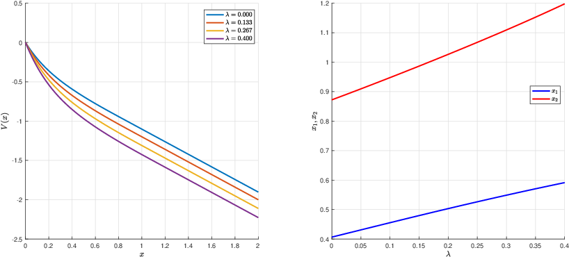
Refer to caption
Fig. 7: The impacts of λ\lambda on the equilibrium value function VV (left panel) and thresholds x1,x2x_{1},x_{2} (right panel).

In Fig. 7, we study the impact of the parameter λ\lambda on the equilibrium value function VV and thresholds x1,x2x_{1},x_{2} given that the other parameters are set to their baseline values. The left panel of Fig. 7 studies the equilibrium value function with four representative curves corresponding to different values of the parameter λ\lambda. The right panel of Fig. 7 examines that how thresholds x1,x2x_{1},x_{2} are varying with respect to λ\lambda. As λ\lambda increases, the discount function increases, resulting in a smaller equilibrium value function. The effort and dividend thresholds x1,x2x_{1},x_{2} are increasing in λ\lambda. The reason is that the larger λ\lambda, the less the discount is applied to future cashflows, and hence, the thresholds for both effort and dividend are raised to reduce the ruin probability to seek for more potential dividends in the future. Specially, the case with λ=0\lambda=0 is time consistent counterpart.

7 Conclusions

In this paper, we investigate a time-inconsistent mixed regular-singular control problem in continuous time under non-exponential discounting and propose a comprehensive equilibrium framework to address the inherent dynamic inconsistency. At the theoretical level, we seek time-consistent equilibria in an intrapersonal game setting and introduce a novel definition of equilibrium regular-singular control law tailored to this class of problems for which the perturbations of regular and singular control are simultaneous, and establish a verification theorem that provides a sufficient condition for the equilibrium. An extended HJB system is derived with verification theorem. In addition, for the case where perturbations are applied separately to the regular and singular control, we propose the concept of mild equilibrium regular-singular control law, together with its corresponding mild verification theorem. These theoretical results extend the existing literature on time-inconsistent control by accommodating both regular and singular components within a unified framework. At the applied level, we demonstrate the practical relevance of our theory through the effort and dividend problem. By solving the extended HJB system, we derive an explicit equilibrium characterized by the effort and dividend thresholds under two representative discount structures: a mixture of exponential discount functions and a pseudo-exponential discount function. The convexity of the value function is rigorously established, and the equilibrium conditions are confirmed. Furthermore, we demonstrate the existence of the effort and dividend thresholds under a mixture of exponential discount functions. Under mild conditions, the equilibrium policy prescribes exerting the maximal level of effort when the surplus falls below the effort threshold and paying dividends once the surplus exceeds the dividend threshold when the cost for dividend is relatively small; otherwise, when the cost for dividend is relatively large, the equilibrium policy is to pay the dividend once the surplus exceeds the dividend threshold and not to apply effort even if the firm is at the ruin time. The closed-form solutions validate the feasibility of our theoretical framework and provides economically intuitive insights for dynamic corporate finance decisions involving effort allocation and shareholder payouts. Numerical analysis further quantifies the effects of key exogenous parameters on the thresholds and the equilibrium value function under the pseudo-exponential discount function, thereby shedding light on their economic implications.

Acknowledgements.

The work is supported by the National Natural Science Foundation of China (12271290, 11871036). The authors thank the members of the group of Mathematical Finance and Actuarial Science at the Department of Mathematical Sciences, Tsinghua University, for their helpful feedback and conversations.

Declaration of generative AI and AI-assisted technologies in the writing process.

During the preparation of this work, the authors used ChatGPT (OpenAI) in order to enhance the clarity and readability of the manuscript. After using this tool, the authors reviewed and edited the content as needed and take full responsibility for the content of the published article.

References

  • Bajeux-Besnainou and Portait (1998) I. Bajeux-Besnainou and R. Portait Dynamic asset allocation in a mean-variance framework. Management Science 44 (11), pp. S79–S95. Cited by: §1.
  • Björk et al. (2017) T. Björk, M. Khapko, and A. Murgoci On time-inconsistent stochastic control in continuous time. Finance and Stochastics 21, pp. 331–360. Cited by: §1, Remark 2.7, §2.
  • Björk et al. (2021) T. Björk, M. Khapko, and A. Murgoci Time-inconsistent control theory with finance applications. First edition, Springer. Cited by: Remark 2.7, §2.
  • Björk et al. (2014) T. Björk, A. Murgoci, and X. Y. Zhou Mean–variance portfolio optimization with state-dependent risk aversion. Mathematical Finance 24 (1), pp. 1–24. Cited by: §1.
  • Björk and Murgoci (2010) T. Björk and A. Murgoci A general theory of markovian time inconsistent stochastic control problems. Available at SSRN 1694759. Cited by: §1.
  • Bodnariu et al. (2025) A. Bodnariu, K. Lindensjö, and N. Rodosthenous Time-inconsistent singular control problems: reflection and absolutely continuous controls with exploding rates. External Links: 2507.04836, Link Cited by: §1.
  • Cadenzas et al. (2007) A. Cadenzas, J. Cvitanić, and F. Zapatero Optimal risk-sharing with effort and project choice. Journal of Economic Theory 133 (1), pp. 403–440. Cited by: §5.1.
  • Cao et al. (2025) J. Cao, D. Li, V. R. Young, and B. Zou Short communication: equilibrium mean-variance dividend rate strategies. SIAM Journal on Financial Mathematics 16 (3), pp. SC64–SC75. Cited by: §1.
  • Cao et al. (2026a) J. Cao, D. Li, V. R. Young, and B. Zou Equilibrium strategies for singular dividend control problems under the mean-variance criterion. SIAM Journal on Control and Optimization 64 (3), pp. 1383–1405. Cited by: §1, Remark 2.5.
  • Cao et al. (2026b) Y. Cao, G. Guan, Z. Liang, and X. Luo Equilibrium singular dividend control under ambiguity aggregation of heterogeneous discount rates. arXiv preprint arXiv:2606.25461. Cited by: §1.
  • Chen et al. (2021) X. Chen, C. Guan, and F. Yi A free boundary problem of liquidity management for optimal dividend and insurance in finite horizon. SIAM Journal on Control and Optimization 59 (4), pp. 2524–2545. Cited by: §1.
  • Christensen and Lindensjö (2018) S. Christensen and K. Lindensjö On finding equilibrium stopping times for time-inconsistent markovian problems. SIAM Journal on Control and Optimization 56 (6), pp. 4228–4255. Cited by: §1.
  • Christensen and Lindensjö (2020) S. Christensen and K. Lindensjö On time-inconsistent stopping problems and mixed strategy stopping times. Stochastic Processes and their Applications 130 (5), pp. 2886–2917. Cited by: §1.
  • Dai et al. (2024) M. Dai, Y. Jia, and H. Jin Dynamic mean-variance portfolio selection with transaction costs. Available at SSRN 4958481. Cited by: §1.
  • Dai et al. (2026) R. Dai, G. Guan, Z. Liang, and X. Luo Time-inconsistent singular control problems with a running minimum process. External Links: 2605.19914, Link Cited by: §1.
  • Dong and Sircar (2014) Y. Dong and R. Sircar Time-inconsistent portfolio investment problems. In Stochastic Analysis and Applications 2014, D. Crisan, B. Hambly, and T. Zariphopoulou (Eds.), Cham, pp. 239–281. Cited by: §1.
  • Ebert et al. (2020) S. Ebert, W. Wei, and X. Y. Zhou Weighted discounting—on group diversity, time-inconsistency, and consequences for investment. Journal of Economic Theory 189, pp. 105089. Cited by: §1, §5.2.
  • Ekeland and Lazrak (2006) I. Ekeland and A. Lazrak Being serious about non-commitment: subgame perfect equilibrium in continuous time. External Links: math/0604264, Link Cited by: §1.
  • Ekeland and Lazrak (2010) I. Ekeland and A. Lazrak The golden rule when preferences are time inconsistent. Mathematics and Financial Economics 4, pp. 29–55. Cited by: §1.
  • Ekeland et al. (2012) I. Ekeland, O. Mbodji, and T. A. Pirvu Time-consistent portfolio management. SIAM Journal on Financial Mathematics 3 (1), pp. 1–32. Cited by: §1.
  • Ekeland and Pirvu (2008) I. Ekeland and T. A. Pirvu Investment and consumption without commitment. Mathematics and Financial Economics 2, pp. 57–86. Cited by: §1, §1, §5.3.
  • Guan et al. (2023) C. Guan, Z. Q. Xu, and R. Zhou Dynamic optimal reinsurance and dividend payout in finite time horizon. Mathematics of Operations Research 48 (1), pp. 544–568. Cited by: §1.
  • Guo et al. (2004) X. Guo, J. Liu, and X. Y. Zhou A constrained non-linear regular-singular stochastic control problem, with applications. Stochastic Processes and their Applications 109 (2), pp. 167–187. Cited by: §1.
  • Harris and Laibson (2001) C. Harris and D. Laibson Dynamic choices of hyperbolic consumers. Econometrica: Journal of the Econometric Society 69 (4), pp. 935–957. Cited by: §1.
  • Hu and Zhou (2025) S. Hu and Z. Zhou Equilibrium policy on dividend and capital injection under time-inconsistent preferences. External Links: 2505.23511, Link Cited by: §1, §5.2, §5.2, §6, §6.
  • Hu et al. (2012) Y. Hu, H. Jin, and X. Y. Zhou Time-inconsistent stochastic linear–quadratic control. SIAM Journal on Control and Optimization 50 (3), pp. 1548–1572. Cited by: §1.
  • Hu et al. (2017) Y. Hu, H. Jin, and X. Y. Zhou Time-inconsistent stochastic linear-quadratic control: characterization and uniqueness of equilibrium. SIAM Journal on Control and Optimization 55 (2), pp. 1261–1279. Cited by: §1.
  • Jgaard and Taksar (1999) B. H. Jgaard and M. Taksar Controlling risk exposure and dividends payout schemes: insurance company example. Mathematical Finance 9 (2), pp. 153–182. Cited by: §1, §1.
  • Kryger and Steffensen (2010) E. M. Kryger and M. Steffensen Some solvable portfolio problems with quadratic and collective objectives. Available at SSRN 1577265. Cited by: §1.
  • Li et al. (2015) D. Li, R. Ximin, and Z. Hui Time-consistent reinsurance–investment strategy for a mean–variance insurer under stochastic interest rate model and inflation risk. Insurance: Mathematics and Economics 64, pp. 28–44. Cited by: §1.
  • Li and Ng (2000) D. Li and W. Ng Optimal dynamic portfolio selection: multiperiod mean-variance formulation. Mathematical Finance 10 (3), pp. 387–406. Cited by: §1.
  • Li et al. (2016) Y. Li, Z. Li, and Y. Zeng Equilibrium dividend strategy with non-exponential discounting in a dual model. Journal of Optimization Theory and Applications 168, pp. 699–722. Cited by: §1.
  • Liang and Young (2026) X. Liang and V. R. Young Time-consistent annuitization and asset allocation under the mean-variance criterion. Journal of Applied Probability 63 (2), pp. 648–667. Cited by: §1.
  • Liang et al. (2024) Z. Liang, X. Luo, and F. Yuan Equilibria for time-inconsistent singular control problems. SIAM Journal on Control and Optimization 62 (6), pp. 3213–3238. Cited by: §1, §1, Remark 2.7, §2.
  • Liang et al. (2026) Z. Liang, X. Luo, and J. Zhang Equilibrium for regular-singular control under mean-variance criterion: a unified approach via control laws. External Links: 2607.26635, Link Cited by: §1.
  • Liang and Luo (2025) Z. Liang and X. Luo Stackelberg reinsurance and premium decisions with mv criterion and irreversibility. SIAM Journal on Financial Mathematics 16 (1), pp. 167–199. Cited by: §1, Remark 2.3, Remark 2.7, §2.
  • Liang and Song (2015) Z. Liang and M. Song Time-consistent reinsurance and investment strategies for mean–variance insurer under partial information. Insurance: Mathematics and Economics 65, pp. 66–76. Cited by: §1.
  • Liang and Yuan (2023) Z. Liang and F. Yuan Weak equilibria for time-inconsistent control: with applications to investment-withdrawal decisions. Mathematical Finance 33 (3), pp. 891–945. Cited by: §1, §1, Remark 2.8, §4.
  • Lin and Qian (2016) X. Lin and Y. Qian Time-consistent mean-variance reinsurance-investment strategy for insurers under cev model. Scandinavian Actuarial Journal 2016 (7), pp. 646–671. Cited by: §1.
  • Marín-Solano and Navas (2010) J. Marín-Solano and J. Navas Consumption and portfolio rules for time-inconsistent investors. European Journal of Operational Research 201 (3), pp. 860–872. Cited by: §1.
  • Peskir (2007) G. Peskir A change-of-variable formula with local time on surfaces. In Séminaire de probabilités XL, pp. 70–96. Cited by: Remark 5.11, Remark 5.3.
  • Qiu et al. (2023) M. Qiu, Z. Jin, and S. Li Optimal risk sharing and dividend strategies under default contagion: a semi-analytical approach. Insurance: Mathematics and Economics 113, pp. 1–23. Cited by: §1.
  • Richardson (1989) H. R. Richardson A minimum variance result in continuous trading portfolio optimization. Management Science 35 (9), pp. 1045–1055. Cited by: §1.
  • Samuelson (1937) P. A. Samuelson A note on measurement of utility. The Review of Economic Studies 4 (2), pp. 155–161. Cited by: §1.
  • Shreve et al. (1984) S. E. Shreve, J. P. Lehoczky, and D. P. Gaver Optimal consumption for general diffusions with absorbing and reflecting barriers. SIAM Journal on Control and Optimization 22 (1), pp. 55–75. Cited by: §5.2, §5.3.
  • Strotz (1955) R. H. Strotz Myopia and inconsistency in dynamic utility maximization. The Review of Economic Studies 23 (3), pp. 165–180. Cited by: §1, §1.
  • Taksar and Zhou (1998) M. I. Taksar and X. Y. Zhou Optimal risk and dividend control for a company with debt liability. Insurance: Mathematics and Economics 22 (1), pp. 105–122. Cited by: §1.
  • Zhang (1994) T. Zhang On the strong solutions of one-dimensional stochastic differential equations with reflecting boundary. Stochastic Processes and their Applications 50 (1), pp. 135–147. Cited by: §5.2.
  • Zhao et al. (2014) Q. Zhao, J. Wei, and R. Wang On dividend strategies with non-exponential discounting. Insurance: Mathematics and Economics 58, pp. 1–13. Cited by: §1, §5.3, §6.
  • Zhou and Li (2000) X. Y. Zhou and D. Li Continuous-time mean-variance portfolio selection: a stochastic lq framework. Applied Mathematics and Optimization 42, pp. 19–33. Cited by: §1.