Scaling-Enhanced Rapid Readout of a Qubit Ensemble Assisted by
High-Frequency Detector Modes

Quantum readout is a fundamental task in quantum science and technology [23, 24, 10]. It converts information stored in quantum degrees of freedom into an accessible classical record and thereby underlies quantum computation, quantum repeaters, and quantum thermodynamics [14, 37, 40, 11, 33, 4]. Ensemble measurements on qubits are particularly important in quantum sensing [17, 18, 47], electron spin resonance (ESR) [1], nuclear magnetic resonance (NMR) [3, 25], and quantum feedback control [12].

In many architectures, the relevant information encoded in a qubit ensemble is not obtained via direct measurement of the qubit ensemble. Instead, a collective observable of the ensemble is coupled to a probe, meter, or output field, which is subsequently measured [21, 49, 8, 30, 13]. For many applications, the information must also be extracted rapidly [15, 22, 7]. If the time required for the indirect readout, which we call readout time, is too long, it increases exposure to unwanted noise, delays feedback operations, and limits the repetition rate of the protocols. Substantial effort has been devoted to improving detectors, amplifiers, and readout resonators on specific platforms for rapid readout [45, 20, 43, 27, 41].

Despite extensive progress in quantum readout, a general principle governing how rapidly information can be transferred from a large qubit ensemble to a detector has not been established. In particular, the scaling of the readout time with the number of qubits $N$ in the ensemble remains unclear. In many studies, the system-size scaling provides a fundamental measure of performance and underlies quantum advantages in quantum metrology, quantum batteries and quantum heat engines [26, 16, 34, 9, 5, 6, 29]. This raises the questions of whether a general scaling benchmark exists for collective readout and whether and how the scaling itself can be improved.

In this Letter, we address this question and show that unbounded high-frequency detector modes can provide a scaling advantage in collective readout. We quantify the information transferred from the qubit ensemble to the detector by their quantum mutual information, which characterize the correlation between the qubit ensemble and the detector. We first establish a lower bound on the readout time as $N^{-1/2}$ for detectors without ultraviolet high-frequency modes. We then propose a new protocol that achieves a more favorable scaling by going beyond the $N^{-1/2}$ benchmark, using unbounded high-frequency detector modes. In the idealized unbounded-frequency limit, the high-frequency modes make the coefficient appearing in the scaling law divergent, and the $N^{-1/2}$ benchmark no longer applies. This leads to a different scaling law $N^{-1/(2-\nu)}$ for $0<\nu<2$, where $\nu$ characterizes the high-frequency behavior of the detector spectral structure. The resulting scaling is parametrically faster than the $N^{-1/2}$ scaling.

Concretely, we consider a spin-boson model in which a product state of $N$ qubits is collectively and longitudinally coupled to a bosonic detector [31, 46, 36]. The qubit information is transferred to the detector through the collective spin-boson interaction. We furthermore investigate a concrete readout protocol in which information about an unknown magnetic field is encoded in the qubit ensemble and the field is estimated by reading out the bosonic detector. We show that the time required to attain the standard quantum limit (SQL), which is characterized by a estimation error of order $N^{-1/2}$, has the same $N$-dependence on time as the mutual-information timescale.

We also show that even when the detector has an ultraviolet cutoff, the scaling advantage persists over a finite range of system sizes. The cutoff determines the range of system sizes over which the enhanced scaling can be observed. Thus, the detector spectrum governs both the attainable scaling of the readout time and the range of system sizes over which this scaling advantage can be realized. Our results identify high-frequency detector modes as a resource for accelerating collective quantum readout.

We here derive a broadly applicable benchmark for the time-scaling required to transfer information from the qubit ensemble to a detector without high-frequency modes. In an indirect measurement, the interaction between the qubit ensemble and the detector generates correlations through which information about the ensemble is transferred to the detector. We quantify this information transfer by the quantum mutual information between the qubit ensemble and the detector, and derive a lower bound on the time-scaling required to generate a fixed amount of such correlation.

For a regular detector, we first obtain the expected timescale $t\sim N^{-1/2}$ using a simple argument and then prove that it gives a rigorous lower bound on the readout time. Throughout this paper, we use units with $\hbar=1$. Suppose that the qubits couple to a detector through an additive observable of the qubit ensemble,

where $O_{\rm S}=\sum_{j=1}^{N}o_{j}$, $[H_{\rm S},O_{\rm S}]=0$, $H$ is the total Hamiltonian, $H_{\rm S}$ is the free Hamiltonian of the qubit ensemble, $g$ is a real constant, $B$ is a Hermitian operator acting on the detector, $H_{\rm D}$ is the free Hamiltonian of the detector, $o_{j}$ is the $N$-independent operator acting on the $j$-th qubit, and $I_{\rm S}$ and $I_{\rm D}$ are the identity operators on the qubit ensemble and detector, respectively. The condition $[H_{\rm S},O_{\rm S}]=0$ implies $[O_{\rm S}\otimes I_{\rm D},H]=0$, so that $O_{\rm S}$ satisfies the quantum-nondemolition (QND) condition. The spectral decomposition of $O_{\rm S}$ is given by $O_{\rm S}=\sum_{m}mP_{m}$, where $P_{m}$ is the projection operator onto the eigenspace of $O_{\rm S}$ with eigenvalue $m$. We prepare an initial state as $\ket{\psi(0)}=\ket{s_{0}}\otimes\ket{d_{0}}$. The state at time $t$ is given by

where $p_{m}:=\braket{s_{0}|P_{m}|s_{0}}$, $\ket{s_{m}}:=P_{m}\ket{s_{0}}/\sqrt{p_{m}}$, $\ket{s_{m}(t)}:=\mathrm{e}^{-\mathrm{i}H_{\rm S}t}\ket{s_{m}}$, and $\ket{d_{m}(t)}:=\mathrm{e}^{-\mathrm{i}(H_{\rm D}+gmB)t}\ket{d_{0}}$.

We first give a simple argument for the timescale for generating correlations between the qubit ensemble and the detector [48]. For an initially pure product state, the short-time entanglement generation induced by the product interaction $gO_{\rm S}\otimes B$ is governed by the fluctuations of the two coupling operators: the characteristic scale governing the initial generation of entanglement [48] is $|g|\Delta O_{\rm S}\Delta B$, where $\Delta^{2}O_{\rm S}:=\braket{s_{0}|O_{\rm S}^{2}|s_{0}}-\braket{s_{0}|O_{\rm S}|s_{0}}^{2}$ and $\Delta^{2}B:=\braket{d_{0}|B^{2}|d_{0}}-\braket{d_{0}|B|d_{0}}^{2}$. This quantity characterizes the strength with which the interaction generates correlations from the initial product state and has the dimension of an inverse time. We therefore set the characteristic timescale as its inverse given by $(|g|\Delta O_{\rm S}\Delta B)^{-1}$. When we assume a pure product input state $\ket{s_{0}}=\bigotimes_{j=1}^{N}\ket{\psi_{j}}$ and assume that the average local fluctuation remains finite and nonzero, the variance of the additive observable scales as $\Delta^{2}O_{\rm S}=\Theta(N)$. Therefore, when $g$ and $\Delta^{2}B$ are finite and independent of $N$, the timescale of generating correlations is $\Theta(N^{-1/2})$. Thus, the characteristic timescale is expected to scale as $t\sim N^{-1/2}$ for generating correlations between the qubit ensemble and the detector.

We then show that the same $N^{-1/2}$ scaling gives a rigorous lower bound on the readout time by quantifying the quantum mutual information, which is an measure of the total correlation between the qubit ensemble and the detector generated by their interaction. Since the total state is pure, the quantum mutual information is twice the entanglement entropy as $I_{\rm S:D}(t)=2S(\rho_{\rm D}(t))$, where $S(\rho):=-\Tr[\rho\log\rho]$ is the von Neumann entropy, $\rho_{\rm S}(t):=\Tr_{\rm D}[\outerproduct{\psi(t)}{\psi(t)}]$ is the qubit state, and $\rho_{\rm D}(t):=\Tr_{\rm S}[\outerproduct{\psi(t)}{\psi(t)}]$ is the detector state.

Whenever the maximum variance of $B$ under the conditional detector state $\ket{d_{m}(s)}$ defined as $V_{\rm B}:=\sup_{m,s\geq 0}\operatorname{Var}_{\ket{d_{m}(s)}}(B)$ is finite and independent of $N$, the quantum mutual information is bounded from above as follows:

where $t_{\rm corr}:=\inf\{t>0:I_{\rm S:D}(t)\geq I_{0}\}$, $I_{0}>0$ and $C$ are independent of $N$ and $t$, respectively [44]. The correlation time defined above $t_{\rm corr}$ quantifies the time needed to generate a constant amount of correlation between the qubit ensemble and the detector for the quantum mutual information.

Therefore, we obtain the readout-time bound $t_{\rm corr}=\Omega(N^{-1/2})$ whenever $V_{\rm B}$ remains finite. The finiteness of $V_{\rm B}$ bounds the fluctuations of the detector coupling operator along all conditional detector states. High-frequency detector modes can violate this condition due to the divergent of $V_{\rm B}$, for which Eq. (3) no longer gives a nonzero lower bound on $t_{\rm corr}$. We next determine the resulting readout timescale explicitly for a bosonic detector with such unbounded high-frequency modes.

The $N^{-1/2}$ lower bound derived above is applicable for a broad class, but its discussion is based on a finite coefficient $V_{\rm B}$. However, if we exploit unbounded high-frequency detector modes, $V_{\rm B}$ may diverge and the bound derived in Eq. (3) no longer applies. We now propose a protocol to achieve a scaling advantage in the readout time in this case. Concretely, we consider the bosonic detector with a ultraviolet component [31, 46, 36] and evaluate the lower and upper bounds on the quantum mutual information. We show that both the lower and upper bounds are functions of $Nt^{2-\nu}$ for $0<\nu<2$, which leads to the characteristic time scaling $t_{\rm corr}=\Theta(N^{-1/(2-\nu)})$.

Let us specialize Eq. (1) to a bosonic detector consisting of a set of modes as follows:

which satisfies the QND condition $\quantity[H_{\rm S},O_{\rm S}]=0$. Here, $b_{k}$ annihilates an excitation in detector mode $k$ of angular frequency $\omega_{k}$, and the parameter $g_{k}$ is the real coupling strength to mode $k$. As discussed in Eq. (1), the spectral decomposition of $O_{\rm S}$ is given by $O_{\rm S}=\sum_{m}mP_{m}$. We prepare the detector in the vacuum and the qubits in the initial pure state $\ket{\phi(0)}=\ket{s_{0}}\otimes\ket{\rm vac}_{\rm D}.$

By using the above setting, we obtain the reduced state of the detector in the interaction picture as follows:

where $p_{m}=\braket{s_{0}|P_{m}|s_{0}}$ and $\alpha_{k}(t):=(1-\mathrm{e}^{\mathrm{i}\omega_{k}t})/\omega_{k}$ [44]. Note that since the picture transformation is a local unitary operation, the quantum mutual information is invariant under the picture transformation. The conditional coherent state $\ket{\beta_{m}(t)}_{\rm D}$ satisfies the following inner product:

We then derive bounds on the quantum mutual information $I_{\rm S:D}(t)$ for the product input $\ket{s_{0}}=\bigotimes_{j=1}^{N}\ket{\psi_{j}}$ and the additive observable $O_{\rm S}=\sum_{j=1}^{N}o_{j}$, where $o_{j}$ is independent of $N$. Using the second Rényi entropy for the lower bound and the positivity of the quantum relative entropy for the upper bound, we obtain the following bounds on the quantum mutual information derived in the End Matter:

For $A(t)\Delta^{2}O_{\rm S}\to 0$, the upper bound vanishes, and finite amount of qubits–detector correlation cannot be generated. On the other hand, for $A(t)\Delta^{2}O_{\rm S}=X_{0}$ with a fixed value $X_{0}$, both the lower and upper bound remains finite and positive in the large-$N$ limit. Therefore, for the product input with $\Delta^{2}O_{\rm S}=\Theta(N)$, the characteristic correlation-formation scale is $A(t)\Delta^{2}O_{\rm S}=\Theta(1)$, or equivalently $A(t)N=\Theta(1)$.

We then evaluate the behavior of $A(t)$. Assume the dispersion relation $\omega(\vec{k})=\Omega|\vec{k}|^{n}$ with $\Omega>0$ in $D$ spatial dimensions and a constant coupling $g$. Here, starting from the finite discrete-mode model, we take the continuum and infinite-cutoff limits to model an ideal detector with unbounded high-frequency modes as follows:

where $S_{D}:=2\pi^{D/2}/\Gamma(D/2)$ is the surface area of a unit sphere in $D$ dimensions with $\Gamma(\cdot)$ being the gamma function, and $S_{D}k^{D-1}\differential k$ is the radial integration measure. For $\nu:=D/n$ with $0<\nu<2$, changing the integration variable to $u:=\Omega k^{n}t$, we obtain the fractional behavior [35] of $A(t)$ as follows:

where $C_{\nu}={\pi S_{D}/(n\Gamma(3-\nu)\sin(\pi\nu/2))}$. Substituting Eq. (10) into $A(t)\Delta^{2}O_{\rm S}=\Theta(1)$ and using $\Delta^{2}O_{\rm S}=\Theta(N)$, we find that the characteristic readout timescale is therefore $t_{\rm corr}=\Theta\left(N^{-1/(2-\nu)}\right).$ Since $1/(2-\nu)>1/2$, this time is shorter than the conventional timescale $\Theta(N^{-1/2})$. The scaling advantage originates from the behavior of $A(t)$, rather than from a change in the qubit fluctuations. For a regular detector with $V_{\rm B}<\infty$, $A(t)\propto t^{2}$, which yields the $N^{-1/2}$ timescale. On the other hand, unbounded high-frequency modes give $A(t)\propto t^{2-\nu}$, leading to $N^{-1/(2-\nu)}$. The high-frequency spectral structure changes the exponent of the system-size scaling itself.

The mutual-information analysis above establishes the scaling of the time required to generate correlations between the qubit ensemble and the detector. We now give an operational example based on the magnetic field estimation. First, information about an unknown magnetic field $\omega_{0}$ is encoded in the spin state through its interaction with the spin ensemble. The ensemble is then coupled to a bosonic detector, after which the photon number of an appropriately chosen detector mode is measured to estimate the magnetic field. We show that, in this protocol, the time required to attain SQL sensitivity within a fixed constant factor has the same $N$-dependence as the mutual-information criterion discussed above.

Let us take the spin ensemble state encoded with the unknown parameter $\theta:=\omega_{0}\tau$, where $\tau$ is the interrogation time, and the vacuum state of the detector as the initial state:

We set the additive observable $O_{\rm S}=J_{z}:=\sum_{j=1}^{N}\sigma_{z}^{(j)}$ in Eq. (4), with $\sigma_{z}\ket{1}=\ket{1}$ and $\sigma_{z}\ket{0}=-\ket{0}$. The eigenvalue $m=2\ell-N$ occurs with the binomial probability $q_{\ell}$, where $\ell$ is the number of qubits in $\ket{1}$.

The reduced detector state at time $t$ in the interaction picture is

The coefficient $q_{\ell}$ is the binomial probability of obtaining $\ell$ qubits in $\ket{1}_{\mathrm{S}}$.

We then introduce the collective detector mode

and consider the photon-number measurement of this mode $\mathcal{N}(t):=B_{0}^{\dagger}(t)B_{0}(t)$. The expectation value of the photon number operator is $\braket{\mathcal{N}(t)}:=\Tr_{\rm D}\quantity[\rho_{\rm D}^{\rm I}(t)\mathcal{N}(t)]$.

We quantify the error for estimating $\theta$ given by $\Delta^{2}\theta:=\Delta^{2}\mathcal{N}(t)/\partial_{\theta}\absolutevalue{\partial_{\theta}\braket{\mathcal{N}(t)}}^{2}$, where $\Delta^{2}\mathcal{N}(t):=\braket{\mathcal{N}^{2}(t)}-\braket{\mathcal{N}(t)}^{2}$ is the variance of the photon number operator. Using the exact photon-number moments and the corresponding finite-$N$ expression, we obtain the following result for large $N$ [44]:

Note that we assume that $\sin(4\theta)\neq 0$ to avoid the divergence. The first term in Eq. (14) gives the SQL contribution $1/(4N)$, whereas the finite readout time produces the second term proportional to $1/[A(t)N^{2}]$. The latter becomes of order $1/N$ when $A(t)N=\Theta(1)$. Thus, the photon-number measurement reaches SQL precision on the same characteristic timescale obtained above from the quantum mutual information. More precisely, defining $t_{\rm SQL}:=\inf\{t>0:\Delta^{2}\theta(t)\leq c/N\}$ with a constant $c>1/4$, Eq. (14) requires $A(t_{\rm SQL})=\Theta(N^{-1})$.

For a regular detector with the conventional quadratic response $A(t)\propto t^{2}$, this condition gives $t_{\rm SQL}=\Theta(N^{-1/2}).$ By contrast, for the unbounded high-frequency detector considered here, $A(t)\propto t^{2-\nu}$ from Eq. (10), and hence $t_{\rm SQL}=\Theta\left(N^{-1/(2-\nu)}\right).$ Thus, for the same readout protocol and the same SQL-precision criterion, the high-frequency detector changes the scaling of the required measurement time from $N^{-1/2}$ to $N^{-1/(2-\nu)}$.

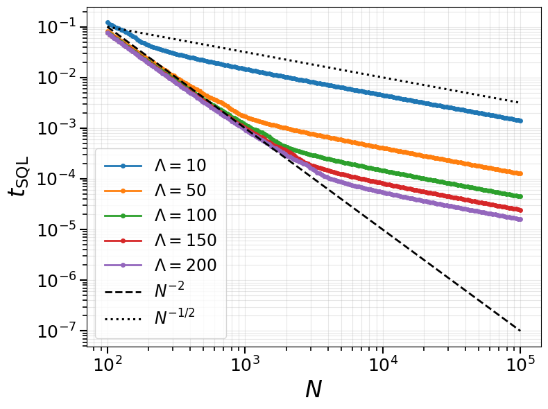
The above analysis assumes an idealized infinite frequency range of the detector. In practice, the detector has a finite bandwidth, which can be modeled by an ultraviolet wave-number cutoff $\Lambda$. However, in the presence of a finite cutoff, the same scaling of the readout time is still observed for a finite range of $N$. Let us introduce the ultraviolet cutoff $\Lambda$ in Eq. (9), i.e., truncate the integral at $\Lambda$. Even with this cutoff, for times $t\gg(\Omega\Lambda^{n})^{-1}$, the fractional behavior $A(t)\simeq C_{\nu}|g|^{2}t^{2-\nu}/\Omega^{\nu}$ in Eq. (10) is still valid [44]. Therefore, the enhanced scaling $N^{-1/(2-\nu)}$ is observed if the enhanced scaling time is longer than the ultraviolet timescale, i.e., $t_{\rm corr},~t_{\rm SQL}\gg(\Omega\Lambda^{n})^{-1}$. Since the characteristic readout time scales as

up to a constant factor, this condition gives

Equivalently, for a fixed cutoff $\Lambda$, the enhanced scaling is observed for $N\ll N_{\rm c}$ with $N_{\rm c}\sim\Omega^{2}\Lambda^{n(2-\nu)}/(C_{\nu}|g|^{2})$, see Fig. 1. On the other hand, for $N\gg N_{\rm c}$, since $A(t)$ behaves as a quadratic function of time in the relevant time regime, the scaling of the readout time returns to the conventional $N^{-1/2}$ scaling.

For a finite cutoff, the exponent $\nu$ determines the enhanced system-size scaling, whereas the cutoff $\Lambda$ determines the range of $N$ over which this scaling can be observed. Increasing $\Lambda$ therefore shifts the crossover $N_{\rm c}$ toward larger system sizes, while the asymptotic behavior at fixed finite $\Lambda$ eventually returns to $N^{-1/2}$. In this sense, high-frequency modes control the range of system sizes over which the readout advantage is accessible. Thus, the cutoff serves as a resource for rapid readout of a finite number of qubits.

We first established a lower bound on the readout time of a qubit ensemble by quantifying the quantum mutual information between the qubit ensemble and the detector. The lower bound is given by $t_{\rm corr}=\Omega(N^{-1/2})$ and is applicable to a broad class of detectors without ultraviolet high-frequency modes. We then showed that high-frequency detector modes can accelerate collective readout to $t_{\rm corr}\propto N^{-1/(2-\nu)}$ with $0<\nu<2$. These results establish high-frequency spectral structure as a resource for accelerating collective readout and suggest spectral engineering of detectors as a route toward fast measurement of large quantum ensembles. The same accelerated scaling is attained by the photon-number readout and persists over a finite range of system sizes in the presence of a finite detector cutoff.

References

- [1] (2016) Reaching the quantum limit of sensitivity in electron spin resonance. Nature Nanotechnology 11 (3), pp. 253–257. Cited by: Introduction.—.
- [2] (2009) The Magnus expansion and some of its applications. Physics Reports 470 (5–6), pp. 151–238. External Links: Document Cited by: §II.
- [3] (1946) The nuclear induction experiment. Physical Review 70 (7-8), pp. 474. Cited by: Introduction.—.
- [4] (1998) Quantum repeaters: The role of imperfect local operations in quantum communication. Physical Review Letters 81 (26), pp. 5932–5935. External Links: Document Cited by: Introduction.—.
- [5] (2017) Enhancing the charging power of quantum batteries. Physical Review Letters 118 (15), pp. 150601. External Links: Document Cited by: Introduction.—.
- [6] (2016) The power of a critical heat engine. Nature Communications 7 (1), pp. 11895. External Links: Document Cited by: Introduction.—.
- [7] (2023) Transmon qubit readout fidelity at the threshold for quantum error correction without a quantum-limited amplifier. npj Quantum Information 9 (1), pp. 26. Cited by: Introduction.—.
- [8] (2014) Cavity-aided nondemolition measurements for atom counting and spin squeezing. Physical Review A 89 (4), pp. 043837. Cited by: Introduction.—.
- [9] (2012) Quantum metrology in non-Markovian environments. Physical Review Letters 109 (23), pp. 233601. External Links: Document Cited by: Introduction.—.
- [10] (2010) Introduction to quantum noise, measurement, and amplification. Reviews of Modern Physics 82 (2), pp. 1155–1208. Cited by: Introduction.—.
- [11] (2017) Observing a quantum Maxwell demon at work. Proceedings of the National Academy of Sciences 114 (29), pp. 7561–7564. Cited by: Introduction.—.
- [12] (2016) Deterministic squeezed states with collective measurements and feedback. Physical Review Letters 116 (9), pp. 093602. External Links: Document Cited by: Introduction.—.
- [13] (2021) Cavity-enhanced microwave readout of a solid-state spin sensor. Nature Communications 12 (1), pp. 1357. Cited by: Introduction.—.
- [14] (2004) Single-shot read-out of an individual electron spin in a quantum dot. Nature 430 (6998), pp. 431–435. Cited by: Introduction.—.
- [15] (2012) Surface codes: Towards practical large-scale quantum computation. Physical Review A—Atomic, Molecular, and Optical Physics 86 (3), pp. 032324. Cited by: Introduction.—.
- [16] (2004) Quantum-enhanced measurements: beating the standard quantum limit. Science 306 (5700), pp. 1330–1336. External Links: Document Cited by: Introduction.—.
- [17] (2006) Quantum metrology. Physical Review Letters 96 (1), pp. 010401. External Links: Document Cited by: Introduction.—.
- [18] (2011) Advances in quantum metrology. Nature Photonics 5 (4), pp. 222–229. External Links: Document Cited by: Introduction.—.
- [19] (1963) Coherent and incoherent states of the radiation field. Physical Review 131 (6), pp. 2766–2788. External Links: Document Cited by: §II.
- [20] (2024) Single-shot readout of a superconducting qubit using a thermal detector. Nature Electronics 7 (4), pp. 288–298. Cited by: Introduction.—.
- [21] (2010) Quantum interface between light and atomic ensembles. Reviews of Modern Physics 82 (2), pp. 1041–1093. External Links: Document Cited by: Introduction.—.
- [22] (2018) Rapid high-fidelity multiplexed readout of superconducting qubits. Physical Review Applied 10 (3), pp. 034040. Cited by: Introduction.—.
- [23] (1976) Quantum Detection and Estimation Theory. Academic Press, New York. Cited by: Introduction.—.
- [24] (1982) Probabilistic and Statistical Aspects of Quantum Theory. North-Holland, Amsterdam. Cited by: Introduction.—.
- [25] (1976) The signal-to-noise ratio of the nuclear magnetic resonance experiment. Journal of Magnetic Resonance (1969) 24 (1), pp. 71–85. Cited by: Introduction.—.
- [26] (1997) Improvement of frequency standards with quantum entanglement. Physical Review Letters 79 (20), pp. 3865–3868. External Links: Document Cited by: Introduction.—.
- [27] (2014) Fast accurate state measurement with superconducting qubits. Physical Review Letters 112 (19), pp. 190504. Cited by: Introduction.—.
- [28] (2005) Univariate discrete distributions. 3 edition, Wiley. Cited by: §IV, §IV.
- [29] (2022) Quantum-enhanced heat engine based on superabsorption. Physical Review Letters 128 (18), pp. 180602. External Links: Document Cited by: Introduction.—.
- [30] (2017) Cavity-assisted measurement and coherent control of collective atomic spin oscillators. Physical Review Letters 118 (6), pp. 063604. Cited by: Introduction.—.
- [31] (1987) Dynamics of the dissipative two-state system. Reviews of Modern Physics 59 (1), pp. 1–85. External Links: Document Cited by: Introduction.—, High-frequency enhanced collective readout.—.
- [32] (1995) Optical Coherence and Quantum Optics. Cambridge University Press, Cambridge. Cited by: §II.
- [33] (2018) Information-to-work conversion by Maxwell’s demon in a superconducting circuit quantum electrodynamical system. Nature Communications 9 (1), pp. 1291. Cited by: Introduction.—.
- [34] (2011) Magnetic field sensing beyond the standard quantum limit under the effect of decoherence. Physical Review A 84 (1), pp. 012103. External Links: Document Cited by: Introduction.—.
- [35] (2026) Fractional power-law decay in the spontaneous emission of a two-level system. Physical Review A 114 (2), pp. L020202. External Links: Document Cited by: High-frequency enhanced collective readout.—.
- [36] (1996) Quantum computers and dissipation. Proceedings of the Royal Society of London. Series A: Mathematical, Physical and Engineering Sciences 452 (1946), pp. 567–584. External Links: Document Cited by: Introduction.—, High-frequency enhanced collective readout.—.
- [37] (2013) High-fidelity readout and control of a nuclear spin qubit in silicon. Nature 496 (7445), pp. 334–338. Cited by: Introduction.—.
- [38] (2005) Security of Quantum Key Distribution. Ph.D. Thesis, ETH Zurich. External Links: Document, quant-ph/0512258 Cited by: Lower bound on the quantum mutual information.—.
- [39] (1961) On measures of entropy and information. In Proceedings of the Fourth Berkeley Symposium on Mathematical Statistics and Probability, Vol. 1, Berkeley, California, pp. 547–561. Cited by: Lower bound on the quantum mutual information.—.
- [40] (2008) Second law of thermodynamics with discrete quantum feedback control. Physical Review Letters 100 (8), pp. 080403. Cited by: Introduction.—.
- [41] (2025) Fast multiplexed superconducting-qubit readout with intrinsic purcell filtering using a multiconductor transmission line. PRX Quantum 6 (2), pp. 020345. Cited by: Introduction.—.
- [42] (1963) Equivalence of semiclassical and quantum mechanical descriptions of statistical light beams. Physical Review Letters 10 (7), pp. 277–279. External Links: Document Cited by: §II.
- [43] (2024) Photon-noise-tolerant dispersive readout of a superconducting qubit using a nonlinear Purcell filter. PRX Quantum 5 (1), pp. 010307. Cited by: Introduction.—.
- [44] Note: See the Supplemental Material for details Cited by: General benchmark for collective readout.—, High-frequency enhanced collective readout.—, Photon-number readout and SQL time as a concrete protocol.—, Effect of a finite cutoff.—.
- [45] (2017) Rapid high-fidelity single-shot dispersive readout of superconducting qubits. Physical Review Applied 7 (5), pp. 054020. Cited by: Introduction.—.
- [46] (2012) Quantum Dissipative Systems. 4 edition, World Scientific, Singapore. Cited by: Introduction.—, High-frequency enhanced collective readout.—.
- [47] (1992) Spin squeezing and reduced quantum noise in spectroscopy. Physical Review A 46 (11), pp. R6797–R6800. External Links: Document Cited by: Introduction.—.
- [48] (2018) Entanglement timescale. Physical Review D 97 (6), pp. 066008. Cited by: General benchmark for collective readout.—.
- [49] (2012) Collective state measurement of mesoscopic ensembles with single-atom resolution. Physical Review Letters 109 (13), pp. 133603. Cited by: Introduction.—.