Masking Radar Cognition under Adversarial Surveillance: A Distributional Privacy Framework
Abstract
In this article, we propose an online electronic counter-countermeasure (ECCM) framework designed to conceal the strategic decision-making processes of a cognitive radar (CR) operating under adversarial surveillance. We model the CR under two distinct decision paradigms: a static constrained utility-maximizing behavior and a dynamic expected utility-maximizing behavior. The radar’s utility function is modeled via a von Mises–Fisher (vMF) distribution, with the distributional parameter constituting the private information to be protected from adversarial inference. We adopt a distribution privacy framework to conceal this private information and provide formal distribution privacy guarantees for cognition masking. In this work, we develop cognition-hiding algorithms for both static constrained utility maximization (WDPCH-SU), and dynamic expected utility maximization (WDPCH-DU). Through rigorous mathematical analysis, we show that both WDPCH-SU and WDPCH-DU satisfy -distribution privacy (-DistP) against inference-based adversarial attacks and present the privacy–performance trade-off bounds, quantifying utility loss (in static setting) and expected utility deviation (in dynamic setting) as functions of . Numerical results show that WDPCH-SU gives about 15% improvement in utility loss at maximum privacy compared to the existing methodology while WDPCH-DU achieves a greater reduction in adversarial Fisher information without requiring explicit Fisher information constraints, at a moderate, analytically bounded utility deviation. These results are highly promising in many 6G communication scenarios such as network slicing for automated driving and swarm UAV coordination, where it is essential to keep the resource allocation policy robust against privacy attacks.
Index Terms:
Cognitive radar (CR), electronic warfare, adversarial inference, electronic countermeasure (ECM), electronic counter-countermeasure (ECCM), utility-maximizing behavior, von Mises–Fisher (vMF) distribution, distributional privacy, Wasserstein distance.I Introduction
Traditionally, radar systems operated using predefined search patterns and periodic track updates, with limited ability to adapt to dynamic environments. The emergence of cognitive radar (CR) [1] has transformed this paradigm by incorporating learning and adaptation into the radar decision-making process, allowing the radar to refine its actions based on past observations and perception of the environment. This adaptive capability improves system performance and extends its applicability to complex and uncertain electromagnetic environments [2], optimal waveform selection [3], efficient resource management [4], and robust multi-target tracking [5].
The increasing deployment of CR systems has also accelerated advancements in electronic countermeasures (ECM) [6] and electronic counter-countermeasures (ECCM) [7]. In this paper, we consider an adversarial environment, wherein an intelligent adversary observes the actions of a CR system over time and exploit this observable behavior to estimate the underlying model parameters, consequently deducing the decision-making strategy, a process referred to in this paper as inverse learning. Only a few works in the literature explicitly address ECCM against inverse learning. For example, [8, 9] developed algorithms that reduce the Fisher information available to an adversarial estimator. However, these methods lack formal statistical guarantees to protect the internal decision-making processes of CR systems.
In this work, we address this limitation by formulating the ECCM problem in a distributional privacy setting. The radar is modeled under two complementary paradigms: a static constrained utility-maximizing behavior and a dynamic expected utility-maximizing behavior modelled using a long-run average reward Markov Decision Process (MDP). To the best of our knowledge, ours is the first work to introduce formal distribution privacy guarantees for cognition masking in cognitive radar ECCM. The main contributions of this article are as follows:
- 1.
We develop WDPCH-SU, a cognition-hiding algorithm for a static constrained utility-maximization setting—applicable to single-stage resource allocation tasks such as beam allocation, waveform selection, and power allocation.
- 2.
We develop WDPCH-DU, a cognition-hiding algorithm for dynamic expected utility-maximization over a long-run average reward Markov decision process—applicable to tasks such as operating-mode selection and SINR-based action planning.
- 3.
We prove that both WDPCH-SU and WDPCH-DU satisfy -distribution privacy (-DistP), providing formal guarantees against inference-based adversarial attacks on the radar’s decision-making process.
- 4.
We derive analytical bounds characterizing the privacy–performance trade-off, quantifying utility loss in the static setting and expected utility deviation in the dynamic framework, as a function of the privacy budget .
- 5.
Numerical results demonstrate that WDPCH-SU achieves lower utility loss and stronger privacy than existing methodology [10] for the same privacy budget, while WDPCH-DU achieves a larger reduction in adversarial Fisher information than existing approaches, without requiring explicit Fisher information constraints [9] or transition probability perturbation [11]—both with minimal modifications to baseline radar controllers.
Organization of the article: The remainder of this article is organized as follows. Section II reviews the related literature. Section III introduces the concept of distributional privacy and the theoretical foundations used in this work. Sections IV and V develop the proposed ECCM algorithms, namely WDPCH-SU and WDPCH-DU, respectively. Section VI presents numerical results. Finally, Section VII offers concluding remarks.
II Related Work
The evolution of electronic counter-countermeasures (ECCM) in radar systems reflects a shift from mitigating signal-level interference to safeguarding decision-making processes against adversarial inference. With the emergence of cognitive radar, adversaries increasingly seek to infer internal objectives, state estimates, and decision strategies from observable behavior [12, 1, 13, 4], necessitating ECCM paradigms beyond traditional signal processing techniques.
II-A Classical ECM and ECCM
Classical electronic countermeasures (ECM) degrade radar performance through noise and deceptive jamming, and correspondingly, classical ECCM techniques enhance robustness at the signal level. Representative ECCM approaches include spread-spectrum methods such as Direct Sequence Spread Spectrum (DSSS) and Frequency Hopping Spread Spectrum (FHSS) for mitigating narrowband interference [14, 15], space–time adaptive processing (STAP) for suppressing non-stationary interference [16, 17], and beamforming for spatial interference suppression [18]. However, these methods do not address vulnerabilities arising from inference-based attacks on radar decision processes.
II-B Cognitive Radar: ECM and ECCM
The introduction of cognition into radar systems has led to more sophisticated adversarial strategies, broadly categorized as cognitive jamming and inverse learning. Cognitive jamming exploits radar behavior using learning and optimization frameworks, including game-theoretic formulations for radar–jammer interaction [19, 20], principal–agent models capturing information asymmetry [7], and reinforcement learning-based adaptive jamming strategies [21, 22]. Inverse learning attacks aim to infer an agent’s internal model from observed actions [23, 24], enabling reconstruction of internal state estimates [25, 26] or decision-making policies and objectives [27, 28]. Unlike jamming, inverse learning constitutes a persistent threat by enabling long-term exploitation of radar behavior.
Complementary to these adversarial ECM techniques, ECCM strategies include adaptive sensor selection [29], reinforcement learning-based anti-jamming [30, 31], and adversarial bandit and game-theoretic formulations [32, 33]. While these approaches improve robustness against intelligent interference, they primarily focus on performance optimization and do not explicitly address adversarial inference of radar decision-making policies.
II-C Metacognitive Radar and Masking Strategies
To mitigate inference-based threats, metacognitive radar frameworks have been proposed [10], wherein the radar perturbs its action strategy to obscure underlying objectives and hinder adversarial learning. More broadly, masking of action strategies has been explored across domains via deception and randomized control policies, including KL-divergence-based stealth attacks [34], control-theoretic deception [35], inverse reinforcement learning and revealed preference-based masking [10], entropy-maximizing policies [36], and Fisher information minimization [37]. In the context of radar systems, action-plan masking [8] and Fisher information-based approaches [9] have been investigated, wherein the radar purposefully reduces the determinant of the adversary’s Fisher Information Matrix (FIM) [38, 39, 40, 41] to increase adversarial estimation uncertainty. While effective empirically, none of these approaches—whether heuristic masking, revealed preference-based perturbation, or FIM minimization—provide formal statistical guarantees on what an adversary can infer about the radar’s decision-making parameters. They are further limited by reliance on specific adversarial assumptions and, in the case of FIM-based formulations, non-convex optimization that precludes tractable worst-case analysis.
II-D Privacy Frameworks
Differential privacy (DP) [42, 43] provides a principled framework for limiting information leakage in statistical systems, offering worst-case guarantees on what can be inferred about any individual data point. Distribution privacy [44] extends this notion to the distributional level, protecting the parameters governing the underlying distribution rather than individual records—useful in settings where the data-generating distribution itself is the sensitive quantity. However, conventional distribution privacy mechanisms often incur significant utility loss. The Wasserstein mechanism [45, 46] achieves an improved utility–privacy trade-off while preserving distribution-level guarantees. These frameworks have also been extended to sequential decision-making, with privacy-preserving policy synthesis in MDPs explored in [11].
Existing literature addresses signal-level ECCM, radar–jammer interactions, inverse learning attacks, and heuristic masking strategies, yet a framework for cognition hiding with formal statistical guarantees remains lacking.
III Background: Distribution Privacy and Wasserstein Mechanisms
Distribution privacy provides a principled framework for obfuscating the radar’s cognitive strategy.
Definition III.1 (-Distribution Privacy [46]).
A radar’s decision-making satisfies -distribution privacy if, for any dataset observed by the adversary and any two neighboring parameters and , the likelihood ratio of under the corresponding distributions and satisfies
| (1) |
We refer to this guarantee as -distribution privacy (-DistP).
-DistP guarantees that, with probability at least , an adversary observing cannot reliably distinguish whether it was generated under or , thereby fundamentally limiting its ability to infer the latent cognitive parameter governing the radar’s decision-making process.
Definition III.2 (-Wasserstein Distance).
For two probability distributions and in , let represent the set of all joint distributions with marginals and . The -Wasserstein distance between and is given by:
| (2) |
The -Wasserstein distance focuses on the worst-case cost required to map one distribution to another, making it useful in privacy and robustness scenarios where the most extreme deviations define the system sensitivity. The maximum -Wasserstein distance over a collection of distributions is
| (3) |
IV Masking the Static Utility of a Cognitive Radar

IV-A CR Framework for Static Utility Maximization
In this section, we consider a mathematical framework to model the interaction between a cognitive radar (CR) and an intelligent adversary in an electronic warfare environment. The CR aims to track a target, such as a drone, UAV, or aircraft, while the adversary monitors the radar’s actions to infer the underlying decision-making parameters governing radar behavior. To characterize this interaction, we adopt the widely used Fully Adaptive Radar (FAR) framework [4, 3], shown in Fig. 1 and adapted from [26, 27, 28]. The framework comprises a scene describing the target dynamics, a sensor module, a Bayesian tracker, and a perception-driven radar controller that selects optimal actions by maximizing an associated utility function. Fig. 1 also depicts an adversary equipped with an inverse learner, which observes the radar’s actions to infer the underlying decision-making parameters. As a canonical example, we consider the scenario in Fig. 2, where a cognitive radar tracks multiple targets and allocates its beam resources among them based on their perceived tracking accuracy, while an adversary manipulates target maneuvers and observes the resulting allocations to infer the radar’s cognitive strategy. In the following, we define the various components of the FAR framework.
The scene consists of a moving target whose kinematic state evolves in discrete time, . Let denote the target kinematic state at time . Assuming Markovian dynamics, the state evolves according to
| (4) |
The sensor comprises a transceiver that illuminates the environment and records the reflected signal. The resulting observation is a noisy measurement of the target state , governed by the conditional density
| (5) |
The cognitive radar employs a Bayesian tracker—such as a Kalman filter for linear Gaussian models [1, 13] or a particle filter for nonlinear and non-Gaussian models [47, 48]—to compute a posterior belief over the target state. Let denote the posterior belief at time :
| (6) |
where denotes the accumulated measurement sequence up to time . From this belief, the tracker generates the scene perception vector . For the example in Fig. 2, , whose -th entry
| (7) |
is the predicted tracking accuracy for target [28, 27], where denotes the matrix trace. For instance, under a Kalman filter, the belief is parameterized as , and is the -th diagonal block of the predicted error covariance , with obtained by propagating through the motion dynamics in (4).
Conditioned on the scene perception , the radar controller selects an action, for example beam allocation in Fig. 2, —the response signal—by solving the constrained utility-maximization problem
| (8) | ||||
where is the utility function governing the radar’s relative preference across the targets.

IV-B Adversarial Inverse Learning
Fig. 1 illustrates the proposed inverse learning framework for adversarial cognition inference. At time , the adversary probes the radar through deliberate target maneuvers—such as changes in acceleration—which generate the scene/target state , and observes the resulting radar response . Using and , and assuming the motion dynamics in (4) are known, the adversary’s inverse learner performs inverse filtering [26, 25] to compute the corresponding scene perception vector . Over time, this yields the dataset , consisting of the sequence of recovered perception vectors together with the corresponding radar responses , accumulated over time steps. Based on , the adversary aims to infer the underlying utility function . If exposed, this inferred utility can be exploited by the adversary to design countermeasures that degrade the radar’s tracking performance.
IV-C Stochastic Linear Utility Model
In this paper, we restrict our attention to a linear utility function [28, 27], i.e., . In addition, we assume a stochastic prior for . This follows the cognitive radar utility model of [28, 27], on which our framework is built, and reflects the fact that the radar’s relative preference across targets may vary mildly across decision instants due to sensor noise, clutter, and short-term fluctuations in perceived target priority, even under a stable long-run objective. Substituting the linear utility into (8), the controller’s constrained optimization problem reduces to
| (9) | ||||
Here, is the utility vector, whose elements quantify the relative preferences of the radar. For example, in the beam allocation problem, as in Fig. 2, while tracking different targets, is the incentive gained by the CR for allocating a unit time duration beam to target . As defined in (9), , where quantifies the tracking accuracy of target at time , and denotes the radar action, i.e., the fraction of time allocated to each target.
Following [28], we assume that follows some distribution . Due to the ordinality11 1 For example, if the utility vector in (9) is scaled by a positive constant, the result of the optimization problem is unchanged of the utility vector in (9), the distribution can be restricted to the unit hyper-sphere . One suitable candidate for from Gaussian family is the von Mises Fisher (vMF) distribution [49]. The probability density function of the vMF distribution for a unit norm utility vector parameterized by is given by:
| (10) |
where the unit vector is the mean direction and is the concentration parameter. When , the distribution shrinks to a point mass on the unit hyper-sphere, giving a deterministic for all .
IV-D WDPCH-SU: Cognition Masking Algorithm and Privacy Guarantee
The proposed cognition-hiding approach is summarized in Algorithm 1, which operates under a given privacy budget . Instead of directly solving the constrained optimization problem in (8), we introduce a perturbed utility vector obtained by adding zero-mean Laplace noise to the vMF-distributed utility vector , with scale parameter calibrated to the worst-case -Wasserstein distance .
| (11) | ||||
Lemma IV.1.
- 1.
For and , the -Wasserstein distance .
- 2.
Let be a collection of vMF distributions; then .
The proof of Statement 1 follows from the triangle inequality and the fact that samples from the vMF distribution are always of unit norm. Statement 2 is a direct consequence of Statement 1.
Theorem IV.2.
Algorithm 1 satisfies -DistP.
IV-E Trade-off Between Privacy and Utility Loss
The introduction of noise in the vMF-distributed utility vector affects radar performance. The trade-off is characterised by the utility loss :
| (12) |
We first establish a general tail bound on the -norm of an i.i.d. Laplace noise vector, which we invoke both here and in Theorem V.2 for the dynamic setting.
Lemma IV.3 (Laplace vector tail bound).
Let with . Then, for any , with probability at least ,
| (13) |
Proof.
Each component satisfies . By the union bound, . Applying Bernstein’s inequality,
For large , this gives with probability at least . ∎
Theorem IV.4 (Upper bound on utility loss).
With probability at least , the utility loss satisfies
| (14) |
Proof.
Since is optimal under , we have . Moreover, since is optimal under over the same feasible set (the constraints in (9) do not depend on ), . Substituting into the first inequality and combining with the second gives , where the penultimate step follows from Hölder’s inequality and the last from . The bound then follows from Lemma IV.3 applied to . ∎
V Masking the Dynamic Utility of a Cognitive Radar
Section IV addressed cognition masking in the static setting, where, for example, the radar selects a beam allocation at each instant based on its current belief. Beyond this single-stage scenario, a multifunction cognitive radar (MFR) may also operate over the long run, continually switching between operating modes, such as coarse scanning, fine scanning, coarse tracking, and fine tracking, in order to manage multiple targets efficiently under time-varying operating conditions. This switching among operating modes, referred to as the radar’s sensing plan, is governed by the long-run average utility the radar accrues from operating in each mode.
V-A MDP Framework for Dynamic Utility Maximization

We model the radar’s mode-switching controller as an MDP , comprising a finite state space , a finite action space , a transition probability matrix for and , and a state–action utility that captures the operational performance and resource efficiency of taking action in state . Fig. 3 illustrates this MDP controller together with the proposed cognition-masking mechanism, detailed in Sec. V-V-D, which perturbs before policy computation.
As a motivating example, following [8, 9], consider a scenario in which the radar’s operating condition is characterized by the instantaneous received Signal-to-Interference-plus-Noise Ratio (SINR) . Since the radar operates over a fixed receive SINR range, this range is uniformly discretised into bins, with each state corresponding to one such SINR interval, determined jointly by several radar parameters (e.g., transmit power, PRF, bandwidth, and dwell time). The radar’s actions correspond to its operating modes: fine scanning, coarse scanning, fine tracking, and coarse tracking, i.e., , in the canonical example of Sec. VI-VI-B-VI-B2, where scanning searches for new targets and tracking maintains custody of detected ones, at coarse or fine resolution.
The transition probability matrix governs how the radar’s SINR state evolves as a function of the action taken: intuitively, targets that are harder to detect or track—e.g., those in low-SINR regions—require the radar to spend more time in those states, regardless of whether it is scanning or tracking. More generally, the transition kernel embeds the coupling between the radar’s resource-allocation choices and the physical propagation/target environment, rather than being under the radar’s direct, arbitrary control. While SINR-based states and search/track actions serve as our running example, the MDP formulation above applies generally to any state space over which the radar’s operating condition evolves and any set of operating modes over which it switches.
Over the long run, the radar seeks an optimal stationary policy that maximizes the long-run average expected utility
| (15) |
by solving
| (16) |
where denotes the expectation over the state–action trajectory induced by the stationary policy and the transition dynamics . The optimal policy , defined in (16), can be equivalently characterised by the state-action occupancy measure under , which satisfies the following linear program [50, 51]:
| (17) |
| s.t. | |||
V-B Adversarial Inverse Learning
In this dynamic setting, the threat from adversarial inference is qualitatively different from the static case of Sec. IV-IV-A. Here, the adversary passively observes the radar’s state–action trajectory as it switches between operating modes over the long run, thereby accumulating the dataset , and seeks to infer the radar’s latent utility from .
Since the optimal MDP policy in (16) is deterministic [8, 9], the radar’s sensing plan can, for example, be estimated using maximum-likelihood estimation, with estimation accuracy increasing as . Prior work has addressed this vulnerability by perturbing the sensing plan to reduce the adversary’s Fisher information [8, 9]; however, such formulations are non-convex and do not provide formal statistical guarantees. Motivated by this gap, we extend the distributional privacy framework of Sec. IV to the dynamic setting, so as to provide a formal -DistP guarantee against this class of sustained inference of the radar’s sensing plan.
V-C Stochastic Utility Model and Policy Optimization
Building on the MDP framework of Sec. V-V-A and the adversarial inverse learning problem of the previous subsection, we now specify the stochastic prior governing the state–action utility , which constitutes the private information the radar seeks to protect. As in the static setting of Sec. IV-IV-C, we model the vectorised utility table as , where is the latent cognitive parameter constituting the private information to be protected. The entry gives the utility at state under action . Since enters (17) linearly, scaling by a positive constant does not affect the optimal policy, so can be restricted to the unit hypersphere where , following [49].
V-D WDPCH-DU: Cognition Masking Algorithm and Privacy Guarantee
To protect the radar’s latent utility against the inverse-learning adversary, regardless of the specific inference method, we perturb the utility prior to policy computation by injecting Laplace noise independently at every state–action pair:
| (18) | ||||
where (by Lemma IV.1) is the Wasserstein sensitivity and is the privacy budget. The radar policy is then computed using instead of , masking the true utility distribution. The proposed approach is summarised in Algorithm 2.
Theorem V.1.
Algorithm 2 satisfies -DistP.
V-E Trade-off Between Privacy and Utility
The introduction of noise in the vMF-distributed utility affects the radar policy. The trade-off is characterised by the utility deviation .
Theorem V.2 (Upper bound on utility deviation).
With probability at least , the utility deviation satisfies
| (19) |
where is the dimension of the utility vector.
Proof.
Since is optimal under , we have . Moreover, since is optimal under over the same feasible set (the constraints in (17) do not depend on ), , so . Combining both inequalities and rearranging gives , where the penultimate step follows from Hölder’s inequality and the last from being probability distributions over state–action pairs (, ). The bound then follows from Lemma IV.3 (Sec. IV-IV-E) applied to . ∎
Remark V.1.
Together, WDPCH-SU and WDPCH-DU mask the radar’s cognitive strategy under static and dynamic paradigms, respectively, with formal -DistP guarantees established for each. We now validate both mechanisms numerically.
VI Numerical Results

VI-A Masking the Static Utility of CR
VI-A1 Qualitative Analysis
We consider a cognitive radar (CR) operating in a multi-target tracking environment, where the radar dynamically allocates its beam among targets to maximise the average tracking accuracy, as illustrated in Fig. 2. An adversary performs targeted maneuvers and observes the radar’s beam allocation decisions with the objective of learning the underlying allocation strategy. The CR employs Algorithm 1 both to optimise tracking performance and to obfuscate its true allocation strategy.
Experimental setup: We assume:
(i) number of targets ; (ii) at each time , is sampled from a vMF distribution with mean and concentration , corresponding to a highly concentrated utility distribution (close to deterministic); and (iii) number of observations , with dataset . Details on dataset generation are given in [26, 27, 4].The adversary observes and estimates via the Metropolis-Hastings (MH) algorithm (Appendix A), computing the posterior (assuming known), where and are the static-setting vMF parameters as in Algorithm 1. The results are illustrated in Figure 4, where prior samples (blue) refer to samples from and posterior samples are shown in red.
Case 1: Without distribution privacy
As shown in Figure 4a, the MH algorithm converges to the true utility distribution, highlighting the vulnerability of the beam allocation strategy. The cosine similarity equals , indicating near-perfect adversarial recovery.
Case 2: With Algorithm 1
The CR computes the perturbed beam allocation . For and , Figure 4b shows the posterior utility distribution. The adversary fails to infer the true utility distribution , as demonstrated by the cosine similarity of between and the adversary’s estimate . Hence, Algorithm 1 provides a strong privacy-preserving framework against adversarial inference attacks.
VI-A2 Quantitative Analysis
Existing methodology [10]: [10] considers a general (possibly nonlinear) utility function , of which our linear utility in (8) is a special case. Under the assumption that is continuous, monotone and concave, [10] uses revealed preference [52] to derive a necessary and sufficient set of linear inequalities (referred to as Afriat’s inequalities) [53], denoted . For the linear utility function considered here, (20) provides the equivalent Afriat’s inequalities via duality of the LP in (8). Define and ; then .
| (20a) | ||||
| (20b) | ||||
| (20c) | ||||
The feasibility margin is defined as:
| (21) |
where is a column vector of all ones and is the minimum perturbation required for the Afriat inequalities to fail. The perturbed response is obtained by solving:
| (22) | ||||
where and controls the extent of cognition masking. For comparison purposes, , establishing a direct relationship between the privacy budget and the masking strength.
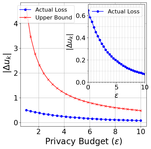

The experimental setup is as in Sec. VI-VI-A-VI-A1. Performance is benchmarked in terms of the utility loss in (12). Figure 5(a) shows the utility loss for , along with the upper bound from Theorem IV.4. The upper bound is tight only for large due to the union bound and Bernstein inequality. Figure 5(b) shows the utility loss versus for the existing approach.
From Figures 5(a) and 5(b), we observe:
- 1.
As (or ) increases (reduced privacy), the empirical utility loss decreases.
- 2.
- 3.
Hence, Algorithm 1 offers a better trade-off between privacy and utility loss.
Disadvantages of the existing approach in [10]:
(i) The optimization problem in (22) is a batch problem, unsuitable for online electronic warfare scenarios, whereas Algorithm 1 operates online with minimal controller modifications. (ii) There is no formal privacy guarantee for the approach in [10]: the feasibility margin is reduced against revealed-preference learners, but no guarantee exists against other inference strategies.VI-B Masking the Dynamic Utility of CR
We consider a cognitive radar operating in a dynamic decision-making environment, switching between operating modes—such as scanning and tracking—according to a stationary policy , as described in Sec. V-V-A. The radar employs Algorithm 2, which perturbs the vMF-distributed utility prior to policy computation, obfuscating the radar’s latent utility from the adversary. To evaluate this concealment against an adversary performing inverse learning, we consider PolicyWalk [54] (Algorithm C) applied to demonstrations generated both with and without the utility perturbation, and examine whether the radar’s true preference ordering between operating states can still be recovered from the resulting posterior.
VI-B1 Qualitative Analysis

We use the same four-state, two-action MDP , , , with transition probability matrix adopted from the illustrative MDP in [54], where is a higher-SINR radar state than . For this case study, we consider the utility to depend only on the state, , rather than on the state–action pair as in Sec. V-V-A. As in the static setting, is drawn from the stochastic linear utility model of Sec. IV-IV-C, with and , which concentrates mass on utility vectors satisfying — the radar’s physically motivated preference for the higher-SINR state , whose stronger detection and tracking performance makes it the dominant operating choice whenever reachable. Recovering this ordering is the “cognition” an adversary performing inverse learning seeks to expose: with PolicyWalk, the recovered posterior reflects a similar preference as the true utility, whereas under Algorithm 2, this preference is no longer exactly identifiable.
We evaluate the proposed mechanism by comparing two cases. In Case 1 (without distribution privacy), the radar computes its policy directly from the true utility , generates demonstrations accordingly, and the adversary recovers a posterior over using PolicyWalk (Algorithm C), following the likelihood, prior, and sampling procedure of [54]. In Case 2 (with Algorithm 2), the true utility is instead perturbed as , with drawn i.i.d. Laplace at scale for privacy budget ; the radar re-solves its policy under , generates a fresh set of demonstrations, and the adversary re-runs PolicyWalk identically to recover a second posterior. Comparing the two recovered posteriors thus directly reveals how effectively Algorithm 2 conceals the radar’s true preference ordering. We repeat this over 200 Monte Carlo trials and report all four resulting point clouds together with their means.
Case 1: Without distribution privacy: Panels (a)–(b)
The sampled true utilities (a) lie almost entirely above the diagonal, confirming with high consistency, and the mean (red marker) sits well above it. The recovered posterior (b) stays concentrated above the diagonal with its mean close to that in (a), correctly recovering the radar’s preference ordering in nearly all trials.
Case 2: With Algorithm 2: Panels (c)–(d)
Once is perturbed, the resulting (c) is visibly more dispersed, with a non-negligible fraction of samples now falling on or below the diagonal — the ordering degrades at the level of the utility itself, before any inference takes place. The corresponding posterior (d) straddles the diagonal, with its mean shifting noticeably toward it relative to (b), showing that the preference ordering is recovered far less reliably. This degradation follows from Algorithm 2 propagating through the radar’s policy, its demonstrations, and the PolicyWalk posterior — confirming that privatising the utility alone is sufficient to conceal the radar’s SINR-driven preference from an adversary.
VI-B2 Quantitative Analysis
We consider an MDP with states and actions, giving , as in Sec. V-V-A. The SINR ranges from dB to dB. The radar selects among . The utility function and transition probability matrix are adopted from [9].
Existing methodology: We benchmark Algorithm 2 against two prior approaches. [8, 9] models the multi-function radar’s controller as an MDP with state–action cost , and formulates the unperturbed sensing plan as the cost-minimizing occupancy-measure LP
| (23) |
subject to the same constraints as in (17); the resulting optimal policy is deterministic.
To mask the sensing plan, [9] perturbs away from while penalizing the determinant of the adversary’s Fisher Information Matrix (FIM), , as follows:
| (24) |
where trades off cost perturbation against Fisher information reduction, subject to the same constraints again as in (17). Although admits a closed-form expression, it is nonlinear in , so the resulting optimisation is non-convex, and provides no formal statistical guarantee, such as -DistP, on what the adversary can infer about the radar’s sensing plan.
In addition, prior work [11] takes a structurally different approach: rather than perturbing the policy or the utility, it perturbs the transition probability matrix of the MDP directly, prior to policy synthesis, via a Dirichlet mechanism with concentration parameter , and synthesises the policy for the resulting privatised MDP. We investigate this approach in the cognitive radar setting using the same MDP formulation as in Sec. V-V-A. Smaller increases randomness and hence strengthens privacy, at the cost of a larger deviation of the resulting policy’s value from that under the true transition probabilities – termed the “cost of privacy” in [11]; larger weakens privacy but reduces this cost. We vary .
Quantitative Comparison: As shown in Fig. 7(a), adversarial Fisher information decreases as privacy increases across all three approaches. For the proposed method, the decrease is gradual; for the -based approach [9], it is approximately constant up to a threshold and then sharply declines. The proposed method achieves the largest overall reduction in adversarial Fisher information among the three approaches, outperforming both existing baselines. Moreover, the existing methods require either explicit Fisher information constraints (leading to non-convex optimisation, as in [9]) or perturbation of the transition probability matrix , as in [11]. Transition perturbation may not always be appropriate for cognitive radar systems, since the transition dynamics depend on external factors such as target motion and channel conditions, as well as the already-designed radar system.

(a)

(b)
The proposed method does incur a moderate utility deviation relative to the existing approaches, as shown in Fig. 7(b); this is the price paid for achieving a formal -DistP guarantee without relying on Fisher information constraints or transition-matrix perturbation, and is consistent with the analytical bound in Theorem V.2. Operating directly on the vMF-distributed utility with the same Laplace-noise mechanism as WDPCH-SU (Algorithm 1), scaled to dimension , this deviation remains bounded and predictable. Across all three approaches, utility deviation increases with privacy, confirming the inherent privacy–performance trade-off characterised in Theorem V.2.
VII Conclusion
In this article, we proposed an online ECCM framework to conceal the strategic decision-making of a cognitive radar (CR) against adversarial inference. The radar’s utility function was modeled via a von Mises–Fisher (vMF) distribution under two complementary paradigms: a static constrained utility-maximization setting and a dynamic expected utility-maximization. We adopted a distribution privacy framework, developing WDPCH-SU and WDPCH-DU for the static and dynamic settings, respectively, each injecting Laplace-calibrated noise into the vMF-distributed utility prior to policy computation, with formal -DistP guarantees established for each. Analytical bounds characterizing the privacy–performance trade-off were derived, quantifying utility loss (static) and expected utility deviation (dynamic) as functions of . Numerical results show that, in comparison with existing methodology, WDPCH-SU achieves lower utility loss and stronger privacy than [10], while WDPCH-DU attains a greater reduction reduction in adversarial Fisher information than existing approaches, without requiring explicit Fisher information constraints [9] or transition probability perturbation [11]—both with minimal modification to baseline radar controllers.
In this appendix, we document the algorithms used for adversarial inference and privacy-preserving policy synthesis.
Algorithm A implements the Metropolis–Hastings (MH) MCMC procedure used by the adversary to infer the posterior distribution of the radar’s cognitive parameter from the observed dataset , by iteratively sampling candidate parameters and accepting or rejecting them via a likelihood ratio test.
Step 5 of Algorithm A requires the computation of likelihood. The likelihood can be computed numerically as follows. Each observation represents a region , such that is the solution of (9) for all , i.e., Given the parameter , the likelihood of the dataset is
| (25) |
Algorithm B provides a sampling-based procedure to numerically evaluate the likelihood required in the MH acceptance ratio of Algorithm A, by drawing samples , solving the constrained LP in (9), and computing the fraction of samples whose optimal response matches the observed within a threshold .
Algorithm C is an MCMC sampling procedure adapted from the PolicyWalk algorithm of Ramachandran and Amir [54], used by the adversary to perform Bayesian inverse learning of the cognitive radar’s latent utility from the observed dataset . At each step, a neighbouring utility vector is proposed and accepted or rejected via a Metropolis–Hastings ratio , with the policy updated through warm-started policy iteration whenever violates the Bellman optimality condition; the resulting sample mean converges to , the adversary’s estimate of the radar’s true utility.
Algorithm D perturbs the transition probability matrix of the dynamic-utility CR model using Dirichlet noise [11]: the transition probabilities are privatised by applying a Dirichlet mechanism independently to each row, yielding , and the optimal radar policy is then synthesised for the privatised MDP via standard Bellman equations, where the concentration parameter controls the privacy–utility trade-off: smaller introduces higher perturbation and stronger privacy, while larger preserves the original transition structure more closely.
References
- [1] (2006) Cognitive radar: a way of the future. IEEE Signal Processing Magazine 23 (1), pp. 30–40. Cited by: §I, §II, §IV-A.
- [2] (2020) Cognitive radar. Technical report Technical Report AC/323 (SET-227) TP/947, NATO Science and Technology Organization (STO), Neuilly-Sur-Seine Cedex, France. Cited by: §I.
- [3] (2016) Coordinate descent for cognitive radar adaptation. In Proc. CIE International Conference on Radar (RADAR), pp. 1–5. Cited by: §I, §IV-A.
- [4] (2015) Cognitive radar framework for target detection and tracking. IEEE Journal of Selected Topics in Signal Processing. Cited by: §I, §II, §IV-A, item iii.
- [5] (2016) Multiple target tracking in the fully adaptive radar framework. In Proc. IEEE Statistical Signal Processing Workshop (SSP), pp. 1–5. Cited by: §I.
- [6] (2022) The development of radar and radar countermeasure. Springer, Singapore. Cited by: §I.
- [7] (2022) Principal–agent problem as a principled approach to eccm in radar. IEEE Trans. Aerosp. Electron. Syst. 58 (4). Cited by: §I, §II-B.
- [8] (2024) Masking the sensing plan for multifunction radar in an adversarial setting. In Proc. IEEE Radar Conf., Cited by: §I, §II-C, §V-A, §V-B, §VI-B2.
- [9] (2025) Fisher information approach for masking the sensing plan. IEEE Transactions on Aerospace and Electronic Systems 61 (1), pp. 233–249. Cited by: item 5, §I, §II-C, §V-A, §V-B, Fig. 7, Fig. 7, §VI-B2, §VI-B2, §VI-B2, §VI-B2, §VII.
- [10] (2023) Metacognitive radar: masking cognition from an inverse reinforcement learner. IEEE Trans. Aerosp. Electron. Syst. 59 (6). Cited by: item 5, §II-C, Fig. 5, Fig. 5, item 2, item ii, §VI-A2, §VI-A2, §VI-A2, §VI-A2, §VII.
- [11] (2020) Privacy-preserving policy synthesis in markov decision processes. In Proc. IEEE Conf. Decision and Control (CDC), Cited by: item 5, §II-D, Fig. 7, Fig. 7, §VI-B2, §VI-B2, §VII, §VII.
- [12] (2003) Adaptive radar: evolution to cognitive radar. In Proc. IEEE Int. Symp. Phased Array Systems and Technology, Cited by: §II.
- [13] (2012) Cognitive dynamic systems: perception–action cycle, radar and radio. Cambridge Univ. Press. Cited by: §II, §IV-A.
- [14] (2004) Radar signals. Wiley. Cited by: §II-A.
- [15] (2008) Radar handbook. McGraw-Hill. Cited by: §II-A.
- [16] (1997) Theory of partially adaptive radar. IEEE Trans. Aerosp. Electron. Syst. 33 (4), pp. 1309–1325. Cited by: §II-A.
- [17] (1998) Benchmark for radar allocation and tracking in ecm. IEEE Trans. Aerosp. Electron. Syst. 34 (4), pp. 1097–1114. Cited by: §II-A.
- [18] (2010) Principles of modern radar: basic principles. SciTech. Cited by: §II-A.
- [19] (2012) The mimo radar and jammer games. IEEE Trans. Signal Process. 60 (2), pp. 687–699. Cited by: §II-B.
- [20] (2015) Equilibrium between a statistical mimo radar and a jammer. In IEEE Radar Conf., Cited by: §II-B.
- [21] (2019) Deep q‑network based anti‑jamming strategy design for frequency agile radar. In International Radar Conference, pp. 1–5. Cited by: §II-B.
- [22] (2023) Radar jamming decision-making in cognitive electronic warfare: a review. IEEE Sensors Journal 23 (11), pp. 11383–11403. Cited by: §II-B.
- [23] (2000) Algorithms for inverse reinforcement learning. In ICML, Cited by: §II-B.
- [24] (2004) Apprenticeship learning via inverse reinforcement learning. In ICML, Cited by: §II-B.
- [25] (2020) Inverse filtering for counter-autonomous systems. IEEE Trans. Signal Inf. Process. Netw.. Cited by: §II-B, §IV-B.
- [26] (2019) How to calibrate your adversary’s capabilities? inverse filtering for counter-autonomous systems. IEEE Trans. Signal Process. 67 (24), pp. 6511–6525. Cited by: §II-B, §IV-A, §IV-B, item iii.
- [27] (2020) Identifying cognitive radars—inverse reinforcement learning using revealed preferences. IEEE Trans. Signal Process. 68, pp. 4529–4542. Cited by: §II-B, §IV-A, §IV-A, §IV-C, item iii.
- [28] (2025) Bayesian inverse learning and online changepoint detection of cognitive radar strategies. IEEE Transactions on Radar Systems 3, pp. 562–575. Cited by: §II-B, §IV-A, §IV-A, §IV-C, §IV-C.
- [29] (2020) Sensor selection for multi-target tracking in phased array radar network under hostile environment. Proc. IEEE Radar Conf., pp. 1–5. Cited by: §II-B.
- [30] (2023) Improving anti-jamming decision making strategies for cognitive radar via multi-agent deep reinforcement learning. Digit. Signal Process. 135, pp. 103952. Cited by: §II-B.
- [31] (2021) Constrained online learning to mitigate distortion effects in pulse-agile cognitive radar. Proc. IEEE Radar Conf., pp. 1–6. Cited by: §II-B.
- [32] (2022) Adversarial multi-player bandits for cognitive radar networks. In IEEE Radar Conf., Cited by: §II-B.
- [33] (2023) Smart interference signal design to a cognitive radar. Proc. IEEE Radar Conf., pp. 1–6. Cited by: §II-B.
- [34] (2020) Optimal stealthy deception attack against cyber-physical systems. IEEE Transactions on Cybernetics 50 (9), pp. 3963–3972. Cited by: §II-C.
- [35] (2022) Deception in supervisory control. IEEE Transactions on Automatic Control 67 (2), pp. 738–753. Cited by: §II-C.
- [36] (2020) Entropy maximization for markov decision processes under temporal logic constraints. IEEE Transactions on Automatic Control 65 (4), pp. 1552–1567. Cited by: §II-C.
- [37] (2019) Least inferable policies for markov decision processes. In Proceedings of the American Control Conference (ACC), pp. 1224–1231. Cited by: §II-C.
- [38] (1993) Fundamentals of statistical signal processing: estimation theory. Prentice-Hall, Englewood Cliffs, NJ, USA. Cited by: §II-C.
- [39] (2004) Accurate estimation of the fisher information matrix for the pet image reconstruction problem. IEEE Trans. Med. Imag. 23 (9), pp. 1057–1064. Cited by: §II-C.
- [40] (2019) On bayesian fisher information maximization for distributed vector estimation. IEEE Trans. Signal Inf. Process. Netw. 5 (4), pp. 628–645. Cited by: §II-C.
- [41] (2021) On the variance of the fisher information for deep learning. In NeurIPS, Vol. 34, pp. 5708–5719. Cited by: §II-C.
- [42] (2006) Differential privacy. In ICALP, Cited by: §II-D, §IV-D, §V-D.
- [43] (2014) The algorithmic foundations of differential privacy. Foundations and Trends in Theoretical Computer Science. Cited by: §II-D.
- [44] (2019) Local obfuscation mechanisms for hiding probability distributions. In ESORICS, Cited by: §II-D.
- [45] (2017) Pufferfish privacy mechanisms for correlated data. In SIGMOD, Cited by: §II-D.
- [46] (2023) Protecting global properties of datasets with distribution privacy mechanisms. In AISTATS, Cited by: §II-D, Definition III.1, §IV-D, §V-D.
- [47] (2019) How to calibrate your adversary’s capabilities? inverse filtering for counter-autonomous systems. IEEE Transactions on Signal Processing 67 (24), pp. 6511–6525. Cited by: §IV-A.
- [48] (2022) Inverse cognition in nonlinear sensing systems. In Proc. Asilomar Conf. Signals, Systems, and Computers, pp. 1116–1120. Cited by: §IV-A.
- [49] (2009) Directional statistics. 2nd edition, Wiley, Chichester, UK. Cited by: §IV-C, §V-C.
- [50] (1994) Markov decision processes: discrete stochastic dynamic programming. Wiley. Cited by: §V-A.
- [51] (1999) Constrained markov decision processes. CRC Press. Cited by: §V-A.
- [52] (2012) Revealed preference and its applications. Economic Journal 122 (560), pp. 332–338. Cited by: §VI-A2.
- [53] (1967) The construction of utility functions from expenditure data. International Economic Review 8 (1), pp. 67–77. External Links: Document Cited by: §VI-A2.
- [54] (2007) Bayesian inverse reinforcement learning. In IJCAI, Cited by: §VI-B1, §VI-B1, §VI-B, §VII, 3.