Detect Anything in Graphic Design:
Element-Level Rewards for Autoregressive Detection

Jiangning Zhu Affiliation: BNRist, Tsinghua University Bowen Li Affiliation: BNRist, Tsinghua University Shenyu Qiao Affiliation: BNRist, Tsinghua University Yima Gu Affiliation: BNRist, Tsinghua University Zhao Zhang, Yuhui Yuan , Shixia Liu ^†^†thanks: Corresponding author. Affiliation: BNRist, Tsinghua University Affiliation: Canva Research

Abstract

Graphic designs, such as posters, advertisements, and infographics, are an important medium for communicating information and shaping understanding. Unlike natural images, they consist of layered elements with explicit compositional order. However, existing object detection models treat these elements as an unordered set, leaving compositional order unexploited. To address this limitation, we present Detect Anything in Graphic Design (DAD), a model that formulates graphic design detection as compositional deconstruction. It decodes elements in compositional order, using lower-layer elements to better detect higher-layer ones. The key feature of DAD is amodal detection, which predicts the full bounding box of each element, including regions occluded by elements placed above it. Building on this formulation, we propose Element Relative Policy Optimization (EleRPO), which extends GRPO from sequence-level supervision to element-level optimization. EleRPO provides fine-grained training signals that capture how each detected element contributes to overall detection quality, and works synergistically with compositional order to improve detection performance. To support training and evaluation, we build a dataset of 10 million graphic designs. Experiments show that DAD outperforms all baselines and achieves human-level performance in amodal detection, supporting effective image-to-layer decomposition. EleRPO consistently improves over GRPO across nine detection benchmarks.

Code: https://github.com/dad887/DAD

Data & Dataset Card: https://huggingface.co/datasets/dad887/DAD

Refer to caption — Figure 1: The DAD model detects elements missed by GPT-5.5 and recovers occluded regions. It performs the best across all datasets and metrics. Metrics are normalized to $[0.1,1]$ in radar charts.

1 Introduction

Graphic designs, such as posters, advertisements, and infographics, are a ubiquitous visual medium that shapes how people consume information across business communication, news media, public services, and education. By combining text with visual elements such as photographs, pictograms, and diagrams, they clearly organize complex information, attract attention, and make ideas easier to understand. A key property that distinguishes graphic designs from natural images is their compositional nature. They are typically built from discrete, layered elements that are arranged in a deliberate visual order and often partially or fully occlude one another. This layered structure is central to how designs are created, interpreted, edited, and reused. Consequently, access to layer-level representations is essential for understanding and modifying graphic designs [77, 31]. In practice, however, graphic designs are often distributed as flat raster images (e.g. , JPEG or PNG) for compatibility, which removes explicit layer information and makes subsequent editing difficult. Recovering the underlying layers from a flat image is therefore a key step for downstream applications [70]. A fundamental task in this process is graphic design detection, which aims to identify the locations, categories, and compositional order of design elements [58].

Recent advances in visual recognition and object detection [80, 66, 33] have led to increasingly capable models that accurately localize and categorize a broad range of objects. However, these models are primarily designed for natural images [21, 52] or text-dominant documents [17, 57, 48], which introduces two key limitations when applied to graphic design detection. First, objects in these two domains generally lack an intrinsic compositional order, so existing models represent them as an unordered set and can not predict the compositional order of the elements. Without this order, the recovered elements can not be faithfully recomposed into the original design. Second, because annotating large-scale occluded regions is challenging, existing models are usually trained to predict only visible regions. As a result, the hidden parts of partially occluded elements remain unrecovered. These limitations call for a graphic design detection model that can infer compositional order while also learning to recover occluded regions from large-scale annotated data.

To fill this gap, we present Detect Anything in Graphic Design (DAD), a model for graphic design detection. Building upon autoregressive detection with vision-language models (VLMs) [21, 5], DAD formulates graphic design detection as compositional deconstruction and predicts elements in compositional order. Each element is specified by its category and an amodal bounding box that captures its full spatial extent, including the regions occluded by the elements above it. With compositional order, DAD uses lower-layer elements as context when detecting a higher-layer one, aligning with the layer-by-layer process by which designers construct graphic designs. Based on this formulation, we propose Element Relative Policy Optimization (EleRPO), which extends Group Relative Policy Optimization (GRPO) [55] from sequence-level supervision to element-level optimization. At the core of EleRPO is the martingale difference decomposition [64], which decomposes a sequence-level reward into unbiased, history-conditioned element-level rewards. Estimating this reward requires no additional reward models or extra sampling passes, making it a simple drop-in replacement for GRPO and applicable to any VLM-based detection model. To support the training and evaluation of DAD, we construct a large-scale dataset of $10$ million graphic designs, DAD-10M. The dataset is anchored by a corpus of $5$ million designer-created works, from which we extract ground-truth amodal bounding boxes and compositional order using their original layered representations. To further improve the diversity of occluded elements and styles, we augment this corpus with an additional $5$ million designs, including those constructed via element replacement, as well as designer-created and AI-generated flat designs.

We validate the effectiveness of DAD and EleRPO through comprehensive experiments. DAD achieves better detection performance than both proprietary and open-source baselines on our dataset, and these gains transfer to existing graphic design detection benchmarks (Fig. 1). Human evaluation further shows that DAD achieves human-level accuracy in predicting the occluded regions of elements. In addition, EleRPO consistently improves over GRPO and other fine-grained reinforcement learning (RL) methods, such as PRIME [7] and VinePPO [22], and generalizes across detection models and a wide range of detection benchmarks.

The main contributions of this work are threefold:

•

We develop a graphic design detection model, DAD, that predicts the amodal bounding boxes of elements in their compositional order.
•

We propose an optimization method, EleRPO, that extends GRPO to element-level supervision by decomposing sequence-level rewards into a martingale difference sequence.
•

We release a subset of DAD-10M containing $100,000$ designs for image-to-layer decomposition, each with original layer representations and diverse element styles.

2 Related Work

Autoregressive Object Detection

Object detection has evolved from set-based detectors [3, 73, 79, 35, 20] to autoregressive detectors with fixed categories [5, 6, 61, 37], and more recently to promptable VLM-based models for open-vocabulary detection [63, 65, 21, 56] and grounding [47, 71]. These advances have also influenced structured document domains, where layout-aware document understanding models [68, 67, 17, 29, 32], specialized layout detectors [74, 57], and benchmarks [75, 48, 26, 44, 13] have supported structured document analysis. However, existing detectors represent objects as an unordered set, and thus cannot recover the compositional order and occluded regions required for layer reconstruction. Closing this gap typically requires learning this information from human annotations [78, 50], which are difficult to scale and can be imprecise. In contrast, DAD learns from exact ground truth extracted at scale from original layered representations, enabling compositional-order prediction and occluded-region recovery.

Reward Design for RL Post-Training

A common RL algorithm is GRPO [55], which assigns a sequence-level reward uniformly to all tokens. Existing extensions to finer-grained supervision can be grouped into two categories: policy-signal-based methods and re-rollout-based methods. Policy-signal-based methods derive fine-grained supervision from the current rollout, either by directly using policy statistics [59, 45], or by learning reward models over intermediate states [7, 28, 53]. Re-rollout-based methods produce fine-grained supervision by sampling additional rollouts and comparing them [22, 11, 1, 24]. These methods are designed for settings where intermediate tokens can not be directly evaluated. Therefore, they rely on proxy supervision that is not directly aligned with the final reward. In detection tasks, however, each predicted element contributes measurably to the final reward. EleRPO exploits this property to derive element-level rewards via martingale difference decomposition, without requiring additional reward models or re-rollouts. To our knowledge, EleRPO is the first method that leverages the inherent decomposability of detection rewards.

3 Method

We formulate graphic design detection as compositional deconstruction, introduce EleRPO for element-level optimization, and construct DAD-10M, a 10-million dataset with layer annotations.

3.1 Task Formulation

Predicting the compositional order from an image is challenging because occlusion relationships are implicit, and the model must infer which element lies above the other when they overlap. We address this by formulating graphic design detection as compositional deconstruction, where elements are generated sequentially in compositional order. Given an input image $I$ , the model predicts an element sequence $(e_{1},\dots,e_{m})$ with policy $e_{k}\sim\pi_{\theta}(\cdot|e_{<k},I)$ , using previously predicted lower-layer elements $e_{<k}$ as context for the higher-layer one $e_{k}$ . Sec. 4.2.2 shows that this formulation performs better than alternative element orderings.

3.2 Element Relative Policy Optimization

GRPO optimizes a sequence-level reward that measures the overall quality of predicted elements [21, 56]. In our implementation, we use the IoU-weighted $F_{1}$ [21], a commonly used reward function that reflects localization accuracy, precision, and recall. It is computed by matching predicted elements to ground truth via spatial overlap, assigning each prediction a score $s_{i}$ equal to its IoU if the category is correct, and 0 otherwise, and then calculating the $F_{1}$ score from these scores. GRPO assigns the same sequence-level advantage to all tokens, thereby ignoring each element’s contribution to the final detection quality. As a result, an inaccurately predicted element in a high-reward rollout still receives a positive advantage, inadvertently reinforcing incorrect predictions. To address this limitation, we first decompose the sequence-level reward into element-level rewards via martingale difference decomposition. We then estimate the element-level rewards from a group of sampled rollouts and convert them into the advantages for policy updates.

3.2.1 Element-Level Reward via Martingale Difference Decomposition

Ideal element-level rewards $\{r_{k}\}_{k=1}^{m}$ should satisfy three properties:

1.

Completeness: $\sum_{k=1}^{m}r_{k}=F_{1}-\mathbb{E}[F_{1}|I]$ . The rewards should sum to the total change of the final $F_{1}$ score over its expectation before any element is generated.
2.

Causality: $r_{k}$ depends only on $e_{\leq k}$ . Since elements are generated autoregressively, the reward for $e_{k}$ should depend only on the lower-layer elements, without access to higher-layer elements.
3.

Unbiasedness: $\mathbb{E}[r_{k}|e_{<k},I]=0$ . The reward should isolate the contribution of $e_{k}$ itself and not be biased by lower-layer elements.

These properties uniquely define the element-level rewards as the martingale differences [64] of $F_{1}$ , which captures how the conditional expected $F_{1}$ evolves as elements are generated:

r_{k}=\mathbb{E}[F_{1}|e_{\leq k},I]-\mathbb{E}[F_{1}|e_{<k},I].

(1)

The conditional expectation $\mathbb{E}[F_{1}|e_{\leq k},I]$ decomposes into $F_{1}(k)$ and the expected remaining improvement $\mathbb{E}[F_{1}-F_{1}(k)|e_{\leq k},I]$ . Here, $F_{1}(k)$ is the score computed by comparing the lower-layer elements $e_{\leq k}$ with the ground-truth elements. Substituting this decomposition into Eq. (1) gives:

r_{k}=\Delta F_{1}(k)-(\mathbb{E}[F_{1}{-}F_{1}(k{-}1)|e_{<k},I]-\mathbb{E}[F_{1}{-}F_{1}(k)|e_{\leq k},I]),

(2)

where $\Delta F_{1}(k){=}F_{1}(k){-}F_{1}(k{-}1)$ is the change in $F_{1}$ score after adding $e_{k}$ to the lower-layer elements $e_{<k}$ . Detailed proofs are provided in Appendix A.1.

3.2.2 Advantage Estimation from Sampled Rollouts

While Eq. (2) defines the ideal element-level reward, exactly computing the expected improvements, $\mathbb{E}[F_{1}{-}F_{1}(k{-}1)|e_{<k},I]$ and $\mathbb{E}[F_{1}{-}F_{1}(k)|e_{\leq k},I]$ , is intractable. As shown in Fig. 2, we approximate them using rollouts sampled for each image, and then estimate the element-level rewards.

A key challenge is that different rollouts have different lower-layer elements $e_{<k}$ , making their expected improvement not directly comparable. Under the compositional order, however, rollouts naturally form clusters based on the detection quality of lower-layer elements, and rollouts within the same cluster exhibit similar expected improvement in $F_{1}$ . Inspired by Pavlenko et al. [46], we group rollouts with similar $F_{1}(k{-}1)$ and approximate $\mathbb{E}[F_{1}{-}F_{1}(k{-}1)|e_{<k},I]\approx\mathbb{E}[F_{1}{-}F_{1}(k{-}1)|F_{1}(k{-}1),I]$ . In practice, we partition the rollouts into $N_{c}$ clusters using k-means on $F_{1}(k{-}1)$ , where $N_{c}$ is selected based on the silhouette score. This approximation avoids additional re-rollouts, yet achieves a Pearson correlation of $0.81$ with an expensive but accurate re-rollout-based estimator. We use the same clusters to estimate both expected improvements in Eq. (2). This makes their difference a paired comparison across the same rollouts, avoiding the bias introduced by using different clusters. Let $\mathcal{C}_{k}(i)$ denote the cluster containing rollout $i$ . The element-level reward is then estimated as:

\hat{r}_{k}^{(i)}=\Delta F_{1}^{(i)}(k)-\frac{1}{|\mathcal{C}_{k}(i)|}\sum\nolimits_{j\in\mathcal{C}_{k}(i)}\Delta F_{1}^{(j)}(k).

(3)

Detailed derivations, the justification for using the same clusters, and the details on the empirical validation are provided in Appendix A. The magnitude of $\hat{r}_{k}^{(i)}$ scales as $\mathcal{O}(1/(k+n))$ , where $n$ is the number of ground-truth elements (see Appendix A.4 for the proof). Without correction, the lower-layer elements would dominate policy updates because their rewards have larger magnitudes. To address this, we normalize the reward by the layer-wise standard deviation. Let $\mathcal{G}_{k}$ denote the set of rollouts that contain at least $k$ elements. The element-level advantage is:

\hat{A}_{k}^{(i)}=\hat{r}_{k}^{(i)}\big/\sqrt{\frac{1}{|\mathcal{G}_{k}|}\sum\nolimits_{j\in\mathcal{G}_{k}}(\hat{r}_{k}^{(j)})^{2}+\epsilon}.

(4)

While $\hat{A}_{k}^{(i)}$ provides fine-grained supervision, it is estimated from a finite group of rollouts and can be noisy. To improve stability, we combine it with the sequence-level GRPO advantage $\hat{A}^{(i)}$ :

$\mathcal{J}_{\text{{EleRPO}}}(\theta)=\frac{1}{G}\sum_{i=1}^{G}\frac{1}{|o^{(i)}|}\sum_{t=1}^{|o^{(i)}|}\left[\min\!\Big(\rho_{i,t}\tilde{A}_{\phi(i,t)}^{(i)},\;\text{clip}(\rho_{i,t},1-\epsilon,1+\epsilon)\tilde{A}_{\phi(i,t)}^{(i)}\Big)-\beta\mathbb{D}_{\text{KL}}[\pi_{\theta}\|\pi_{\text{ref}}]\right]$

(5)

where $\tilde{A}_{\phi(i,t)}^{(i)}=\tfrac{1}{2}\big(\hat{A}_{\phi(i,t)}^{(i)}+\hat{A}^{(i)}\big)$ , and $\phi(i,t)$ maps token $o_{t}^{(i)}$ to its corresponding element.

3.3 Dataset Construction

We construct the dataset, DAD-10M, in two stages: data collection and data selection.

Data collection

The dataset is anchored by an internal corpus of $5,367,586$ designer-created works. These works preserve their original layered representations, so we automatically extract ground-truth amodal bounding boxes and compositional orders. Such annotations would be infeasible to obtain manually at this scale. To further improve diversity, we augment this corpus with three sources: 1) $2,075,896$ designs created by replacing elements with stylistically and semantically similar ones retrieved from a pool of 12 million elements; 2) $127,931$ designs generated using Ideogram [19] and annotated by Gemini-3-Pro [9]; and 3) $2,845,242$ internal flat designer-created designs annotated by Gemini-3-Pro. Together, these sources result in a dataset of $10,416,655$ designs. For public data release, we sample $100,000$ designs with replaced elements, each annotated with the original layer representations.

Data selection

Despite the availability of layer annotations, the model still faces granularity ambiguity: semantically independent elements may be merged into one (e.g. , a cluster of decorative stars), while a single coherent element may be split into multiple parts (e.g. , a logo decomposed into several decorative shapes). We address this issue with a two-step filtering process. First, to improve the separation of small, independent elements, we train a preliminary detector and retain designs that achieve low recall for such elements. These designs provide useful supervision for learning to separate elements that are easily merged. Second, to discourage over-splitting, we filter out designs containing many small, mutually overlapping elements clustered in a small region, as these often correspond to parts of a single coherent element. This process yields $24,195$ high-quality designs, which we split into $19,195$ designs for RL training and $5,000$ for testing.

More details on data collection and selection are provided in Appendix B.

3.4 Implementation Details

We build DAD upon Qwen3-VL-2B [2]. Each element is represented by a bounding box with coordinates normalized to $[0,1000]$ , and a category label indicating whether the element is text or visual. We train DAD with LoRA [16] using rank $32$ across all linear layers. We first perform supervised fine-tuning (SFT) for $650,000$ steps with a learning rate of $1e{-}4$ and a batch size of 64. This stage uses all data in DAD-10M except the RL training and test splits. This is followed by RL using EleRPO for $5,000$ steps, with $16$ rollouts per image and a learning rate of $5e{-}7$ . Following Liu et al. [34], we compute separate IoU-weighted $F_{1}$ rewards for text and visual elements, and use their average as the final reward. More training details are provided in Appendix C.

4 Experiments

4.1 Performance of DAD

To demonstrate the effectiveness of DAD, we compare it with state-of-the-art models, evaluate its amodal detection quality through human evaluation, and apply it to layer decomposition.

Table 1: Comparison of DAD with state-of-the-art baselines on graphic design benchmarks.

	DAD-10M test set				DMLB
Method	$F_{1}$ @[.5:.95] $\uparrow$	IoU-weighted $F_{1}$ $\uparrow$	Occluded R@[.5:.95] $\uparrow$	POA $\uparrow$	$F_{1}$ @[.5:.95] $\uparrow$	IoU-weighted $F_{1}$ $\uparrow$	Occluded R@[.5:.95] $\uparrow$	POA $\uparrow$
Rex-Omni	31.24	38.12	15.41	-	17.79	19.19	13.25	-
Gemini-3.1-Pro	32.58	39.95	25.15	16.56	44.17	52.60	42.68	22.57
GPT-5.5	40.89	49.46	34.26	25.42	61.05	70.24	61.35	34.17
DAD (Ours)	72.57	79.65	65.35	50.18	79.52	84.42	71.65	46.97
	Crello				PrismLayersPro
Method	$F_{1}$ @[.5:.95] $\uparrow$	IoU-weighted $F_{1}$ $\uparrow$	Occluded R@[.5:.95] $\uparrow$	POA $\uparrow$	$F_{1}$ @[.5:.95] $\uparrow$	IoU-weighted $F_{1}$ $\uparrow$	Occluded R@[.5:.95] $\uparrow$	POA $\uparrow$
Rex-Omni	26.04	33.97	22.31	-	35.14	38.29	25.42	-
Gemini-3.1-Pro	34.32	42.20	36.91	18.77	40.75	48.54	37.71	22.32
GPT-5.5	45.86	56.53	52.26	29.31	61.41	73.66	60.53	37.29
DAD (Ours)	57.75	68.31	58.03	34.89	73.21	78.44	72.67	43.87
	LICA				ChartGalaxy
Method	$F_{1}$ @[.5:.95] $\uparrow$	IoU-weighted $F_{1}$ $\uparrow$	Occluded R@[.5:.95] $\uparrow$	POA $\uparrow$	$F_{1}$ @[.5:.95] $\uparrow$	IoU-weighted $F_{1}$ $\uparrow$	Occluded R@[.5:.95] $\uparrow$	POA $\uparrow$
Rex-Omni	28.51	35.70	16.37	-	6.31	8.24	3.16	-
Gemini-3.1-Pro	39.42	47.90	35.53	22.17	12.29	17.95	9.27	6.92
GPT-5.5	45.92	54.95	45.10	29.53	6.85	9.42	2.98	1.12
DAD (Ours)	71.02	78.89	62.67	46.96	32.97	57.71	35.76	27.71

4.1.1 Comparison with State-of-the-Art

Datasets

We evaluate DAD on DAD-10M test set and five graphic design benchmarks: Design-Multi-Layer-Bench (DMLB) [49], Crello [69], PrismLayersPro [4], LICA [14], and ChartGalaxy [27]. The DAD-10M test set is held out from training, and a benchmark-wise overlap check finds no duplicates between DAD-10M and the five external benchmarks.

Evaluation metrics

We evaluate the performance from four aspects: 1) overall detection quality, measured by the $F_{1}$ score averaged over IoU thresholds from $0.5$ to $0.95$ ( $F_{1}$ @[.5:.95]) and the IoU-weighted $F_{1}$ ; 2) amodal detection quality, measured by recall on elements with at least 5% occluded area, averaged over IoU thresholds (Occluded R@[.5:.95]); 3) ordering accuracy, measured by the pairwise ordering accuracy (POA) [78], defined as the proportion of correctly ordered overlapping element pairs, where a pair is correct if both elements are matched to ground-truth elements and their predicted order matches the ground-truth order; and 4) inference efficiency, measured by the average inference time per design.

Baselines

We compare DAD with a set of representative proprietary and open-source models. For proprietary models, we use GPT-4o [40], GPT-5 [41], GPT-5.4 [42], GPT-5.5 [43], and Gemini-3.1-Pro [10]. For open-source models, we evaluate GLIP-L [25], Detic-B [76], Grounding DINO-B [35], Florence2-L [65], Qwen3-VL [2], InternVL3.5 [62], and Rex-Omni [21].

Dataset statistics, data overlap checks, and baseline implementations are detailed in Appendix D.

Results

We evaluate the models over $3$ runs and report their mean results, except for proprietary models, which are evaluated once due to the cost of API calls. Table 1 compares DAD with state-of-the-art proprietary baselines (Gemini-3.1-Pro and GPT-5.5) and open-source baseline (Rex-Omni). The full results, including the variance across runs and inference efficiency, are provided in Appendix E. DAD achieves the best performance across all six datasets, improving overall detection quality, amodal detection quality, and ordering accuracy. It is also more efficient than proprietary baselines and comparable to open-source ones. As shown in Fig. 1(a), DAD performs robustly across diverse designs, detecting elements missed by GPT-5.5 and recovering their occluded regions. More examples are provided in Appendix E.

4.1.2 Human Evaluation on Amodal Detection

Figure 3: Results of human evaluation on amodal detection.

Experimental setup

To evaluate DAD’s amodal detection quality, we compare its predictions with human annotations on $500$ occluded elements sampled from the DAD-10M test set. These elements are evenly distributed across five bins, ranging from $0$ %- $20$ % to $80$ %- $100$ % occluded area. We recruit $16$ annotators with at least one year of graphic design experience, and divide them into $4$ groups. Each group contains $4$ annotators and annotates the same $125$ elements. Annotators are shown only the visible region of each element and asked to label its amodal bounding box using a web-based annotation tool. The annotation interface and compensation details are provided in Appendix D.3. For each element, we obtain its predictions from DAD, GPT-5.5, and Gemini-3.1-Pro by selecting the one with the highest IoU. We then compute the average IoU between model predictions and human annotations. As a reference for human-level performance, we also compute inter-annotator IoU within each group.

Results

Fig. 3 compares the average IoU between each model and human annotators against the distribution of inter-annotator IoUs. GPT-5.5 and Gemini-3.1-Pro consistently fall below the inter-annotator IoU range across all occlusion levels. In contrast, DAD stays within this range, indicating that it achieves human-level amodal detection quality.

Table 2: Evaluation results on image-to-layer decomposition across graphic design benchmarks.

	DAD-10M test set						DMLB
Method	PSNR $\uparrow$	SSIM $\uparrow$	RGB L1 $\downarrow$	Alpha SIoU $\uparrow$	Occ-PSNR $\uparrow$	Occ-SSIM $\uparrow$	PSNR $\uparrow$	SSIM $\uparrow$	RGB L1 $\downarrow$	Alpha SIoU $\uparrow$	Occ-PSNR $\uparrow$	Occ-SSIM $\uparrow$
GT Box	30.23	0.955	0.188	0.592	15.42	0.468	29.28	0.947	0.213	0.553	19.79	0.572
Gemini-3.1-Pro	26.59	0.933	0.252	0.369	5.76	0.144	26.72	0.935	0.244	0.459	7.33	0.213
GPT-5.5	28.62	0.948	0.242	0.436	7.48	0.204	29.92	0.956	0.228	0.530	10.80	0.312
DAD (Ours)	29.83	0.953	0.223	0.511	12.20	0.357	30.10	0.957	0.210	0.571	14.23	0.383
	PrismLayersPro						Crello
Method	PSNR $\uparrow$	SSIM $\uparrow$	RGB L1 $\downarrow$	Alpha SIoU $\uparrow$	Occ-PSNR $\uparrow$	Occ-SSIM $\uparrow$	PSNR $\uparrow$	SSIM $\uparrow$	RGB L1 $\downarrow$	Alpha SIoU $\uparrow$	Occ-PSNR $\uparrow$	Occ-SSIM $\uparrow$
GT Box	31.02	0.950	0.178	0.499	12.04	0.417	27.44	0.913	0.125	0.783	13.87	0.415
Gemini-3.1-Pro	28.69	0.943	0.201	0.371	6.49	0.215	25.14	0.907	0.191	0.581	4.29	0.137
GPT-5.5	30.84	0.957	0.190	0.477	8.80	0.293	23.95	0.875	0.173	0.604	4.94	0.147
DAD (Ours)	31.40	0.959	0.186	0.482	9.72	0.325	27.83	0.930	0.162	0.642	5.74	0.180
	LICA						ChartGalaxy
Method	PSNR $\uparrow$	SSIM $\uparrow$	RGB L1 $\downarrow$	Alpha SIoU $\uparrow$	Occ-PSNR $\uparrow$	Occ-SSIM $\uparrow$	PSNR $\uparrow$	SSIM $\uparrow$	RGB L1 $\downarrow$	Alpha SIoU $\uparrow$	Occ-PSNR $\uparrow$	Occ-SSIM $\uparrow$
GT Box	29.98	0.952	0.195	0.637	14.97	0.443	30.80	0.974	0.235	0.426	18.25	0.506
Gemini-3.1-Pro	26.46	0.935	0.243	0.452	5.87	0.185	29.59	0.966	0.278	0.225	4.05	0.100
GPT-5.5	29.20	0.955	0.224	0.534	8.06	0.255	29.27	0.968	0.272	0.270	4.11	0.093
DAD (Ours)	29.81	0.956	0.222	0.550	9.94	0.324	30.10	0.972	0.270	0.328	9.79	0.270

4.1.3 Application to Image-to-Layer Decomposition

Experimental setup

We evaluate DAD on image-to-layer decomposition using the MRT model [60], which recovers the underlying layers of a flat image based on input bounding boxes of elements. We compare DAD with GPT-5.5 and Gemini-3.1-Pro by using their predicted bounding boxes as input to MRT, and evaluate the resulting layers on the same six datasets as in Section 4.1.1. As a reference, we also evaluate MRT with ground-truth boxes as input. We evaluate the performance from three aspects: 1) image-level recovery quality, measured by the PSNR and SSIM of the image recomposed from the predicted layers; 2) layer-level recovery quality, following LayerD [58], measured by RGB L1 (alpha-weighted L1 distance on RGB channels) and Alpha soft IoU (soft IoU on alpha channels) between predicted and ground-truth layers, allowing no adjacent-layer merges to jointly evaluate layer content and granularity; and 3) occlusion recovery quality, measured by the PSNR and SSIM computed on occluded pixels in the ground-truth layers, where predicted layers are matched to ground-truth layers using the Hungarian algorithm, and scores are averaged over occluded ground-truth layers, with unmatched layers assigned a score of $0$ .

Results

As shown in Table 2, DAD consistently outperforms GPT-5.5 and Gemini-3.1-Pro across all datasets, improving image-level, layer-level, and occlusion recovery quality. On image-level PSNR and SSIM, DAD matches the results achieved with ground-truth boxes, indicating that its predicted boxes are nearly as informative for recovering visible regions. As shown in Fig. 1(b), these predictions enable faithful layer recovery, including occluded regions missed by GPT-5.5.

4.2 Effectiveness of EleRPO

To demonstrate the effectiveness of EleRPO, we compare it with existing RL methods, conduct ablation studies on its key components, and evaluate its generalizability across models and benchmarks.

Table 3: Comparison of EleRPO with existing RL methods on DAD-10M.

SFT	GRPO	GRPO- $\lambda$	GTPO	PRIME	VinePPO	SPO	EleRPO (Ours)
54.8	74.2	73.0	74.1	73.3	58.0	57.9	79.7

4.2.1 Comparison with Existing Methods

Experimental setup

We compare EleRPO with GRPO and its finer-grained variants, including representative policy-signal-based methods (GRPO- $\lambda$ [45], GTPO [59], and PRIME [7]), as well as re-rollout-based methods (VinePPO [22] and SPO [11]). All the methods are applied to DAD-SFT, which denotes DAD after supervised fine-tuning, using the RL configuration in Sec. 3.4. Method-specific hyperparameters, such as the number of Monte Carlo continuations for VinePPO and SPO, follow the original papers. Additional details are provided in Appendix F.1. We evaluate all methods on DAD-10M test set using the training reward, IoU-weighted $F_{1}$ .

Results

As shown in Table 3, the policy-signal-based methods do not improve over GRPO, as they are designed for chain-of-thought reasoning and fail to capture each element’s contribution in detection. For example, GTPO assigns higher weights to high-entropy tokens, which are often low-order coordinate digits with limited impact on the final detection result. The re-rollout-based methods perform worse than GRPO because they are designed for tasks with discrete or binary outcomes, where a small number of rollouts can estimate success rates. In detection, however, reward changes are continuous and fine-grained, making them difficult to estimate reliably from the same number of rollouts. EleRPO addresses this limitation by directly decomposing the sequence-level reward into element-level rewards, outperforming GRPO and all other baselines.

Table 4: Ablation studies on key components of EleRPO.

(a) Reward causality

IoU	$\Delta F_{1}$
55.8	79.7

(b) Advantage Combination

Sequence-level	Element-level	Combined
74.2	78.5	79.7

	Random	Left-edge	Compositional
SFT	51.0	50.4	53.0
+ EleRPO	54.0	55.4	61.2

4.2.2 Ablation Studies

We conduct ablation studies on EleRPO from two perspectives: 1) destructive comparisons that validate the causal reward design, mean subtraction, and standard deviation normalization by intentionally violating each of them; and 2) comparisons of alternative choices for prefix clustering, advantage combination, and element order. The training and evaluation settings are the same as in Sec. 4.2.1, except for the comparison on element order, which requires a separate SFT stage as detailed in Appendix F.2. We report the results on reward causality, advantage combination, and element order in Table 4. The remaining ablations are provided in Appendix G.

Reward causality

We compare our element-level reward with a non-causal IoU-based reward, which replaces $\Delta F_{1}(k)$ with the IoU between each predicted element and its Hungarian-matched ground truth, or 0 if unmatched. Table 4(a) shows that this non-causal reward leads to a significant performance drop. This result highlights the importance of aligning the element-level reward with the autoregressive nature of VLM-based detection.

Advantage combination

Table 4(b) shows that using only the element-level advantage outperforms the sequence-level GRPO advantage, demonstrating the effectiveness of element-level optimization. Combining both further improves performance, indicating that the sequence-level advantage provides stable supervision that complements the fine-grained element-level advantage.

Element order

We compare three prediction orders: random, left-edge order that sorts elements by their leftmost x-coordinate, and compositional order. Table 4(c) compares their performance under two training settings: SFT alone and SFT followed by EleRPO. Compositional order improves performance with SFT alone, and the gain becomes large after applying EleRPO. This indicates that compositional order and element-level rewards are synergistic: element-level rewards are most informative when the prediction order preserves the underlying compositional structure, allowing marginal contributions to reflect the design logic.

4.2.3 Generalizability of EleRPO

Experimental setup

We evaluate the generalizability of EleRPO across models and benchmarks. We consider three models: DAD-SFT, Rex-Omni-SFT [21], and Qwen3-VL-2B fine-tuned on ChartGalaxy [27]. As shown in Table 5, we compare EleRPO with GRPO on benchmarks aligned with each model’s domain. These benchmarks cover three categories: 1) graphic layout benchmarks with underlying layer structure (ChartGalaxy [27] and Crello [69]); 2) layout benchmarks without explicit layer structure (Rico [8], PosterLayout [15], and DocLayNet [48]); and 3) natural image benchmarks (COCO [30], LVIS [12], BDD100K [72], and Objects 365 [54]). We perform the same overlap check as in Sec. 4.1.1 and find no duplicates between DAD-10M and these benchmarks. For each model-benchmark pair, we perform RL training and evaluation using the same setting as in Sec. 4.2.1. More details on the benchmarks are provided in Appendix F.3.

Table 5: Comparison of EleRPO with GRPO across different models and benchmarks.

(a) DAD-SFT

Method	ChartGalaxy	Crello	Rico	PosterLayout	DocLayNet	COCO
GRPO	56.5	56.8	49.4	63.9	48.4	38.9
EleRPO (Ours)	63.7	58.7	50.4	66.1	52.5	39.4

(b) Rex-Omni-SFT

Method	COCO	LVIS	BDD100K	Objects 365
GRPO	58.9	53.4	49.1	50.4
EleRPO (Ours)	59.7	53.9	49.7	51.0

Method	ChartGalaxy
GRPO	63.9
EleRPO (Ours)	66.4

Results

Table 5 shows that EleRPO consistently outperforms GRPO across all model-benchmark pairs. The largest gains are observed on graphic layout benchmarks, where the compositional structure makes element-level rewards particularly effective. EleRPO also achieves consistent gains on natural image benchmarks where such structure is absent, demonstrating its generalizability.

5 Conclusion

In this paper, we introduce DAD, a graphic design detection model based on compositional deconstruction. Instead of treating design elements as an unordered set, DAD models graphic designs as layered compositions, enabling amodal detection that recovers complete element boundaries even under occlusion. Experiments demonstrate the effectiveness of DAD for graphic design detection and its utility in downstream applications such as image-to-layer decomposition. Despite these promising results, several directions remain for future work. For example, extending this formulation to recover richer compositional structures beyond individual elements could benefit downstream tasks such as design editing, retrieval, and structured design analysis.

References

[1] A. Ahmadian, C. Cremer, M. Gallé, M. Fadaee, J. Kreutzer, O. Pietquin, A. Üstün, and S. Hooker (2024) Back to basics: revisiting REINFORCE-style optimization for learning from human feedback in LLMs. In Proceedings of the Annual Meeting of the Association for Computational Linguistics, pp. 12248–12267. Cited by: §2.
[2] S. Bai, Y. Cai, R. Chen, K. Chen, X. Chen, Z. Cheng, L. Deng, W. Ding, C. Gao, C. Ge, et al. (2025) Qwen3-vl technical report. arXiv preprint arXiv:2511.21631. Cited by: Appendix C, §D.2, §3.4, §4.1.1.
[3] N. Carion, F. Massa, G. Synnaeve, N. Usunier, A. Kirillov, and S. Zagoruyko (2020) End-to-end object detection with transformers. In Proceedings of European Conference on Computer Vision, pp. 213–229. Cited by: §2.
[4] J. Chen, H. Jiang, Y. Wang, K. Wu, J. Li, C. Zhang, K. Yanai, D. Chen, and Y. Yuan (2025) PrismLayers: open data for high-quality multi-layer transparent image generative models. arXiv preprint arXiv:2505.22523. Cited by: §D.1, §4.1.1.
[5] T. Chen, S. Saxena, L. Li, D. J. Fleet, and G. Hinton (2022) Pix2seq: a language modeling framework for object detection. In Proceedings of International Conference on Learning Representations, Cited by: §1, §2.
[6] T. Chen, S. Saxena, L. Li, T. Lin, D. J. Fleet, and G. Hinton (2022) A unified sequence interface for vision tasks. In Proceedings of Advances in Neural Information Processing Systems, Cited by: §2.
[7] G. Cui, L. Yuan, Z. Wang, H. Wang, Y. Zhang, J. Chen, W. Li, B. He, Y. Fan, T. Yu, et al. (2025) Process reinforcement through implicit rewards. arXiv preprint arXiv:2502.01456. Cited by: §F.1, §1, §2, §4.2.1.
[8] B. Deka, Z. Huang, C. Franzen, J. Hibschman, D. Afergan, Y. Li, J. Nichols, and R. Kumar (2017) Rico: a mobile app dataset for building data-driven design applications. In Proceedings of the annual ACM symposium on user interface software and technology, pp. 845–854. Cited by: §F.3, §4.2.3.
[9] Google DeepMind (2025) Gemini 3 Pro Model Card. Note: Accessed: 2026-02-04 External Links: Link Cited by: §3.3.
[10] Google DeepMind (2026) Gemini 3.1 Pro Model Card. Note: Accessed: 2026-05-01 External Links: Link Cited by: §D.2, §4.1.1.
[11] Y. Guo, L. Xu, J. Liu, D. Ye, and S. Qiu (2025) Segment policy optimization: effective segment-level credit assignment in RL for large language models. In Proceedings of The Annual Conference on Neural Information Processing Systems, Cited by: §F.1, §2, §4.2.1.
[12] A. Gupta, P. Dollar, and R. Girshick (2019) Lvis: a dataset for large vocabulary instance segmentation. In Proceedings of the IEEE/CVF conference on computer vision and pattern recognition, pp. 5356–5364. Cited by: §F.3, §4.2.3.
[13] I. Heo, T. Hwang, J. Jung, and S. Jung (2025) LED benchmark: diagnosing structural layout errors for document layout analysis. arXiv preprint arXiv:2507.23295. Cited by: §2.
[14] E. Hirsch, S. Yadav, M. Garg, and P. Mehta (2026) LICA: layered image composition annotations for graphic design research. arXiv preprint arXiv:2603.16098. Cited by: §D.1, §4.1.1.
[15] H. Y. Hsu, X. He, Y. Peng, H. Kong, and Q. Zhang (2023) Posterlayout: a new benchmark and approach for content-aware visual-textual presentation layout. In Proceedings of the IEEE/CVF Conference on Computer Vision and Pattern Recognition, pp. 6018–6026. Cited by: §F.3, §4.2.3.
[16] E. J. Hu, P. Wallis, Z. Allen-Zhu, Y. Li, S. Wang, L. Wang, W. Chen, et al. (2022) LoRA: low-rank adaptation of large language models. In International Conference on Learning Representations, Cited by: Appendix C, §3.4.
[17] Y. Huang, T. Lv, L. Cui, Y. Lu, and F. Wei (2022) Layoutlmv3: pre-training for document ai with unified text and image masking. In Proceedings of the ACM international conference on multimedia, pp. 4083–4091. Cited by: §1, §2.
[18] Ideogram, Inc. (2024) Ideogram Terms of Service. Note: Accessed: 2026-05-01 External Links: Link Cited by: Appendix B.
[19] Ideogram (2024) Ideogram. Note: Accessed: 2026-02-04 External Links: Link Cited by: §3.3.
[20] D. Jia, Y. Yuan, H. He, X. Wu, H. Yu, W. Lin, L. Sun, C. Zhang, and H. Hu (2023) DETRs with hybrid matching. In Proceedings of the IEEE/CVF Conference on Computer Vision and Pattern Recognition, pp. 19702–19712. Cited by: §2.
[21] Q. Jiang, J. Huo, X. Chen, Y. Xiong, Z. Zeng, Y. Chen, T. Ren, J. Yu, and L. Zhang (2025) Detect anything via next point prediction. arXiv preprint arXiv:2510.12798. Cited by: §D.2, §1, §1, §2, §3.2, §4.1.1, §4.2.3.
[22] A. Kazemnejad, M. Aghajohari, E. Portelance, A. Sordoni, S. Reddy, A. Courville, and N. Le Roux (2025) VinePPO: refining credit assignment in rl training of llms. In Proceedings of International Conference on Machine Learning, pp. 29557–29590. Cited by: §F.1, §1, §2, §4.2.1.
[23] W. Kwon, Z. Li, S. Zhuang, Y. Sheng, L. Zheng, C. H. Yu, J. Gonzalez, H. Zhang, and I. Stoica (2023) Efficient memory management for large language model serving with pagedattention. In Proceedings of the symposium on operating systems principles, pp. 611–626. Cited by: Appendix C.
[24] X. Lai, Z. Tian, Y. Chen, S. Yang, X. Peng, and J. Jia (2024) Step-DPO: step-wise preference optimization for long-chain reasoning of LLMs. arXiv preprint arXiv:2406.18629. Cited by: §2.
[25] L. H. Li, P. Zhang, H. Zhang, J. Yang, C. Li, Y. Zhong, L. Wang, L. Yuan, L. Zhang, J. Hwang, et al. (2022) Grounded language-image pre-training. In Proceedings of the IEEE/CVF conference on computer vision and pattern recognition, pp. 10965–10975. Cited by: §D.2, §4.1.1.
[26] M. Li, Y. Xu, L. Cui, S. Huang, F. Wei, Z. Li, and M. Zhou (2020) DocBank: a benchmark dataset for document layout analysis. In Proceedings of the International Conference on Computational Linguistics, pp. 949–960. Cited by: §2.
[27] Z. Li, D. Li, Y. Guo, X. Guo, B. Li, L. Xiao, S. Qiao, J. Chen, Z. Wu, H. Zhang, X. Shu, and S. Liu (2026) ChartGalaxy: a dataset for infographic chart understanding and generation. In Proceedings of The International Conference on Learning Representations, Cited by: §D.1, §F.3, §4.1.1, §4.2.3.
[28] Z. Liang, Y. Yuan, S. Gu, B. Chen, T. Hang, M. Cheng, J. Li, and L. Zheng (2025) Aesthetic post-training diffusion models from generic preferences with step-by-step preference optimization. In Proceedings of the IEEE/CVF Conference on Computer Vision and Pattern Recognition, pp. 13199–13208. Cited by: §2.
[29] W. Liao, J. Wang, H. Li, C. Wang, J. Huang, and L. Jin (2025) Doclayllm: an efficient multi-modal extension of large language models for text-rich document understanding. In Proceedings of the IEEE/CVF Conference on Computer Vision and Pattern Recognition, pp. 4038–4049. Cited by: §2.
[30] T. Lin, M. Maire, S. Belongie, J. Hays, P. Perona, D. Ramanan, P. Dollár, and C. L. Zitnick (2014) Microsoft coco: common objects in context. In Proceedings of European Conference on Computer Vision, pp. 740–755. Cited by: §F.3, §4.2.3.
[31] Z. Lin, W. Zhu, J. Gu, J. Kil, C. Tensmeyer, L. Zhang, S. Liu, R. Zhang, L. Huang, V. I. Morariu, et al. (2026) MiLDEdit: reasoning-based multi-layer design document editing. arXiv preprint arXiv:2601.04589. Cited by: §1.
[32] F. Liu, D. Yu, H. Ren, N. Liu, X. Kang, D. Qiu, F. Zhang, G. Zhen, S. Liu, J. Liang, et al. (2026) PARL: position-aware relation learning network for document layout analysis. arXiv preprint arXiv:2601.07620. Cited by: §2.
[33] M. Liu, J. Shi, Z. Li, C. Li, J. Zhu, and S. Liu (2017) Towards better analysis of deep convolutional neural networks. IEEE Transactions on Visualization and Computer Graphics 23 (1), pp. 91–100. External Links: Document Cited by: §1.
[34] S. Liu, X. Dong, X. Lu, S. Diao, P. Belcak, M. Liu, M. Chen, H. Yin, Y. F. Wang, K. Cheng, Y. Choi, J. Kautz, and P. Molchanov (2026) GDPO: group reward-decoupled normalization policy optimization for multi-reward rl optimization. arXiv preprint arXiv:2601.05242. Cited by: Appendix C, §3.4.
[35] S. Liu, Z. Zeng, T. Ren, F. Li, H. Zhang, J. Yang, Q. Jiang, C. Li, J. Yang, H. Su, et al. (2024) Grounding dino: marrying dino with grounded pre-training for open-set object detection. In Proceedings of European Conference on Computer Vision, pp. 38–55. Cited by: §D.2, §2, §4.1.1.
[36] I. Loshchilov and F. Hutter (2019) Decoupled weight decay regularization. In International Conference on Learning Representations, Cited by: Appendix C.
[37] J. Lu, C. Clark, R. Zellers, R. Mottaghi, and A. Kembhavi (2023) Unified-IO: a unified model for vision, language, and multi-modal tasks. In Proceedings of International Conference on Learning Representations, Cited by: §2.
[38] D. Manandhar, H. Jin, and J. Collomosse (2021) Magic layouts: structural prior for component detection in user interface designs. In Proceedings of the IEEE/CVF Conference on Computer Vision and Pattern Recognition, pp. 15809–15818. Cited by: §F.3.
[39] D. Manandhar, D. Ruta, and J. Collomosse (2020) Learning structural similarity of user interface layouts using graph networks. In Proceedings of European conference on computer vision, pp. 730–746. Cited by: §F.3.
[40] OpenAI (2024) Hello GPT-4o. Note: Accessed: 2026-05-01 External Links: Link Cited by: §D.2, §4.1.1.
[41] OpenAI (2025) Introducing GPT-5. Note: Accessed: 2026-05-01 External Links: Link Cited by: §D.2, §4.1.1.
[42] OpenAI (2026) Introducing GPT-5.4. Note: Accessed: 2026-05-01 External Links: Link Cited by: §D.2, §4.1.1.
[43] OpenAI (2026) Introducing GPT-5.5. Note: Accessed: 2026-05-01 External Links: Link Cited by: §D.2, §4.1.1.
[44] L. Ouyang, Y. Qu, H. Zhou, J. Zhu, R. Zhang, Q. Lin, B. Wang, Z. Zhao, M. Jiang, X. Zhao, et al. (2025) Omnidocbench: benchmarking diverse pdf document parsing with comprehensive annotations. In Proceedings of the IEEE/CVF Conference on Computer Vision and Pattern Recognition, pp. 24838–24848. Cited by: §2.
[45] P. Parthasarathi, M. Reymond, B. Chen, Y. Cui, and S. Chandar (2025) GRPO- $lambda$ : credit assignment improves llm reasoning. arXiv preprint arXiv:2510.00194. Cited by: §F.1, §2, §4.2.1.
[46] K. Pavlenko, A. Golubev, S. Karasik, and B. Yangel (2026) Blockwise advantage estimation for multi-objective rl with verifiable rewards. arXiv preprint arXiv:2602.10231. Cited by: §3.2.2.
[47] Z. Peng, W. Wang, L. Dong, Y. Hao, S. Huang, S. Ma, Q. Ye, and F. Wei (2024) Kosmos-2: grounding multimodal large language models to the world. In Proceedings of International Conference on Learning Representations, Cited by: §2.
[48] B. Pfitzmann, C. Auer, M. Dolfi, A. S. Nassar, and P. Staar (2022) Doclaynet: a large human-annotated dataset for document-layout segmentation. In Proceedings of the ACM SIGKDD conference on knowledge discovery and data mining, pp. 3743–3751. Cited by: §F.3, §1, §2, §4.2.3.
[49] Y. Pu, Y. Zhao, Z. Tang, R. Yin, H. Ye, Y. Yuan, D. Chen, J. Bao, S. Zhang, Y. Wang, et al. (2025) Art: anonymous region transformer for variable multi-layer transparent image generation. In Proceedings of the Computer Vision and Pattern Recognition Conference, pp. 7952–7962. Cited by: §D.1, §4.1.1.
[50] L. Qi, L. Jiang, S. Liu, X. Shen, and J. Jia (2019) Amodal instance segmentation with KINS dataset. In Proceedings of the IEEE/CVF Conference on Computer Vision and Pattern Recognition, pp. 3014–3023. Cited by: §2.
[51] A. Radford, J. W. Kim, C. Hallacy, A. Ramesh, G. Goh, S. Agarwal, G. Sastry, A. Askell, P. Mishkin, J. Clark, et al. (2021) Learning transferable visual models from natural language supervision. In Proceedings of International conference on machine learning, pp. 8748–8763. Cited by: §D.1.
[52] T. Ren, Y. Chen, Q. Jiang, Z. Zeng, Y. Xiong, W. Liu, Z. Ma, J. Shen, Y. Gao, X. Jiang, et al. (2024) Dino-x: a unified vision model for open-world object detection and understanding. arXiv preprint arXiv:2411.14347. Cited by: §1.
[53] Y. Savani, B. Kveton, Y. Liu, Y. Wang, J. Shi, S. Mukherjee, N. Vlassis, and K. K. Singh (2026) Stepwise credit assignment for grpo on flow-matching models. arXiv preprint arXiv:2603.28718. Cited by: §2.
[54] S. Shao, Z. Li, T. Zhang, C. Peng, G. Yu, X. Zhang, J. Li, and J. Sun (2019) Objects365: a large-scale, high-quality dataset for object detection. In Proceedings of the IEEE/CVF International Conference on Computer Vision, pp. 8430–8439. Cited by: §F.3, §4.2.3.
[55] Z. Shao, P. Wang, Q. Zhu, R. Xu, J. Song, X. Bi, H. Zhang, M. Zhang, Y. K. Li, Y. Wu, and D. Guo (2024) DeepSeekMath: pushing the limits of mathematical reasoning in open language models. arXiv preprint arXiv:2402.03300. Cited by: §1, §2.
[56] H. Shen, P. Liu, J. Li, C. Fang, Y. Ma, J. Liao, Q. Shen, Z. Zhang, K. Zhao, Q. Zhang, et al. (2025) Vlm-r1: a stable and generalizable r1-style large vision-language model. arXiv preprint arXiv:2504.07615. Cited by: §2, §3.2.
[57] T. Sun, C. Cui, Y. Du, and Y. Liu (2025) PP-doclayout: a unified document layout detection model to accelerate large-scale data construction. arXiv preprint arXiv:2503.17213. Cited by: §1, §2.
[58] T. Suzuki, K. Liu, N. Inoue, and K. Yamaguchi (2025) LayerD: decomposing raster graphic designs into layers. In Proceedings of the IEEE/CVF International Conference on Computer Vision, pp. 17783–17792. Cited by: §1, §4.1.3.
[59] H. Tan, Z. Wang, J. Pan, J. Lin, H. Wang, Y. Wu, T. Chen, Z. Zheng, Z. Tang, and H. Yang (2025) Gtpo and grpo-s: token and sequence-level reward shaping with policy entropy. arXiv preprint arXiv:2508.04349. Cited by: §F.1, §2, §4.2.1.
[60] Z. Tang, J. Chen, Z. Zhang, M. Zhou, Y. Liu, Y. Pu, Y. Bai, E. Smith, and Y. Yuan (2026) Masked region transformer for layered image generation and editing at scale. In Proceedings of the IEEE/CVF Conference on Computer Vision and Pattern Recognition, Cited by: §4.1.3.
[61] P. Wang, A. Yang, R. Men, J. Lin, S. Bai, Z. Li, J. Ma, C. Zhou, J. Zhou, and H. Yang (2022) OFA: unifying architectures, tasks, and modalities through a simple sequence-to-sequence learning framework. In Proceedings of International Conference on Machine Learning, Cited by: §2.
[62] W. Wang, Z. Gao, L. Gu, H. Pu, L. Cui, X. Wei, Z. Liu, L. Jing, S. Ye, J. Shao, et al. (2025) Internvl3. 5: advancing open-source multimodal models in versatility, reasoning, and efficiency. arXiv preprint arXiv:2508.18265. Cited by: §D.2, §4.1.1.
[63] W. Wang, Z. Chen, X. Chen, J. Wu, X. Zhu, G. Zeng, P. Luo, T. Lu, J. Zhou, Y. Qiao, et al. (2023) VisionLLM: large language model is also an open-ended decoder for vision-centric tasks. In Proceedings of Advances in Neural Information Processing Systems, Cited by: §2.
[64] D. Williams (1991) Probability with martingales. Cambridge university press. Cited by: §1, §3.2.1.
[65] B. Xiao, H. Wu, W. Xu, X. Dai, H. Hu, Y. Lu, M. Zeng, C. Liu, and L. Yuan (2024) Florence-2: advancing a unified representation for a variety of vision tasks. In Proceedings of the IEEE/CVF Conference on Computer Vision and Pattern Recognition, pp. 4818–4829. Cited by: §D.2, §2, §4.1.1.
[66] L. Xiao, X. Yang, X. Lan, Y. Wang, and C. Xu (2026) Toward visual grounding: a survey. IEEE Transactions on Pattern Analysis and Machine Intelligence 48 (3), pp. 2749–2771. Cited by: §1.
[67] Y. Xu, Y. Xu, T. Lv, L. Cui, F. Wei, G. Wang, Y. Lu, D. Florencio, C. Zhang, W. Che, et al. (2021) LayoutLMv2: multi-modal pre-training for visually-rich document understanding. In Proceedings of the Annual Meeting of the Association for Computational Linguistics, Cited by: §2.
[68] Y. Xu, M. Li, L. Cui, S. Huang, F. Wei, and M. Zhou (2020) LayoutLM: pre-training of text and layout for document image understanding. In Proceedings of the ACM SIGKDD International Conference on Knowledge Discovery & Data Mining, pp. 1192–1200. Cited by: §2.
[69] K. Yamaguchi (2021) Canvasvae: learning to generate vector graphic documents. In Proceedings of the IEEE/CVF International Conference on Computer Vision, pp. 5481–5489. Cited by: §D.1, §F.3, §4.1.1, §4.2.3.
[70] S. Yin, Z. Zhang, Z. Tang, K. Gao, X. Xu, K. Yan, J. Li, Y. Chen, Y. Chen, H. Shum, et al. (2025) Qwen-image-layered: towards inherent editability via layer decomposition. arXiv preprint arXiv:2512.15603. Cited by: §1.
[71] H. You, H. Zhang, Z. Gan, X. Du, B. Zhang, Z. Wang, L. Cao, S. Chang, and Y. Yang (2024) Ferret: refer and ground anything anywhere at any granularity. In Proceedings of International Conference on Learning Representations, Cited by: §2.
[72] F. Yu, H. Chen, X. Wang, W. Xian, Y. Chen, F. Liu, V. Madhavan, and T. Darrell (2020) Bdd100k: a diverse driving dataset for heterogeneous multitask learning. In Proceedings of the IEEE/CVF conference on computer vision and pattern recognition, pp. 2636–2645. Cited by: §F.3, §4.2.3.
[73] H. Zhang, F. Li, S. Liu, L. Zhang, H. Su, J. Zhu, L. Ni, and H. Shum (2023) DINO: DETR with improved denoising anchor boxes for end-to-end object detection. In The International Conference on Learning Representations, Cited by: §2.
[74] Z. Zhao, H. Kang, B. Wang, and C. He (2024) DocLayout-YOLO: enhancing document layout analysis through diverse synthetic data and global-to-local adaptive perception. arXiv preprint arXiv:2410.12628. Cited by: §2.
[75] X. Zhong, J. Tang, and A. J. Yepes (2019) PubLayNet: largest dataset ever for document layout analysis. In Proceedings of International Conference on Document Analysis and Recognition, pp. 1015–1022. Cited by: §2.
[76] X. Zhou, R. Girdhar, A. Joulin, P. Krähenbühl, and I. Misra (2022) Detecting twenty-thousand classes using image-level supervision. In Proceedings of European conference on computer vision, pp. 350–368. Cited by: §D.2, §4.1.1.
[77] J. Zhu, Y. Zhou, Z. Wang, J. Yao, Y. Gu, Y. Yuan, and S. Liu (2026) InfoDet: a dataset for infographic element detection. In Proceedings of The International Conference on Learning Representations, Cited by: §F.3, §1.
[78] Y. Zhu, Y. Tian, D. Metaxas, and P. Dollár (2017) Semantic amodal segmentation. In Proceedings of the IEEE conference on computer vision and pattern recognition, pp. 1464–1472. Cited by: §2, §4.1.1.
[79] Z. Zong, G. Song, and Y. Liu (2023) Detrs with collaborative hybrid assignments training. In Proceedings of the IEEE/CVF International Conference on Computer Vision, pp. 6748–6758. Cited by: §2.
[80] Z. Zou, K. Chen, Z. Shi, Y. Guo, and J. Ye (2023) Object detection in 20 years: a survey. Proceedings of the IEEE 111 (3), pp. 257–276. Cited by: §1.

Appendix A Theoretical Derivations for EleRPO

A.1 Proof of the Martingale Difference Decomposition

We provide the derivation of Eq. (1) and Eq. (2). Let $\mathcal{F}_{k}=\sigma(I,e_{\leq k})$ be the filtration generated by the input image $I$ and the lower layer elements $e_{\leq k}$ . Since the final score $F_{1}$ is a bounded function of the complete rollout, it is integrable. Therefore, define

M_{k}=\mathbb{E}[F_{1}\mid\mathcal{F}_{k}].

Then $\{M_{k}\}_{k=0}^{m}$ is a martingale with respect to $\{\mathcal{F}_{k}\}_{k=0}^{m}$ . The martingale difference at step $k$ is

r_{k}=M_{k}-M_{k-1}=\mathbb{E}[F_{1}\mid\mathcal{F}_{k}]-\mathbb{E}[F_{1}\mid\mathcal{F}_{k-1}],

which gives Eq. (1) after writing $\mathcal{F}_{k}$ as $(I,e_{\leq k})$ .

We first verify that the element-level rewards satisfy the three desired properties.

Completeness

Since $F_{1}$ is measurable with respect to $\mathcal{F}_{m}$ , we have $M_{m}=F_{1}$ . Therefore,

\sum_{k=1}^{m}r_{k}=\sum_{k=1}^{m}(M_{k}-M_{k-1})=M_{m}-M_{0}=F_{1}-\mathbb{E}[F_{1}\mid I].

Causality

The reward $r_{k}=M_{k}-M_{k-1}$ is $\mathcal{F}_{k}$ -measurable, and therefore depends only on $I$ and $e_{\leq k}$ . It does not require access to higher-layer elements $e_{>k}$ .

Unbiasedness

By the tower property of conditional expectation,

\mathbb{E}[r_{k}\mid\mathcal{F}_{k-1}]=\mathbb{E}[M_{k}-M_{k-1}\mid\mathcal{F}_{k-1}]=\mathbb{E}[M_{k}\mid\mathcal{F}_{k-1}]-M_{k-1}=M_{k-1}-M_{k-1}=0.

Equivalently,

\mathbb{E}[r_{k}\mid e_{<k},I]=0.

Next, we prove the uniqueness of the rewards satisfying these properties. Suppose another reward sequence $\{\tilde{r}_{k}\}_{k=1}^{m}$ satisfies the same three properties. Define

\tilde{S}_{k}=\sum_{\ell=1}^{k}\tilde{r}_{\ell},\qquad\tilde{S}_{0}=0.

By causality, $\tilde{S}_{k}$ is $\mathcal{F}_{k}$ -measurable. By unbiasedness,

\mathbb{E}[\tilde{S}_{k}\mid\mathcal{F}_{k-1}]=\tilde{S}_{k-1}+\mathbb{E}[\tilde{r}_{k}\mid\mathcal{F}_{k-1}]=\tilde{S}_{k-1},

so $\{\tilde{S}_{k}\}_{k=0}^{m}$ is a martingale. By completeness,

\tilde{S}_{m}=F_{1}-\mathbb{E}[F_{1}\mid I].

Therefore, for any $k$ ,

\tilde{S}_{k}=\mathbb{E}[\tilde{S}_{m}\mid\mathcal{F}_{k}]=\mathbb{E}[F_{1}-\mathbb{E}[F_{1}\mid I]\mid\mathcal{F}_{k}]=\mathbb{E}[F_{1}\mid\mathcal{F}_{k}]-\mathbb{E}[F_{1}\mid I].

Taking differences gives

\tilde{r}_{k}=\tilde{S}_{k}-\tilde{S}_{k-1}=\mathbb{E}[F_{1}\mid\mathcal{F}_{k}]-\mathbb{E}[F_{1}\mid\mathcal{F}_{k-1}]=r_{k}.

Hence, the three properties uniquely determine the martingale differences.

We next derive Eq. (2). Since $F_{1}(k)$ is computed from the lower-layer elements $e_{\leq k}$ , it is $\mathcal{F}_{k}$ -measurable. Therefore,

\mathbb{E}[F_{1}\mid\mathcal{F}_{k}]=\mathbb{E}[F_{1}(k)+F_{1}-F_{1}(k)\mid\mathcal{F}_{k}]=F_{1}(k)+\mathbb{E}[F_{1}-F_{1}(k)\mid\mathcal{F}_{k}].

Similarly,

\mathbb{E}[F_{1}\mid\mathcal{F}_{k-1}]=F_{1}(k-1)+\mathbb{E}[F_{1}-F_{1}(k-1)\mid\mathcal{F}_{k-1}].

Substituting these two identities into the martingale difference gives

	$\displaystyle r_{k}$	$\displaystyle=\mathbb{E}[F_{1}\mid\mathcal{F}_{k}]-\mathbb{E}[F_{1}\mid\mathcal{F}_{k-1}]$
		$\displaystyle=F_{1}(k)-F_{1}(k-1)+\mathbb{E}[F_{1}-F_{1}(k)\mid\mathcal{F}_{k}]-\mathbb{E}[F_{1}-F_{1}(k-1)\mid\mathcal{F}_{k-1}]$
		$\displaystyle=\Delta F_{1}(k)-\Big(\mathbb{E}[F_{1}-F_{1}(k-1)\mid e_{<k},I]-\mathbb{E}[F_{1}-F_{1}(k)\mid e_{\leq k},I]\Big),$

where

\Delta F_{1}(k)=F_{1}(k)-F_{1}(k-1).

This proves Eq. (2).

A.2 Derivation of the Element-Level Reward Estimator and Justification for Cluster Reuse

For rollout $i$ , define the residual score after the first $k$ elements as

R_{k}^{(i)}=F_{1}^{(i)}-F_{1}^{(i)}(k).

Using this notation, Eq. (2) for rollout $i$ can be written as

\displaystyle r_{k}^{(i)}=\Delta F_{1}^{(i)}(k)-\Big(\mathbb{E}[R_{k-1}\mid e_{<k}^{(i)},I]-\mathbb{E}[R_{k}\mid e_{\leq k}^{(i)},I]\Big).

The two conditional residual expectations are expensive to estimate directly. As discussed in Sec. 3.2.2, we use $F_{1}(k-1)$ as a proxy for the prefix state. For each step $k$ , rollouts are partitioned according to $F_{1}(k-1)$ , where $\mathcal{C}_{k}(i)$ denotes the cluster containing rollout $i$ . We estimate the difference of residual expectations using a paired comparison within the same cluster:

\displaystyle\widehat{B}_{k}^{(i)}

\displaystyle=\frac{1}{|\mathcal{C}_{k}(i)|}\sum_{j\in\mathcal{C}_{k}(i)}\left(R_{k-1}^{(j)}-R_{k}^{(j)}\right).

For every rollout $j$ ,

	$\displaystyle R_{k-1}^{(j)}-R_{k}^{(j)}$	$\displaystyle=\big(F_{1}^{(j)}-F_{1}^{(j)}(k-1)\big)-\big(F_{1}^{(j)}-F_{1}^{(j)}(k)\big)$
		$\displaystyle=F_{1}^{(j)}(k)-F_{1}^{(j)}(k-1)$
		$\displaystyle=\Delta F_{1}^{(j)}(k).$

Therefore,

\displaystyle\widehat{B}_{k}^{(i)}

\displaystyle=\frac{1}{|\mathcal{C}_{k}(i)|}\sum_{j\in\mathcal{C}_{k}(i)}\Delta F_{1}^{(j)}(k).

This gives the estimated element-level reward in Eq. (3):

	$\displaystyle\hat{r}_{k}^{(i)}$	$\displaystyle=\Delta F_{1}^{(i)}(k)-\widehat{B}_{k}^{(i)}$
		$\displaystyle=\Delta F_{1}^{(i)}(k)-\frac{1}{\|\mathcal{C}_{k}(i)\|}\sum_{j\in\mathcal{C}_{k}(i)}\Delta F_{1}^{(j)}(k),$

We now justify why the same cluster should be used for the two residual terms. Suppose the first residual term is estimated over $\mathcal{C}_{k}^{-}(i)$ , while the second residual term is estimated over a different cluster $\mathcal{C}_{k}^{+}(i)$ . The resulting estimate of the residual difference would be

\displaystyle\widetilde{B}_{k}^{(i)}

\displaystyle=\frac{1}{|\mathcal{C}_{k}^{-}(i)|}\sum_{j\in\mathcal{C}_{k}^{-}(i)}R_{k-1}^{(j)}-\frac{1}{|\mathcal{C}_{k}^{+}(i)|}\sum_{j\in\mathcal{C}_{k}^{+}(i)}R_{k}^{(j)}.

Using $R_{k-1}^{(j)}=R_{k}^{(j)}+\Delta F_{1}^{(j)}(k)$ , we obtain

	$\displaystyle\widetilde{B}_{k}^{(i)}$	$\displaystyle=\frac{1}{\|\mathcal{C}_{k}^{-}(i)\|}\sum_{j\in\mathcal{C}_{k}^{-}(i)}\Delta F_{1}^{(j)}(k)$
		$\displaystyle+\left[\frac{1}{\|\mathcal{C}_{k}^{-}(i)\|}\sum_{j\in\mathcal{C}_{k}^{-}(i)}R_{k}^{(j)}-\frac{1}{\|\mathcal{C}_{k}^{+}(i)\|}\sum_{j\in\mathcal{C}_{k}^{+}(i)}R_{k}^{(j)}\right].$

Here, the first term is the desired local increment baseline. The second term is introduced only because the two residual expectations are computed over different sets of rollouts. This term is not part of the local effect of adding $e_{k}$ , but the change in cluster membership between the two estimates, leading to cluster-reassignment bias. Using the fixed pre-element cluster $\mathcal{C}_{k}(i)$ for both residual terms eliminates this extra term and makes the residual difference a paired comparison with rollouts of similar quality. We empirically verify the effectiveness of cluster reuse in Appendix G.

A.3 Empirical Validation of the Prefix-Clustering Approximation

We empirically validate that $\mathbb{E}[F_{1}{-}F_{1}(k)|e_{\leq k},I]\approx\mathbb{E}[F_{1}{-}F_{1}(k)|F_{1}(k),I]$ by comparing the estimation based on this approximation against a re-rollout-based Monte-Carlo gold standard. Specifically, we sample $500$ images from the held-out DAD-10M test set and evaluate at three layers $k\in\{n/4,\,n/2,\,3n/4\}$ , where $n$ is the number of ground-truth elements. For each $(\text{image},k)$ pair, we sample $80$ rollouts and retain those with at least $k$ elements. For each retained rollout, we run $20$ independent re-rollouts from layer $k$ and obtain a gold-standard estimation $\tfrac{1}{20}\sum_{r=1}^{20}\big(F_{1}^{(r)}-F_{1}(k)\big)$ . This process yields $36{,}018$ rollouts and roughly $720$ K scored re-rollouts. We compare the gold standard with the estimate obtained by partitioning the rollouts into $2$ clusters using k-means on $F_{1}(k)$ and averaging $F_{1}{-}F_{1}(k)$ within each cluster. Pooled across all $36{,}018$ rollouts, this estimate achieves a Pearson correlation of $0.811$ with the gold standard. The $95\%$ confidence interval obtained by clustered bootstrap over the $500$ images is $[0.787,\,0.832]$ . This supports the approximation used in Eq. (3).

A.4 Magnitude Analysis of the Element-Level Reward

We prove that the magnitude of $\hat{r}_{k}^{(i)}$ in Eq. (3) is bounded by $\mathcal{O}(1/(k+n))$ , where $n$ is the number of ground-truth elements. Let $S_{k}^{(i)}=\sum_{i=1}^{n}s_{i}$ denote the total matched score between the $k$ lower-layer elements of rollout $i$ and the $n$ ground-truth elements. The corresponding $F_{1}$ score can be written as

F_{1}^{(i)}(k)=\frac{2\left(S_{k}^{(i)}/k\right)\left(S_{k}^{(i)}/n\right)}{S_{k}^{(i)}/k+S_{k}^{(i)}/n}=\frac{2S_{k}^{(i)}}{k+n}.

Let

\delta_{k}^{(i)}=S_{k}^{(i)}-S_{k-1}^{(i)},

we have

0\leq\delta_{k}^{(i)}\leq 1.

The lower bound follows because the previous matching remains feasible after adding a new prediction. The upper bound follows because the new prediction can participate in at most one matched pair, whose score is at most $1$ . Using the definition of $F_{1}$ , the single-element increment is

\Delta F_{1}^{(i)}(k)=\frac{2S_{k}^{(i)}}{k+n}-\frac{2S_{k-1}^{(i)}}{k+n-1}.

Substituting $S_{k}^{(i)}=S_{k-1}^{(i)}+\delta_{k}^{(i)}$ , we obtain

\Delta F_{1}^{(i)}(k)=\frac{2\big((k+n-1)\delta_{k}^{(i)}-S_{k-1}^{(i)}\big)}{(k+n)(k+n-1)}.

Since $0\leq\delta_{k}^{(i)}\leq 1$ and $0\leq S_{k-1}^{(i)}\leq n$ , we have

\left|\Delta F_{1}^{(i)}(k)\right|\leq\frac{2\big((k+n-1)+n\big)}{(k+n)(k+n-1)}\leq\frac{4}{k+n}.

Thus,

\left|\Delta F_{1}^{(i)}(k)\right|=\mathcal{O}\!\left(\frac{1}{k+n}\right).

Finally, recall that

\hat{r}_{k}^{(i)}=\Delta F_{1}^{(i)}(k)-\frac{1}{|\mathcal{C}_{k}(i)|}\sum_{j\in\mathcal{C}_{k}(i)}\Delta F_{1}^{(j)}(k).

By the triangle inequality,

\left|\hat{r}_{k}^{(i)}\right|\leq\left|\Delta F_{1}^{(i)}(k)\right|+\frac{1}{|\mathcal{C}_{k}(i)|}\sum_{j\in\mathcal{C}_{k}(i)}\left|\Delta F_{1}^{(j)}(k)\right|\leq\frac{8}{k+n}.

Therefore,

\left|\hat{r}_{k}^{(i)}\right|=\mathcal{O}\!\left(\frac{1}{k+n}\right).

This layer-dependent scale motivates the layer-wise normalization in Eq. (4).

Appendix B DAD-10M Dataset Construction

As shown in Fig. 4, our dataset is constructed from five sources: internal layered designs, designs created by replacing elements, designs generated using Ideogram, and internal flat designs. Designs generated using Ideogram are obtained in accordance with its Terms of Service [18], which specifies that users retain rights to generated outputs, including for commercial use.

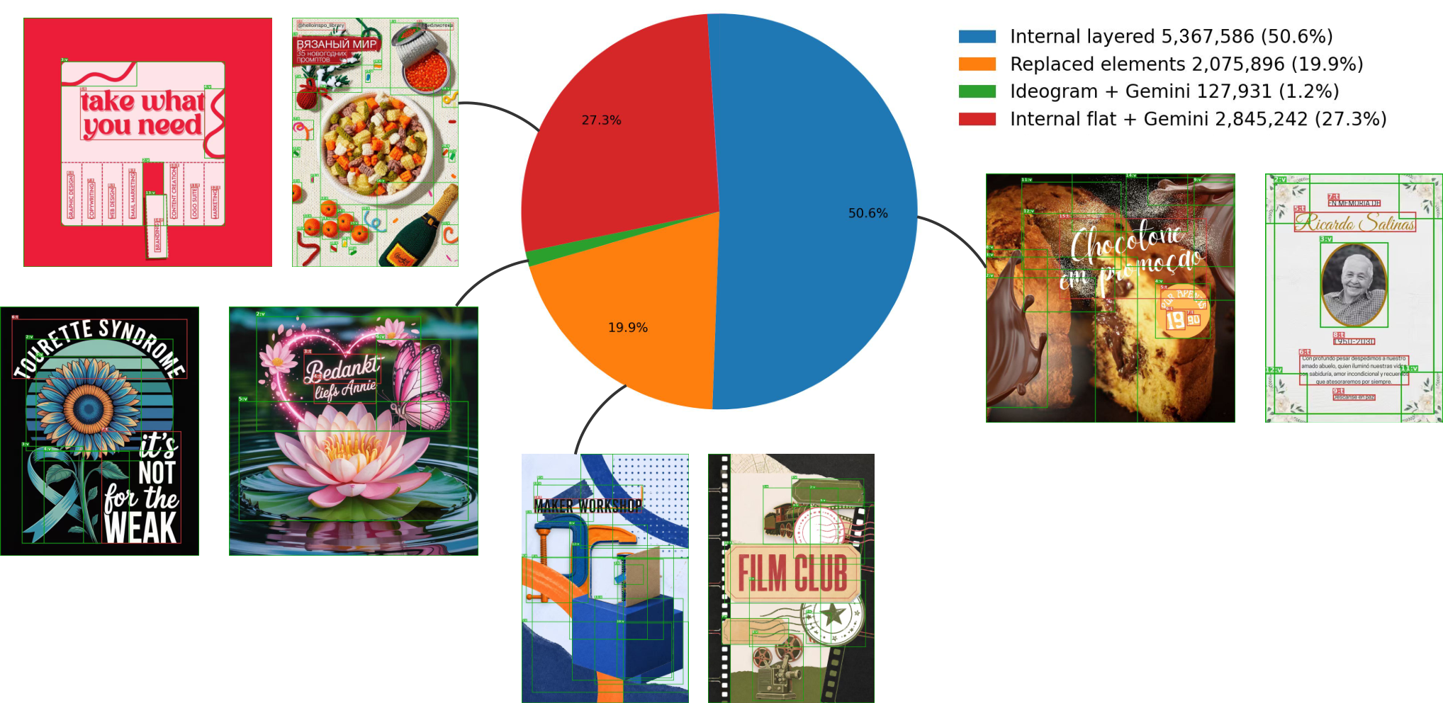
For flat designs without original layer annotations, we use Gemini-3-Pro to annotate amodal bounding boxes and compositional orders. The prompt used for annotation is provided below.

First, we mine examples that emphasize small independent elements. We train a preliminary detector on approximately $1$ M automatically annotated internal designs. We define small elements as elements whose normalized area is between $1\%$ and $5\%$ of the image area. We retain designs unused in the training of the preliminary model that contain $5$ – $10$ such small elements and for which the preliminary detector obtains a small-element recall between $0\%$ and $20\%$ . This step selects hard examples where small elements are likely to be missed or merged. It produces approximately $38$ K candidate designs.

Second, we remove designs that are likely to contain over-split annotations. We detect pairs of boxes with non-contained overlap, where two boxes intersect but neither box fully contains the other. We then group all boxes connected by such overlaps using union-find. For each connected component, we compute the number of boxes and the fill ratio, defined as the sum of box areas divided by the area of the component’s enclosing box. We filter out designs containing an overlap component with at least $10$ boxes and a fill ratio greater than $2.0$ . These cases often correspond to a single coherent element split into many overlapping parts. After filtering, we obtain $24{,}195$ high-quality designs. We use $19{,}195$ designs for RL training and $5{,}000$ designs for testing.

Appendix C DAD Training Details

We build DAD upon Qwen3-VL-2B [2]. Each element is represented by a bounding box, whose coordinates are normalized to $[0,1000]$ , and a category label indicating whether the element is text or visual. The model outputs a semicolon-delimited sequence where each element is encoded as $(x1,y1,x2,y2,c)$ , with $(x1,y1,x2,y2)$ denoting the bounding box coordinates and $c\in\{t,v\}$ the category label, e.g. , $102,35,530,210,v;45,680,980,750,t;$ . We train the model with LoRA [16] using rank $32$ and $\alpha=64$ across all linear layers. All training is conducted on NVIDIA H200 GPUs in bfloat16 precision, using AdamW [36] with $(\beta_{1},\beta_{2})=(0.9,0.95)$ and weight decay $0.1$ .

Training follows a two-stage pipeline. We first perform supervised fine-tuning (SFT) on 16 H200 GPUs for $650{,}000$ steps ( ${\sim}247$ hours) with a cosine learning rate schedule, a peak learning rate of $1\times 10^{-4}$ , a warmup ratio of $0.01$ , and a per-device batch size of $4$ . This stage uses all sources except the RL training split and the test split.

This is followed by RL using EleRPO on 8 H200 GPUs for $5{,}000$ steps ( ${\sim}20$ hours), with $16$ rollouts per image, a per-device batch size of $2$ , a cosine learning rate schedule with a peak learning rate of $5\times 10^{-7}$ , and a warmup ratio of $0.01$ . We use vLLM [23] in colocated mode for efficient rollout generation, with a sampling temperature of $0.7$ , top- $p$ of $0.9$ , and top- $k$ of $20$ . The KL regularization coefficient $\beta$ is set to $0.04$ . Following Liu et al. [34], we compute separate IoU-weighted $F_{1}$ rewards for text and visual elements, and use their average as the final reward.

Appendix D Detailed Experimental Setup for DAD Evaluation

D.1 Dataset Statistics

We evaluate DAD on the test split of DAD-10M and five external graphic design benchmarks. To ensure consistency across benchmarks, we convert all annotations into text and visual elements.

DAD-10M contains $5{,}000$ held-out test designs from our high-quality subset.

Design-Multi-Layer-Bench [49] is a multi-layer graphic design benchmark introduced by ART [49], containing $5{,}000$ designer-created works with original layered representations.

Crello [69] is a vector graphic document dataset collected from online design templates, and we use its official test split with $2{,}278$ designs.

PrismLayersPro [4] is a high-quality subset of PrismLayers [4], containing $20{,}000$ multi-layer transparent images with alpha mattes.

LICA [14] provides hierarchical component-level annotations for graphic designs, and we use the publicly released $1{,}148$ layouts and re-render images from the provided annotations.

ChartGalaxy [27] is a large-scale infographic chart dataset with structured generation specifications, and we reconstruct layered representations of $100,000$ infographic charts using its generation pipeline and sample $2{,}000$ images for evaluation. The infographic charts with layered representations are released on Huggingface.

We check each external benchmark independently against DAD-10M to ensure no duplicates. For each benchmark, we first compare exact image hashes to identify identical samples. No identical samples are identified in this step. We then perform a CLIP-based near-duplicate check. For each external benchmark, we encode both benchmark images and DAD-10M images using CLIP [51], rank all cross-dataset image pairs by cosine similarity, and manually inspect the top $1{,}000$ most similar pairs. No duplicates are found.

D.2 Baseline Implementations

For proprietary models (GPT-4o, GPT-5, GPT-5.4, GPT-5.5, Gemini-3.1-Pro), we query each model’s official API with the prompt described in Appendix B.

For open-source vision-language models (Qwen3-VL-2B/8B, InternVL3.5-2B/8B), we use vLLM for accelerated batch inference. These models receive the same structured prompt in Appendix B.

For traditional open-vocabulary detectors (GLIP-L, Detic-B, Grounding DINO-B, Florence2-L) and Rex-Omni, we use their official inference pipelines with the text prompt ["text element", "visual element"] as category queries. A confidence threshold of 0.3 is applied to GLIP-L predictions to filter low-quality detections.

All models are evaluated in a fully zero-shot setting without any task-specific fine-tuning or in-context examples.

D.3 Human Evaluation Details

We conduct human evaluation on amodal bounding-box prediction for occluded graphic elements. Figure 5 shows the web-based annotation interface. For each example, annotators are shown the visible region of a target occluded element and are asked to draw its amodal bounding box. Before annotation, annotators are given a short instruction session with examples to clarify the task. Model predictions are not shown to annotators.

Before participating, annotators read and signed an informed consent form. The consent form explains the study purpose, the annotation procedure, and the estimated study duration. It also states that participation is voluntary, that participants may stop the study at any time without providing a reason, and that they may request deletion of their data after the study. All annotation data used in our analysis are anonymized and used only for research purposes. Each annotator is compensated $\mathdollar 15$ for completing the study, which takes approximately $20$ minutes.

Appendix E Additional Results for DAD Evaluation

Tables 6, 7, 8, 9, 10, and 11 compare DAD with baselines. We evaluate the models over $3$ runs and report their mean results, except for proprietary models, which are evaluated once due to the cost of API calls. DAD achieves the best performance across all six datasets, improving overall detection quality, amodal detection quality, and ordering accuracy. It is also more efficient than proprietary baselines and comparable to open-source ones.

Table 6: Evaluation results on DAD-10M test set.

Method	$F_{1}$ @[.5:.95] $\uparrow$	IoU-weighted $F_{1}$ $\uparrow$	Occluded R@[.5:.95] $\uparrow$	POA $\uparrow$	Time (s) $\downarrow$
Proprietary
GPT-4o	4.16	7.56	5.83	1.88	2.40
GPT-5	8.99	15.99	12.59	7.14	49.02
GPT-5.4	22.41	33.37	23.31	13.94	3.16
GPT-5.5	40.89	49.46	34.26	25.42	22.01
Gemini-3.1-Pro	32.58	39.95	25.15	16.56	22.88
Open-source
GLIP-L	16.88 $\pm$ 0.78	21.04 $\pm$ 1.00	22.87 $\pm$ 6.05	-	0.34
Detic-B	4.77 $\pm$ 0.00	5.16 $\pm$ 0.00	2.47 $\pm$ 0.00	-	0.19
Grounding DINO-B	13.88 $\pm$ 0.00	15.03 $\pm$ 0.00	15.63 $\pm$ 0.00	-	0.54
Florence2-L	0.31 $\pm$ 0.44	0.37 $\pm$ 0.52	0.04 $\pm$ 0.05	-	0.54
Qwen3-VL-2B	11.75 $\pm$ 0.01	15.71 $\pm$ 0.01	6.26 $\pm$ 0.00	1.03 $\pm$ 0.00	0.86
Qwen3-VL-8B	12.90 $\pm$ 0.00	17.89 $\pm$ 0.00	10.29 $\pm$ 0.00	3.88 $\pm$ 0.00	2.19
InternVL3.5-2B	0.81 $\pm$ 0.01	1.58 $\pm$ 0.01	0.96 $\pm$ 0.01	0.05 $\pm$ 0.00	1.53
InternVL3.5-8B	4.07 $\pm$ 0.05	7.14 $\pm$ 0.11	3.98 $\pm$ 0.09	0.79 $\pm$ 0.03	1.79
Rex-Omni	31.24 $\pm$ 0.03	38.12 $\pm$ 0.04	15.41 $\pm$ 0.00	-	0.51
DAD (Ours)	72.57 $\pm$ 0.04	79.65 $\pm$ 0.03	65.35 $\pm$ 0.13	50.18 $\pm$ 0.53	0.65

Table 7: Evaluation results on Design-Multi-Layer-Bench.

Method	$F_{1}$ @[.5:.95] $\uparrow$	IoU-weighted $F_{1}$ $\uparrow$	Occluded R@[.5:.95] $\uparrow$	POA $\uparrow$
Proprietary
GPT-4o	7.67	13.95	11.89	3.38
GPT-5	13.58	24.21	21.11	8.74
GPT-5.4	38.61	54.71	46.28	25.70
GPT-5.5	61.05	70.24	61.35	34.17
Gemini-3.1-Pro	44.17	52.60	42.68	22.57
Open-source
GLIP-L	19.48 $\pm$ 4.19	24.52 $\pm$ 5.88	25.66 $\pm$ 7.33	-
Detic-B	2.98 $\pm$ 0.00	3.21 $\pm$ 0.00	2.00 $\pm$ 0.00	-
Grounding DINO-B	17.09 $\pm$ 0.00	19.09 $\pm$ 0.00	20.92 $\pm$ 0.00	-
Florence2-L	0.01 $\pm$ 0.00	0.02 $\pm$ 0.00	0.02 $\pm$ 0.00	-
Qwen3-VL-2B	29.60 $\pm$ 0.00	37.21 $\pm$ 0.00	19.36 $\pm$ 0.00	7.79 $\pm$ 0.00
Qwen3-VL-8B	38.06 $\pm$ 0.00	49.21 $\pm$ 0.00	32.80 $\pm$ 0.00	16.01 $\pm$ 0.00
InternVL3.5-2B	2.04 $\pm$ 0.00	4.12 $\pm$ 0.01	2.73 $\pm$ 0.02	0.20 $\pm$ 0.00
InternVL3.5-8B	9.95 $\pm$ 0.04	17.46 $\pm$ 0.07	11.86 $\pm$ 0.10	3.44 $\pm$ 0.03
Rex-Omni	17.79 $\pm$ 0.00	19.19 $\pm$ 0.00	13.25 $\pm$ 0.00	-
DAD (Ours)	79.52 $\pm$ 0.09	84.42 $\pm$ 0.14	71.65 $\pm$ 0.23	46.97 $\pm$ 0.22

Table 8: Evaluation results on Crello.

Method	$F_{1}$ @[.5:.95] $\uparrow$	IoU-weighted $F_{1}$ $\uparrow$	Occluded R@[.5:.95] $\uparrow$	POA $\uparrow$
Proprietary
GPT-4o	5.48	9.64	10.64	1.95
GPT-5	10.94	18.80	21.24	7.66
GPT-5.4	23.15	33.43	36.50	15.22
GPT-5.5	45.86	56.53	52.26	29.31
Gemini-3.1-Pro	34.32	42.20	36.91	18.77
Open-source
GLIP-L	16.60 $\pm$ 4.51	22.15 $\pm$ 6.30	47.45 $\pm$ 6.11	-
Detic-B	5.97 $\pm$ 0.00	6.57 $\pm$ 0.00	8.02 $\pm$ 0.00	-
Grounding DINO-B	12.29 $\pm$ 0.00	14.19 $\pm$ 0.00	21.33 $\pm$ 0.00	-
Florence2-L	0.05 $\pm$ 0.00	0.07 $\pm$ 0.00	0.08 $\pm$ 0.00	-
Qwen3-VL-2B	12.32 $\pm$ 0.00	17.17 $\pm$ 0.00	9.82 $\pm$ 0.00	2.18 $\pm$ 0.00
Qwen3-VL-8B	20.04 $\pm$ 0.00	27.33 $\pm$ 0.00	20.05 $\pm$ 0.00	8.60 $\pm$ 0.00
InternVL3.5-2B	1.64 $\pm$ 0.01	3.05 $\pm$ 0.02	2.82 $\pm$ 0.04	0.15 $\pm$ 0.00
InternVL3.5-8B	5.45 $\pm$ 0.54	9.45 $\pm$ 1.05	8.97 $\pm$ 0.38	0.86 $\pm$ 0.25
Rex-Omni	26.01 $\pm$ 0.02	33.93 $\pm$ 0.03	22.34 $\pm$ 0.02	-
DAD (Ours)	57.75 $\pm$ 0.14	68.31 $\pm$ 0.23	58.03 $\pm$ 0.20	34.89 $\pm$ 0.39

Table 9: Evaluation results on PrismLayersPro.

Method	$F_{1}$ @[.5:.95] $\uparrow$	IoU-weighted $F_{1}$ $\uparrow$	Occluded R@[.5:.95] $\uparrow$	POA $\uparrow$
Proprietary
GPT-4o	5.44	11.27	8.54	2.09
GPT-5	11.71	23.44	18.55	7.52
GPT-5.4	39.34	61.12	42.78	29.94
GPT-5.5	61.41	73.66	60.53	37.29
Gemini-3.1-Pro	40.75	48.54	37.71	22.32
Open-source
GLIP-L	24.30 $\pm$ 6.80	29.71 $\pm$ 8.83	26.45 $\pm$ 7.97	-
Detic-B	9.96 $\pm$ 0.00	10.53 $\pm$ 0.00	6.62 $\pm$ 0.00	-
Grounding DINO-B	28.28 $\pm$ 0.00	30.31 $\pm$ 0.00	32.37 $\pm$ 0.00	-
Florence2-L	0.19 $\pm$ 0.14	0.25 $\pm$ 0.17	0.27 $\pm$ 0.19	-
Qwen3-VL-2B	37.13 $\pm$ 0.00	45.19 $\pm$ 0.00	24.11 $\pm$ 0.00	11.55 $\pm$ 0.00
Qwen3-VL-8B	49.35 $\pm$ 0.02	61.04 $\pm$ 0.00	39.22 $\pm$ 0.10	26.39 $\pm$ 0.06
InternVL3.5-2B	1.19 $\pm$ 0.00	2.60 $\pm$ 0.00	1.70 $\pm$ 0.00	0.09 $\pm$ 0.00
InternVL3.5-8B	6.77 $\pm$ 0.02	13.70 $\pm$ 0.03	8.18 $\pm$ 0.03	2.11 $\pm$ 0.00
Rex-Omni	35.14 $\pm$ 0.00	38.29 $\pm$ 0.00	25.42 $\pm$ 0.00	-
DAD (Ours)	73.21 $\pm$ 0.04	78.44 $\pm$ 0.04	72.67 $\pm$ 0.04	43.87 $\pm$ 0.04

Table 10: Evaluation results on LICA.

Method	$F_{1}$ @[.5:.95] $\uparrow$	IoU-weighted $F_{1}$ $\uparrow$	Occluded R@[.5:.95] $\uparrow$	POA $\uparrow$
Proprietary
GPT-4o	4.03	7.53	6.91	2.30
GPT-5	8.83	15.99	14.88	7.94
GPT-5.4	26.10	37.07	33.23	17.96
GPT-5.5	45.92	54.95	45.10	29.53
Gemini-3.1-Pro	39.42	47.90	35.53	22.17
Open-source
GLIP-L	18.47 $\pm$ 2.88	23.54 $\pm$ 3.57	44.71 $\pm$ 7.44	-
Detic-B	4.63 $\pm$ 0.00	4.90 $\pm$ 0.00	3.63 $\pm$ 0.00	-
Grounding DINO-B	15.20 $\pm$ 0.00	16.48 $\pm$ 0.00	19.71 $\pm$ 0.00	-
Florence2-L	0.12 $\pm$ 0.00	0.15 $\pm$ 0.00	0.18 $\pm$ 0.00	-
Qwen3-VL-2B	14.79 $\pm$ 0.00	19.28 $\pm$ 0.00	10.87 $\pm$ 0.00	1.60 $\pm$ 0.00
Qwen3-VL-8B	19.22 $\pm$ 0.01	26.27 $\pm$ 0.02	17.75 $\pm$ 0.00	6.70 $\pm$ 0.00
InternVL3.5-2B	0.88 $\pm$ 0.03	1.82 $\pm$ 0.04	1.22 $\pm$ 0.04	0.11 $\pm$ 0.01
InternVL3.5-8B	6.11 $\pm$ 0.08	10.40 $\pm$ 0.08	6.98 $\pm$ 0.06	1.93 $\pm$ 0.01
Rex-Omni	28.51 $\pm$ 0.15	35.70 $\pm$ 0.22	16.37 $\pm$ 0.01	-
DAD (Ours)	71.02 $\pm$ 2.76	78.89 $\pm$ 3.35	62.67 $\pm$ 0.66	46.96 $\pm$ 1.19

Table 11: Evaluation results on ChartGalaxy.

Method	$F_{1}$ @[.5:.95] $\uparrow$	IoU-weighted $F_{1}$ $\uparrow$	Occluded R@[.5:.95] $\uparrow$	POA $\uparrow$
Proprietary
GPT-4o	0.39	0.95	0.29	0.04
GPT-5	1.30	2.84	1.46	0.42
GPT-5.4	6.08	9.47	3.99	1.70
GPT-5.5	6.85	9.42	2.98	1.12
Gemini-3.1-Pro	12.29	17.95	9.27	6.92
Open-source
GLIP-L	12.64 $\pm$ 4.45	17.71 $\pm$ 6.52	9.82 $\pm$ 4.40	-
Detic-B	5.73 $\pm$ 0.00	6.63 $\pm$ 0.00	2.01 $\pm$ 0.00	-
Grounding DINO-B	3.32 $\pm$ 0.00	3.84 $\pm$ 0.00	2.30 $\pm$ 0.00	-
Florence2-L	0.00 $\pm$ 0.00	0.00 $\pm$ 0.00	0.00 $\pm$ 0.00	-
Qwen3-VL-2B	0.08 $\pm$ 0.00	0.18 $\pm$ 0.00	0.03 $\pm$ 0.00	0.01 $\pm$ 0.00
Qwen3-VL-8B	0.99 $\pm$ 0.00	1.93 $\pm$ 0.00	0.33 $\pm$ 0.00	0.08 $\pm$ 0.00
InternVL3.5-2B	0.08 $\pm$ 0.00	0.19 $\pm$ 0.00	0.03 $\pm$ 0.00	0.00 $\pm$ 0.00
InternVL3.5-8B	0.40 $\pm$ 0.02	0.86 $\pm$ 0.02	0.22 $\pm$ 0.00	0.05 $\pm$ 0.01
Rex-Omni	6.31 $\pm$ 0.00	8.24 $\pm$ 0.00	3.16 $\pm$ 0.00	-
DAD (Ours)	32.97 $\pm$ 1.48	57.71 $\pm$ 3.62	35.76 $\pm$ 4.88	27.71 $\pm$ 6.58

As shown in Fig. 6, DAD performs robustly across diverse designs, detecting elements missed by GPT-5.5 and recovering their occluded regions.

Appendix F Detailed Experimental Setup for EleRPO Evaluation

F.1 Hyperparameters of RL Baselines

We compare EleRPO with GRPO and its extensions that incorporate finer-grained supervision, including representative policy-signal-based methods (GRPO- $\lambda$ [45], GTPO [59], and PRIME [7]) and re-rollout-based methods (VinePPO [22] and SPO [11]). Method-specific hyperparameters follow the original papers:

•

GRPO- $\lambda$ : discount factor $\lambda{=}0.99$ , return scaling $\gamma{=}1.0$ , advantage clamp threshold $-0.1$ , with both forward and backward $\lambda$ -return variants applied.
•

GTPO: entropy-weighted advantage with scaling coefficients $\alpha_{1}{=}1.0$ , $\alpha_{2}{=}0.1$ , and entropy clipped to $[0.2,0.28]$ .
•

PRIME: process reward model (PRM) learning rate $1{\times}10^{-6}$ , PRM update interval $1$ step, $K{=}4$ rollouts for PRM training, reward mixing coefficient $\beta_{\text{prime}}{=}0.05$ , and $\gamma{=}1.0$ .
•

VinePPO: $K{=}9$ re-rollouts per cutpoint, return scaling $\gamma{=}1.0$ .
•

SPO: chain mode with segment-level partitioning, $K{=}9$ Monte Carlo rollouts per segment, cutpoint threshold $0.9$ , and segment-level KL coefficient $\beta_{\text{spo}}{=}0.0001$ .

F.2 Element Order Experimental Setup

We compare three orders for predicting elements: random, left-edge order that sorts elements by their leftmost x-coordinate, and compositional order. Since random and left-edge orderings destroy the implicit compositional order conveyed by the sequence position, we augment the output format for these two variants with an explicit zero-indexed order field, resulting in the representation $(x1,y1,x2,y2,c,index)$ , e.g. , $102,35,530,210,v,3;$ . The compositional order variant retains the original format without an explicit index, as the order is naturally encoded by the sequence position.

For SFT, we train all three variants from the base Qwen3-VL-2B checkpoint for $31{,}250$ steps on 8 H200 GPUs with a learning rate of $1\times 10^{-4}$ and an effective batch size of $32$ , totaling approximately $1$ M training samples. The RL stage uses the same configuration as specified in Appendix C.

F.3 Dataset Statistics

We evaluate the generalizability of EleRPO across models and benchmarks. The benchmarks span graphic layout benchmarks with underlying layer structure, those without explicit layer structure, and natural image benchmarks. To ensure consistency across benchmarks, we convert all annotations into text and visual elements.

ChartGalaxy [27] is a large-scale infographic chart dataset with structured chart generation specifications. As described in Appendix D.1, we reconstruct layered graphic designs from these specifications and sample $5{,}000$ images for training and $2{,}000$ images for evaluation.

Crello [69] is a vector graphic document dataset as described in Appendix D.1. We use its official train/test split.

Rico [8] contains over $66$ K user interfaces collected from Android applications. Following common practice [39, 38], we split the dataset into $53$ K layouts for training and $13$ K for testing.

PosterLayout [15] is a content-aware poster layout benchmark with annotated layout elements such as text, logos, and decorative shapes. Following Zhu et al. [77], we randomly split the dataset into $8,974$ for training and $1,000$ for testing

DocLayNet [48] is a document-layout analysis dataset with human-annotated bounding boxes for document components such as text, tables, figures, titles, and lists. We use the official split with $69{,}375$ training pages and evaluate on the $6{,}489$ validation pages.

COCO [30] is a natural-image object detection benchmark. We use the train2017 split with $118{,}287$ images for training and the val2017 split with $5{,}000$ images for evaluation.

LVIS [12] is a large-vocabulary detection benchmark with long-tailed object categories. We use the official training split and evaluate on the validation split.

BDD100K [72] is a driving-scene benchmark with diverse weather and scene conditions. We use the object detection split and report results on the validation set.

Objects365 [54] is a large-scale natural-image object detection benchmark. We use the official training split and evaluate on the validation split.

Appendix G Additional Results for EleRPO Evaluation

Table 12: Additional ablation studies on key components of EleRPO.

(a) Mean Subtraction

Global	Layer
72.4	79.7

(b) Std Division

None	Global	Layer
74.0	78.6	79.7

Different cluster	None	k-means	Silhouette
78.7	79.2	79.3	79.7

We present additional ablation studies on key components of EleRPO.

Mean subtraction

Table 12(a) replaces the per-step cluster-wise mean in Eq. (3) with a single global mean computed over all $\Delta F_{1}$ values across all element positions. This leads to a performance drop, confirming that conditioning on the element position $k$ is necessary.

Standard deviation division

Table 12(b) considers two alternatives to the per-step RMS normalization in Eq. (4): 1) removing it entirely, leaving the raw mean-subtracted rewards unnormalized; and 2) replacing the per-step RMS with a global RMS pooled across all element positions. Both variants degrade performance, confirming that per-step normalization is necessary to account for the different reward variance scales at different positions.

Prefix clustering

Table 12(c) compares four strategies for forming the cluster $\mathcal{C}_{k}(i)$ in Eq. (3): 1) separate clustering, which independently clusters on $F_{1}(k{-}1)$ and $F_{1}(k)$ to form different clusters $\mathcal{C}_{k}^{-}(i)$ and $\mathcal{C}_{k}^{+}(i)$ for the two residual terms; 2) no clustering, where all rollouts share a single global mean; 3) fixed k-means with k=4, which always partitions rollouts into exactly 4 groups; and 4) our silhouette-based method. Our method performs best. The separate-clustering variant underperforms because using different clusters for the two residual terms introduces a cluster-reassignment bias. Notably, even the no-clustering variant is already competitive, suggesting that the compositional order makes a single global mean a reasonable estimate, while adaptive clustering on prefix quality further refines this estimate.

NeurIPS Paper Checklist

1.

Claims
Question: Do the main claims made in the abstract and introduction accurately reflect the paper’s contributions and scope?
Answer: [Yes]
Justification: Main claims in the abstract and introduction are backed by the task formulation, optimization method, and dataset construction in Sec. 3, and the experiments in Sec. 4.
Guidelines:
- •
  
  The answer [N/A] means that the abstract and introduction do not include the claims made in the paper.
- •
  
  The abstract and/or introduction should clearly state the claims made, including the contributions made in the paper and important assumptions and limitations. A [No] or [N/A] answer to this question will not be perceived well by the reviewers.
- •
  
  The claims made should match theoretical and experimental results, and reflect how much the results can be expected to generalize to other settings.
- •
  
  It is fine to include aspirational goals as motivation as long as it is clear that these goals are not attained by the paper.
2.

Limitations
Question: Does the paper discuss the limitations of the work performed by the authors?
Answer: [Yes]
Justification: We discuss the limitations as future work in Sec. 5.
Guidelines:
- •
  
  The answer [N/A] means that the paper has no limitation while the answer [No] means that the paper has limitations, but those are not discussed in the paper.
- •
  
  The authors are encouraged to create a separate “Limitations” section in their paper.
- •
  
  The paper should point out any strong assumptions and how robust the results are to violations of these assumptions (e.g., independence assumptions, noiseless settings, model well-specification, asymptotic approximations only holding locally). The authors should reflect on how these assumptions might be violated in practice and what the implications would be.
- •
  
  The authors should reflect on the scope of the claims made, e.g., if the approach was only tested on a few datasets or with a few runs. In general, empirical results often depend on implicit assumptions, which should be articulated.
- •
  
  The authors should reflect on the factors that influence the performance of the approach. For example, a facial recognition algorithm may perform poorly when image resolution is low or images are taken in low lighting. Or a speech-to-text system might not be used reliably to provide closed captions for online lectures because it fails to handle technical jargon.
- •
  
  The authors should discuss the computational efficiency of the proposed algorithms and how they scale with dataset size.
- •
  
  If applicable, the authors should discuss possible limitations of their approach to address problems of privacy and fairness.
- •
  
  While the authors might fear that complete honesty about limitations might be used by reviewers as grounds for rejection, a worse outcome might be that reviewers discover limitations that aren’t acknowledged in the paper. The authors should use their best judgment and recognize that individual actions in favor of transparency play an important role in developing norms that preserve the integrity of the community. Reviewers will be specifically instructed to not penalize honesty concerning limitations.
3.

Theory assumptions and proofs
Question: For each theoretical result, does the paper provide the full set of assumptions and a complete (and correct) proof?
Answer: [Yes]
Justification: We provide the assumptions in Sec. 3.2.1 and the complete proof in Appendix A.
Guidelines:
- •
  
  The answer [N/A] means that the paper does not include theoretical results.
- •
  
  All the theorems, formulas, and proofs in the paper should be numbered and cross-referenced.
- •
  
  All assumptions should be clearly stated or referenced in the statement of any theorems.
- •
  
  The proofs can either appear in the main paper or the supplemental material, but if they appear in the supplemental material, the authors are encouraged to provide a short proof sketch to provide intuition.
- •
  
  Inversely, any informal proof provided in the core of the paper should be complemented by formal proofs provided in appendix or supplemental material.
- •
  
  Theorems and Lemmas that the proof relies upon should be properly referenced.
4.

Experimental result reproducibility
Question: Does the paper fully disclose all the information needed to reproduce the main experimental results of the paper to the extent that it affects the main claims and/or conclusions of the paper (regardless of whether the code and data are provided or not)?
Answer: [Yes]
Justification: We describe how we build our model in Sec. 3, and provide experimental details in Appendices C, D and F.
Guidelines:
- •
  
  The answer [N/A] means that the paper does not include experiments.
- •
  
  If the paper includes experiments, a [No] answer to this question will not be perceived well by the reviewers: Making the paper reproducible is important, regardless of whether the code and data are provided or not.
- •
  
  If the contribution is a dataset and/or model, the authors should describe the steps taken to make their results reproducible or verifiable.
- •
  
  Depending on the contribution, reproducibility can be accomplished in various ways. For example, if the contribution is a novel architecture, describing the architecture fully might suffice, or if the contribution is a specific model and empirical evaluation, it may be necessary to either make it possible for others to replicate the model with the same dataset, or provide access to the model. In general. releasing code and data is often one good way to accomplish this, but reproducibility can also be provided via detailed instructions for how to replicate the results, access to a hosted model (e.g., in the case of a large language model), releasing of a model checkpoint, or other means that are appropriate to the research performed.
- •
  While NeurIPS does not require releasing code, the conference does require all submissions to provide some reasonable avenue for reproducibility, which may depend on the nature of the contribution. For example
  1. (a)
    
    If the contribution is primarily a new algorithm, the paper should make it clear how to reproduce that algorithm.
  2. (b)
    
    If the contribution is primarily a new model architecture, the paper should describe the architecture clearly and fully.
  3. (c)
    
    If the contribution is a new model (e.g., a large language model), then there should either be a way to access this model for reproducing the results or a way to reproduce the model (e.g., with an open-source dataset or instructions for how to construct the dataset).
  4. (d)
    
    We recognize that reproducibility may be tricky in some cases, in which case authors are welcome to describe the particular way they provide for reproducibility. In the case of closed-source models, it may be that access to the model is limited in some way (e.g., to registered users), but it should be possible for other researchers to have some path to reproducing or verifying the results.
5.

Open access to data and code
Question: Does the paper provide open access to the data and code, with sufficient instructions to faithfully reproduce the main experimental results, as described in supplemental material?
Answer: [Yes]
Justification: We have released our code and $100,000$ designs in our dataset, and provided the links in the abstract.
Guidelines:
- •
  
  The answer [N/A] means that paper does not include experiments requiring code.
- •
  
  Please see the NeurIPS code and data submission guidelines (https://neurips.cc/public/guides/CodeSubmissionPolicy) for more details.
- •
  
  While we encourage the release of code and data, we understand that this might not be possible, so [No] is an acceptable answer. Papers cannot be rejected simply for not including code, unless this is central to the contribution (e.g., for a new open-source benchmark).
- •
  
  The instructions should contain the exact command and environment needed to run to reproduce the results. See the NeurIPS code and data submission guidelines (https://neurips.cc/public/guides/CodeSubmissionPolicy) for more details.
- •
  
  The authors should provide instructions on data access and preparation, including how to access the raw data, preprocessed data, intermediate data, and generated data, etc.
- •
  
  The authors should provide scripts to reproduce all experimental results for the new proposed method and baselines. If only a subset of experiments are reproducible, they should state which ones are omitted from the script and why.
- •
  
  At submission time, to preserve anonymity, the authors should release anonymized versions (if applicable).
- •
  
  Providing as much information as possible in supplemental material (appended to the paper) is recommended, but including URLs to data and code is permitted.
6.

Experimental setting/details
Question: Does the paper specify all the training and test details (e.g., data splits, hyperparameters, how they were chosen, type of optimizer) necessary to understand the results?
Answer: [Yes]
Justification: We have provided details for the experimental setup in Appendices C, D, and F.
Guidelines:
- •
  
  The answer [N/A] means that the paper does not include experiments.
- •
  
  The experimental setting should be presented in the core of the paper to a level of detail that is necessary to appreciate the results and make sense of them.
- •
  
  The full details can be provided either with the code, in appendix, or as supplemental material.
7.

Experiment statistical significance
Question: Does the paper report error bars suitably and correctly defined or other appropriate information about the statistical significance of the experiments?
Answer: [Yes]
Justification: We report the variance for the evaluation of object detection models in Appendix E.
Guidelines:
- •
  
  The answer [N/A] means that the paper does not include experiments.
- •
  
  The authors should answer [Yes] if the results are accompanied by error bars, confidence intervals, or statistical significance tests, at least for the experiments that support the main claims of the paper.
- •
  
  The factors of variability that the error bars are capturing should be clearly stated (for example, train/test split, initialization, random drawing of some parameter, or overall run with given experimental conditions).
- •
  
  The method for calculating the error bars should be explained (closed form formula, call to a library function, bootstrap, etc.)
- •
  
  The assumptions made should be given (e.g., Normally distributed errors).
- •
  
  It should be clear whether the error bar is the standard deviation or the standard error of the mean.
- •
  
  It is OK to report 1-sigma error bars, but one should state it. The authors should preferably report a 2-sigma error bar than state that they have a 96% CI, if the hypothesis of Normality of errors is not verified.
- •
  
  For asymmetric distributions, the authors should be careful not to show in tables or figures symmetric error bars that would yield results that are out of range (e.g., negative error rates).
- •
  
  If error bars are reported in tables or plots, the authors should explain in the text how they were calculated and reference the corresponding figures or tables in the text.
8.

Experiments compute resources
Question: For each experiment, does the paper provide sufficient information on the computer resources (type of compute workers, memory, time of execution) needed to reproduce the experiments?
Answer: [Yes]
Justification: We report the compute resources to conduct our experiments in Appendix C.
Guidelines:
- •
  
  The answer [N/A] means that the paper does not include experiments.
- •
  
  The paper should indicate the type of compute workers CPU or GPU, internal cluster, or cloud provider, including relevant memory and storage.
- •
  
  The paper should provide the amount of compute required for each of the individual experimental runs as well as estimate the total compute.
- •
  
  The paper should disclose whether the full research project required more compute than the experiments reported in the paper (e.g., preliminary or failed experiments that didn’t make it into the paper).
9.

Code of ethics
Question: Does the research conducted in the paper conform, in every respect, with the NeurIPS Code of Ethics https://neurips.cc/public/EthicsGuidelines?
Answer: [Yes]
Justification: We have read the NeurIPS Code of Ethics and made sure that the paper conforms to it.
Guidelines:
- •
  
  The answer [N/A] means that the authors have not reviewed the NeurIPS Code of Ethics.
- •
  
  If the authors answer [No] , they should explain the special circumstances that require a deviation from the Code of Ethics.
- •
  
  The authors should make sure to preserve anonymity (e.g., if there is a special consideration due to laws or regulations in their jurisdiction).
10.

Broader impacts
Question: Does the paper discuss both potential positive societal impacts and negative societal impacts of the work performed?
Answer: [N/A]
Justification: There are no obvious paths that this work leads to potential negative societal impacts.
Guidelines:
- •
  
  The answer [N/A] means that there is no societal impact of the work performed.
- •
  
  If the authors answer [N/A] or [No] , they should explain why their work has no societal impact or why the paper does not address societal impact.
- •
  
  Examples of negative societal impacts include potential malicious or unintended uses (e.g., disinformation, generating fake profiles, surveillance), fairness considerations (e.g., deployment of technologies that could make decisions that unfairly impact specific groups), privacy considerations, and security considerations.
- •
  
  The conference expects that many papers will be foundational research and not tied to particular applications, let alone deployments. However, if there is a direct path to any negative applications, the authors should point it out. For example, it is legitimate to point out that an improvement in the quality of generative models could be used to generate Deepfakes for disinformation. On the other hand, it is not needed to point out that a generic algorithm for optimizing neural networks could enable people to train models that generate Deepfakes faster.
- •
  
  The authors should consider possible harms that could arise when the technology is being used as intended and functioning correctly, harms that could arise when the technology is being used as intended but gives incorrect results, and harms following from (intentional or unintentional) misuse of the technology.
- •
  
  If there are negative societal impacts, the authors could also discuss possible mitigation strategies (e.g., gated release of models, providing defenses in addition to attacks, mechanisms for monitoring misuse, mechanisms to monitor how a system learns from feedback over time, improving the efficiency and accessibility of ML).
11.

Safeguards
Question: Does the paper describe safeguards that have been put in place for responsible release of data or models that have a high risk for misuse (e.g., pre-trained language models, image generators, or scraped datasets)?
Answer: [N/A]
Justification: We do not foresee any high risk for misuse of this work.
Guidelines:
- •
  
  The answer [N/A] means that the paper poses no such risks.
- •
  
  Released models that have a high risk for misuse or dual-use should be released with necessary safeguards to allow for controlled use of the model, for example by requiring that users adhere to usage guidelines or restrictions to access the model or implementing safety filters.
- •
  
  Datasets that have been scraped from the Internet could pose safety risks. The authors should describe how they avoided releasing unsafe images.
- •
  
  We recognize that providing effective safeguards is challenging, and many papers do not require this, but we encourage authors to take this into account and make a best faith effort.
12.

Licenses for existing assets
Question: Are the creators or original owners of assets (e.g., code, data, models), used in the paper, properly credited and are the license and terms of use explicitly mentioned and properly respected?
Answer: [Yes]
Justification: We credit the original owners of assets and mention the terms of use in Appendix B.
Guidelines:
- •
  
  The answer [N/A] means that the paper does not use existing assets.
- •
  
  The authors should cite the original paper that produced the code package or dataset.
- •
  
  The authors should state which version of the asset is used and, if possible, include a URL.
- •
  
  The name of the license (e.g., CC-BY 4.0) should be included for each asset.
- •
  
  For scraped data from a particular source (e.g., website), the copyright and terms of service of that source should be provided.
- •
  
  If assets are released, the license, copyright information, and terms of use in the package should be provided. For popular datasets, paperswithcode.com/datasets has curated licenses for some datasets. Their licensing guide can help determine the license of a dataset.
- •
  
  For existing datasets that are re-packaged, both the original license and the license of the derived asset (if it has changed) should be provided.
- •
  
  If this information is not available online, the authors are encouraged to reach out to the asset’s creators.
13.

New assets
Question: Are new assets introduced in the paper well documented and is the documentation provided alongside the assets?
Answer: [Yes]
Justification: We host our dataset on Huggingface and provide detailed documentation. The Huggingface link to the dataset is provided in the abstract.
Guidelines:
- •
  
  The answer [N/A] means that the paper does not release new assets.
- •
  
  Researchers should communicate the details of the dataset/code/model as part of their submissions via structured templates. This includes details about training, license, limitations, etc.
- •
  
  The paper should discuss whether and how consent was obtained from people whose asset is used.
- •
  
  At submission time, remember to anonymize your assets (if applicable). You can either create an anonymized URL or include an anonymized zip file.
14.

Crowdsourcing and research with human subjects
Question: For crowdsourcing experiments and research with human subjects, does the paper include the full text of instructions given to participants and screenshots, if applicable, as well as details about compensation (if any)?
Answer: [Yes]
Justification: We provide the screenshot of the web-based prototype and compensation details in Appendix D.3.
Guidelines:
- •
  
  The answer [N/A] means that the paper does not involve crowdsourcing nor research with human subjects.
- •
  
  Including this information in the supplemental material is fine, but if the main contribution of the paper involves human subjects, then as much detail as possible should be included in the main paper.
- •
  
  According to the NeurIPS Code of Ethics, workers involved in data collection, curation, or other labor should be paid at least the minimum wage in the country of the data collector.
15.

Institutional review board (IRB) approvals or equivalent for research with human subjects
Question: Does the paper describe potential risks incurred by study participants, whether such risks were disclosed to the subjects, and whether Institutional Review Board (IRB) approvals (or an equivalent approval/review based on the requirements of your country or institution) were obtained?
Answer: [Yes]
Justification: The paper describes the human evaluation protocol in Appendix D.3, including how consent was received from participants. The study involves only a simple, low-risk annotation task lasting approximately 20 minutes and has received IRB approval.
Guidelines:
- •
  
  The answer [N/A] means that the paper does not involve crowdsourcing nor research with human subjects.
- •
  
  Depending on the country in which research is conducted, IRB approval (or equivalent) may be required for any human subjects research. If you obtained IRB approval, you should clearly state this in the paper.
- •
  
  We recognize that the procedures for this may vary significantly between institutions and locations, and we expect authors to adhere to the NeurIPS Code of Ethics and the guidelines for their institution.
- •
  
  For initial submissions, do not include any information that would break anonymity (if applicable), such as the institution conducting the review.
16.

Declaration of LLM usage
Question: Does the paper describe the usage of LLMs if it is an important, original, or non-standard component of the core methods in this research? Note that if the LLM is used only for writing, editing, or formatting purposes and does not impact the core methodology, scientific rigor, or originality of the research, declaration is not required.
Answer: [Yes]
Justification: We describe how we build our detection model on top of a VLM, Qwen3-VL-2B, in Sec. 3.
Guidelines:
- •
  
  The answer [N/A] means that the core method development in this research does not involve LLMs as any important, original, or non-standard components.
- •
  
  Please refer to our LLM policy in the NeurIPS handbook for what should or should not be described.

Detect Anything in Graphic Design: Element-Level Rewards for Autoregressive Detection

Abstract

1 Introduction

2 Related Work

Autoregressive Object Detection

Reward Design for RL Post-Training

3 Method

3.1 Task Formulation

3.2 Element Relative Policy Optimization

3.2.1 Element-Level Reward via Martingale Difference Decomposition

3.2.2 Advantage Estimation from Sampled Rollouts

3.3 Dataset Construction

Data collection

Data selection

3.4 Implementation Details

4 Experiments

4.1 Performance of DAD

4.1.1 Comparison with State-of-the-Art

Datasets

Evaluation metrics

Baselines

Results

4.1.2 Human Evaluation on Amodal Detection

Experimental setup

Results

4.1.3 Application to Image-to-Layer Decomposition

Experimental setup

Results

4.2 Effectiveness of EleRPO

4.2.1 Comparison with Existing Methods

Experimental setup

Results

4.2.2 Ablation Studies

Reward causality

Advantage combination

Element order

4.2.3 Generalizability of EleRPO

Experimental setup

Results

5 Conclusion

References

Appendix A Theoretical Derivations for EleRPO

A.1 Proof of the Martingale Difference Decomposition

Completeness

Causality

Unbiasedness

A.2 Derivation of the Element-Level Reward Estimator and Justification for Cluster Reuse

A.3 Empirical Validation of the Prefix-Clustering Approximation

A.4 Magnitude Analysis of the Element-Level Reward

Appendix B DAD-10M Dataset Construction

Appendix C DAD Training Details

Appendix D Detailed Experimental Setup for DAD Evaluation

D.1 Dataset Statistics

D.2 Baseline Implementations

D.3 Human Evaluation Details

Appendix E Additional Results for DAD Evaluation

Appendix F Detailed Experimental Setup for EleRPO Evaluation

F.1 Hyperparameters of RL Baselines

F.2 Element Order Experimental Setup

F.3 Dataset Statistics

Appendix G Additional Results for EleRPO Evaluation

Mean subtraction

Standard deviation division

Prefix clustering

NeurIPS Paper Checklist

Detect Anything in Graphic Design:
Element-Level Rewards for Autoregressive Detection