VERPO:
Verified Evidence Regularized Policy Optimization

Haijiang Li¹, Chengyu Lv², Yi Zhang¹, Zhibing Zhang³, Rui Qian⁴, Yuchen Zhang⁵, Xiaofan Zhang⁶, Mingshan Wang⁶, Xiaofei Jing⁶, Yu Tong⁶, Cangqi Zhou⁵ ¹Independent ²Tongji University ³Nanjing University ⁴Fudan University ⁵Nanjing University of Science and Technology ⁶Xiaohongshu Email: hj523hj@163.com, 2532065@tongji.edu.cn, myjoeycheung@gmail.com, 602026710049@smail.nju.edu.cn, qianruii@gmail.com, zhangyc811@njust.edu.cn, fantasyjxf@gmail.com, yutchina02@gmail.com, cqzhou@njust.edu.cn.

Abstract

Verifiable outcome rewards guide language-model post-training, but sequence-level advantages do not identify which token-level decisions should be preserved or revised. Evidence-conditioned Teachers provide denser supervision by replaying sampled trajectories with privileged feedback. Yet indiscriminate imitation risks transferring formatting or reasoning-style shifts that do not support task success. We introduce VERPO, a Verified Evidence Regularized Policy Optimization framework that treats evidence as a proposal for policy correction while retaining the outcome objective. It separates evidence-free reference restoration from signed token-level evidence corrections. Fisher Evidence Contrast attenuates corrections along an estimated evidence-presence direction. A stopped token-wise ZPD controller scales acceptance according to local reward alignment and Fisher movement cost, while the reference channel remains independent of acceptance. Across five scientific-reasoning and tool-use tasks, the best variant on each backbone exceeds the strongest compared baseline in average score. The averages rise from 0.6826 to 0.6857 on Qwen3-4B, from 0.6895 to 0.7058 on Qwen3-8B, and from 0.4751 to 0.5657 on Llama-3.2-1B.

1 Introduction

Outcome-based policy optimization with verifiable rewards has become a central approach for improving the reasoning behavior of language models (Shao et al., 2024; DeepSeek-AI, 2025; Yu et al., 2025). In reinforcement learning with verifiable rewards (RLVR), task success can be checked automatically, allowing policy updates to be grounded in reliable outcome-level feedback. Group Relative Policy Optimization (GRPO) (Shao et al., 2024) derives group-relative advantages from multiple on-policy rollouts and uses them to reinforce or suppress complete responses. This signal is attractive because it is directly tied to final task success. However, GRPO-style methods apply the resulting sequence-level advantage uniformly across all response tokens. This coarse credit assignment reinforces or penalizes an entire response without identifying which local decisions should be preserved, reinforced, or revised.

Evidence-conditioned self-distillation offers a complementary source of supervision. By replaying sampled trajectories with privileged feedback, a self-Teacher can provide dense token-level guidance without requiring the deployed Student to access that evidence (Hübotter et al., 2026). This addresses the sparsity of outcome rewards, but it introduces a different problem: a Teacher–Student discrepancy is not automatically a task-improving correction. Naively imitating the evidence-conditioned Teacher distribution can transfer evidence-induced artifacts, including formatting, confidence, verbosity, or reasoning-style preferences, rather than only task-relevant improvements (Lazaridis et al., 2026; Harne et al., 2026). Such shifts can destabilize learning when they are not aligned with verifiable task success (Kaur et al., 2026; Harne et al., 2026).

These observations suggest that the central challenge is not simply how to combine an RL loss with a distillation loss. Rather, a useful method must separate three roles that are usually entangled: the outcome-based criterion that defines task improvement, the evidence-induced direction that proposes a local policy change, and the decision of whether that change is worth accepting at a particular token. This leads to the question:

Can evidence provide dense guidance for outcome-based optimization while remaining subordinate to the verifiable reward objective?

We introduce VERPO, a Verified Evidence-Regularized Policy Optimization framework that treats evidence as a proposal for policy correction rather than as a replacement for the outcome objective. VERPO decomposes Teacher guidance into an evidence-free reference term, which preserves reference behavior, and a signed evidence-induced correction, which proposes how the policy should move at each token. After this decomposition, VERPO uses a stopped token-wise controller to decide how much of each correction to accept. The controller compares the correction’s alignment with the local GRPO update direction against its Fisher movement cost, so evidence guidance is strongest where it is reward-aligned and inexpensive to incorporate.

Refer to caption — Figure 1: Left: Verifiable RL relies on sparse outcome rewards, requiring trial-and-error exploration with many failed attempts. Right: VERPO augments the outcome signal with selective local corrections and adaptive guidance, providing targeted supervision along the trajectory while preserving reward-based improvement.

Figure 1 illustrates this motivation. The left panel depicts standard verifiable RL as trial-and-error exploration driven by sparse outcome rewards: the model receives reliable feedback only after a full response is generated, leaving many intermediate reasoning decisions unsupported. The right panel shows the VERPO view: evidence supplies local correction proposals along the trajectory, while the controller adaptively scales those proposals instead of applying them uniformly. Thus, VERPO retains reward-based optimization as the anchor but adds targeted supervision at positions where evidence is justified.

Table 1 further summarizes the distinction between VERPO and representative alternatives. GRPO (Shao et al., 2024) uses outcome rewards and requires no external Teacher, but lacks dense token guidance and token-wise selectivity. SDPO (Hübotter et al., 2026) provides dense self-distillation guidance without an external Teacher, but does not anchor corrections to verifiable rewards and applies Teacher preferences without reward-verified token-level acceptance. VERPO combines the strengths of both: it preserves the outcome reward signal, obtains dense token-level evidence guidance, and introduces reward-verified, token-wise selective corrections. This comparison highlights that VERPO is not merely a weighted sum of GRPO and self-distillation; it changes the role of evidence from a supervision target into a locally controlled correction proposal.

Table 1: GRPO, SDPO, VERPO Comparison

	GRPO	SDPO	VERPO
Outcome Reward	$\checkmark$	$\times$	$\checkmark$
Dense Token Guidance	$\times$	$\checkmark$	$\checkmark$
No External Teacher	$\checkmark$	$\checkmark$	$\checkmark$
Reward-Verified Correction	$\times$	$\times$	$\checkmark$
Token-Wise Selectivity	$\times$	$\times$	$\checkmark$

We instantiate VERPO with multiple evidence-direction constructions. The Fix construction (Hübotter et al., 2026) compares an evidence-conditioned Teacher with an evidence-free Teacher, while the Contrastive (CTR) construction (Pan et al., 2026) compares Teacher distributions under correct and incorrect evidence. We further introduce Fisher Evidence Contrast (FEC), which projects out nuisance shifts associated with the mere presence of privileged evidence. The resulting correction can be used through two update paths: it can scale the evidence-distillation loss, modulate the token-level policy advantage, or enter both paths through the same stopped controller.

We evaluate VERPO on five scientific-reasoning and tool-use tasks with Qwen3-4B (Yang et al., 2025), Qwen3-8B (Yang et al., 2025), and Llama-3.2-1B (Meta, 2024). The best VERPO variant on each backbone exceeds the strongest baseline with complete noncollapsed results in five-task average. The averages rise from 0.6826 to 0.6857 on Qwen3-4B, from 0.6895 to 0.7058 on Qwen3-8B, and from 0.4751 to 0.5657 on Llama-3.2-1B. These are point estimates without uncertainty across seeds. Diagnostic analyses describe task-dependent acceptance consistent with the controller’s use of local reward alignment and Fisher movement cost.

Our contributions are as follows:

•

We formulate evidence-conditioned self-distillation for RLVR as a separation problem, distinguishing evidence-free reference preservation from signed evidence-induced policy correction.
•

We propose a stopped token-wise controller that accepts and scales each evidence correction according to local reward alignment and Fisher movement cost.
•

We instantiate multiple evidence-direction constructions, including Fisher Evidence Contrast, which removes nuisance shifts caused by evidence presence.
•

We report higher five-task averages than GRPO (Shao et al., 2024), SDPO (Hübotter et al., 2026), and SRPO (Li et al., 2026) on three backbones, and analyze when and where token-level corrections are applied.

2 Related Work

RLVR and fine-grained credit assignment.

Reinforcement learning with verifiable rewards (RLVR) optimizes language models using automatically checkable outcome rewards. Critic-free methods such as GRPO (Shao et al., 2024) replace traditional actor–critic value estimates with group-relative advantages computed from multiple on-policy responses. DeepSeek-R1 (DeepSeek-AI, 2025) and DAPO (Yu et al., 2025) use related group-relative updates for scalable RLVR. These sequence-level advantages are shared across response tokens, obscuring which local decisions caused the outcome. Process supervision obtains finer-grained signals through human-annotated step verification in Let’s Verify Step by Step (Lightman et al., 2024), automatically constructed labels in Math-Shepherd (Wang et al., 2024), and outcome-derived progress estimates in Rewarding Progress (Setlur et al., 2025). Such approaches require human annotations or automatically generated process targets together with a learned verifier, whose local preferences need not match the verifiable sequence-level objective. VERPO retains the outcome-derived GRPO advantage as the task-level anchor and uses privileged Teacher replay to propose token-level corrections, accepting them only when they align with the local reward direction at justified Fisher movement cost.

On-policy distillation and self-distillation.

Knowledge distillation transfers a teacher’s predictive distribution to a student (Hinton et al., 2015). On-policy distillation reduces off-policy distribution shift by supervising student-generated trajectories with an external teacher (Agarwal et al., 2023). MiniLLM develops a related distribution-matching formulation for language-model distillation (Gu et al., 2023). OPSD removes the external teacher by conditioning the same model on privileged solutions (Zhao et al., 2026a), and SDPO constructs a feedback-conditioned self-teacher for dense token-level supervision (Hübotter et al., 2026). SRPO (Li et al., 2026) anchors self-distillation to verifiable outcomes through sample-level routing. EviSD (Xie et al., 2026) applies reward-anchored modulation to evidence-conditioned search actions. These methods do not jointly separate evidence-free reference retention from signed evidence-induced change, and they do not decide whether an individual correction is worth applying at its local policy cost. VERPO addresses this control gap with a stopped token-wise ZPD controller that accepts and scales each correction according to its alignment with the local GRPO direction and its Fisher movement cost.

Selective and contrastive privileged supervision.

Empirical studies show that privileged supervision is not uniformly reliable across rollouts or tokens (Armandpour et al., 2026; Harne et al., 2026; Lazaridis et al., 2026; Zhao et al., 2026b; Kaur et al., 2026; Jiang et al., 2026). Teacher guidance is better aligned on incorrect than on already-correct trajectories (Armandpour et al., 2026), while privileged conditioning can bias the Teacher toward a particular reference trajectory rather than toward correctness in general (Harne et al., 2026), induce behavior unrelated to the intended correction (Lazaridis et al., 2026), overwrite valid reasoning prefixes (Zhao et al., 2026b), suppress verification and backtracking in thinking models (Kaur et al., 2026), or amplify weakly input-grounded signals (Jiang et al., 2026). CEPO (Heakl et al., 2026) exploits correct-wrong evidence for contrastive token credit, while OCSD (Yang et al., 2026) uses structurally matched privileged and ablated replay views to remove replay-scaffold effects in agentic RL. These contrastive constructions reduce shared effects between privileged branches, but a Teacher difference can still contain a component caused by the mere presence of privileged evidence. Such a component can leak evidence-specific style, confidence, or formatting into the Student without improving task success. VERPO’s Fisher Evidence Contrast (FEC) estimates this evidence-presence direction and projects it out of the task contrast under the local Fisher metric, reducing privileged-context leakage before the resulting correction is applied.

3 Method

VERPO separates reference restoration, evidence correction, and token-wise acceptance. An evidence-free Teacher anchors the Actor’s behavior, Teacher comparisons propose a signed correction, and a stopped ZPD weight controls its contribution to training. The weight scales an evidence correction derived from OPSD (Zhao et al., 2026a) or modulates the GRPO (Shao et al., 2024) advantage. We develop the method under forward-KL geometry, denoted FKL. Appendix C.3 derives the reverse-KL counterpart, denoted RKL.

3.1 Overview of VERPO

VERPO separates evidence correction from token-wise acceptance. Teacher comparisons propose a signed correction, and ZPD controls its strength using local reward alignment and Fisher movement cost. A separate evidence-free reference channel anchors the Actor’s behavior.

Figure 2 summarizes the four-stage training pipeline:

•

Stage 1: Rollout Sampling and Outcome Signal. The Actor samples response groups. Verifier rewards determine the group-relative advantage $\widehat{A}_{i}$ used by GRPO (Shao et al., 2024).
•

Stage 2: Token-Level Evidence Correction. The frozen Teacher replays sampled prefixes under different evidence contexts. Fix (Hübotter et al., 2026), Contrastive (Pan et al., 2026), or FEC constructs the signed correction, as defined in Section 3.4.
•

Stage 3: ZPD Weight Estimation. Reward alignment and Fisher movement cost determine the stopped acceptance weight $w_{i,t}^{*}$ for each eligible token, as derived in Section 3.3.
•

Stage 4: Two-Path Policy Update. The weight either scales the evidence correction or modulates the GRPO (Shao et al., 2024) advantage. Section 3.5 defines both update paths.

3.2 FKL Evidence Direction and OPSD Decomposition

To control reference restoration and evidence correction separately, we decompose the forward-KL Teacher objective along a path between two Teacher endpoints. In particular, we isolate the signed evidence correction from the base restoration term, allowing ZPD to scale the correction independently of the reference channel.

Let $q_{b}$ and $q_{e}$ denote the base and evidence-enriched Teacher distributions, respectively. The base endpoint uses no evidence or incorrect evidence, while the enriched endpoint uses correct evidence in our experiments. The Actor distribution $p_{i,t}=\pi_{\theta}(\cdot\mid x_{i},y_{i,<t})$ uses the original prompt and sampled prefix. We suppress the response and token indices when describing a single Teacher comparison. Section 3.4 specifies the endpoint constructions. We hold the Teacher distributions and $w$ fixed during Actor differentiation and assume positive probability support over the vocabulary $\mathcal{V}$ . To vary the strength of the evidence-induced change, we define the signed probability displacement and arithmetic path as

\Delta=q_{e}-q_{b},\qquad q_{w}^{\mathrm{FKL}}=q_{b}+w\Delta,\qquad 0\leq w\leq 1.

(1)

The displacement $\Delta$ records which vocabulary items gain or lose probability under the enriched Teacher. The path interpolates from $q_{b}$ at $w=0$ to $q_{e}$ at $w=1$ , preserving a normalized distribution throughout. Expanding the forward-KL objective along this path separates base restoration from the evidence-induced correction:

\mathrm{KL}(q_{w}^{\mathrm{FKL}}\|p)=\mathrm{KL}(q_{b}\|p)-w\sum_{v\in\mathcal{V}}\Delta(v)\log p(v)+C(q_{w}^{\mathrm{FKL}},q_{b}),

(2)

The first term pulls the Actor toward $q_{b}$ . The second term contributes the signed correction $w\Delta$ to the negative logit gradient, while the remainder $C$ depends only on the fixed Teacher path and contributes no Actor gradient. Appendix C.2 derives the identity and exact logit gradient in Equations (C.5) and (C.6).

This separation lets us choose the reference anchor independently of the evidence endpoints. In the training objective, we use the evidence-free Teacher $q_{i,t}^{\mathrm{ref}}$ for restoration, even when the correction uses an incorrect-evidence base. Averaging over valid response tokens gives

\mathcal{L}_{\mathrm{ref}}^{\mathrm{FKL}}=\frac{1}{N}\sum_{i,t}a_{i,t}\mathrm{KL}(q_{i,t}^{\mathrm{ref}}\|p_{i,t}),

(3)

Here $a_{i,t}$ selects valid response tokens and $N$ counts them. This reference loss remains active independently of evidence acceptance. We then apply the signed correction only to tokens selected by the evidence mask $m_{i,t}$ and scale each contribution by its stopped weight $w_{i,t}$ :

\mathcal{L}_{\mathrm{OPSD}}^{\mathrm{FKL}}(w)=-\frac{1}{Z_{\mathrm{evi}}}\sum_{i,t}m_{i,t}w_{i,t}\sum_{v\in\mathcal{V}}\Delta_{i,t}(v)\log p_{i,t}(v).

(4)

The normalizer $Z_{\mathrm{evi}}$ counts eligible tokens with a floor of one, so reducing acceptance weights reduces the correction strength without renormalizing it away. A zero weight removes that token’s evidence correction while retaining its reference loss. The resulting objective therefore controls reference retention and evidence acceptance through separate channels.

These definitions use full-vocabulary distributions. The implementation uses a finite-support approximation for the Teacher evidence terms. Appendix F.4 specifies support construction, normalization, and the approximation boundary. With the correction defined, Section 3.3 determines its token-wise weight from local reward alignment and policy movement cost.

3.3 Token-Wise ZPD Controller

To determine how strongly to apply each evidence correction, we compare its local reward alignment with its Fisher movement cost. In particular, we construct a stopped token-wise weight $w_{i,t}^{*}$ that rejects corrections opposing the local GRPO (Shao et al., 2024) direction and is nonincreasing with movement cost at fixed alignment benefit.

To derive a practical acceptance rule, we first consider the ideal improvement in the RL objective $J_{\mathrm{RL}}$ from applying a fraction $w$ of one token’s correction. Let $\theta_{\mathrm{base}}$ denote a hypothetical Actor state after the GRPO (Shao et al., 2024) and reference updates. This state serves only as a reference for the derivation. The training algorithm updates the Actor through a joint loss and reserves $\bar{\theta}$ for the EMA Teacher. For Actor logits $z_{i,t}$ , define the logit Jacobian $G_{i,t}=\partial z_{i,t}/\partial\theta$ and the FKL logit descent direction $u_{i,t}=\Delta_{i,t}$ . The corresponding parameter direction $d_{i,t}=G_{i,t}^{\top}u_{i,t}$ gives the ideal acceptance at local step size $\eta>0$ :

w_{i,t}^{\mathrm{ideal}}=\arg\max_{0\leq w\leq 1}J_{\mathrm{RL}}\!\left(\theta_{\mathrm{base}}+\eta wd_{i,t}\right).

(5)

This ideal rule requires evaluating how the correction affects reward. For a twice-differentiable objective, a second-order Taylor expansion around $\theta_{\mathrm{base}}$ exposes the local gradient and curvature terms:

		$\displaystyle J_{\mathrm{RL}}(\theta_{\mathrm{base}}+\eta wd_{i,t})-J_{\mathrm{RL}}(\theta_{\mathrm{base}})$		(6)
		$\displaystyle\approx\eta w\,\nabla J_{\mathrm{RL}}(\theta_{\mathrm{base}})^{\top}d_{i,t}+\tfrac{1}{2}\eta^{2}w^{2}\,d_{i,t}^{\top}\nabla^{2}J_{\mathrm{RL}}(\theta_{\mathrm{base}})d_{i,t}.$		(6)

The linear term measures local reward alignment, while the quadratic term captures curvature along the correction. The latter penalizes movement only under negative directional curvature, which the reward objective does not guarantee. We therefore use a local alignment proxy and a nonnegative Fisher movement proxy. Let $e_{y_{i,t}}$ denote the one-hot vector for the sampled token, let $[x]_{+}=\max(x,0)$ , and define the categorical Fisher matrix $F(p)=\operatorname{diag}(p)-pp^{\top}$ . The two proxies are

\boxed{h_{i,t}=\left[\widehat{A}_{i}(e_{y_{i,t}}-p_{i,t})^{\top}u_{i,t}\right]_{+},\qquad c_{i,t}=u_{i,t}^{\top}F(p_{i,t})u_{i,t}.}

(7)

The benefit $h_{i,t}$ retains only positive alignment with the unclipped local GRPO (Shao et al., 2024) score direction. It estimates compatibility with the reward signal rather than verified reward improvement. The cost $c_{i,t}$ measures local KL movement through the second-order term $\tfrac{1}{2}\delta^{2}c_{i,t}$ for a small logit step $\delta u_{i,t}$ . Relating these quantities to parameter-space benefit and curvature uses the local approximation $G_{i,t}G_{i,t}^{\top}\approx\kappa_{i,t}I$ with $\kappa_{i,t}>0$ . Appendix C.6 derives this approximation and the Fisher replacement for reward curvature.

To convert these proxies into a bounded acceptance weight, we choose the following surrogate objective:

\Lambda_{i,t}=\alpha_{\mathrm{cost}}c_{i,t}+\epsilon_{\mathrm{cost}}>0,\qquad f_{i,t}(w)=h_{i,t}\log w+\Lambda_{i,t}\log(1-w),\quad 0<w<1.

(8)

Here $\alpha_{\mathrm{cost}}\geq 0$ scales the Fisher movement cost and $\epsilon_{\mathrm{cost}}>0$ provides the positive denominator floor. The implementation uses these two controller hyperparameters directly. For positive benefit, $h_{i,t}\log w$ penalizes rejecting the direction entirely, while $\Lambda_{i,t}\log(1-w)$ penalizes full acceptance in proportion to movement cost and the positive floor. This surrogate retains the benefit-versus-cost structure of the local analysis but does not solve the ideal RL optimization. For $h_{i,t}>0$ , strict concavity gives

f^{\prime}_{i,t}(w)=\frac{h_{i,t}}{w}-\frac{\Lambda_{i,t}}{1-w},\qquad f^{\prime\prime}_{i,t}(w)<0,

so the surrogate has a unique interior maximizer. For $h_{i,t}=0$ , we extend the solution continuously to $w_{i,t}^{*}=0$ . Applying stop-gradient gives

\boxed{w_{i,t}^{*}=\operatorname{sg}\!\left[\frac{h_{i,t}}{h_{i,t}+\Lambda_{i,t}}\right]=\operatorname{sg}\!\left[\frac{h_{i,t}}{h_{i,t}+\alpha_{\mathrm{cost}}c_{i,t}+\epsilon_{\mathrm{cost}}}\right].}

(9)

The weight lies in $[0,1)$ , rejects nonpositive alignment, and increases with benefit at fixed cost. It is nonincreasing with cost at fixed benefit, with a strict decrease when both benefit and $\alpha_{\mathrm{cost}}$ are positive. Stopping the weight blocks backpropagation through the controller during the Actor update. Appendix C.7 proves these surrogate properties and states the zero-benefit boundary convention.

3.4 Fix, Contrastive, and Fisher Evidence Contrast

To reduce evidence-presence effects in the correction direction, we construct Fisher Evidence Contrast, abbreviated FEC, from a task contrast and a nuisance direction estimated through Teacher comparisons. In particular, FEC subtracts a regularized Fisher projection of the task contrast onto the nuisance direction. The frozen-Teacher Biology audit in Figure 3 shows that incorrect and shuffled evidence also shift the Teacher distribution. This observation motivates measuring evidence-presence variation separately from the correct-versus-incorrect task contrast. The measured presence direction serves as a nuisance proxy, without assuming that it contains only task-irrelevant information.

Evidence contexts.

Let $q^{0}$ , $q^{+}$ , and $q^{-}$ denote the Teacher distributions conditioned on no evidence, correct evidence, and incorrect evidence, respectively. Correct evidence supplies the ground-truth answer, while incorrect evidence supplies a wrong answer. All branches score the same sampled prefix and remain fixed during the Actor update.

Endpoint comparisons.

Fix (Hübotter et al., 2026) uses $\Delta^{\mathrm{fix}}=q^{e}-q^{0}$ , comparing an evidence-conditioned Teacher with the evidence-free branch. Our experiments use $q^{e}=q^{+}$ . The Contrastive construction, denoted CTR, follows RLCSD (Pan et al., 2026) and contrasts symmetric evidence branches: $\Delta^{\mathrm{CTR}}=q^{+}-q^{-}$ . Subtraction cancels additive shifts shared by both branches. Differences in verbosity or formatting that affect the branches unequally remain in the contrast.

FEC refinement.

To attenuate the contrast along the measured evidence-presence direction, we average the correct and incorrect Teacher branches and compare this midpoint with the evidence-free branch. We then measure the task contrast’s component along this direction under the Fisher metric, with $\epsilon_{\mathrm{proj}}>0$ stabilizing the coefficient:

	$\displaystyle\Delta^{\mathrm{nuis}}$	$\displaystyle=\tfrac{1}{2}\left(q^{+}+q^{-}\right)-q^{0},$		(10)
	$\displaystyle\alpha^{\mathrm{FEC}}$	$\displaystyle=\frac{(\Delta^{\mathrm{CTR}})^{\top}F(p)\Delta^{\mathrm{nuis}}}{(\Delta^{\mathrm{nuis}})^{\top}F(p)\Delta^{\mathrm{nuis}}+\epsilon_{\mathrm{proj}}}.$		(10)

The midpoint gives equal weight to both evidence conditions. The numerator of $\alpha^{\mathrm{FEC}}$ measures the task contrast’s Fisher inner product with the presence proxy, and the denominator normalizes by the proxy’s squared Fisher length plus regularization. Subtracting this scaled direction gives

\Delta^{\mathrm{FEC}}=\Delta^{\mathrm{CTR}}-\alpha^{\mathrm{FEC}}\Delta^{\mathrm{nuis}}.

(11)

Positive regularization attenuates the residual’s Fisher inner product with the nuisance proxy without guaranteeing exact orthogonality. Appendix C.4 derives the residual inner product. We stop gradients through the entire FEC direction, including its Actor-dependent projection coefficient, and substitute it for $\Delta_{i,t}$ in the evidence loss and ZPD controller. The residual sums to zero, preserving the signed logit correction. It need not define a normalized Teacher endpoint, so FEC operates through the signed loss rather than a guaranteed arithmetic Teacher path. Table 2 summarizes the variants. Appendix C.4 also derives the RKL FEC construction.

Table 2: FKL evidence-direction constructions.

Variant	Teacher branches	FKL correction
Fix (Hübotter et al., 2026)	$q^{0}\rightarrow q^{e}$	$\Delta^{\mathrm{fix}}=q^{e}-q^{0}$
CTR (Pan et al., 2026)	$q^{-}\rightarrow q^{+}$	$\Delta^{\mathrm{CTR}}=q^{+}-q^{-}$
FEC	$q^{0},q^{-},q^{+}$	$\Delta^{\mathrm{FEC}}=\Delta^{\mathrm{CTR}}-\alpha^{\mathrm{FEC}}\Delta^{\mathrm{nuis}}$

3.5 Two Actor-Update Paths

To incorporate token-wise acceptance into training, we insert the stopped weight $w_{i,t}^{*}$ into two Actor-update paths. Path 1 modulates the GRPO (Shao et al., 2024) advantage, while Path 2 directly scales the signed evidence correction. Both paths share the controller in Figure 2 and are evaluated separately in the main comparison. For Path 1, we first mask the acceptance weight and use it to rescale the sequence-level advantage at each token:

\widetilde{w}_{i,t}=m_{i,t}w_{i,t}^{*},\qquad\widehat{A}^{\prime}_{i,t}=\widehat{A}_{i}\left[1+\chi_{\mathrm{adv}}\lambda_{\mathrm{adv}}\operatorname{sg}(\widetilde{w}_{i,t})\right],\qquad\lambda_{\mathrm{adv}}\geq 0.

(12)

The multiplier remains positive and therefore preserves the advantage’s sign. An ineligible token or a zero acceptance weight leaves the original advantage unchanged. When Path 1 is enabled and $\lambda_{\mathrm{adv}}>0$ , positive acceptance scales up nonzero advantages without changing the clipping decision. The stopped multiplier contributes no gradient of its own. With path switches $\chi_{\mathrm{OPSD}},\chi_{\mathrm{adv}}\in\{0,1\}$ , the unified FKL objective is

\boxed{\mathcal{L}_{\mathrm{total}}^{\mathrm{FKL}}=\mathcal{L}_{\mathrm{GRPO}}(\widehat{A}^{\prime})+\lambda_{\mathrm{ref}}\mathcal{L}_{\mathrm{ref}}^{\mathrm{FKL}}+\chi_{\mathrm{OPSD}}\lambda_{\mathrm{evi}}\mathcal{L}_{\mathrm{OPSD}}^{\mathrm{FKL}}(w^{*}).}

(13)

The outcome loss supplies the task signal, the reference loss anchors evidence-free behavior, and the signed evidence loss applies the accepted correction. The coefficients $\lambda_{\mathrm{ref}}$ and $\lambda_{\mathrm{evi}}$ control the last two contributions. Path 1 sets $\chi_{\mathrm{adv}}=1$ and $\chi_{\mathrm{OPSD}}=0$ . Path 2 sets $\chi_{\mathrm{adv}}=0$ and $\chi_{\mathrm{OPSD}}=1$ . Thus Path 1 uses evidence to scale the outcome update, while Path 2 adds the accepted Teacher direction directly. Algorithm 1 specifies the masks, normalization, and joint Actor update.

Algorithm 1 VERPO Actor Update

0: Current Actor

\pi_{\theta}

, frozen behavior Actor

\pi_{\theta_{\mathrm{old}}}

, EMA Teacher

\pi_{\bar{\theta}}

, dataset

\mathcal{D}

, direction variant

s\in\{\mathrm{Fix},\mathrm{CTR},\mathrm{FEC}\}

, path switches

\chi_{\mathrm{OPSD}},\chi_{\mathrm{adv}}

0: Updated Actor

\pi_{\theta}

1: repeat

2: Stage 1: Rollout Sampling and Outcome Signal

3: Sample a prompt batch from

\mathcal{D}

and freeze

\theta_{\mathrm{old}}\leftarrow\theta

\{y_{i}\}_{i\in\mathcal{G}(x)}\sim\pi_{\theta_{\mathrm{old}}}(\cdot\mid x)

for each prompt

x

5: Obtain verifier rewards

R_{i}

and set

\widehat{A}_{i}\leftarrow R_{i}-|\mathcal{G}(i)|^{-1}\sum_{j\in\mathcal{G}(i)}R_{j}

6: Stage 2: Token-Level Evidence Correction

7: Score sampled prefixes with the Actor under the original prompt.

8: Replay the same prefixes with the frozen Teacher under the selected evidence contexts.

p_{i,t}\leftarrow\pi_{\theta}(\cdot\mid x_{i},y_{i,<t})

10:

\{q_{i,t}^{\mathrm{ref}},q_{i,t}^{0},q_{i,t}^{+},q_{i,t}^{-}\}\leftarrow\operatorname{sg}[\pi_{\bar{\theta}}]

using the replay operator in Equation (B.6).

11:

\Delta_{i,t}\leftarrow\begin{cases}q_{i,t}^{+}-q_{i,t}^{0},&s=\mathrm{Fix},\\ q_{i,t}^{+}-q_{i,t}^{-},&s=\mathrm{CTR},\\ \Delta_{i,t}^{\mathrm{FEC}},&s=\mathrm{FEC}.\end{cases}

with

\Delta_{i,t}^{\mathrm{FEC}}

from Equation (11).

12: Stage 3: ZPD Weight Estimation

13:

\Delta_{i,t}\leftarrow\operatorname{sg}[\Delta_{i,t}]

u_{i,t}\leftarrow\Delta_{i,t}

h_{i,t}\leftarrow[\widehat{A}_{i}(e_{y_{i,t}}-p_{i,t})^{\top}u_{i,t}]_{+}

14:

c_{i,t}\leftarrow u_{i,t}^{\top}F(p_{i,t})u_{i,t}

15: Form valid-token mask

a_{i,t}

and evidence mask

m_{i,t}\leq a_{i,t}

16:

w_{i,t}^{*}\leftarrow\operatorname{sg}\!\left[\frac{h_{i,t}}{h_{i,t}+\alpha_{\mathrm{cost}}c_{i,t}+\epsilon_{\mathrm{cost}}}\right],\quad\widetilde{w}_{i,t}\leftarrow m_{i,t}w_{i,t}^{*}

17: Stage 4: Two-Path Policy Update

18: Set

\widehat{A}^{\prime}_{i,t}\leftarrow\widehat{A}_{i}[1+\chi_{\mathrm{adv}}\lambda_{\mathrm{adv}}\operatorname{sg}(\widetilde{w}_{i,t})]

19: Set

N\leftarrow\sum_{i,t}a_{i,t}

and

Z_{\mathrm{evi}}\leftarrow\max\!\left(1,\sum_{i,t}a_{i,t}m_{i,t}\right)

20: Compute reference and evidence losses using Equations (3) and (4).

21:

\mathcal{L}_{\mathrm{total}}^{\mathrm{FKL}}\leftarrow\mathcal{L}_{\mathrm{GRPO}}(\widehat{A}^{\prime})+\lambda_{\mathrm{ref}}\mathcal{L}_{\mathrm{ref}}^{\mathrm{FKL}}+\chi_{\mathrm{OPSD}}\lambda_{\mathrm{evi}}\mathcal{L}_{\mathrm{OPSD}}^{\mathrm{FKL}}(w^{*})

22:

\theta\leftarrow\theta-\eta_{\theta}\nabla_{\theta}\mathcal{L}_{\mathrm{total}}^{\mathrm{FKL}}

23: Update the EMA Teacher using Equation (B.7).

24: until stopping criterion reached

25: return

\pi_{\theta}

4 Experiments

Models and Implementation Details.

We used the instruction-tuned Qwen3-4B (Yang et al., 2025), Qwen3-8B (Yang et al., 2025), and Llama-3.2-1B-Instruct (Meta, 2024) checkpoints. The main benchmark profile used 200 optimizer steps on $8\times$ NVIDIA A800 GPUs. The separate Llama compute study used two A800 GPUs, as specified in Appendix G. Appendix F provides the training stack, shared hyperparameters, decoding settings, settings for the baselines and VERPO, and prompt templates.

Datasets.

We follow the evaluation setup of SDPO (Hübotter et al., 2026) and consider five benchmarks: Chemistry, Physics, Biology, Materials, and Tool Use. The first four are science question-answering tasks built from the reasoning subsets of SciKnowEval (Feng et al., 2024) and target undergraduate-level scientific reasoning in different domains. Tool Use evaluates whether the model can map a user request and a tool specification to the correct tool call, using ToolAlpaca (Tang et al., 2023).

Baselines.

We compare against GRPO (Shao et al., 2024), which learns from group-relative outcome rewards, and SDPO (Hübotter et al., 2026), which obtains dense token supervision from a feedback-conditioned Teacher. SRPO (Li et al., 2026) routes successful samples to the former objective and unsuccessful samples to the latter. The main table reports two VERPO variants. VERPO-LW applies the ZPD weights to the evidence loss, while VERPO-AM uses them to modulate the GRPO (Shao et al., 2024) advantages. Appendix D.1 reports VERPO-LW+AM, which activates both paths. We report acc/mean@16 for each task and use the unweighted mean across the five tasks as Average.

5 Experiment Results

We evaluate whether VERPO improves task performance, how its components affect the reported outcomes, and where the controller assigns evidence weight.

5.1 Main Results

Table 3: Main acc/mean@16 results across three model backbones. VERPO variants are defined in Section 4. The Llama VERPO rows use all-trajectory correction. Average is the unweighted mean of the five task scores. Means and differences use source precision before rounding to four decimals. Higher is better. Bold and underline mark the best and second-best scores within each model block.

Qwen3-4B
Method	Biology	Chemistry	Materials	Physics	Tool Use	Average
GRPO (Shao et al., 2024)	0.5225	0.7000	0.8018	0.6742	0.6056	0.6608
SRPO (Li et al., 2026)	0.6012	0.7247	0.7878	0.6789	0.6204	0.6826
SDPO (Hübotter et al., 2026)	0.4787	0.6979	0.7240	0.6289	0.5772	0.6213
VERPO-LW	0.6200	0.6917	0.7972	0.7055	0.6140	0.6857
VERPO-AM	0.5537	0.7285	0.7544	0.7078	0.5909	0.6671
Qwen3-8B
GRPO (Shao et al., 2024)	0.6175	0.7038	0.7666	0.6687	0.6718	0.6857
SDPO (Hübotter et al., 2026)	0.6075	0.7794	0.7493	0.6406	0.6709	0.6895
SRPO (Li et al., 2026)	0.6000	0.7351	0.7327	0.6851	0.6636	0.6833
VERPO-LW	0.6237	0.8026	0.7762	0.6085	0.6815	0.6985
VERPO-AM	0.5913	0.7846	0.7679	0.6909	0.6942	0.7058
Llama-3.2-1B
Base	0.1062	0.0741	0.0559	0.0555	0.0147	0.0613
GRPO (Shao et al., 2024)	0.4238	0.5227	0.4293	0.5247	0.4751	0.4751
SDPO (Hübotter et al., 2026)	0.3150	0.3047	0.2938	0.4015	0.4385	0.3507
SRPO (Li et al., 2026)	0.3187	0.6711	0.3191	0.4445	0.4215	0.4350
VERPO-LW	0.6015	0.6657	0.5226	0.5422	0.4963	0.5657
VERPO-AM	0.5550	0.6369	0.5506	0.5070	0.5101	0.5519

Table 3 reports a higher five-task average for a VERPO variant than for each baseline with complete noncollapsed numeric results. On Qwen3-4B, VERPO-LW reaches 0.6857 compared with 0.6826 for SRPO (Li et al., 2026), a difference of 0.0031. On Qwen3-8B, VERPO-AM reaches 0.7058 compared with 0.6895 for SDPO (Hübotter et al., 2026), a difference of 0.0162. On Llama-3.2-1B, VERPO-LW reaches 0.5657 compared with 0.4751 for GRPO (Shao et al., 2024), a difference of 0.0905. Differences are calculated before rounding.

The preferred update path varies across backbones and tasks. VERPO-LW gives the higher average on Qwen3-4B and Llama-3.2-1B, while VERPO-AM leads on Qwen3-8B. The average gains do not imply improvement on every task. For example, on Qwen3-8B Physics, VERPO-LW scores 0.6085 compared with 0.6687 for GRPO (Shao et al., 2024), while VERPO-AM reaches 0.6909. The table reports point estimates without uncertainty across seeds, so the small average gap on Qwen3-4B does not establish statistical significance.

The separate compute-matched Llama-3.2-1B comparison in Appendix G.2 also favors VERPO among the reported methods. Its mean validation accuracy reaches 0.5026 at an average of 94 optimizer steps, compared with 0.4791 at 200 steps for GRPO (Shao et al., 2024). The appendix matches each task to the estimated GPU-hour budget of that baseline using the nearest available validation checkpoint. This result concerns an approximate compute match on one backbone, rather than equal per-step cost.

5.2 Ablation Study

To examine the contribution of each component, Table 4 compares Teacher sources, evidence directions, and KL geometries on Llama-3.2-1B. The EMA Teacher with decay 0.95 reaches an average of 0.5657, compared with 0.4906 at decay 0.99 and 0.3219 for the fixed Teacher. The differences of 0.0750 and 0.2438 favor the more responsive Teacher among the tested settings. They do not establish the same ordering for other decay rates or backbones.

FEC reaches 0.5657 compared with 0.5356 for CTR (Pan et al., 2026), an average difference of 0.0301. FEC scores higher on each of the five tasks, with the largest difference of 0.0737 on Materials. These point estimates favor FEC in this configuration, without establishing significance across repeated runs. In our Fixed-direction experiments, we observed reward hacking on Biology and Chemistry. Table 4 marks these observations and leaves the other task scores unavailable. This failure observation concerns the tested configuration and does not establish that every use of a fixed evidence endpoint produces reward hacking.

The geometry comparison contains FKL results for all five tasks, while the RKL runs on Biology and Chemistry are marked as collapsed and the remaining entries are unavailable. This favors FKL in the reported configuration but does not establish that RKL is unsuitable for evidence correction in general. The table alone also cannot attribute the observed failures to its probability-weighted direction or distinguish that explanation from optimization and hyperparameter effects.

Table 4: Teacher, evidence-direction, and KL-geometry ablations on Llama-3.2-1B using acc/mean@16. Teacher comparisons use FEC with FKL. Direction comparisons use EMA decay 0.95 with FKL, and geometry comparisons use EMA decay 0.95 with FEC. Average is the unweighted five-task mean, with higher values indicating better performance. RH denotes observed reward hacking,

\dagger

marks collapse, and unfilled entries indicate unavailable scores. Incomplete rows have no average.

Teacher source
Setting	Biology	Chemistry	Materials	Physics	Tool Use	Average
Fixed Teacher	0.2850	0.4693	0.2007	0.2382	0.4162	0.3219
EMA-0.99	0.4975	0.6241	0.3803	0.4632	0.4880	0.4906
EMA-0.95	0.6015	0.6657	0.5226	0.5422	0.4963	0.5657
Evidence direction
Fixed (Hübotter et al., 2026)	RH	RH	–	–	–	–
CTR (Pan et al., 2026)	0.5775	0.6586	0.4489	0.5209	0.4719	0.5356
FEC	0.6015	0.6657	0.5226	0.5422	0.4963	0.5657
KL geometry
FKL	0.6015	0.6657	0.5226	0.5422	0.4963	0.5657
RKL	0.2087^†	0.3110^†	–	–	–	–

5.3 Further Analysis

Training Dynamics.

To assess how performance develops during training, Figure 4 tracks the 200-step Physics runs on Llama-3.2-1B. VERPO finishes with slightly higher validation accuracy than GRPO (Shao et al., 2024), although their accuracy curves cross during training. The SDPO (Hübotter et al., 2026) run reaches zero validation accuracy at the displayed checkpoints from step 160 onward, alongside near-zero reward. VERPO retains longer responses late in training than the plotted baselines, while its Actor entropy remains low. These traces describe the displayed runs. They do not show that response length or entropy caused the accuracy differences, or establish stability across seeds.

FEC Diagnostics.

To examine how acceptance varies across tasks, Figure 5 reports effective weight coverage, mean signed benefit, mean Fisher cost, and residual nuisance covariance. Coverage counts routed tokens with stopped weights above $10^{-3}$ . The benefit diagnostic averages signed alignment before the positive-part operation. The controller assigns zero weight to individual tokens with nonpositive alignment, but a negative mean does not imply that every token is rejected. The cost curve reports the unscaled Fisher term. Appendix E defines the aggregation and smoothing procedures.

The coverage curves follow different trajectories across the five tasks. Near the final displayed step, Materials has coverage of roughly 0.24, while Tool Use has coverage near 0.04. This contrast describes how broadly the controller accepts evidence, not which task benefits more from it. Acceptance depends on each token’s benefit and cost, so aggregate means cannot reconstruct the coverage curve.

The plotted mean signed residual covariance remains at a scale of $10^{-9}$ . This provides an aggregate check of the regularized projection, but a small signed mean can also conceal cancellation across tokens. It therefore does not establish token-wise orthogonality or show that the retained direction improves task performance. The residual identity in Appendix C.4 supplies the corresponding mathematical statement for an individual direction.

Token-Level FEC Weight Analysis.

Figure 6: FEC and ZPD weight allocation across trajectories, regions, and token types. Panel a compares aggregate acceptance statistics for correct and incorrect rollouts. Bar labels report the values for each class. Panel b shows mean weight sums for reasoning and final-answer regions on a logarithmic scale. Panel c ranks token types by mean controller weight, with marker size indicating occurrence count. Statistics use 100 matched Materials pairs from the step-100 Llama-3.2-1B FEC-FKL checkpoint and include zero-weight occurrences. Effective weights exceed

10^{-3}

and high weights are at least 0.5. Token rankings require at least 20 occurrences. Larger weights indicate greater acceptance, not verified causal contributions to correctness.

To locate the accepted evidence within responses, Figure 6 analyzes 100 matched Materials pairs using the step-100 Llama-3.2-1B checkpoint. Under replay of both trajectory classes, correct responses have an effective-weight fraction of 43.3%, compared with 36.4% for incorrect responses. Their mean weights are 0.2337 and 0.2034, respectively. These measurements show broader acceptance for correct responses in this replay sample.

The region statistics place the weight primarily in intermediate reasoning. For correct responses, the mean weight sum is 117.22 in reasoning and 0.33 in the final answer. For incorrect responses, the corresponding values are 101.92 and 0.29. Region length contributes to this difference in total mass. The per-token means also differ, reaching 0.2369 versus 0.0406 for correct responses and 0.2062 versus 0.0359 for incorrect responses. Thus the reported concentration reflects both region size and higher average reasoning-token weights.

The token rankings provide lexical examples of this allocation. Correct responses include analyze and reference among the high-weight types, while incorrect responses include without, compute, and Therefore. Rankings include zero-weight occurrences and require at least 20 occurrences per token type. These patterns describe acceptance rather than identify causal error tokens. Appendix D.3 reports the complete statistics, and Appendix H provides a rollout-level example.

6 Conclusion

In this work, we introduced VERPO, a framework for combining verifiable outcome rewards with dense evidence-conditioned supervision without treating every Teacher proposal as uniformly reliable. VERPO separates evidence-free reference restoration from signed evidence-induced correction, uses FEC to remove the measured evidence-presence component, and applies a token-wise ZPD controller to accept corrections according to their alignment with the local GRPO direction and their Fisher movement cost. Across five benchmarks and three model backbones, VERPO achieves the best average performance within each model block. The ablations further show that stability depends on the Teacher update rule, evidence construction, and KL geometry, while the fine-grained analysis indicates that accepted corrections are concentrated primarily in intermediate reasoning rather than final-answer tokens. Overall, these results support treating privileged evidence as a selective proposal for policy improvement, with verifiable outcomes remaining the optimization anchor.

References

Agarwal et al. (2023) R. Agarwal, N. Vieillard, Y. Zhou, P. Stanczyk, S. Ramos, M. Geist, and O. Bachem On-policy distillation of language models: learning from self-generated mistakes. arXiv preprint arXiv:2306.13649. Cited by: §2.
Amari (1998) S. Amari Natural gradient works efficiently in learning. Neural Computation 10 (2), pp. 251–276. Cited by: §C.6.
Armandpour et al. (2026) M. Armandpour, F. Ilhan, D. Harrison, A. Jaiswal, D. N. M. Hoang, F. Faghri, Y. Zhang, M. Cho, and M. Farajtabar Unmasking on-policy distillation: where it helps, where it hurts, and why. arXiv preprint arXiv:2605.10889. Cited by: §2.
DeepSeek-AI (2025) DeepSeek-AI DeepSeek-R1: incentivizing reasoning capability in LLMs via reinforcement learning. arXiv preprint arXiv:2501.12948. Cited by: §1, §2.
Feng et al. (2024) K. Feng, K. Ding, W. Wang, X. Zhuang, Z. Wang, M. Qin, Y. Zhao, J. Yao, Q. Zhang, and H. Chen SciKnowEval: evaluating multi-level scientific knowledge of large language models. arXiv preprint arXiv:2406.09098. Cited by: §F.1, Table 12, Table 12, Table 12, Table 12, §4.
Feng et al. (2025) W. Feng, W. Constable, and Y. Mao Getting started with fully sharded data parallel (FSDP2). Note: PyTorch TutorialsUpdated September 2, 2025. Accessed September 5, 2026 External Links: Link Cited by: §F.2.
Gu et al. (2023) Y. Gu, L. Dong, F. Wei, and M. Huang MiniLLM: knowledge distillation of large language models. arXiv preprint arXiv:2306.08543. Cited by: §2.
Harne et al. (2026) S. Harne, C. Karkar, Y. Pandya, A. Awadallah, and A. Nambi Privileged, but biased: how PI-conditioned teachers break self-distillation. arXiv preprint arXiv:2608.04794. External Links: Document Cited by: §1, §2.
Heakl et al. (2026) A. Heakl, A. M. Shaker, Y. Mohamed, R. Elbadry, O. Fetouh, F. S. Khan, and S. Khan CEPO: RLVR self-distillation using contrastive evidence policy optimization. arXiv preprint arXiv:2605.19436. Cited by: §2.
Hinton et al. (2015) G. Hinton, O. Vinyals, and J. Dean Distilling the knowledge in a neural network. arXiv preprint arXiv:1503.02531. Cited by: §2.
Hübotter et al. (2026) J. Hübotter, F. Lübeck, L. Behric, A. Baumann, M. Bagatella, D. Marta, I. Hakimi, I. Shenfeld, T. Kleine Buening, C. Guestrin, and A. Krause Reinforcement learning via self-distillation. arXiv preprint arXiv:2601.20802. Cited by: §B.3, §C.4, Table 14, Table 15, §G.1, §G.1, §G.2, Table 16, Table 17, Table 18, 4th item, §1, §1, §1, §2, 2nd item, §3.4, Table 2, §4, §4, Figure 4, §5.1, §5.3, Table 3, Table 3, Table 3, Table 4.
Jiang et al. (2026) Y. Jiang, Y. Ye, Z. Tao, X. Zhuang, Q. Zhang, H. Chen, and T. Li When teachers mislead: spurious-signal-aware on-policy distillation. arXiv preprint arXiv:2608.03632. Cited by: §2.
Kaur et al. (2026) S. Kaur, N. Ri, Y. He, L. Fowl, and S. Arora Rethinking on-policy self-distillation for thinking models. arXiv preprint arXiv:2607.05184. Cited by: §1, §2.
Kullback and Leibler (1951) S. Kullback and R. A. Leibler On information and sufficiency. The Annals of Mathematical Statistics 22 (1), pp. 79–86. Cited by: §B.4.
Kwon et al. (2023) W. Kwon, Z. Li, S. Zhuang, Y. Sheng, L. Zheng, C. H. Yu, J. E. Gonzalez, H. Zhang, and I. Stoica Efficient memory management for large language model serving with PagedAttention. In Proceedings of the 29th Symposium on Operating Systems Principles, pp. 611–626. Cited by: §F.2.
Lazaridis et al. (2026) A. Lazaridis, D. Bates, A. Sharma, B. King, V. Lu, and J. FitzGerald EDGE-OPD: internalizing privileged context with evidence guided on-policy distillation. arXiv preprint arXiv:2605.23493. Cited by: §1, §2.
Li et al. (2026) G. Li, T. Yang, J. Fang, M. Song, M. Zheng, H. Guo, D. Zhang, J. Wang, and T. Chua Unifying group-relative and self-distillation policy optimization via sample routing. arXiv preprint arXiv:2604.02288. Cited by: §B.3, §F.1, Table 14, §G.2, Table 17, Table 18, 4th item, §2, §4, Figure 4, §5.1, Table 3, Table 3, Table 3.
Lightman et al. (2024) H. Lightman, V. Kosaraju, Y. Burda, H. Edwards, B. Baker, T. Lee, J. Leike, J. Schulman, I. Sutskever, and K. Cobbe Let’s verify step by step. In International Conference on Learning Representations, Vol. 2024, pp. 39578–39601. Cited by: §2.
Lin (1991) J. Lin Divergence measures based on the Shannon entropy. IEEE Transactions on Information Theory 37 (1), pp. 145–151. External Links: Document Cited by: §F.4, Table 14, Table 14.
Loshchilov and Hutter (2019) I. Loshchilov and F. Hutter Decoupled weight decay regularization. International Conference on Learning Representations. External Links: Document Cited by: §F.2, Table 13, Table 14, Table 14, Table 14.
Meta (2024) Meta Llama-3.2-1B-Instruct model card. Note: Hugging FaceReleased September 25, 2024. Accessed September 5, 2026 External Links: Link Cited by: Figure 8, §D.5, Table 13, §1, §4.
Pan et al. (2026) L. Pan, S. Tao, Y. Zhai, L. Zhang, Z. Liu, B. Ding, A. Liu, and L. Wen RLCSD: reinforcement learning with contrastive on-policy self-distillation. arXiv preprint arXiv:2606.11709. Cited by: §C.4, Table 15, §G.1, Table 16, §1, 2nd item, §3.4, Table 2, §5.2, Table 4.
Schulman et al. (2017) J. Schulman, F. Wolski, P. Dhariwal, A. Radford, and O. Klimov Proximal policy optimization algorithms. arXiv preprint arXiv:1707.06347. External Links: Document Cited by: §C.7, §C.8.
Setlur et al. (2025) A. Setlur, C. Nagpal, A. Fisch, X. Geng, J. Eisenstein, R. Agarwal, A. Agarwal, J. Berant, and A. Kumar Rewarding progress: scaling automated process verifiers for llm reasoning. In International Conference on Learning Representations, Vol. 2025, pp. 60808–60838. Cited by: §2.
Shao et al. (2024) Z. Shao, P. Wang, Q. Zhu, R. Xu, J. Song, X. Bi, H. Zhang, M. Zhang, Y. K. Li, Y. Wu, et al. DeepSeekMath: pushing the limits of mathematical reasoning in open language models. arXiv preprint arXiv:2402.03300. Cited by: Table 5, §B.1, §B.2, §C.6, §C.9, §E.2, Table 14, §G.1, §G.2, §G.2, Table 17, Table 18, 4th item, §1, §1, §2, 1st item, 4th item, §3.3, §3.3, §3.3, §3.5, §3, §4, Figure 4, §5.1, §5.1, §5.1, §5.3, Table 3, Table 3, Table 3.
Sheng et al. (2025) G. Sheng, C. Zhang, Z. Ye, X. Wu, W. Zhang, R. Zhang, Y. Peng, H. Lin, and C. Wu HybridFlow: a flexible and efficient RLHF framework. In Proceedings of the Twentieth European Conference on Computer Systems, Cited by: §F.2.
Tang et al. (2023) Q. Tang, Z. Deng, H. Lin, X. Han, Q. Liang, B. Cao, and L. Sun ToolAlpaca: generalized tool learning for language models with 3000 simulated cases. arXiv preprint arXiv:2306.05301. Cited by: §F.1, Table 12, §4.
Wang et al. (2024) P. Wang, L. Li, Z. Shao, R. Xu, D. Dai, Y. Li, D. Chen, Y. Wu, and Z. Sui Math-shepherd: verify and reinforce llms step-by-step without human annotations. In Proceedings of the 62nd Annual Meeting of the Association for Computational Linguistics (Volume 1: Long Papers), pp. 9426–9439. Cited by: §2.
Xie et al. (2026) J. Xie, X. Sun, Z. Chen, X. Zheng, S. Wu, B. Song, and L. Wang EviSD: evidence-conditioned self-distillation for search-augmented agents. arXiv preprint arXiv:2608.01359. Cited by: §2.
Yang et al. (2025) A. Yang, A. Li, B. Yang, B. Zhang, B. Hui, B. Zheng, B. Yu, C. Gao, C. Huang, C. Lv, et al. Qwen3 technical report. arXiv preprint arXiv:2505.09388. Cited by: Table 13, §1, §4.
Yang et al. (2026) Y. Yang, C. Qin, X. Liu, C. Chen, Q. Dong, Y. Zhang, C. Liu, Z. Yang, L. Pan, J. Lin, and Y. Feng Agentic reinforcement learning with observation-calibrated self-distillation. arXiv preprint arXiv:2608.04788. Cited by: §2.
Yu et al. (2025) Q. Yu, Z. Zhang, R. Zhu, Y. Yuan, X. Zuo, Y. Yue, T. Fan, G. Liu, L. Liu, H. Lin, et al. DAPO: an open-source LLM reinforcement learning system at scale. arXiv preprint arXiv:2503.14476. Cited by: §1, §2.
Zhao et al. (2026a) S. Zhao, Z. Xie, M. Liu, J. Huang, G. Pang, F. Chen, and A. Grover Self-distilled reasoner: on-policy self-distillation for large language models. arXiv preprint arXiv:2601.18734. Cited by: §C.2, §2, §3.
Zhao et al. (2026b) Z. Zhao, X. Ma, L. Yang, Y. Feng, D. Shi, J. He, X. Xin, Z. Ren, and X. Wu ROSD: reflective on-policy self-distillation for language model reasoning across domains. arXiv preprint arXiv:2605.28014. Cited by: §2.

Appendix Contents

A Notation.A

B Preliminaries.B

B.1 Autoregressive Policy.B.1

B.2 RLVR and Group-Relative Policy Optimization.B.2

B.3 Feedback-Conditioned Teacher Replay.B.3

B.4 Divergence and Local Information Geometry.B.4

C Theoretical Analysis.C

C.1 Teacher Paths.C.1

C.2 Exact Forward-KL Decomposition.C.2

C.3 Reverse-KL Counterpart.C.3

C.4 Fixed, Contrastive, and Fisher Evidence Contrast.C.4

C.5 Ideal Token-Wise Controller.C.5

C.6 Benefit and Local-KL Cost Proxies.C.6

C.7 Surrogate Acceptance Optimization and Properties.C.7

C.8 Multiplicative Advantage Modulation.C.8

C.9 Complete Objective and Exact Logit Gradients.C.9

D Additional Results.D

D.1 Joint Loss Weighting and Advantage Modulation.D.1

D.2 Trajectory-Level Correction Scope.D.2

D.3 Token-Level FEC and ZPD Weight Analysis.D.3

D.4 Hyperparameter Sensitivity.D.4

D.5 Probability Mass Retention under Top-K Truncation.D.5

E Diagnostic Metrics.E

E.1 ZPD Effective Weight Coverage.E.1

E.2 Mean Signed Benefit and Fisher Cost.E.2

E.3 FEC Residual Nuisance Fisher Covariance.E.3

F Experimental Details.F

F.1 Datasets and Data Processing.F.1

F.2 Models, Baselines, and Runtime.F.2

F.3 Shared Training Setup.F.3

F.4 Method-Specific Hyperparameters.F.4

F.5 Prompt Templates.F.5

G Computational Analysis.G

G.1 Per-Step Cost.G.1

G.2 Compute-Matched Performance.G.2

H Case Study.H

Appendix A Notation

Table 5 aligns the notation in Section 3, Algorithm 1, and the derivations. Symbols are grouped by their operational role. Algebraic dummy variables are defined locally.

Table 5: Notation used throughout the method and appendices.

Data, policies, and rollout quantities
Symbol	Definition
$x_{i},y_{i},y_{i,<t},t,v,\mathcal{V}$	Prompt, sampled response, response prefix, token position, vocabulary item, and vocabulary.
$\mathcal{G}(i)$	Rollout group containing responses for the same prompt as $i$ .
$R_{i},\widehat{A}_{i}$	Scalar outcome reward and group-relative sequence advantage.
$\theta,\theta_{\mathrm{old}},\bar{\theta}$	Current Actor, frozen behavior Actor, and exponential-moving-average Teacher parameters.
$p_{i,t},p_{i,t}^{\mathrm{old}},z_{i,t}$	Current/behavior token distributions and current Actor logits at prefix $y_{i,<t}$ .
$\rho_{i,t}(\theta)$	Token-level importance ratio in GRPO (Shao et al., 2024).
Teacher branches and evidence paths
$q_{i,t}^{(c)},c$	Frozen Teacher distribution and its replay/context condition.
$q_{i,t}^{\mathrm{ref}}$	Evidence-free reference Teacher used for policy restoration.
$q_{i,t}^{0},q_{i,t}^{e}$	Teacher distributions without and with task evidence.
$q_{i,t}^{+},q_{i,t}^{-,k},q_{i,t}^{-}$	Correct-evidence Teacher, $k$ -th incorrect-evidence Teacher, and arithmetic average of incorrect-evidence Teachers.
$q_{b,i,t},q_{e,i,t}$	Base and target endpoints of a selected evidence comparison.
$q_{w,t}^{\mathrm{FKL}},q_{w,t}^{\mathrm{RKL}},Z_{t}(w)$	Arithmetic/geometric Teacher path and its RKL partition function.
$\Delta_{i,t},r_{i,t}$	Probability displacement $q_{e,i,t}-q_{b,i,t}$ and log-density contrast $\log q_{e,i,t}-\log q_{b,i,t}$ .
$F(p_{i,t}),G_{i,t}$	Categorical Fisher matrix $\operatorname{diag}(p_{i,t})-p_{i,t}p_{i,t}^{\top}$ and logit Jacobian $\partial z_{i,t}/\partial\theta$ .
$u_{i,t}$	Evidence logit direction: $\Delta_{i,t}$ for FKL and $F(p_{i,t})r_{i,t}$ for RKL.
Direction constructions and FEC
$\Delta_{t}^{\mathrm{task}},\Delta_{t}^{\mathrm{nuis}},\Delta_{t}^{\mathrm{FEC}}$	Zero-sum FKL task, nuisance, and residual directions. The task direction equals $\Delta_{t}^{\mathrm{CTR}}$ .
$r_{t}^{\mathrm{task}},r_{t}^{\mathrm{nuis}},r_{t}^{\mathrm{FEC}}$	RKL task, nuisance, and Fisher-residual log-density contrasts.
$u_{t}^{\mathrm{task}},u_{t}^{\mathrm{nuis}},u_{t}^{\mathrm{FEC}}$	Fisher-mapped task, nuisance, and residual logit directions.
$q_{t}^{\mathrm{pres},\mathrm{RKL}},\alpha_{t}^{\mathrm{FKL}},\alpha_{t}^{\mathrm{RKL}}$	RKL evidence-presence midpoint and geometry-specific FEC coefficients. The main text writes $\alpha^{\mathrm{FEC}}$ for the FKL coefficient.
$\epsilon_{\mathrm{proj}}$	Ridge used in the Fisher projection denominator.
Masks, objectives, and normalization
$a_{i,t},m_{i,t}$	Binary valid-response-token and admissible evidence masks, with $m_{i,t}\leq a_{i,t}$ .
$N,Z_{\mathrm{evi}}$	Response-token count and masked evidence-term normalizer.
$\mathcal{L}_{\mathrm{GRPO}},\mathcal{L}_{\mathrm{ref}},\mathcal{L}_{\mathrm{evi}},\mathcal{L}_{\mathrm{VERPO}}$	Outcome, reference, evidence, and complete losses. The main text writes $\mathcal{L}_{\mathrm{OPSD}}$ for $\mathcal{L}_{\mathrm{evi}}$ and $\mathcal{L}_{\mathrm{total}}$ for $\mathcal{L}_{\mathrm{VERPO}}$ .
$\chi_{\mathrm{OPSD}},\chi_{\mathrm{adv}}$	Binary switches for signed evidence correction and advantage modulation.
$\lambda_{\mathrm{ref}},\lambda_{\mathrm{evi}}$	Coefficients for reference restoration and evidence correction.
$\mathrm{FKL},\mathrm{RKL},\mathrm{FEC}$	Forward-KL geometry, reverse-KL geometry, and Fisher Evidence Contrast.
ZPD controller and derivation quantities
$d_{i,t},\eta,J_{\mathrm{RL}}$	Parameter-space evidence direction, local step size, and RL objective used by the ideal controller.
$\theta_{\mathrm{base}}$	Hypothetical Actor state after the outcome and reference updates, used only in the local controller derivation.
$B_{i,t},C_{i,t},w_{i,t}^{\mathrm{ideal}}$	Directional benefit, curvature cost, and ideal token-wise acceptance.
$h_{i,t},c_{i,t},w_{i,t}$	Alignment proxy, local-KL movement proxy, and stopped acceptance weight. The main text also denotes this weight by $w_{i,t}^{*}$ .
$\alpha_{\mathrm{cost}},\epsilon_{\mathrm{cost}}$	Fisher-cost coefficient and positive denominator floor used by the ZPD controller.

Appendix B Preliminaries

To specify the quantities used by Algorithm 1, this appendix defines rollout normalization, the outcome objective, frozen Teacher replay, and local KL geometry. These conventions support the loss decompositions and controller approximations in Appendix C.

B.1 Autoregressive Policy

To compare Actor and Teacher predictions at the same positions, we index both distributions by the sampled response prefix. For each prompt, the frozen behavior Actor $\pi_{\theta_{\mathrm{old}}}$ samples a group of responses. Index $i$ ranges over responses, and $\mathcal{G}(i)$ denotes the responses generated for the same prompt as response $i$ . The current Actor factorizes as

\pi_{\theta}(y_{i}\mid x_{i})=\prod_{t=1}^{T_{i}}p_{i,t}(y_{i,t}),\qquad p_{i,t}=\pi_{\theta}(\cdot\mid x_{i},y_{i,<t}).

(B.1)

Each factor scores one observed token rather than a new Teacher completion. When padded tensors are used, $a_{i,t}\in\{0,1\}$ is the valid-response-token mask. Analytic sums over $t\leq T_{i}$ are equivalently restricted to $a_{i,t}=1$ . The binary evidence mask satisfies $m_{i,t}\leq a_{i,t}$ , and the normalizers are

N=\sum_{i,t}a_{i,t}=\sum_{i}T_{i},\qquad Z_{\mathrm{evi}}=\max\!\left(1,\sum_{i,t}a_{i,t}m_{i,t}\right).

(B.2)

We assume a batch contains at least one valid response token, so $N>0$ . The reference and outcome losses average over these tokens. The evidence loss averages over eligible tokens without renormalizing by acceptance weight. If none are eligible, its numerator vanishes and the floor keeps its normalizer defined.

To measure reward alignment, we use the unclipped local GRPO (Shao et al., 2024) score direction. For Actor logits $z_{i,t}$ and sampled-token one-hot vector $e_{y_{i,t}}$ , this direction is

g_{i,t}^{\mathrm{RL}}:=\widehat{A}_{i}\nabla_{z_{i,t}}\log p_{i,t}(y_{i,t})=\widehat{A}_{i}(e_{y_{i,t}}-p_{i,t}).

(B.3)

This vector converts the sequence advantage into a token-local comparison direction for ZPD. It is not the gradient of the full clipped training loss, which also depends on importance ratios and clipping.

B.2 RLVR and Group-Relative Policy Optimization

To obtain the outcome signal used in Section 3.1, we evaluate each sampled response with a scalar verifier reward $R_{i}$ . Our GRPO (Shao et al., 2024) variant centers this reward within its prompt group without dividing by the within-group standard deviation:

\widehat{A}_{i}=R_{i}-\frac{1}{|\mathcal{G}(i)|}\sum_{j\in\mathcal{G}(i)}R_{j}.

(B.4)

The advantage measures performance relative to responses to the same prompt and is broadcast across the response tokens. A group with identical rewards has zero advantage for every response.

To account for the difference between the current and behavior policies, define the sampled-token importance ratio as

\rho_{i,t}(\theta)=\frac{p_{i,t}(y_{i,t})}{p_{i,t}^{\mathrm{old}}(y_{i,t})}

The denominator remains fixed during the Actor update. With asymmetric clipping radii $\epsilon_{\mathrm{low}},\epsilon_{\mathrm{high}}>0$ , the outcome loss is

\mathcal{L}_{\mathrm{GRPO}}=-\frac{1}{N}\sum_{i,t}a_{i,t}\min\!\left\{\rho_{i,t}(\theta)\widehat{A}_{i},\,\operatorname{clip}\!\left(\rho_{i,t}(\theta),1-\epsilon_{\mathrm{low}},1+\epsilon_{\mathrm{high}}\right)\widehat{A}_{i}\right\}.

(B.5)

The minimum limits the incentive to move a sampled-token ratio farther in the advantage-favored direction after crossing its clipping threshold. The valid-token mask excludes padding, and $N$ fixes the averaging scale. Section 3.5 changes the token advantage in this loss while retaining the same ratio and clipping rule.

B.3 Feedback-Conditioned Teacher Replay

To construct evidence comparisons without changing the sampled trajectory, we replay its prefixes under different Teacher contexts. SDPO (Hübotter et al., 2026) and SRPO (Li et al., 2026) also use feedback-conditioned replay for dense supervision. VERPO represents each context condition $c$ through the stopped replay operator

q_{i,t}^{(c)}=\operatorname{sg}\!\left[\pi_{\bar{\theta}}\!\left(\cdot\mid\operatorname{reprompt}(x_{i},c),y_{i,<t}\right)\right].

(B.6)

The reprompt changes the Teacher’s evidence context, while the Actor prefix $y_{i,<t}$ stays fixed. Teacher forcing therefore scores the original trajectory without generating a replacement completion. The stop-gradient operator prevents this supervision branch from receiving Actor-loss gradients.

The Teacher parameters $\bar{\theta}$ are an exponential-moving-average copy of the Actor across optimizer steps,

\bar{\theta}\leftarrow\gamma\bar{\theta}+(1-\gamma)\theta,\qquad 0<\gamma<1,

(B.7)

Here $\gamma$ retains the previous Teacher parameters and $1-\gamma$ weights the newly updated Actor. The Teacher changes between optimizer steps but remains frozen within each Actor update. Its parameters $\bar{\theta}$ are distinct from the hypothetical Actor state $\theta_{\mathrm{base}}$ used only in the controller derivation.

B.4 Divergence and Local Information Geometry

To distinguish the two loss geometries, we fix the argument order of the KL divergence (Kullback and Leibler, 1951). For positive, normalized distributions over the vocabulary, our conventions are

	$\displaystyle\mathrm{KL}(q\\|p)$	$\displaystyle=\sum_{v\in\mathcal{V}}q(v)\log\frac{q(v)}{p(v)},$		(B.8)
	$\displaystyle D_{\mathrm{FKL}}(q,p)$	$\displaystyle=\mathrm{KL}(q\\|p),\qquad D_{\mathrm{RKL}}(p,q)=\mathrm{KL}(p\\|q).$		(B.8)

FKL averages the log-density ratio under the Teacher, whereas RKL averages it under the Actor. We require positive support wherever these logarithms are evaluated. Finite-logit softmax distributions satisfy this assumption in exact arithmetic. The finite-support implementation is a separate approximation described in Appendix F.4.

Let $z_{i,t}\in\mathbb{R}^{|\mathcal{V}|}$ be the Actor logits and $p_{i,t}=\operatorname{softmax}(z_{i,t})$ . For vocabulary items $u,v\in\mathcal{V}$ , the softmax score identity is

\frac{\partial\log p_{i,t}(u)}{\partial z_{i,t}(v)}=\bm{1}[u=v]-p_{i,t}(v).

(B.9)

The Jacobian of the probabilities $p_{i,t}$ with respect to the logits, not the Jacobian of their logarithms, gives the categorical Fisher matrix. For an arbitrary vocabulary vector $b$ ,

F(p_{i,t})=\operatorname{diag}(p_{i,t})-p_{i,t}p_{i,t}^{\top},\qquad F(p_{i,t})\bm{1}=0,\qquad b^{\top}F(p_{i,t})b=\operatorname{Var}_{V\sim p_{i,t}}[b(V)]\geq 0.

(B.10)

Thus constant shifts of a log-density contrast do not change its induced logit direction. A small logit displacement $z_{i,t}\mapsto z_{i,t}+\epsilon b$ induces the local policy movement

\mathrm{KL}\!\left(p_{i,t}\|\operatorname{softmax}(z_{i,t}+\epsilon b)\right)=\tfrac{1}{2}\epsilon^{2}b^{\top}F(p_{i,t})b+O(\epsilon^{3}).

(B.11)

For fixed finite logits and direction $b$ , the quadratic term measures movement of the Actor distribution to second order as $\epsilon$ tends to zero. It supplies the controller’s nonnegative movement proxy, not a guarantee of reward improvement for a finite optimizer step.

Appendix C Theoretical Analysis

This appendix provides the complete derivations behind the signed evidence directions and token-wise controller in Section 3, using the RLVR, Teacher-replay, and local-geometric conventions collected in Appendix B. We first establish exact loss identities, then distinguish the local approximations and chosen surrogate used to construct the controller. Teacher distributions, evidence masks, acceptance weights, and constructed FKL directions or RKL contrasts are stopped during Actor differentiation. This includes the Actor-dependent FEC projection coefficients.

C.1 Teacher Paths

To vary evidence strength while preserving a distribution, we connect two Teacher endpoints at the same rollout prefix $y_{<t}$ . Only the evidence condition changes. We assume normalized distributions on a finite vocabulary and positive Actor probability on the Teacher support. For FKL, normalized endpoints imply $\bm{1}^{\top}\Delta_{t}=0$ for $\Delta_{t}=q_{e,t}-q_{b,t}$ . The arithmetic path is

q_{w,t}^{\mathrm{FKL}}=(1-w)q_{b,t}+wq_{e,t}=q_{b,t}+w\Delta_{t},\qquad 0\leq w\leq 1.

(C.1)

The weight interpolates from the base endpoint to the enriched endpoint. Convex mixing preserves normalization and nonnegativity for $0\leq w\leq 1$ , while $\Delta_{t}$ records a signed probability displacement.

For RKL, assume positive support for both endpoints and define

r_{t}(v)=\log\frac{q_{e,t}(v)}{q_{b,t}(v)}.

(C.2)

This contrast measures relative density rather than an additive probability change. To interpolate in these log-density coordinates, define

q_{w,t}^{\mathrm{RKL}}(v)=\frac{q_{b,t}(v)^{1-w}q_{e,t}(v)^{w}}{Z_{t}(w)}=\frac{q_{b,t}(v)e^{wr_{t}(v)}}{Z_{t}(w)},\quad Z_{t}(w)=\sum_{u\in\mathcal{V}}q_{b,t}(u)e^{wr_{t}(u)}.

(C.3)

The partition function $Z_{t}(w)$ normalizes the exponentially tilted base. Both endpoints are recovered at $w=0$ and $w=1$ . Unlike the arithmetic path, the intermediate distributions mix log densities before normalization.

C.2 Exact Forward-KL Decomposition

To recover the separation in Equation (2), we expand the FKL objective with the Teacher endpoints and $w$ held fixed. We suppress the token index and assume positive Actor probability wherever the Teacher assigns mass. The loss for this single prefix is

\mathcal{L}_{\mathrm{FKL}}(\theta;w)=\mathrm{KL}(q_{w}^{\mathrm{FKL}}\|p_{\theta}).

(C.4)

Only its cross-entropy term depends on the Actor. Substituting $q_{w}^{\mathrm{FKL}}=q_{b}+w\Delta$ into that term gives

	$\displaystyle\mathcal{L}_{\mathrm{FKL}}(\theta;w)$	$\displaystyle=\sum_{v\in\mathcal{V}}q_{w}^{\mathrm{FKL}}(v)\log q_{w}^{\mathrm{FKL}}(v)-\sum_{v\in\mathcal{V}}q_{w}^{\mathrm{FKL}}(v)\log p_{\theta}(v)$
		$\displaystyle=\mathrm{KL}(q_{b}\\|p_{\theta})-w\sum_{v\in\mathcal{V}}\Delta(v)\log p_{\theta}(v)+C(q_{w}^{\mathrm{FKL}},q_{b}),$

where

C(q_{w}^{\mathrm{FKL}},q_{b})=\sum_{v}q_{w}^{\mathrm{FKL}}(v)\log q_{w}^{\mathrm{FKL}}(v)-\sum_{v}q_{b}(v)\log q_{b}(v).

Thus the exact decomposition is

\boxed{\mathrm{KL}(q_{w}^{\mathrm{FKL}}\|p)=\mathrm{KL}(q_{b}\|p)-w\sum_{v\in\mathcal{V}}\Delta(v)\log p(v)+C(q_{w}^{\mathrm{FKL}},q_{b}).}

(C.5)

The first term restores the base distribution, and the second isolates the signed evidence correction. The remainder $C$ contains only Teacher entropy terms and has zero Actor gradient under the stated stop-gradient convention. This is an exact identity, without a small-step approximation.

To verify the correction sign, differentiate with respect to the logits of $p=\operatorname{softmax}(z)$ using

\frac{\partial\log p(u)}{\partial z(v)}=\bm{1}[u=v]-p(v).

Therefore

	$\displaystyle\frac{\partial\mathcal{L}_{\mathrm{FKL}}}{\partial z(v)}$	$\displaystyle=-\sum_{u\in\mathcal{V}}q_{w}^{\mathrm{FKL}}(u)\bigl(\bm{1}[u=v]-p(v)\bigr)$
		$\displaystyle=p(v)-q_{w}^{\mathrm{FKL}}(v),$

and the exact logit descent direction decomposes as

\boxed{-\nabla_{z}\mathcal{L}_{\mathrm{FKL}}=\underbrace{q_{b}-p}_{\text{base restoration}}+\underbrace{w\Delta}_{\text{evidence correction}}.}

(C.6)

The base contribution points from the Actor toward $q_{b}$ , while $w\Delta$ adds the accepted Teacher displacement. Retaining only this second channel gives the signed evidence loss derived from OPSD (Zhao et al., 2026a):

\mathcal{L}_{\mathrm{evi}}^{\mathrm{FKL}}(w)=-w\sum_{v\in\mathcal{V}}\Delta(v)\log p(v),\qquad-\nabla_{z}\mathcal{L}_{\mathrm{evi}}^{\mathrm{FKL}}=w\Delta.

(C.7)

The zero-sum property of $\Delta$ cancels the softmax normalization term in the gradient. A separate reference loss can therefore use $q^{\mathrm{ref}}$ even when the evidence comparison starts at a different base $q_{b}$ .

C.3 Reverse-KL Counterpart

To obtain the counterpart of the FKL separation, we substitute the geometric Teacher path into RKL. Assume positive Actor and Teacher distributions on the vocabulary, with $r$ and $w$ stopped. The logarithm of the normalized path separates into a base density, a weighted contrast, and a scalar normalizer:

	$\displaystyle\mathcal{L}_{\mathrm{RKL}}(\theta;w)$	$\displaystyle=\mathrm{KL}(p_{\theta}\\|q_{w}^{\mathrm{RKL}})$
		$\displaystyle=\sum_{v\in\mathcal{V}}p(v)\left[\log p(v)-\log q_{b}(v)-wr(v)+\log Z(w)\right]$
		$\displaystyle=\mathrm{KL}(p\\|q_{b})-w\mathbb{E}_{v\sim p}[r(v)]+\log Z(w).$

Hence

\boxed{\mathrm{KL}(p\|q_{w}^{\mathrm{RKL}})=\mathrm{KL}(p\|q_{b})-w\mathbb{E}_{v\sim p}[r(v)]+\log Z(w).}

(C.8)

The base term retains the original Teacher anchor. The contrast term changes the Actor’s expected log-density preference, and $\log Z(w)$ completes the loss identity without contributing an Actor gradient.

To identify the resulting logit direction, apply the probability Jacobian $F(p)$ to the derivative of RKL. For a fixed positive Teacher $q$ ,

	$\displaystyle\nabla_{z}\mathrm{KL}(p\\|q)$	$\displaystyle=F(p)\bigl(\log p-\log q+\bm{1}\bigr)$
		$\displaystyle=F(p)(\log p-\log q),$

because $F(p)\bm{1}=0$ . Substituting $\log q_{w}^{\mathrm{RKL}}=\log q_{b}+wr-\log Z(w)$ yields

\boxed{-\nabla_{z}\mathcal{L}_{\mathrm{RKL}}=\underbrace{F(p)(\log q_{b}-\log p)}_{\text{base restoration}}+\underbrace{w\xi}_{\text{evidence correction}},\qquad\xi=F(p)r.}

(C.9)

Here $\xi$ denotes the RKL evidence direction, written as $u$ in the unified controller. Unlike the FKL displacement, it depends on the Actor through $F(p)$ . Writing $\bar{r}=\mathbb{E}_{v\sim p}[r(v)]$ exposes this dependence:

\xi(v)=p(v)\bigl(r(v)-\bar{r}\bigr),\qquad\bm{1}^{\top}\xi=0.

(C.10)

The Fisher map centers the log contrast under the Actor and weights each coordinate by its current probability. Thus $\xi$ sums to zero but is not the probability displacement $q_{e}-q_{b}$ . Its signed loss is

\mathcal{L}_{\mathrm{evi}}^{\mathrm{RKL}}(w)=\log Z(w)-w\mathbb{E}_{v\sim p}[r(v)],\qquad-\nabla_{z}\mathcal{L}_{\mathrm{evi}}^{\mathrm{RKL}}=wF(p)r.

(C.11)

Differentiation acts through the expectation under $p$ , not through the stopped contrast. The resulting $F(p)r$ supplies the direction used by the RKL controller and the complete gradient in Appendix C.9.

C.4 Fixed, Contrastive, and Fisher Evidence Contrast

To instantiate the evidence channel in Section 3.4, we specify the endpoints and the FEC residual in both geometries. All branches replay the same prefix. The RKL constructions require positive Teacher support, and every projection is computed at the current Actor distribution before its coefficient is stopped.

Fixed evidence.

The Fixed construction uses the evidence-conditioned replay of SDPO (Hübotter et al., 2026) to define the endpoints $q_{b}=q^{0}$ and $q_{e}=q^{e}$ :

\Delta_{t}^{\mathrm{fix}}=q_{t}^{e}-q_{t}^{0},\qquad r_{t}^{\mathrm{fix}}=\log q_{t}^{e}-\log q_{t}^{0},\qquad u_{t}^{\mathrm{fix},\mathrm{RKL}}=F(p_{t})r_{t}^{\mathrm{fix}}.

(C.12)

Our experiments set $q^{e}=q^{+}$ . This comparison includes both the change associated with correct evidence and the change associated with presenting evidence at all. The observed reward hacking for this tested direction is reported with Table 4, not implied by this identity.

Contrastive evidence.

The endpoint comparison follows RLCSD (Pan et al., 2026). For $K\geq 1$ incorrect-evidence Teachers, define $q_{t}^{-}=K^{-1}\sum_{k=1}^{K}q_{t}^{-,k}$ . The construction uses $q_{b}=q^{-}$ and $q_{e}=q^{+}$ , so

\Delta_{t}^{\mathrm{CTR}}=q_{t}^{+}-q_{t}^{-},\qquad r_{t}^{\mathrm{CTR}}=\log q_{t}^{+}-\log q_{t}^{-},\qquad u_{t}^{\mathrm{CTR},\mathrm{RKL}}=F(p_{t})r_{t}^{\mathrm{CTR}}.

(C.13)

The incorrect branches are averaged in probability space before taking a logarithm for RKL. Subtraction cancels additive shifts shared by the two endpoints, but it retains context effects that differ between them.

Forward-KL FEC.

For normalized Teacher branches and a fixed Actor Fisher matrix, define the task contrast and evidence-presence proxy. The target claim concerns the residual Fisher inner product, without assuming that the proxy contains only task-irrelevant information. In probability coordinates, the directions are

\Delta_{t}^{\mathrm{task}}=q_{t}^{+}-q_{t}^{-},\qquad\Delta_{t}^{\mathrm{nuis}}=\tfrac{1}{2}(q_{t}^{+}+q_{t}^{-})-q_{t}^{0}.

Both vectors sum to zero. The task vector equals $\Delta_{t}^{\mathrm{CTR}}$ in the main text, while the midpoint comparison measures evidence presence. For the Fisher inner product $\langle a,b\rangle_{F(p_{t})}=a^{\top}F(p_{t})b$ , the projection coefficient and residual are

\boxed{\alpha_{t}^{\mathrm{FKL}}=\frac{\langle\Delta_{t}^{\mathrm{task}},\Delta_{t}^{\mathrm{nuis}}\rangle_{F(p_{t})}}{\langle\Delta_{t}^{\mathrm{nuis}},\Delta_{t}^{\mathrm{nuis}}\rangle_{F(p_{t})}+\epsilon_{\mathrm{proj}}},\qquad\Delta_{t}^{\mathrm{FEC}}=\Delta_{t}^{\mathrm{task}}-\alpha_{t}^{\mathrm{FKL}}\Delta_{t}^{\mathrm{nuis}}.}

(C.14)

The coefficient $\alpha_{t}^{\mathrm{FKL}}$ is the FKL coefficient denoted $\alpha^{\mathrm{FEC}}$ in Section 3.4. It subtracts a component along the measured nuisance direction. To determine what regularization leaves behind, substitute this coefficient into the residual inner product:

\left\langle\Delta_{t}^{\mathrm{FEC}},\Delta_{t}^{\mathrm{nuis}}\right\rangle_{F(p_{t})}=\frac{\epsilon_{\mathrm{proj}}}{\langle\Delta_{t}^{\mathrm{nuis}},\Delta_{t}^{\mathrm{nuis}}\rangle_{F(p_{t})}+\epsilon_{\mathrm{proj}}}\left\langle\Delta_{t}^{\mathrm{task}},\Delta_{t}^{\mathrm{nuis}}\right\rangle_{F(p_{t})}.

(C.15)

For $\epsilon_{\mathrm{proj}}>0$ , the remaining inner product equals the original one times a factor in $(0,1]$ . Exact orthogonality follows in the unregularized case only when the denominator is nonzero. The residual still sums to zero, but adding it to a base distribution need not preserve nonnegativity. We therefore use the stopped residual directly in the signed loss:

\mathcal{L}_{\mathrm{FEC},t}^{\mathrm{FKL}}=-w_{t}\sum_{v\in\mathcal{V}}\Delta_{t}^{\mathrm{FEC}}(v)\log p_{t}(v),\qquad-\nabla_{z_{t}}\mathcal{L}_{\mathrm{FEC},t}^{\mathrm{FKL}}=w_{t}\Delta_{t}^{\mathrm{FEC}}.

(C.16)

The stated gradient requires stopping the entire residual, including its Actor-dependent coefficient. It recovers the direction in Equation (11) without claiming a valid arithmetic Teacher endpoint for FEC.

Reverse-KL FEC.

To apply the same projection idea in RKL geometry, first measure evidence presence using positive Teacher branches and the normalized geometric midpoint

q_{t}^{\mathrm{pres},\mathrm{RKL}}(v)=\frac{\sqrt{q_{t}^{+}(v)q_{t}^{-}(v)}}{\sum_{u\in\mathcal{V}}\sqrt{q_{t}^{+}(u)q_{t}^{-}(u)}}

to measure evidence presence in log-density coordinates. Define

	$\displaystyle r_{t}^{\mathrm{task}}$	$\displaystyle=\log q_{t}^{+}-\log q_{t}^{-},$	$\displaystyle u_{t}^{\mathrm{task}}$	$\displaystyle=F(p_{t})r_{t}^{\mathrm{task}},$
	$\displaystyle r_{t}^{\mathrm{nuis}}$	$\displaystyle=\log q_{t}^{\mathrm{pres},\mathrm{RKL}}-\log q_{t}^{0},$	$\displaystyle u_{t}^{\mathrm{nuis}}$	$\displaystyle=F(p_{t})r_{t}^{\mathrm{nuis}}.$

These log contrasts are mapped into logit directions before projection. The midpoint normalization does not change $u_{t}^{\mathrm{nuis}}$ because $F(p_{t})\bm{1}=0$ . Projecting in the same Fisher inner product gives

\boxed{\alpha_{t}^{\mathrm{RKL}}=\frac{(u_{t}^{\mathrm{task}})^{\top}F(p_{t})u_{t}^{\mathrm{nuis}}}{(u_{t}^{\mathrm{nuis}})^{\top}F(p_{t})u_{t}^{\mathrm{nuis}}+\epsilon_{\mathrm{proj}}},\quad r_{t}^{\mathrm{FEC}}=r_{t}^{\mathrm{task}}-\alpha_{t}^{\mathrm{RKL}}r_{t}^{\mathrm{nuis}},\quad u_{t}^{\mathrm{FEC}}=F(p_{t})r_{t}^{\mathrm{FEC}}.}

(C.17)

Linearity of $F(p_{t})$ gives $u_{t}^{\mathrm{FEC}}=u_{t}^{\mathrm{task}}-\alpha_{t}^{\mathrm{RKL}}u_{t}^{\mathrm{nuis}}$ . Its residual Fisher inner product has the same ridge-dependent form as Equation (C.15), with $u$ replacing $\Delta$ . We stop the constructed contrast $r_{t}^{\mathrm{FEC}}$ , including $\alpha_{t}^{\mathrm{RKL}}$ , before Actor differentiation. Using $q_{t}^{-}$ as the base then defines

q_{w,t}^{\mathrm{RKL},\mathrm{FEC}}(v)=\frac{q_{t}^{-}(v)e^{w_{t}r_{t}^{\mathrm{FEC}}(v)}}{Z_{t}^{\mathrm{FEC}}(w_{t})},\qquad Z_{t}^{\mathrm{FEC}}(w)=\sum_{u\in\mathcal{V}}q_{t}^{-}(u)e^{wr_{t}^{\mathrm{FEC}}(u)}.

(C.18)

Exponential tilting preserves a positive normalized distribution for finite contrasts. Its endpoint at $w=1$ need not equal $q_{t}^{+}$ after projection. The corresponding signed correction is

\mathcal{L}_{\mathrm{FEC},t}^{\mathrm{RKL}}=\log Z_{t}^{\mathrm{FEC}}(w_{t})-w_{t}\mathbb{E}_{v\sim p_{t}}[r_{t}^{\mathrm{FEC}}(v)],\qquad-\nabla_{z_{t}}\mathcal{L}_{\mathrm{FEC},t}^{\mathrm{RKL}}=w_{t}u_{t}^{\mathrm{FEC}}.

(C.19)

The Fisher map in this gradient comes from differentiating the Actor expectation. No gradient flows through the projection construction. For controller evaluation, the resulting direction and acceptance weight are treated as fixed inputs to the Actor update.

C.5 Ideal Token-Wise Controller

To connect acceptance to local reward improvement, we analyze one fixed evidence direction at a time. Let $G_{i,t}=\partial z_{i,t}/\partial\theta$ and $d_{i,t}=G_{i,t}^{\top}u_{i,t}$ be its parameter-space descent direction. The hypothetical Actor state $\theta_{\mathrm{base}}$ absorbs the outcome and reference updates for this local analysis. It differs from the EMA Teacher state $\bar{\theta}$ and does not require separate optimizer steps. At a fixed local step size $\eta>0$ , applying the correction with strength $w$ produces

\theta^{+}(w)=\theta_{\mathrm{base}}+\eta wd_{i,t}.

(C.20)

This defines a one-dimensional family of candidate Actor states rather than an additional training loop. The ideal weight selects the state with the largest RL objective:

\boxed{w_{i,t}^{\mathrm{ideal}}=\arg\max_{0\leq w\leq 1}J_{\mathrm{RL}}(\theta_{\mathrm{base}}+\eta wd_{i,t}).}

(C.21)

Evaluating this objective for each token is not the deployed controller. To expose its local benefit and cost, assume that $J_{\mathrm{RL}}$ has locally bounded third derivatives along the fixed direction. Taylor expansion for a sufficiently small step gives

	$\displaystyle J_{\mathrm{RL}}(\theta_{\mathrm{base}}+\eta wd_{i,t})-J_{\mathrm{RL}}(\theta_{\mathrm{base}})$	$\displaystyle=\eta w\nabla J_{\mathrm{RL}}(\theta_{\mathrm{base}})^{\top}d_{i,t}$
		$\displaystyle\quad+\tfrac{1}{2}\eta^{2}w^{2}d_{i,t}^{\top}\nabla^{2}J_{\mathrm{RL}}(\theta_{\mathrm{base}})d_{i,t}+O((\eta w)^{3}).$

Define the directional benefit and curvature cost

B_{i,t}=\nabla J_{\mathrm{RL}}(\theta_{\mathrm{base}})^{\top}d_{i,t},\qquad C_{i,t}=-d_{i,t}^{\top}\nabla^{2}J_{\mathrm{RL}}(\theta_{\mathrm{base}})d_{i,t}.

(C.22)

The sign of $B_{i,t}$ determines first-order improvement, while positive $C_{i,t}$ denotes negative reward curvature along the direction. Under this additional condition, the quadratic model is $\eta wB_{i,t}-\tfrac{1}{2}\eta^{2}w^{2}C_{i,t}$ . Its constrained optimum is

\boxed{w_{i,t}^{\mathrm{quad}}=\operatorname{clip}\!\left(\frac{[B_{i,t}]_{+}}{\eta C_{i,t}},0,1\right).}

(C.23)

This maximizes the truncated quadratic, not the original RL objective. When $C_{i,t}\leq 0$ , the diminishing-return argument does not apply. The practical controller therefore replaces both quantities with computable proxies and uses a separately chosen bounded surrogate.

C.6 Benefit and Local-KL Cost Proxies

To avoid computing the true reward gradient and Hessian, we construct the proxies in Equation (7). At sampled token $y_{i,t}$ , the unclipped local GRPO (Shao et al., 2024) score gives the estimator

\nabla_{\theta}J_{i,t}\approx G_{i,t}^{\top}\widehat{A}_{i}(e_{y_{i,t}}-p_{i,t}).

This is the parameter-space pullback of the local logit direction in Equation (B.3). It supplies a comparison direction without replacing the clipped training objective. Substituting $d_{i,t}=G_{i,t}^{\top}u_{i,t}$ into the exact directional benefit gives

	$\displaystyle B_{i,t}$	$\displaystyle\approx\widehat{A}_{i}(e_{y_{i,t}}-p_{i,t})^{\top}G_{i,t}G_{i,t}^{\top}u_{i,t}$
		$\displaystyle\approx\kappa_{i,t}\widehat{A}_{i}(e_{y_{i,t}}-p_{i,t})^{\top}u_{i,t},\qquad\kappa_{i,t}>0,$

where the second line uses the local isotropic approximation $G_{i,t}G_{i,t}^{\top}\approx\kappa_{i,t}I$ . Absorbing the unknown positive scale and rejecting negative alignment yields

\boxed{h_{i,t}=\left[\widehat{A}_{i}(e_{y_{i,t}}-p_{i,t})^{\top}u_{i,t}\right]_{+}.}

(C.24)

The isotropic approximation discards anisotropy in the logit Jacobian and the score estimator discards interactions with other tokens. Consequently, $h_{i,t}$ measures local alignment rather than verified reward improvement. Its positive part rejects nonpositive alignment under this proxy.

The reward Hessian is generally indefinite, so $C_{i,t}>0$ need not hold for the exact quadratic. Replace the negative Hessian along this update by a positive-semidefinite Fisher surrogate, using the local information geometry underlying natural-gradient methods (Amari, 1998):

-\nabla_{\theta}^{2}J_{\mathrm{RL}}(\theta_{\mathrm{base}})\approx\beta_{\mathrm{curv}}F_{\theta},\qquad F_{\theta}=G_{i,t}^{\top}F(p_{i,t})G_{i,t},\qquad\beta_{\mathrm{curv}}>0.

(C.25)

The positive scale $\beta_{\mathrm{curv}}$ belongs only to this curvature approximation and differs from the EMA decay $\gamma$ . This replacement is a modeling choice, not an identity for the reward Hessian. Reusing the isotropic approximation gives

	$\displaystyle C_{i,t}$	$\displaystyle\approx\beta_{\mathrm{curv}}d_{i,t}^{\top}F_{\theta}d_{i,t}$
		$\displaystyle=\beta_{\mathrm{curv}}(G_{i,t}d_{i,t})^{\top}F(p_{i,t})(G_{i,t}d_{i,t})$
		$\displaystyle\approx\beta_{\mathrm{curv}}\kappa_{i,t}^{2}u_{i,t}^{\top}F(p_{i,t})u_{i,t}.$

This quadratic form is the leading policy movement by Equation (B.11) with $b=u_{i,t}$ . Define the Fisher movement term and absorb the unknown positive curvature scale into the active cost coefficient:

\boxed{c_{i,t}=u_{i,t}^{\top}F(p_{i,t})u_{i,t},\qquad u_{i,t}^{\top}F(p_{i,t})u_{i,t}=\operatorname{Var}_{V\sim p_{i,t}}[u_{i,t}(V)]\geq 0.}

(C.26)

The variance identity establishes nonnegativity without assumptions on the reward Hessian. For a small logit step $\delta u_{i,t}$ , the leading KL movement is $\tfrac{1}{2}\delta^{2}c_{i,t}$ . The coefficient $\alpha_{\mathrm{cost}}$ controls this proxy’s influence in the deployed weight, without estimating the omitted curvature scale.

C.7 Surrogate Acceptance Optimization and Properties

To turn the two proxies into acceptance, we choose the surrogate in Equation (8). Suppress token indices and assume finite $h\geq 0$ , $c\geq 0$ , $\alpha_{\mathrm{cost}}\geq 0$ , and $\epsilon_{\mathrm{cost}}>0$ . With $\Lambda=\alpha_{\mathrm{cost}}c+\epsilon_{\mathrm{cost}}$ , define

f(w)=h\log w+\Lambda\log(1-w),\qquad w\in(0,1).

(C.27)

For positive benefit, the first term penalizes zero acceptance and the second penalizes full acceptance. This choice retains a benefit-versus-cost tradeoff but is not derived as an exact reward objective. For $h>0$ , $f^{\prime\prime}(w)=-h/w^{2}-\Lambda/(1-w)^{2}<0$ , so $f$ is strictly concave. The first-order condition is

\frac{h}{w}-\frac{\Lambda}{1-w}=0,

whose unique global maximizer is

\boxed{w^{\star}=\frac{h}{h+\Lambda}=\frac{h}{h+\alpha_{\mathrm{cost}}c+\epsilon_{\mathrm{cost}}}\in[0,1).}

(C.28)

For $h=0$ , the function reduces to $\Lambda\log(1-w)$ and has no maximizer in the open interval. Its supremum occurs as $w$ tends to zero, so we extend the solution continuously to $w^{\star}=0$ . The deployed controller sets $w_{i,t}=\operatorname{sg}[w^{\star}_{i,t}]$ , using $w_{i,t}^{*}$ for the same stopped weight in the main text. These bounds require the default positive-part benefit. They do not apply to an ablation that inserts an unclamped signed benefit into the same fraction.

For $h>0$ , the acceptance odds provide another interpretation of this solution:

\frac{w}{1-w}=\frac{h}{\alpha_{\mathrm{cost}}c+\epsilon_{\mathrm{cost}}},\qquad\operatorname{logit}(w)=\log h-\log(\alpha_{\mathrm{cost}}c+\epsilon_{\mathrm{cost}}).

(C.29)

The log-odds expression requires positive benefit, whereas the rational rule also covers the zero-benefit boundary. To verify monotonicity before stopping the weight, differentiate the rational expression:

\frac{\partial w^{\star}}{\partial h}=\frac{\Lambda}{(h+\Lambda)^{2}}>0,\qquad\frac{\partial w^{\star}}{\partial c}=-\frac{\alpha_{\mathrm{cost}}h}{(h+\Lambda)^{2}}\leq 0,\qquad\frac{\partial w^{\star}}{\partial\alpha_{\mathrm{cost}}}=-\frac{hc}{(h+\Lambda)^{2}}\leq 0.

Cost strictly reduces acceptance when $h>0$ and $\alpha_{\mathrm{cost}}>0$ . At $h=0$ , the controller rejects the direction regardless of cost. The positive floor keeps acceptance below one for finite inputs. PPO (Schulman et al., 2017) clips a policy probability ratio, whereas ZPD computes a stopped scale from evidence alignment and movement cost. Neither these monotonicity properties nor the local proxies guarantee a reward increase. Reference restoration remains ungated in both update paths.

C.8 Multiplicative Advantage Modulation

To verify Path 1 in Section 3.5, we insert acceptance into the outcome advantage instead of adding an evidence gradient. With the path enabled, define

\widetilde{w}_{i,t}=m_{i,t}w_{i,t},\qquad s_{i,t}=1+\lambda_{\mathrm{adv}}\,\operatorname{sg}\!\left(\widetilde{w}_{i,t}\right),\qquad\lambda_{\mathrm{adv}}\geq 0,

(C.30)

and define the token-level advantage override

\boxed{\widehat{A}^{\prime}_{i,t}=s_{i,t}\widehat{A}_{i}=\widehat{A}_{i}\left[1+\lambda_{\mathrm{adv}}\,\operatorname{sg}\!\left(\widetilde{w}_{i,t}\right)\right].}

(C.31)

Here $\widehat{A}_{i}$ is the original group-relative sequence advantage, repeated over valid response tokens, while $s_{i,t}$ is token dependent. The stop-gradient prevents the current loss from differentiating through the controller to change this scale. The scale can still change when it is recomputed at a later Actor state.

To check its interaction with clipping, write the token-level loss inherited from PPO (Schulman et al., 2017) using the same importance ratio and asymmetric radii as Equation (B.5):

\ell^{\mathrm{PPO}}_{i,t}(A)=-\min\!\left(\rho_{i,t}(\theta)A,\operatorname{clip}(\rho_{i,t}(\theta),1-\epsilon_{\mathrm{low}},1+\epsilon_{\mathrm{high}})A\right).

(C.32)

For the default nonnegative controller, $s_{i,t}>0$ is fixed during the update, so positive scaling factors out of both branches:

\ell^{\mathrm{PPO}}_{i,t}(\widehat{A}^{\prime}_{i,t})=s_{i,t}\ell^{\mathrm{PPO}}_{i,t}(\widehat{A}_{i}),\qquad\nabla_{\theta}\ell^{\mathrm{PPO}}_{i,t}(\widehat{A}^{\prime}_{i,t})=s_{i,t}\nabla_{\theta}\ell^{\mathrm{PPO}}_{i,t}(\widehat{A}_{i}).

(C.33)

Thus positive scaling preserves the advantage sign and the selected clipping branch, while scaling its gradient wherever the loss is differentiable. At a clipping boundary, the same relation holds for a consistently chosen subgradient. Ineligible tokens and zero acceptance both give $s_{i,t}=1$ . The mask therefore limits modulation without changing the reference loss.

C.9 Complete Objective and Exact Logit Gradients

To assemble the training update, we combine the two channels with the normalizers in Equation (B.2). Assume $N>0$ , binary $m_{i,t}\leq a_{i,t}$ , and stopped Teacher distributions, constructed directions, masks, and acceptance weights. Here $\mathcal{L}_{\mathrm{evi}}$ denotes the signed evidence loss written as $\mathcal{L}_{\mathrm{OPSD}}$ in the main text. The FKL terms are

	$\displaystyle\mathcal{L}_{\mathrm{ref}}^{\mathrm{FKL}}$	$\displaystyle=\frac{1}{N}\sum_{i,t}a_{i,t}\mathrm{KL}(q_{i,t}^{\mathrm{ref}}\\|p_{i,t}),$
	$\displaystyle\mathcal{L}_{\mathrm{evi}}^{\mathrm{FKL}}$	$\displaystyle=-\frac{1}{Z_{\mathrm{evi}}}\sum_{i,t}m_{i,t}w_{i,t}\sum_{v\in\mathcal{V}}\Delta_{i,t}(v)\log p_{i,t}(v).$		(C.34)

The reference channel averages over valid response tokens, while the evidence channel averages over the eligible subset. Because $m_{i,t}\leq a_{i,t}$ , an additional factor $a_{i,t}$ in the evidence numerator would be redundant. For RKL, assume positive support and use the selected stopped log contrast $r_{i,t}$ , including the residual contrast when FEC is enabled:

	$\displaystyle\mathcal{L}_{\mathrm{ref}}^{\mathrm{RKL}}$	$\displaystyle=\frac{1}{N}\sum_{i,t}a_{i,t}\mathrm{KL}(p_{i,t}\\|q_{i,t}^{\mathrm{ref}}),$
	$\displaystyle\mathcal{L}_{\mathrm{evi}}^{\mathrm{RKL}}$	$\displaystyle=\frac{1}{Z_{\mathrm{evi}}}\sum_{i,t}m_{i,t}\left[\log Z_{i,t}(w_{i,t})-w_{i,t}\mathbb{E}_{v\sim p_{i,t}}[r_{i,t}(v)]\right].$		(C.35)

The RKL partition term preserves the loss identity but contributes no Actor gradient. The reference Teacher remains evidence-free even when the selected contrast uses $q^{-}$ as its base. For binary path switches $\chi_{\mathrm{OPSD}},\chi_{\mathrm{adv}}$ , define $\widetilde{w}_{i,t}=m_{i,t}w_{i,t}$ and $\widehat{A}^{\prime}_{i,t}=\widehat{A}_{i}[1+\chi_{\mathrm{adv}}\lambda_{\mathrm{adv}}\operatorname{sg}(\widetilde{w}_{i,t})]$ . Combining these terms with GRPO (Shao et al., 2024) gives Equation (13) under FKL and its geometry-matched RKL counterpart. Enabling only $\chi_{\mathrm{adv}}$ gives Path 1, enabling only $\chi_{\mathrm{OPSD}}$ gives Path 2, and enabling both gives the joint setting. Write $\mathcal{L}_{\mathrm{VERPO}}$ for the complete loss denoted $\mathcal{L}_{\mathrm{total}}$ in the main text. Differentiating the three terms separately gives the following token-logit descent directions, with the outcome loss evaluated using the stopped modulated advantage. For compactness, write $\lambda_{\mathrm{evi}}^{\star}=\chi_{\mathrm{OPSD}}\lambda_{\mathrm{evi}}$ :

	$\displaystyle-\nabla_{z_{i,t}}\mathcal{L}_{\mathrm{VERPO}}^{\mathrm{FKL}}$	$\displaystyle=-\nabla_{z_{i,t}}\mathcal{L}_{\mathrm{GRPO}}(\widehat{A}^{\prime})+\frac{\lambda_{\mathrm{ref}}a_{i,t}}{N}(q_{i,t}^{\mathrm{ref}}-p_{i,t})+\frac{\lambda_{\mathrm{evi}}^{\star}}{Z_{\mathrm{evi}}}m_{i,t}w_{i,t}\Delta_{i,t},$
	$\displaystyle-\nabla_{z_{i,t}}\mathcal{L}_{\mathrm{VERPO}}^{\mathrm{RKL}}$	$\displaystyle=-\nabla_{z_{i,t}}\mathcal{L}_{\mathrm{GRPO}}(\widehat{A}^{\prime})+\frac{\lambda_{\mathrm{ref}}a_{i,t}}{N}F(p_{i,t})(\log q_{i,t}^{\mathrm{ref}}-\log p_{i,t})+\frac{\lambda_{\mathrm{evi}}^{\star}}{Z_{\mathrm{evi}}}m_{i,t}w_{i,t}F(p_{i,t})r_{i,t}.$		(C.36)

These exact logit gradients recover the main-text FKL update and its RKL counterpart under the stated stop-gradient and support assumptions. The reference term contains neither acceptance weights nor path switches. ZPD scales the outcome gradient through the advantage in Path 1 and the signed evidence direction directly in Path 2. The two routes therefore share acceptance without sharing a gradient channel.

Appendix D Additional Results

To examine the scope of the main results, this appendix reports joint-path performance, trajectory routing, offline token weights, and evidence-loss sensitivity, followed by a support-mass audit of vocabulary truncation. The comparisons extend Table 3 and the controller analysis in Section 5.3. The reported point estimates describe the tested runs and replay samples, without uncertainty estimates across seeds.

D.1 Joint Loss Weighting and Advantage Modulation

To test whether the two update paths provide additive gains, we enable both switches from Section 3.5. The paths use independent switches and can therefore be enabled simultaneously. We denote this joint setting as VERPO-LW+AM. Table 6 reports its performance under the same evaluation protocol as the main results.

Table 6: Acc/mean@16 of VERPO-LW+AM across three model backbones. The Llama row uses all-trajectory correction. Average is the unweighted five-task mean. Higher is better.

Model	Biology	Chemistry	Materials	Physics	Tool Use	Average
Qwen3-4B	0.6016	0.7017	0.7726	0.6898	0.6256	0.6783
Qwen3-8B	0.6178	0.7562	0.7462	0.6882	0.6715	0.6960
Llama-3.2-1B	0.5538	0.7041	0.5638	0.4429	0.4926	0.5514

The joint setting reaches averages of 0.6783, 0.6960, and 0.5514 for the three listed backbones. These values fall below the stronger single-path averages in Table 3 by 0.0074, 0.0098, and 0.0142, respectively. Joint activation is defined by the objective, but this comparison does not show additive average gains under the reported settings.

D.2 Trajectory-Level Correction Scope

To examine the role of the evidence mask, Table 7 compares routing only incorrect trajectories with routing both outcome classes for each of the three update configurations. All six rows use Llama-3.2-1B on the same five tasks. The comparison concerns trajectory eligibility, which precedes token-wise acceptance. An eligible token still receives no evidence weight when its local alignment is nonpositive.

Table 7: Acc/mean@16 by evidence-correction scope on Llama-3.2-1B. Wrong-only makes only incorrect trajectories eligible, whereas All makes both outcome classes eligible. Average is the unweighted five-task mean. Bold marks the higher score within each update-path pair.

VERPO-LW
Scope	Biology	Chemistry	Materials	Physics	Tool Use	Average
Wrong-only	0.5632	0.6440	0.4401	0.4820	0.4549	0.5168
All	0.6015	0.6657	0.5226	0.5422	0.4963	0.5657
VERPO-AM
Wrong-only	0.5765	0.6335	0.6030	0.4867	0.4637	0.5527
All	0.5550	0.6369	0.5506	0.5070	0.5101	0.5519
VERPO-LW+AM
Wrong-only	0.5366	0.6351	0.4840	0.4554	0.4586	0.5139
All	0.5538	0.7041	0.5638	0.4429	0.4926	0.5514

For VERPO-LW, All reaches 0.5657 compared with 0.5168 for Wrong-only and scores higher on every task. For VERPO-LW+AM, the corresponding averages are 0.5514 and 0.5139. All leads on four tasks, while Wrong-only leads on Physics. VERPO-AM instead gives a slightly higher average with Wrong-only, 0.5527 compared with 0.5519. Wrong-only leads on Biology and Materials, while All leads on Chemistry, Physics, and Tool Use. Thus the preferred scope depends on the update path and task. The 0.0008 average gap for VERPO-AM does not establish significance across seeds. This training comparison differs from the offline analysis below, which evaluates acceptance on both classes without changing the training mask.

D.3 Token-Level FEC and ZPD Weight Analysis

To locate acceptance within a response, we analyze 100 matched Materials pairs using the Llama-3.2-1B FEC-FKL checkpoint at step 100 with EMA decay 0.95. Each pair contains one format-valid correct rollout and one format-valid incorrect rollout from the same prompt group. The collection used seed 42, eight responses per prompt, temperature 1.0, top- $p$ 1.0, no top- $k$ sampling restriction, and a maximum of 8,192 new tokens. No optimizer update was performed during replay. The offline scope-all calculation includes both outcome classes, so these statistics describe candidate acceptance rather than the training-time frequency of applying a correction. The export contains 50,292 correct-side and 50,241 incorrect-side token events. Effective weights exceed $10^{-3}$ , and high weights are at least 0.5. Both thresholds summarize acceptance without changing the controller.

Trajectory-level acceptance.

Table 8 summarizes the aggregate weight statistics in Figure 6. Correct rollouts have an effective-weight fraction of 43.3% compared with 36.4% for incorrect rollouts, and their mean weights are 0.2337 and 0.2034. The mean therefore supports broader acceptance in this sample without implying that every correct rollout receives more weight.

Table 8: Token-level FEC and ZPD weight statistics for 100 matched Materials pairs from the step-100 Llama-3.2-1B checkpoint. Effective denotes

w>10^{-3}

and High-weight denotes

w\geq 0.5

. Rates and means include zero weights. The final column reports the mean trajectory-level sum of controller weights.

Trajectory	Effective %	High-weight %	Mean Weight	Mean Sum/Pair
Correct	43.3	24.4	0.2337	117.55
Incorrect	36.4	21.5	0.2034	102.21

Weight by response region.

We partition each trajectory at its <answer> opening tag. Tokens before that tag form the reasoning region, and the remaining tokens form the final-answer region. Table 9 shows that the mean reasoning-region weight sums are 117.22 and 101.92 for the two classes, compared with 0.33 and 0.29 in their final answers. Region length contributes to these totals. The higher per-token means in reasoning show that the difference also reflects weight allocation, not only the number of tokens.

Table 9: FEC and ZPD weight statistics by response region under the same matched offline replay protocol and thresholds as Table 8. The final column reports the mean within-region sum of controller weights.

Trajectory	Region	Effective %	High-weight %	Mean Weight	Mean Sum/Pair
Correct	Reasoning	43.5	24.7	0.2369	117.22
	Final answer	30.7	4.5	0.0406	0.33
Incorrect	Reasoning	36.3	21.8	0.2062	101.92
	Final answer	40.6	3.0	0.0359	0.29

High-weight token types.

To examine the lexical content of highly weighted positions, we aggregate weights by token identity. Token types are retained only when they occur at least 20 times, and their mean weights include zero-weight occurrences rather than conditioning on controller acceptance. Table 10 reports high-ranking lexical or subword types for each trajectory class and provides the statistics summarized in Figure 6.

Table 10: High-ranking token types in the Materials replay sample. Rankings require at least 20 occurrences and include zero-weight occurrences. Effective and High-weight use the thresholds in Table 8.

Trajectory	Token	Occurrences	Effective %	High-weight %	Mean Weight
Correct	analyze	23	73.9	73.9	0.685
	Given	61	68.9	67.2	0.614
	select	25	68.0	64.0	0.612
	therm	23	65.2	65.2	0.607
	compound	20	80.0	65.0	0.606
	greater	30	66.7	63.3	0.597
	one	30	73.3	60.0	0.596
	reference	140	64.3	62.9	0.589
Incorrect	without	24	62.5	62.5	0.579
	compute	24	62.5	58.3	0.547
	indicates	35	60.0	57.1	0.545
	actually	20	60.0	60.0	0.540
	these	54	64.8	55.6	0.523
	Therefore	34	67.6	52.9	0.515
	find	49	59.2	57.1	0.515
	will	28	53.6	53.6	0.506

The correct-side ranking includes analyze, select, and reference, alongside domain-related types such as therm. The incorrect-side ranking includes compute, without, and Therefore. These examples describe lexical associations with acceptance. A token-type mean merges different contexts and does not identify a causal reasoning operation or an error location.

Matched token types.

The previous ranking can partly reflect differences in which words are used by the two classes. To make the comparison more direct, we next restrict attention to token types occurring at least 20 times in both classes and compare their mean weights. Table 11 reports the largest differences in each direction.

Table 11: Largest differences in mean controller weight between correct and incorrect rollouts among token types occurring at least 20 times in both classes. For the left pair of columns, the gap is

\bar{w}_{\mathrm{correct}}-\bar{w}_{\mathrm{incorrect}}

. For the right pair, the gap is

\bar{w}_{\mathrm{incorrect}}-\bar{w}_{\mathrm{correct}}

Correct-favored			Incorrect-favored
Token	Correct	Gap	Token	Incorrect	Gap
therm	0.607	+0.370	without	0.579	+0.234
Given	0.614	+0.360	Correct	0.492	+0.226
greater	0.597	+0.327	P	0.321	+0.217
sqrt	0.527	+0.305	Therefore	0.515	+0.216
incorrect	0.520	+0.290	indicates	0.545	+0.180
element	0.525	+0.281	does	0.466	+0.178
reference	0.589	+0.221	properties	0.459	+0.177

For example, therm has a correct-favored gap of 0.370, while without has an incorrect-favored gap of 0.234. Comparing the same token types removes differences in type identity but does not match their surrounding contexts. These gaps therefore remain descriptive, not causal.

D.4 Hyperparameter Sensitivity

To examine the evidence-loss scale in Equation (13), we compare the plotted $\lambda_{\mathrm{evi}}$ settings on Chemistry using Llama-3.2-1B over 200 training steps. The figure reports validation accuracy together with gradient norm, response length, and entropy to show the training behavior accompanying each setting.

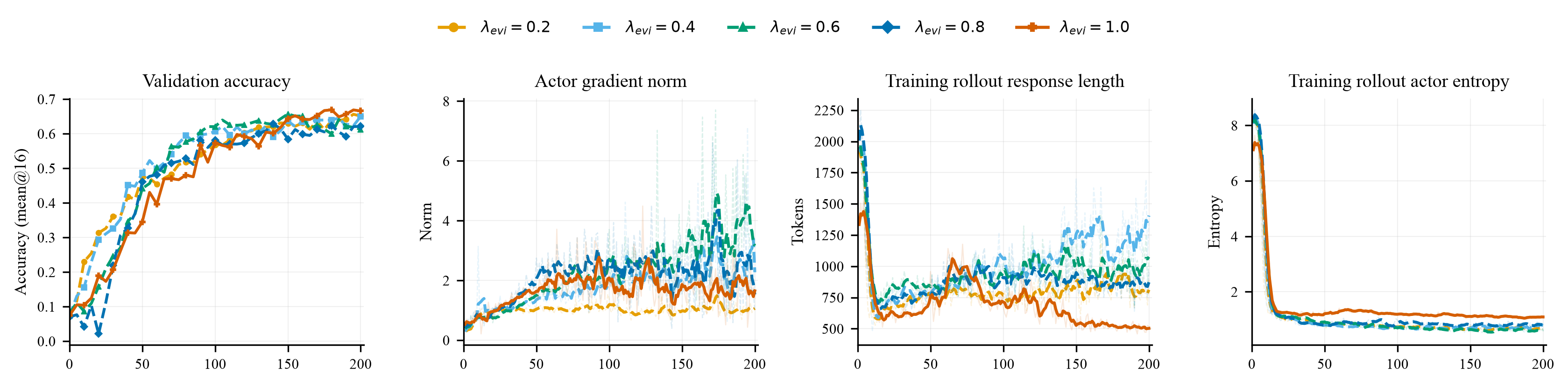
As shown in Figure 7, validation performance does not improve monotonically as $\lambda_{\mathrm{evi}}$ increases. The configuration $\lambda_{\mathrm{evi}}=1.0$ has the highest displayed endpoint accuracy and matches the default in Table 15. This single-task comparison supports that choice among the plotted settings, without establishing an optimal coefficient across backbones or tasks.

D.5 Probability Mass Retention under Top-K Truncation

To assess the vocabulary approximation in Appendix F.4, we examine the first 200 steps of five Llama-3.2-1B-Instruct (Meta, 2024) FEC runs, one per task. All use FKL, joint loss weighting and advantage modulation, all-trajectory evidence routing, and EMA decay 0.95. The evidence-loss and advantage-modulation coefficients both equal 1. These diagnostics concern the joint update configuration, not the single-path main-table runs.

Support construction and measurement.

The correction support $S$ combines the top 128 candidates from each of $q^{+}$ , $q^{-}$ , and $q^{0}$ with the sampled token and removes duplicates. Thus $K=128$ specifies candidates per branch, not the final support size. The reference channel uses a separate support $S_{\mathrm{ref}}$ formed from its own top 128 candidates and the sampled token. All selected probabilities retain the full softmax normalization, without renormalizing the selected coordinates or adding a tail bucket. For a distribution $q$ , retained mass on $S$ is $M=\sum_{v\in S}q(v)$ . Figure 8 reports the logged token means of $1-M$ . The positive Teacher, negative Teacher, and Actor share $S$ , whereas the reference mass uses $S_{\mathrm{ref}}$ .

Figure 8: Omitted probability mass over the first 200 training steps for five FEC-LW+AM runs on Llama-3.2-1B-Instruct (Meta, 2024). The underlying observations are step means over routed valid response tokens. Lower values indicate greater probability retention on the selected support. The first three panels use the shared evidence-correction support, and the reference panel uses its independent support. The logarithmic axes show centered five-step moving averages within contiguous valid segments, with segment endpoints preserved. Colors, line styles, and markers distinguish tasks. Gaps mark zero-token steps and are not interpolated. Each task has one run, so the curves do not provide uncertainty estimates across seeds.

Observed retention.

All numerical summaries use unsmoothed observations. Each logged mass averages over routed valid response tokens before acceptance weighting. We aggregate steps using their logged token counts, rather than averaging step means equally. In task order Biology, Chemistry, Materials, Physics, and Tool Use, the 200-step window contains 175, 195, 199, 199, and 200 valid observations per branch. The remaining steps have zero selected-token counts and contribute neither to the plot nor to the averages. Across the five tasks and four branches, token-weighted retained mass ranges from 95.92% to 99.32%, while the step-200 means range from 99.62% to 99.88%. The task-specific token-weighted mean correction-support sizes range from 148.26 to 171.33 coordinates. These measurements support $K=128$ as a compact support with high aggregate probability retention in the tested configuration. Retention is not uniformly high throughout training. The lowest valid step mean is 28.90% in the early Chemistry reference trace, and the plot retains these early low-coverage observations.

Exact truncated gradient.

To identify what truncation changes, consider one token with $p=\operatorname{softmax}(z)$ at unit temperature. Freeze $S$ , the signed direction $\Delta$ on its selected coordinates, and the nonnegative weight $w$ during differentiation. Define the zero-padded vector $\Delta_{S}(v)=\mathbf{1}[v\in S]\Delta(v)$ and the truncated loss $L_{S}=-w\sum_{v\in S}\Delta(v)\log p(v)$ . The softmax derivative $\partial\log p(v)/\partial z_{j}=\mathbf{1}[v=j]-p(j)$ gives

s_{S}=\sum_{v\in S}\Delta(v),\qquad-\nabla_{z}L_{S}=w\bigl(\Delta_{S}-s_{S}p\bigr).

(D.1)

The extra term $-ws_{S}p$ comes from the live full-vocabulary normalizer. It acts on selected and omitted logits, ensuring that the logit update sums to zero even when the selected direction does not. Since $\|p\|_{1}=1$ and $w\geq 0$ , its absolute size satisfies

\bigl\|-\nabla_{z}L_{S}-w\Delta_{S}\bigr\|_{1}=w|s_{S}|.

(D.2)

Thus the simple direction $w\Delta_{S}$ recovers the negative loss gradient when $s_{S}=0$ , including a full-vocabulary difference of normalized endpoints. A small-vocabulary finite-difference check verifies both identities for nonzero mass defect, zero mass defect, full support, and zero weight, with maximum coordinate error below $3.2\times 10^{-12}$ .

Appendix E Diagnostic Metrics

To interpret the controller traces in Figure 5, this appendix defines their token sets, averaging rules, and inference limits. The four diagnostics describe acceptance and the measured FEC residual during training. They are not validation or test metrics. Let $\mathcal{I}_{\mathrm{route}}$ denote the valid response-token positions included by the evidence-route diagnostic mask. The implementation first sums each statistic and its token count across microbatches and data-parallel workers and then divides. Every mean below is therefore a global token-weighted mean rather than a mean of per-batch means. For the displayed FEC runs, the FEC diagnostic set equals $\mathcal{I}_{\mathrm{route}}$ . The mean definitions below require a nonempty diagnostic set. They do not specify a logging convention for empty sets.

E.1 ZPD Effective Weight Coverage

To measure the breadth of acceptance, $\mathrm{WeightEffectiveCoverage}$ counts diagnostic tokens whose stopped weight exceeds a fixed monitoring threshold:

\mathrm{WeightEffectiveCoverage}=\frac{1}{\left|\mathcal{I}_{\mathrm{route}}\right|}\sum_{(i,t)\in\mathcal{I}_{\mathrm{route}}}\mathbf{1}\!\left[w_{i,t}>\tau_{\mathrm{eff}}\right],\qquad\tau_{\mathrm{eff}}=10^{-3}.

(E.1)

The denominator counts routed diagnostic tokens, not every token in the batch. Coverage therefore measures acceptance conditional on this set and does not measure how often the routing mask selects tokens. The threshold is used only for monitoring and does not enter the controller. This metric differs from the strict nonzero fraction $\mathbf{1}[w_{i,t}>0]$ , which would count arbitrarily small numerical weights as active.

E.2 Mean Signed Benefit and Fisher Cost

To distinguish favorable and conflicting directions before rejection, we retain signed alignment in the benefit diagnostic. Equation (7) applies a positive part to this value for controller use. To expose rejected as well as accepted directions, the logged benefit diagnostic retains the value before this positive-part operation:

b_{i,t}=\widehat{A}_{i}(e_{y_{i,t}}-p_{i,t})^{\top}u_{i,t},\qquad h_{i,t}=[b_{i,t}]_{+}.

(E.2)

The one-hot score direction compares the evidence move with the sampled token’s outcome signal. Only $h_{i,t}$ enters the default acceptance rule. The logged metric $\mathrm{BenefitMean}$ , shown in the second panel of Figure 5, is

\mathrm{BenefitMean}=\frac{1}{|\mathcal{I}_{\mathrm{route}}|}\sum_{(i,t)\in\mathcal{I}_{\mathrm{route}}}b_{i,t}.

(E.3)

It is a raw signed mean, not the mean of $h_{i,t}$ and not a conditional mean over positive-benefit tokens. A negative value means that the signed evidence directions oppose the local GRPO (Shao et al., 2024) score direction on average. The default controller assigns zero weight to each token with nonpositive benefit, but a negative mean does not imply that every token is rejected. It also does not measure the reward change after an optimizer step.

The logged metric $\mathrm{FisherCostMean}$ , shown in the third panel, is the mean nonnegative Fisher movement term from Equation (7):

\mathrm{FisherCostMean}=\frac{1}{|\mathcal{I}_{\mathrm{route}}|}\sum_{(i,t)\in\mathcal{I}_{\mathrm{route}}}c_{i,t},\qquad c_{i,t}=u_{i,t}^{\top}F(p_{i,t})u_{i,t}\geq 0.

(E.4)

This nonnegative statistic measures local distribution movement, not observed reward loss. It is the unscaled dynamic term in the controller denominator. The full movement penalty is $\alpha_{\mathrm{cost}}c_{i,t}+\epsilon_{\mathrm{cost}}$ , so the plotted quantity excludes both the scale and the positive floor.

E.3 FEC Residual Nuisance Fisher Covariance

To check the aggregate residual left by the projection, $\mathrm{FECResidualCov}$ averages the signed Fisher covariance between the retained FEC residual in Equation (11) and the measured nuisance direction in Equation (10):

\mathrm{FECResidualCov}=\frac{1}{\left|\mathcal{I}_{\mathrm{FEC}}\right|}\sum_{(i,t)\in\mathcal{I}_{\mathrm{FEC}}}\left\langle\Delta_{i,t}^{\mathrm{FEC}},\Delta_{i,t}^{\mathrm{nuis}}\right\rangle_{F(p_{i,t})}.

(E.5)

Here $\mathcal{I}_{\mathrm{FEC}}$ contains the valid response-token positions on which the FEC branches and projection diagnostics are available. Equation (C.15) gives the remaining ridge-dependent covariance for each token under the coefficient in Equation (10).

A small mean signed covariance does not establish token-wise orthogonality. Positive and negative residuals can cancel in the average, and small vector norms also produce small covariance without a small angle. Figure 5 therefore provides an aggregate numerical check of the projection rather than a bound on every residual. Neither the sign nor the magnitude establishes a causal contribution to task accuracy.

Appendix F Experimental Details

To document the comparisons in Section 4, this appendix collects the data splits, runtime, shared training settings, method-specific coefficients, and supplied prompt templates. Hardware-specific timing runs are reported separately in Appendix G.

F.1 Datasets and Data Processing

We use the five-task benchmark release associated with SRPO (Li et al., 2026) as a fixed data source. Biology, Chemistry, Materials Science, and Physics are the Level-3 reasoning subsets of SciKnowEval (Feng et al., 2024). Tool Use is derived from ToolAlpaca (Tang et al., 2023). Table 12 reports the complete train and test splits used by every compared method.

Table 12: Five-task data splits shared by the compared methods. Counts denote examples rather than sampled responses.

Task	Source	Train	Test	Total
Biology	SciKnowEval (Feng et al., 2024) Level 3	450	50	500
Chemistry	SciKnowEval (Feng et al., 2024) Level 3	1,890	210	2,100
Materials Science	SciKnowEval (Feng et al., 2024) Level 3	841	94	935
Physics	SciKnowEval (Feng et al., 2024) Level 3	720	80	800
Tool Use	ToolAlpaca (Tang et al., 2023)	4,046	68	4,114
Total	–	7,947	502	8,449

The fixed splits prevent data membership from changing across methods. Science prompts request one of four answer options, while Tool Use prompts provide the available tool specifications. The literal input scaffolds are given in Appendix F.5.

F.2 Models, Baselines, and Runtime

To separate model and runtime choices from method coefficients, we summarize the Actor initialization, hardware profile, and thinking-mode switches are summarized in Table 13. The three listed models were full-parameter fine-tuned. The shared benchmark profile uses eight GPUs per run. The two-GPU Llama cost study in Appendix G is a separate hardware setting and is not pooled with the eight-GPU timing comparison. The implementation is built on verl (Sheng et al., 2025), uses PyTorch FSDP2 (Feng et al., 2025) for distributed Actor training, and uses vLLM (Kwon et al., 2023) for batched rollout generation. We use AdamW (Loshchilov and Hutter, 2019) for optimization.

F.3 Shared Training Setup

To define the common sampling and optimization budget, Table 13 separates rollout settings from validation decoding. These settings describe matched benchmark runs, not the hardware-specific cost profiles. Table 15 then isolates the coefficients and support approximation used by VERPO.

Table 13: Common benchmark, runtime, and optimization settings used by matched experiments.

Parameter	Value
Actor initialization	Qwen3-4B (Yang et al., 2025), Qwen3-8B (Yang et al., 2025), Llama-3.2-1B-Instruct (Meta, 2024)
Hardware	8 $\times$ NVIDIA A800 GPUs per run
Actor / Teacher / validation thinking	False / False / False
Global prompt batch / rollouts per prompt	32 / 8
Mini-batch trajectories / update epochs	32 / 1
Maximum prompt / response length	2,048 / 8,192 tokens
Maximum reprompt / model length	10,240 / 18,944 tokens
Training decoding	temperature 1.0, top- $p$ 1.0, top- $k$ disabled
Validation decoding	16 rollouts, temperature 0.6, top- $p$ 0.95, top- $k$ disabled
Outcome clipping	upper radius $\epsilon_{\mathrm{high}}=0.28$
Optimizer	AdamW (Loshchilov and Hutter, 2019), weight decay 0.01, gradient clip 1.0
Schedule	constant after 10 warmup steps
Budget	200 optimizer steps

F.4 Method-Specific Hyperparameters

To distinguish algorithm settings from the shared budget, Table 14 lists the baseline configurations. Their Jensen-Shannon divergence (Lin, 1991) is the symmetric distillation divergence, distinct from the FKL and RKL decompositions used for VERPO. Table 15 separates VERPO’s reference and evidence coefficients from its controller parameters. Given the benefit and cost proxies, the acceptance fraction uses $\alpha_{\mathrm{cost}}$ and $\epsilon_{\mathrm{cost}}$ . The projection ridge instead changes the evidence direction before weighting.

Table 14: Baseline-specific loss and optimizer settings. Dashes preserve entries not specified for the corresponding baseline.

Outcome loss
Parameters	GRPO (Shao et al., 2024)	SDPO (Hübotter et al., 2026)	SRPO (Li et al., 2026)
Asymmetric upper clip $\epsilon_{\mathrm{high}}$	0.28	–	0.28
Rollout IS clip $\rho$	–	–	2.0
KL coefficient	0.0	–	0.0
Distillation loss
Top- $K$ distillation	–	100	100
Distillation divergence	–	Jensen-Shannon (Lin, 1991)	Jensen-Shannon (Lin, 1991)
EMA update rate	–	0.05	0.05
Rollout IS clip $\rho$	–	2.0	2.0
Dynamic weighting
Dynamic-weighting coefficient $\beta$	–	–	1
Training
Optimizer	AdamW (Loshchilov and Hutter, 2019)	AdamW (Loshchilov and Hutter, 2019)	AdamW (Loshchilov and Hutter, 2019)
Learning rate	$5\times 10^{-6}$	$1\times 10^{-5}$	$5\times 10^{-6}$
Warmup steps	10	10	10
Weight decay	0.01	0.01	0.01
Gradient clip norm	1.0	1.0	1.0

Table 15: VERPO-specific hyperparameters.

Parameter	Value
$\lambda_{\mathrm{ref}}$	0.1
$\lambda_{\mathrm{evi}}$	1.0
Direction construction	Fix (Hübotter et al., 2026), CTR (Pan et al., 2026), FEC
KL geometry	FKL, RKL
ZPD cost coefficient $\alpha_{\mathrm{cost}}$	0.0025
ZPD denominator floor $\epsilon_{\mathrm{cost}}$	$2.5\times 10^{-5}$
FEC ridge	$10^{-8}$
Teacher candidates per branch	Top- $K=128$
Vocabulary chunk size	4,096
EMA Teacher decay	0.95

To reduce vocabulary computation, the implementation forms a deduplicated union of the top- $K$ candidates from the Teacher branches used by each correction and adds the sampled token. FKL FEC uses the three branches $q^{+}$ , $q^{-}$ , and $q^{0}$ . The RKL correction additionally includes the Actor’s top- $K$ candidates. Thus $K=128$ specifies candidates per branch, not the size of the final union.

Selected log probabilities retain their full-vocabulary softmax normalization. The omitted tail is neither renormalized into the selected coordinates nor represented by an extra bucket. Evidence losses, Fisher moments, and projection statistics on this support are therefore approximations to the full-vocabulary quantities in Appendix C. In particular, a truncated FKL displacement need not sum to zero on the selected coordinates, so the exact full-vocabulary logit identities cannot be assumed unchanged after truncation. Support selection, Teacher values, and projection coefficients are stopped during Actor differentiation, while the Actor softmax normalizer remains live. Appendix D.5 gives the exact truncated logit gradient and measures probability retention for $K=128$ over 200 training steps.

The EMA decay of 0.95 weights the previous Teacher state in Equation (B.7), leaving an update rate of 0.05. This distinction avoids interpreting decay and update rate as the same parameter.

F.5 Prompt Templates

To make the task formatting explicit, the following listings preserve the supplied prompt text, including literal placeholders, punctuation, and response tags. The science system message constrains the final output to an option letter, while its user message supplies the question and options.

⬇

Given a question and four options, please select the right answer. Respond in the following format:

…

</reasoning>

…

</answer>

For the answer, only output the letter corresponding to the correct option (A, B, C, or D), and nothing else. Do not restate the answer text. For example, if the answer is ”A”, just output:

</answer>

⬇

[record-specific question and four answer options]

Please reason step by step.

The Tool Use messages restrict the Actor to the supplied tools and specify the action-call format. Record-specific API descriptions and schemas occupy the indicated placeholder rather than a shared fixed tool list.

⬇

You are a tool-use assistant. Solve each request by reasoning about the task and calling the provided tools when needed.

Use only the tools provided in the user message.

Follow the required response format exactly.

⬇

Your task is to answer the user’s question using available tools.

You have access to the following tools:

[record-specific tool names, descriptions, API documentation,

parameter schemas, and output schemas]

Use the following format:

Thought: you should always think about what to do

Action: the action to take, should be one of the tool names.

Action Input: the input to the action, must be in JSON format. All of the action input must be realistic and from the user.

Begin!

Question: [record-specific question]

The final listing shows the positive-evidence Teacher scaffold. It augments the task prompt with privileged context before replaying the sampled prefix as defined in Equation (B.6). This supplied scaffold does not specify the exact incorrect-evidence serialization for every contrastive branch.

⬇

[original task user prompt]

Correct solution:

[validated privileged context or selected sibling response]

Correctly solve the original question.

Appendix G Computational Analysis

To put the accuracy comparisons in computational context, this appendix reports logged step costs and the approximate compute-matched comparison discussed with Table 3. The Llama-3.2-1B measurements use two A800 GPUs, while the Qwen3-4B Chemistry measurements use eight. These hardware groups are evaluated separately.

G.1 Per-Step Cost

To distinguish total step cost from the recorded component timers, Tables 16 and 17 retain the generation, Teacher/evidence, and Actor-update columns alongside the logged total. Each entry averages its corresponding logged statistic over steps 10 to 200. The component values do not form an additive wall-clock decomposition. We preserve the reported timers without summing them to reconstruct the total or inferring an overlap schedule.

Table 16: Logged Llama-3.2-1B computation costs on two A800 GPUs over steps 10 to 200. Gen denotes generation. Peak alloc. denotes logged peak allocated memory. Component timers must not be added to reconstruct total step time.

Method	Hardware	Gen	Teacher/evidence	Actor update	Total step	Throughput	Peak alloc.
		s/step	s/step	s/step	s/step	tok/s/GPU	GB
Fixed (Hübotter et al., 2026)	2×A800	7.21	53.48	12.30	23.30	508.4	10.77
CTR (Pan et al., 2026)	2×A800	10.92	53.99	14.84	29.68	638.9	11.66
FEC	2×A800	15.53	54.20	15.58	35.20	1021.4	12.30

Table 17: Logged Qwen3-4B Chemistry computation costs on eight A800 GPUs over steps 10 to 200. N/A means that the corresponding Teacher/evidence timer was not available, not that the method performed no Teacher computation. The same nonadditive timing caveat as Table 16 applies.

Method	Hardware	Gen	Teacher/evidence	Actor update	Total step	Throughput	Peak alloc.
		s/step	s/step	s/step	s/step	tok/s/GPU	GB
GRPO (Shao et al., 2024)	8×A800	22.52	N/A	17.58	48.50	466.8	16.20
SDPO (Hübotter et al., 2026)	8×A800	3.32	N/A	28.84	40.80	278.8	35.07
SRPO (Li et al., 2026)	8×A800	5.98	N/A	27.51	42.20	309.2	23.07
VERPO	8×A800	31.09	176.34	42.14	82.41	281.5	18.81

In Table 16, Fixed (Hübotter et al., 2026) has a logged total of 23.30 seconds per step, compared with 29.68 for CTR (Pan et al., 2026) and 35.20 for FEC. This ranks the observed step costs but does not establish equal training quality. In particular, the Fixed-direction experiments exhibited reward hacking as reported with Table 4.

In Table 17, VERPO records 82.41 seconds per step compared with 48.50 for GRPO (Shao et al., 2024). Its reported peak allocation is 18.81 GB, compared with 16.20 GB for that baseline and 35.07 GB for SDPO (Hübotter et al., 2026). These are measurements from the listed profiles. Throughput alone does not rank end-to-end efficiency because generated token counts and response lengths differ. The recorded peak-allocation field also does not establish whether worker aggregation uses a maximum or another reduction.

G.2 Compute-Matched Performance

To compare quality at an approximately shared budget, we evaluate VERPO, GRPO (Shao et al., 2024), SDPO (Hübotter et al., 2026), and SRPO (Li et al., 2026) on the same Llama-3.2-1B backbone and $2\times$ A800 hardware in Table 18. For each run, we estimate the training compute based on the average wall-clock time per optimization step after the initial warm-up period. The budget for each task is defined by the compute required for the corresponding 200-step outcome-only baseline, and the nearest available five-step validation checkpoint is selected for the other methods.

Table 18: Approximate compute-matched Llama-3.2-1B results. Each method cell reports matched step / validation accuracy. The budget row gives the task-specific target in A800 GPU-hours. Accuracy averages 16 sampled responses per evaluation example, with higher values indicating better performance. Checkpoint matching is approximate.

Method	Biology	Chemistry	Materials	Physics	Tool Use	Average
Budget, GPU-h	10.91	11.53	10.61	9.97	10.08	10.62
VERPO	105 / 0.5100	105 / 0.5661	85 / 0.4570	85 / 0.4914	90 / 0.4885	94 / 0.5026
GRPO (Shao et al., 2024)	200 / 0.4988	200 / 0.5247	200 / 0.4348	200 / 0.4867	200 / 0.4504	200 / 0.4791
SDPO (Hübotter et al., 2026)	150 / 0.0862	150 / 0.0018	145 / 0.1117	125 / 0.3984	110 / 0.3107	136 / 0.1818
SRPO (Li et al., 2026)	145 / 0.3187	160 / 0.5649	130 / 0.3191	125 / 0.4313	160 / 0.4428	144 / 0.4154

VERPO has the highest reported accuracy in each of the five task columns. Its average of 0.5026 exceeds the 0.4791 from GRPO (Shao et al., 2024) by 0.0235, at an average of 94 rather than 200 optimizer steps. These results support a quality advantage under the estimated budgets on this backbone. They do not show lower per-step cost or exact equality of consumed GPU-hours. Averaged step times and five-step checkpoint spacing make the match approximate, and the table contains no uncertainty estimates across repeated runs.

Appendix H Case Study

To illustrate the weight allocation summarized in Appendix D.3, Figure 9 shows one matched pair of correct and incorrect rollouts for a Materials question. Both trajectories contain weighted reasoning tokens, so nonzero acceptance is not restricted to responses with a correct final answer. The displayed weights were computed offline with both trajectory classes eligible.

Darker text groups mark greater mean acceptance under the local benefit and cost proxies, not an estimated causal contribution to the answer. Uncolored groups fall below the figure’s coloring threshold, which does not establish that they are irrelevant to reasoning. This example illustrates nonuniform allocation within two responses rather than a general ordering of token importance.

VERPO: Verified Evidence Regularized Policy Optimization