AVSplat: Dense-View Feed-Forward 3D Gaussian Splatting with Assist-View Preconditioning
Abstract
Pose-free feed-forward 3D Gaussian Splatting enables novel view synthesis from uncalibrated multi-view images. Although more views should improve performance, existing methods often degrade with dense-view inputs because global aggregation spreads attention over many tokens, and naive voxel fusion averages many Gaussians into overly smooth representations. We present AVSplat, a framework that turns additional views into reliable signals for both aggregation and representation. Before global attention, each view performs a single lightweight interaction with a small set of Assist Views chosen for relevance and diversity, and the cached features provide a focused scene context that stabilizes correspondence. For representation, we use adaptive temperature-aware voxel fusion that sharpens attribution under high occupancy, guided by occupancy and point confidence. Crucially, AVSplat restores positive view scaling where performance remains stable or improves as more input views are added, instead of degrading in the dense-view regime. Ablations show that Assist View Preconditioning is primarily responsible for preventing dense-view degradation, while Occupancy-guided Voxel Fusion contributes most of the single-point image-quality gains.
Keywords:
3D Gaussian Splatting Novel View Synthesis Pose-Free Reconstruction Dense-View Reconstruction1 Introduction
Recent feed-forward 3D Gaussian Splatting (3DGS) [12, 22, 26, 6, 5] enables pose-free novel view synthesis from uncalibrated multi-view images. A single forward pass predicts camera intrinsics and extrinsics together with a compact set of Gaussian primitives for differentiable rasterization. These advances are based on geometric foundation models that infer structure directly from images. DUSt3R [15] and MASt3R [8] estimate dense point maps and pixel correspondences so downstream reconstruction can use point-level supervision without precomputed calibration. VGGT [14] estimates camera parameters, point maps, depth maps, and point tracks from one or many views and simplifies multi-view reasoning. Feed-forward 3DGS systems adopt such backbones and encode images with a geometry transformer before decoding features into Gaussian parameters and camera poses. This unifies geometric inference and radiance representation within a single pass.
Despite this progress, scaling from a few input views toward dense input views often yields a counterintuitive outcome in which reconstruction fidelity decreases as the number of input views increases [5, 16]. Two common design choices explain this behavior. The first lies in the global aggregation of the backbone [14] when the sequence length grows without known poses. In the absence of known poses, global aggregation relies on softmax attention to discover correspondences across many tokens. As the sequence length grows, the attention mass diffuses over many candidates, reducing the weight assigned to correct matches and weakening cross-view consistency [13]. The second lies in voxel fusion [5]. Per-pixel Gaussians are aggregated into a voxel grid to support efficient differentiable rasterization. When many Gaussians fall into the same voxel, a normalized average behaves as a low-pass filter. Strong contributors are diluted by many weak ones and high-frequency detail is lost. The issue becomes worse when the confidence of the contributor varies, but the fusion weights are not adaptive.
We propose AVSplat to improve global correspondence reasoning and voxel representation in the dense-view setting. We first propose an Assist View Preconditioning module. This module is designed to address a dense-view failure mode of prior pose-free pipelines, where the global attention becomes increasingly diffuse and cross-view matching becomes unstable as the number of input views grows. In this module, each current view performs a single lightweight interaction with a small Assist View set before any global attention. The Assist Views are both relevant to the current view and complementary to each other. Selection first finds strong neighbors by embedding similarity, then promotes diversity with a coverage-aware criterion, so that a small budget captures complementary observations and improves scene coverage. The features of Assist Views are cached for efficiency. The current view attends to these features and obtains conditioned tokens that carry the scene context before global aggregation. This focuses the correspondence search on plausible matches and reduces attention dispersion. A gated residual controls conditioning strength early in training and stabilizes optimization.
AVSplat also introduces Occupancy-guided Voxel Fusion, which adapts the fusion temperature to voxel occupancy and local consistency. High occupancy produces a sharper weight distribution, allowing reliable contributors to dominate the fused attributes. Under low occupancy, a smoother distribution retains information from multiple candidates and avoids brittle winner-take-all fusion. The temperature is constrained to a fixed range to stabilize optimization, while multi-view agreement and photometric residuals reduce the influence of outliers. This design helps preserve high-frequency structure in crowded voxels.
By converting additional views into a useful signal during both aggregation and representation, AVSplat preserves detail under high voxel occupancy and keeps correspondence search focused at long sequence length. In pose-free settings, it consistently improves overall performance with more input views under comparable compute and memory. Ablations confirm that Assist View Preconditioning and Occupancy-guided Voxel Fusion are both necessary for consistent gains. The analysis explains why prior feed-forward pipelines degrade when inputs become dense and shows that modeling attention sparsity and voxel attribution together leads to scalable and high-fidelity 3D Gaussian Splatting.
Our main contributions are:
- •
We present AVSplat, a pose-free feed-forward framework that maintains positive view scaling in dense multi-view settings through improvements in global aggregation and voxel representation.
- •
We introduce Assist View Preconditioning, a lightweight per-view conditioning step that restores positive view scaling by preventing attention dilution and stabilizing cross-view matching at long sequence lengths.
- •
We propose Occupancy-guided Voxel Fusion, where the sampling distribution varies with the voxel occupancy and local consistency so that high-frequency detail is preserved.
- •
We conduct extensive experiments in pose-free settings, showing that AVSplat maintains or improves performance as the number of input views increases.
2 Related Work
2.1 Geometry foundation models
Recent geometry foundation models predict dense point maps and correspondences directly from few views. DUSt3R [15] recovers accurate point maps without calibration, providing strong priors for reconstruction and tracking. MASt3-R [8] grounds the matching in 3D, producing robust, coarse-to-fine correspondences under wide baselines. MUSt3R [2] extends to multi-view sequences and enables high-frame-rate inference for offline or online reconstruction. VGGT [14] advances the foundation model line by inferring camera parameters, depth, point maps, and point tracks in a single pass from one view to many views. The model alternates frame-wise and global aggregation and therefore reasons jointly over all frames. The approach improves the accuracy of feed-forward reconstruction and reduces reliance on multi-stage optimization. Analyses of global attention in VGGT and in related transformers reveal a dominant runtime cost that grows quadratically with sequence length and a sparse pattern in which a small set of patch interactions carries most probability mass. Replacing dense global attention with block sparse kernels preserves accuracy while accelerating inference on long sequences.
2.2 Feed-forward 3D Gaussian Splatting
Feed-forward 3DGS predicts scene-specific Gaussians and renders novel views without per-scene optimization. PixelSplat [3] learns from image pairs with a 3D probability field for stable training and real-time rendering. MVSplat [4] uses plane-sweep cost volumes to extract clean Gaussians from sparse multi-view inputs. DepthSplat [19] couples splatting with monocular depth, yielding mutual gains. MuSASplat [21] improves pose-free sparse-view 3DGS through lightweight multi-scale adaptation and efficient cross-view feature fusion, while ZPressor [16] compresses multi-view inputs into a compact latent state, enabling feed-forward 3DGS models to scale to over 100 input views.
Pose-free and COLMAP-free pipelines operate on uncalibrated inputs. Splatt-3R [12] transfers MASt3R priors to stereo; NoPoSplat [22] anchors Gaussians in a canonical camera space for real-time inference; SelfSplat [6] removes external 3D priors via self-supervised depth and pose. FLARE [26] features a cascaded learning paradigm with camera pose serving as the critical bridge, achieving accurate camera pose estimation and high-quality 3D rendering. PCR-GS [18] tackles COLMAP-free 3DGS from a per-scene optimization perspective through pose co-regularization. In contrast, AVSplat follows the one-pass feed-forward setting and focuses on dense-view scaling.
Recent methods adopt geometry transformers: AnySplat [5] encodes uncalibrated collections with a VGGT-style aggregator and predicts Gaussians and poses with voxel-level grouping. Scaling to dense inputs exposes two issues—diluted global attention and high-occupancy voxel fusion that smooths high-frequency details—which we address by strengthening correspondence before global aggregation and refining fusion in crowded voxels.
Complementary 3DGS advances improve Gaussian representation, detail pre-servation, and controllable appearance. SOGS [23] introduces second-order anchors to improve anchor-based 3DGS with compact anchor features and reduced model size. FreGS [24] uses progressive frequency regularization to guide Gaussian densification from low to high frequencies and alleviate over-reconstruction. StyleGaussian [11] extends Gaussian splatting to instant 3D style transfer through efficient feature rendering and a KNN-based 3D CNN decoder. These works are orthogonal to AVSplat, which targets dense-view aggregation and voxel attribution in pose-free feed-forward reconstruction.
3 Method
This section first recalls the principles of 3D Gaussian Splatting [7] and the transformer-style multi-view geometry encoder (VGGT [14]) that we build upon. We then present the overall pipeline of our method. The pipeline extends the previous feed-forward Gaussian predictor [5] with two new components. The first component performs assist view preconditioning so that every input view receives compact scene context before global aggregation, with the primary goal of preventing dense-view degradation caused by attention dispersion. The second component performs occupancy-guided temperature fusion so that voxel-level attributes remain sharp under dense inputs.

3.1 Preliminaries
3D Gaussian Splatting
In 3D Gaussian Splatting (3DGS) [7], a scene is represented by a finite set of anisotropic Gaussians
| (1) |
Here is the mean, is a positive definite covariance, is the radiance and is the opacity. For a calibrated camera with projection and view direction , each Gaussian projects to the image plane as
| (2) |
where is the Jacobian of at . Let denote the induced 2D Gaussian kernel at pixel . Rendering proceeds in front-to-back order with color
| (3) |
and transmittance
| (4) |
Classical methods optimize per scene from multi-view supervision. Feed-forward 3DGS removes per-scene optimization. A network takes images and directly predicts together with camera intrinsics and extrinsics so that the rendering above supplies differentiable supervision in a single forward pass. The main challenges become multi-view feature aggregation and redundancy control in the predicted Gaussians.
Transformer style multi-view geometry encoder
In VGGT [14], a geom-etry-aware encoder receives a sequence of images and produces tokens that carry appearance and 3D structure. For each view the encoder yields patch tokens
| (5) |
Tokens are processed by alternating view-specific aggregation and global aggregation. The global stage operates on the concatenated set
| (6) |
This allows information to flow across views when poses are unknown. Special tokens can be attached to support the prediction of camera parameters, depth, and point tracks. Global aggregation has quadratic complexity in the number of tokens, and its attention maps tend to become increasingly diffuse as sequence length grows. Our method addresses this weakness.
3.2 AVSplat pipeline
Given uncalibrated images, the encoder produces view tokens. A scene-level aggregation consumes all tokens and produces latents for camera estimation and Gaussian prediction. From these latents we decode intrinsics, extrinsics, Gaussian centers, scales, orientations, colors, and opacities. The resulting Gaussians are voxelized and rendered. An overview of our pipeline is shown in Figure 1.
Our pipeline introduces two new designs. Before tokens enter global aggregation, we insert an assist view preconditioning module so that each view collects context from a compact set of assisting views. After Gaussian prediction, we replace uniform voxel fusion [5] with an occupancy-guided temperature fusion module that modulates fusion weights according to voxel occupancy and reliability. We refer to these modules as Assist View Preconditioning and Occupancy-guided Voxel Fusion.
3.3 Assist View Preconditioning
Global aggregation is expected to resolve correspondences across many views. When the number of views increases, tokens from unrelated views inflate the attention pool and the distribution becomes diffuse [13]. Tokens from geometrically compatible views receive less probability mass and long-range constraints fail to strengthen the global match. Each view should first collect context from a compact and diverse set of assisting views and should enter global aggregation with this context.
Coverage driven assist selection
For view with tokens we form a view descriptor by average pooling
| (7) |
We compute cosine similarity between views
| (8) |
A candidate pool is formed by the nearest neighbors of in descriptor space
| (9) |
To measure how well a candidate view supports the tokens of , we define a token-level support score. Let . Using a lightweight projection , the support from view to token of is
| (10) |
We then define a coverage objective over an assist set of size
| (11) | ||||
where is a view reliability term derived from token variance, the first term rewards token coverage, the second term prefers reliable helpers, and the third term discourages redundant views. Because the first term is monotone and submodular, greedy selection provides a near-optimal solution at low computational cost. Starting from , we update
| (12) |
until , where . In practice we evaluate on a stratified subset of tokens, cache per-view projections, and use random tie-breaking to improve generalization.
Lightweight conditioning
Given the selected assist set , we apply a single cross-view interaction to inject context. With linear maps absorbed into keys, queries, and values, the conditioned tokens are
| (13) |
where and are formed by concatenating tokens from the assist set and is obtained from . We combine original and conditioned tokens through a gated residual
| (14) |
where denotes the current training step and increases from near zero to one. The global aggregation then consumes .
This selection strategy favors views that cover different regions of the reference view and that agree with its content, while avoiding near duplicates. The single conditioning step moves the burden of discovery from the global module to the selection stage, so the subsequent aggregation focuses on long-range alignment rather than search. The resulting view-conditioned tokens are then fed into the same global aggregation and decoding heads as in the baseline.
3.4 Occupancy-guided Voxel Fusion
After obtaining all Gaussians, we project them onto a voxel grid so that Gaussians falling into the same or nearby voxels can be fused, reducing redundancy. Simple averaging within a voxel attenuates high-frequency appearance and smoo-ths fine-scale geometry, because numerous weak contributors dilute a few strong ones. The effect increases with occupancy and leads to over-smoothed reconstructions.
For voxel we define the candidate set and the occupancy , where is the index set of candidates that are assigned to voxel by the voxelization step. Each candidate provides a feature vector , a 3D point and a confidence . We define a temperature
| (15) |
with base temperature , exponent and bounds . The reliability factor depends on geometric consistency. We compute a variance
| (16) |
with mean and set
| (17) |
Here measures the dispersion of 3D points within the voxel. Voxels with small variance are more geometrically consistent and therefore assigned a larger reliability factor . We then form logits for and compute softmax weights
| (18) |
To reduce the influence of outliers, we sort candidates in descending order of and retain the shortest prefix whose cumulative weight reaches a target mass. The fused voxel feature and position are
| (19) |
High occupancy reduces the temperature and sharpens the distribution so that candidates with high confidence or strong geometric agreement dominate. Low occupancy yields a higher temperature so that the fusion remains inclusive. The procedure preserves detail in well-observed regions and remains robust where support is limited. All steps are differentiable and trained jointly with the rest of the network.
Our method changes the order of information integration and the way voxel attribution is formed. Previous methods bring all tokens into a single pool and rely on a global module to discover relations. Assist view preconditioning makes each view context-aware before that stage. Standard fusion treats all candidates inside a voxel as equal competitors. Occupancy-guided Voxel Fusion makes the voxel sensitive to both how many candidates it receives and how consistent they are. These changes address the main causes of saturation in dense-view feed-forward 3DGS and restore the behavior that more views improve reconstruction quality.
4 Experiments
4.1 Experimental setup
| Sparse inputs | |||||||||
| 3 | 6 | 16 | |||||||
| Method | PSNR | SSIM | LPIPS | PSNR | SSIM | LPIPS | PSNR | SSIM | LPIPS |
| Mip-NeRF 360 [1] | |||||||||
| NoPoSplat [22] | 16.36 | 0.430 | 0.453 | 15.92 | 0.416 | 0.541 | 15.47 | 0.361 | 0.606 |
| Flare [26] | 13.52 | 0.350 | 0.601 | 15.35 | 0.407 | 0.573 | 13.21 | 0.348 | 0.695 |
| AnySplat [5] | 17.29 | 0.429 | 0.433 | 17.51 | 0.446 | 0.412 | 17.81 | 0.448 | 0.382 |
| AVSplat | 17.33 | 0.451 | 0.354 | 17.99 | 0.467 | 0.352 | 18.13 | 0.428 | 0.390 |
| VR-NeRF [20] | |||||||||
| NoPoSplat [22] | 18.37 | 0.707 | 0.437 | 17.57 | 0.704 | 0.466 | 17.66 | 0.720 | 0.472 |
| Flare [26] | 18.58 | 0.717 | 0.470 | 18.26 | 0.717 | 0.477 | 17.02 | 0.709 | 0.510 |
| AnySplat [5] | 20.41 | 0.733 | 0.389 | 21.07 | 0.729 | 0.436 | 21.12 | 0.714 | 0.354 |
| AVSplat | 20.24 | 0.764 | 0.403 | 20.91 | 0.736 | 0.418 | 21.17 | 0.724 | 0.391 |
| DL3DV [9] | |||||||||
| AnySplat [5] | 15.04 | 0.387 | 0.612 | 15.74 | 0.420 | 0.492 | 17.43 | 0.542 | 0.419 |
| AVSplat | 14.41 | 0.341 | 0.598 | 15.62 | 0.424 | 0.492 | 17.80 | 0.565 | 0.344 |
| Dense inputs | |||||||||
| 32 | 48 | 64 | |||||||
| Mip-NeRF 360 [1] | |||||||||
| NoPoSplat [22] | OOM | OOM | OOM | ||||||
| Flare [26] | OOM | OOM | OOM | ||||||
| AnySplat [5] | 18.22 | 0.445 | 0.369 | 19.40 | 0.476 | 0.366 | 19.23 | 0.500 | 0.365 |
| AVSplat | 18.71 | 0.483 | 0.365 | 19.30 | 0.482 | 0.368 | 20.11 | 0.528 | 0.366 |
| VR-NeRF [20] | |||||||||
| NoPoSplat [22] | OOM | OOM | OOM | ||||||
| Flare [26] | OOM | OOM | OOM | ||||||
| AnySplat [5] | 21.11 | 0.711 | 0.380 | 21.60 | 0.745 | 0.338 | 21.26 | 0.719 | 0.350 |
| AVSplat | 21.42 | 0.720 | 0.365 | 21.62 | 0.734 | 0.317 | 21.7 | 0.723 | 0.363 |
| DL3DV [9] | |||||||||
| AnySplat [5] | 21.05 | 0.680 | 0.284 | 21.04 | 0.678 | 0.281 | 21.14 | 0.684 | 0.282 |
| AVSplat | 21.54 | 0.710 | 0.266 | 21.60 | 0.713 | 0.265 | 21.67 | 0.717 | 0.265 |


| Variant | PSNR | SSIM | LPIPS |
|---|---|---|---|
| Baseline | 21.14 | 0.684 | 0.282 |
| + Fusion only | 21.57 | 0.692 | 0.272 |
| + Assist + Fusion | 21.67 | 0.717 | 0.265 |
| Attention diagnostics | ACID overlap stress test | ||||
|---|---|---|---|---|---|
| Method | Entropy | GeoMass | Method | 48 views | 72 views |
| AnySplat | 0.693 | 0.286 | AnySplat | 23.12 | 22.45 |
| AVSplat | 0.642 | 0.374 | AVSplat | 23.15 | 23.24 |
Datasets
Our model is trained on the DL3DV dataset [9], which provides over 10k training scenes. Novel view synthesis quality is evaluated on Mip-NeRF 360 [1], VR-NeRF [20], and the DL3DV [9] test split. The DL3DV test split contains 140 scenes. For Mip-NeRF 360 and VR-NeRF we follow the settings used in prior work [5]. The sparse view setting uses 3, 6, and 16 input views per scene, and 2 target views per scene. The dense-view setting uses 32, 48, and 64 input views per scene, and 4, 6, and 8 target views, respectively. For VR-NeRF we use four indoor scenes that cover both compact and spacious layouts: apartment, kitchen, raf-furnishedroom, and workshop. For Mip-NeRF 360 we use four scenes with diverse viewpoints and lighting: bonsai, counter, kitchen, and room. These eight scenes span different room types, camera densities, and appearance patterns and are used for both sparse and dense-view evaluation. For each of the 140 DL3DV test scenes we first sample 75 candidate views, fix three random views as target views, and then randomly choose context views from the remaining views according to the desired input count.
Metrics and baselines.
We report PSNR, SSIM [17], and LPIPS [25]. SSIM is computed with a Gaussian window in linear color space. LPIPS uses the VGG backbone with official weights. Scores are first averaged over target views within each scene and then averaged over scenes. We compare with AnySplat [5] in the dense-view setting. The sparse view comparison includes NoPoSplat [22], FLARE [26], and AnySplat. Since evaluation on Mip-NeRF 360 and VR-NeRF is performed in a zero-shot setting, we retrain AnySplat on DL3DV using the public implementation and recommended configuration so that all methods share the same training data when comparing generalization performance.
4.2 Implementation details
Backbone and tokens
The backbone is a transformer-style multi-view geometry encoder derived from VGGT [14]. Images are resized to a shorter side of 518 with preserved aspect ratio. The encoder uses a patch size of 14, an embedding dimension of 1024, and 24 layers with 16 attention heads. Each view yields a grid of patch tokens and a small set of special tokens. A global aggregation stage consumes tokens from all views.
Training schedule
We train the model for 40,000 steps using AdamW with a learning rate of and a weight decay of . We use a cosine learning-rate schedule with 2,000 warm-up steps. Total steps are 40000. Mixed precision and activation checkpointing are enabled. Gradient norm is clipped at 1. During training, the number of input images per scene is a random integer in . Our model is trained with a batch size of 1 on a single NVIDIA A100 GPU with 80 GB memory.
Assist View Preconditioning
Each view selects 4 assisting views. We apply lightweight jittering with a probability of 0.05. The gating factor starts near 0 during a 2,000-step warm-up period and then increases linearly for 8000 steps until it reaches 1. We stop gradients through the assist branch for the first 1,500 steps. In the sparse-view setting, the number of available views is too small to form a meaningful assist set. Therefore, Assist-View Preconditioning is disabled in the sparse-view setting.
Occupancy-guided Voxel Fusion
Voxel fusion uses a temperature that varies with occupancy and reliability. The base temperature is 0.7. The occupancy exponent is 0.5. The reference count is 8. The temperature is clipped to . The geometric-variance term is assigned a weight of 2.0. We use a top-mass threshold of 0.8 to truncate low-weight candidates.
4.3 Results and analysis
Main results across sparse and dense inputs
Table 1 reports results for sparse inputs with 3, 6, and 16 views and dense inputs with 32, 48, and 64 views. AVSplat remains competitive across all three datasets and shows its clearest gains on DL3DV. In the sparse setting, AVP is disabled because too few views are available to form a meaningful assist set. Under dense inputs, AVSplat exhibits more stable improvements as the view count increases, which is the setting targeted by AVP and occupancy-guided fusion.
Figure 2 provides a qualitative comparison between AVSplat and AnySplat [5] under dense-view inputs. Since the artifacts we target primarily arise in the dense-view setting, we only show qualitative comparisons for dense-view inputs here. Consistent with the quantitative trends, regions highlighted by red boxes show that AVSplat recovers sharper surface details with fewer artifacts and less oversmoothing-induced blur. The rightmost column further indicates that AVSplat produces more accurate global matching, leading to better large-scale structural consistency in the reconstructed scenes.
Dense-view scaling and overlap stress test.
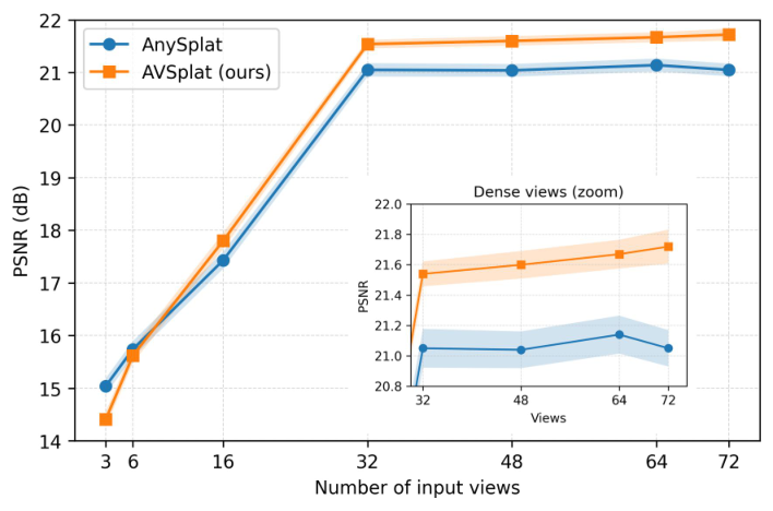
Under the fixed-target DL3DV protocol, AVSplat improves over AnySplat by 0.49, 0.56, and 0.53 dB at 32, 48, and 64 input views, respectively. More importantly, its PSNR continues to increase from 21.54 to 21.67 dB over this range, whereas the closest baseline largely saturates.
The difference becomes more pronounced for highly overlapping inputs. As shown in Table 3, on ACID [10], AnySplat decreases from 23.12 dB at 48 views to 22.45 dB at 72 views, whereas AVSplat increases from 23.15 to 23.24 dB, producing a 0.79 dB advantage at 72 views. The practical benefit is therefore not that every additional view produces a large single-step gain, but that redundant dense views no longer become harmful.
Attention analysis
We visualize the activations of the global aggregation stage in Figure 3 to better understand how assist-view preconditioning affects cross-view matching. For a fixed pair of input frames, we extract the post-softmax attention matrix from layer 15 of the full global-aggregation sequence. We remove special tokens and self-frame blocks, and then retain the cross-frame block corresponding to the selected pair. Given these tokens, we compute the attention matrix as , which yields a map where denotes the number of patch tokens per frame. The baseline exhibits diffuse attention mass when the number of views is large, indicating that global matching is poorly focused. In contrast, AVSplat produces attention patterns that are more sharply concentrated on geometrically plausible correspondences after preconditioning, demonstrating that our design effectively improves global matching.
4.4 Ablation studies
We ablate the Assist-View Preconditioning and Occupancy-guided Voxel Fusion modules in the 64-view setting on DL3DV [9]. Removing preconditioning reduces attention focus in the global aggregation stage and leads to lower PSNR and SSIM at long sequence lengths. Removing occupancy guidance causes excessive smoothing in high-occupancy regions, producing blur in the rendered images and suppressing fine surface details, which in turn degrades overall performance. As shown in Table 2, both components are effective. Occupancy-guided Voxel Fusion contributes most of the single-point image-quality improvement at 64 views, while Assist-View Preconditioning mainly targets the dense-view scaling failure mode by stabilizing global matching as the input count grows (see Figures 3 and 4).
Performance vs. Number of input views
Figure 4 further analyzes how performance scales with the number of input views. We plot PSNR for AVSplat and AnySplat using 3, 6, 16, 32, 48, 64, and 72 input views, with shaded bands indicating the standard deviation across multiple trials. Across the full range, both methods benefit substantially from moving from sparse to dense inputs. Beyond 32 views, however, their scaling behavior diverges. AnySplat begins to oscillate and slightly degrades at high view counts, whereas AVSplat continues to improve. The absolute gap at a fixed view count can be modest, but the scaling behavior differs consistently, which is the primary effect we target with Assist-View Preconditioning. This shows that AVSplat can consistently exploit additional views in dense settings, and complements the quantitative trends observed in Table 1.
Quantitative attention diagnostics.
To quantify the effect of AVP beyond the qualitative heatmaps in Fig. 3, we extract the post-softmax attention matrix from layer 15 of the full global-aggregation sequence. We exclude self-frame blocks and special tokens and average the results over four fixed view pairs. For cross-view attention , normalized entropy is the per-query entropy divided by the logarithm of the number of valid key patches. GeoMass@1patch is defined as where contains key patches within a one-patch-width epipolar band computed from ground-truth evaluation poses. As shown in Table 3, AVSplat reduces normalized entropy from 0.693 to 0.642 and increases GeoMass@1patch from 0.286 to 0.374, corresponding to an absolute gain of 8.8 points and a relative gain of 30.8%. The mass of a random band is approximately 0.10, so the concentration on geometrically compatible regions increases from approximately to the random baseline.
5 Conclusion
This work addresses dense-view degradation in pose-free feed-forward 3D Gaussian Splatting. Assist-View Preconditioning conditions each view before global aggregation, while Occupancy-guided Voxel Fusion adapts voxel weights to occupancy and reliability. Experiments on Mip-NeRF 360,VR-NeRF, and DL3DV show more stable performance as the number of input views increases, and the attention analysis and ablations support the contributions of the two modules. Together, these changes improve dense-view pose-free reconstruction without per-scene optimization.
Acknowledgements
This work was supported in part by the Ministry of Education, Singapore, under the Tier-2 project scheme (Project No. MOE-T2EP20123-0003), and in part by the U.S. National Science Foundation under Grant No. CRCNS-2309041.
References
- [1] (2022) Mip-nerf 360: unbounded anti-aliased neural radiance fields. In Proceedings of the IEEE/CVF conference on computer vision and pattern recognition, pp. 5470–5479. Cited by: §4.1, Table 1, Table 1, Table 1, Table 1.
- [2] (2025) Must3r: multi-view network for stereo 3d reconstruction. In Proceedings of the Computer Vision and Pattern Recognition Conference, pp. 1050–1060. Cited by: §2.1.
- [3] (2024) Pixelsplat: 3d gaussian splats from image pairs for scalable generalizable 3d reconstruction. In Proceedings of the IEEE/CVF conference on computer vision and pattern recognition, pp. 19457–19467. Cited by: §2.2.
- [4] (2024) Mvsplat: efficient 3d gaussian splatting from sparse multi-view images. In European Conference on Computer Vision, pp. 370–386. Cited by: §2.2.
- [5] (2025) AnySplat: feed-forward 3d gaussian splatting from unconstrained views. arXiv preprint arXiv:2505.23716. Cited by: §1, §1, §2.2, §3.2, §3, Figure 2, Figure 2, Figure 4, Figure 4, §4.1, §4.1, §4.3, Table 1, Table 1, Table 1, Table 1, Table 1, Table 1.
- [6] (2025) SelfSplat: pose-free and 3d prior-free generalizable 3d gaussian splatting. In Proceedings of the Computer Vision and Pattern Recognition Conference, pp. 22012–22022. Cited by: §1, §2.2.
- [7] (2023) 3D gaussian splatting for real-time radiance field rendering.. ACM Trans. Graph. 42 (4), pp. 139–1. Cited by: §3.1, §3.
- [8] (2024) Grounding image matching in 3d with mast3r. In European Conference on Computer Vision, pp. 71–91. Cited by: §1, §2.1.
- [9] (2024) Dl3dv-10k: a large-scale scene dataset for deep learning-based 3d vision. In Proceedings of the IEEE/CVF Conference on Computer Vision and Pattern Recognition, pp. 22160–22169. Cited by: §4.1, §4.4, Table 1, Table 1, Table 1, Table 1, Table 2, Table 2.
- [10] (2021) Infinite nature: perpetual view generation of natural scenes from a single image. In Proceedings of the IEEE/CVF International Conference on Computer Vision, pp. 14458–14467. Cited by: §4.3.
- [11] (2024) Stylegaussian: instant 3d style transfer with gaussian splatting. In SIGGRAPH Asia 2024 Technical Communications, pp. 1–4. Cited by: §2.2.
- [12] (2024) Splatt3r: zero-shot gaussian splatting from uncalibrated image pairs. arXiv preprint arXiv:2408.13912. Cited by: §1, §2.2.
- [13] (2025) Faster vggt with block-sparse global attention. arXiv preprint arXiv:2509.07120. Cited by: §1, §3.3.
- [14] (2025) Vggt: visual geometry grounded transformer. In Proceedings of the Computer Vision and Pattern Recognition Conference, pp. 5294–5306. Cited by: §1, §1, §2.1, §3.1, §3, §4.2.
- [15] (2024) Dust3r: geometric 3d vision made easy. In Proceedings of the IEEE/CVF Conference on Computer Vision and Pattern Recognition, pp. 20697–20709. Cited by: §1, §2.1.
- [16] (2025) ZPressor: bottleneck-aware compression for scalable feed-forward 3dgs. arXiv preprint arXiv:2505.23734. Cited by: §1, §2.2.
- [17] (2004) Image quality assessment: from error visibility to structural similarity. IEEE transactions on image processing 13 (4), pp. 600–612. Cited by: §4.1, Table 1, Table 1.
- [18] (2025) PCR-gs: colmap-free 3d gaussian splatting via pose co-regularizations. In Proceedings of the IEEE/CVF International Conference on Computer Vision, pp. 26499–26508. Cited by: §2.2.
- [19] (2025) Depthsplat: connecting gaussian splatting and depth. In Proceedings of the Computer Vision and Pattern Recognition Conference, pp. 16453–16463. Cited by: §2.2.
- [20] (2023) VR-nerf: high-fidelity virtualized walkable spaces. In SIGGRAPH Asia 2023 Conference Papers, pp. 1–12. Cited by: §4.1, Table 1, Table 1, Table 1, Table 1.
- [21] (2026) MuSASplat: efficient sparse-view 3d gaussian splats via lightweight multi-scale adaptation. In Proceedings of the AAAI Conference on Artificial Intelligence, Vol. 40, pp. 11343–11351. Cited by: §2.2.
- [22] (2024) No pose, no problem: surprisingly simple 3d gaussian splats from sparse unposed images. arXiv preprint arXiv:2410.24207. Cited by: §1, §2.2, §4.1, Table 1, Table 1, Table 1, Table 1.
- [23] (2025) Sogs: second-order anchor for advanced 3d gaussian splatting. In Proceedings of the IEEE/CVF Conference on Computer Vision and Pattern Recognition, pp. 11167–11176. Cited by: §2.2.
- [24] (2024) Fregs: 3d gaussian splatting with progressive frequency regularization. In Proceedings of the IEEE/CVF Conference on Computer Vision and Pattern Recognition, pp. 21424–21433. Cited by: §2.2.
- [25] (2018) The unreasonable effectiveness of deep features as a perceptual metric. In Proceedings of the IEEE conference on computer vision and pattern recognition, pp. 586–595. Cited by: §4.1, Table 1, Table 1.
- [26] (2025) Flare: feed-forward geometry, appearance and camera estimation from uncalibrated sparse views. In Proceedings of the Computer Vision and Pattern Recognition Conference, pp. 21936–21947. Cited by: §1, §2.2, §4.1, Table 1, Table 1, Table 1, Table 1.
Supplementary Material
6 Additional Algorithmic Details
6.1 Assist-View Preconditioning (Sec. 3.3)
Before any global aggregation, we precondition the per-view patch tokens by letting each view attend to a small set of assist views. For a batch element, let denote the patch-token grid of view , with spatial tokens and embedding dimension . We first compute a descriptor for each view and a subsampled token set for coverage, obtained by regularly sampling tokens and normalizing them.
For each target view , we construct a candidate pool using nearest neighbors in descriptor space (cosine similarity). Among these candidates, we greedily pick assist views by maximizing a score that combines: (i) similarity of the candidate descriptor to the target descriptor, (ii) diversity with respect to already selected assist views in descriptor space, (iii) token-level coverage gain on , and (iv) a reliability score derived from within-view token variance. The greedy procedure runs on detached tokens and descriptors, so the selection is treated as a non-differentiable side computation.
Given the selected assist set , we perform one multi-head attention (MHA) per view with queries from the current view and keys/values from the assist views. The resulting context is added back as a gated residual:
and afterwards, where is the global training step, is a piecewise-linear gate that ramps from to , and is the MHA output. In our implementation we use , a warm-up of steps, a ramp of steps, and stop gradients from the assist-view branch for the first steps.
6.2 Occupancy-Guided Voxel Fusion (Sec. 3.4)
We fuse per-pixel 3D points and features into a sparse set of voxels using an occupancy- and reliability-aware temperature. Let and denote the 3D position and feature of sample (coming from all views and pixels), and let be an optional confidence. We discretize the positions into voxels of size via and group samples by voxel index. For each voxel , we compute:
- •
occupancy ,
- •
mean position and normalized variance ,
- •
geometric consistency ,
- •
mean confidence (after mapping to probability if needed),
- •
reliability as a weighted combination of and .
The voxel temperature is then
so dense, reliable voxels use a smaller temperature and produce sharper weights, while sparse or unreliable voxels use a larger temperature to avoid overconfident fusion. For each voxel we apply a per-voxel softmax (or sparsemax) with logits scaled by , optionally trim a prefix of weights until a cumulative mass threshold (e.g., ), and renormalize. The fused voxel position and feature are the weighted averages under these final weights.
7 More qualitative results
We provide more qualitative results in the format of videos. Please refer to the video in the supplementary materials.