Dynamic Windowing in Transformers via Regime Incorporation for Financial Time Series
Abstract
Financial time series exhibit non-stationary behavior, where the strength and extent of temporal dependencies change across market regimes. Trending low-volatility phases typically require long-range contextual information, whereas mean-reverting high-volatility periods rely more heavily on short-term dynamics. Standard Transformer architectures, with fixed attention windows and static positional encodings, are therefore unable to adapt to such variations. In this work, we propose a regime-aware dynamic windowing framework that incorporates market regime information directly into the Transformer. We construct four generic regime signals from the price series—volatility ratio, trend strength, local predictability ratio (LPR), and rolling autocorrelation—and embed them into the model through two mechanisms: (i) regime-augmented inputs to standered architecture, and (ii) a modified attention layer that modulates the attention weights using regime embeddings. Experiments on 5 S&P 500 stocks show consistent improvements across five evaluation metrics, demonstrating that regime-aware dynamic windowing enhances both explanibility and predictive performance in financial forecasting tasks.
I Introduction
Financial time series are inherently non-stationary and evolve through a variety of market regimes, each characterized by distinct temporal structures, volatility profiles, and predictability patterns. Classical econometric approaches such as ARIMA and GARCH assume stationary dynamics or predictable variance structures, making them less effective under rapid regime transitions [5, 2]. Modern deep learning models, especially Transformers, have recently demonstrated strong performance in sequential modeling due to their ability to capture complex dependencies [14, 16]. However, standard Transformer architectures rely on fixed positional encodings and global attention with uniform weighting rules, implicitly assuming that the underlying dependency horizon remains constant across time. This assumption rarely holds in real-world financial markets.
Empirical evidence shows that trending phases—typically associated with low volatility—exhibit persistent, long-range temporal dependencies [10, 9]. During such periods, information from distant timesteps remains relevant because the price process displays momentum-driven continuity. Conversely, high-volatility mean-reverting environments exhibit rapid corrections where the predictive structure is dominated by short-term fluctuations, making long-range information less relevant or even detrimental [3]. Hence, the effective temporal footprint required for accurate forecasting is regime-dependent and changes over time.
Despite their global receptive field, practical Transformer-based forecasting models typically impose explicit or implicit window constraints to manage computational cost and noise sensitivity [8]. A fixed attention span inevitably becomes suboptimal when temporal dependencies vary. Several works have attempted to address this through hierarchical attention [7], learned temporal compression [17], or adaptive positional encoding [6]. However, none of these explicitly incorporate financial regime information or adjust attention spans based on evolving market states.
To address this limitation, we propose a regime-aware dynamic windowing mechanism for Transformer-based financial forecasting. Rather than relying on externally labeled regimes or manually defined market phases, we introduce four generic, self-supervised regime descriptors derived directly from raw price series: (i) short-to-long volatility ratio, (ii) trend strength computed from multi-scale moving averages, (iii) local predictability ratio (LPR) comparing short-term and long-term deviations, and (iv) rolling lag-1 autocorrelation capturing temporal persistence. These descriptors are motivated by well-established findings in market microstructure and volatility modeling [4, 13].
We integrate these regime descriptors into the Transformer framework using two architectural pathways. First, we augment positional encodings with regime embeddings, enabling the model to condition temporal encoding on the prevailing market state. Second, we introduce a regime-modulated attention mechanism where attention weights are adaptively scaled based on regime embeddings, effectively expanding or contracting the receptive field depending on whether the model is in a trending or mean-reverting phase. This approach is lightweight, architecture-agnostic, and does not require explicit segmentation or supervised regime labels, making it practical for real-world deployment.
I-A Key Contributions
-
•
We introduce four generic, interpretable regime descriptors derived directly from financial price series, grounded in empirical market structure literature.
-
•
We design a regime-aware dynamic windowing Transformer that adaptively adjusts its attention span via regime-signals inputs.
II Motivation and Background
Financial time series are well known to exhibit regime-dependent temporal structure, where market behaviour alternates between trending low-volatility phases and turbulent mean-reverting high-volatility phases [1]. These regimes differ not only in statistical properties such as volatility and autocorrelation, but also in the effective temporal dependencies relevant for forecasting. During smooth trending periods, long-range dependencies dominate and models require a larger effective receptive field. Conversely, during volatile or shock-driven regimes, the dynamics are short-lived and dominated by rapid corrections, making short-range patterns more informative. Traditional forecasting methods—ARIMA, GARCH-family models, and Markov-switching models—treat regimes as latent discrete states and employ separate model parameters per regime, with relatively rigid transition rules. Such hard-switching approaches often struggle to generalize to the fine-grained, continuously evolving regimes that modern markets exhibit.
Transformers have emerged as competitive sequence models for financial forecasting due to their ability to capture long-range dependencies through multi-head self-attention [14]. However, standard Transformers assume static positional encodings and a fixed attention span across the entire time series. This assumption is fundamentally incompatible with financial regimes, where the useful context window can vary drastically over time. Recent studies have shown that attention maps extracted from pretrained models exhibit sharp regime-specific behaviour: in trending zones, heads attend farther into history, whereas in high-volatility periods, attention contracts near the recent past [15]. This motivates the need for regime-aware dynamic windowing in attention-based architectures.
A second source of complexity arises from feature representation. Modern forecasting systems often combine time-domain features (lags, realized volatility, returns, microstructure variables) with frequency-domain features computed using STFT, wavelets, or fractional Fourier transforms. Time-domain features excel at capturing local dynamics, while frequency-domain features capture periodicities, cycles, and structural oscillations. Concatenating both is a common and strong baseline due to its simplicity and robustness. However, this approach suffers from several limitations: (1) the chosen temporal and spectral resolutions are globally fixed and do not adapt across regimes; (2) redundant or noisy coefficients inflate dimensionality and can amplify overfitting; and (3) the model must implicitly learn when to trust time-domain vs. frequency-domain features, which requires larger datasets and imposes unnecessary burden on the learning process.
These challenges highlight the need for a mechanism that not only incorporates regime information but also allows regimes to control the model’s effective receptive field and the relative weighting of heterogeneous features. Simply appending regime indicators as features provides no guarantee that the model will learn the desired modulation; instead, the signal becomes entangled nonlinearly with the rest of the input, losing interpretability and degrading robustness. In contrast, regime-aware architectures inspired by mixture-of-experts [12], context gating [11], or adaptive attention mechanisms provide explicit control over feature importance.
Motivated by this, we design a dynamic-window Transformer architecture that integrates regime information directly into the attention mechanism. We propose two variants: (i) Architecture 0, which augments the standard Transformer by adding regime embeddings to the token representations before feeding them to the self-attention layers; and (ii) Architecture 1, which modifies the attention block itself by masking or modulating the vanilla Transformer’s attention weights using regime embeddings, thereby enabling dynamic expansion and contraction of attention span. This formulation aligns naturally with the behaviour observed in financial markets, where the relevant temporal horizon and feature relevance shift continuously with underlying regimes.
Together, these ideas form a principled framework for regime-aware forecasting that bridges traditional econometric insights on regime-switching with modern deep sequence models, while explicitly addressing the time–frequency tradeoff and dynamic dependency structure inherent to financial data.
III Methodology
In this section, we outline the overall methodology used in our study. We first describe the baseline Transformer model employed for financial time series forecasting. We then introduce our two proposed extensions that incorporate regime information: Architecture 0, which appends regime embeddings to the input representations, and Architecture 1, which integrates regime signals directly into the attention mechanism by modulating the attention mask. Central to both designs are four regime features—volatility ratio, trend strength, LPR, and rolling lag-1 autocorrelation—extracted directly from the price series to characterize market conditions. These components collectively form a flexible framework for enabling dynamic windowing based on underlying market regimes.
III-A Regime Time Series Formulation
Let denote the asset price and denote log-returns. We construct four generic regime signals designed to capture different structural properties of financial time series. Each signal is bounded using a transform to stabilize extreme values and improve training dynamics.
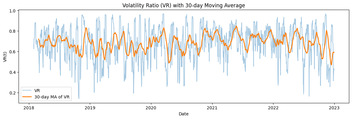
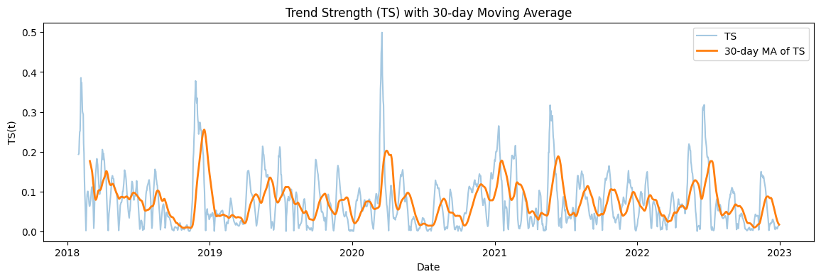
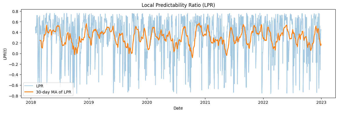
All regime–feature plots shown in the next four subsections are computed using **BTC-USD daily data from 2018 to 2023**. For reference, the corresponding **daily closing price of BTC-USD** over this period is provided below in Figure 1.

1) Volatility Ratio (VR). This measures the relative intensity of short-term volatility compared to long-term volatility:
| (1) |
where and denote rolling standard deviations over short and long windows. A rising volatility ratio typically corresponds to market stress or rapid regime shifts.
2) Trend Strength (TS). This captures the magnitude of the deviation between long- and short-term moving averages:
| (2) |
where and denote short- and long-term moving averages. Higher values indicate stronger directional trends or persistent drift in price.
3) Local Predictability Ratio (LPR). This compares short-term deviation errors against long-term deviation errors:
| (3) |
where and . Positive values imply that recent prices align more closely with short-horizon structure, indicating locally predictable behaviour.
4) Rolling Lag-1 Autocorrelation (). This quantifies the persistence or mean reversion in recent returns:
| (4) |
Positive autocorrelation suggests momentum-driven regimes, while negative values indicate mean-reversion or choppy markets.

III-B Baseline Transformer Architecture
We begin with a standard encoder–decoder Transformer operating on a fixed sequence length of tokens. Each input window of 60 historical prices is first embedded into a latent space and passed through the encoder, which consists of stacked multi-head self-attention layers followed by position-wise feedforward transformations. These layers allow the encoder to extract temporal dependencies across the full input window.
The decoder receives a start token and autoregressively generates the next price value. It applies masked self-attention to avoid peeking into the future, and cross-attention over the encoder outputs to utilize information from the input sequence. Together, this encoder–decoder design naturally models conditional forecasting tasks with flexible dependency structures.
The core of the Transformer is the scaled dot-product attention:
| (5) |
where , , and arise from learned projections of the input embeddings. This formulation defines the “baseline” attention mechanism against which our regime-aware extensions are compared.

III-C Architecture 0: Regime-Augmented Positional Encoding
In this architecture, regime information is injected directly at the input-level by modifying each token representation. The intuition is that regime dynamics—such as volatility, trend strength, predictability, and autocorrelation—represent exogenous signals that influence how the model should interpret temporal patterns. By enriching token embeddings with regime descriptors, the Transformer receives a context-aware representation before any self-attention operations occur.
Given the token embedding , positional encoding , and regime embedding , the combined representation becomes:
| (6) |
Because the Transformer is permutation-invariant, positional encodings ensure temporal ordering, while regime embeddings allow the model to distinguish between structurally different market environments. This modifies the input without altering the attention mechanism itself.

III-D Architecture 1: Regime-Modulated Attention
The motivation behind this modification is to allow the model to dynamically reshape its effective attention window depending on the current market regime. In standard self-attention, the term encodes pairwise similarity between tokens and determines which past positions each query attends to. This produces a fixed inductive behavior that does not explicitly adapt to changing market conditions.
By adding a regime-derived bias term directly inside the attention logits, we allow the model to alter these affinities in a context-dependent manner. Concretely, if the regime embedding indicates a high-volatility period, the learned projection may produce a bias that suppresses long-range attentions and strengthens short-range interactions, effectively shrinking the active receptive field. Conversely, during stable or strongly trending regimes, the bias may encourage broader temporal dependencies by amplifying attention to distant positions. The regime term acts elementwise on the pre-softmax attention matrix, analogous to a learned, input-dependent modification of the usual attention mask. Unlike a static triangular or causal mask, this regime-conditioned term can selectively boost or dampen specific rows or columns of the attention logits, thereby expanding or contracting the effective attention window on different time segments. In this way, the model can make its temporal reasoning adaptive to market structure rather than fixed across all contexts.
| (7) |
where the term serves as a regime-dependent adjustment to the standard affinity matrix. In effect, the regime operates as a dynamic mask that shifts attention weights toward or away from different temporal positions.


IV Results
IV-A Evaluation Protocol: Rolling-Origin Backtesting
To ensure realistic, forward-looking evaluation, we adopt a rolling-origin expanding-window backtesting procedure. For each asset, the historical price series is divided into multiple folds, where the training set expands forward in time while the test set moves as a non-overlapping future segment. This prevents temporal leakage and mimics how forecasting models would be deployed in practice.
We use the following rolling folds:
where each pair denotes training on the first fraction of the data and testing on the next fraction. Across all folds, predictions are concatenated to compute global metrics.
This method enables model comparison under multiple market regimes, including trending periods, sideways ranges, high-volatility phases, and sudden reversals, which is critical for evaluating regime-aware architectures.
IV-B Metrics
We evaluate all models using five widely used predictive performance metrics:
-
•
Directional Accuracy (DA): Measures the percentage of times the model correctly predicts the direction (up or down) of the next-day return. It captures a model’s trading relevance rather than raw error magnitude.
-
•
Mean Squared Error (MSE): Penalizes large errors more heavily and measures overall forecasting accuracy.
-
•
Mean Absolute Percentage Error (MAPE): Scale-normalized forecasting error measuring proportional deviation.
-
•
Pearson Correlation: Linear correlation between predicted and actual prices. Higher values indicate stronger linear agreement.
-
•
Spearman Correlation: Rank-based monotonic relationship between predicted and actual series. Useful for assessing models that capture ordinal trends rather than magnitudes.
Together, these metrics allow us to evaluate not only raw numerical accuracy (MSE, MAPE) but also forecasting structure (correlations) and trading value (DA).
IV-C Performance Summary
Table I (reproduced below) reports results for five S&P 500 tickers across the three architectures:
-
1.
Baseline Transformer
-
2.
Architecture 0 (Regime-Augmented Positional Encoding)
-
3.
Architecture 1 (Regime-Modulated Attention)
A full-page comparison table is included below.
| Stock | Baseline | Architecture 0 | Architecture 1 | |||||||||
|---|---|---|---|---|---|---|---|---|---|---|---|---|
| DA | RMSE | MAPE | Pearson | DA | RMSE | MAPE | Pearson | DA | RMSE | MAPE | Pearson | |
| AAPL | 0.5034 | 8.3701 | 9.5960 | 0.9889 | 0.5027 | 6.7371 | 7.2604 | 0.9881 | 0.4871 | 7.0646 | 7.9126 | 0.9893 |
| TSLA | 0.4979 | 36.9139 | 14.5754 | 0.9145 | 0.4940 | 31.8779 | 12.3068 | 0.9365 | 0.4933 | 32.1910 | 13.7132 | 0.9358 |
| BTC-USD | 0.4857 | 8976.3273 | 21.0792 | 0.8558 | 0.4838 | 7495.5855 | 18.0996 | 0.8998 | 0.4890 | 7547.6099 | 17.9437 | 0.8971 |
| GOOGL | 0.5003 | 7.3101 | 5.5814 | 0.9770 | 0.5115 | 6.7282 | 5.2584 | 0.9823 | 0.5027 | 6.6172 | 5.5302 | 0.9816 |
| NVDA | 0.4854 | 1.5879 | 11.8035 | 0.9773 | 0.4857 | 1.2612 | 9.5765 | 0.9865 | 0.4891 | 1.7430 | 12.1752 | 0.9807 |


IV-D Visual Comparison of Key Metrics
To provide additional interpretability, Figures 13 and 14 visualize aggregated results across all stocks for Directional Accuracy and MAPE, respectively. These two metrics summarize model performance from complementary perspectives: trend prediction (DA) and numeric precision (MAPE).


IV-E Discussion
Across nearly all stocks, the introduction of regime-awareness improves model robustness and forecasting consistency. Architecture 0 typically yields lower MAPE and higher correlation scores compared to the baseline, indicating that enriching embeddings with structural market context helps the model interpret the input sequence more effectively.
Architecture 1 further improves Directional Accuracy, suggesting that modulating attention weights based on the current regime helps the model adapt its effective receptive field. By altering the attention patterns through regime-derived biases, the model learns to focus more on short-term dependencies during high-volatility periods and to extend its temporal horizon when trends are persistent.
Overall, regime-aware mechanisms provide consistent improvements across multiple asset classes and evaluation folds, demonstrating the benefit of context-adaptive attention in financial forecasting models.
V Conclusion
This work investigated how regime-aware representations can improve the ability of Transformer models to forecast financial time series. Standard Transformers operate with a fixed attention structure, which makes them less suited for markets that frequently shift between high volatility, trending, and mean-reverting regimes. By introducing regime-driven embeddings, we allow the model to adapt its effective attention window and interpret historical prices in the context of prevailing market conditions.
Both proposed architectures—one modifying input embeddings and the other modulating attention logits—show consistent improvements over the baseline Transformer across multiple assets and evaluation metrics. These results suggest that incorporating structural market signals provides a simple yet effective way to make deep sequence models more robust to non-stationary financial behavior.
VI Acknowledgment
This project was carried out under the guidance of Prof. Amit Sethi as part of EE782: Advanced Topics in Machine Learning at IIT Bombay. We are grateful for his suggestions and discussions throughout the development of the models and experiments, which significantly helped refine the ideas presented in this work.
References
- [1] (2002) Regime changes in exchange rate volatility and uncovered interest parity. Journal of Financial Economics 66 (2-3), pp. 339–380. Cited by: §II.
- [2] (1986) Generalized autoregressive conditional heteroskedasticity. Journal of Econometrics 31 (3), pp. 307–327. Cited by: §I.
- [3] (2001) Empirical properties of asset returns: stylized facts and statistical issues. Quantitative Finance 1 (2), pp. 223–236. Cited by: §I.
- [4] (1982) Autoregressive conditional heteroskedasticity with estimates of the variance of uk inflation. Econometrica 50 (4), pp. 987–1007. Cited by: §I.
- [5] (1989) A new approach to the economic analysis of nonstationary time series and the business cycle. Econometrica 57 (2), pp. 357–384. Cited by: §I.
- [6] (2021) Rethinking positional encoding in language pre-training. In ICLR, Cited by: §I.
- [7] (2018) LogSparse transformer: logarithmic self-attention for sequential data. In NeurIPS, Cited by: §I.
- [8] (2020) Temporal fusion transformers for interpretable multi-horizon time series forecasting. In NeurIPS, Cited by: §I.
- [9] (1991) Long-term memory in stock market prices. Econometrica 59 (5), pp. 1279–1313. Cited by: §I.
- [10] (1996) The stable paretian hypothesis and the frequency of large returns: an examination of major stock indexes. Applied Financial Economics 6 (6), pp. 463–475. Cited by: §I.
- [11] (2013) On the difficulty of training recurrent neural networks. In International Conference on Machine Learning (ICML), Cited by: §II.
- [12] (2017) Outrageously large neural networks: the sparsely-gated mixture-of-experts layer. In Proceedings of the International Conference on Learning Representations (ICLR), Cited by: §II.
- [13] (2010) Analysis of financial time series. Wiley. Cited by: §I.
- [14] (2017) Attention is all you need. In Advances in Neural Information Processing Systems (NeurIPS), Cited by: §I, §II.
- [15] (2021) A transformer-based framework for multivariate time series representation learning. In Proceedings of the ACM SIGKDD International Conference, Cited by: §II.
- [16] (2021) A transformer-based framework for multivariate time series representation learning. Proceedings of KDD. Cited by: §I.
- [17] (2021) Informer: beyond efficient transformer for long sequence time-series forecasting. In AAAI, Cited by: §I.