New measurements in leptonic kaon and pion decays: experimental and theoretical perspectives
Abstract
We study the future prospects for precision measurements of purely leptonic charged-current kaon and pion decays. In particular, we consider the single ratios , for which many experimental uncertainties cancel, as well as the double ratio , which provides a particularly sensitive probe of new physics. This study is timely in light of two converging developments. On the experimental side, a new conceptual design for a dedicated setup based on a slow-extracted proton beam and a multi-year data-taking program, is expected to achieve a precision at the level. On the theory side, recent lattice-QCD calculations have reached a comparable level of accuracy. Finally, we assess the impact of these next-generation measurements on searches for physics beyond the Standard Model and show that they can provide constraints that are either competitive with or complementary to existing bounds.
1 Introduction
In the search for physics beyond the Standard Model, precision tests of SM-allowed transitions play a crucial role. Such tests, pushing the so-called intensity frontier, have been historically of great importance, for example through electroweak precision tests at LEP and SLC, and continue to play a crucial role in constraining possible new physics scenarios. Such precision SM tests are however not confined to the electroweak sector, but can be performed in complementary channels at lower energies through flavour observables.
The common argument in favour of flavour observables usually relies on accidental suppressions occurring in the SM, such as the GIM mechanism, or the conservation of lepton number, which is why flavour-changing neutral currents and lepton-flavour violating transitions are cornerstones of our exploration of the BSM landscape. In this work, instead, following the seminal proposal of [1] we want to turn our attention to charged-current decays, specifically to purely leptonic decays of light mesons, i.e. pions and kaons. These decays occur at tree-level in the SM [2, 3, 4, 5], through the exchange of a virtual boson. The only significant suppression playing a role is the helicity suppression due to the left-handed weak interaction, leading to () for .
These modes (and combinations thereof) are relevant both in our understanding of the SM, giving a clean probe of the first row of the CKM matrix, and in BSM explorations [1, 6, 7, 8, 9, 10, 11, 12, 13, 5], as they can provide important constraints on scenarios with scalar currents, or a test of lepton flavour universality complementary to those performed in and physics. This direction has also been explicitly emphasized in the recent update of the European Strategy for Particle Physics [14].
Current experimental measurements are around the per-mil level, while the SM predictions have been recently updated by lattice QCD simulations [15, 16, 17] to be well below that, at around . This new determination motivates even further the need to assess what precision could be achieved with possible future measurements of the leptonic decay rates, and what we would learn from them. We shall present a detailed analysis of both aspects, in the form of a conceptual study for an experimental setup aiming at measuring charged kaon and pion decays, and a theoretical study about the implications. The proposed programme is highly synergistic with the PIONEER experiment [18, 19], which focuses on the lepton-universality observables in pion decays. The simultaneous study of kaon and pion leptonic decays provides a unique opportunity to perform complementary and highly precise tests of lepton flavor universality, probe different effective operator structures, and enhance the sensitivity to a broad class of new-physics scenarios.
The remainder of the paper is structured as follows. In Section 2 we introduce the observables which are the focus of our study, highlighting their main features as new physics probes, alongside their current SM predictions. Section 3 contains the sketch of a new experiment, with details on the beam and detector setup, and estimates about running times and projected sensitivities for the final measurements. Following up, Section 4 is a study of our observables as BSM probes, done both within an Effective Field Theory approach and in an explicit example model. The objective is to highlight their potential in comparison to other observables, within a coherent theoretical framework. Finally, we conclude in Section 5.
2 Observables of interest
A precision flavour universality test can be performed comparing expected and measured values for the ratio
| (1) |
The experimental precision for is usually limited by systematic effects, which are primarily driven by the evaluation of absolute detection efficiencies for the positron and the muon in the final state. An attempt to partially circumvented such limitation through the exploitation of muon in flight decays to positrons is in progress at NA62, with an overall uncertainty expected to be at the level of a few per mil [20]. The present experimental state of the art is [21, 18]:
| (2) |
where the is the analogous ratio for the charged pion decays, which we report here for later convenience. On the theoretical side, recent lattice QCD determinations [15] have established
| (3) |
In a variety of new-physics scenarios, the following ratios would be affected by NP contributions as well:
| (4) |
The above ratios allow for improved cancellation of experimental systematic uncertainties. Their SM expectations derive from estimates of the ratio of decay constants and of the parameters of the CKM matrix , presently known to within a few . The current experimental values and SM predictions are 11 1 We report here only the numbers for muons, as the experimental electron ratio can be derived from the muon ratio and the double ratio. Furthermore, unlike for muons, no precise Standard Model prediction from lattice calculations currently exists for electrons [15, 16, 17], though such a calculation would be highly desirable in the future. Therefore, in our new physics studies, we will strictly use and .
| (5) |
More details on the SM value can be found in Appendix A.2. The experimental value is computed accounting for uncertainties of the and lifetimes and of the branching ratios of the two channels. The PDG averages [21] are used, as explained in Section 3.3.4.
The double ratio
| (6) |
evades from the above limitations and, while allowing a thorough cancellation of the experimental systematic effects, is also theoretically very clean. The helicity suppression is stronger for kaons than for pions by more than one order of magnitude. Consequently, NP effects mediated by scalar currents can be expected to give comparatively larger contributions in kaon decays than in pion decays. For this reason we will typically assume that only kaons are affected by NP, such that effectively, from the theoretical perspective, the substitution can be made. This will simplify the expressions for the observables significantly. The double ratio serves as useful overall normalisation for the NP search in helicity suppressed leptonic modes.
3 Experimental considerations
We consider proposing a new experimental setup to pursue precision measurements of , and the related double ratio. The idea presented here is to exploit high-intensity, slowly-extracted 400 GeV beams such as those produced for some of the experiments of the CERN north areas. For a summary of the beam parameters considered, please refer to Tab. 1.
| Parameter | Nominal value |
| Protons per pulse per second on spill on target | |
| Acceptance of secondary beam definition system | 10 sr |
| Momentum of the secondary beam | 25 GeV |
| Number of , , transmitted per proton [] | 8, 0.8, 0.8 |
| Longitudinal space allocated for beam definition | 130 m |
| , , fluxes at the detector in 4 s-long spill [] | , , |
| : : relative flux at the detector | 85% : 5% : 10% |
| Spills per year | |
| Number , tagged per year [] | , |
3.1 Beam concepts
A conceptual sketch of the beam-defining region is shown in Figure 1. After impact of the beam protons on a light-material target (Beryllium), a momentum-selected, positively-charged secondary hadron beam can be produced to be directed towards a sensitive volume located further downstream. A system of magnetic elements (one or more large-acceptance quadrupole triplets) immediately downstream of the target focuses the secondaries emitted at a given angle (not necessarily different from zero) with respect to the incoming proton beam, with an angular acceptance of . The quadrupole system focuses the beam so that a waist is ensured at the center of the momentum-selection system, located immediately downstream. The momentum selection is provided by two pairs of oppositely polarized dipole magnets upstream and downstream of a collimator: the upstream pair induces a spatial offset to the secondaries, while the second pair brings the particles back into the nominal position. The offset is momentum dependent, so that only particles of a given momentum are made to pass through the holes of the collimator. The hole extent can guarantee a 1% relative uncertainty on the momentum. All secondaries not positively charged or with momenta away from the accepted region are virtually absorbed by the collimator. At the collimator focus, a radiator system will be used to degrade and subsequently absorb the positrons while the divergence induced on the beam will be corrected for by a second quadrupole triplet (see later).
The value of the nominal momentum is critical for the proposed measurement. To detect in-flight decays in a downstream decay volume of reasonable length, a minimum angle must be ensured for the muon emission in the laboratory. After considering a number of possibilities, we propose a 25 GeV momentum. The beam momentum corresponds to decay lengths of 188 m and 1396 m for and , respectively. With a 25% (70%) probability, a muon emitted from a pion (kaon) leptonic decay moves at least 8 cm and less than 100 cm away from the beam line of flight at 25 m, so that it can be tracked. The estimated number of , , protons transmitted by the momentum-selection system slightly depends on the angle around which the secondary beam is selected.22 2 Establishing the angle value depends on a number of infrastructure considerations which are beyond the scope of the present document. For angles of 6 mrad or less we expect and transmitted per incident beam proton. The abundance of secondary protons is of the same order of that of the .
Following the momentum selection, a further system of quadrupoles must be designed to absorb the divergence induced by the first focusing and provide a parallel beam towards the decay volume, which is paramount for achieving non-destructive particle identification via Cerenkov detectors (see later). Possibly a system for sweeping the muons produced by the hadrons absorbed at the collimator and those emitted by in-flight decays might be foreseen.
We consider an overall length of 130 m allocated for beam preparation, which might also include the beam-tracking and particle-id detectors. If the beam preparation needs more longitudinal space, the proton intensity should be scaled up to maintain the flux downstream. Up to a distance of 430 m from the target to the detector region, there should not be radio-protection limitations to such operation.
The fraction of and reaching the decay volume 130 m downstream of the target are 50% and 90%, respectively. The fractional beam composition at the entrance of the detector area is : : : : .
3.2 Detector scheme
A conceptual sketch of the detector region is shown in Figure 2.
Proceeding from upstream to downstream, the detector elements are: 33 3 Depending on the beam divergence induced by the material budget of the Cerenkov detectors, the beam tracker might be placed downstream of the beam tagging system, contrary to what is presently considered.
- •
A fast beam tracker to determine the position, time, and three-momentum of each incoming beam particle. A possible implementation consists of three stations of silicon detectors: the first determines position and time of beam particles and is followed by a pair of dipoles with opposite polarities inducing a spatial offset which is a linear function of the momentum. The position measured by the second station provides a momentum measurement. A further dipole pair restores the beam particle to their original direction. Finally a third station provides the beam direction measurement. A time resolution at the level of 100–200 ps is required.
- •
Two Cherenkov detectors determine a positive and non-destructive identification of pions in the beam and, downstream of that, of kaons. The model for such detectors is the CEDAR developed for the CERN North Area experiments [22]. They are indicated as PTAG and KTAG, respectively, and provide a precise determination of the beam particle times. The distance from the KTAG to the decay volume must be kept as small as possible to prevent limitations due to the knowledge of the kaon lifetime. A time resolution at the level of 200 ps is required.
- •
A decay volume in vacuum including detectors to detect daughter particles emitted at large angles. The length of the decay volume is a crucial parameter, since it impacts on the number of observed events.
- •
A spectrometer system including gas-based tracking stations upstream and downstream of a large-bore dipole magnet, to determine position and direction of any charged decay daughter particle emitted. Centrally, it includes a non-instrumented region (“hole”) to allow passage of beam particles. In this study we considered the hole to be circular and 6 cm in radius. A relative momentum resolution at the level of 0.3% is required.
- •
A calorimeter system with capability to detect and identify positrons, pions, and muons: it should include an electromagnetic calorimeter and a muon hodoscope following a passive material block thick enough to absorb any non minimum-ionizing particle. The electromagnetic calorimeter will host a non instrumented region to allow passage of the beam particles, here considered circular and with a radius of 6 cm. The outer radius of the calorimeter must be of the order of 1.1 m. The calorimeter system will participate in the online trigger system together with the KTAG/PTAG systems, thus providing streams of data with a programmable number of daughter , , . The trigger time jitter must be reduced to within 200 ps, to limit pile-up effects.
3.3 Expected yield and sensitivity to leptonic width ratios
3.3.1 Intensity considerations
We consider a beam intensity of protons on target per second on spill, which is roughly a factor of 50 lower than that provided for a number of CERN North Area experiments [23, 24]. Considering spills with 4 s flat top, the flux of incoming , , and protons at the downstream detector per spill are: , , , respectively. Given such intensities, the setup proposed does not require to be installed in an underground area.
3.3.2 Particle fluxes at the detector
The flux of beam particles at the detector is 32 MHz, so that the probability of having an accidental beam particle to within 0.5 ns from the trigger time is 1.6%, which should limit enough pileup effects. Without a sweeping system in the beam preparation section, the flux of muons from in-flight and decays upstream of the decay volume would be approximately per spill, corresponding to an accidental matching probability of 0.2% in a 0.5 ns time window. If the secondary beam is taken at an angle larger than 6–7 mrad, the hard component of the muon flux from hadrons created in the most upstream collimator might be directed out of the acceptance of the detector, thus decreasing the needed sweeping power.
3.3.3 Trigger considerations
With a roughly 50% acceptance, the expected number of decays within a 50 m long fiducial volume is and per spill. The decays to are obviously negligible in terms of trigger bandwidth. A two-level trigger system might be considered. The level zero would be based on logical conditions applied at the hardware level through field-programmable gate arrays (FPGAs) and would include the PTAG, the KTAG and a cluster counting in the calorimeters and in the large-angle vetoes. The level-zero yield will flag more than 5 million events per spill. The level one would be software based and should run a full event reconstruction, including the tracking algorithms both for the beam and the daughter particles. The computing request for the Level 1 operation is not negligible and its infrastructure and design will need to be carefully addressed in due time. Due to data-throughput and storage considerations, we will produce two different streams at the output level:
- 1.
Will store the data in electronic format (“raw”) for all the events with positron modes and a heavily scaled-down subset for the muon modes.
- 2.
Will store all the events with muon modes in a heavily-reduced, high-level format. The format will include the track parameters for the parent and daughter particles and only high-level information for the other detectors.
Additional trigger streams will select radiative decays or events for the search for heavy neutral leptons (HNLs), to complement the main physics goal of the experiment.
3.3.4 Sensitivity expected for 1 year of data taking
In 1 year, we assume to collect 600 000 spills corresponding to tagged and tagged mesons. The measurement of the decay widths for and and of the double ratio depend on the ratio of observed decays to those expected from the number of tagged mesons, . The number of observed decays is usually restricted to decay vertices within a “fiducial” volume used for analysis optimization:
| (7) |
where is the probability for a beam particle to decay within the fiducial volume and its decay products to arrive in the sensitive volume of the tracker and the downstream forward detectors,
| (8) |
where is the distance from the tagging detector (PTAG, KTAG) to the entrance of the fiducial volume and is the length of the fiducial volume up to the decay, is the geometric acceptance (i.e. the probability that given a decay occurs in the fiducial volume, the products reach the sensitive volume of the tracker) and
| (9) |
In principle the length of the fiducial volume can be chosen differently for each of the four leptonic modes considered. Due to the different distributions of the lepton angle of emission, each of the acceptances for the four decay modes shows a different dependence on , see Figure 3.

A bayesian analysis has been performed, also accounting for the a-priori knowledge on the kaon and pion lifetime, , as well as of the branching ratio for each of the decay modes. The input parameters for and are taken from the PDG averages [21], with uncertainties already conservatively scaled up in case of internal inconsistency observed among the various measurements, see Section 5.2 of the Introduction from [21]. The input values used for the evaluation of the expected sensitivity are: GeV, GeV, , , , . The likelihood for the evaluation of the width for each decay mode is written as follows:
| (10) |
where and are the “true” total width of the parent particle and the “true” branching ratio for the channel considered and stands for the normal distribution. They are nuisance parameters, to be estimated in the fit. The quantities and are considered fixed and taken to be equal to the PDG values for all considered particles and channels. The standard deviation of is then given by
| (11) |
following the normal approximation to the binomial distribution. When evaluating the double ratio , ten terms enter the product of probabilities, related to the number of decay and branching ratio for each mode, and the total widths for the parent.
We performed two evaluations of the expected uncertainties implied by the minimization of . The default one is based on a numerical simulation of the decay paths and daughter particle emission and accounts for the geometry of the decay volume and of the tracker. An alternative analysis assumes that the acceptances are independent of the decay width and proceeds through the Fisher information matrix, defined as:
| (12) |
where are the model parameters and is the covariance matrix. For the measurement of a single leptonic width for mode , the information matrix is
| (13) |
From the expression above the covariance matrix can be written as
| (14) |
To first order, the variance of is given by
| (15) |
The relative error of the partial width is
| (16) |
The results are:
- •
At the statistical level, the ratio can be measured below . The expected relative uncertainty is shown in the left panel of Figure 4 as a function of the distances and . The optimal point is obtained with values as small as possible and values around 10 m. To achieve such a stringent level for the systematic uncertainty, we will modify the distributions of the daughter particles by weighting them so that the emitted muons from pions and kaons will overlap at the detector (tracking spectrometer, calorimeters). The available statistics is such that this optimization can be performed without limiting the measurement uncertainty to above the level of .
- •
At the statistical level, the ratio can be measured to the level of in one year. The expected relative uncertainty is shown in the right panel of Figure 4 as a function of the distances and . The optimal point is obtained with values as large as possible, while limiting to below approximately 10 m. In this case, a cancellation of the systematic uncertainties is less expensive than for the muon measurements, given that the angle of emission of the daughter positrons is broadly distributed.
- •
The uncertainty on the measurement of the double ratio is dominated by the statistics collected for the positron modes and in particular the , see Figure 5 (right). With , corresponding to 1 year of data taking, the minimum relative uncertainty is . For a collected number of tagged kaons above , the total relative error scales as , thus ensuring gains for extended data taking durations. It must be noted that, as expected, the dependence on is way weaker for the double ratio than for the single leptonic ratios.


3.4 Other observables experimentally accessible
Exploiting the full kinematic reconstruction of parent and daughter charged particles, the experiment will provide state-of-the-art sensitivities to the production of heavy neutral leptons (HNL, ) in a variety of flavour coupling patterns, via searches for the decay
| (17) |
with undergoing invisible decays or escaping the detector without interaction and . Dedicated trigger streams must be implemented for such searches with a careful optimization of the available bandwidth, both at Level 1 and for the trigger output. The selection criteria for such channels are the same used for the ratios and depend on the capability to efficiently reject the backgrounds.
We expect to have large acceptances for the radiative modes as well, so that precision measurements connected to low-energy effective constants can be performed.
4 Theoretical considerations
In this section we discuss theoretical aspects concerning the ratios and as probes of heavy BSM physics. We start by describing the low-energy parametrisation in terms of broken-phase effective operators, and how gauge symmetry restoration above the electroweak scale allows to connect to other decay channels or high-energy observables. Working in the Standard Model Effective Field Theory, we want to study the impact of the proposed measurements in terms of the effectively probed scales, first considering one operator at a time, and then performing a combined fit to all kaon (and related) data. An interesting aspect regarding the ratios lies in tests of CKM unitarity in the first row, which currently shows a slight tension between experimental measurements of , , and nuclear decays [25, 26, 27]. The tension can be lifted by a NP contribution in [28], as we shall study in detail while providing future prospects from a -level measurement.
In addition to being very sensitive probes of new physics in kaon decays, can be used as a precise test of lepton flavour universality in the - sector. As such, it provides a complementary probe to the measurements in decays, among others. Within a specific flavour assumption on the new physics couplings, , , and decays can all be related, which is what makes a very interesting measurement also in the context of heavy flavour.
Finally, the flavour of the neutrino in the final state of all the decays we consider cannot be determined, implying particularly that a new physics signal could involve a neutrino. In this case, our ratios become also a probe of lepton flavour violating effects, to compare e.g. against .
4.1 Effective Field Theory approach
Assuming that new physics lies well above the electroweak scale, an Effective Field Theory approach allows not only to parametrise all possible effects, but also to take into account the large scale separation between the new physics scale and the scale of the processes being considered. The Standard Model Effective Field Theory (SMEFT) is well-suited to parametrise any effect above the electroweak scale, while below the mass of the and bosons, effects are conveniently described in the Low-Energy Effective Field Theory (LEFT).
In the double ratio (or in ), we will always assume that new physics effects are present either in muons or electrons, separately, i.e. using it as a test of lepton-flavour universality. The ratios instead allow us to extract information about the CKM combination .
4.1.1 LEFT
The natural context to parametrise new physics effects in kaon decays is the Low-energy Effective Field Theory (LEFT). This is the theory in which all heavy Standard Model fields (, , , and ) have been integrated out, electroweak symmetry is broken, and weak interactions are described by effective dimension-six four-fermion operators. Normalising our Lagrangian as
| (18) |
the LEFT operator structures relevant for our discussion are (using the notation and conventions from [29])
| (19) |
where and , and we don’t include the tensor operator, as it does not contribute to the purely leptonic decays under consideration. As a function of the coefficients listed above, our observables can be expressed as
| (20) |
where
| (21) |
from which one observes the customary chiral enhancement of the scalar contributions with respect to the SM (vector) one. The symbols indicate radiative and isospin-breaking corrections (see Appendix A.1.1). The ratio , on the other hand, is given by
| (22) |
where stands for the SM contribution, assuming thereby no new physics contribution to the pion.
4.1.2 SMEFT
Above the electroweak scale, we define the SMEFT Lagrangian to be
| (23) |
where we use the Warsaw conventions for the effective operators [30] (see Table 2). The matching of the LEFT coefficients in Eq. (19) is given by [31]
| (24) | ||||
| (25) | ||||
| (26) | ||||
| (27) |
in the weak eigenstate basis. In order to match to the mass basis below the electroweak scale, an assumption has to be made in SMEFT about the alignment of the left-handed quark fields inside the doublets . Two common choices are up- and down alignment, i.e. the limit cases where the up quarks or respectively the down quarks are in the mass eigenstates. The other component is then given by a superposition of mass eigenstates, weighted by the CKM matrix elements as follows:
| (28) |
If, for example, we want to match the coefficient onto the SMEFT in the down-aligned basis, we would get
| (29) |
and analogous expressions for all other coefficients.
4.2 SMEFT analysis
In this section we outline the connections of our observables with other relevant observables, in the flavour sector and at higher energies. Details about the individual flavour observables are given in Appendix A. Taking SMEFT (at the electroweak scale) as a starting point, we consider the operators giving an effect in leptonic kaon decays, and match them to the LEFT. Considering for the moment only the ratio (or equivalently the double ratio , as discussed in Section 2), there are a total of 5 relevant coefficients, barring flavour multiplicities on the lepton side and quark-flavour alignment:
| (30) |
Our procedure will be the following: for each of these operators, we identify the LEFT coefficients they match onto, and then proceed to identify the most relevant observable for each of them. We do this assuming separately the up- and down-alignment of the left-handed quark doublet, as these two limiting cases lead to different and distinctive phenomenology. As we consider SMEFT coefficients defined at the electroweak scale, we only account for RG evolution within the LEFT, between the electroweak scale and the relevant scale of the process, using DsixTools [32]. The only numerically relevant running effects consist of QCD-induced self-renormalisation of scalar operators. For each process, we extract a lower bound on the new physics scale as
| (31) |
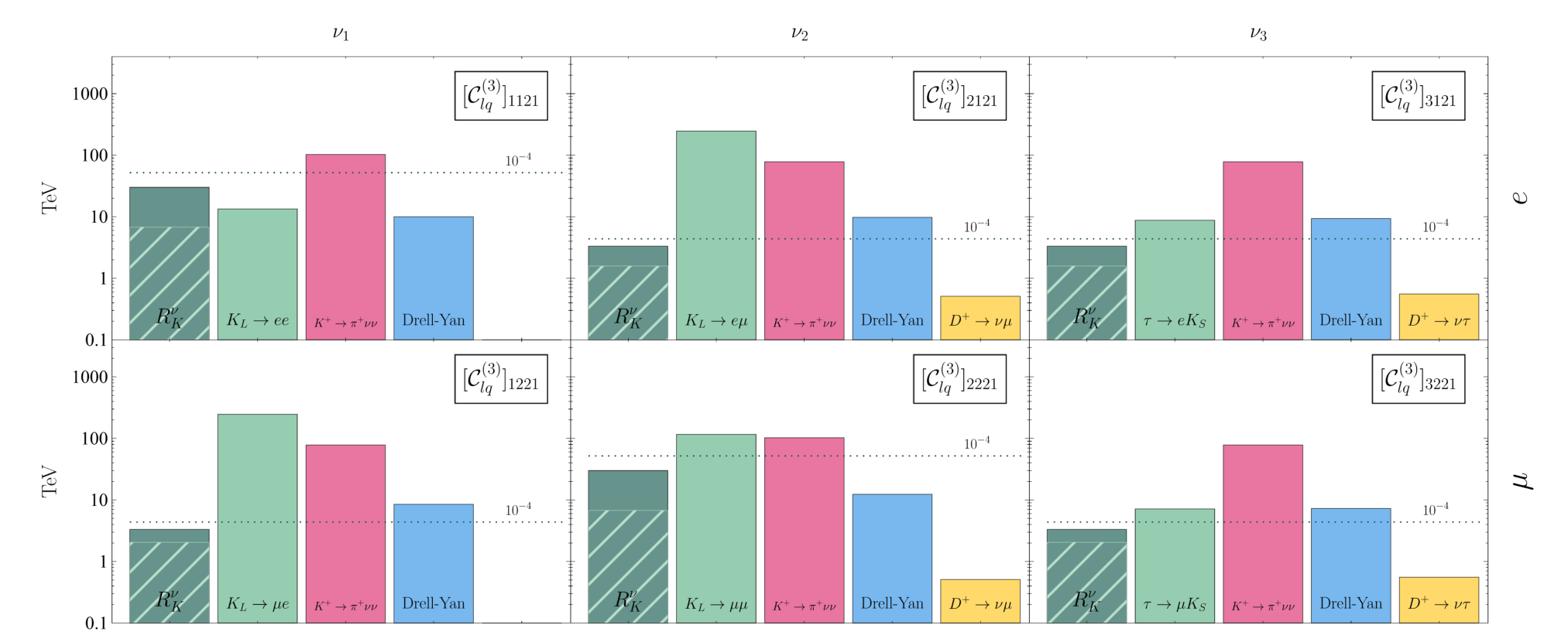
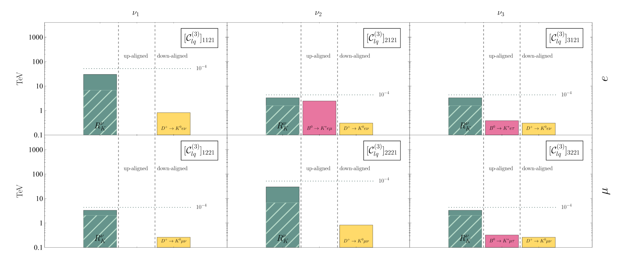
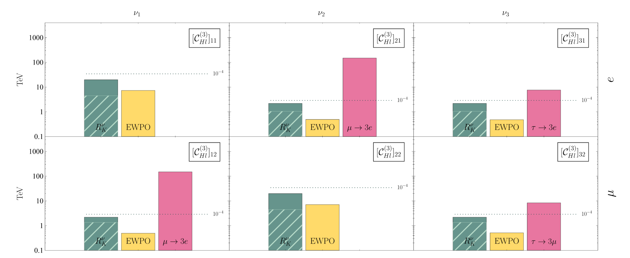
where is the 95% C.L. interval for the coefficient, assuming only one coefficient is switched on at a time. The bounds are collected in the form of bar plots in Figures fig. 6, and the numerical results in tables in Appendix B. This procedure will allow us to
- 1.
identify whether some observables may already be giving a stronger constraint than our future projection for , effectively allowing us to exclude possible new physics scenarios;
- 2.
in the opposite case, determine which observables/scenarios can be indirectly constrained by measuring leptonic kaon decays precisely.
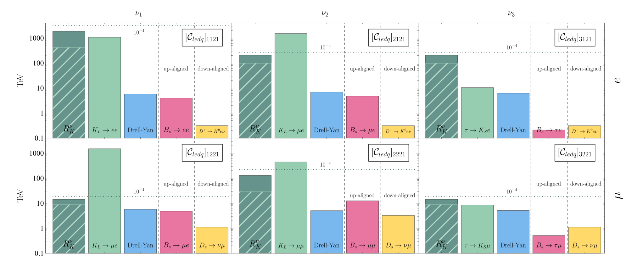
We start from . At low energies, it gives a contribution to both charged and neutral currents, since
| (32) |
where we have suppressed flavour indices. Looking in particular at , for example, we will have both a scalar and a operator, which would give a chirally-enhanced contribution to and respectively. The bounds on the new physics scale are shown in Figure 6. As can be seen, decays are today the strongest probe of , with our projections for slightly surpassing ( and will remain the dominant constraints). On the other hand, if the neutrino is assumed to be a neutrino, the rotation changing charged into neutral currents gives an expected effect in , for which is already now a dominant or competitive constraint (depending on the lepton flavour), and even more so with a future measurement. Moreover, depending on the alignment of the quark doublet, there can be additional effects in , or decays of the form or . These constraints are comparably weaker than the ones from kaon physics, which is to be expected given the additional CKM suppression, but they show an interesting interplay between , , and physics, which is unavoidable to some degree. Below we will discuss these interplays in a more concrete setting. Finally, it should be mentioned that for all flavour combinations high- Drell-Yan tails also offer complementary constraints.
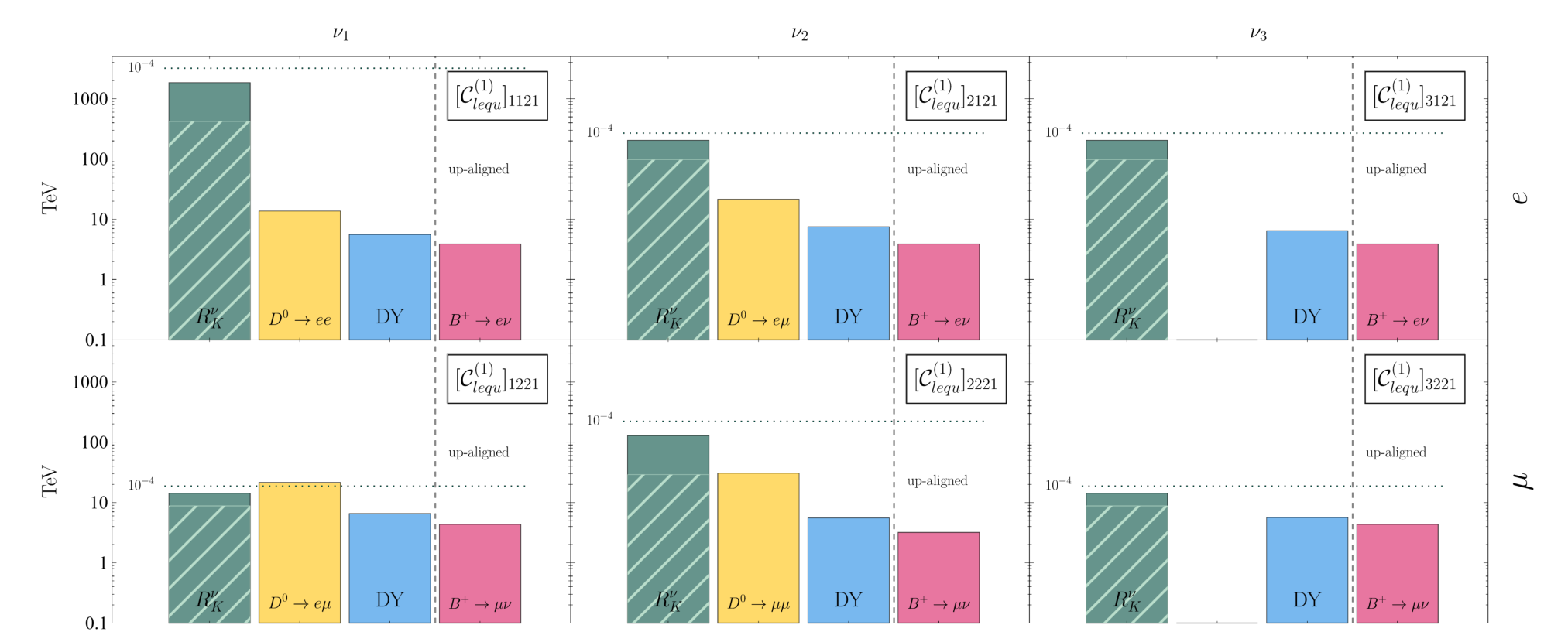
Moving to the other scalar operator in the game, the picture is somewhat simpler in this case. Similarly to before, we can expand out the quark and lepton currents to get
| (33) |
such that the charged-current kaon decays are now naturally linked to FCNCs in the charm sector, and through a flavour rotation in the case of up alignment, to charged current decays. Given the scalar structure of the operator, the more significant constraints always come from purely leptonic decays, such as , or (cf. Figure 7), but the kaon constraints tend to dominate the picture. High- Drell–Yan measurements again offer complementary constraints, which are weaker than those from .
The case of the semileptonic vector operator is the more involved one, since
| (34) |
Regarding connections in the neutral current kaon decays, our ratio is now linked to both dilepton and dineutrino final states. For muon and electron neutrinos in , the comparison with follows the same pattern as for the case. In the case of , however, provides an even stronger constraint, confirming the naive expectation that when both charged and neutral currents are present, the latter are usually the most sensitive to new physics contributions (cf. Figure 14). This also applies to the lepton-flavour violating case with tau leptons, where is stronger than . Another interesting observation is that there is not a large difference in sensitivity in between the lepton-flavour conserving and the violating case. This is due to the fact that, even in the flavour-conserving (i.e. interfering with the SM) case, the fit is dominated by the new physics contribution, which tends to be larger than the SM and have opposite sign, thus resulting again in a SM-like central value. This sort of double-solution behaviour is due to the current experimental and theoretical precisions, and has been already observed in previous works [33, 34]. The chiral enhancement also falling short in this case, Drell–Yan now plays a more important role as well, competitive with kaon decays in many cases. We also show the related constraints in the charm sector, led by . These are however comparably weaker. Similarly to the cases above, contributions from other flavour observables due to left-handed quark alignment lead to subleading contributions, and we choose to not show them here for brevity. The corresponding plots are however reported in Appendix B.
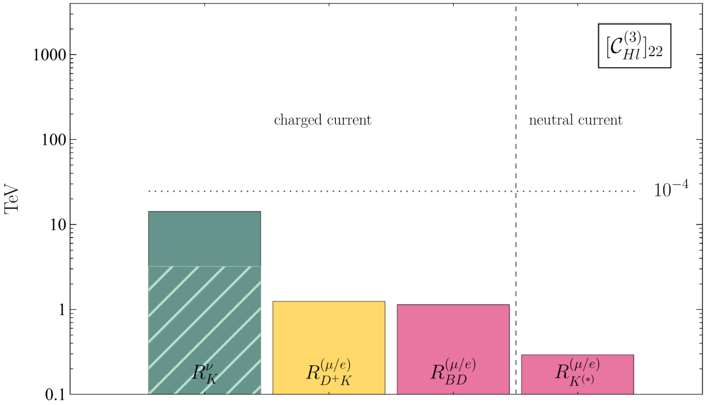
Since doesn’t affect any quark current, its effect is essentially a lepton flavour (universality) breaking one. As we can see in Figure 16, in the case of flavour-conserving currents, provides a better probe than current electroweak precision measurements. However it is important to remark that this is the only case where the single ratio differs from the double ratio as a probe of new physics. Indeed, the double ratio (which is the measurement proposed in this work) would be insensitive to , as the lepton couplings systematically cancel out. To recover the sensitivity to the lepton couplings, an improved measurement of the ratio is necessary. We postpone a more detailed discussion of the issue to Section 4.3 in the context of lepton flavour universality tests. Lepton-flavour violating indices, on the other hand, are quite effectively probed by or decays occurring through a virtual exchange.
Finally, the case of is conceptually different. Since only the couplings to quarks are affected in this case, the ratio (or, equivalently, the double ratio ) is not affected, and we need to compare our prospects for with complementary flavour observables. Drell-Yan in this case is not a very sensitive probe, as the energy-enhancement typical of four-fermion operators falls short in this case, as the SM Drell-Yan distribution is only shifted by a small constant term. In the case of flavour observables, there is a direct connection with neutral-current kaon decays such as and , which are both slightly stronger than (see Figure 17).
Global kaon fit
Having studied what happens in the case of individual coefficient fits, we now show how the constraints change assuming all of the five above coefficients are switched on at a time. This will allow us to establish to which degree the combination of kaon data, together with their SMEFT-related processes, can give us insights about generic new physics affecting the kaon sector. We do so assuming the down-aligned basis, although given the CKM suppression in heavier quark decays we find that the choice of alignment has no impact on the fit. Regarding leptonic indices, we assume new physics in muons, but very similar results can be obtained in the electron case. We show the fit results for two relevant coefficients in Figures 8 and 9, assuming two different central values for our future projections of : once keeping the current central value, and once assuming the future measurement to be SM-like. In both cases we assume an improved theory error by a factor of two (see also following section). Results are shown as 1-allowed intervals by profiling over all other coefficients in Table 2, and compared to the individual fits. Overall, the fit converges with no flat directions (cf. also the full result reported in Appendix B), and we see a significant improvement in the sensitivity, especially for the scalar operator. The tension in is related to the current anomaly in first-row CKM unitarity tests, and is discussed in further detail in the next Section. The associated effective new physics scales in the global fit range from to about 50 TeV.
and first-row unitarity
An important precision measurement of the SM is the test of CKM unitarity [36, 25, 26, 27]. In the first row of the matrix this translates to
| (35) |
which is probed to very high precision. and are determined by nuclear and kaon decays. As the current precision of those is one order of magnitude larger than the value of [36], the latter can be safely neglected in our analysis, i.e. we will consider the unitarity constraint to be . The current measurements of kaon and -decays show a deviation of from 1 for this quantity.
For we will use the combined value of super-allowed nuclear decays and neutron decays. The value of instead can be estimated by kaon decays. One option is through the measurement of , using the form factors provided by lattice QCD [4, 37, 38, 39, 40]. In addition to that the decay through the ratio allows the determination of . Using the current measurements of all the decays results in [35] (see also [27, 26])
| (36) | ||||
| (37) | ||||
| (38) |
where the “IB” component of the uncertainty refers to isospin breaking corrections. Improving the measurement of to a precision of will drastically lower the uncertainty coming from the experimental side from to . Nevertheless, the total uncertainty is dominated by lattice calculations and it would only reduce marginally, to . Still, in the case of an improvement in the theoretical errors in the future, the reduction of the uncertainty on the experimental side would prove crucial. Assuming uncertainties reduced by a factor of two for both the isospin-breaking correction and for the decay constants, one would achieve (same central values considered):
| (39) |
This improvement can also be seen in Figure 10, where we show the current estimations of and from different processes. As highlighted by our profiled fit to kaon (and related) data, new physics effects in in our setup can be effectively described by one single operator, namely . Indeed, our global fit shows that the related coefficient can be constrained very well also in the profiled fit with the other lepton-flavour conserving coefficients turned on. In Figure 9, we further compare the allowed ranges with two different assumptions for the future measurement: once with the same central value as the current measurement, and secondly with the central value being the SM value, both times assuming the improved theory uncertainty. Here one can observe two crucial things:
- (i)
In both cases the difference in precision between the individual and the profiled likelihood is nearly negligible. The ratio is isolating the problem very well.
- (ii)
With the same central value as the current measurement one could find a value of away from zero, showing again the great potential of having a precise determination of .
4.3 LFU tests
The ratio is effectively a test of lepton flavour universality in the kaon sector, measuring a possible deviation from universality in muons vs electrons. In this sense, is crucially different from the double ratio we present here. Under the assumption of leptophilic new physics (i.e. SM-like quark couplings and modified lepton couplings), the double ratio can by definition not be used as a test of lepton flavour universality, and our simplifying substitution of with the single ratio cannot be made. In order to reinterpret the double ratio as an LFU test, an improved measurement on the pion side is needed, in particular of the ratio . The measurement of this ratio is precisely the target of the PIONEER experiment at PSI, which is expected to measure it at the level [18, 19]. In the following we will assume the PIONEER result to be SM-like and with the quoted precision, which allows us to extract a precision on at the same level of the projected one for .
In recent years, LFU tests have played a crucial role in our exploration of BSM, the more prominent examples given by the -physics ratios and [41, 42, 43, 44, 45]. Here we want to compare the precision of different LFU tests in , , and decays. The quark-level transitions are all different and potentially unrelated (see next section for a common approach), but we will consider for each sector observables measuring ratios. An effective comparison can then be done by assuming that new physics modifies the lepton coupling of the and/or bosons. In practice, we will work again within SMEFT, and assume that, at the electroweak scale, NP effects can be encoded in the coefficient , i.e. we modify the and the couplings. This choice also allows us to compare charged-current and neutral-current ratios, which tend to have very different sensitivity to NP scales due to the smallness of the neutral currents in the SM. For illustration, we choose for each sector the most relevant observables, namely:
- •
kaons: for charged currents, we use the estimate for presented here. On the neutral current side, the experimental upper bound on modes is still one order of magnitude above the SM expectation, and hence no meaningful LFU test can be derived.
- •
- •
mesons: the most precise charged-current -decay ratio is , defined as
(42) for which the experimental measurement and SM expectation are [47, 48]
(43) For neutral currents, we consider the well-known ratios
(44) which are expected to be unity in the SM (with percent-level error [49, 50]), and whose experimental determinations are [51]
(45)
We show again our results in form of a bar chart indicating the NP scale associated with each LFU test in Figure 11. One can clearly see the constraining power of , as our future projection will provide the strongest test so far in this context, with effective scales reaching above 10 TeV.
4.4 Third-generation new physics
A common assumption which has risen in popularity in recent years is the idea that new physics should couple in a non-universal way to the three fermion families, with a preference for the third generation [52, 53, 54, 55, 34, 32]. This assumption allows on one hand to lower the NP scales involved (direct searches are less stringent without new physics in valence quarks), and on the other hand is a typical feature in models addressing both the Higgs hierarchy problem and the SM flavour puzzle. In our SMEFT language, this implies that, on the quark side, we need to consider only coefficients with third-generation quark fields. In particular, our SMEFT Lagrangian (at the electroweak scale) is
| (46) |
where we have ignored operators involving right-handed top quarks. Two important issues need to be addressed in this context. The first is again the question of the alignment, this time relevant only for the third-generation doublet , while the second is how we parametrise flavour-violating effects. We chose to work in the down-aligned basis, i.e. with
| (47) |
On the flavour-violating side, a -scaling of the effective coefficients is compatible with the assumption of third-generation couplings [56, 57, 58]. This is characterised by assuming a symmetry rotating the first- and second generation quark doublets into each other, at leading order. The largest effects in the breaking of this symmetry can be parametrised by the breaking spurion
| (48) |
with and of . In other words, flavour-violation is expected to follow a CKM-like structure, with deviations possible due do the assumption. Most importantly, this assumption now allows us to connect different quark-level transitions, as for example those in the LFU tests discussed in the previous section. Operationally, the effect of the spurion can be taken into account by replacing
| (49) |
in the operators listed above. After doing so, it is easy to see that our charged-current kaon decays will only be affected by the coefficient with two insertions of the spurion . , instead, enters only neutral-current processes, and the scalar operator cannot be rotated into a current, and hence will only affect -physics and high- searches. On the lepton side, we consider again muonic indices, focusing on five key observables: , , , , and . Di-neutrino modes, such as and , are affected as well. However, not knowing the neutrino flavour, one can make the assumption of new physics effects involving neutrinos, coherently with the third-generation dominance picture. This has been shown to lead to a good compatibility between flavour, high-, and electroweak precision tests with a scaling [34, 33]. Moreover, we can then use the result from said analysis to fix the values of and in our fit, effectively leaving the Wilson coefficients with light leptons as only free parameters. We thus fix and , compatibly with the results in Ref. [33], and show the constraints in the - plane in Figure 12. strikes as a very strong constraint, but it is only sensitive to one combination of coefficients. Our future expectation for probes a complementary, independent direction, effectively making charged current kaon decays into a clean precision test of third-generation NP with additional muon couplings, and surpassing the sensitivity of Drell–Yan and searches. The dashed contours in Figure 12 indicate the combined constraint, once the third relevant coefficient () has been profiled over.44 4 The region is only slightly larger than in the two-parameter fit, as leads to a chirally-enhanced contribution in . The main constraint on the vector coefficients is then given by the LFU tests , which have a similar sensitivity. The overall associated NP scale we extract from the 2 combined allowed range is
| (50) |
The results just described can also be interpreted in a -like picture on the lepton side. The leading -symmetric term only contains vector operators, with . This combination is sensitive to Drell–Yan searches with electrons and muons in the final state, and to . Note that the scalar contribution in the latter falls short, as with light lepton indices is not allowed by the symmetry. All other observables, being LFU tests, probe a breaking of . The leading term of this breaking comes from rotating third-generation indices into light ones via a spurion of the form
| (51) |
in analogy to the quark case. LFU tests, along with LFV searches, can then be used to constrain the size of [59]. A rough estimate of from can be made by considering an effective scale of approximately 1.5 TeV associated with , and the scaling . One finds
| (52) |
which is a looser constraint compared to the results in Ref. [59]. As such, should be considered as a probe of additional (non-minimal) breaking.


4.5 A simplified leptoquark model
Semileptonic interactions like the ones discussed in the SMEFT context in the previous sections can be generated in the UV by leptoquark states, which come with the additional advantage of suppressing four-quark operators and therefore meson mixing effects. We consider here the example of a scalar leptoquark, with quantum numbers under the SM gauge group. This leptoquark state has been studied extensively in the context of the -anomalies [60, 61, 62, 63], but we now want to focus on the kaon sector. The interaction Lagrangian with the SM fermion fields features two independent Yukawa coupling structures:
| (53) |
Assuming the mass of the leptoquark to be above the TeV scale, we can integrate it out and match its effects onto SMEFT, giving rise to the following contributions:
| (54) |
Since we are looking for a chiral enhancement in decays, we choose to switch on the couplings
| (55) |
which in terms of activated SMEFT coefficients at the leptoquark mass scale yields non-zero , , and . Thus, in addition to the constraints from discussed in the SMEFT analysis above, there will be additional tree-level constraints from Drell-Yan production, especially in the case of , mediated by . Moreover, working in a UV-complete setup allows us to precisely study one-loop phenomenology, the most important effect being - mixing. Working in the down-aligned basis, the main contribution to the mixing comes from the operators , generated at one loop. The structure mediating the oscillation is then obtained through the misalignment of the mass eigenstates, giving [60]
| (56) |
The most recent result from the UTfit collaboration [64] quotes
| (57) |
giving
| (58) |
Should one assume up alignment instead, the meson mixing constraint is substituted by - mixing, and on top of that a contribution to arises from the down-quark content of the doublet . The kaon mixing constraint is given by [60, 64]
| (59) |
The relevant constraints are shown in the - plane in Figure 13, where the impact of the ratio is apparent. With current data it is already competitive with or , and the future projection will make it the most relevant constraint in this sector. A comment is due regarding the Drell–Yan constraints. Given our choice of TeV, we still work in the EFT approximation and don’t consider the effect of the leptoquark -channel propagation, as this has been shown to have a small impact in this regime [65]. However, on the side, the constraints are comparably weak, since at tree-level there is no effect in neutral-current Drell–Yan, and the main effect comes from . On the side, typical scales lie in the 10 TeV range, corresponding to couplings for our choice for the mass.


5 Conclusions
A dedicated next-generation experiment measuring the kaon-to-pion leptonic decay width ratios, for electron modes and for muon modes, represents a timely opportunity for precision flavor physics. Making use of slow-extracted proton beams such as those from the CERN SPS used for a number of experiments at the CERN North Area, we have demonstrated the technical feasibility of producing and managing high-intensity secondary beams, yielding approximately tagged pions and tagged kaons per year.
Within just a few years of data taking, this setup will achieve unprecedented statistical precision: for and for . While the proposed ratios allow cancellation of experimental systematic uncertainties, their SM expectations derive from estimates of the ratio of decay constants and of the parameters of the CKM matrix , presently known to within a few .
The double ratio evades from the above limitations and, while allowing a thorough cancellation of the experimental systematic effects, it is also theoretically extremely clean and an important probe of new physics. In the experiment setup here discussed, the double ratio can be measured with total uncertainties around after few years, thus improving on the state of the art by a factor of 10 or more. Moreover, the experiment will provide state-of-the-art sensitivities to the production of heavy neutral leptons in a variety of flavour coupling patterns, improving the sensitivity on the related squared couplings.
We thoroughly reviewed the connection of , , and to other observables, both in the flavour sector and in high- and electroweak precision tests, under the assumption of heavy new physics above the electroweak scale. Starting from an EFT approach (SMEFT), we showed the constraints and relevant connections for NP affecting kaon decays. Moreover, we analysed the impact of our ratios in the context of tests of lepton flavour universality, and physics coupled mainly to the third generation, As a UV application, we showed a simplified leptoquark model, and the additional correlations arising in this case.
Ultimately, we have demonstrated that in many cases a next-generation measurement of kaon and pion leptonic decay widths with the quoted uncertainties will lead to dominant or competitive sensitivity to heavy BSM physics. In particular, the best sensitivities are obtained for chirally-enhanced scalar operators, for which scales up to 103 TeV can be probed. Also in the context of LFU tests the measurement of the double ratio, together with the prospects from PIONEER [19], will provide the leading constraint. For third-generation new physics, kaon LFU ratios will provide a useful complementary probe to current measurements. Finally, the allowed parameter space for an example leptoquark model can be probed with largely improved sensitivity.
Acknowledgements.
We would like to thank Matheus Martines and Olcyr Sumensari for helpful discussions. This project has received support from the Deutsche Forschungsgemeinschaft under Germany’s Excellence Strategy EXC 2121 “Quantum Universe” – 390833306, as well as from the grant 491245950. LT’s research is funded by the Deutsche Forschungsgemeinschaft (DFG, German Research Foundation) - Projektnummer 417533893/GRK2575 “Rethinking Quantum Field Theory”. TS would like to thank Giuseppe Ruggiero for the useful discussions.Appendix A Details on flavour observables
In this section we report further details on the flavour observables used in our fits. A list of all observables, with their current experimental determinations and SM predictions, can be found in Table 3.
| Observable | Exp. value | Ref. | SM prediction | Ref. |
| [21] | [15] | |||
| 1.3367(28) | [21] | 1.316(6) | A.2 | |
| [21] | [66] | |||
| [21] | – | |||
| [21] | [66] | |||
| [21] | [33] | |||
| [21] | [67] | |||
| [21] | – | |||
| [21] | [67] | |||
| [21] | [4] | |||
| [21] | [4] | |||
| [21] | [4] | |||
| [21] | [68] | |||
| [46] | [47] | |||
| [21] | [4] | |||
| [21] | [4] | |||
| [21] | [69] | |||
| [21] | – | |||
| [21] | [70] | |||
| [21] | – | |||
| – | ||||
| [21] | [33] | |||
| 0.995(45) | [71] | 0.9960(2) | [47] | |
| 0.95(7) | [51] | 1.00(1) | [49] | |
| 1.03(10) | [51] | 1.00(1) | [49] | |
| [21] | – | |||
| [72] | – | |||
| [73] | – | |||
| [74] | – | |||
| [74] | – |
| Parameter | Value | Ref. | |
| 0.22330 | [35] | From decays | |
| 0.97384 | [35] | From -decays | |
| 1.1932(19) | [4] | ||
| 155.7(3) MeV | [4] | ||
| 130.2(8) MeV | [4] | ||
| 190.0(1.3) MeV | [4] | ||
| 230.1(1.5) MeV | [4] | ||
| 212.0(0.7) MeV | [4] | ||
| 249.9(0.5) MeV | [4] |
A.1 Leptonic meson decays in LEFT
Using the Lagrangian 18 with the operators defined in 19 one can describe all scalar meson decays to by
| (60) |
see in Appendix A.1.1 the discussion about the radiative corrections . The decay of neutral mesons to two leptons in LEFT is mediated by the following LEFT operators,
| (61) |
where the can be replaced by either or depending on the quark content of the neutral meson. The branching ratio to two general leptons can then be written as
| (62) | ||||
| (63) | ||||
| (64) |
where
| (65) |
and
| (66) | ||||
| (67) | ||||
| (68) | ||||
| (69) |
where depending on the quark content as in 61 of the meson the is replaced by or .
A.1.1 Radiative corrections for leptonic decays
Here, we comment about the radiative corrections in 60. The universal electroweak short-distance enhancement factor for semileptonic decays in the SM [75] is at the scale for and , and at the scale for decays. The long-distance electromagnetic corrections are denoted by are channel-dependent corrections [75, 76, 77, 78, 79, 80, 81, 17, 15, 82, 83, 84, 85, 86, 87]. In the case of , they are given [75, 76, 77, 78, 79] by
| (70) |
where is the fine-structure constant and describes the leading universal long-distance radiative corrections for a point-like meson [75]
| (71) | ||||
The constant encodes hadronic structure effects calculated in Chiral Perturbation Theory (ChPT) [77, 78, 79] and drops out in the double ratios. In addition to ChPT, for has recently been evaluated using first-principles lattice QCD calculations [80, 81, 17, 15], yielding compatible results. Since lattice determination is not yet available for , we use the ChPT estimate for the electronic mode. For leptonic -meson decays, long-distance QED corrections cannot be evaluated via ChPT and are instead calculated using SCET and -meson LCDAs [82, 83, 84, 85, 86, 87], while for -meson decays first attempts are in [88].
A.2 in the Standard Model
When using for our fits to new physics, we are determining the SM value with
| (72) |
where [17] are the radiative and isospin-breaking correction. To not take the the isospin-breaking twice, the decay constants are taken uncorrected as [4]. Furthermore, we take into account the CKM elements determined from and -decays as in Tab. 4. This results in a SM value of
| (73) |
A.3 Semileptonic decays and LFU ratios
A.3.1 Di-neutrino modes
At the and mass scale, the new physics contributions to the modes can be expressed in the LEFT as
| (74) |
| (75) |
where
| (76) |
and
| (77) |
The SM values for the LEFT coefficients are
| (78) |
with [89, 90, 91, 92, 93, 94, 95, 96]
| (79) |
and the ones with right-handed quark currents are zero. In all expressions above, the Wilson coefficients contain both the SM and the new physics contribution.
A.3.2
In the charm sector we use the semi-leptonic decays [68]
| (80) |
and
| (81) |
The coefficients can be replaced by the LEFT coefficients as
| (82) | ||||
| (83) | ||||
| (84) | ||||
| (85) | ||||
| (86) |
The two branching ratios can then be combined to the LFU ratio
| (87) |
A.3.3
Another LFU ratio we consider is
| (88) |
which can be described by [47]
| (89) | ||||
| (90) |
The coefficients describe the vectorial, scalar and tonsorial coupling, which in SMEFT can be written as
| (91) | ||||
| (92) | ||||
| (93) |
A.3.4
Lastly we also considered the ratio , where
| (94) |
Assuming NP couplings only to the in the lepton sector, we can write the ratio including NP as [97]
| (95) | ||||
| (96) |
up to linear order in the Wilson coefficient, where the values of are in GeV, and
| (97) |
A.4 LFV and decays
Appendix B Additional results
In this section we report all the numerical results and additional plots which we omitted from the main text for the sake of brevity.
B.1 Individual fits
Figures 14-17 contain the single-coefficient bounds for the SMEFT operators in Table 2, except for the scalar ones. Moreover, all bounds obtained from the individual fits to the ratio are collected in Table 5. Finally, for the coefficient , to which is insensitive, we find
| (100) |
| Coefficient | lepton indices | ||||||
| 11 | 12 | 13 | 21 | 22 | 23 | ||
| current | 420 | 98 | 79 | 8.9 | 29 | 8.9 | |
| future | 1860 | 206 | 206 | 14.3 | 129 | 14.3 | |
| current | 418 | 97 | 97 | 8.8 | 29 | 8.8 | |
| future | 1850 | 205 | 205 | 14.2 | 129 | 14.2 | |
| current | 6.8 | 1.6 | 1.6 | 2.1 | 6.8 | 2.1 | |
| future | 30 | 3.3 | 3.3 | 3.3 | 30 | 3.3 | |
| current | 4.5 | 1.0 | 1.0 | 1.4 | 4.5 | 1.4 | |
| future | 19.9 | 2.2 | 2.2 | 2.2 | 19.9 | 2.2 | |

B.2 Global kaon fit
Figure 18 contains the individual and profiled fits for all six SMEFT coefficients in Table 2, with muon indices on the lepton side.

References
- (1) A. Masiero, P. Paradisi and R. Petronzio, Probing new physics through universality in , Phys. Rev. D 74 (2006) 011701 [hep-ph/0511289].
- (2) FlaviaNet Working Group on Kaon Decays collaboration, An Evaluation of and precise tests of the Standard Model from world data on leptonic and semileptonic kaon decays, Eur. Phys. J. C 69 (2010) 399 [1005.2323].
- (3) FlaviaNet Working Group on Kaon Decays collaboration, Precision tests of the Standard Model with leptonic and semileptonic kaon decays, in 5th International Workshop on e+ e- Collisions from Phi to Psi, 1, 2008 [0801.1817].
- (4) Flavour Lattice Averaging Group (FLAG) collaboration, FLAG review 2024, Phys. Rev. D 113 (2026) 014508 [2411.04268].
- (5) J. Aebischer et al., Kaon physics: a cornerstone for future discoveries, J. Phys. G 52 (2025) 100501 [2503.22256].
- (6) A. Masiero, P. Paradisi and R. Petronzio, Anatomy and Phenomenology of the Lepton Flavor Universality in SUSY Theories, JHEP 11 (2008) 042 [0807.4721].
- (7) J. Ellis, S. Lola and M. Raidal, Supersymmetric Grand Unification and Lepton Universality in , Nucl. Phys. B 812 (2009) 128 [0809.5211].
- (8) J. Girrbach and U. Nierste, in the Minimal Supersymmetric Standard Model, 1202.4906.
- (9) R.M. Fonseca, J.C. Romao and A.M. Teixeira, Revisiting the Ratio in Supersymmetric Unified Models, Eur. Phys. J. C 72 (2012) 2228 [1205.1411].
- (10) A. Abada, D. Das, A.M. Teixeira, A. Vicente and C. Weiland, Tree-level lepton universality violation in the presence of sterile neutrinos: impact for and , JHEP 02 (2013) 048 [1211.3052].
- (11) A. Abada, A.M. Teixeira, A. Vicente and C. Weiland, Sterile neutrinos in leptonic and semileptonic decays, JHEP 02 (2014) 091 [1311.2830].
- (12) M. Jung, A. Pich and P. Tuzon, Charged-Higgs phenomenology in the Aligned two-Higgs-doublet model, JHEP 11 (2010) 003 [1006.0470].
- (13) M. González-Alonso and J. Martin Camalich, Global Effective-Field-Theory analysis of New-Physics effects in (semi)leptonic kaon decays, JHEP 12 (2016) 052 [1605.07114].
- (14) J. de Blas et al., Physics Briefing Book: Input for the 2026 update of the European Strategy for Particle Physics, 2511.03883.
- (15) P. Boyle, N.H. Christ, X. Feng, T. Izubuchi, L. Jin, C.T. Sachrajda et al., First Lattice QCD Determination of Lepton-Flavor-Universality Ratios in Light-Meson Leptonic Decays, 2607.22358.
- (16) R. Di Palma, R. Frezzotti, G. Gagliardi, V. Lubicz, G. Martinelli, C.T. Sachrajda et al., Kaon radiative leptonic decay rates from lattice QCD simulations at the physical point, Phys. Rev. D 111 (2025) 114523 [2504.08680].
- (17) M. Di Carlo, D. Giusti, V. Lubicz, G. Martinelli, C.T. Sachrajda, F. Sanfilippo et al., Light-meson leptonic decay rates in lattice QCD+QED, Phys. Rev. D 100 (2019) 034514 [1904.08731].
- (18) PIONEER collaboration, Testing Lepton Flavor Universality and CKM Unitarity with Rare Pion Decays in the PIONEER experiment, in Snowmass 2021, 3, 2022 [2203.05505].
- (19) PIONEER collaboration, PIONEER: Studies of Rare Pion Decays, 2203.01981.
- (20) L. Bician and M. Koval, from NA62, in From Lattice to the Lab: Illuminating Kaon Decays, 2026, https://agenda.infn.it/event/50498/contributions/288100/attachments/147616/225451/RK_at_NA62.pdf.
- (21) Particle Data Group collaboration, Review of Particle Physics, Int. J. Mod. Phys. A 41 (2026) 2630011.
- (22) C. Bovet, S. Milner and A. Placci, The Cedar Project. Cherenkov Differential Counters with Achromatic Ring Focus, IEEE Trans. Nucl. Sci. 25 (1978) 572.
- (23) V. Andrieux, A. Berlin, N. Doshita, M. Finger, M. Finger, F. Gautheron et al., The large compass polarized solid ammonia target for drell–yan measurements with a pion beam, Nuclear Instruments and Methods in Physics Research Section A: Accelerators, Spectrometers, Detectors and Associated Equipment 1025 (2022) 166069.
- (24) NA62 collaboration, Observation of the decay and measurement of its branching ratio, JHEP 02 (2025) 191 [2412.12015].
- (25) C.-Y. Seng, D. Galviz, W.J. Marciano and U.-G. Meißner, Update on and from semileptonic kaon and pion decays, Phys. Rev. D 105 (2022) 013005 [2107.14708].
- (26) A. Ceccucci, Z. Ligeti and Y. Sakai, CKM Quark-Mixing Matrix, in Review of Particle Physics, vol. 41, p. 2630011 (2026).
- (27) E. Blucher, W.D. Marciano and G. D’Ambrosio, Vud, Vus the Cabibbo Angle, and CKM Unitarity, Particle Data Group (2026).
- (28) V. Cirigliano, W. Dekens, J. de Vries, E. Mereghetti and T. Tong, Anomalies in global SMEFT analyses. A case study of first-row CKM unitarity, JHEP 03 (2024) 033 [2311.00021].
- (29) E.E. Jenkins, A.V. Manohar and P. Stoffer, Low-Energy Effective Field Theory below the Electroweak Scale: Operators and Matching, JHEP 03 (2018) 016 [1709.04486].
- (30) B. Grzadkowski, M. Iskrzynski, M. Misiak and J. Rosiek, Dimension-Six Terms in the Standard Model Lagrangian, JHEP 10 (2010) 085 [1008.4884].
- (31) E.E. Jenkins, A.V. Manohar and P. Stoffer, Low-energy effective field theory below the electroweak scale: operators and matching, Journal of High Energy Physics 2018 (2018) .
- (32) J. Fuentes-Martin, P. Ruiz-Femenia, A. Vicente and J. Virto, DsixTools 2.0: The Effective Field Theory Toolkit, Eur. Phys. J. C 81 (2021) 167 [2010.16341].
- (33) L. Allwicher and M. Bordone, Implications of for new physics in decays, 2607.24494.
- (34) L. Allwicher, M. Bordone, G. Isidori, G. Piazza and A. Stanzione, Probing third-generation New Physics with K→¯ and B→K(*)¯, Phys. Lett. B 861 (2025) 139295 [2410.21444].
- (35) V. Cirigliano, A. Crivellin, M. Hoferichter and M. Moulson, Scrutinizing CKM unitarity with a new measurement of the K3/K2 branching fraction, Phys. Lett. B 838 (2023) 137748 [2208.11707].
- (36) P.D. Group, R.L. Workman, V.D. Burkert, V. Crede, E. Klempt, U. Thoma et al., Review of particle physics, Progress of Theoretical and Experimental Physics 2022 (2022) 083C01 [https://academic.oup.com/ptep/article-pdf/2022/8/083C01/49175539/ptac097.pdf].
- (37) JLQCD collaboration, Chiral behavior of decay form factors in lattice QCD with exact chiral symmetry, Phys. Rev. D 96 (2017) 034501 [1705.00884].
- (38) Fermilab Lattice, MILC collaboration, from decay and four-flavor lattice QCD, Phys. Rev. D 99 (2019) 114509 [1809.02827].
- (39) N. Carrasco, P. Lami, V. Lubicz, L. Riggio, S. Simula and C. Tarantino, semileptonic form factors with twisted mass fermions, Phys. Rev. D 93 (2016) 114512 [1602.04113].
- (40) PACS collaboration, K3 form factors at the physical point: Toward the continuum limit, Phys. Rev. D 106 (2022) 094501 [2206.08654].
- (41) D. Bryman, V. Cirigliano, A. Crivellin and G. Inguglia, Testing Lepton Flavor Universality with Pion, Kaon, Tau, and Beta Decays, Ann. Rev. Nucl. Part. Sci. 72 (2022) 69 [2111.05338].
- (42) G. Hiller and M. Schmaltz, Diagnosing lepton-nonuniversality in , JHEP 02 (2015) 055 [1411.4773].
- (43) D. Guadagnoli and P. Koppenburg, Lepton Flavor Violation and Lepton Flavor Universality Violation in and Decays, Ann. Rev. Nucl. Part. Sci. 73 (2023) 1 [2207.01851].
- (44) M. Bordone, G. Isidori, C. Mayer and J.-N. Toelstede, Probing lepton flavour universality with decays to final states, Eur. Phys. J. C 86 (2026) 398 [2511.05654].
- (45) M. Bordone, C. Cornella, G. Isidori and M. König, The LFU ratio in the Standard Model and beyond, Eur. Phys. J. C 81 (2021) 850 [2101.11626].
- (46) P.D. Group, P.A. Zyla, R.M. Barnett, J. Beringer, O. Dahl, D.A. Dwyer et al., Review of particle physics, Progress of Theoretical and Experimental Physics 2020 (2020) 083C01 [https://academic.oup.com/ptep/article-pdf/2020/8/083C01/34673722/ptaa104.pdf].
- (47) D. Bečirević, F. Jaffredo, A. Peñuelas and O. Sumensari, New physics effects in leptonic and semileptonic decays, Journal of High Energy Physics 2021 (2021) .
- (48) Belle collaboration, Measurement of the decay in fully reconstructed events and determination of the Cabibbo-Kobayashi-Maskawa matrix element , Phys. Rev. D 93 (2016) 032006 [1510.03657].
- (49) M. Bordone, G. Isidori and A. Pattori, On the standard model predictions for and , The European Physical Journal C 76 (2016) .
- (50) G. Isidori, D. Lancierini, S. Nabeebaccus and R. Zwicky, QED in LFU ratios: theory versus experiment, a Monte Carlo study, JHEP 10 (2022) 146 [2205.08635].
- (51) LHCb collaboration, Measurement of lepton universality parameters in and decays, Phys. Rev. D 108 (2023) 032002 [2212.09153].
- (52) L. Allwicher, C. Cornella, G. Isidori and B.A. Stefanek, New physics in the third generation. A comprehensive SMEFT analysis and future prospects, JHEP 03 (2024) 049 [2311.00020].
- (53) J. Davighi and G. Isidori, A Composite Theory of Higgs and Flavour, 2512.19650.
- (54) G. Demetriou, G. Isidori, G. Piazza and E. Pinsard, The third-generation-philic WIMP: an EFT analysis, Eur. Phys. J. C 85 (2025) 865 [2505.04708].
- (55) L. Allwicher, G. Isidori and M. Pesut, Flavored circular collider: cornering New Physics at FCC-ee via flavor-changing processes, Eur. Phys. J. C 85 (2025) 631 [2503.17019].
- (56) R. Barbieri, G. Isidori, J. Jones-Perez, P. Lodone and D.M. Straub, and Minimal Flavour Violation in Supersymmetry, Eur. Phys. J. C 71 (2011) 1725 [1105.2296].
- (57) R. Barbieri, D. Buttazzo, F. Sala and D.M. Straub, Flavour physics from an approximate symmetry, JHEP 07 (2012) 181 [1203.4218].
- (58) G. Isidori and D.M. Straub, Minimal Flavour Violation and Beyond, Eur. Phys. J. C 72 (2012) 2103 [1202.0464].
- (59) S. Covone, P. Morell and A. Tinari, Constraints on lepton-flavor mixing with third-generation new physics, Phys. Lett. B 879 (2026) 140582 [2511.15800].
- (60) V. Gherardi, D. Marzocca and E. Venturini, Low-energy phenomenology of scalar leptoquarks at one-loop accuracy, JHEP 01 (2021) 138 [2008.09548].
- (61) M. Bauer and M. Neubert, Minimal Leptoquark Explanation for the , , and Anomalies, Phys. Rev. Lett. 116 (2016) 141802 [1511.01900].
- (62) G. Hiller, D. Loose and K. Schönwald, Leptoquark Flavor Patterns & B Decay Anomalies, JHEP 12 (2016) 027 [1609.08895].
- (63) A. Angelescu, D. Bečirević, D.A. Faroughy, F. Jaffredo and O. Sumensari, Single leptoquark solutions to the -physics anomalies, Phys. Rev. D 104 (2021) 055017 [2103.12504].
- (64) UTfit collaboration, Constraints on new physics from the quark mixing unitarity triangle, Phys. Rev. Lett. 97 (2006) 151803 [hep-ph/0605213].
- (65) L. Allwicher, D.A. Faroughy, M. Martines, O. Sumensari and F. Wilsch, On the EFT validity for Drell–Yan tails at the LHC, Eur. Phys. J. C 85 (2025) 463 [2412.14162].
- (66) M. Hoferichter, B.-L. Hoid and J. Ruiz de Elvira, Improved Standard-Model prediction for , JHEP 04 (2024) 071 [2310.17689].
- (67) G. Burdman, E. Golowich, J.L. Hewett and S. Pakvasa, Rare charm decays in the standard model and beyond, Phys. Rev. D 66 (2002) 014009 [hep-ph/0112235].
- (68) D. Bečirević, M. Martines, S. Rosauro-Alcaraz and O. Sumensari, Interpreting the results on exclusive modes, Phys. Lett. B 880 (2026) 140713 [2603.25837].
- (69) C. Bobeth, M. Gorbahn, T. Hermann, M. Misiak, E. Stamou and M. Steinhauser, in the Standard Model with Reduced Theoretical Uncertainty, Phys. Rev. Lett. 112 (2014) 101801 [1311.0903].
- (70) M. Beneke, C. Bobeth and R. Szafron, Power-enhanced leading-logarithmic QED corrections to , JHEP 10 (2019) 232 [1908.07011].
- (71) Belle Collaboration collaboration, Measurement of the decay in fully reconstructed events and determination of the cabibbo-kobayashi-maskawa matrix element , Phys. Rev. D 93 (2016) 032006.
- (72) K. Hayasaka et al., Search for Lepton Flavor Violating Tau Decays into Three Leptons with 719 Million Produced Tau+Tau- Pairs, Phys. Lett. B 687 (2010) 139 [1001.3221].
- (73) Belle-II collaboration, Search for lepton-flavor-violating -→ -+- decays at Belle II, JHEP 09 (2024) 062 [2405.07386].
- (74) Belle, Belle-II collaboration, Search for lepton-flavor-violating decays at Belle and Belle II, JHEP 08 (2025) 092 [2504.15745].
- (75) W.J. Marciano and A. Sirlin, Radiative corrections to pi(lepton 2) decays, Phys. Rev. Lett. 71 (1993) 3629.
- (76) M. Finkemeier, Radiative corrections to pi(l2) and K(l2) decays, Phys. Lett. B 387 (1996) 391 [hep-ph/9505434].
- (77) V. Cirigliano and I. Rosell, Two-loop effective theory analysis of pi (K) — e anti-nu/e [gamma] branching ratios, Phys. Rev. Lett. 99 (2007) 231801 [0707.3439].
- (78) V. Cirigliano and I. Rosell, pi/K — e anti-nu(e) branching ratios to O(e**2 p**4) in Chiral Perturbation Theory, JHEP 10 (2007) 005 [0707.4464].
- (79) V. Cirigliano and H. Neufeld, A note on isospin violation in Pl2(gamma) decays, Phys. Lett. B 700 (2011) 7 [1102.0563].
- (80) D. Giusti, V. Lubicz, G. Martinelli, C.T. Sachrajda, F. Sanfilippo, S. Simula et al., First lattice calculation of the QED corrections to leptonic decay rates, Phys. Rev. Lett. 120 (2018) 072001 [1711.06537].
- (81) A. Desiderio et al., First lattice calculation of radiative leptonic decay rates of pseudoscalar mesons, Phys. Rev. D 103 (2021) 014502 [2006.05358].
- (82) C. Cornella, M. Ferré, M. König and M. Neubert, The simplest B decay, precisely, JHEP 06 (2026) 027 [2601.14361].
- (83) C. Cornella, M. Ferré, M. König and M. Neubert, QED Corrections to , 2607.13144.
- (84) C. Cornella, M. König and M. Neubert, Structure-dependent QED effects in exclusive B decays at subleading power, Phys. Rev. D 108 (2023) L031502 [2212.14430].
- (85) M. Beneke, P. Böer, J.-N. Toelstede and K.K. Vos, QED factorization of non-leptonic decays, JHEP 11 (2020) 081 [2008.10615].
- (86) D. Becirevic, B. Haas and E. Kou, Soft Photon Problem in Leptonic B-decays, Phys. Lett. B 681 (2009) 257 [0907.1845].
- (87) P. Böer and T. Feldmann, Structure-dependent QED effects in exclusive -meson decays, Eur. Phys. J. ST 233 (2024) 299 [2312.12885].
- (88) T. Kitahara, J. Miyamoto and K. Sasaki, Complete one-loop QED corrections to leptonic decays and impact on the CKM unitarity test, JHEP 05 (2026) 041 [2511.22383].
- (89) G. Buchalla and A.J. Buras, The rare decays , and : An Update, Nucl. Phys. B 548 (1999) 309 [hep-ph/9901288].
- (90) J. Brod and M. Gorbahn, Electroweak Corrections to the Charm Quark Contribution to K+ — pi+ nu anti-nu, Phys. Rev. D 78 (2008) 034006 [0805.4119].
- (91) A.J. Buras, M. Gorbahn, U. Haisch and U. Nierste, Charm Quark Contribution to at Next-to-Next-to-Leading Order, JHEP 11 (2006) 002 [hep-ph/0603079].
- (92) J. Brod, M. Gorbahn and E. Stamou, Two-Loop Electroweak Corrections for the Decays, Phys. Rev. D 83 (2011) 034030 [1009.0947].
- (93) J. Brod, M. Gorbahn and E. Stamou, Updated Standard Model Prediction for and , PoS BEAUTY2020 (2021) 056 [2105.02868].
- (94) G. Isidori, F. Mescia and C. Smith, Light-quark loops in K — pi nu anti-nu, Nucl. Phys. B 718 (2005) 319 [hep-ph/0503107].
- (95) E. Lunghi and A. Soni, Light quark loops in from vector meson dominance and update on the Kaon Unitarity Triangle, JHEP 12 (2024) 097 [2408.11190].
- (96) F. Mescia and C. Smith, Improved estimates of rare K decay matrix-elements from Kl3 decays, Phys. Rev. D 76 (2007) 034017 [0705.2025].
- (97) C. Cornella, D.A. Faroughy, J. Fuentes-Martín, G. Isidori and M. Neubert, Reading the footprints of the b-meson flavor anomalies, Journal of High Energy Physics 2021 (2021) .
- (98) I. Plakias and O. Sumensari, Lepton flavor violation in semileptonic observables, Phys. Rev. D 110 (2024) 035016 [2312.14070].