A Systematic Comparison of Multilingual Interpretability Methods
Reveals Anisotropy-Driven Failures

Oskar Holmström Marcel Bollmann Marco Kuhlmann Affiliation: Linköping University Email: oskar.holmstrom@liu.se

Abstract

Multilingual language models develop shared cross-lingual representations, and various interpretability methods claim to quantify this sharing. These methods have been developed largely in isolation, and when they disagree, it is unclear whether the disagreement reflects a property of the model or an artifact of the measurement. We compare four sharing metrics —CKA, ANC, GMM dominance per token, and ILO —across 21 base models from five families (125M–14B parameters) and correlate each with cross-lingual transfer on five downstream tasks. We find that the metrics differ in their quantification of cross-lingual sharing in these models and suggest that the disagreement traces to anisotropy, the tendency of representations to cluster in a narrow cone of the embedding space. Only ILO’s correlation with cross-lingual transfer (Spearman’s $\rho=0.90$ ) survives controls for model size, family, and per-task variation. We therefore recommend ILO as the primary sharing metric, to be reported alongside anisotropy diagnostics.

Figure 1: Sentence embeddings at layer 18 of Qwen3-8B-Base, projected to 2D via PCA. Left: Embeddings exhibit anisotropy in that they form a narrow cone offset from the origin. Right: Removing the top-2 principal components yields a significantly more isotropic residual. We show that language identity is largely relocated to this residual (§4.2), implying that sharing metrics that explicitly or implicitly focus on the principal subspace will be unreliable.

1 Introduction

Multilingual language models develop shared representations across languages without explicit alignment supervision (Pires et al., 2019; Wu and Dredze, 2019). A growing set of interpretability methods now claims to measure this sharing: probing classifiers, similarity metrics, distributional approaches, and neuron-level analyses. These methods have largely been developed in isolation, on one or two model families at a time. When different metrics on different models yield different conclusions, it is unclear whether the disagreement reflects genuine differences between models or is an artifact of the measurement itself.

This ambiguity is especially concerning as contextual embeddings often exhibit anisotropy: they occupy a narrow cone in the representation space, rather than spreading evenly in all directions (isotropy), with variance concentrated in a few dimensions (Ethayarajh, 2019; Timkey and van Schijndel, 2021), as shown in Figure 1. Anisotropy poses at least two risks for any geometric measure of cross-lingual sharing: First, it inflates apparent similarity, making any two vectors look close by default. Second, it confines meaningful variation to a low-dimensional subspace, so any metric sensitive to dominant directions of variance —whether it explicitly projects onto them or implicitly up-weights them —will be driven by that subspace rather than by the full representational geometry.

Because conclusions about which architectures, training regimes, and scaling choices yield stronger cross-lingual sharing are only as reliable as the metrics on which they rest, it matters whether metrics can be trusted to track sharing through anisotropy. This paper therefore examines how this distortion affects the metrics under consideration, and assesses which, if any, can be relied on to reflect genuine cross-lingual sharing.

Concretely, we address three questions through a systematic comparison of four sharing metrics across 21 base models from five families (BLOOM, OPT, XGLM, Qwen3, SmolLM3; 125M–14B parameters), supplemented by instruction-tuned variants and intermediate checkpoints:

•

How do multilingual models share representations across languages?
•

When do existing metrics agree or disagree as to the degree of cross-lingual sharing?
•

Which metric best predicts cross-lingual transfer?

Our answers, anticipating §4: models exhibit three sharing patterns rather than a binary split implied by metrics dominated by high-variance directions, and the metric disagreement traces directly to anisotropy, with language probes showing that language identity is relocated to the directions such metrics discard or down-weight. Among the four metrics, ILO (Wilie et al., 2025) is the only one whose association with cross-lingual transfer survives controls for size, family, and per-task variation, reaching a Spearman rank correlation of $\rho=0.90$ ; ANC (Del and Fishel, 2022) forms a clear second tier whose association rests on between-family contrasts, while PCA-based GMM dominance per token (Shani and Basirat, 2025) has a within-family signal too weak to characterize as a relationship across matched architectures and CKA (Kornblith et al., 2019) shows no association at any level. We therefore recommend ILO as the primary sharing metric, and further suggest that it should be reported alongside anisotropy diagnostics.

2 Related Work

Measuring cross-lingual sharing

Multilingual models develop shared representations between languages without explicit alignment supervision (Pires et al., 2019; Wu and Dredze, 2019). The contributing factors remain debated; shared positional embeddings, similar word order, parameter sharing across languages, and training-data imbalance have all been proposed as drivers (Dufter and Schütze, 2020; Conneau et al., 2020b; Schäfer et al., 2024).

A series of measures has been developed to quantify cross-lingual sharing: Similarity-based metrics compare activation patterns across languages on parallel input. Centered Kernel Alignment (CKA; Kornblith et al., 2019) measures global geometric similarity between cross-lingual representation matrices. Average Neuron Correlation (ANC; Del and Fishel, 2022) captures per-neuron alignment. Lens-based methods such as the logit lens (nostalgebraist, 2020) project intermediate hidden states into the vocabulary. Wendler et al. (2024) use this to argue that Llama-2 routes multilingual inputs through English-aligned representations. Subsequent work has questioned both the technique (Belrose et al., 2025) and the claim itself: apparent reliance on English varies with training data balance, and representations often mix from several languages rather than being pivoted toward English (Zhong et al., 2025; Schut et al., 2025; Trinley et al., 2025; Harrasse et al., 2026). Shani and Basirat (2025) present a mixture model-based metric: they fit Gaussian mixture models over PCA-projected representations and use them to derive language dominance scores. Wilie et al. (2025) introduce Interlingual Local Overlap (ILO), a neighborhood-based metric that operates on the full hidden state. Finally, neuron-level analyses identify units that activate selectively per language, using activation entropy (Tang et al., 2024; Kojima et al., 2024), ternary classifications (Zhang et al., 2026), sparse autoencoders (Deng et al., 2025), or transcoders (Harrasse et al., 2026).

A parallel line of work scores each language by its directed alignment with English and validates it against downstream performance, at the language level in MEXA (Kargaran et al., 2025) and at the instance level in DALI (Ravisankar et al., 2026). These primarily measure alignment with English rather than sharing among all languages, which is what the four metrics we compare quantify; we relate the two views in Appendix C.4. All of these methods have largely been developed and evaluated in isolation. Comparisons typically restrict themselves to one or two model families, leaving open whether disagreements between metrics reflect substantive differences between models or measurement artifacts. Filling this gap, we compare four representative metrics —spanning similarity-based, distributional, and neighborhood approaches —on the same set of models (§4).

Representational anisotropy

Contextual embeddings from transformer models tend to occupy a narrow cone in representation space rather than filling it isotropically, with most pairs of vectors having high cosine similarity regardless of their semantic content (Ethayarajh, 2019; Gao et al., 2019). Biś et al. (2021) argue that much of this apparent anisotropy stems from a common shift shared across embeddings: once the mean is subtracted, the residual distribution is closer to isotropic. Other proposed causes of anisotropy include self-attention dynamics (Godey et al., 2024) and optimizer-level effects in Adam (Stollenwerk and Stollenwerk, 2025). Regardless of cause, anisotropy distorts geometric analyses of representations. Rajaee and Pilehvar (2022) and Hämmerl et al. (2023) document anisotropy in multilingual models specifically, and show that post-hoc isotropy enhancement improves cross-lingual semantic similarity —indicating that anisotropy can mask genuine cross-lingual structure. How isotropy should be measured is itself contested (Rudman et al., 2022), and anisotropy is not uniformly harmful: it has limited impact on sentence-representation expressiveness for clustering (Ait-Saada and Nadif, 2023), is incompatible with cluster structure by construction (Mickus et al., 2024), and decreasing isotropy during finetuning can improve downstream performance (Rudman and Eickhoff, 2024). Our concern is not whether anisotropy is desirable in a model, but what it does to the metrics used to measure cross-lingual sharing (§4.2); our own diagnosis there rests on effective dimensionality and probing rather than on the cosine diagnostic alone.

3 Experimental Setup

In our main experiments, we compute four cross-lingual sharing metrics across 21 models. This section presents these metrics and models along with the data we used and our statistical framework.

3.1 Sharing Metrics

We select one metric from each of the main methodological families of representation-level cross-lingual analysis, so that the comparison contrasts kinds of measurement rather than variants of one kind: CKA for global geometric similarity, ANC for neuron-level correspondence, $\lambda$ for distributional structure, and ILO for local neighborhood overlap. The metrics are:

•

(Linear) CKA (Centered Kernel Alignment; Kornblith et al., 2019) is the established geometric-similarity baseline. It measures the similarity between two representation spaces by comparing their pairwise distance structures —specifically, how consistently pairs of representations that are similar in one space are also similar in the other. Values range from 0 (no shared structure) to 1 (identical up to isotropic scaling and orthogonal transformation).
•

ANC (Average Neuron-Wise Correlation; Del and Fishel, 2022) measures whether individual neurons carry consistent activation patterns across languages —in contrast to CKA, which measures whether the overall pairwise similarity structure is preserved across representations. For each neuron, ANC computes the absolute Pearson correlation between its activations on parallel sentences in two languages. Averaging over neurons yields a value in $[0,1]$ , where 1 indicates that every neuron responds identically (up to sign differences) across languages.
•

GMM dominance per token. Shani and Basirat (2025) fit a supervised Gaussian Mixture Model in a PCA subspace retaining 98% of variance and report the fraction of tokens whose likelihood is higher in a foreign-language space than in their own. We refer to this quantity as $\lambda$ and report it by layer after subsampling each language to 10,000 tokens before PCA and GMM fitting. This matches the subsampling used for ILO and removes tokenizer-fertility bias as a confound when comparing across families with different scripts. Unbalanced word-level and sentence-level variants appear in Appendix A.2.
•

ILO (Interlingual Local Overlap; Wilie et al., 2025) quantifies cross-lingual sharing via $k$ -nearest-neighbor queries ( $k=5$ ) in the full representation space, combining bridge scores (how often a token’s neighbors include other languages) and reachability scores (the fraction of other languages that appear in the $k$ -nearest-neighbor set of any token of that language) into a single index ranging from 0 (complete separation) to 1 (complete sharing). We compute ILO on token-level representations with the same 10,000-tokens-per-language subsample as $\lambda$ , which controls tokenizer fertility. The released implementation of Wilie et al. (2025) instead operates on mean-pooled sentence embeddings; we report that variant in Appendix B.5. We additionally report a centered variant (ILO_c), computed identically after subtracting the per-layer mean hidden state across all tokens and languages, which removes anisotropy-driven neighborhood structure that can inflate apparent sharing.

3.2 Models

Our 21 base models come from five model families, spanning 125M to 14B parameters and varying in training data composition and scale. We briefly introduce the model families here; see Appendix A.1 for full details on models and checkpoints.

•

BLOOM BigScience Workshop et al. (2023) (560M–7.1B) is trained on 350B tokens of the ROOTS corpus Laurençon et al. (2022). It covers 46 natural languages with ca. 70% non-English data, and provides pretraining checkpoints.
•

XGLM Lin et al. (2022) (564M–7.5B) is trained on 30 languages drawn from CC100-XL. We use both BLOOM and XGLM despite their age because the sharing metrics we evaluate were validated on these families: Shani and Basirat (2025) report $\lambda$ on BLOOM and Del and Fishel (2022) report ANC on XGLM.
•

OPT Zhang et al. (2022) (125M–6.7B) serves as our non-multilingual baseline. It is trained on 180B predominantly English tokens from the Pile Gao et al. (2020), BookCorpus, and CC-News, with only incidental non-English content from Common Crawl.
•

Qwen3 Yang et al. (2025) (0.6B–14B) provides a modern high-compute comparison. It is trained on ca. 36T tokens spanning 119 languages and dialects, though exact proportions are undisclosed.
•

SmolLM3 Bakouch et al. (2025) (3B) is trained on 11.2T tokens drawn primarily from FineWeb-Edu, FineWeb-2, and DCLM, with ca. 12% multilingual web data natively supporting six languages (English, French, Spanish, German, Italian, Portuguese) plus additional training on Arabic, Chinese, and Russian; it uniquely provides intermediate checkpoints across three training stages for studying multilingual representations during pre- and post-training.

We additionally characterize instruction-tuned variants —BLOOMZ Muennighoff et al. (2023), Qwen3 non-Base, SmolLM3-Instruct —and 59 intermediate checkpoints from BLOOM and SmolLM3, yielding a total of 32 model configurations plus checkpoints. Instruction-tuned variants contribute to representational characterization but are excluded from transfer analysis; all transfer correlations are based on the 21 base models. This is because our transfer protocol finetunes on English data and evaluates zero-shot (§3.4), measuring what the pretraining geometry makes possible; on instruction-tuned variants it would entangle sharing with post-training recipes that differ across families. The question we do ask about post-training—whether it changes the sharing structure—is addressed in §4.4.

3.3 Data

All interpretability analyses use the FLORES-200 NLLB Team et al. (2022) devtest set, providing 1,012 parallel sentences across ten languages: Arabic, Chinese, English, French, German, Japanese, Portuguese, Russian, Spanish, and Turkish. These languages span four scripts (Latin, Cyrillic, Arabic, CJK), multiple typological families (Romance, Germanic, Turkic, Japonic, Sino-Tibetan, Semitic, Slavic), and a range of morphological types (isolating, fusional, agglutinative). Sentence-level pairs are required by CKA and ANC, which compute cross-lingual similarity from aligned representations; the remaining methods operate on monolingual representations.

3.4 Cross-Lingual Transfer Evaluation

We use zero-shot cross-lingual transfer as a functional validation criterion, not as ground truth for sharing: transfer has drivers beyond representational alignment, among them task format, vocabulary overlap, and target-language pretraining exposure, which is why we average over five tasks, require associations to survive a number of controls (§3.5), and keep the diagnosis of the disagreement between methods (§4.2) independent of transfer.

We fine-tune each of the 21 base models on English training data and evaluate zero-shot on up to nine non-English languages (coverage varies by task; Appendix A.5) across five tasks: Belebele (reading comprehension; Bandarkar et al., 2024), XNLI (natural language inference; Conneau et al., 2018), XCSR (commonsense reasoning; Lin et al., 2021), SIB-200 (topic classification; Adelani et al., 2024), and XQuAD (extractive question answering; Artetxe et al., 2020). As an aggregate per-model metric, we compute, for each task, the mean accuracy over the non-English target languages that task covers, and then take the unweighted mean of these five per-task means. We refer to this number as the transfer score.

For each model–task pair, we sweep over 3–5 learning rates between $5\times 10^{-6}$ and $10^{-4}$ , with ranges adapted to the model family’s stable regime. We use AdamW with linear warmup (10% of steps), weight decay 0.01, and gradient clipping at 1.0. Task-specific epoch counts range from 3 to 20. The best learning rate is selected for each model–task pair based on validation accuracy. Full hyperparameters are in Appendix A.6.

Because the §4.3 correlations link base model metrics to finetuned model behavior, we re-apply the full interpretability suite after finetuning to verify that the base model geometry survives.

3.5 Statistical Framework

Beyond characterizing representations, we test for functional relevance: whether sharing metrics correlate with cross-lingual transfer, and whether any association survives controls for model size, family membership, and task choice.

Primary correlation

We use Spearman rank correlations ( $\rho$ ) for all tests. The primary correlation is computed across all models relative to the transfer score defined in §3.4.

Decompositions

We report three additional analyses to check whether the primary correlation is robust. Per-family $\rho$ separates between- from within-family contributions to the cross-model association. Per-task $\rho$ for each metric against each task (4 metrics $\times$ 5 tasks $=$ 20 tests) shows whether the primary correlation holds task by task. Because running 20 tests simultaneously inflates the family-wise false-positive rate, we apply the Benjamini and Hochberg (1995) procedure, which bounds the expected proportion of false discoveries among reported associations at $\alpha=0.05$ . This ensures that a pattern such as a correlation being significant across all five tasks reflects a consistent relationship rather than accumulated chance.

Partial Spearman $\rho$ controlling for $\log_{10}$ parameter size checks that the sharing–transfer association is not reducible to a model-size effect. Within most families, parameter count correlates with both cross-lingual sharing and transfer performance, raising the possibility that any observed association between sharing and transfer is a spurious consequence of larger models doing everything better rather than a genuine relationship between the two. Partialling out $\log_{10}$ parameters removes the variance in both sharing and transfer that is attributable to size, so that the residual correlation reflects whether sharing predicts transfer over and above what model size alone would explain.

Permutation tests

Given our small sample size, we verify significance with non-parametric permutation tests. Each test recomputes $\rho$ on 10,000 random shuffles of the transfer score values to estimate the null distribution, from which we compute a one-tailed $p$ -value as the proportion of recomputed $\rho$ values greater than or equal to the observed $\rho$ . We run two designs: The first shuffles across all models, testing whether any monotonic association exists. The second shuffles within each family only, testing whether the association persists once between-family contrasts are removed. Family membership is otherwise a confound: model families differ systematically in both architecture and training data, so the cross-model correlation could be driven entirely by between-family contrasts.

3.6 Additional Diagnostics

In addition to the sharing metrics, we report two diagnostics at each layer. Effective dimensionality ( $n_{\text{pca}}$ ) is the number of PCA components needed to retain 98% of variance; small values relative to the full number of dimensions indicate that representations occupy a low-dimensional subspace. Mean random cosine similarity is the average cosine between 5,000 random pairs of hidden states; high values indicate the “narrow cone” geometry where any two vectors look similar by default (Ethayarajh, 2019), biasing similarity-based measures upward. Together, these metrics flag layers where sharing metrics should be interpreted with caution.

4 Results and Discussion

This section presents our main results together with additional analyses, and discusses our findings. We organize the section around four questions:

4.1 How Do Models Share Representations Across Languages?

When we apply the four metrics across our 21 base models, three distinct sharing patterns emerge (cf. Table 1, Figure 2).

•

Pattern 1: Concentrated sharing (BLOOM ${\geq}$ 1B, Qwen3, SmolLM3): high $\lambda$ ( $>0.75$ ), high ILO, and variance concentrated in just $n_{\text{pca}}=2$ dimensions at the peak $\lambda$ layer. The sharing metrics increase through the middle layers and fall toward the output, producing the inverted-U profile visible in Figure 2.
•

Pattern 2: Distributed sharing (XGLM): high ILO ( $0.44$ at 4.5B, comparable to BLOOM-7.1B’s $0.40$ ) but near-zero $\lambda$ , with variance distributed across thousands of dimensions ( $n_{\text{pca}}$ in the thousands at every layer).
•

Pattern 3: Minimal sharing (OPT): low values on every metric, consistent with OPT’s predominantly English training data.

The critical case is XGLM. GMM dominance per token used in isolation groups XGLM with OPT, despite XGLM’s transfer score ( $0.55$ ) approaching BLOOM-7.1B ( $0.60$ ) and clearly exceeding OPT-6.7B ( $0.41$ ). The remaining metrics tell a coherent story: across all 21 models, ANC spans $0.34$ – $0.68$ and tracks the sharing patterns, while CKA falls in a narrow band ( $0.58$ – $0.73$ ) and discriminates poorly across families. Results for all models and metrics are presented in Appendix B.1.

Model	$\lambda$	ILO	CKA	ANC	Xfer	$n_{\text{pca}}$	$\overline{\cos}$
	Sharing					Anisotropy
BLOOM-560M	.21	.25	.66	.38	.44	20	.86
BLOOM-7.1B	.79	.40	.68	.44	.60	2	.95
OPT-6.7B	.03	.15	.58	.35	.41	3477	.99
XGLM-4.5B	.03	.44	.66	.56	.55	1702	.90
Qwen3-8B	.90	.63	.63	.66	.67	2	.99
SmolLM3-3B	.89	.70	.73	.68	.65	2	.99

Table 1: Cross-lingual sharing metrics for representative models (one per sharing pattern). Sharing metrics:

\lambda

= GMM dominance per token at peak layer; ILO = peak interlingual local overlap; CKA and ANC = mean across layers and language pairs; Xfer = transfer score (§3.4). Anisotropy diagnostics:

n_{\text{pca}}

= PCA components retained at 98% variance at the model’s peak-sharing layer(Appendix B.2);

\overline{\cos}

= mean cosine similarity between random hidden states. Full sharing results are in Appendix B.1 and anisotropy diagnostics are in Appendix B.2.

Figure 2: Layer-wise cross-lingual sharing profiles for four representative models (one per sharing pattern). Each panel shows GMM

\lambda

(dashed) and ILO (solid) according to the scale on the left and effective PCA dimensionality

n_{\text{pca}}

(dotted gray) according to the (log) scale on the right.

4.2 Why Do Methods Disagree?

The metric disagreement in §4.1 is not arbitrary: each metric has a measurable sensitivity to representational anisotropy, and language probes locate where language identity is actually encoded.

Anisotropy sensitivity differs across metrics

Mean random cosine similarity ( $\overline{\cos}$ ) at peak-sharing layers ranges from $0.86$ (BLOOM-560M) to $0.99$ (several models), indicating that representations occupy a narrow cone where random vectors are similar by default (Ethayarajh, 2019). The four metrics differ in how this geometry affects them. CKA measures absolute geometric similarity and is inflated by the shared cone direction, consistent with its narrow cross-family range (Table 1). ANC computes per-neuron Pearson correlations between parallel-sentence activations; because Pearson subtracts each neuron’s mean, ANC is invariant to the common-shift component of anisotropy (Biś et al., 2021), consistent with its stronger cross-family discrimination relative to CKA. ILO’s cosine kNN is invariant to per-vector scaling but sensitive to a shared mean shift. The centered variant ILO_c (§3.1) tests this directly: across all 21 models the mean $|\Delta|$ is $0.003$ (Appendix B.4), so this shift does not appreciably inflate the reported ILO scores. These results are empirical, not architectural: a model with a stronger or differently-shaped cone could show a larger centering shift, and the metric ranking could change accordingly. The disagreement also does not reduce to the metrics’ different input units: CKA and ANC compare the same mean-pooled sentence embeddings yet correlate with transfer at $\rho=0.14$ and $0.84$ , and $\lambda$ and ILO share the same token-level representations yet give opposite verdicts on XGLM (Appendix B.1). A more severe failure mode affects a different class of metrics: those that first reduce dimensionality by variance and then measure structure in whatever survives the reduction. We examine this class next through $\lambda$ .

Variance-ranked projection collapses the measurement space

The $\lambda$ pipeline retains PCA components that cover 98% of the variance before clustering. This splits our 21 models into two clearly separated categories: every high- $\lambda$ model has $n_{\text{pca}}=2$ at its peak- $\lambda$ layer, regardless of whether the full hidden dimensionality is $1{,}024$ or $5{,}120$ , while every low- $\lambda$ model retains $\geq 20$ components. The split is not an artifact of the threshold; it persists at 90% retention (Appendix B.2). High $\lambda$ therefore reports cluster structure in a 2-dimensional plane while ignoring the remaining hundreds or thousands of potentially meaningful directions. For models where $n_{\text{pca}}$ is larger (XGLM, OPT), no low-dimensional clustering plane exists for the GMM to fit, and $\lambda$ stays near zero by construction.

Language identity is relocated, not destroyed

To better understand the collapse, we test whether language identity persists outside the principal components: at each layer we train an $L_{2}$ -regularized logistic-regression probe on the full hidden state, on the PCA principal subspace (top components covering 98% of variance), and on its orthogonal complement (the residual subspace; setup in Appendix A.4). Accuracy in the principal subspace reflects language information in the directions GMM dominance can “see”; accuracy in the residual subspace reflects what it discards.

At layers with high $\lambda$ , principal-subspace accuracy drops to chance levels, while residual-subspace accuracy reaches $96$ – $99\%$ (Figure 3). The pattern holds across BLOOM-7.1B (layers 7–19), Qwen3 (a contiguous band of 19–23 layers, depending on scale), and SmolLM3-3B (layers 1–28). Language identity is not destroyed at sharing layers; it is relocated to the directions that a variance-ranked projection discards. This is problematic since the $\lambda$ procedure fits Gaussian components labeled by language and asks how often each token has higher likelihood under a foreign-language component than its own, which requires language identity to be at least partially recoverable in the subspace it operates on. Therefore, high $\lambda$ in this regime measures how a language-labeled mixture model behaves in a subspace from which language has already been removed and does not measure cross-lingual sharing in any geometric sense. Probe results for all models are in Appendix B.3.

None of this shows that anisotropy is itself harmful to models: the two families with the strongest transfer, Qwen3 and SmolLM3, are also the most extreme on our anisotropy diagnostics ( $n_{\text{pca}}=2$ at their peak-sharing layer, $\overline{\cos}=0.99$ ; Table 1), so anisotropy is bad for certain measurements of sharing, not for transfer itself.

Figure 3: Language probe accuracy in Qwen3-8B. The curves correspond to the full space, the principal subspace (top components covering 98% of variance), the residual subspace, and a random baseline at

0.1

4.3 Do Interpretability Methods Predict Cross-Lingual Transfer?

To see whether interpretability metrics predict cross-lingual transfer, we correlate them with the transfer score defined in §3.4. Per-task and per-language results are in Appendix B.7, per-language correlations in Appendix C.4, and all statistical results are in Appendix C.

Figure 4: Peak ILO predicts mean cross-lingual transfer across five tasks for all 21 base models. Spearman

\rho=0.90

(

p<0.001

); partial

\rho=0.84

controlling for

\log_{10}

parameters.

ILO predicts transfer

Figure 4 shows the primary association: peak ILO and transfer score are monotonically related across all models. Each family occupies a distinct range of ILO values, so the cross-model correlation reflects both between- and within-family contributions; we disentangle these in the robustness analyses below. Table 2 summarizes all four metrics. ILO is the strongest predictor ( $\rho=0.90$ ), ANC forms a second tier ( $\rho=0.84$ ), $\lambda$ shows a moderate cross-model association ( $\rho=0.52$ ), and CKA is near zero ( $\rho=0.14$ ).

The association is robust for ILO only

We perform three checks to separate metrics that capture a sharing-transfer relationship from those that capture confounds: First, we control for $\log_{10}$ parameters via partial correlation; this leaves $\lambda$ , ILO, and ANC largely unchanged (Table 2), so model size does not account for the associations. Second, we perform Benjamini–Hochberg false discovery rate correction; this is survived by ILO and ANC on all five tasks, by $\lambda$ on two of them (Belebele and XQuAD), and by CKA on none. Finally, we do a permutation test that shuffles transfer only within families; this confirms ILO ( $p=.014$ ) but not CKA ( $p=0.93$ ), ANC ( $p=0.40$ ), or $\lambda$ ( $p=0.056$ ). Excluding the non-multilingual OPT baseline gives the same picture: ILO remains the strongest predictor ( $\rho=0.78$ ), while ANC drops ( $\rho=0.64$ ; per-family and per-task breakdowns in Appendix C.2). Thus ILO is the only metric whose association survives all three controls; ANC’s rests on between-family contrasts, and CKA shows none at any level.

Note that these results are associational, not causal, as training data, architecture, and scale co-vary across families. However, ILO and zero-shot transfer both depend on the local mixing of languages in representation space, so one could claim that ILO’s stronger correlation partly reflects that it is the metric closest in form to our criterion. But the same can be argued for $\lambda$ , which shows the opposite result. We therefore recommend ILO as the metric that withstands our controls and the transfer-independent anisotropy centering check (§4.2), not as a validated measure of sharing.

Additional checks

The ranking in Table 2 is unchanged when all four metrics are summarized under a uniform peak or mean layer rule (Appendix C.3); it also holds per language, where per-language ILO correlates positively with per-language transfer in 20 of 21 models, robust to model-level and subword-overlap controls (Appendix C.4); and it is not an artifact of finetuning, which shifts the measured metrics by a median of less than 0.025 across our 105 model–task pairs (Appendix B.10).

Metric	$\rho$	Partial $\rho$	Tasks	Within family
$\lambda$	.52 ${}^{\hphantom{*}}$	.50	2/5	n.s.
ILO	.90^∗∗∗	.84	5/5	$p=.014$
CKA	.14 ${}^{\hphantom{***}}$	.29	0/5	n.s.
ANC	.84^∗∗∗	.84	5/5	n.s.

Table 2: Spearman correlations with mean cross-lingual transfer (

n=21

). Partial $\rho$ controls for

\log_{10}

parameters. Tasks: per-task correlations surviving Benjamini–Hochberg correction at

\alpha=0.05

over the 20-test family. Within family: significance under permutation tests that shuffle transfer only within families (10,000 shuffles). Significance levels:

{}^{*}p<.05

{}^{***}p<.001

4.4 How Does Sharing Emerge During and After Pretraining?

Sharing emerges through abrupt phase transitions

Using intermediate checkpoints from BLOOM (30 across 5 sizes) and SmolLM3 (29 across 3 stages), $\lambda$ and ILO undergo coincident jumps at specific training steps rather than rising gradually. In BLOOM-1b1, both metrics jump in lockstep between steps 10K and 100K ( $\lambda$ : $0.13\to 0.79$ ); BLOOM-560M never makes this transition (peak $\lambda=0.26$ ). The capacity threshold for BLOOM sits between 560M and 1.1B, but it is architecture- and not size-specific, since the similarly sized Qwen3-0.6B exhibits strong sharing ( $\lambda=0.92$ ). SmolLM3 establishes sharing at its earliest checkpoint ( $\lambda=0.81$ at step 40K) and then the late Stage 3 reasoning training expands the high- $\lambda$ zone from 22 to 30 layers. Per-checkpoint results are in Appendix B.8.

Instruction tuning can induce sharing

Because our metrics describe each model at a single training snapshot, instruction-tuned variants, a second snapshot of the same model, let us test whether the three sharing patterns of §4.1 are stable model properties and whether post-training itself reshapes sharing. BLOOM-560M, for which our metrics never indicate multilingual sharing, develops a 10-layer collapsed-dimensionality zone after instruction tuning (BLOOMZ-560m), where peak $\lambda$ rises from $0.21$ to $0.84$ and peak ILO from $0.25$ to $0.37$ , with $n_{\text{pca}}=2$ at the new peak layer. The effect then attenuates at scale, where BLOOMZ-7.1B and Qwen3-8B-Instruct show only modest shifts. Full before/after metric results are in Appendix B.9. They suggest that sharing is not fixed at the end of pretraining: it can emerge through instruction tuning in small models and reorganize through midtraining in larger ones.

5 Conclusion

Cross-lingual sharing metrics have been developed and evaluated largely in isolation, leaving open whether disagreements between them reflect genuine differences between models or artifacts of measurement. Our systematic comparison across 21 base models from five families shows that the latter dominates: representational anisotropy makes GMM dominance per token, reliant on PCA, report sharing where probes show language identity has merely been relocated to discarded dimensions, and miss sharing where it is distributed across thousands of directions. This conflates three distinct sharing patterns—concentrated, distributed, and minimal—by collapsing the latter two into a single near-zero score. Among the four metrics tested, only ILO’s association with cross-lingual transfer survives controls for model size, family membership, and per-task decomposition.

The practical implication for interpretability practice is that geometric sharing scores cannot be read independently of the geometry they sit in. We recommend reporting metrics alongside anisotropy diagnostics, such as effective dimensionality and mean random cosine similarity at a minimum, so that a reader can tell whether a high score reflects cross-lingual sharing or anisotropic collapse. These results are corrective rather than dismissive of global sharing metrics: a single global score remains the right instrument for quantifying and comparing sharing across models, while explaining how sharing is implemented calls for mechanistic methods (Tang et al., 2024; Kojima et al., 2024; Deng et al., 2025; Harrasse et al., 2026), which, insofar as they too read structure off anisotropic geometry, likewise benefit from anisotropy diagnostics. Ultimately, these metrics are instruments for understanding models and guiding the development of new models that improve sharing of representations across languages, a role they can play only when they measure what we mean to track.

Future work

Concentrated sharing always coincides with low $n_{\text{pca}}$ at the peak layer, but our observational design cannot tell whether this bottleneck actively forces language-agnostic computation or is incidental. Optimizers that suppress anisotropy, such as Coupled Adam (Stollenwerk and Stollenwerk, 2025), offer a clean intervention to test both this question and whether our metric reliability ranking holds under different anisotropy profiles. Controlled training with matched architectures and varied data composition would further isolate the factors driving the three sharing patterns. Future work also includes applying purpose-built isotropy measures such as IsoScore (Rudman et al., 2022) and extending the comparison to multilingual encoders.

Limitations

Small and non-independent sample

Our 21 models from five families share architecture, data, and tokenizer within each family, making the effective between-family sample size closer to five. We address this through within-family analyses, partial correlations, and within-family permutation tests (§4.3), but statistical power remains limited. SmolLM3 is represented by a single model size, and detailed per-language training data proportions are publicly available only for BLOOM, preventing direct analysis of how data composition relates to sharing patterns.

Generalization of metric reliability

The reliability ranking we report ( $\lambda$ heavily anisotropy-sensitive, CKA weakly discriminative, ILO and ANC more robust) holds across the 21 models in this study. Models with substantially higher anisotropy, or with anisotropy modes we did not encounter, may shift this ranking. The takeaway is therefore not that ILO and ANC are universally safe but that anisotropy diagnostics should be reported alongside any geometric sharing metric.

Decoder-only models

All 21 models we study are decoder-only language models, whereas much of the cross-lingual sharing literature was built on multilingual encoders (Pires et al., 2019; Conneau et al., 2020a), which differ in training objective and attention pattern and in which anisotropy has been documented independently (Rajaee and Pilehvar, 2022). Whether the reliability ranking we report transfers to encoders is untested, and we make no claim about them.

Language selection and coverage

The ten evaluation languages are those reasonably covered by all five transfer benchmarks and by all five model families, and the restriction is deliberate: admitting languages that only some benchmarks or families support would make each model’s transfer score depend on which languages happened to be available for it, and the cross-model comparison would no longer be like-for-like. Even within this set coverage is not complete (XCSR omits Turkish, XNLI omits Japanese and Portuguese, and XQuAD omits Japanese, French, and Portuguese; Appendix B.7), which is one reason we average over the languages a task does cover. Two ramifications follow. First, the ten languages are comparatively high-resource and three are Romance, so per-language patterns may be biased toward Romance, and our conclusions concern sharing among well-represented languages. Second, we cannot say from these data whether ILO remains the most reliable metric, or whether $\lambda$ fails in the same way, for languages thinly represented in pretraining, the regime where a practitioner would most want a trustworthy sharing metric; testing this requires benchmarks with wider coverage and is left to future work.

Observational design

All reported correlations are associational. Common causes such as training data diversity, which promotes both sharing and transfer simultaneously, remain plausible. Controlled interventions would be needed to isolate causal mechanisms.

Hyperparameter sensitivity and confounds

We follow Shani and Basirat (2025) for the 98% PCA variance threshold and Wilie et al. (2025) for ILO parameters ( $k=5$ , $\tau=3$ ) without systematic sensitivity analysis. ILO is also the most computationally expensive of the four metrics; asymptotic time and memory costs for all four are given in Appendix A.3. All sharing metrics show some correlation with tokenizer vocabulary overlap ( $\rho\approx 0.33$ – $0.41$ ). Future work should explore vocabulary-controlled metrics or language pairs matched on tokenizer overlap.

Acknowledgments

We thank the anonymous reviewers for their constructive feedback and insightful suggestions. This research was supported by TrustLLM funded by Horizon Europe GA 101135671. We also acknowledge support from the Graduate School in Computer Science (CUGS). Computational resources were provided on the Berzelius system funded by the Knut and Alice Wallenberg foundation and operated by NAISS.

References

Adelani et al. (2024) David Ifeoluwa Adelani, Hannah Liu, Xiaoyu Shen, Nikita Vassilyev, Jesujoba O. Alabi, Yanke Mao, Haonan Gao, and En-Shiun Annie Lee. 2024. SIB-200: A simple, inclusive, and big evaluation dataset for topic classification in 200+ languages and dialects. In Proceedings of the 18th Conference of the European Chapter of the Association for Computational Linguistics (Volume 1: Long Papers), pages 226–245, St. Julian’s, Malta. Association for Computational Linguistics.
Ait-Saada and Nadif (2023) Mira Ait-Saada and Mohamed Nadif. 2023. Is anisotropy truly harmful? a case study on text clustering. In Proceedings of the 61st Annual Meeting of the Association for Computational Linguistics (Volume 2: Short Papers), pages 1194–1203, Toronto, Canada. Association for Computational Linguistics.
Artetxe et al. (2020) Mikel Artetxe, Sebastian Ruder, and Dani Yogatama. 2020. On the cross-lingual transferability of monolingual representations. In Proceedings of the 58th Annual Meeting of the Association for Computational Linguistics, pages 4623–4637, Online. Association for Computational Linguistics.
Bakouch et al. (2025) Elie Bakouch, Loubna Ben Allal, Anton Lozhkov, Nouamane Tazi, Lewis Tunstall, Carlos Miguel Patiño, Edward Beeching, Aymeric Roucher, Aksel Joonas Reedi, Quentin Gallouédec, Kashif Rasul, Nathan Habib, Clémentine Fourrier, Hynek Kydlicek, Guilherme Penedo, Hugo Larcher, Mathieu Morlon, Vaibhav Srivastav, Joshua Lochner, and 4 others. 2025. SmolLM3: smol, multilingual, long-context reasoner. https://huggingface.co/blog/smollm3.
Bandarkar et al. (2024) Lucas Bandarkar, Davis Liang, Benjamin Muller, Mikel Artetxe, Satya Narayan Shukla, Donald Husa, Naman Goyal, Abhinandan Krishnan, Luke Zettlemoyer, and Madian Khabsa. 2024. The belebele benchmark: a parallel reading comprehension dataset in 122 language variants. In Proceedings of the 62nd Annual Meeting of the Association for Computational Linguistics (Volume 1: Long Papers), pages 749–775, Bangkok, Thailand. Association for Computational Linguistics.
Belrose et al. (2025) Nora Belrose, Igor Ostrovsky, Lev McKinney, Zach Furman, Logan Smith, Danny Halawi, Stella Biderman, and Jacob Steinhardt. 2025. Eliciting latent predictions from transformers with the tuned lens. Preprint, arXiv:2303.08112.
Benjamini and Hochberg (1995) Yoav Benjamini and Yosef Hochberg. 1995. Controlling the false discovery rate: A practical and powerful approach to multiple testing. Journal of the Royal Statistical Society. Series B (Methodological), 57(1):289–300.
BigScience Workshop et al. (2023) BigScience Workshop, Teven Le Scao, Angela Fan, Christopher Akiki, Ellie Pavlick, Suzana Ilić, Daniel Hesslow, Roman Castagné, Alexandra Sasha Luccioni, François Yvon, Matthias Gallé, Jonathan Tow, Alexander M. Rush, Stella Biderman, Albert Webson, Pawan Sasanka Ammanamanchi, Thomas Wang, Benoît Sagot, Niklas Muennighoff, and 374 others. 2023. Bloom: A 176b-parameter open-access multilingual language model. Preprint, arXiv:2211.05100.
Biś et al. (2021) Daniel Biś, Maksim Podkorytov, and Xiuwen Liu. 2021. Too much in common: Shifting of embeddings in transformer language models and its implications. In Proceedings of the 2021 Conference of the North American Chapter of the Association for Computational Linguistics: Human Language Technologies, pages 5117–5130, Online. Association for Computational Linguistics.
Conneau et al. (2020a) Alexis Conneau, Kartikay Khandelwal, Naman Goyal, Vishrav Chaudhary, Guillaume Wenzek, Francisco Guzmán, Edouard Grave, Myle Ott, Luke Zettlemoyer, and Veselin Stoyanov. 2020a. Unsupervised cross-lingual representation learning at scale. In Proceedings of the 58th Annual Meeting of the Association for Computational Linguistics, pages 8440–8451, Online. Association for Computational Linguistics.
Conneau et al. (2018) Alexis Conneau, Ruty Rinott, Guillaume Lample, Adina Williams, Samuel Bowman, Holger Schwenk, and Veselin Stoyanov. 2018. XNLI: Evaluating cross-lingual sentence representations. In Proceedings of the 2018 Conference on Empirical Methods in Natural Language Processing, pages 2475–2485, Brussels, Belgium. Association for Computational Linguistics.
Conneau et al. (2020b) Alexis Conneau, Shijie Wu, Haoran Li, Luke Zettlemoyer, and Veselin Stoyanov. 2020b. Emerging cross-lingual structure in pretrained language models. In Proceedings of the 58th Annual Meeting of the Association for Computational Linguistics, pages 6022–6034, Online. Association for Computational Linguistics.
Del and Fishel (2022) Maksym Del and Mark Fishel. 2022. Cross-lingual similarity of multilingual representations revisited. In Proceedings of the 2nd Conference of the Asia-Pacific Chapter of the Association for Computational Linguistics and the 12th International Joint Conference on Natural Language Processing (Volume 1: Long Papers), pages 185–195, Online only. Association for Computational Linguistics.
Deng et al. (2025) Boyi Deng, Yu Wan, Baosong Yang, Yidan Zhang, and Fuli Feng. 2025. Unveiling language-specific features in large language models via sparse autoencoders. In Proceedings of the 63rd Annual Meeting of the Association for Computational Linguistics (Volume 1: Long Papers), pages 4563–4608, Vienna, Austria. Association for Computational Linguistics.
Dufter and Schütze (2020) Philipp Dufter and Hinrich Schütze. 2020. Identifying elements essential for BERT’s multilinguality. In Proceedings of the 2020 Conference on Empirical Methods in Natural Language Processing (EMNLP), pages 4423–4437, Online. Association for Computational Linguistics.
Ethayarajh (2019) Kawin Ethayarajh. 2019. How contextual are contextualized word representations? Comparing the geometry of BERT, ELMo, and GPT-2 embeddings. In Proceedings of the 2019 Conference on Empirical Methods in Natural Language Processing and the 9th International Joint Conference on Natural Language Processing (EMNLP-IJCNLP), pages 55–65, Hong Kong, China. Association for Computational Linguistics.
Gao et al. (2019) Jun Gao, Di He, Xu Tan, Tao Qin, Liwei Wang, and Tieyan Liu. 2019. Representation degeneration problem in training natural language generation models. In International Conference on Learning Representations.
Gao et al. (2020) Leo Gao, Stella Biderman, Sid Black, Laurence Golding, Travis Hoppe, Charles Foster, Jason Phang, Horace He, Anish Thite, Noa Nabeshima, Shawn Presser, and Connor Leahy. 2020. The pile: An 800gb dataset of diverse text for language modeling. Preprint, arXiv:2101.00027.
Godey et al. (2024) Nathan Godey, Éric Clergerie, and Benoît Sagot. 2024. Anisotropy is inherent to self-attention in transformers. In Proceedings of the 18th Conference of the European Chapter of the Association for Computational Linguistics (Volume 1: Long Papers), pages 35–48, St. Julian’s, Malta. Association for Computational Linguistics.
Hämmerl et al. (2023) Katharina Hämmerl, Alina Fastowski, Jindřich Libovický, and Alexander Fraser. 2023. Exploring anisotropy and outliers in multilingual language models for cross-lingual semantic sentence similarity. In Findings of the Association for Computational Linguistics: ACL 2023, pages 7023–7037, Toronto, Canada. Association for Computational Linguistics.
Harrasse et al. (2026) Abir Harrasse, Florent Draye, Punya Syon Pandey, Zhijing Jin, and Bernhard Schölkopf. 2026. Tracing multilingual representations in llms with cross-layer transcoders. Preprint, arXiv:2511.10840.
Kargaran et al. (2025) Amir Hossein Kargaran, Ali Modarressi, Nafiseh Nikeghbal, Jana Diesner, François Yvon, and Hinrich Schuetze. 2025. MEXA: Multilingual evaluation of English-centric LLMs via cross-lingual alignment. In Findings of the Association for Computational Linguistics: ACL 2025, pages 27001–27023, Vienna, Austria. Association for Computational Linguistics.
Kojima et al. (2024) Takeshi Kojima, Itsuki Okimura, Yusuke Iwasawa, Hitomi Yanaka, and Yutaka Matsuo. 2024. On the multilingual ability of decoder-based pre-trained language models: Finding and controlling language-specific neurons. In Proceedings of the 2024 Conference of the North American Chapter of the Association for Computational Linguistics: Human Language Technologies (Volume 1: Long Papers), pages 6919–6971, Mexico City, Mexico. Association for Computational Linguistics.
Kornblith et al. (2019) Simon Kornblith, Mohammad Norouzi, Honglak Lee, and Geoffrey Hinton. 2019. Similarity of neural network representations revisited. In Proceedings of the 36th International Conference on Machine Learning, volume 97 of Proceedings of Machine Learning Research, pages 3519–3529. PMLR.
Laurençon et al. (2022) Hugo Laurençon, Lucile Saulnier, Thomas Wang, Christopher Akiki, Albert Villanova del Moral, Teven Le Scao, Leandro Von Werra, Chenghao Mou, Eduardo González Ponferrada, Huu Nguyen, Jörg Frohberg, Mario Šaško, Quentin Lhoest, Angelina McMillan-Major, Gerard Dupont, Stella Biderman, Anna Rogers, Loubna Ben allal, Francesco De Toni, and 35 others. 2022. The bigscience roots corpus: A 1.6tb composite multilingual dataset. In Advances in Neural Information Processing Systems, volume 35, pages 31809–31826. Curran Associates, Inc.
Lin et al. (2021) Bill Yuchen Lin, Seyeon Lee, Xiaoyang Qiao, and Xiang Ren. 2021. Common sense beyond English: Evaluating and improving multilingual language models for commonsense reasoning. In Proceedings of the 59th Annual Meeting of the Association for Computational Linguistics and the 11th International Joint Conference on Natural Language Processing (Volume 1: Long Papers), pages 1274–1287, Online. Association for Computational Linguistics.
Lin et al. (2022) Xi Victoria Lin, Todor Mihaylov, Mikel Artetxe, Tianlu Wang, Shuohui Chen, Daniel Simig, Myle Ott, Naman Goyal, Shruti Bhosale, Jingfei Du, Ramakanth Pasunuru, Sam Shleifer, Punit Singh Koura, Vishrav Chaudhary, Brian O’Horo, Jeff Wang, Luke Zettlemoyer, Zornitsa Kozareva, Mona Diab, and 2 others. 2022. Few-shot learning with multilingual generative language models. In Proceedings of the 2022 Conference on Empirical Methods in Natural Language Processing, pages 9019–9052, Abu Dhabi, United Arab Emirates. Association for Computational Linguistics.
Mickus et al. (2024) Timothee Mickus, Stig-Arne Grönroos, and Joseph Attieh. 2024. Isotropy, clusters, and classifiers. In Proceedings of the 62nd Annual Meeting of the Association for Computational Linguistics (Volume 2: Short Papers), pages 75–84, Bangkok, Thailand. Association for Computational Linguistics.
Muennighoff et al. (2023) Niklas Muennighoff, Thomas Wang, Lintang Sutawika, Adam Roberts, Stella Biderman, Teven Le Scao, M Saiful Bari, Sheng Shen, Zheng Xin Yong, Hailey Schoelkopf, Xiangru Tang, Dragomir Radev, Alham Fikri Aji, Khalid Almubarak, Samuel Albanie, Zaid Alyafeai, Albert Webson, Edward Raff, and Colin Raffel. 2023. Crosslingual generalization through multitask finetuning. In Proceedings of the 61st Annual Meeting of the Association for Computational Linguistics (Volume 1: Long Papers), pages 15991–16111, Toronto, Canada. Association for Computational Linguistics.
NLLB Team et al. (2022) NLLB Team, Marta R. Costa-jussà, James Cross, Onur Çelebi, Maha Elbayad, Kenneth Heafield, Kevin Heffernan, Elahe Kalbassi, Janice Lam, Daniel Licht, Jean Maillard, Anna Sun, Skyler Wang, Guillaume Wenzek, Al Youngblood, Bapi Akula, Loic Barrault, Gabriel Mejia Gonzalez, Prangthip Hansanti, and 20 others. 2022. No language left behind: Scaling human-centered machine translation. Preprint, arXiv:2207.04672.
nostalgebraist (2020) nostalgebraist. 2020. interpreting GPT: the logit lens. LessWrong blog post. Accessed: 2026-02-25.
Pires et al. (2019) Telmo Pires, Eva Schlinger, and Dan Garrette. 2019. How multilingual is multilingual BERT? In Proceedings of the 57th Annual Meeting of the Association for Computational Linguistics, pages 4996–5001, Florence, Italy. Association for Computational Linguistics.
Rajaee and Pilehvar (2022) Sara Rajaee and Mohammad Taher Pilehvar. 2022. An isotropy analysis in the multilingual BERT embedding space. In Findings of the Association for Computational Linguistics: ACL 2022, pages 1309–1316, Dublin, Ireland. Association for Computational Linguistics.
Ravisankar et al. (2026) Kartik Ravisankar, HyoJung Han, Sarah Wiegreffe, and Marine Carpuat. 2026. Can you map it to English? the role of cross-lingual alignment in the multilingual performance of LLMs. In Proceedings of the 19th Conference of the European Chapter of the Association for Computational Linguistics (Volume 1: Long Papers), pages 4854–4872, Rabat, Morocco. Association for Computational Linguistics.
Rudman and Eickhoff (2024) William Rudman and Carsten Eickhoff. 2024. Stable anisotropic regularization. In The Twelfth International Conference on Learning Representations.
Rudman et al. (2022) William Rudman, Nate Gillman, Taylor Rayne, and Carsten Eickhoff. 2022. IsoScore: Measuring the uniformity of embedding space utilization. In Findings of the Association for Computational Linguistics: ACL 2022, pages 3325–3339, Dublin, Ireland. Association for Computational Linguistics.
Schut et al. (2025) Lisa Schut, Yarin Gal, and Sebastian Farquhar. 2025. Do multilingual LLMs think in english? In ICLR 2025 Workshop on Building Trust in Language Models and Applications.
Schäfer et al. (2024) Anton Schäfer, Shauli Ravfogel, Thomas Hofmann, Tiago Pimentel, and Imanol Schlag. 2024. The role of language imbalance in cross-lingual generalisation: Insights from cloned language experiments. Preprint, arXiv:2404.07982.
Shani and Basirat (2025) Nadav Shani and Ali Basirat. 2025. Language dominance in multilingual large language models. In Proceedings of the 8th BlackboxNLP Workshop: Analyzing and Interpreting Neural Networks for NLP, pages 137–148, Suzhou, China. Association for Computational Linguistics.
Stollenwerk and Stollenwerk (2025) Felix Stollenwerk and Tobias Stollenwerk. 2025. Better embeddings with coupled Adam. In Proceedings of the 63rd Annual Meeting of the Association for Computational Linguistics (Volume 1: Long Papers), pages 27219–27236, Vienna, Austria. Association for Computational Linguistics.
Tang et al. (2024) Tianyi Tang, Wenyang Luo, Haoyang Huang, Dongdong Zhang, Xiaolei Wang, Xin Zhao, Furu Wei, and Ji-Rong Wen. 2024. Language-specific neurons: The key to multilingual capabilities in large language models. In Proceedings of the 62nd Annual Meeting of the Association for Computational Linguistics (Volume 1: Long Papers), pages 5701–5715, Bangkok, Thailand. Association for Computational Linguistics.
Timkey and van Schijndel (2021) William Timkey and Marten van Schijndel. 2021. All bark and no bite: Rogue dimensions in transformer language models obscure representational quality. In Proceedings of the 2021 Conference on Empirical Methods in Natural Language Processing, pages 4527–4546, Online and Punta Cana, Dominican Republic. Association for Computational Linguistics.
Trinley et al. (2025) Katharina A. T. T. Trinley, Toshiki Nakai, Tatiana Anikina, and Tanja Baeumel. 2025. What language(s) does aya-23 think in? how multilinguality affects internal language representations. In Proceedings of the Workshop on Beyond English: Natural Language Processing for all Languages in an Era of Large Language Models, pages 159–171, Varna, Bulgaria. INCOMA Ltd., Shoumen, BULGARIA.
Wendler et al. (2024) Chris Wendler, Veniamin Veselovsky, Giovanni Monea, and Robert West. 2024. Do llamas work in English? on the latent language of multilingual transformers. In Proceedings of the 62nd Annual Meeting of the Association for Computational Linguistics (Volume 1: Long Papers), pages 15366–15394, Bangkok, Thailand. Association for Computational Linguistics.
Wilie et al. (2025) Bryan Wilie, Samuel Cahyawijaya, Junxian He, and Pascale Fung. 2025. High-dimensional interlingual representations of large language models. In Proceedings of the 7th Workshop on Research in Computational Linguistic Typology and Multilingual NLP, pages 122–155, Vienna, Austria. Association for Computational Linguistics.
Wu and Dredze (2019) Shijie Wu and Mark Dredze. 2019. Beto, bentz, becas: The surprising cross-lingual effectiveness of BERT. In Proceedings of the 2019 Conference on Empirical Methods in Natural Language Processing and the 9th International Joint Conference on Natural Language Processing (EMNLP-IJCNLP), pages 833–844, Hong Kong, China. Association for Computational Linguistics.
Yang et al. (2025) An Yang, Anfeng Li, Baosong Yang, Beichen Zhang, Binyuan Hui, Bo Zheng, Bowen Yu, Chang Gao, Chengen Huang, Chenxu Lv, Chujie Zheng, Dayiheng Liu, Fan Zhou, Fei Huang, Feng Hu, Hao Ge, Haoran Wei, Huan Lin, Jialong Tang, and 41 others. 2025. Qwen3 technical report. Preprint, arXiv:2505.09388.
Zhang et al. (2026) Shimao Zhang, Zhejian Lai, Xiang Liu, Shuaijie She, Xiao Liu, Yeyun Gong, Shujian Huang, and Jiajun Chen. 2026. How does alignment enhance llms’ multilingual capabilities? a language neurons perspective. Proceedings of the AAAI Conference on Artificial Intelligence, 40(41):34799–34807.
Zhang et al. (2022) Susan Zhang, Stephen Roller, Naman Goyal, Mikel Artetxe, Moya Chen, Shuohui Chen, Christopher Dewan, Mona Diab, Xian Li, Xi Victoria Lin, Todor Mihaylov, Myle Ott, Sam Shleifer, Kurt Shuster, Daniel Simig, Punit Singh Koura, Anjali Sridhar, Tianlu Wang, and Luke Zettlemoyer. 2022. Opt: Open pre-trained transformer language models. Preprint, arXiv:2205.01068.
Zhong et al. (2025) Chengzhi Zhong, Qianying Liu, Fei Cheng, Junfeng Jiang, Zhen Wan, Chenhui Chu, Yugo Murawaki, and Sadao Kurohashi. 2025. What language do non-English-centric large language models think in? In Findings of the Association for Computational Linguistics: ACL 2025, pages 26333–26346, Vienna, Austria. Association for Computational Linguistics.

Appendix A Method Details

A.1 Models and Checkpoints

Table 3 lists every base model and instruction-tuned variant used in the analyses reported in the main paper. Architectural details are taken from the corresponding HuggingFace model cards. The 21 base models constitute the sample for all transfer correlations (§4.3); the instruction-tuned variants and intermediate checkpoints are used for representational characterization only (§4.4).

Family	Model	Layers	$d$
BLOOM	BLOOM-560M	24	1024
	BLOOM-1b1	24	1536
	BLOOM-1b7	24	2048
	BLOOM-3B	30	2560
	BLOOM-7b1	30	4096
BLOOMZ	bloomz-560m	24	1024
	bloomz-1b1	24	1536
	bloomz-1b7	24	2048
	bloomz-3b	30	2560
	bloomz-7b1	30	4096
OPT	OPT-125M	12	768
	OPT-350M	24	1024
	OPT-1.3B	24	2048
	OPT-2.7B	32	2560
	OPT-6.7B	32	4096
XGLM	XGLM-564M	24	1024
	XGLM-1.7B	24	2048
	XGLM-2.9B	48	2048
	XGLM-4.5B	48	2048
	XGLM-7.5B	32	4096
Qwen3-Base	Qwen3-0.6B-Base	28	1024
	Qwen3-1.7B-Base	28	2048
	Qwen3-4B-Base	36	2560
	Qwen3-8B-Base	36	4096
	Qwen3-14B-Base	40	5120
Qwen3-Instruct	Qwen3-0.6B	28	1024
	Qwen3-1.7B	28	2048
	Qwen3-4B	36	2560
	Qwen3-8B	36	4096
	Qwen3-14B	40	5120
SmolLM3	SmolLM3-3B-Base	36	2048
SmolLM3	SmolLM3-3B	36	2048

Table 3: Models used in the study. Layer depth and hidden size

d

are taken from the published model cards; parameter counts are indicated by the model names.

Table 4 enumerates the intermediate checkpoints used in the training-dynamics analysis. For BLOOM, 10 of the 40 checkpoints are byte-identical and are excluded as apparent duplicates; both members of each pair are dropped because we cannot determine which step is correct. SmolLM3-3B-Base checkpoints are partitioned into the three training stages documented in the model release.

BLOOM
Model / Stage	Steps used
BLOOM-560M (6/8)	1K, 100K, 200K, 300K, 400K, 600K
BLOOM-1b1 (8/8)	1K, 10K, 100K, 200K, 300K, 400K, 500K, 600K
BLOOM-1b7 (4/8)	50K, 100K, 150K, 200K
BLOOM-3B (6/8)	1K, 10K, 50K, 100K, 150K, 300K
BLOOM-7b1 (6/8)	1K, 10K, 50K, 150K, 250K, 300K
SmolLM3-3B-Base
Stage 1 (20)	40K, 200K, 400K, 560K, 760K, 920K, 1120K, 1280K, 1480K, 1640K, 1840K, 2000K, 2200K, 2360K, 2560K, 2720K, 2920K, 3080K, 3280K, 3440K
Stage 2 (5)	3480K, 3600K, 3800K, 4000K, 4200K
Stage 3 (4)	4240K, 4400K, 4560K, 4720K

Table 4: Intermediate checkpoints used in the training-dynamics analysis. The excluded pairs are (BLOOM-560M: 10K, 500K), (BLOOM-1b7: 1K, 10K), (BLOOM-1b7: 250K, 300K), (BLOOM-3B: 200K, 250K), and (BLOOM-7b1: 100K, 200K). SmolLM3 stage boundaries follow the model release: Stage 1

\to

Stage 2 at

\sim

3.46M steps, Stage 2

\to

Stage 3 at

\sim

4.22M steps.

A.2 Metrics

Let $h_{\ell}^{(i)}\in\mathbb{R}^{d}$ denote the hidden state at layer $\ell$ for token (or sentence) $i$ , and let $\ell(i)\in\mathcal{L}$ be the language label of $i$ over a fixed set of $L=|\mathcal{L}|$ languages. All metrics are computed independently per layer $\ell$ on the FLORES-200 devtest split.

GMM dominance per token ( $\lambda$ ).

Our metric builds on the GMM construction of Shani and Basirat (2025). At each layer, embeddings $H_{\ell}\in\mathbb{R}^{N\times d}$ are projected by PCA onto the smallest number of components $n_{\text{pca}}(\ell)$ retaining $\geq 98\%$ of the variance, with a floor of $n_{\text{pca}}(\ell)\geq 2$ (matching the original implementation). A supervised Gaussian mixture is then fit with one full-covariance component per language; mean and covariance are estimated from per-language sample statistics rather than via expectation–maximization, and mixing weights are set proportional to per-language token counts:

$\displaystyle\hat{\mu}_{k}$	$\displaystyle=\frac{1}{\|S_{k}\|}\sum_{i\in S_{k}}z_{\ell}^{(i)},$	(1)
$\displaystyle\hat{\Sigma}_{k}$	$\displaystyle=\frac{1}{\|S_{k}\|-1}\sum_{i\in S_{k}}(z_{\ell}^{(i)}-\hat{\mu}_{k})(z_{\ell}^{(i)}-\hat{\mu}_{k})^{\top}+\epsilon I,$	(2)
$\displaystyle\hat{\pi}_{k}$	$\displaystyle=\|S_{k}\|/N,$	(3)

where $z_{\ell}^{(i)}=\mathrm{PCA}_{\ell}(h_{\ell}^{(i)})$ and $S_{k}=\{i:\ell(i)=k\}$ . The ridge $\epsilon=10^{-4}$ is our addition, ensuring positive-definiteness for near-singular per-language covariances.

Given the fitted mixture, every hidden state $h$ has a posterior $P(\ell\mid h)$ under each language Gaussian. For a token $i$ from source language $s(i)$ , we form the source-against-best-competitor ratio

\Lambda_{\ell}(i)\;=\;\frac{P\!\bigl(s(i)\mid h_{\ell}^{(i)}\bigr)}{\max_{t\neq s(i)}P\!\bigl(t\mid h_{\ell}^{(i)}\bigr)},

(4)

which is a token-level instance of the pairwise likelihood ratio of Shani and Basirat (2025) (their Eq. 4), aggregated over foreign languages by retaining only the most competitive one. The layer-wise dominance fraction is the proportion of tokens for which this ratio falls below one,

\lambda(\ell)\;=\;\frac{1}{N}\,\bigl|\{i:\Lambda_{\ell}(i)<1\}\bigr|,

(5)

computed jointly across all source languages. The per-model summary reported in Table 1 is the peak-layer value $\lambda^{\star}=\max_{\ell}\lambda(\ell)$ .

Relation to the per-language dominance score.

Our $\lambda$ corresponds to the per-token analysis of Shani and Basirat (2025, §5.2) and is distinct from the per-language dominance score $\hat{D}_{i}(T)=\mathbb{E}_{S\neq T}\,\mathbb{E}_{h\sim S}[P(T\mid h)]$ they develop in their §5.1 to test for a single mediating language. The dominance score is a scalar per target language. $\lambda$ instead asks, for every token, whether the source-language Gaussian retains the largest posterior, and reports the population fraction for which it does not. The two metrics answer complementary questions and need not move together: $\hat{D}_{i}(T)$ tests whether one language acts as a representational magnet for the others, whereas $\lambda$ measures the extent to which per-language regions of the embedding space remain linearly separable, irrespective of whether any single language dominates the rest.

We compute three variants of $\lambda$ that differ only in what counts as a token:

•

Word-level $\lambda$ : tokens are kept at their natural per-language frequencies.
•

Sample-balanced $\lambda$ (default reported in the main paper): each language is subsampled to $10{,}000$ tokens before PCA fitting and GMM evaluation, matching the ILO subsampling protocol and removing tokenizer-fertility bias.
•

Sentence-level $\lambda$ : $h_{\ell}^{(i)}$ is replaced by the mean of token hidden states over sentence $i$ , giving one embedding per sentence.

PCA hyperparameters are identical across the three variants.

Effective dimensionality and mean random cosine similarity.

At each layer we report two anisotropy diagnostics computed on the same pooled hidden states used by $\lambda$ :

	$\displaystyle n_{\text{pca}}(\ell)$	$\displaystyle=\min\Bigl\{k\,:\,\tfrac{\sum_{j\leq k}\sigma_{j}^{2}(\ell)}{\sum_{j}\sigma_{j}^{2}(\ell)}\geq 0.98\Bigr\},$		(6)
	$\displaystyle\overline{\cos}(\ell)$	$\displaystyle=\frac{1}{M}\sum_{m=1}^{M}\cos\bigl(h_{\ell}^{(i_{m})},\,h_{\ell}^{(j_{m})}\bigr),$		(7)

where $\{\sigma_{j}(\ell)\}$ are the singular values of the centered hidden-state matrix and $\{(i_{m},j_{m})\}_{m=1}^{M}$ are $M=5{,}000$ pairs of distinct indices sampled uniformly at random with a fixed seed.

Interlingual Local Overlap (ILO).

We follow the implementation of Wilie et al. (2025). At layer $\ell$ , all hidden states across languages are pooled into one matrix $H_{\ell}$ , and for every point $i$ we retrieve its $k=5$ nearest neighbors under cosine similarity, $\mathcal{N}_{k}(i)$ , excluding self-similarity. Let $L_{k}(i)=\{\ell(j):j\in\mathcal{N}_{k}(i)\}\setminus\{\ell(i)\}$ be the set of other languages appearing among $i$ ’s neighbors. The bridge score for language $a$ is

\mathrm{Bridge}_{a}(\ell)\;=\;\frac{|\{i\in S_{a}:|L_{k}(i)|\geq\tau\}|}{|S_{a}|},

(8)

with threshold $\tau=3$ . The reachability score counts the distinct other languages appearing in any neighbor set of any point of $a$ and is normalized by $L-1$ :

\mathrm{Reach}_{a}(\ell)\;=\;\frac{1}{L-1}\,\Bigl|\bigcup_{i\in S_{a}}L_{k}(i)\Bigr|.

(9)

The per-language ILO score is the harmonic mean of the two,

\mathrm{ILO}_{a}(\ell)\;=\;\frac{2\,\mathrm{Bridge}_{a}(\ell)\,\mathrm{Reach}_{a}(\ell)}{\mathrm{Bridge}_{a}(\ell)+\mathrm{Reach}_{a}(\ell)},

(10)

(set to $0$ if either term is $0$ ), and the layer score is the mean over languages, $\mathrm{ILO}(\ell)=L^{-1}\sum_{a}\mathrm{ILO}_{a}(\ell)$ . All ILO results in the paper use this word-level computation, subsampled to $10{,}000$ tokens per language to equalize representation in the kNN graph (using a fixed seed); the sentence-level variant of the released implementation is reported in Appendix B.5. We use $k=5$ , $\tau=3$ , and cosine similarity throughout, matching the defaults of the released implementation of Wilie et al. (2025) (described there as the best settings).

Centered ILO ( $\mathrm{ILO}_{c}$ ).

We define $\mathrm{ILO}_{c}$ identically to $\mathrm{ILO}$ but on mean-subtracted hidden states. Concretely, at each layer $\ell$ we compute the sample-weighted grand mean over the pooled (post-subsampling) embeddings,

\bar{h}_{\ell}\;=\;\frac{1}{N}\sum_{i=1}^{N}h_{\ell}^{(i)},

(11)

and replace every $h_{\ell}^{(i)}$ with $h_{\ell}^{(i)}-\bar{h}_{\ell}$ before running kNN. Subtracting the same vector from every language preserves cross-lingual offsets but removes the shared anisotropic “common direction” (Ethayarajh, 2019).

Centered Kernel Alignment (CKA).

For a language pair $(a,b)$ and layer $\ell$ , let $X\in\mathbb{R}^{n\times d}$ and $Y\in\mathbb{R}^{n\times d}$ be the matrices of mean-pooled sentence embeddings for the $n$ FLORES sentence pairs. Linear CKA (Kornblith et al., 2019) is

\mathrm{CKA}(X,Y)\;=\;\frac{\|Y^{\top}X\|_{F}^{2}}{\|X^{\top}X\|_{F}\,\|Y^{\top}Y\|_{F}},

(12)

computed after centering each column of $X$ and $Y$ . We aggregate over the $\binom{L}{2}$ language pairs and over layers by simple averaging; the per-model summary in Table 1 is the layer-mean of the language-pair mean.

Average Neuron Correlation (ANC).

For the same $X,Y$ , ANC (Del and Fishel, 2022) measures alignment at the level of individual neurons:

\mathrm{ANC}(X,Y)\;=\;\frac{1}{d}\sum_{j=1}^{d}\bigl|\rho\bigl(X_{:,j},Y_{:,j}\bigr)\bigr|,

(13)

where $\rho$ is the Pearson correlation across the $n$ aligned sentence pairs and the absolute value accounts for sign-flips that are immaterial to neuron function. We aggregate over language pairs and layers as for CKA.

A.3 Computational Cost

We state asymptotic per-layer costs in the notation of §A.2 ( $d$ : hidden size; $n=1{,}012$ parallel sentences for the sentence-level metrics; $N=10^{5}$ pooled tokens for the token-level metrics). ANC computes $d$ Pearson correlations over $n$ aligned samples per language pair: $O(nd)$ time. CKA additionally requires a matrix product: $O(nd\cdot\min(n,d))$ per pair. $\lambda$ is dominated by the PCA of the $N\times d$ matrix of pooled hidden states: $O(Nd^{2})$ for $N>d$ . ILO retrieves exact nearest neighbors over all $N$ pooled points, an all-pairs computation of $O(N^{2}d)$ ; since $N$ is two orders of magnitude larger than $n$ , ILO is the most expensive of the four. Memory is dominated by the pooled hidden states, $O(Nd)$ , about $2$ GB per layer at single precision for $N=10^{5}$ and $d=5{,}120$ .

A.4 Language Probe Setup

The language probe is a multinomial logistic regression over $L=10$ FLORES languages, trained per layer in three feature spaces:

•

Full: the raw hidden state $h_{\ell}\in\mathbb{R}^{d}$ .
•

PCA principal: projection onto the top $n_{\text{pca}}(\ell)$ PCA components retaining $\geq 98\%$ of variance (the same components $\lambda$ operates on, with the same floor of $2$ ).
•

PCA residual: projection onto the orthogonal complement, the remaining $d-n_{\text{pca}}(\ell)$ components.

Hyperparameters.

We use a stratified 80/20 split over the $L\times 1{,}012$ FLORES-200 sentences. The classifier is multinomial logistic regression with $L_{2}$ regularization, trained by L-BFGS with strong Wolfe line search, $\text{tol\_grad}=10^{-5}$ , $\text{tol\_change}=10^{-9}$ , and at most $1{,}000$ iterations. Features are not standardized; using raw PCA scores keeps the three subspaces directly comparable in scale (the PCA principal subspace already contains the high-variance directions). We report test-set accuracy.

A.5 Cross-lingual Finetuning Datasets

We use five established benchmarks for the transfer evaluation (§4.3); per-language coverage and split sizes are given in Table 5.

•

Belebele (Bandarkar et al., 2024): multiple-choice reading comprehension, 4-way. We train on the belebele_training_set (English, $\approx$ 71 K examples) and evaluate on the test set in 10 languages.
•

XNLI (Conneau et al., 2018): 3-way natural language inference, parallel across 15 languages. We train on the English train split ( $\approx$ 392 K examples) and evaluate on the test split for the 8 of our 10 languages present in XNLI (Japanese and Portuguese excluded).
•

XCSR (Lin et al., 2021): 5-way multilingual commonsense reasoning. We train on the English X-CSQA train split ( $\approx$ 9.7 K examples) and evaluate on the validation split for the 9 covered target languages.
•

SIB-200 (Adelani et al., 2024): 7-way topic classification on FLORES-200 sentences. We train on the per-language train split (701 examples) and evaluate on the test split in all 10 languages.
•

XQuAD (Artetxe et al., 2020): extractive QA. Following standard practice, we train on the English SQuAD v1.1 train split ( $\approx$ 87.6 K examples) and evaluate F1 on the XQuAD test sets for the 7 covered target languages.

The transfer score for each model is the unweighted mean of the five per-task means, each computed over that task’s non-English target languages. Per-task language counts and overall coverage are summarized in Table 5.

Task	Train	Eval split	Eval langs
Belebele	EN ( $\approx$ 71 K)	test	10
XNLI	EN ( $\approx$ 392 K)	test	8
XCSR	EN ( $\approx$ 9.7 K)	validation	9
SIB-200	EN (701)	test	10
XQuAD	EN-SQuAD ( $\approx$ 88 K)	test	7

Table 5: Cross-lingual transfer benchmarks. Training is always English-only (“EN”). Eval-language counts cover only those languages in our 10-language set that are also present in each benchmark.

A.6 Cross-lingual Finetuning Setup

Optimizer and schedule.

For every (model, task) pair we finetune with AdamW (PyTorch defaults $\beta_{1}=0.9$ , $\beta_{2}=0.999$ , $\epsilon=10^{-8}$ ), weight decay $0.01$ , gradient clipping at $\ell_{2}$ norm $1.0$ , linear warmup over the first $10\%$ of training steps followed by linear decay to zero, and maximum sequence length $512$ . Models are trained in bfloat16 mixed precision on A100/H200 GPUs. The classification head is a fresh task-specific linear layer on top of the last-layer hidden state of the final non-padding token; QA training uses standard span prediction heads. All other model parameters are unfrozen.

Per-task budget.

Effective batch size and epoch count per task are: XNLI, XCSR, XQuAD (eff. batch $32$ , 3 epochs for the larger tasks; 20 epochs for XCSR); SIB-200 (eff. batch $32$ , 20 epochs); Belebele (eff. batch $16$ , 3 epochs). For tasks with a validation split (XNLI, XCSR, SIB-200) we select the epoch with the lowest validation cross-entropy and use that checkpoint for downstream evaluation; for tasks without a validation split (Belebele, XQuAD) we use the final-epoch model.

Learning-rate sweep.

For each (model, task) pair we sweep over 3–5 learning rates drawn from $\{2\!\times\!10^{-6},\,5\!\times\!10^{-6},\,10^{-5},\,2\!\times\!10^{-5},\,5\!\times\!10^{-5},\,10^{-4},\,2\!\times\!10^{-4},\,5\!\times\!10^{-4},\,10^{-3},\,2\!\times\!10^{-3}\}$ , with the range adapted to each family’s stable regime (BLOOM, OPT and Qwen3 stable at $10^{-5}$ – $10^{-4}$ ; XGLM stable at $5\!\times\!10^{-5}$ – $10^{-3}$ ). When the best LR sat at a sweep boundary we extended the range until either an interior optimum was found or the boundary remained stable.

Best-LR selection.

For each (model, task) pair we select the learning rate that maximizes mean target-language accuracy (or F1, for XQuAD) averaged across all evaluation languages of that task. The selected LR is then used for the corresponding representational (interpretability) re-analysis on the finetuned model. Selected values per (model, task) are listed in Table 6.

Family	Model	Belebele	XNLI	XCSR	SIB-200	XQuAD
BLOOM	BLOOM-560M	2e-5	5e-5	5e-5	2e-4	5e-5
	BLOOM-1b1	2e-5	5e-5	5e-5	2e-5	2e-5
	BLOOM-1b7	2e-5	1e-4	5e-5	2e-5	2e-5
	BLOOM-3B	2e-5	5e-5	5e-5	2e-5	1e-5
	BLOOM-7b1	2e-5	5e-5	5e-5	5e-5	2e-5
OPT	OPT-125M	1e-5	5e-5	2e-4	1e-4	2e-5
	OPT-350M	5e-5	1e-4	5e-5	5e-5	1e-4
	OPT-1.3B	2e-5	5e-5	2e-5	2e-5	5e-5
	OPT-2.7B	1e-5	5e-5	2e-5	2e-5	5e-5
	OPT-6.7B	1e-5	2e-5	2e-5	1e-5	2e-5
XGLM	XGLM-564M	1e-4	5e-4	5e-4	1e-3	2e-4
	XGLM-1.7B	2e-4	5e-4	2e-4	2e-4	2e-4
	XGLM-2.9B	1e-4	2e-4	1e-4	1e-4	1e-4
	XGLM-4.5B	2e-5	5e-5	5e-5	5e-5	5e-5
	XGLM-7.5B	5e-5	1e-4	5e-5	1e-4	5e-5
Qwen3-Base	Qwen3-0.6B-Base	5e-5	5e-5	5e-5	5e-5	1e-5
	Qwen3-1.7B-Base	5e-5	5e-5	1e-4	5e-5	1e-5
	Qwen3-4B-Base	2e-5	5e-5	5e-5	2e-5	2e-6
	Qwen3-8B-Base	2e-5	5e-5	5e-5	2e-4	1e-5
	Qwen3-14B-Base	2e-5	5e-5	5e-5	2e-5	1e-5
SmolLM3	SmolLM3-3B-Base	2e-5	5e-5	5e-5	1e-5	5e-6

Table 6: Selected learning rate per (model, task) pair for the 21 base models used in the cross-lingual transfer analysis. For each pair we sweep over 3–5 learning rates and select the one that maximises mean target-language accuracy (F1 for XQuAD).

Appendix B Results

B.1 Full Metric Results

We report the full layer-wise metric profile for each of the 21 base models. Figures 5–25 show three panels per model: (left) sample-balanced GMM $\lambda$ (dashed), ILO (solid), and effective PCA dimensionality $n_{\text{pca}}$ (dotted gray, log right axis); (middle) CKA averaged across language pairs, with the shaded band giving the min–max range over pairs; (right) ANC with the same band convention. Splitting CKA and ANC keeps the per-pair spread readable, which a single overlaid panel does not.

Granularity of $\lambda$ .

Figures 26–30 compare three computations of $\lambda$ within each family: sample-balanced (10,000 tokens per language; used elsewhere in the paper), word-level (all token positions on the same GMM), and sentence-level (mean-pooled sentence embeddings). Sample-balanced and word-level $\lambda$ track each other closely across all 21 models, validating the sampling choice used in the main analysis. Sentence-level $\lambda$ diverges along family lines: it is zero throughout all layers for BLOOM, OPT, and XGLM, indicating that sentence-mean pooling collapses the cluster structure that token-level inputs preserve. In Qwen3 and SmolLM3 it instead shows a sharp early-layer peak (relative depth $\leq 0.37$ ) reaching $0.41$ – $0.56$ , well below the sample-balanced and word-level peaks ( $\approx 0.85$ – $0.91$ ) but clearly non-zero; the peak narrows as Qwen3 scales from 0.6B to 14B. These granularities also address whether the metrics’ different input units explain the cross-metric disagreement of §4.2: the disagreements occur within each input class, since CKA and ANC are computed from identical sentence embeddings yet correlate with transfer at $\rho=0.14$ and $0.84$ , while $\lambda$ and ILO are computed from identical token samples yet give opposite verdicts on XGLM ( $\lambda=0.03$ , ILO $=0.44$ ). If the input unit were the cause, metrics sharing a unit would agree; instead, the metrics that fail are those exposed to the common-shift geometry (CKA) or confined to the collapsed principal subspace ( $\lambda$ ), irrespective of unit.

Figure 5: BLOOM-560M. Sample-balanced

\lambda

, ILO, and

n_{\text{pca}}

(left); CKA mean with min–max band over pairs (middle); ANC with the same convention (right).

Figure 6: BLOOM-1.1B. Panels as in Fig. 5.

Figure 7: BLOOM-1.7B. Panels as in Fig. 5.

Figure 8: BLOOM-3B. Panels as in Fig. 5.

Figure 9: BLOOM-7.1B. Panels as in Fig. 5.

Figure 10: OPT-125M. Panels as in Fig. 5.

Figure 11: OPT-350m. Panels as in Fig. 5.

Figure 12: OPT-1.3B. Panels as in Fig. 5.

Figure 13: OPT-2.7B. Panels as in Fig. 5.

Figure 14: OPT-6.7B. Panels as in Fig. 5.

Figure 15: XGLM-564M. Panels as in Fig. 5.

Figure 16: XGLM-1.7B. Panels as in Fig. 5.

Figure 17: XGLM-2.9B. Panels as in Fig. 5.

Figure 18: XGLM-4.5B. Panels as in Fig. 5.

Figure 19: XGLM-7.5B. Panels as in Fig. 5.

Figure 20: Qwen3-0.6B. Panels as in Fig. 5.

Figure 21: Qwen3-1.7B. Panels as in Fig. 5.

Figure 22: Qwen3-4B. Panels as in Fig. 5.

Figure 23: Qwen3-8B. Panels as in Fig. 5.

Figure 24: SmolLM3-3B. Panels as in Fig. 5.

Figure 25: Qwen3-14B. Panels as in Fig. 5.

Figure 26: BLOOM family:

\lambda

at three granularities. Sample-balanced (solid), word-level (dashed), and sentence-level (dotted).

Figure 27: OPT family. Lines as in Fig. 26.

Figure 28: XGLM family. Lines as in Fig. 26.

Figure 29: Qwen3 family. Lines as in Fig. 26.

B.2 Anisotropy Analysis

Effective dimensionality at the peak-sharing layer.

Table 7 reports $n_{\text{pca}}$ at the $98\%$ threshold used by the $\lambda$ pipeline and at a more relaxed $90\%$ alternative, computed on the same balanced subsample dataset (10,000 tokens per language). Both thresholds apply the pipeline’s floor of $2$ , following the Shani and Basirat (2025) implementation.

Cosine similarity profiles.

Effective PCA dimensionality $n_{\text{pca}}$ is reported per layer for every model in Appendix B.1. Here we complement it with the canonical angular diagnostic: the average cosine similarity ( $\overline{\cos}$ ) between random pairs of hidden states (Ethayarajh, 2019). Figures 31–35 show this quantity across layers, grouped by family.

All five families exhibit pronounced middle-layer anisotropy: $\overline{\cos}$ exceeds $0.85$ at mid-depth in every model; BLOOM-560M is the weakest case, capping at $0.86$ without ever plateauing. OPT and Qwen3 reach extreme values ( $\geq 0.99$ in some layers), and BLOOM, OPT, Qwen3, and SmolLM3 all show the same overall shape: rapid rise from input layers, a long high-similarity plateau, and a sharp drop in the final two layers. XGLM is the family with the most variation: XGLM-4.5B in particular shows a substantial mid-network dip ( $0.57$ ) absent in the other XGLM models. High anisotropy is therefore a generic property of the families we study, not a property of the high- $\lambda$ subset alone.

Figure 30: SmolLM3 family (single model). Lines as in Fig. 26.

Family	Model	Peak L	$n_{\text{pca}}^{98}$	$n_{\text{pca}}^{90}$	$d$
BLOOM	BLOOM-560M	10	20	2	1024
	BLOOM-1.1B	11	2	2	1536
	BLOOM-1.7B	11	2	2	2048
	BLOOM-3B	18	2	2	2560
	BLOOM-7.1B	16	2	2	4096
BLOOMZ	BLOOMZ-560M	11	2	2	1024
	BLOOMZ-1.1B	12	2	2	1536
	BLOOMZ-1.7B	16	2	2	2048
	BLOOMZ-3B	23	2	2	2560
	BLOOMZ-7.1B	23	2	2	4096
Qwen3	Qwen3-0.6B	8	2	2	1024
	Qwen3-1.7B	12	2	2	2048
	Qwen3-4B	15	2	2	2560
	Qwen3-8B	14	2	2	4096
	Qwen3-14B	15	2	2	5120
SmolLM3	SmolLM3-3B	10	2	2	2048
OPT	OPT-125M	$\phantom{0}0^{\dagger}$	609	348	768
	OPT-350M	$\phantom{0}0^{\dagger}$	464	282	1024
	OPT-1.3B	$15^{\dagger}$	1753	1103	2048
	OPT-2.7B	$19^{\dagger}$	2189	1374	2560
	OPT-6.7B	$19^{\dagger}$	3477	2144	4096
XGLM	XGLM-564M	$11^{\dagger}$	699	297	1024
	XGLM-1.7B	$11^{\dagger}$	1713	1014	2048
	XGLM-2.9B	$11^{\dagger}$	1680	968	2048
	XGLM-4.5B	$19^{\dagger}$	1702	1015	2048
	XGLM-7.5B	$17^{\dagger}$	3306	1690	4096

Table 7: Effective PCA dimensionality at each model’s peak-sharing layer. Peak layer maximises

\lambda

; for OPT and XGLM (

\lambda

near zero throughout) we use the peak mean-ILO layer instead (^†).

d

is the hidden dimensionality.

Figure 31: BLOOM family: average cosine similarity between random hidden-state pairs across layers. The dotted gray line marks

0.5

Figure 32: OPT family. Layout as in Fig. 31.

Figure 33: XGLM family. Layout as in Fig. 31.

Figure 34: Qwen3 family. Layout as in Fig. 31.

Figure 35: SmolLM3 family (single model). Layout as in Fig. 31.

B.3 Probe Results

Figures 36–40 show word-level language-probe accuracy per model: linear probes trained on (i) the full hidden state, (ii) the PCA principal subspace retained at 98% variance, and (iii) the PCA residual subspace. Chance accuracy for the 10-language classification is $0.1$ .

The full-dimension probe achieves $\geq 0.96$ accuracy at every layer of every model, including layers where $\lambda$ is high—language identity is never destroyed, only relocated. The main–null relationship splits along the same family lines as in $\lambda$ : BLOOM (from 1.1B onward), every Qwen3 model, and SmolLM3 show a clean inversion in middle layers where main-subspace accuracy collapses to near chance ( $\approx 0.09$ ) and null-subspace accuracy rises to $\geq 0.99$ . The width and depth of this inversion track $\lambda$ : BLOOM-560M, the subthreshold model in its family, shows only a partial dip (main bottoms at $0.77$ ). In OPT and XGLM no inversion occurs at any layer: main-subspace accuracy tracks full-dimension accuracy throughout, and null-subspace accuracy stays low. The inversion is therefore not a generic anisotropy artifact—it requires the PCA-collapse pattern documented in §4.2.

Figure 36: BLOOM family: word-level language probe accuracy across layers, trained on the full hidden state, the PCA main subspace, or the PCA null complement. Random baseline is

0.1

Figure 37: OPT family. Layout as in Fig. 36.

Figure 38: XGLM family. Layout as in Fig. 36.

Figure 39: Qwen3 family. Layout as in Fig. 36.

B.4 ILO Centering

To check whether ILO captures genuine cross-lingual neighborhood structure rather than anisotropic mean offsets, we recompute the metric after subtracting the per-layer grand mean activation (over all tokens and languages) from each hidden state before forming neighborhoods (Table 8). Across all 21 base models, the centered peak ILO differs from the uncentered peak by at most $0.010$ and by less than $0.005$ for 17 of 21 models. The sign of the shift varies and the within-family ordering is preserved.

B.5 Sentence-Level ILO Variant

The released implementation of Wilie et al. (2025) computes ILO on mean-pooled sentence embeddings rather than on token-level representations. For comparability with that implementation, we also computed this sentence-level variant for all 21 models. Its transfer correlation is close to the word-level result reported in the body ( $\rho=0.93$ vs. $0.90$ ; the two variants agree on model ranks at $\rho=0.95$ ), and no conclusion in the paper changes under either variant. We nevertheless present the word-level variant throughout, for two reasons. First, it shares $\lambda$ ’s balanced $10{,}000$ -token-per-language subsample, so the two metrics are computed on identical inputs. Second, the two variants differ sharply in their exposure to anisotropy: recomputing each after subtracting the per-layer grand mean (§B.4) shifts word-level peak ILO by at most $0.010$ (mean $|\Delta|=0.003$ ), whereas sentence-level peak ILO shifts by up to $0.127$ (mean $|\Delta|=0.043$ ), with the largest shifts in the most anisotropic models (Qwen3-14B, SmolLM3). The sentence-level variant thus illustrates the paper’s central point: the same metric, applied to representations more exposed to the anisotropic common direction, absorbs measurably more of that direction into its score, and anisotropy diagnostics are needed to see it.

B.6 Per-language perplexity

Table 9 reports mean FLORES-200 devtest perplexity per language for each base model. Cross-language variance is substantial even for high-ILO models, confirming that ILO measures cross-lingual representational overlap rather than uniformly low surprise across languages.

Figure 40: SmolLM3 family (single model). Layout as in Fig. 36.

Family	Model	Peak ILO	Peak ILO_c	$\Delta$
BLOOM	BLOOM-560M	0.252	0.251	$-$ 0.001
	BLOOM-1.1B	0.299	0.303	+0.003
	BLOOM-1.7B	0.324	0.325	+0.001
	BLOOM-3B	0.360	0.364	+0.004
	BLOOM-7.1B	0.403	0.406	+0.003
OPT	OPT-125M	0.088	0.092	+0.004
	OPT-350m	0.097	0.094	$-$ 0.002
	OPT-1.3B	0.106	0.107	+0.001
	OPT-2.7B	0.128	0.129	+0.001
	OPT-6.7B	0.145	0.145	$-$ 0.000
XGLM	XGLM-564M	0.260	0.252	$-$ 0.008
	XGLM-1.7B	0.353	0.352	$-$ 0.002
	XGLM-2.9B	0.388	0.390	+0.002
	XGLM-4.5B	0.444	0.446	+0.002
	XGLM-7.5B	0.238	0.229	$-$ 0.009
Qwen3	Qwen3-0.6B	0.353	0.363	+0.010
	Qwen3-1.7B	0.541	0.545	+0.004
	Qwen3-4B	0.586	0.585	$-$ 0.001
	Qwen3-8B	0.631	0.628	$-$ 0.003
	Qwen3-14B	0.662	0.658	$-$ 0.004
SmolLM3	SmolLM3-3B	0.701	0.707	+0.005

Table 8: ILO peak before and after grand-mean centering. Centered ILO subtracts the per-layer grand mean (over all tokens and languages) from each hidden state before computing neighborhood overlap. Small

\Delta

values indicate that ILO measures genuine cross-lingual neighborhood structure rather than the shared anisotropic direction common to all languages.

Family	Model	ar	zh	en	fr	de	ja	pt	ru	es	tr
BLOOM	BLOOM-560M	77.1	108.2	51.5	29.5	166.6	85.2	45.7	39.0	36.0	328.9
	BLOOM-1.1B	59.9	75.7	36.7	22.0	93.2	58.6	33.0	26.6	27.2	147.6
	BLOOM-1.7B	51.7	65.0	32.5	19.7	66.0	42.7	28.9	20.5	24.4	100.7
	BLOOM-3B	45.9	59.4	29.6	18.1	51.8	36.4	26.7	17.2	22.8	78.9
	BLOOM-7.1B	39.2	50.6	26.0	16.5	36.0	28.8	23.6	13.5	20.8	58.3
OPT	OPT-125M	9.7	33.1	52.5	33.1	31.5	14.5	34.7	4.5	32.2	34.5
	OPT-350m	8.0	27.8	44.0	24.4	23.7	11.4	27.1	3.8	24.5	26.0
	OPT-1.3B	6.7	19.3	32.6	13.4	13.7	8.5	15.4	3.3	14.4	16.3
	OPT-2.7B	6.2	15.9	30.4	11.5	11.7	7.5	13.3	3.1	12.8	14.0
	OPT-6.7B	5.6	13.3	28.0	10.0	10.0	6.6	11.5	2.9	11.1	12.0
XGLM	XGLM-564M	57.5	51.0	38.1	21.5	35.8	33.9	35.6	32.4	32.5	73.8
	XGLM-1.7B	45.0	42.7	33.2	18.4	28.7	28.5	29.8	26.4	27.6	56.3
	XGLM-2.9B	35.0	34.4	27.6	15.6	23.9	23.1	25.1	22.7	23.4	46.0
	XGLM-4.5B	36.4	31.1	25.2	14.1	21.4	21.6	24.4	20.9	21.6	47.1
	XGLM-7.5B	32.5	30.5	24.6	13.9	20.9	20.7	22.3	20.6	21.0	39.7
Qwen3	Qwen3-0.6B	26.7	46.3	31.9	16.0	21.2	29.1	22.4	13.5	20.9	34.9
	Qwen3-1.7B	17.7	34.9	25.2	11.4	13.8	19.4	16.0	9.9	15.2	21.4
	Qwen3-4B	14.8	29.9	22.3	9.7	11.5	16.1	13.6	8.6	13.1	17.0
	Qwen3-8B	12.8	27.4	20.5	8.8	10.2	14.2	12.2	7.8	11.9	14.6
	Qwen3-14B	11.7	25.4	19.5	8.4	9.5	13.1	11.4	7.3	11.1	13.3
SmolLM3	SmolLM3-3B	–	–	20.8	8.1	8.8	–	10.9	–	10.6	–

Table 9: Mean FLORES-200 devtest perplexity per language, per model. Lower is better. Languages: ar=Arabic, zh=Chinese, en=English, fr=French, de=German, ja=Japanese, pt=Portuguese, ru=Russian, es=Spanish, tr=Turkish.

B.7 Cross-Lingual Transfer Results

We report full cross-lingual transfer results. Table 10 summarizes mean accuracy (F1 for XQuAD) on non-English target languages after English-only finetuning at the best learning rate per (model, task) pair; per-(model, task) learning rates are in Table 6. Tables 11–15 give the per-language breakdown for each task. Language coverage varies by task: Belebele and SIB-200 cover all 10 evaluation languages, XCSR drops Turkish, XNLI drops Japanese and Portuguese, and XQuAD drops Japanese, French, and Portuguese.

Family	Model	Belebele	XNLI	XCSR	SIB-200	XQuAD
BLOOM	BLOOM-560M	0.295	0.606	0.391	0.594	0.334
	BLOOM-1.1B	0.320	0.646	0.406	0.547	0.430
	BLOOM-1.7B	0.321	0.672	0.445	0.469	0.394
	BLOOM-3B	0.375	0.691	0.460	0.747	0.466
	BLOOM-7.1B	0.405	0.729	0.498	0.771	0.581
OPT	OPT-125M	0.277	0.422	0.207	0.406	0.072
	OPT-350m	0.284	0.432	0.204	0.412	0.091
	OPT-1.3B	0.301	0.489	0.257	0.574	0.154
	OPT-2.7B	0.299	0.499	0.276	0.613	0.204
	OPT-6.7B	0.321	0.529	0.307	0.653	0.228
XGLM	XGLM-564M	0.285	0.666	0.421	0.660	0.537
	XGLM-1.7B	0.312	0.708	0.466	0.819	0.351
	XGLM-2.9B	0.351	0.718	0.513	0.881	0.380
	XGLM-4.5B	0.324	0.745	0.547	0.747	0.412
	XGLM-7.5B	0.363	0.759	0.566	0.842	0.473
Qwen3	Qwen3-0.6B	0.376	0.712	0.399	0.798	0.519
	Qwen3-1.7B	0.443	0.694	0.490	0.810	0.618
	Qwen3-4B	0.478	0.828	0.530	0.814	0.674
	Qwen3-8B	0.483	0.823	0.535	0.853	0.634
	Qwen3-14B	0.479	0.850	0.554	0.849	0.690
SmolLM3	SmolLM3-3B	0.458	0.798	0.614	0.801	0.577

Table 10: Cross-lingual transfer summary. Mean accuracy (F1 for XQuAD) on non-English target languages after English-only finetuning at the best learning rate per (model, task) pair.

Family	Model	ar	zh	en	fr	de	ja	pt	ru	es	tr
BLOOM	BLOOM-560M	0.273	0.288	0.316	0.323	0.300	0.281	0.300	0.309	0.310	0.274
	BLOOM-1.1B	0.323	0.311	0.388	0.364	0.311	0.284	0.368	0.288	0.344	0.286
	BLOOM-1.7B	0.329	0.322	0.392	0.369	0.276	0.292	0.350	0.293	0.364	0.296
	BLOOM-3B	0.384	0.389	0.462	0.461	0.338	0.331	0.419	0.319	0.444	0.286
	BLOOM-7.1B	0.433	0.428	0.517	0.508	0.367	0.323	0.467	0.352	0.476	0.289
OPT	OPT-125M	0.293	0.259	0.290	0.291	0.293	0.261	0.281	0.286	0.269	0.260
	OPT-350m	0.282	0.266	0.311	0.274	0.290	0.300	0.281	0.300	0.298	0.261
	OPT-1.3B	0.297	0.270	0.441	0.337	0.311	0.279	0.322	0.292	0.332	0.270
	OPT-2.7B	0.286	0.276	0.452	0.344	0.306	0.278	0.313	0.307	0.326	0.260
	OPT-6.7B	0.289	0.294	0.538	0.378	0.347	0.271	0.347	0.308	0.387	0.272
XGLM	XGLM-564M	0.271	0.297	0.313	0.304	0.291	0.289	0.288	0.263	0.287	0.278
	XGLM-1.7B	0.278	0.320	0.338	0.336	0.312	0.304	0.322	0.319	0.338	0.282
	XGLM-2.9B	0.308	0.346	0.419	0.384	0.376	0.334	0.370	0.342	0.378	0.319
	XGLM-4.5B	0.301	0.299	0.354	0.348	0.336	0.326	0.332	0.349	0.343	0.279
	XGLM-7.5B	0.357	0.359	0.399	0.393	0.374	0.337	0.372	0.359	0.393	0.323
Qwen3	Qwen3-0.6B	0.357	0.412	0.488	0.392	0.374	0.343	0.401	0.377	0.407	0.318
	Qwen3-1.7B	0.444	0.462	0.584	0.482	0.466	0.384	0.457	0.440	0.468	0.381
	Qwen3-4B	0.487	0.521	0.586	0.506	0.497	0.430	0.481	0.474	0.484	0.419
	Qwen3-8B	0.487	0.510	0.611	0.498	0.501	0.432	0.503	0.491	0.499	0.429
	Qwen3-14B	0.473	0.498	0.599	0.471	0.503	0.460	0.484	0.507	0.492	0.418
SmolLM3	SmolLM3-3B	0.472	0.439	0.604	0.500	0.496	0.421	0.486	0.482	0.488	0.337

Table 11: Per-language accuracy on Belebele after English-only finetuning. Languages absent for this task are omitted.

Family	Model	ar	zh	en	fr	de	ru	es	tr
BLOOM	BLOOM-560M	0.697	0.625	0.807	0.756	0.480	0.477	0.793	0.412
	BLOOM-1.1B	0.702	0.692	0.840	0.798	0.584	0.510	0.809	0.425
	BLOOM-1.7B	0.756	0.763	0.843	0.808	0.549	0.621	0.807	0.401
	BLOOM-3B	0.760	0.752	0.878	0.824	0.607	0.603	0.845	0.448
	BLOOM-7.1B	0.788	0.790	0.886	0.839	0.698	0.694	0.857	0.440
OPT	OPT-125M	0.350	0.338	0.819	0.537	0.447	0.334	0.574	0.375
	OPT-350m	0.362	0.371	0.840	0.485	0.454	0.389	0.589	0.374
	OPT-1.3B	0.356	0.341	0.878	0.661	0.598	0.380	0.686	0.398
	OPT-2.7B	0.370	0.346	0.891	0.677	0.642	0.398	0.709	0.352
	OPT-6.7B	0.344	0.408	0.908	0.725	0.610	0.489	0.722	0.401
XGLM	XGLM-564M	0.645	0.660	0.821	0.710	0.728	0.701	0.577	0.641
	XGLM-1.7B	0.699	0.714	0.844	0.739	0.743	0.751	0.630	0.679
	XGLM-2.9B	0.733	0.761	0.873	0.632	0.798	0.786	0.629	0.688
	XGLM-4.5B	0.714	0.723	0.880	0.793	0.794	0.770	0.698	0.724
	XGLM-7.5B	0.729	0.734	0.874	0.807	0.786	0.776	0.810	0.669
Qwen3	Qwen3-0.6B	0.686	0.685	0.870	0.742	0.762	0.672	0.801	0.633
	Qwen3-1.7B	0.607	0.743	0.912	0.814	0.684	0.708	0.837	0.461
	Qwen3-4B	0.780	0.822	0.918	0.857	0.845	0.837	0.863	0.794
	Qwen3-8B	0.820	0.844	0.927	0.857	0.844	0.821	0.871	0.706
	Qwen3-14B	0.846	0.834	0.921	0.870	0.856	0.857	0.874	0.817
SmolLM3	SmolLM3-3B	0.819	0.822	0.911	0.860	0.853	0.819	0.871	0.541

Table 12: Per-language accuracy on XNLI after English-only finetuning. Languages absent for this task are omitted.

Family	Model	ar	zh	en	fr	de	ja	pt	ru	es
BLOOM	BLOOM-560M	0.378	0.493	0.935	0.559	0.205	0.236	0.508	0.210	0.536
	BLOOM-1.1B	0.418	0.544	0.940	0.534	0.212	0.230	0.517	0.226	0.564
	BLOOM-1.7B	0.468	0.581	0.949	0.595	0.240	0.269	0.573	0.242	0.591
	BLOOM-3B	0.489	0.567	0.943	0.628	0.259	0.254	0.613	0.239	0.629
	BLOOM-7.1B	0.539	0.567	0.958	0.670	0.299	0.310	0.658	0.271	0.671
OPT	OPT-125M	0.165	0.233	0.938	0.235	0.212	0.192	0.199	0.217	0.200
	OPT-350m	0.205	0.203	0.933	0.211	0.202	0.213	0.207	0.195	0.197
	OPT-1.3B	0.206	0.225	0.943	0.302	0.269	0.221	0.293	0.223	0.315
	OPT-2.7B	0.198	0.246	0.961	0.332	0.291	0.236	0.342	0.216	0.350
	OPT-6.7B	0.201	0.240	0.970	0.383	0.354	0.250	0.363	0.231	0.431
XGLM	XGLM-564M	0.308	0.443	0.933	0.461	0.468	0.347	0.434	0.445	0.464
	XGLM-1.7B	0.379	0.525	0.943	0.487	0.472	0.402	0.459	0.482	0.524
	XGLM-2.9B	0.448	0.567	0.955	0.521	0.525	0.438	0.516	0.534	0.556
	XGLM-4.5B	0.461	0.559	0.953	0.592	0.587	0.419	0.563	0.579	0.615
	XGLM-7.5B	0.500	0.582	0.957	0.602	0.603	0.441	0.578	0.588	0.630
Qwen3	Qwen3-0.6B	0.337	0.465	0.954	0.440	0.376	0.299	0.398	0.435	0.439
	Qwen3-1.7B	0.455	0.555	0.961	0.538	0.456	0.363	0.480	0.520	0.557
	Qwen3-4B	0.485	0.588	0.962	0.579	0.517	0.404	0.554	0.536	0.579
	Qwen3-8B	0.516	0.574	0.955	0.561	0.491	0.391	0.573	0.573	0.599
	Qwen3-14B	0.547	0.612	0.958	0.578	0.495	0.444	0.569	0.592	0.592
SmolLM3	SmolLM3-3B	0.602	0.604	0.966	0.677	0.628	0.438	0.625	0.644	0.693

Table 13: Per-language accuracy on XCSR after English-only finetuning. Languages absent for this task are omitted.

Family	Model	ar	zh	en	fr	de	ja	pt	ru	es	tr
BLOOM	BLOOM-560M	0.770	0.725	0.735	0.750	0.451	0.632	0.701	0.338	0.721	0.260
	BLOOM-1.1B	0.784	0.760	0.897	0.819	0.417	0.431	0.647	0.221	0.681	0.162
	BLOOM-1.7B	0.745	0.407	0.848	0.647	0.495	0.446	0.510	0.275	0.559	0.142
	BLOOM-3B	0.863	0.902	0.907	0.843	0.696	0.725	0.824	0.534	0.868	0.466
	BLOOM-7.1B	0.828	0.868	0.848	0.804	0.770	0.799	0.848	0.632	0.858	0.534
OPT	OPT-125M	0.142	0.304	0.848	0.613	0.539	0.299	0.529	0.289	0.559	0.382
	OPT-350m	0.137	0.279	0.892	0.618	0.544	0.299	0.564	0.279	0.623	0.368
	OPT-1.3B	0.255	0.387	0.882	0.814	0.804	0.373	0.824	0.284	0.819	0.603
	OPT-2.7B	0.270	0.578	0.882	0.828	0.814	0.456	0.828	0.304	0.848	0.593
	OPT-6.7B	0.279	0.701	0.873	0.706	0.716	0.696	0.760	0.578	0.770	0.667
XGLM	XGLM-564M	0.711	0.740	0.843	0.627	0.755	0.765	0.721	0.716	0.593	0.309
	XGLM-1.7B	0.828	0.868	0.902	0.819	0.892	0.853	0.828	0.843	0.765	0.676
	XGLM-2.9B	0.873	0.912	0.902	0.863	0.902	0.897	0.853	0.912	0.863	0.858
	XGLM-4.5B	0.804	0.838	0.877	0.760	0.765	0.877	0.593	0.843	0.588	0.657
	XGLM-7.5B	0.804	0.843	0.882	0.804	0.873	0.853	0.848	0.853	0.863	0.833
Qwen3	Qwen3-0.6B	0.775	0.838	0.853	0.608	0.824	0.843	0.824	0.848	0.824	0.799
	Qwen3-1.7B	0.838	0.838	0.853	0.735	0.784	0.814	0.814	0.863	0.828	0.779
	Qwen3-4B	0.750	0.868	0.907	0.716	0.838	0.779	0.828	0.833	0.868	0.843
	Qwen3-8B	0.794	0.882	0.882	0.745	0.892	0.848	0.882	0.868	0.902	0.863
	Qwen3-14B	0.765	0.892	0.882	0.755	0.858	0.897	0.897	0.863	0.882	0.833
SmolLM3	SmolLM3-3B	0.706	0.824	0.907	0.750	0.892	0.779	0.848	0.863	0.882	0.662

Table 14: Per-language accuracy on SIB-200 after English-only finetuning. Languages absent for this task are omitted.

Family	Model	ar	zh	en	de	ru	es	tr
BLOOM	BLOOM-560M	0.398	0.402	0.751	0.235	0.243	0.628	0.099
	BLOOM-1.1B	0.555	0.443	0.768	0.404	0.318	0.713	0.149
	BLOOM-1.7B	0.353	0.413	0.799	0.439	0.354	0.706	0.096
	BLOOM-3B	0.481	0.429	0.820	0.513	0.453	0.747	0.175
	BLOOM-7.1B	0.682	0.503	0.823	0.630	0.546	0.776	0.349
OPT	OPT-125M	0.051	0.058	0.625	0.053	0.047	0.179	0.044
	OPT-350m	0.035	0.069	0.610	0.122	0.021	0.246	0.052
	OPT-1.3B	0.050	0.077	0.595	0.309	0.045	0.332	0.114
	OPT-2.7B	0.060	0.073	0.802	0.346	0.061	0.583	0.103
	OPT-6.7B	0.048	0.087	0.785	0.398	0.149	0.516	0.166
XGLM	XGLM-564M	0.516	0.509	0.717	0.576	0.563	0.622	0.434
	XGLM-1.7B	0.277	0.453	0.383	0.346	0.320	0.394	0.319
	XGLM-2.9B	0.313	0.496	0.443	0.363	0.356	0.396	0.359
	XGLM-4.5B	0.322	0.497	0.527	0.402	0.399	0.477	0.371
	XGLM-7.5B	0.366	0.535	0.583	0.479	0.455	0.538	0.465
Qwen3	Qwen3-0.6B	0.501	0.403	0.706	0.576	0.585	0.646	0.402
	Qwen3-1.7B	0.615	0.526	0.775	0.673	0.679	0.695	0.518
	Qwen3-4B	0.692	0.562	0.793	0.720	0.691	0.741	0.641
	Qwen3-8B	0.683	0.431	0.599	0.673	0.688	0.722	0.607
	Qwen3-14B	0.730	0.538	0.636	0.755	0.727	0.732	0.656
SmolLM3	SmolLM3-3B	0.632	0.465	0.585	0.640	0.635	0.698	0.389

Table 15: Per-language F1 on XQuAD after English-only finetuning. Languages absent for this task are omitted.

B.8 Training Dynamics

We trace each sharing metric across intermediate checkpoints for BLOOM (30 valid checkpoints across 5 sizes; duplicate weight uploads excluded as listed in Table 4) and SmolLM3-3B-Base (29 checkpoints spanning the three documented training stages). Figures 41–48 render each (model size $\times$ metric) as a layer $\times$ checkpoint heatmap. For SmolLM3, vertical dashed lines mark the Stage 1 $\to$ Stage 2 boundary (around step 3.46M) and the Stage 2 $\to$ Stage 3 boundary (around step 4.22M).

The $\lambda$ heatmaps make the size threshold concrete: BLOOM-560M never develops a high- $\lambda$ band, BLOOM-1.1B undergoes a phase transition between step $10$ K and $100$ K, and the three larger BLOOM models already exhibit a mid-layer plateau at their earliest sampled checkpoint. The plateau’s vertical extent grows with model size. SmolLM3 establishes a high- $\lambda$ band (layers $\approx$ 0–21) by its first checkpoint at step 40K; Stage 3 visibly extends the band into the upper layers (up to layer 29 in the final checkpoint). ILO follows a similar trajectory to $\lambda$ in BLOOM but rises more gradually. CKA and ANC by contrast already register substantial similarity in middle layers from the earliest checkpoints—including BLOOM-560M where $\lambda$ never crosses threshold—reflecting the anisotropy build-up reported in §4.2 rather than a sharing transition.

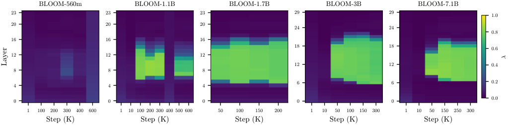
Refer to caption — Figure 41: BLOOM training dynamics: sampled $\lambda$ per layer (vertical) across intermediate checkpoints (horizontal). Columns at non-equal step intervals reflect the available BLOOM checkpoints after excluding duplicate uploads.

B.9 Instruction Tuning Effects

Figures 49–59 replicate the 3-panel layout of §B.1 for the instruction-tuned variants we evaluate: BLOOMZ (560m–7.1B), Qwen3-Instruct (0.6B–14B), and SmolLM3-3B-Instruct. The base counterparts are in Figures 5–25 for direct comparison.

Effect sizes vary sharply by family. In BLOOMZ the largest shift is at the smallest scale: BLOOMZ-560m moves from a weak mid-layer peak ( $\lambda=0.21$ in base) to a full sharing plateau ( $\lambda=0.84$ ), with ILO rising in parallel ( $0.25\to 0.37$ ). The remaining BLOOM sizes already exhibit sharing in the base model and gain only modest peak- $\lambda$ increments ( $+0.02$ to $+0.07$ ); peak ILO rises more substantially across all BLOOM sizes ( $+0.09$ to $+0.15$ ). Qwen3-Instruct and SmolLM3-3B-Instruct show negligible changes in either metric (peak- $\lambda$ within $\pm 0.03$ , peak-ILO within $\pm 0.03$ ), consistent with their base models already operating near the upper end of the sharing range. CKA and ANC profiles change only marginally across all families.

Figure 49: BLOOMZ-560m. Panels as in Fig. 5.

Figure 50: BLOOMZ-1.1B. Panels as in Fig. 5.

Figure 51: BLOOMZ-1.7B. Panels as in Fig. 5.

Figure 52: BLOOMZ-3B. Panels as in Fig. 5.

Figure 53: BLOOMZ-7.1B. Panels as in Fig. 5.

Figure 54: Qwen3-0.6B-Instruct. Panels as in Fig. 5.

Figure 55: Qwen3-1.7B-Instruct. Panels as in Fig. 5.

Figure 56: Qwen3-4B-Instruct. Panels as in Fig. 5.

Figure 57: Qwen3-8B-Instruct. Panels as in Fig. 5.

Figure 58: Qwen3-14B-Instruct. Panels as in Fig. 5.

Figure 59: SmolLM3-3B-Instruct. Panels as in Fig. 5.

B.10 Finetuning Effects

We re-applied the four sharing metrics to each finetuned model at the best learning rate from Appendix A.6, with peak layer fixed at the base-model peak. Table 16 summarizes the resulting shifts and Tables 17–21 report the per-task breakdown. The analysis covers all 21 models $\times$ 5 tasks = 105 (model, task) pairs.

	$\lambda$	ILO	CKA	ANC
Median $\|\Delta\|$	0.003	0.021	0.009	0.010
P90 $\|\Delta\|$	0.035	0.119	0.171	0.113
# pairs $\|\Delta\|\!>\!0.05$	8	31	24	19
# pairs $\|\Delta\|\!>\!0.10$	4	14	16	12

Table 16: Distribution of peak-metric shifts after cross-lingual finetuning across 105 (model, task) pairs.

BLOOM
Model	$\Delta\lambda$	$\Delta$ ILO	$\Delta$ CKA	$\Delta$ ANC
BLOOM-560M	+0.068	+0.022	+0.002	+0.003
BLOOM-1b1	+0.023	+0.035	+0.001	+0.007
BLOOM-1b7	+0.016	+0.030	$-$ 0.000	+0.006
BLOOM-3B	+0.025	+0.049	+0.001	+0.016
BLOOM-7b1	+0.016	+0.042	$-$ 0.002	+0.004
OPT
OPT-125M	+0.000	+0.000	$-$ 0.000	$-$ 0.002
OPT-350M	$-$ 0.001	+0.000	+0.005	$-$ 0.003
OPT-1.3B	+0.004	+0.016	+0.009	$-$ 0.009
OPT-2.7B	$-$ 0.001	+0.006	+0.037	$-$ 0.020
OPT-6.7B	+0.001	+0.011	+0.014	$-$ 0.008
XGLM
XGLM-564M	+0.000	$-$ 0.003	$-$ 0.001	+0.002
XGLM-1.7B	+0.000	+0.124	$-$ 0.249	+0.113
XGLM-2.9B	+0.001	+0.127	$-$ 0.067	+0.002
XGLM-4.5B	+0.000	$-$ 0.115	$-$ 0.033	$-$ 0.162
XGLM-7.5B	$-$ 0.002	+0.288	$-$ 0.199	$-$ 0.007
Qwen3
Qwen3-0.6B	+0.006	+0.102	+0.000	+0.011
Qwen3-1.7B	$-$ 0.008	+0.075	+0.003	+0.016
Qwen3-4B	+0.001	+0.011	$-$ 0.015	$-$ 0.004
Qwen3-8B	+0.001	+0.012	$-$ 0.042	+0.001
Qwen3-14B	$-$ 0.001	+0.009	$-$ 0.000	$-$ 0.006
SmolLM3
SmolLM3-3B	+0.003	+0.013	$-$ 0.005	+0.001

Table 17: Peak-metric shifts after finetuning on Belebele. Positive values indicate the finetuned model’s peak metric exceeds the base model’s; the peak layer is read independently per metric on the base model.

BLOOM
Model	$\Delta\lambda$	$\Delta$ ILO	$\Delta$ CKA	$\Delta$ ANC
BLOOM-560M	+0.073	$-$ 0.021	$-$ 0.343	$-$ 0.034
BLOOM-1b1	+0.003	+0.003	$-$ 0.000	+0.001
BLOOM-1b7	+0.001	+0.001	$-$ 0.001	+0.006
BLOOM-3B	+0.006	+0.005	+0.001	$-$ 0.000
BLOOM-7b1	+0.006	+0.010	$-$ 0.009	+0.015
OPT
OPT-125M	$-$ 0.001	$-$ 0.001	$-$ 0.001	$-$ 0.003
OPT-350M	$-$ 0.000	$-$ 0.000	+0.001	+0.006
OPT-1.3B	$-$ 0.001	$-$ 0.000	+0.013	$-$ 0.008
OPT-2.7B	$-$ 0.002	$-$ 0.005	+0.018	$-$ 0.003
OPT-6.7B	$-$ 0.002	$-$ 0.005	+0.008	+0.002
XGLM
XGLM-564M	$-$ 0.001	$-$ 0.012	+0.001	$-$ 0.042
XGLM-1.7B	+0.000	+0.058	$-$ 0.022	+0.134
XGLM-2.9B	$-$ 0.001	+0.042	$-$ 0.214	$-$ 0.023
XGLM-4.5B	$-$ 0.000	+0.048	$-$ 0.009	$-$ 0.041
XGLM-7.5B	$-$ 0.001	+0.208	$-$ 0.284	$-$ 0.016
Qwen3
Qwen3-0.6B	+0.002	+0.009	+0.000	+0.008
Qwen3-1.7B	+0.000	+0.010	+0.000	+0.003
Qwen3-4B	$-$ 0.001	+0.000	$-$ 0.001	+0.000
Qwen3-8B	$-$ 0.002	+0.004	+0.027	+0.005
Qwen3-14B	$-$ 0.000	$-$ 0.004	+0.000	$-$ 0.002
SmolLM3
SmolLM3-3B	$-$ 0.000	$-$ 0.001	+0.001	$-$ 0.000

Table 18: Peak-metric shifts after finetuning on SIB-200. Columns and conventions as in Table 17.

BLOOM
Model	$\Delta\lambda$	$\Delta$ ILO	$\Delta$ CKA	$\Delta$ ANC
BLOOM-560M	+0.051	+0.072	$-$ 0.003	+0.013
BLOOM-1b1	$-$ 0.308	+0.106	$-$ 0.015	+0.033
BLOOM-1b7	+0.029	+0.094	$-$ 0.023	$-$ 0.021
BLOOM-3B	+0.033	+0.066	$-$ 0.004	$-$ 0.005
BLOOM-7b1	+0.013	+0.074	$-$ 0.022	$-$ 0.014
OPT
OPT-125M	+0.001	$-$ 0.000	$-$ 0.001	+0.004
OPT-350M	$-$ 0.008	+0.000	+0.006	+0.005
OPT-1.3B	+0.006	+0.004	$-$ 0.061	$-$ 0.091
OPT-2.7B	+0.022	$-$ 0.012	$-$ 0.058	$-$ 0.143
OPT-6.7B	+0.002	$-$ 0.007	$-$ 0.001	$-$ 0.052
XGLM
XGLM-564M	$-$ 0.000	+0.077	$-$ 0.088	$-$ 0.173
XGLM-1.7B	+0.008	+0.223	$-$ 0.171	+0.071
XGLM-2.9B	+0.009	+0.175	$-$ 0.093	$-$ 0.008
XGLM-4.5B	+0.008	+0.229	$-$ 0.056	+0.080
XGLM-7.5B	$-$ 0.001	+0.293	$-$ 0.206	+0.003
Qwen3
Qwen3-0.6B	+0.012	+0.119	+0.000	+0.012
Qwen3-1.7B	+0.008	+0.074	+0.001	+0.028
Qwen3-4B	+0.004	+0.072	$-$ 0.117	$-$ 0.003
Qwen3-8B	$-$ 0.003	+0.064	$-$ 0.036	$-$ 0.157
Qwen3-14B	$-$ 0.006	+0.019	$-$ 0.532	$-$ 0.437
SmolLM3
SmolLM3-3B	+0.003	+0.023	$-$ 0.021	$-$ 0.004

Table 19: Peak-metric shifts after finetuning on XNLI. Columns and conventions as in Table 17.

BLOOM
Model	$\Delta\lambda$	$\Delta$ ILO	$\Delta$ CKA	$\Delta$ ANC
BLOOM-560M	+0.272	+0.042	+0.001	+0.014
BLOOM-1b1	+0.048	+0.055	$-$ 0.041	$-$ 0.004
BLOOM-1b7	+0.051	+0.053	$-$ 0.015	+0.012
BLOOM-3B	+0.047	+0.041	$-$ 0.018	+0.001
BLOOM-7b1	+0.013	+0.025	$-$ 0.006	$-$ 0.008
OPT
OPT-125M	$-$ 0.002	+0.000	$-$ 0.003	$-$ 0.044
OPT-350M	$-$ 0.000	+0.000	$-$ 0.001	$-$ 0.014
OPT-1.3B	$-$ 0.000	$-$ 0.000	+0.010	$-$ 0.024
OPT-2.7B	$-$ 0.001	$-$ 0.008	+0.027	$-$ 0.026
OPT-6.7B	+0.006	$-$ 0.014	+0.007	$-$ 0.026
XGLM
XGLM-564M	$-$ 0.003	+0.002	$-$ 0.023	$-$ 0.208
XGLM-1.7B	$-$ 0.001	+0.097	$-$ 0.098	+0.155
XGLM-2.9B	$-$ 0.002	+0.070	$-$ 0.168	$-$ 0.026
XGLM-4.5B	+0.006	+0.084	$-$ 0.053	+0.056
XGLM-7.5B	$-$ 0.001	+0.236	$-$ 0.192	$-$ 0.021
Qwen3
Qwen3-0.6B	$-$ 0.003	+0.064	$-$ 0.001	+0.001
Qwen3-1.7B	$-$ 0.006	+0.066	+0.001	$-$ 0.007
Qwen3-4B	$-$ 0.007	+0.009	$-$ 0.115	$-$ 0.005
Qwen3-8B	$-$ 0.002	+0.013	$-$ 0.026	$-$ 0.028
Qwen3-14B	+0.001	+0.009	$-$ 0.009	+0.009
SmolLM3
SmolLM3-3B	$-$ 0.003	$-$ 0.011	$-$ 0.009	$-$ 0.010

Table 20: Peak-metric shifts after finetuning on XCSR. Columns and conventions as in Table 17.

BLOOM
Model	$\Delta\lambda$	$\Delta$ ILO	$\Delta$ CKA	$\Delta$ ANC
BLOOM-560M	$-$ 0.139	+0.021	$-$ 0.027	$-$ 0.004
BLOOM-1b1	$-$ 0.163	$-$ 0.003	$-$ 0.001	$-$ 0.007
BLOOM-1b7	$-$ 0.001	$-$ 0.012	$-$ 0.002	$-$ 0.014
BLOOM-3B	+0.014	$-$ 0.025	+0.001	$-$ 0.019
BLOOM-7b1	+0.003	$-$ 0.015	$-$ 0.001	$-$ 0.011
OPT
OPT-125M	+0.002	+0.001	$-$ 0.000	$-$ 0.002
OPT-350M	$-$ 0.006	+0.001	$-$ 0.021	$-$ 0.020
OPT-1.3B	+0.020	$-$ 0.020	$-$ 0.128	$-$ 0.080
OPT-2.7B	+0.014	$-$ 0.044	$-$ 0.262	$-$ 0.125
OPT-6.7B	+0.035	$-$ 0.037	$-$ 0.005	$-$ 0.061
XGLM
XGLM-564M	$-$ 0.001	$-$ 0.027	$-$ 0.006	$-$ 0.183
XGLM-1.7B	$-$ 0.000	+0.047	$-$ 0.151	+0.103
XGLM-2.9B	$-$ 0.001	+0.031	$-$ 0.009	$-$ 0.032
XGLM-4.5B	+0.005	+0.031	$-$ 0.049	+0.037
XGLM-7.5B	$-$ 0.002	+0.178	$-$ 0.195	$-$ 0.026
Qwen3
Qwen3-0.6B	$-$ 0.009	$-$ 0.034	$-$ 0.000	+0.004
Qwen3-1.7B	$-$ 0.006	$-$ 0.023	+0.000	$-$ 0.001
Qwen3-4B	+0.000	$-$ 0.002	+0.000	+0.000
Qwen3-8B	+0.001	$-$ 0.017	+0.017	$-$ 0.004
Qwen3-14B	+0.000	$-$ 0.008	+0.001	$-$ 0.004
SmolLM3
SmolLM3-3B	+0.001	$-$ 0.005	$-$ 0.001	$-$ 0.002

Table 21: Peak-metric shifts after finetuning on XQuAD. Columns and conventions as in Table 17.

Appendix C Statistical Analysis

All correlations in this section use Spearman’s $\rho$ between a per-model peak (or mean) sharing metric and transfer scores over the five tasks reported in Appendix B.7 ( $n=21$ base models, 5 families).

C.1 Primary Correlation Analysis

Table 22 reports the headline Spearman $\rho$ between each sharing metric and transfer scores with raw and Benjamini–Hochberg-adjusted $p$ -values across the four-metric family. ILO and ANC are significant under both; $\lambda$ is significant but weak; CKA is not.

Metric	$\rho$	$p_{\text{raw}}$	$p_{\text{BH}}$
ILO	$0.901$	${<}.001$	${<}.001$
ANC (mean)	$0.839$	${<}.001$	${<}.001$
$\lambda$	$0.525$	$.015$	$.020$
CKA (mean)	$0.136$	$.556$	$.556$

Table 22: Primary Spearman correlations between sharing metrics and mean cross-lingual transfer (

n=21

base models across 5 families).

p_{\text{BH}}

is the Benjamini–Hochberg-adjusted

p

-value across the four metric tests.

Without OPT.

OPT is our English-only baseline and the only family in our set without explicit multilingual pretraining. Table 23 repeats the analysis on the remaining $n=16$ multilingual models. ILO remains the strongest ( $\rho=0.78$ ); ANC drops ( $\rho=0.64$ ), close to $\lambda$ ( $\rho=0.66$ ); CKA remains non-significant.

Metric	$\rho$	$p_{\text{raw}}$	$p_{\text{BH}}$
ILO	$0.777$	${<}.001$	$.002$
$\lambda$	$0.656$	$.006$	$.011$
ANC (mean)	$0.635$	$.008$	$.011$
CKA (mean)	$0.112$	$.680$	$.680$

Table 23: Primary correlations after excluding OPT (

n=16

multilingual models across 4 families: BLOOM, XGLM, Qwen3, SmolLM3). Removing the English-only contrast reduces every correlation; ILO remains the strongest (

0.78

), with

\lambda

(

0.66

) and ANC (

0.64

) in a second tier.

C.2 Partial Spearman Correlations

Larger models tend to share more and to transfer better, so the headline correlations could in principle reflect model scale rather than sharing. Table 24 reports the partial Spearman $\rho$ holding $\log_{10}$ (parameter count) fixed. ILO and ANC are largely unchanged; $\lambda$ is essentially unchanged; CKA increases modestly but remains weak.

Metric	$\rho$	$\rho_{\text{partial}}$
ILO	$0.901$	$0.845$
ANC (mean)	$0.839$	$0.836$
$\lambda$	$0.525$	$0.504$
CKA (mean)	$0.136$	$0.286$

Table 24: Partial Spearman correlations controlling for

\log_{10}

(parameter count) (

n=21

base models).

\rho

reproduces the raw Spearman correlation;

\rho_{\text{partial}}

is the same correlation after partialling out model size.

C.3 Consistent Layer Aggregation

The results in the main text summarize ILO and $\lambda$ at their peak-sharing layer but CKA and ANC as the mean over layers and language pairs. Because a max-of-layers statistic and a mean-of-layers statistic have different sampling behaviour, differences between metrics could in principle reflect the summary rule rather than the metrics themselves. We therefore compute all transfer correlations under two consistent rules. For every metric we first form a per-layer profile by averaging over languages or language pairs within each layer (exactly how the ILO profile is constructed), and then take either the profile maximum (all-peak) or the profile mean over all layers (all-mean).

Table 25 reports the result. The ranking of metrics is identical under both consistent rules and identical to the mixed convention used in the main text: ILO strongest, ANC a clear second tier, $\lambda$ moderate, CKA null. ILO and ANC are stable to within $0.04$ across rules on every statistic. $\lambda$ is the only metric with a notable aggregation sensitivity: under all-mean its cross-model correlation weakens ( $0.52\to 0.46$ ) and its per-family correlations turn negative in three of four families (OPT $-0.90$ , Qwen3 $-0.50$ , XGLM $-0.70$ ), so its already-fragile within-family behaviour (§C.7) additionally depends on the summary rule. CKA does not improve when given the same peak treatment as ILO ( $\rho=0.12$ ). The comparison in the main text is therefore not an artifact of the mixed summary convention.

Rule	Metric	$\rho$	$p_{\text{BH}}$	$\rho_{\text{partial}}$	$p_{\text{perm}}^{\text{within-fam}}$
all-peak	ILO	$0.901$	${<}.001$	$0.845$	$.014$
	ANC	$0.840$	${<}.001$	$0.846$	$.43$
	$\lambda$	$0.525$	$.020$	$0.504$	$.056$
	CKA	$0.116$	$.618$	$0.332$	$.87$
all-mean	ILO	$0.882$	${<}.001$	$0.804$	$.009$
	ANC	$0.839$	${<}.001$	$0.836$	$.39$
	$\lambda$	$0.458$	$.049$	$0.560$	$.96$
	CKA	$0.136$	$.556$	$0.286$	$.93$

Table 25: Transfer correlations under consistent layer-aggregation rules (

n=21

base models). Every metric is summarized by the same rule: peak of the per-layer profile (all-peak) or mean over all layers (all-mean); profiles average over languages or language pairs within each layer.

p_{\text{BH}}

is Benjamini–Hochberg-adjusted across the four metric tests per rule;

\rho_{\text{partial}}

controls for

\log_{10}

(parameters);

p_{\text{perm}}^{\text{within-fam}}

is the within-family permutation test of §3.5 (

10{,}000

shuffles). ILO is the only metric that survives the within-family permutation under either rule, and the metric ranking is identical under both.

Table 26 reports where each metric peaks. ILO peaks in the middle third of the network in nearly every model (relative depth $0.23$ – $0.65$ ), consistent with the inverted-U profiles of Figure 2. CKA’s peak location is unstable across models: it falls on the embedding layer (layer 0) in the smallest OPT and XGLM models but on the second-to-last layer in Qwen3-4B/8B and SmolLM3. Peak CKA therefore selects qualitatively different computational stages in different models, shared lexical statistics near the embeddings in some and output-adjacent similarity in others, rather than the mid-network stage that peak ILO consistently identifies, which is a further indication that CKA does not track the sharing phenomenon the other metrics measure. For $\lambda$ in XGLM, the reported peak at layer 0 is not meaningful: the profile is near-zero and flat, so no peak exists to locate.

Model	$L$	ILO	$\lambda$	CKA	ANC
BLOOM-560m	23	12	10	12	16
BLOOM-1b1	23	14	11	7	14
BLOOM-1b7	23	15	11	11	17
BLOOM-3b	29	17	18	15	20
BLOOM-7b1	29	17	16	17	21
OPT-125m	11	0	0	0	8
OPT-350m	23	0	0	0	21
OPT-1.3b	23	15	0	3	19
OPT-2.7b	31	19	3	5	25
OPT-6.7b	31	19	3	24	25
XGLM-564M	23	11	0	0	3
XGLM-1.7B	23	11	0	0	15
XGLM-2.9B	47	11	0	6	7
XGLM-4.5B	47	19	0	5	21
XGLM-7.5B	31	17	0	3	3
Qwen3-0.6B	27	15	8	15	10
Qwen3-1.7B	27	15	12	15	10
Qwen3-4B	35	11	15	34	11
Qwen3-8B	35	18	14	34	11
Qwen3-14B	39	24	15	20	14
SmolLM3-3B	35	10	10	34	10

Table 26: Peak-layer locations per metric (peak of the per-layer profile;

L

= number of layers). ILO peaks mid-network in all models. CKA peaks at the embedding layer in the smallest OPT/XGLM models but at the second-to-last layer in Qwen3-4B/8B and SmolLM3, so its peak does not correspond to a comparable computational stage across models.

\lambda

’s layer-0 peaks in XGLM reflect a near-zero flat profile rather than a genuine maximum.

C.4 Per-Language Correlations

The correlations in the main text aggregate each metric and the transfer score to one value per model. To test whether the model-level association merely averages away per-language structure, we repeat the analysis at the (model, language) level: 21 base models $\times$ 9 non-English target languages $=$ 189 points, with per-language transfer defined as the mean over each task’s per-language scores (Appendix B.7).

Per-language metric values use the same profile-peak rule as Appendix C.3. For ILO, we take each language’s own ILO profile peak; ILO counts neighbours from any other language, so this measures how integrated a language is in the shared space. CKA and ANC are pairwise, which permits two constructs: alignment of the target language with English, the finetuning source (vs. English), and the mean over all nine pairs involving the target (all pairs). $\lambda$ is defined jointly over all languages and has no per-language form, so it does not participate in this analysis.

We report the median within-model Spearman $\rho$ (each model contributes one correlation across its nine target languages) with the number of models where it is positive, and a pooled partial Spearman $\rho$ over all 189 points controlling for model-level transfer, computed once more with English-target subword overlap as an additional control, which addresses the possibility that per-language associations are lexical rather than representational. A permutation test in the within-family design of §3.5, applied at the language level ( $10{,}000$ shuffles of per-language transfer within each model, statistic: the model-controlled partial $\rho$ ), confirms the pooled association for every metric variant ( $p<.001$ ), so the table distinguishes the variants by effect size rather than by significance.

Metric	$\tilde{\rho}_{\text{within}}$	$+$	$\rho_{\text{ctrl}}$	$\rho_{\text{ctrl+ov}}$
ILO	$0.68$	20/21	$0.73$	$0.70$
ANC (vs. English)	$0.77$	20/21	$0.69$	$0.67$
ANC (all pairs)	$0.77$	20/21	$0.49$	$0.46$
CKA (vs. English)	$0.47$	18/21	$0.43$	$0.36$
CKA (all pairs)	$0.32$	17/21	$0.18$	$0.11$

Table 27: Per-language metric vs. per-language transfer (21 models

\times

9 target languages

=

189 points).

\tilde{\rho}_{\text{within}}

: median within-model Spearman

\rho

(

n=9

languages per model);

+

: models with a positive within-model correlation;

\rho_{\text{ctrl}}

: pooled partial

\rho

controlling for model-level transfer;

\rho_{\text{ctrl+ov}}

: additionally controlling for English-target subword overlap. All variants pass the within-model permutation test (

p<.001

; see text).

Three observations follow from Table 27. First, the model-level conclusion is not an artifact of aggregation: per-language ILO correlates positively with per-language transfer within 20 of the 21 models (the exception, Qwen3-14B, is a flat $\rho=-0.12$ , $p=.77$ ), with a median within-model $\rho$ of $0.68$ . Second, subword overlap does not account for the association: controlling for English-target overlap changes the ILO and ANC (vs. English) partial correlations by no more than $0.04$ , so the per-language signal is representational rather than lexical, although the overlap channel exists. Third, for the pairwise metrics, what predicts a language’s transfer is its alignment with English, the finetuning source, rather than its average alignment with the other languages: CKA between the target and English tracks transfer ( $\tilde{\rho}_{\text{within}}=0.47$ ), whereas CKA averaged over the target’s other pairs is weaker ( $0.32$ ) and near zero once overlap is controlled ( $0.11$ ), and ANC shows the same ordering under model-level controls ( $0.69$ vs. $0.49$ ). ILO is the exception: its any-language neighbourhood construct predicts transfer without referencing the source language at all.

C.5 Permutation Tests

Table 28 reports permutation $p$ -values from two null distributions. $p_{\text{perm}}^{\text{full}}$ permutes transfer scores freely across all 21 models. $p_{\text{perm}}^{\text{within-fam}}$ permutes only within each family, retaining all between-family contrasts; this asks whether the metric–transfer association exists inside families rather than as a between-family ordering alone. ILO survives both tests (within-family $p=.014$ ); $\lambda$ is borderline under the within-family permutation ( $p=.056$ ) and ANC and CKA fail it outright.

Metric	$\rho$	$p_{\text{naive}}$	$p_{\text{perm}}^{\text{full}}$	$p_{\text{perm}}^{\text{within-fam}}$
ILO	$0.901$	${<}.001$	$.0001$	$.014$
ANC (mean)	$0.839$	${<}.001$	$.0001$	$.405$
$\lambda$	$0.525$	$.015$	$.018$	$.056$
CKA (mean)	$0.136$	$.556$	$.558$	$.931$

Table 28: Permutation tests (

n=21

, four families with

\geq 2

members eligible for within-family permutation). The within-family permutation shuffles transfer scores only within each family, retaining all between-family contrasts; it is the most stringent test of whether the metric–transfer association exists inside a family rather than as a between-family ordering only.

C.6 Per-Task Heterogeneity

Table 29 reports per-task Spearman $\rho$ to test whether the headline average masks task-level differences. ILO is significant on all five tasks ( $\rho\in[0.73,0.88]$ ); ANC is significant on all five, though weakest on SIB-200; $\lambda$ is significant only on Belebele and XQuAD, dropping to non-significant on XNLI, XCSR, and SIB-200; CKA reaches no task.

Metric	Belebele	XNLI	XCSR	SIB-200	XQuAD
ILO	$0.866^{***}$	$0.877^{***}$	$0.836^{***}$	$0.726^{***}$	$0.840^{***}$
ANC (mean)	$0.761^{***}$	$0.812^{***}$	$0.735^{***}$	$0.614^{*\hphantom{}}$	$0.878^{***}$
$\lambda$	$0.668^{*\hphantom{}}$	$0.425^{\hphantom{***}}$	$0.271^{\hphantom{***}}$	$0.148^{\hphantom{***}}$	$0.636^{*\hphantom{}}$
CKA (mean)	$0.265^{\hphantom{***}}$	$0.068^{\hphantom{***}}$	$0.073^{\hphantom{***}}$	$-0.231^{\hphantom{***}}$	$0.251^{\hphantom{***}}$

Table 29: Per-task Spearman

\rho

between each sharing metric and per-task cross-lingual transfer (

n=21

). Significance under BH-FDR over the 20-test pool:

{}^{*}:p<.05

{}^{**}:p<.01

{}^{***}:p<.001

. ILO is the only metric significant across all five tasks;

\lambda

drops to non-significant on XNLI, XCSR, and SIB-200.

C.7 Within-Family Breakdown

Per-family Spearman $\rho$ uses $n=5$ models per family and therefore has low individual-test power, but the sign and direction of the four family-level correlations is informative in itself. Table 30 reports per-family $\rho$ . ILO is positive in three of four families and flat on XGLM ( $-0.10$ ); with $n=5$ per family these individual coefficients are individually uninformative, which is why our within-family claims rest on the within-family permutation test ( $p=.014$ ), which ILO alone survives. $\lambda$ flips sign on OPT ( $-0.90$ ): more sharing predicts less transfer inside the OPT family. ANC flips sign on XGLM ( $-0.70$ ). CKA is non-positive in 3 of 4 families, yet its cross-model $\rho$ from Table 22 is positive: the weak positive cross-model CKA–transfer ordering is driven by between-family means, not by any within-family relationship.

Metric	BLOOM	OPT	Qwen3	XGLM
ILO	$+0.90$	$+1.00$	$+1.00$	$-0.10$
ANC (mean)	$+0.90$	$+1.00$	$+0.70$	$-0.70$
$\lambda$	$+0.60$	$-0.90$	$+0.70$	$+0.30$
CKA (mean)	$0.00$	$-0.40$	$-0.50$	$-0.10$

Table 30: Within-family Spearman

\rho

per family (

n=5

per family). SmolLM3 is a singleton and is omitted. ILO is positive in three of four families and flat on XGLM (

-0.10

). ANC shows a sign reversal on XGLM (

-0.70

);

\lambda

flips sign on OPT (

-0.90

); CKA is non-positive in 3 of 4 families.

A Systematic Comparison of Multilingual Interpretability Methods Reveals Anisotropy-Driven Failures