On the spectrality of the non-homogeneous golden-mean self-similar measure
Abstract.
We investigate the spectral properties of a class of inhomogeneous self-similar measures, which does not admit a non-trivial infinite convolution structure. A central example is the golden-mean self-similar measure , for which the existence of an exponential orthonormal basis in the associated -space has remained a long-standing open problem. The usual approach for homogeneous self-similar measures does not apply here, new methods are required. We establish several basic properties of the measure and then carry out a detailed numerical study of the zero set of its Fourier transform. Using a scanning and refinement algorithm that combines uniform grid sampling, quadratic interpolation, and golden-section search, we examine a wide range and find no real zeros of , which provides concrete evidence that is very likely non-spectral, suggesting that inhomogeneity may serve as a natural obstruction to the existence of exponential orthonormal bases. To the best of our knowledge, our paper is the first attempt to study the spectrality of such measures through a combined analytic and numerical framework.
Key words and phrases:
golden-mean self-similar measure, spectrality, zero set2020 Mathematics Subject Classification
Primary 42B10; Secondary 28A801. Introduction
A compactly supported Borel probability measure on is called spectral if there exists a countable set such that
forms an orthonormal basis for . The set is then called a spectrum of .
Research on spectral measures originated with Fuglede [8], who formulated his celebrated conjecture: the normalized Lebesgue measure on a set of positive finite Lebesgue measure is a spectral measure (also call a spectral set) if and only if tiles by translations. Both directions of the conjecture are false for ; see [14] and the references therein. For , however, both directions remain open. This problem has motivated extensive research into the properties that make a set or a measure spectral.
In 1998, Jorgensen and Pedersen [11] constructed the first example of a non-atomic singular spectral measure, i.e., the standard middle-fourth Cantor measure . Following this discovery, the spectrality of fractal measures including self-similar measures, self-affine measures, and Moran measures has been extensively explored; see [1, 5, 6, 7, 12] and the references therein. A crucial common feature of all these known spectral measures is that they can be expressed as an infinite convolution of finitely supported discrete measures. This convolution structure is what makes it possible to construct explicit spectra, and it remains the foundation of the known sufficient conditions for spectrality.
However, not all fractal measures admit such an infinite convolution structure. In this paper, we consider non-homogeneous self-similar measures. Let and . Let and be an iterated function system on . By Hutchinson’s theorem [10], there exists a unique Borel probability measure with non-empty compact support satisfying that
| (1.1) |
for any Borel set and is the unique compact set satisfying
| (1.2) |
The probability measure satisfying (1.1) is called a self-similar measure and is called a self-similar set or attractor. When , the measure is the classical Bernoulli convolution. In particular, taking and , is exactly the aforementioned .
For the classical Bernoulli convolution, it is known that is a spectral measure if and only if for some and [3, 6]. For the case , its spectrality remains largely mysterious. The reason why the non-homogeneous case is much more difficult than the homogeneous one is that while is an infinite convolution of Bernoulli measures, is not. The convolution structure is crucial to all the previous results. A long-standing folklore open problem in the community of fractal spectral measure theory is the following:
Question 1.1.
For , when is a spectral measure?
We write
| (1.2) |
for the similarity dimension of the measure . To the best of our knowledge, apart from the classical setting, there are virtually no methods or results concerning the spectrality of in the absolutely continuous case. In this paper, we focus primarily on the singular case (a well-known sufficient condition for the measure to be singular is ). However, even in this singular case, the problem remains notoriously difficult. Therefore, we restrict our attention to the condition (which is stronger than ), under which the singularity of the measure is guaranteed and the analysis becomes relatively tractable.
In the case , He, Kang, Tang and the second author [9] obtained a necessary condition for the spectrality of . Specifically, they proved that if there exists a spectrum of such that its Beurling dimension is equal to the Hausdorff dimension of (a natural condition that holds in the classical Bernoulli convolution case), then must satisfy , where is determined by . In this setting, coincides with defined in (1.2).
On the other hand, up to now, every known singular continuous spectral measure has no Fourier decay. For , it has Fourier decay whenever the two contraction ratios are not logarithmically commensurable, i.e., [13]. Motivated by this fact, we shall restrict our attention to the logarithmically commensurable case.
In this paper, we focus on the simplest case of the general framework described above, namely the golden-mean self-similar measure, which we denote by . It is defined by choosing the contraction ratios and , where is determined by
Equivalently, , where is the golden ratio; this gives rise to the name “golden-mean” self-similar measure.
There is no general result on Fourier decay for non-homogeneous self-similar measures with logarithmically commensurable contraction ratios. However, for the golden-mean measure considered in this paper, we can prove that it has no Fourier decay (see Proposition 3.5 in Section 3).
It is well known that if is a spectral measure with spectrum , then the orthogonality of implies that for all distinct , where
is the Fourier transform of . Since is non-atomic, is infinite-dimensional; consequently, any spectrum must be countably infinite, and must vanish on the infinite difference set . Thus, understanding the zero set of is a natural first step toward determining the spectrality of . In particular, if has no real zeros, or has at most finitely many real zeros, then cannot admit an infinite orthogonal system of exponentials, and hence cannot be spectral.
In this paper, we first set up some basic properties of the gold-mean self-similar measure . Then we develop a scanning and refinement algorithm that combines uniform grid sampling, complex quadratic interpolation, and golden-section search to locate potential zeros of the auxiliary Riccati function with high precision. The algorithm proceeds in two phases: a coarse scan over a uniform grid to detect local minima of , followed by a refined search using quadratic interpolation and golden-section search to pinpoint candidate zeros. Using this algorithm, we examine the interval and find no real zeros of . Together with the theoretical analysis on the interval (see Proposition 3.3), this provides concrete numerical evidence that is very likely non-spectral.
Although the interval derived by the rigorous analysis may seem small, this is not an essential limitation. A larger interval could be obtained by more refined estimates, but the required technical effort would be considerable and, in our view, disproportionate to the additional benefit, especially since the numerical scan already rules out zeros with high precision over the much larger interval .
2. Elementary properties of the golden-mean self-similar measure
In this section, we will set up some basic properties of the gold-mean self-similar measure . Some of these may be known in more general case, but we give simpler proofs here. For simplicity, we write and . Let . For , let be the set of words of length and let be the set of infinite words.
2.1. Self-similar set and binary expansions
We now give a convenient description of the self-similar set associated to the gold-mean self-similar measure in terms of binary expansions.
Proposition 2.1.
Let be the attractor of the golden-mean iterated function system . Then
Equivalently, consists of the points in that admit a binary expansion with no two consecutive ’s.
Proof.
Let
Equip with the standard product topology and it is well-known that is compact. It is easy to see that the set is closed and thus is compact. Note that the map
is continuous and so is compact. Moreover, is nonempty because the zero sequence belongs to . Then, by (1.2) we only need to show that satisfies
Take and write with all . If , then
Since contains no consecutive ’s, it follows that and . If , then the definition of forces . Hence
The sequence again contains no consecutive ’s.Then and . In either case lies in , proving .
To prove the other direction, if , then for some . Write with all . Then
where and for . The sequence contains no consecutive ’s from and then . If . Then for some . Write with all . Then
Thus . ∎
2.2. Singular continuity of
Proposition 2.2.
The golden-mean self-similar measure is non-atomic and singular with respect to Lebesgue measure.
Proof.
We first prove that is non-atomic. Let and , where is defined by . Then .
For a word with for , write and . By Proposition 2.1, for any with all , the no consecutive ones constraint gives
i.e., . Hence , and
which implies that . Therefore, by (1.1)
where .
For any , there exists an with all such that for every . Therefore
so . Thus has no atoms.
It remains to show , where denotes the Lebesgue measure. Let . For and each with all , denote . Its length is , where and .
Since , it follows that
where denotes the length of . Thus by letting . Since is supported on , it follows that . The proof is complete. ∎
2.3. Not an infinite Bernoulli convolution
Theorem 2.3.
The golden-mean self-similar measure cannot be represented as an infinite convolution of Bernoulli measures.
To prove it, we need some preliminaries. We first recall the definition of an infinite convolution of Bernoulli measures.
Definition 2.4.
Let be a sequence of positive real numbers satisfying , and let be a sequence with for all . We say that
| (2.1) |
is an infinite convolution of Bernoulli measures, where the convergence is in weak sense.
It is easy to see that the support of is the following set
Proposition 2.5.
Let be an infinite convolution of Bernoulli measures defined in 2.1. Then is centrally symmetric with respect to , i.e., if , then .
Proof.
Let with . Then
since . ∎
Lemma 2.6.
The attractor of the golden-mean iterated function system is not centrally symmetric.
Proof.
We first note that and by Proposition 2.1. If is centrally symmetric, then its center would necessarily be the midpoint of its smallest and largest points. Thus the only possible center would be
Note that with . Then . Consider . It is easy to see that
whose binary expansion contains two consecutive ’s. Hence .
Thus is not symmetric with respect to , and consequently it is not centrally symmetric. ∎
Proof of Theorem 2.3.
Suppose, to the contrary, that,
where , and .
The support of the convolution on the right-hand side is
By Proposition 2.5, is centrally symmetric. Consequently, any translate of is also centrally symmetric.
On the other hand, the support of the golden-mean self-similar measure is the attractor , and Lemma 2.6 shows that is not centrally symmetric. This is a contradiction.
Hence, we complete the proof. ∎
Remark 2.7.
3. The Fourier transform and Riccati equation
Write and set . From (1.1), we obtain for any ,
| (3.1) |
By the definition of the Fourier transform of , .
Define auxiliary measures , and their Fourier transforms . Since , we have
| (3.2) | ||||
Using (3.1) and (3.2), we compute
Together with (3.2) again, this yields the matrix recursion
| (3.3) |
where
Iterating (3.3) times gives
By the continuity of the Fourier transform of a measure, taking yields the convergent representation
| (3.4) |
Proposition 3.1.
For every , . Consequently, if , then . In particular, every real zero of satisfies
| (3.5) |
Proof.
Assume, for a contradiction, that there exists with
i.e., . Since for all , it follows that is invertible. Applying to the left in (3.3) yields
Thus, by induction,
Since is a probability measure, is uniformly continuous on . Letting we obtain , contradicting . Hence for every .
The following proposition is well-known and easy to prove.
Proposition 3.2.
If is orthogonal in , then . Thus implies and is non-spectral.
Proposition 3.3.
does not have a zero in the interval .
Proof.
Since is a positive measure, we have . Hence it suffices to prove that has no zero in . Define
We will show .
First, for , since , we have for -a.e. . Therefore
Thus , and so .
Now let . By (1.1), the intervals and both have -measure . Moreover, for -a.e. , we have , hence
and therefore . Consequently,
| (3.7) |
Using , the integrand in (3.7) equals
For , we have
so the sine factor is positive, and also . Therefore the integrand in (3.7) is strictly positive on , and thus
It follows that , and hence .
At , we have the sharper lower bound
Now define
We have just shown that
Moreover, by the dominated convergence theorem,
where the last equality uses .
Then, for any , the mean value theorem gives some such that
Thus
Taking , we obtain , so . Consequently,
Hence, we complete the proof. ∎
Now define the Riccati function
which is well-defined whenever . From (3.1), whenever , we have
| (3.8) |
with . Iterating this relation formally yields the infinite-product representation
| (3.9) |
provided that all factors are well-defined and the product converges. If the product converges, then exactly when
As an immediate consequence of (3.5), we state the following reformulation.
Remark 3.4.
If for some , then is well-defined and satisfies
and consequently
Thus, a real zero at forces to have modulus exactly and argument exactly . This is a strong two-parameter restriction at each dyadic level. For to have many real zeros, these conditions must hold coherently across all dyadic levels, which is highly restrictive.
At the end of this section. We prove the following:
Proposition 3.5.
The golden-mean self-similar measure has no Fourier decay. More precisely,
so that .
Proof.
Recall that , and the Fourier transform satisfies
| (3.10) |
Set . For , since , we have
The characteristic equation of the above recurrence relation is
whose roots are and . By Theorem 7.2.2 in [2], there exist constants such that
Since , exists.
Using the initial conditions and , we solve for :
Thus is equivalent to
| (3.11) |
We now rule out this possibility. By the proof of Proposition 3.3, for all , we have
In particular, and .
4. Numerical validation of the zero-free property
We describe the computational procedures used to probe the zeroes of the Fourier transform of the golden mean self-similar measure, and report the main numerical observations.
Calculation of the Riccati function
The Fourier transform of the golden-mean self-similar measure is shown by numerical experiments oscillating wildly with a trend toward zero when is large, see Figure 1 (though not strictly approaching zero as is shown in Proposition 3.5). A direct zero hunting of for large is then problematic (due to the risk of shallow valleys of near zero). To find zeros of more accurately, it is therefore more reliable to work with the Riccati function
| (4.1) |
which satisfies the continued-fraction recursion (3.8). Crucially, this recursion automatically renormalizes the value at each scale, keeping mostly within a bounded, moderate range (in fact mostly within as is observed in our numerical scans).

The infinite product representation (see (3.9)), together with the nonzeroness of near implies that the smallest zeroes of and are equivalent. Thus, detecting zeros of is sufficient for finding zeros for . The computation of is done by first truncating the infinite product to get an approximation to and then using (4.1).
4.1. Algorithm for zero detection
Our strategy for locating real zeros of consists of three stages:
- (1)
Coarse uniform scan. On any given interval , we take a uniform step size (typically ) and compute and at each grid point . The step size is chosen to be well below the oscillation period of the exponential factor , (the oscillation period is also well observed from numerical observations below) thereby avoiding aliasing and ensuring that all local minima of are related to local minimums of these sample points.
- (2)
Complex quadratic interpolation and fast valley screening. For every grid point that satisfies
we form the three-point complex quadratic interpolant through the points . Since is analytic on the real axis, the interpolation error is controlled by the third derivative of and is of order in the interval .
To decide whether this valley may contain a zero, we perform a fast golden-section search on with only iterations (plus an early exit if the estimated minimum falls below a given threshold ). This gives an estimated minimum value
If , the valley is flagged as a candidate for further refinement.
- (3)
High-precision refinement on the original function. For each flagged candidate, we apply a full golden-section minimization to the original function on the same interval , iterating until the interval width is below . This yields the refined location and the true minimum value . If is below a very small threshold (e.g., ), we consider it a strong numerical indication of a real zero; otherwise it is recorded as a shallow minimum.
The algorithm is implemented in Python using double-precision floating-point arithmetic, with the infinite product evaluated at depth (which gives an error below machine precision, at least for , as shown in the error analysis below). The code is available upon request.
4.2. Error analysis and reliability of zero detection
We now justify that the above scanning procedure is capable of detecting every real zero in a given interval (we take in the following study) that may exist in the scanned interval, provided the step size and threshold are chosen appropriately. First we show the evaluation of at any given is accurate enough for our purpose.
4.2.1. Error analysis for at given
The numerical evaluation of the Riccati function is based on the finite truncation of the infinite product (3.4). In the program we iterate levels and set the innermost vector to . We choose . We now provide a error analysis, separating the truncation error (due to finite ) from the propagation of floating-point round-off errors.
Truncation error. Let be the matrix
and define the product
The self-similarity of the Fourier transform implies the exact vector identity
Consequently, the true Riccati function is
where and .
The numerical approximation amounts to replaces and by , i.e.,
Now the truncation error is easily calculated as
Since , we have
Moreover, is a Fourier transform of a probability measure, hence for all real , so . Therefore
We note that , and the observed value of is always larger than hence can be replaced by without affecting the error estimates. However, for , . Even if is as small as , the truncation error is bounded by
which is already below double-precision machine epsilon. From the graph 1, it is clear that most of lies above hence we are relatively safe for and in all the scanned are above . Hence the truncation error is negligible in IEEE double precision.
Round-off error propagation. Note the norm of the matrix
then rounding error will not amplify during matrix multiplication. Hence the total error for is estimated to be around times machine epsilon, which is around . Hence is well below the observed minimum of . Now noting the error for is bounded by
since the obeserved minimum of for is around , this value will be around which is negeligible for .
In practice, the main source of uncertainty is not the pointwise evaluation error, but the finite sampling step used in the coarse scans. That issue is addressed below:
4.2.2. Error analysis for finite sampling step
Let be three consecutive grid points with , and let be the unique quadratic polynomial interpolating at these points. The standard interpolation error formula for a complex-analytic function on the real axis gives (for real and imaginary parts, respectively, note might differ)
whenever exists. Hence
where . Taking maximum for the right hand side, we then obtain
Then, if is a zero of ,
Thus, for a fixed tolerance , as long as step size , the above fast valley screening method will capture any potential zeroes that lie within the interval , if we don’t take into account of the computation errors (which by the above analysis is negligible). The constant itself is bounded by certain weighted average modulus of in a neighborhood of of the complex plane (by the Cauchy integral formula). In our numerical experiments, the bound is found to be stable and mostly ; With and , the required inequality for is then satisfied, and we will use these values in our experiment.
Given the above error estimates, the combination of a uniform grid with step , complex quadratic interpolation, and fast golden-section screening is able to capture all local minima of that have depth below when the bounds (, etc.) in the error analysis are stable. The procedure is then complete in the sense that no zero can escape detection. The final refinement on the original function then provides an accurate value of at the minimum, allowing us to decide whether the minimum is consistent with a true zero or merely a shallow valley.
4.3. Main numerical results
As the interval is already covered in thereotical analysis, we applied the algorithm to the interval with step size and screening threshold .
Observed minima of .
No point with was found. The smallest values of encountered in the entire scan are of order . Table 1 lists the ten deepest minima detected.
| 6580077.19160276 | ||
| 5065070.60771886 | ||
| 9084534.95396908 | ||
| 8643446.91961220 | ||
| 1810801.19998039 | ||
| 2717521.23238440 | ||
| 4306582.88129792 | ||
| 883528.97039339 | ||
| 6521201.19741959 | ||
| 4019830.95206717 |
Distribution of .
Figure 2 and Figure 3 display the graph of over two representative subinterval (e.g., around and , one coarse and one fine), showing the typical oscillatory behaviour with period and aggregation of values in the interval. Over the whole scanned range, the oscillatory profile and value aggregations look similar and the minimum value never drops below . Notice the red stars indicate the local minimum points that pass the fast valley screening.
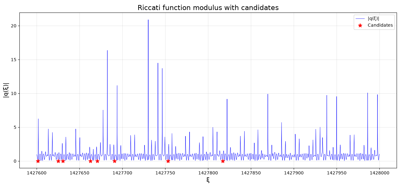
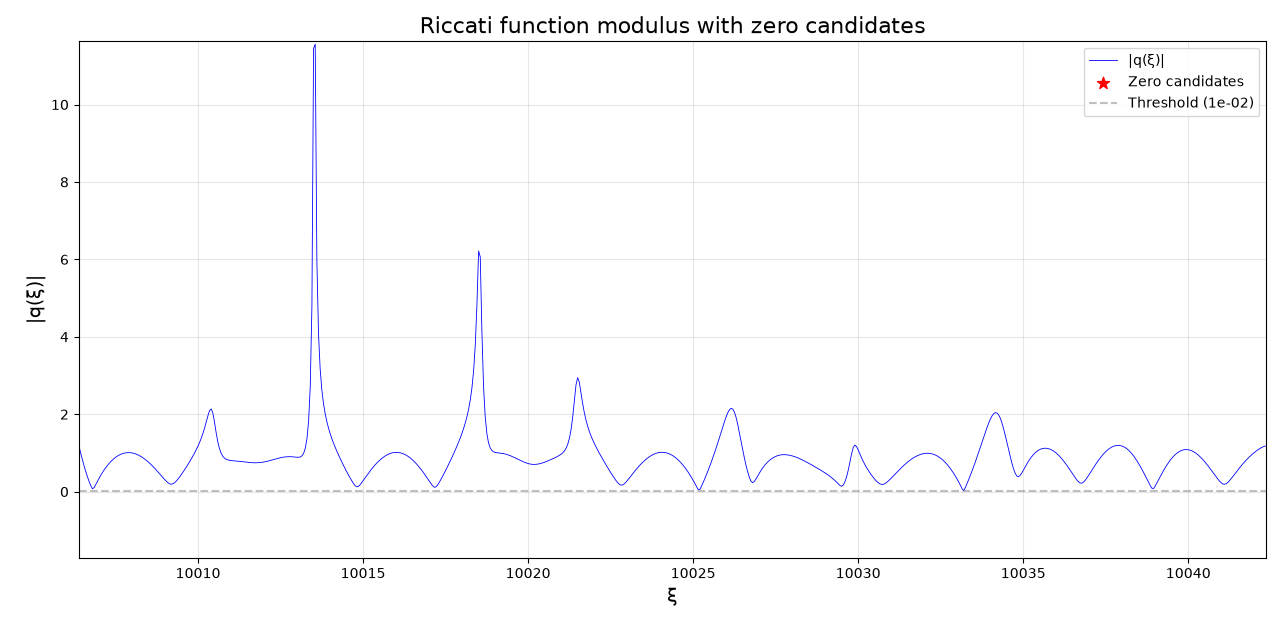
Figure 4 shows the trajectory of on the complex plane with around . Notice the period 2 oscillatory behavior.

The absence of any real zero of (and hence of ) in the scanned range, strongly indicates that has no real zeros at all.
Remark. The present work is numerical and does not constitute a formal proof. A rigorous verification would require a computer-assisted proof, which is left for future investigation. Nevertheless, consistency of our results across multiple independent checks (grid refinements, different thresholds, and comparison with direct computation through the Riccati equation) and above error analysis lends strong support to the conclusion that has no real zeros.
Acknowledgements
The authors would like to thank Professors Xing-Gang He and Xin-Rong Dai for drawing our attention to these problems. The second author would like to thank Professors Meng Wu and Yuan-Yang Chang for helpful discussions on the Fourier decay of self-similar measures; thank Professor Guo-Tai Deng for helpful discussion on the convolution structure of non-homogeneous self-similar measure. The authors were supported by the National Natural Science Foundation of China under Grants 12301131, 12271534 and 12301105.
References
- [1] L. X. An, X. Y. Fu, C. K. Lai, On spectral Cantor-Moran measures and a variant of Bourgain’s sum of sine problem, Adv. Math. 349 (2019), 84–124.
- [2] R. Brualdi, Introductory Combinatorics, 4th ed., Pearson/Prentice Hall, Upper Saddle River, 2004.
- [3] X.-R. Dai, When does a Bernoulli convolution admit a spectrum?, Adv. Math. 231 (2012), 1681–1693.
- [4] G.-T. Deng, Private communication.
- [5] Q.-R. Deng, J. B. Chen, Uniformlity of spectral self-affine measures, Adv. Math. 380 (2021), 107568.
- [6] D. Dutkay, J. Haussermann, C.-K. Lai, Hadamard triples generate self-affine spectral measures, Trans. Amer. Math. Soc. 371 (2019), 1439-1481.
- [7] D. Dutkay, C.-K. Lai, Uniformly of measures with Fourier frames, Adv. Math. 252 (2014), 684–707.
- [8] B. Fuglede, Commuting self-adjoint partial differential operators and a group theoretic problem, J. Funct. Anal. 16 (1974), 101–121.
- [9] X. G. He, Q. C. Kang, M. W. Tang, Z. Y. Wu, Beurling dimension and self-similar measures, J. Funct. Anal. 274 (2018), 2245–2264.
- [10] J. Hutchinson, Fractals and self-similarity, Indiana Univ. Math. J., 30 (1981), 713–747.
- [11] P. Jorgensen, S. Pedersen, Dense analytic subspaces in fractal -spaces, J. Anal. Math. 75 (1998), 185–228.
- [12] I. Łaba, Y. Wang, On spectral Cantor measures, J. Funct. Anal. 193 (2002), 409–420.
- [13] J. L. Li, T. Sahlsten, Trigonometric series and self-similar sets, J. Eur. Math. Soc. 24 (2022), 341–368.
- [14] T. Zhang, Both directions of Fuglede’s conjecture fail in dimension two, https://arxiv.org/pdf/2607.15632.