Stability of Collective Neutrino Oscillations – A Distributional Approach

We consider $N$ two-flavor neutrino modes, each described by a unit three-vector (Bloch/polarization vector) $\vec{\mathbf{S}}_{j}\in S^{2}$, $j=1,\ldots,N$. The vacuum precession frequencies $\omega_{j}$ are drawn from a distribution that encodes the neutrino energy spectrum. In a spatially homogeneous, isotropic geometry with neutrino–neutrino potential $\mu=\sqrt{2}\,G_{F}n_{\nu}$, the EoMs read

Here $\hat{\mathbf{z}}$ is the mass axis in the Bloch representation, aligned with the mass basis. The first term generates the individual-mode precession; the second is the collective neutrino–neutrino interaction, which we simplify to have no angular ($1-\mathbf{v}\cdot\mathbf{v}^{\prime}$) weighting (i.e., the single-angle approximation).

The full multi-angle dependence can be restored by assigning a velocity $\mathbf{v}_{j}$ to each mode and reverting to the angular kernel,

For an isotropic angular distribution, the term proportional to $\mathbf{v}_{j}\cdot\mathbf{v}_{k}$ vanishes upon angular averaging, yielding Eq. (1). Generally, the relative angle $\cos\theta_{jk}=\mathbf{v}_{j}\cdot\mathbf{v}_{k}$ makes the coupling direction-dependent, so that modes on different trajectories feel a mean field labeled by ${\bf v}_{j}$ rather than a single one. We work throughout in the single-angle approximation, Eq. (1), as it provides the natural point of comparison with existing work on collective oscillations and Kuramoto-type studies.

In the case of direction-dependent coupling, one may regard the set $\{\mu_{jk}\}$, with $\mu_{jk}$ denoting the coupling between the $j$th and $k$th modes, as quenched-disordered random variables drawn from a prescribed probability distribution. For a given disorder realization, one can group pairs of modes with the same coupling and proceed with the analysis presented in this work, followed by an average over disorder realizations. However, this averaging is nontrivial: quenched disorder can lead to strong sample-to-sample fluctuations and non-self-averaging behavior, whereby different realizations may exhibit qualitatively distinct collective behavior even as $N\to\infty$ [3, 60]. Moreover, disorder averaging cannot generally be replaced by using the mean coupling. Thus, the nature of the resulting behavior and the extent of self-averaging can only be established through a detailed analysis of the quenched-disordered system. Given the technical intricacies involved, we leave this investigation for future.

For our system, the collective, or synchronization, vector

plays the role of an order parameter: $|\vec{\mathbb{P}}|=1$ corresponds to full polarization, while $|\vec{\mathbb{P}}|=0$ signals complete depolarization. In terms of $\vec{\mathbb{P}}$, Eq. (1) becomes

making manifest the “mean-field” structure of the interaction.

In the thermodynamic limit $N\to\infty$, the discrete sum over modes is replaced by a continuous distribution. We introduce the one-body density $F(\vec{\mathbf{S}},\omega,t)$, normalized as

where $d\Omega=\sin\theta\,d\theta\,d\phi$ is the solid-angle element on $S^{2}$. The order parameter (3) becomes

Following standard procedures for differential equations on manifolds (adapted from the Kuramoto literature [37, 57, 1, 30, 31, 40]), and extending the formalism to $S^{2}$ [15, 42], one derives the continuity equation for the time evolution of $F$:

where $\nabla_{\!S}$ is the gradient on $S^{2}$. Physically, the equation states that the local rate of change of the distribution is exactly balanced by the divergence of the probability current. This is an exact, nonlinear integro-partial differential equation because $\vec{\mathbb{P}}$ depends self-consistently on $F$ through Eq. (6).

The simplest stationary solution of Eq. (7) is the fully depolarized state,

for which $\vec{\mathbb{P}}=\mathbf{0}$, where $g(\omega)$ is any normalized frequency distribution. As $\nabla_{\!S}F_{0}=0$, one immediately verifies that $\partial_{t}F_{0}=0$. This state corresponds to all neutrino modes being uniformly spread over the flavor sphere with no net flavor polarization.

A physically richer family of stationary states is

where $\theta$ is the polar angle on $S^{2}$, $\kappa\geq 0$ is a concentration parameter, and $\beta\in[0,1]$ weights the relative population of modes concentrated near the north pole (mass eigenstate $\nu_{1}$, $\theta=0$) versus the south pole (mass eigenstate $\nu_{2}$, $\theta=\pi$). The two separate frequency distributions $g_{1}(\omega)$ and $g_{2}(\omega)$ (normalized to unity) allow for different spectral shapes of the two populations, as appropriate for neutrinos and antineutrinos.

One verifies that Eq. (9) is normalized on $S^{2}\times\mathbb{R}$ through Eq. (5). The two limiting cases are particularly illuminating. As $\kappa\to 0$, the distribution approaches the uniform incoherent state with an effective frequency distribution $\beta g_{1}(\omega)+(1-\beta)g_{2}(\omega)$. As $\kappa\to\infty$, the distribution concentrates on two antipodal points,

which is the distribution corresponding to two back-to-back beams, a configuration closely related to the bipolar configurations [20], also arising in the context of fast flavor conversions [10, 14].

We now ask whether the stationary states (9) are stable with respect to perturbations. Writing

and inserting into Eq. (7), we obtain

where $\vec{\mathbb{P}}_{\eta}=\int d\omega\int\vec{\mathbf{S}}\,\eta(\vec{\mathbf{S}},\omega,t)\,d\Omega$ is the contribution of the perturbation to the order parameter.

Expanding the perturbation in spherical harmonics,

the terms on the right-hand side (rhs) of Eq. (13) can be evaluated using standard angular-momentum algebra.

Since $[\hat{\mathbf{z}}\times\vec{\mathbf{S}}]\cdot\nabla_{\!S}=\partial/\partial\phi$, the first term on the rhs gives

Because $\vec{\mathbb{P}}_{0}\parallel\hat{\mathbf{z}}$, the second term on the rhs also contributes only a phase:

We now evaluate the third term on the rhs of Eq. (13). Since the order parameter $\vec{\mathbb{P}}_{\eta}$ projects only onto $l=1$ modes, only $a_{1,\pm 1}$ and $a_{1,0}$ enter into the computation. Writing $[\vec{\mathbb{P}}_{\eta}\times\vec{\mathbf{S}}]\cdot\nabla_{\!S}=i\vec{\mathbb{P}}_{\eta}\cdot\widehat{\mathbf{L}}$, where $\widehat{\mathbf{L}}=-i\vec{\mathbf{S}}\times\nabla_{\!S}$, is the angular momentum operator, and using the ladder operators, $\widehat{\mathbf{L}}_{\pm}Y_{l}^{m}=c_{lm}^{\pm}Y_{l}^{m\pm 1}$ with $c_{lm}^{\pm}=\sqrt{l(l+1)-m(m\pm 1)}$, the third term couples the $l$-th mode of the perturbation to the $l=1$ components of $\vec{\mathbb{P}}_{\eta}$ acting on $F_{0}$. The fourth term is evaluated similarly, with the same operator now acting on $\eta$. Since $\vec{\mathbb{P}}_{\eta}$ is linear in $\eta$, this contribution is quadratic and generates terms of the form $a_{1m}\overline{a}_{1m^{\prime}}$. Crucially, the interaction only couples modes with the same $l$, and not with different $l$’s. Combining these results, we obtain the exact nonlinear evolution equations for the coefficients of $Y_{l}^{m}(\theta,\phi)$ in Eq. (14) (see Appendix C). For example, the equation for $l=m=1$ reads as

where we have $\overline{a}_{lm}\equiv\int d\omega\penalty\ a_{lm}$. For general $l,m$, the evolution equation reads

We focus on the $l=1$ sector, which contains information about the order parameter and therefore about the collective physics. Writing $a_{1,1}(\omega,t)=\tilde{a}_{1,1}(\omega)\,e^{-i\Omega t}$, with $\Omega$ being the (complex) frequency of the perturbation, and retaining only the linear terms in Eq. (17), we obtain the dispersion relation determining the quantity $\Omega$ (see Appendix D):

Instability of the state (9) under dynamical evolution corresponds to $\mathrm{Im}(\Omega)>0$.

Equation (19) is the central result of this paper. It generalizes the stability analysis of collective oscillations from a single fixed initial condition to a full family of stationary states parameterized by $(\kappa,\beta)$.

In the limit $\kappa\to\infty$, we have $\mathcal{I}_{1}(\kappa)/\mathcal{I}_{0}(\kappa)\to 1$, and the two populations concentrate into $\delta$-functions at the north and south poles. Taking $g_{1}(\omega)=\delta(\omega-\omega_{0})$ and $g_{2}(\omega)=\delta(\omega+\omega_{0})$ (monochromatic beams with equal and opposite precession frequencies), Eq. (19) becomes

Solving this quadratic equation yields

Instability ($\Omega$ having imaginary component, i.e., the argument of the square root is negative) occurs when

For the fully depolarized state, we have $\kappa=0$, for which $\lim_{\kappa\to 0}\mathcal{I}_{1}(\kappa)/\mathcal{I}_{0}(\kappa)=0$, and hence, Eq. (19) is inapplicable. We therefore return to Eq. (17), which, to linear order, reduces to

Thus, each mode undergoes independent precession, with no growth or decay, rendering the fully depolarized state linearly stable. Physically, this can be understood by noting that $\vec{\mathbb{P}}=\vec{0}$ for the fully depolarized state. Consequently, Eq. (4) implies that each $\vec{\mathbf{S}}_{j}$ evolves independently, without generating any collective mode.

We now consider the case $g_{1}(\omega)=(\sigma/\pi)/[(\omega-\omega_{0})^{2}+\sigma^{2}]$ and $g_{2}(\omega)=(\sigma/\pi)/[(\omega+\omega_{0})^{2}+\sigma^{2}]$. In this case, the computation of Eq. (19) depends on the poles of the denominator in the integrand, which in turn depend on the sign of $\imaginary(\Omega)$. Assuming $\imaginary(\Omega)<0$, computation of Eq. (19) gives the allowed solution.

with the condition

where $\mathcal{I}=\mathcal{I}_{1}(\kappa)/\mathcal{I}_{0}(\kappa)$. Similarly, assuming $\imaginary(\Omega)>0$, computation of Eq. (19) gives the allowed solution

with the condition given in Eq. (27). In terms of $\alpha\equiv(1-\beta)/\beta$ and $\bar{\mu}=\beta\mu$ we may rewrite Eq. (27) as $\big(\bar{\mu}-\bar{\mu}_{-}\big)\big(\bar{\mu}-\bar{\mu}_{+}\big)<0$ with

Clearly, condition (27) is satisfied when $\bar{\mu}_{-}<\bar{\mu}<\bar{\mu}_{+}$. Hence, the critical lines enclosing the bipolar oscillation region are given by $\bar{\mu}_{\pm}$. Note that by setting $\sigma=0$ in Eq. (29), we recover the critical points for the two-beam model given in Eq. (24). Moreover, the critical points $\bar{\mu}_{\pm}$ must be real-valued. This imposes an additional constraint on Eq. (29): the discriminant must be nonnegative. Requiring the argument of the square root to be positive yields

The existence of an unstable solution with $\mathrm{Im}(\Omega)>0$ is guaranteed by a necessary and sufficient condition [17]. These are analogous to the Penrose criteria [50] for instabilities of plasma. To state it in our setting, we define the effective spectrum as,

and a shifted eigenvalue,

With these definitions Eq. (19) takes the form,

In our setting, the crossing conditions are

where $\omega_{c}$ is a crossing point of $h(\omega)$, $h^{\prime}(\omega_{c})$ is the slope at the crossing, and the integral is performed in the principal value (P.V.) sense. These are generalized conditions proposed in Ref. [17] for an ultra-relativistic neutrino plasma with a distribution over momentum space $(\omega,\bf v)\in\Gamma$. There, the dispersion relation admits a complex root in the upper half-plane if the contour of the dispersion relation ${\cal D}$ winds around the origin in an anticlockwise fashion, given that these conditions are satisfied.

For the north-south oriented Lorentzian distributions in Eq. (9), the $g_{1}(\omega)$ and $g_{2}(\omega)$ are centered around $\pm\omega_{0}$ with equal width $\sigma$, the effective spectrum becomes,

Condition 1 requires $h(\omega)$ to change sign at some real $\omega_{c}$. Setting $h(\omega_{c})=0$ gives $g_{1}(\omega_{c})=\alpha\,g_{2}(\omega_{c})$, which for equal-width Lorentzians reduces to a quadratic in $\omega_{c}$. A real solution exists if and only if the discriminant is non-negative, which gives the identical condition $\alpha>\alpha_{\rm crit}$ earlier derived from eigenvalue analysis in Eq. (30). For $\alpha<\alpha_{\rm crit}$, the effective spectrum $h(\omega)$ has no crossing, so condition 1 fails, and by the crossing criterion the stationary state is linearly stable for all values of $\bar{\mu}$. This is a region where no spectral crossing develops, and no collective instability can exist at any neutrino density. For $\alpha>\alpha_{\rm crit}$, $h(\omega)$ has two real crossings at $\omega_{c}^{1,2}$ with negative and positive slopes respectively. The corresponding P.V. integrals become

Therefore, within the bipolar window $\bar{\mu}_{-}<\bar{\mu}<\bar{\mu}_{+}$ we have

The two intersections of ${\cal D}$ with the real axis lie on opposite sides of the origin, satisfying the instability condition for a spectrum with multiple crossings (see cond. 2b of Ref. [17]), and hence predict an unstable mode. For values of $\bar{\mu}$ outside this region, condition 2 is not satisfied, and both intersections of ${\cal D}$ lie on the same side of the origin, resulting in no instability. Thus, the collective instability is restricted to the interval $\bar{\mu}_{-}<\bar{\mu}<\bar{\mu}_{+}$. Fig. 1 shows the contour of ${\cal D}(z)$ for $\alpha>\alpha_{\rm crit}$ at several values of $\bar{\mu}$, spanning the two stable and unstable regions. As expected, the contour encircles the origin only within the unstable bipolar window, while it misses encirclement in the stable (vacuum and synchronized) regions, as shown in the zoomed-in insets.

We first consider the monochromatic limit, with finite spread around the delta functions centered at $\pm\omega_{0}$ as,

In this case, the eigenvalue equation can be solved analytically, giving the instability condition in Eq. (22) and the boundaries $\bar{\mu}_{-}$ and $\bar{\mu}_{+}$ in Eq. (24). For the numerical evolution, we represent the two populations by finite ensembles of unit polarization vectors $\vec{\mathbf{S}}$. The north and south cohorts contain $N_{+}$ and $N_{-}$ vectors, respectively, with

and use $N_{+}=10^{4}$ vectors. The vectors $\{\vec{\mathbf{S}}^{+},\vec{\mathbf{S}}^{-}\}$ are sampled from

with uniformly sampled azimuthal angles. We take $\kappa=1000$, so each cohort has a small spread around each pole. We then tilt the north (south) cohort away from $+\hat{\mathbf{z}}$ ($-\hat{\mathbf{z}}$), giving a common tilt $\delta=2\theta_{\rm mix}\simeq 0.1\,{\rm rad}$. This provides a common transverse seed for the instability. The north cohort is assigned $\omega_{j}=+\omega_{0}$, while the south cohort is assigned $\omega_{j}=-\omega_{0}$. Each spin is evolved according to Eq. (4), with the coupling entering the EoMs given by $\mu=(1+\alpha)\bar{\mu}$. The cohort-averaged observables are

and we plot their longitudinal components $P_{z}$ and $\bar{P}_{z}$. For the representative case $\alpha=0.7$, the analytical boundaries are $\bar{\mu}_{-}\simeq 0.59$ and $\bar{\mu}_{+}\simeq 75$. In Fig. 2, we choose values of $\bar{\mu}$ below, inside, and above this interval. Within $\bar{\mu}_{-}<\bar{\mu}<\bar{\mu}_{+}$, $P_{z}$ and $\bar{P}_{z}$ develop large-amplitude bipolar oscillations, confirming the instability predicted by the eigenvalue analysis. Outside this interval, $P_{z}$ and $\bar{P}_{z}$ remain close to their initial values, indicating that both regions are linearly stable.

We next consider a smooth frequency distribution by replacing the monochromatic beams with two-Lorentzian distributions,

The width $\sigma$ introduces a spread of vacuum frequencies around $\pm\omega_{0}$. The north and south polarization vectors are sampled from the same angular distributions as above, again with the same tilt angle and $\kappa=1000$. We use $N_{+}=10^{4}$ vectors in the north cohort and $N_{-}=\alpha N_{+}$ vectors in the south cohort.

The frequencies of the north and south cohorts are sampled independently from Lorentzian distributions centered at $+\omega_{0}$ and $-\omega_{0}$, respectively. For numerical stability, the long Lorentzian tails are truncated at 50 widths around each peak, $|\omega\mp\omega_{0}|\leq 50\sigma$ for the two cohorts, respectively.

In Fig. 3, we show an example with $\sigma/\omega_{0}=1$. For $\alpha=0.8$, the critical points are real, and the behavior of $P_{z}$ and $\bar{P}_{z}$ is qualitatively the same as in the two thick-beam case. The longitudinal components remain close to their initial values for $\bar{\mu}<\bar{\mu}_{-}$ and $\bar{\mu}>\bar{\mu}_{+}$, and develop bipolar oscillations within $\bar{\mu}_{-}<\bar{\mu}<\bar{\mu}_{+}$. Thus, these observables verify the linearly unstable interval. For $\sigma/\omega_{0}=1$, Eq. (30) gives $\alpha_{\rm crit}\simeq 0.17$. Below this value, the two instability boundaries are no longer real, and the bipolar window does not exist (no-bipolar-window). For $\alpha=0.1$, the lower panels do not show bipolar oscillations over the explored range of $\bar{\mu}$.

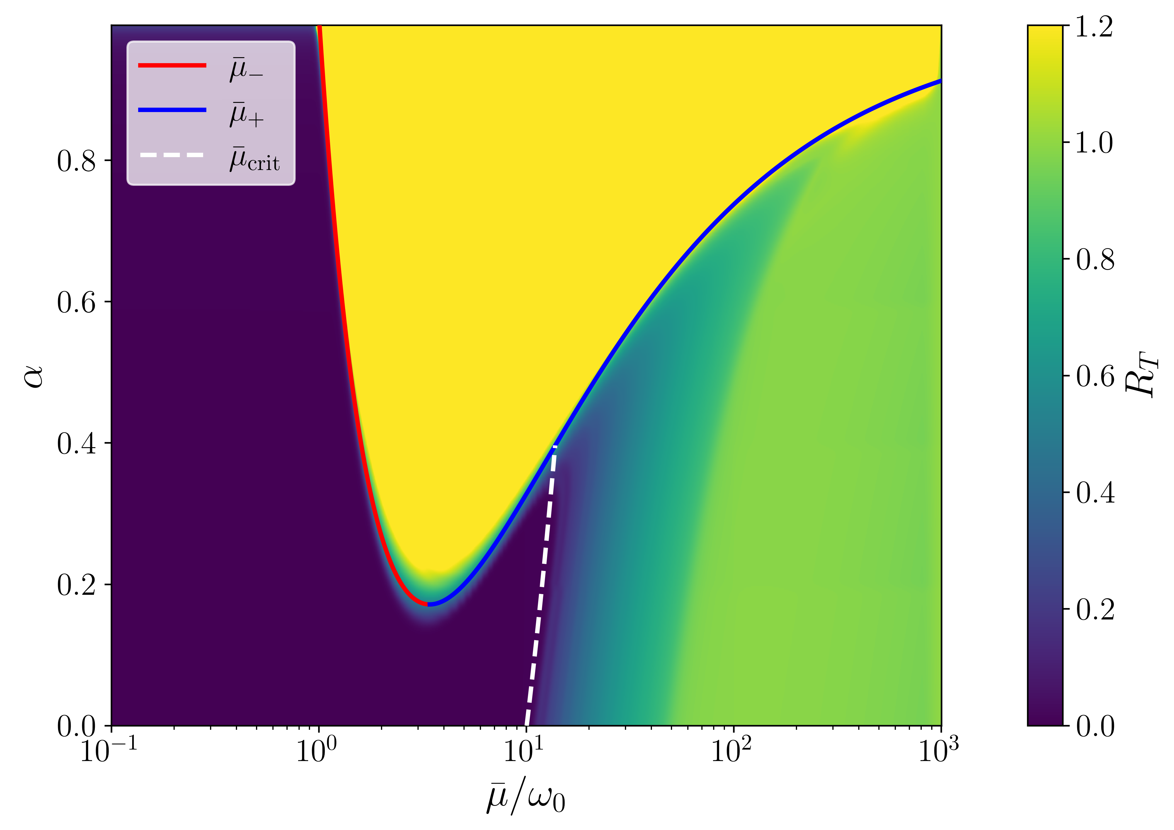
In Fig. 4, for small width $\sigma/\omega_{0}=0.1$, the phase diagram is similar to the two thick-beam case. Increasing the width $\sigma$ shifts the lower boundary $\bar{\mu}_{-}$ to larger values, while the upper boundary $\bar{\mu}_{+}$ shifts less at large $\alpha$. The interval of $\bar{\mu}$ over which bipolar motion is expected becomes narrower. For sufficiently broad spectra, the boundaries $\bar{\mu}_{\pm}$ are no longer real below $\alpha_{\rm crit}$, and no bipolar instability window exists. For example, when $\sigma/\omega_{0}=4$, we find $\alpha_{\rm crit}\simeq 0.61$, which has a large region without a bipolar window. This follows from the crossing criterion of Sec. V.4: $h(\omega)$ develops real crossings only for $\alpha>\alpha_{\rm crit}$. For $\alpha<\alpha_{\rm crit}$, the crossing disappears, and no bipolar instability occurs.

The longitudinal components $P_{z}$ and $\bar{P}_{z}$ diagnose bipolar motion through large-amplitude oscillations, but remain nearly stationary in both stable regimes. They therefore do not distinguish a transversely dephased, i.e., vacuum-like state at low interaction strength, from synchronized motion at large interaction strength. To separate these behaviors, we consider the late-time transverse polarization through the order parameter

where $|P_{\perp}|=\sqrt{P_{x}^{2}+P_{y}^{2}}$ is the transverse component of the total polarization vector $\vec{\mathbb{P}}_{\rm tot}$, and $\langle\cdot\rangle_{\rm late}$ refers to an average over a few cycles at late times of the evolution. For the initial state, the resultant transverse component of the north-south cohorts is

where $Q(\kappa)={\mathcal{I}_{1}(\kappa)}/{\mathcal{I}_{0}(\kappa)},$ and $\delta=2\theta_{\rm mix}$ is the common initial tilt. In the single-cohort and perfectly localized limit, $\alpha=0$ and $Q(\kappa)\to 1$, the instantaneous ratio entering Eq. (44) reduces to $R(t)=P_{\perp}(t)/\sin 2\theta_{\rm mix}$.

The interpretation of $R_{T}$ is straightforward. A value $R_{T}=0$ indicates transverse dephasing, where different frequency modes cancel in the collective sum, while $R_{T}>0$ indicates collective transverse motion. In the presence of spectral crossings, however, $R_{T}$ alone does not distinguish synchronized motion from bipolar oscillations; rather, it distinguishes the two stable regimes.

For $\alpha<\alpha_{\rm crit}$, where no bipolar instability exists, the onset of nonzero $R_{T}$ directly indicates synchronization. A critical value of interaction strength can be obtained from the self-consistency conditions for sustained late-time collective precession. For the two-Lorentzian spectrum, one finds

where $D_{\pm}=(\omega_{r}\mp\omega_{0})^{2}+\sigma^{2}$, with $\omega_{r}$ determined in Appendix E. For $\alpha=0$, substituting the corresponding value of $D_{+}$, this reduces to

Thus, decreasing the initial tilt shifts the synchronization scale to larger interaction strength, with $\bar{\mu}_{\rm crit}\rightarrow\infty$ as $\delta\rightarrow 0$. This agrees with the vanishing mixing angle limit discussed in Ref. [52], where a spectrum with infinite tails remains completely dephased for any finite interaction strength. Note that the order parameter therein was introduced for the stable regime, whereas here $R_{T}$ involves a late-time average and is extended into the bipolar instability region.

We compute $R_{T}$ for crossed and uncrossed spectra, over the $\bar{\mu}/\omega_{0}-\alpha$ plane. Fig. 5 shows the resulting $R_{T}$ together with the synchronization threshold $\bar{\mu}_{\rm crit}$ and the instability boundaries $\bar{\mu}_{\pm}$. At small $\bar{\mu}$, $R_{T}=0$, while at sufficiently large interaction strength the system develops synchronized transverse motion approaching $R_{T}\simeq 1$. Within the bipolar interval, pendular motion gives $R_{T}>1$.

For $\alpha<\alpha_{\rm crit}$, the numerical transition from $R_{T}=0$ to $R_{T}>0$ follows $\bar{\mu}_{\rm crit}$. Immediately above $\alpha_{\rm crit}$, however, the end of the bipolar instability does not coincide with the onset of synchronization. Transverse dephasing persists beyond $\bar{\mu}_{+}$, producing an intermediate region $\bar{\mu}_{+}<\bar{\mu}<\bar{\mu}_{\rm crit}$ until $\bar{\mu}_{\rm crit}$ meets $\bar{\mu}_{+}$. Thus, immediately beyond $\bar{\mu}_{+}$, a linearly stable system need not yet be synchronized.

There is no a priori reason for $\bar{\mu}_{+}$ and the transverse synchronization threshold $\bar{\mu}_{\rm crit}$ to coincide, since they diagnose different transitions. Indeed, in physical systems, different order parameters may be designed to probe different aspects of the system and therefore need not exhibit critical behavior at the same point. A familiar example is a material that undergoes magnetic ordering at one temperature and becomes superconducting only at a lower temperature. Nevertheless Fig. 5 shows that the continued $\bar{\mu}_{\rm crit}$ line meets the bipolar boundary $\bar{\mu}_{+}$ near $\alpha\simeq 0.4$, beyond which the bipolar to synchronized transition occurs directly across the upper boundary.

References

- [1] (2005) The kuramoto model: a simple paradigm for synchronization phenomena. Reviews of Modern Physics 77 (1), pp. 137–185. External Links: Document Cited by: §I, §II.2.
- [2] (2025) Manipulating phases in many-body interacting systems with subsystem resetting. Phys. Rev. Lett. 135, pp. 127103. External Links: Document, Link Cited by: §VII.
- [3] (1996) Absence of self-averaging and universal fluctuations in random systems near critical points. Phys. Rev. Lett. 77, pp. 3700–3703. External Links: Document, Link Cited by: §II.1.
- [4] (2018) Normal-mode Analysis for Collective Neutrino Oscillations. JCAP (12), pp. 019. External Links: Document, 1809.09137 Cited by: §I.
- [5] (2011) Linearized flavor-stability analysis of dense neutrino streams. Phys. Rev. D 84, pp. 053013. External Links: Document, 1107.2308 Cited by: §I.
- [6] (2020) Late-time behavior of fast neutrino oscillations. Phys. Rev. D 102 (6), pp. 063018. External Links: 2005.00459, Document Cited by: §VI.3.
- [7] (2021) Fast Flavor Depolarization of Supernova Neutrinos. Phys. Rev. Lett. 126 (6), pp. 061302. External Links: 2009.03337, Document Cited by: §VI.3.
- [8] (2022) Elaborating the ultimate fate of fast collective neutrino flavor oscillations. Phys. Rev. D 106 (10), pp. 103039. External Links: 2205.05129, Document Cited by: §VI.3.
- [9] (2024) Global density equations for interacting particle systems with stochastic resetting: from overdamped brownian motion to phase synchronization. Chaos 34 (4), pp. 043101. External Links: Document Cited by: §VII.
- [10] (2017) Fast flavor conversions of supernova neutrinos: Classifying instabilities via dispersion relations. Phys. Rev. D 96 (4), pp. 043016. External Links: Document, 1706.03360 Cited by: §I, §I, §III.2.
- [11] (2019) Collisional triggering of fast flavor conversions of supernova neutrinos. Phys. Rev. Lett. 122 (9), pp. 091101. External Links: Document, 1808.06618 Cited by: §VII.
- [12] (2019) Fast Neutrino Flavor Conversion: Collective Motion vs. Decoherence. JCAP 09 (09), pp. 002. External Links: 1906.08794, Document Cited by: §VI.3.
- [13] (2016) Collective neutrino flavor conversion: Recent developments. Nucl. Phys. B 908, pp. 366–381. External Links: Document, 1602.02766 Cited by: §I.
- [14] (2016) Self-induced neutrino flavor conversion without flavor mixing. JCAP 03 (03), pp. 042. External Links: 1602.00698, Document Cited by: §III.2.
- [15] (2019) Continuous versus discontinuous transitions in the d-dimensional generalized kuramoto model: odd d is different. Physical Review X 9 (1), pp. 011002. External Links: Document Cited by: §II.2.
- [16] (2009) Multiple Spectral Splits of Supernova Neutrinos. Phys. Rev. Lett. 103, pp. 051105. External Links: Document, 0904.3542 Cited by: §I.
- [17] (2025) Sufficient and necessary conditions for collective neutrino instability: Fast, slow, and mixed. Phys. Rev. D 112 (12), pp. 123049. External Links: 2505.03886, Document Cited by: §I, §V.4, §V.4, §V.4.
- [18] (2018) Fast Neutrino Flavor Conversion as Oscillations in a Quartic Potential. Phys. Rev. D 97 (2), pp. 023017. External Links: 1709.08671, Document Cited by: §VII.
- [19] (2022) Collective Neutrino Flavor Instability Requires a Crossing. Phys. Rev. Lett. 128 (8), pp. 081102. External Links: 2110.00192, Document Cited by: §I.
- [20] (2007) Analysis of Collective Neutrino Flavor Transformation in Supernovae. Phys. Rev. D 75, pp. 125005. External Links: Document, astro-ph/0703776 Cited by: §III.2, §V.1.
- [21] (2006) Collective neutrino flavor transformation in supernovae. Phys. Rev. D 74, pp. 123004. External Links: Document, astro-ph/0511275 Cited by: §I.
- [22] (2010) Collective Neutrino Oscillations. Ann. Rev. Nucl. Part. Sci. 60, pp. 569–594. External Links: 1001.2799, Document Cited by: §I.
- [23] (2007) Decoherence in supernova neutrino transformations suppressed by deleptonization. Phys. Rev. D 76, pp. 125018. External Links: Document, 0706.2498 Cited by: §VI.3.
- [24] (2020) Stochastic resetting and applications. Journal of Physics A: Mathematical and Theoretical 53 (19), pp. 193001. External Links: Document Cited by: §VII.
- [25] (2011) Diffusion with stochastic resetting. Phys. Rev. Lett. 106, pp. 160601. External Links: Document, Link Cited by: §VII.
- [26] (2024) Theory of neutrino fast flavor evolution. Part I. Linear response theory and stability conditions.. JHEP 08 (08), pp. 225. External Links: 2406.06708, Document Cited by: §I.
- [27] (2025) Theory of neutrino slow flavor evolution. Part I. Homogeneous medium. JHEP 04 (04), pp. 146. External Links: 2412.02747, Document Cited by: §I.
- [28] (2026) Ubiquitous flavor pendulum. Phys. Rev. D 113 (12), pp. 123033. External Links: 2602.02655, Document Cited by: §VII.
- [29] (2025) Steady state of fast-oscillating neutrinos in an inhomogeneous medium. Phys. Rev. D 112 (10), pp. 103011. External Links: 2509.22805, Document Cited by: §VI.3.
- [30] (2014) Kuramoto model of synchronization: equilibrium and nonequilibrium aspects. Journal of Statistical Mechanics: Theory and Experiment 2014 (8), pp. R08001. External Links: Document Cited by: §I, §II.2.
- [31] (2018) Statistical physics of synchronization. Springer, Berlin. External Links: ISBN 978-3-319-70760-8, Document Cited by: §II.2.
- [32] (2006) Self-induced conversion in dense neutrino gases: Pendulum in flavour space. Phys. Rev. D 74, pp. 105010. Note: [Erratum: Phys.Rev.D 76, 029901 (2007)] External Links: Document, astro-ph/0608695 Cited by: §I, §I, §V.1.
- [33] (2017) Fast Pairwise Conversion of Supernova Neutrinos: A Dispersion-Relation Approach. Phys. Rev. Lett. 118 (2), pp. 021101. External Links: Document, 1610.01612 Cited by: §I, §I.
- [34] (2020) Fast oscillations, collisionless relaxation, and spurious evolution of supernova neutrino flavor. Phys. Rev. D 102 (10), pp. 103017. External Links: 2009.09024, Document Cited by: §VI.3.
- [35] (2025) Neutrino Oscillations in Core-Collapse Supernovae and Neutron Star Mergers. Ann. Rev. Nucl. Part. Sci. 75 (1), pp. 399–423. External Links: 2503.05959, Document Cited by: §I.
- [36] (2023) Collisional Flavor Instabilities of Supernova Neutrinos. Phys. Rev. Lett. 130 (19), pp. 191001. External Links: 2104.11369, Document Cited by: §VII.
- [37] (1984) Chemical oscillations, waves, and turbulence. Springer Series in Synergetics, Springer, Berlin, Heidelberg. External Links: ISBN 978-3-642-69689-3 Cited by: §I, §II.2.
- [38] (2026) Dynamical equilibria of fast neutrino flavor conversion. Phys. Rev. D 114 (4), pp. L041306. External Links: 2509.26418, Document Cited by: §VI.3.
- [39] (2026) Analytical approach to subsystem resetting in generalized kuramoto models. Phys. Rev. E 114, pp. 024108. External Links: Document, Link Cited by: §VII.
- [40] (2025) Finite-size fluctuations for stochastic coupled oscillators: a general theory. External Links: 2510.02448, Link Cited by: §II.2.
- [41] (2024) Kuramoto model subject to subsystem resetting: how resetting a part of the system may synchronize the whole of it. Phys. Rev. E 109, pp. 064137. External Links: Document, Link Cited by: §VII.
- [42] (2026) Synchronization with annealed disorder and higher-harmonic interactions in arbitrary dimensions: when two dimensions are special. APS Open Sci. 1, pp. 000069. External Links: Document, Link Cited by: §II.2.
- [43] (2020) Dynamic fast flavor oscillation waves in dense neutrino gases. Phys. Lett. B 800, pp. 135088. External Links: 1909.05225, Document Cited by: §VI.3.
- [44] (2016) Supernova Neutrinos: Production, Oscillations and Detection. Riv. Nuovo Cim. 39 (1-2), pp. 1–112. External Links: Document, 1508.00785 Cited by: §I.
- [45] (2022) Fast neutrino flavor instability and neutrino flavor lepton number crossings. Phys. Rev. D 105 (10), pp. L101301. External Links: 2103.15267, Document Cited by: §I.
- [46] (2022) Time-Dependent and Quasisteady Features of Fast Neutrino-Flavor Conversion. Phys. Rev. Lett. 129 (26), pp. 261101. External Links: 2206.04097, Document Cited by: §VI.3.
- [47] (2026) NIST digital library of mathematical functions. Note: https://dlmf.nist.gov/Release 1.2.7 of 2026-06-15 Cited by: Appendix A, Appendix A.
- [48] (2022) Neutrino Flavor Pendulum Reloaded: The Case of Fast Pairwise Conversion. Phys. Rev. Lett. 128 (12), pp. 121102. External Links: 2109.14627, Document Cited by: §VII.
- [49] (1992) Neutrino oscillations at high densities. Phys. Lett. B 287, pp. 128–132. External Links: Document Cited by: §I.
- [50] (1960) Electrostatic instabilities of a uniform non-maxwellian plasma. The Physics of Fluids 3 (2), pp. 258–265. External Links: ISSN 0031-9171, Document, Link Cited by: §V.4.
- [51] (2007) Self-induced decoherence in dense neutrino gases. Phys. Rev. D 75, pp. 083002. External Links: Document, hep-ph/0701182 Cited by: §VI.3.
- [52] (2010) Synchronization versus decoherence of neutrino oscillations at intermediate densities. Phys. Rev. D 82, pp. 125004. External Links: Document, 1006.0002 Cited by: Appendix E, §I, §VI.3.
- [53] (2021) Neutrino fast flavor instability in three dimensions. Phys. Rev. D 104 (10), pp. 103023. External Links: 2109.08631, Document Cited by: §VI.3.
- [54] (2005) Speed-up of neutrino transformations in a supernova environment. Phys. Rev. D 72, pp. 045003. External Links: Document, hep-ph/0503013 Cited by: §I.
- [55] (2009) The multi-angle instability in dense neutrino systems. Phys. Rev. D 79, pp. 105003. External Links: Document, 0803.4319 Cited by: §I.
- [56] (1993) General kinetic description of relativistic mixed neutrinos. Nucl. Phys. B 406, pp. 423–451. External Links: Document Cited by: §I.
- [57] (2000) From Kuramoto to Crawford: Exploring the onset of synchronization in populations of coupled oscillators. Physica D 143 (1–4), pp. 1–20. External Links: Document Cited by: §I, §II.2.
- [58] (2021) New Developments in Flavor Evolution of a Dense Neutrino Gas. Ann. Rev. Nucl. Part. Sci. 71, pp. 165–188. External Links: 2011.01948, Document Cited by: §I.
- [59] (2024) Neutrinos from dense environments: Flavor mechanisms, theoretical approaches, observations, and new directions. Rev. Mod. Phys. 96 (2), pp. 025004. External Links: 2301.11814, Document Cited by: §I.
- [60] (1995) Lack of self-averaging in critical disordered systems. Phys. Rev. E 52, pp. 3469–3484. External Links: Document, Link Cited by: §II.1.
- [61] (2021) Collective fast neutrino flavor conversions in a 1D box: Initial conditions and long-term evolution. Phys. Rev. D 104 (10), pp. 103003. External Links: 2108.09886, Document Cited by: §VI.3.
- [62] (2023) Collisional flavor instability in dense neutrino gases. Phys. Rev. D 108 (8), pp. 083002. External Links: 2212.03750, Document Cited by: §VII.