Schatten norms and determinants of linear combinations of matrix tensor powers via virtual representations Note: This work was supported by the National Research, Development and Innovation Office of Hungary (NKFIH) via the grants ADVANCED_25 152599, K 146380 and EXCELLENCE 151342, and by the Ministry of Culture and Innovation and the NKFIH within the Quantum Information National Laboratory of Hungary (Grant No. 2022-2.1.1-NL-2022-00004).
Abstract
Let where and are fixed, while grows. Direct computation of determinants or Schatten norms of is exponential in . For a single tensor power these quantities are elementary, and even the determinant of a generic two-term combination admits a reduction to polynomially many scalar factors; however, no analogous elementary reduction is available for three or more terms.
We give an exact representation-theoretic method which, for fixed and , computes , , and determinants in polynomial time in . Schur–Weyl duality yields a simultaneous block decomposition, while Jacobi–Trudi identities in the Grothendieck ring replace Schur modules by signed combinations of tensor products of symmetric powers.
For , each irreducible contribution reduces to the difference of two explicitly computable symmetric-power terms, leading to an open-source implementation. In a single-thread CPU benchmark, a genuine three-term trace-norm problem with is evaluated in about seconds, whereas just storing the unreduced matrix would require approximately bytes. Direct and reduced computations agree to relative error below throughout their common range .
Keywords:
Tensor powers, quantum hypothesis testing, Schatten norms, Schur–Weyl duality, representation rings, Jacobi–Trudi identity2020 MSC
15A69 , 20G05 , 65F30 , 81P451 Introduction
For fixed matrices and scalars , consider
| (1) |
The order of is , and a dense representation contains entries. Nevertheless, the cases , , and have rather different characters.
For one tensor-power term, many standard quantities are immediate. For example,
| (2) |
The determinant of a two-term combination is still elementary in a useful sense. Suppose that is invertible, put , and let be the eigenvalues of , repeated with algebraic multiplicity. Factoring out and grouping the eigenvalues of by occupation numbers gives
| (3) |
Thus, for fixed , only distinct scalar factors are needed. There is no analogous factorization for three generic matrices: a third term cannot in general be expressed through the spectrum of one relative matrix. This elementary contrast is one indication that the first genuinely difficult case begins with three tensor-power terms.
Quantum hypothesis testing gives a second indication. The minimum Bayesian error probability for distinguishing two states and , with prior probabilities and , is
| (4) |
see [5, 6]. Exact finite-copy evaluation is already nontrivial, but its asymptotic exponential rate has the single-letter quantum Chernoff formula [1]
| (5) |
Now let the null hypothesis contain two states, and , with prior weights and , while the alternative consists of a state with weight . The optimal Bayesian error becomes
| (6) |
This is the first three-term trace-norm problem. In contrast with the simple case, no general single-letter formula for its asymptotic exponent is known; indeed, a natural candidate suggested by the classical theory was disproved in [8] by one of the present authors and two collaborators. The same three-term threshold therefore appears both in elementary determinant algebra and in the motivating quantum information problem.
The repeated tensor power in (1) has much more symmetry than a generic matrix. Schur–Weyl duality makes this symmetry visible: the map splits into polynomial -representations indexed by partitions of . This observation alone is not yet a numerical method, because explicit matrices for general Schur functors are cumbersome. Our main point is that the required irreducible matrices need not be constructed. The Jacobi–Trudi identity expresses their classes as virtual combinations of tensor products of symmetric powers. Since the th power of the Schatten -norm is additive under orthogonal direct sums, identities in the representation ring become exact signed identities of numerical quantities. For determinants and characteristic polynomials, direct-sum additivity is replaced by multiplicativity, and virtual coefficients become integer exponents.
Two technical points are essential. First, singular values are preserved by unitary, not arbitrary, changes of basis. We therefore obtain the block decomposition from the compact group and then extend the same fixed unitary intertwiner to all of . Second, a virtual representation is a formal difference, not a matrix with negative blocks. It is useful here only because the functional being evaluated is additive on orthogonal direct sums.
The present implementation supports and matrices. The reproducible benchmarks in Section 8 use a single CPU thread and include both two-term and genuinely three-term trace-norm expressions. For the three-term family, a fresh-process evaluation at takes about seconds. Direct dense storage at this tensor power would already require approximately bytes. At , where brute-force comparison is still feasible on the benchmark machine, the reduced method agrees with direct evaluation to relative error and its warm evaluation is about times faster. The implementation data extend to for inputs; at that power the unreduced matrix has order
whereas the largest virtual block has order only .
Main contributions
The main contribution is the development of a practical new method for the mentioned kind of computations involving large tensor powers. In particular:
- (i)
We prove a simultaneous unitary Schur–Weyl block decomposition valid for every matrix , including singular and nonnormal matrices (Theorem 2.1), and show how representation-ring identities yield exact identities for additive Schatten functionals and, separately, for multiplicative invariants such as determinants and characteristic polynomials (Propositions 3.1 and 3.3).
- (ii)
We combine determinant twists with Jacobi–Trudi to give a fixed- master formula involving only symmetric powers (Theorem 4.1). For each Schur contribution is a difference of two explicitly computable terms.
- (iii)
We give an implementation-level description of the sparse monomial tables, coefficient matrices, cache structure, aggregation of identical virtual blocks, and the online evaluation algorithm.
- (iv)
We establish the dense worst-case complexity , give exact block-size and memory comparisons, report reproducible CPU benchmarks for two- and three-term trace-norm problems, and formulate numerical stability diagnostics for cancellation in the virtual formula.
The original motivation was the composite-hypothesis problem above. An earlier project, carried out with Sloan Nietert, treated the case in Wolfram Mathematica [12]. That dimension is exceptional: after a determinant twist every relevant irreducible representation is a symmetric power. Dimension three is the first case in which virtual subtraction is genuinely needed. The present paper develops that case explicitly and places it in a construction valid for arbitrary fixed .
2 A unitary decomposition valid for arbitrary matrices
We first isolate the passage from the compact group to arbitrary complex matrices. This both fixes the Hilbert-space geometry needed for singular values and explains why the final formulas apply beyond unitary or invertible inputs.
Let be a partition of , padded with zeros, and write for the condition that at most parts are nonzero. Let denote the Schur module of highest weight , and let be the Specht module of the symmetric group . Set
One convenient form of the hook-length formula is
| (7) |
Theorem 2.1 (Simultaneous unitary block decomposition).
For every , there are Hilbert-space structures on the Schur modules and a unitary map
such that, for every ,
| (8) |
The map depends on and , but not on .
Proof.
Restrict first to . The actions of and on commute. Complete reducibility for the compact group, together with Schur–Weyl duality, gives the orthogonal decomposition
After choosing orthonormal bases, the corresponding intertwiner is unitary, and (8) holds for every .
Differentiate the intertwining relation along one-parameter subgroups of . It follows that intertwines the derived representations of the Lie algebra . Since the complex linear span of is , it intertwines the complexified derived representations as well. The group is connected, so the relation follows for every invertible complex matrix. Equivalently, one may use that every invertible complex matrix has a logarithm and exponentiate the derived relation.
Finally, both sides of (8) are matrices whose entries are polynomials in the entries of . Since is dense in , the identity extends to singular matrices. ∎
Remark 2.2 (Why rather than or ?).
Starting from gives the correct algebraic decomposition but does not by itself supply an orthogonal one: a general intertwining matrix does not preserve singular values. Compactness of gives invariant Hermitian inner products and hence a unitary intertwiner. The group is compact as well, but is more natural here because determinant characters remain visible. They are exactly what separates polynomial -representations that become equivalent after restriction to . Theorem 2.1 then transfers the unitary decomposition from to all complex matrices.
For , the Schatten -functional is
For this is the th power of a quasi-norm; its direct-sum additivity is unchanged.
Corollary 2.3.
Let , , and . Then
| (9) |
Proof.
Remark 2.4 (The operator norm).
For , an actual orthogonal decomposition still gives
The virtual-representation step below, however, relies on additivity and does not extend to the maximum. We therefore restrict the virtual formula and its algorithmic consequences to .
3 Additive spectral functionals and virtual representations
We now explain precisely how a representation-ring identity can be used without constructing an irreducible representation.
Fix , coefficients , and . If is a homogeneous polynomial representation of , choose a Hermitian inner product for which is unitary and define
| (10) |
The polynomial map is defined at singular as well.
Proposition 3.1.
The quantity depends only on the isomorphism class of and is additive:
Consequently, it extends uniquely to a group homomorphism
from the Grothendieck group of finite-dimensional polynomial representations.
Proof.
Two isomorphic polynomial representations restrict to equivalent unitary representations of . Their equivalence can therefore be implemented by a unitary intertwiner. By the same complexification and polynomial-continuation argument as in Theorem 2.1, that intertwiner works for every . Hence the matrices in (10) are unitarily similar and have the same singular values.
For a direct sum,
so additivity follows from direct-sum additivity of the th power of the Schatten functional. The universal property of the Grothendieck group gives the extension. ∎
Remark 3.2.
If in the representation ring, then
This statement concerns the value of an additive functional. It does not assert that is obtained by deleting a visible matrix block from in the bases used for computation.
3.1 Multiplicative invariants
The representation-ring method is not limited to additive functionals. For a polynomial representation , define
| (11) |
Unlike , this functional is multiplicative under direct sums:
Thus a virtual coefficient becomes an exponent rather than a scalar coefficient.
Proposition 3.3.
Suppose that
| (12) |
in the Grothendieck group of polynomial representations. Then
| (13) |
In particular, whenever all factors with are nonzero,
| (14) |
The same statements hold with replaced by the characteristic polynomial
Proof.
Separate the positive and negative parts of (12). The definition of the Grothendieck group gives an isomorphism
possibly after adding the same auxiliary representation to both sides. Apply the determinant to the corresponding direct-sum matrices, treating the entries of the and the as indeterminates. The auxiliary factor is not the zero polynomial—set , , and all other —so it cancels in the polynomial ring. This gives (13). Division gives (14) under the stated nonvanishing condition. The argument with is identical. ∎
Remark 3.4.
The integrality of the coefficients in (12) is exactly what makes negative coefficients harmless for a multiplicative invariant: they become negative integer exponents. At exceptional inputs a direct quotient may have the indeterminate form . The cross-multiplied identity remains valid there; numerical evaluation can use a small generic perturbation and a limit, while symbolic evaluation can cancel common polynomial factors before substitution.
4 Jacobi–Trudi reduction to symmetric powers
Let be a partition. Put
Then , so , and
| (15) |
The identity remains meaningful for singular : both sides are polynomial functions of its entries.
For , write in the representation ring, put , and put for . The Jacobi–Trudi identity [7, Ch. I] gives
| (16) |
Expanding the determinant yields
| (17) |
where a tensor product containing a negative symmetric power is interpreted as zero.
For , define the polynomial representation
| (18) |
again setting it equal to zero if one of the exponents is negative. When , the empty tensor product is the one-dimensional trivial representation.
Theorem 4.1 (Master formula).
Proof.
Remark 4.2.
Corollary 4.3 (Determinants from the master decomposition).
Put
Then
| (20) |
and each Schur factor satisfies
| (21) |
For generic input matrices, the factors on the left are nonzero and (21) gives as a quotient.
5 The explicit formulas for and
5.1 Why the case is exceptional
For , every has the form with , and
| (22) |
There is no nontrivial Jacobi–Trudi subtraction. Thus symmetric powers and determinant characters already give every block directly. This special feature motivated the earlier Mathematica implementation [12], but it does not persist in dimension three.
5.2 The first virtual case: matrices
Let and set
The Jacobi–Trudi determinant gives
| (23) |
where the second term is zero when . Therefore
| (24) |
Together with (9), this is the formula used by the implementation.
6 Explicit matrices for symmetric powers
It remains to construct efficiently. Let
The normalized occupation-number vectors indexed by form an orthonormal basis of . Its dimension is
| (25) |
For , let be the set of nonnegative integer matrices whose row sums are and whose column sums are . Write
Proposition 6.1.
In the normalized occupation-number basis,
| (26) |
Proof.
Expand between the normalized symmetrizations of tensor words with occupation vectors and . A pair of words contributes the monomial , where counts positions at which the input letter is and the output letter is . For fixed , the number of such assignments is . The two normalization factors cancel the and leave (26). ∎
For fixed and , the sets of exponent arrays and the coefficients do not depend on . They can therefore be precomputed and stored sparsely. Evaluating then reduces to evaluating a fixed list of monomials in the entries of and accumulating them into the prescribed matrix positions. The same precomputed table is reused for every matrix in a numerical experiment.
6.1 Sparse coefficient tables and online evaluation
Formula (26) is suitable for direct implementation, but it is wasteful to enumerate the contingency tables every time a new numerical matrix is supplied. The matrix-independent part can be extracted completely. Let
and fix an ordering of . For , define the monomial vector by
After flattening the symmetric-power matrix in a fixed row-major order, Proposition 6.1 gives a sparse matrix , independent of , such that
| (27) |
The rows of are indexed by pairs of occupation vectors, and a nonzero coefficient in column is obtained by summing over the exponent matrices with flattened exponent vector , row sums , and column sums .
The implementation stores the ordered exponent array and in sparse compressed form. At run time, all monomials are evaluated by vectorized power and product operations, followed by one sparse matrix–vector product and a reshape. Thus symbolic expressions are absent from the online phase. For a fixed query , each matrix is cached the first time degree is requested and is then reused across all partitions and Jacobi–Trudi terms.
For , one can also aggregate identical virtual blocks before any dense matrix is formed. For , formula (24) contributes the key with integer weight and, when , the key with weight . Let be the total weight after summing over all partitions of . Then
| (28) |
Zero coefficients are discarded. This aggregation is exact integer arithmetic and avoids repeated evaluation of coincident positive and negative terms.
The online algorithm can therefore be summarized as follows.
Algorithm 1 (weighted Schatten functional for ). Given , matrices , and coefficients :
- 1.
enumerate the partitions with at most three parts, compute , and assemble the integer dictionary ;
- 2.
determine all symmetric degrees required by the nonzero keys, evaluate and cache using (27);
- 3.
for each nonzero key, form the weighted dense block in (28), compute its singular values, and add to the accumulator;
- 4.
take the th root after checking the cancellation diagnostics in Section 8.
The matrix-independent tables are an offline resource. Their generation, loading, and caching must be distinguished from repeated online evaluation in any meaningful benchmark. The public implementation follows this separation and exposes a class-level interface for block decompositions and weighted Schatten norms [9].
7 Algorithmic complexity
For clarity, the general- evaluation of (19) consists of the following steps.
- 1.
Enumerate the partitions with and compute from (7).
- 2.
Remove the last part and form .
- 3.
For each nonzero Jacobi–Trudi term , obtain the required symmetric powers from the cache, take their Kronecker products, and multiply by .
- 4.
Form , compute its singular values, and add the signed th powers with weight .
- 5.
Aggregate the contributions and take the th root.
We give a deliberately conservative dense-arithmetic bound for the online phase. The number of partitions of with at most parts is . After the determinant twist, each Jacobi–Trudi term has at most symmetric factors, and there are at most such terms. For fixed and degrees ,
Consequently, the largest dense matrix in a Jacobi–Trudi term has order
| (29) |
Theorem 7.1.
For fixed , fixed , and , a direct dense implementation of (19) has worst-case online arithmetic complexity
| (30) |
and peak dense-matrix storage
| (31) |
apart from the matrix-independent sparse coefficient tables.
Proof.
There are partitions and, for fixed , only a constant number of Jacobi–Trudi terms per partition. Dense singular-value decomposition of a matrix of order (29) costs . Processing the terms sequentially gives the asserted storage bound. Caching the symmetric powers adds lower-order dense storage for fixed and does not change the exponent. ∎
Dense determinant evaluation by elimination has the same cubic arithmetic order. At generic inputs, where the quotient form of Corollary 4.3 is directly evaluable, determinants therefore obey the same worst-case polynomial bound. Characteristic polynomials can also be recovered from the multiplicative identities, although their full symbolic expansion may of course be substantially more expensive than a single numerical determinant.
For , the largest block has order , the dense SVD cost per block is , and the number of partitions is . The resulting bound is , with peak dense storage . Most partitions produce much smaller blocks, so this worst-case exponent is not a prediction of moderate- wall-clock behavior.
Remark 7.2.
The qualification “for fixed ” is essential. Both the number of Jacobi–Trudi terms and the polynomial degree in (30) grow with . The result is a fixed-dimension polynomial algorithm, not a polynomial-time algorithm when is part of the input.
8 Numerical realization, benchmarks, and validation
The formulas have been implemented in the open-source Python package tensorpow [9]. The benchmarked release, version 0.3.0, supports and inputs, with representation data through degree for the former and degree for the latter. The data can be cached locally before a computation, and the implementation never forms the full matrix. The package also provides an optional GPU backend for the dense singular-value decompositions; the benchmarks below use the CPU backend so that all reported timings refer to one controlled hardware configuration.
8.1 Exact size comparison
Table 1 gives a machine-independent comparison for . The full storage column assumes dense complex128 data, namely 16 bytes per entry. The maximum virtual-block order is obtained from
where the second term is included only for . These values do not depend on a particular matrix or software implementation.
| full order | full dense storage | partitions | max. block order | |
|---|---|---|---|---|
| 9 | B | 12 | 315 | |
| 12 | B | 19 | 784 | |
| 15 | B | 27 | 1620 | |
| 18 | B | 37 | 3025 | |
| 21 | B | 48 | 5148 | |
| 24 | B | 61 | 8281 | |
| 26 | B | 70 | 11025 | |
| 30 | B | 91 | 18496 |
Already at , direct dense storage would require several terabytes, whereas the largest reduced block has order below . At , the reduction replaces a matrix with about entries by 91 signed block contributions, none larger than .
8.2 Reproducible CPU benchmark
The benchmark suite compares the virtual-block method with direct Kronecker construction wherever the latter remains feasible. It evaluates two fixed families,
| (32) | ||||
| (33) |
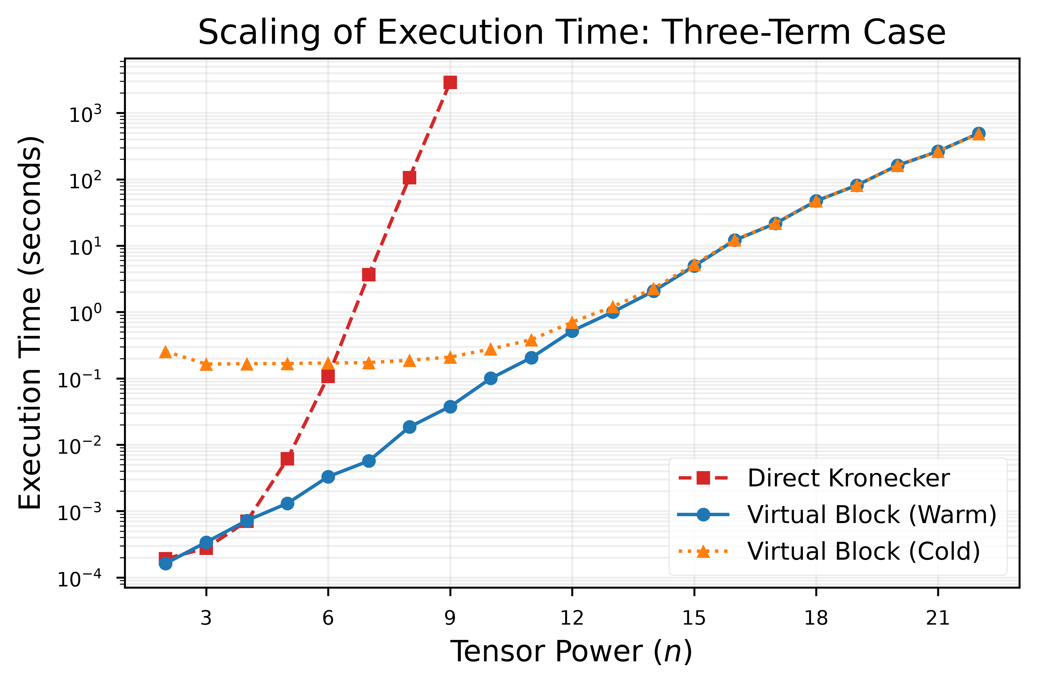
where are independently generated random density matrices from the fixed seed . Each state is obtained as from a complex Gaussian matrix . The direct method explicitly constructs the Kronecker powers and computes a dense SVD. The virtual-block method is measured both in a warm mode, where a TensorPowerCalculator instance and cached data are reused, and in a cold-process mode, where each measurement starts a fresh Python process.
The measurements were made on CachyOS Linux on an Intel Core i5-14600KF at base clock speed with 32 GB DDR5-6000 CL36 memory. All BLAS/LAPACK thread environment variables were fixed to one. The software stack was Python 3.13.14, tensorpow 0.4.2, NumPy 2.5.2, SciPy 1.18.0, and OpenBLAS 0.3.34. Representation files were cached before timing, so no network I/O is included. Warm virtual-block timings use three repetitions after one warm-up; Table 2 reports their medians and median absolute deviations (MAD). Direct and cold-process measurements use one repetition at each . The complete raw output, environment metadata, tables, and plots are available on GitHub [10], while the precomputed symmetric representations are archived on Zenodo [11].
| Direct, 3-term | VB warm, 2-term | VB warm, 3-term | VB cold, 3-term | Rel. err. | |
|---|---|---|---|---|---|
| 5 | |||||
| 7 | |||||
| 8 | |||||
| 9 | |||||
| 12 | — | — | |||
| 15 | — | — | |||
| 18 | — | — | |||
| 22 | — | — |
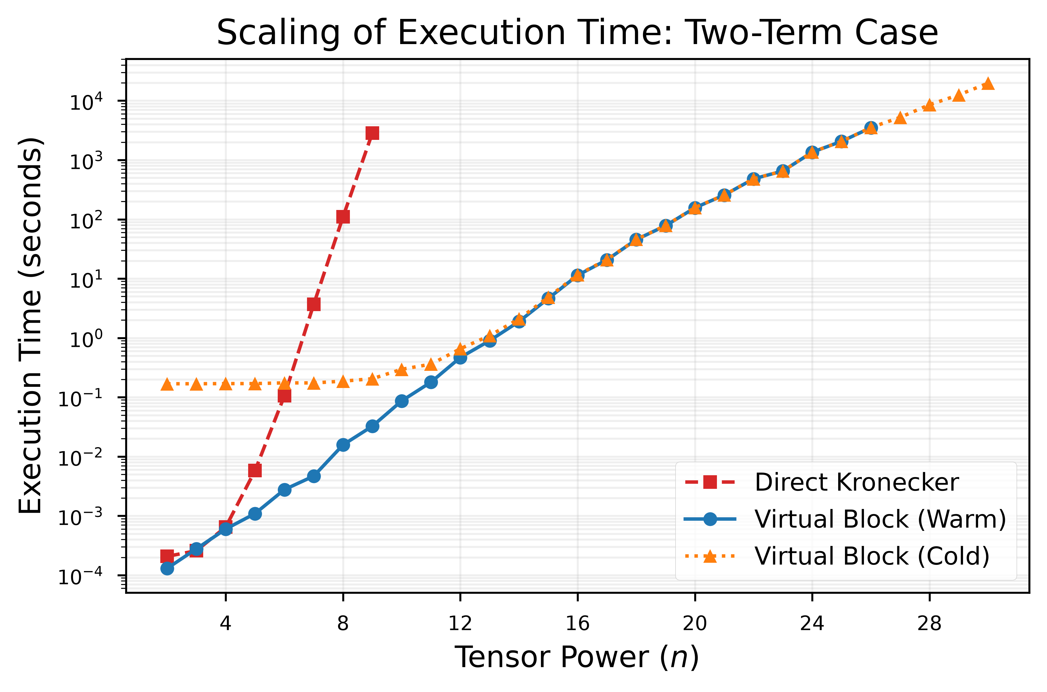
Figure 1 shows the full available three-term series. The direct method becomes prohibitively expensive between and : its runtime rises from about seconds to about seconds, whereas the warm virtual-block time at is seconds. Agreement through the entire overlap range is at relative error at most . Beyond the direct range, the three-term virtual-block calculation remains below one second at , below five seconds at , and below one minute at . At the full matrix would contain approximately entries and occupy about bytes in complex double precision.
.
The two-term and three-term virtual-block timings are close because the sizes and multiplicities of the representation-theoretic blocks are determined by and , not by the number of summands. At , for example, the warm medians are about and seconds, respectively. The additional term therefore adds only a small overhead in this test family, even though it changes the algebraic character of the problem: unlike the two-term determinant reduction discussed in the introduction, the three-term trace norm has no comparable elementary spectral factorization.
The optional GPU backend changes only the dense SVD stage and not the representation-theoretic reduction. While the CPU benchmark establishes a rigorous, machine-independent baseline, delegating the SVD stage to the GPU in version 0.4.2 provides an approximately 9-fold () speedup for the largest reduced blocks. Note that GPU timings are not combined with the CPU data in Table 2; when utilizing the GPU, device memory can eventually become the limiting resource for the largest blocks even if host memory remains sufficient. This speedup was achieved with an NVIDIA 5070 that has 12 GB of VRAM, while other components and packages were kept the same. The VRAM was sufficient until with partial offloading to RAM.
8.3 Cancellation and numerical stability
Exactness in the representation ring does not imply numerical well-conditioning. For a fixed , put
Whenever , define the a posteriori cancellation indicator
| (34) |
Large values signal loss of relative accuracy in floating-point subtraction. For , this is the sum of the two nonnegative terms in (24) divided by the absolute value of their difference. An analogous global indicator is obtained from the aggregated terms in (28).
The following safeguards are appropriate in both testing and production runs:
- 1.
validate all feasible small against direct Kronecker construction;
- 2.
include random unitary, nonnormal, ill-conditioned, singular, and exactly commuting test matrices;
- 3.
report both absolute and relative residuals, since the true value may be close to zero;
- 4.
monitor (34) and repeat poorly conditioned cases in extended precision;
- 5.
use pairwise or compensated summation for the signed scalar contributions;
- 6.
use scaling or logarithmic bookkeeping for large determinant powers, and never silently truncate a substantially negative computed value of to zero.
The benchmark distinguishes cold-start loading from warm repeated evaluation. This separation is particularly important in hypothesis-testing searches, where many matrix families are evaluated at the same tensor powers and the matrix-independent representation data are amortized.
9 Discussion and outlook
The method separates three structures that are easily conflated. Schur–Weyl duality supplies an orthogonal block decomposition; the representation ring supplies virtual identities among additive or multiplicative block functionals; and the symmetric-power formula supplies concrete matrices. These explain both the generality and the limitations of the construction.
Starting with is essential for Schatten norms, but imposes no unitary restriction on the inputs. The same unitary intertwiner works for by complexification and for singular matrices by polynomial continuation. Determinant characters are equally structural: removing the last row of a partition reduces the Jacobi–Trudi determinant from size to at most , thereby improving the block-size exponent.
The fixed-dimension polynomial reduction is exact, but the present dense implementation is not intended to be optimal. Structure-preserving SVDs, randomized methods with certified error bounds, and problem-specific sparsity may extend the practical range. The current software already permits the SVD stage to be carried out on a compatible GPU, while leaving the reduction and its exact formulas unchanged. The matrix-independent representation data can be cached locally and distributed as a separate versioned resource. Other direct-sum additive spectral functionals can be treated by the same virtual identities. Multiplicative invariants lead to products with integer exponents. In contrast, the operator norm and other functionals governed by a maximum rather than a sum cannot be recovered from a formal virtual difference alone.
The benchmark release records the random seed, cold and warm timings, software and BLAS/LAPACK information, thread settings, raw repetitions, and direct-method residuals, and is archived independently of the manuscript [10]. This provides a reproducible performance baseline without fitting an empirical complexity exponent over a short range of ; the asymptotic statement remains the exact worst-case bound of Theorem 7.1.
From the viewpoint of the motivating application, the main value of the method is access to finite-copy expressions such as (6), precisely where three or more tensor-power terms prevent the elementary reductions available for one term or for a two-term determinant. The representation-theoretic compression does not supply a single-letter asymptotic formula by itself, but it makes numerical exploration of that difficult regime possible far beyond brute force.
Acknowledgements
The authors thank Sloan Nietert, who developed the earlier Wolfram Mathematica realization of the method under M.W.’s supervision. That implementation is archived at Zenodo [12].
Author contributions.
M.W. conceived the representation-theoretic approach, including the use of virtual representations and symmetric-power realizations. Under his supervision, M.Á.J., for his MSc thesis, developed the explicit realization, designed and implemented the algorithms and software, and carried out the numerical experiments. Both authors contributed to the mathematical presentation, verified the final manuscript, and accept responsibility for its contents. The authors are listed alphabetically.
Code and data availability
The Python implementation tensorpow is available from its GitHub repository and from the Python Package Index [9]. The benchmark data, reproducibility metadata, tables, and plotting outputs used in Section 8.2 are archived at Zenodo [10]. The earlier Mathematica implementation for matrices is archived separately at Zenodo [12].
Declaration of generative AI and AI-assisted technologies in the manuscript preparation process
During the preparation of this work, the authors used OpenAI ChatGPT to assist in restructuring material from the MSc thesis into article form and to improve the organization, language, and readability of the manuscript. The authors reviewed, verified, and edited all mathematical statements, proofs, references, and numerical claims and take full responsibility for the content of the publication.
References
- [1] K. M. R. Audenaert, J. Calsamiglia, R. Muñoz-Tapia, E. Bagan, Ll. Masanes, A. Acín, and F. Verstraete, Discriminating states: The quantum Chernoff bound, Phys. Rev. Lett. 98 (2007), 160501. https://doi.org/10.1103/PhysRevLett.98.160501.
- [2] R. Bhatia, Matrix Analysis, Graduate Texts in Mathematics 169, Springer, New York, 1997.
- [3] W. Fulton and J. Harris, Representation Theory: A First Course, Graduate Texts in Mathematics 129, Springer, New York, 1991.
- [4] R. Goodman and N. R. Wallach, Symmetry, Representations, and Invariants, Graduate Texts in Mathematics 255, Springer, Dordrecht, 2009.
- [5] C. W. Helstrom, Quantum Detection and Estimation Theory, Academic Press, New York, 1976.
- [6] A. S. Holevo, Statistical decision theory for quantum systems, J. Multivariate Anal. 3 (1973), 337–394. https://doi.org/10.1016/0047-259X(73)90028-6.
- [7] I. G. Macdonald, Symmetric Functions and Hall Polynomials, 2nd ed., Oxford Mathematical Monographs, Oxford University Press, Oxford, 1995.
- [8] M. Mosonyi, Z. Szilágyi, and M. Weiner, On the error exponents of binary quantum state discrimination with composite hypotheses, IEEE Trans. Inform. Theory 68 (2022), 1032–1067. https://doi.org/10.1109/TIT.2021.3125683.
- [9] M. Á. Juhász, tensorpow: Norms and block decompositions for and tensor powers, version 0.4.2, Python software, 2026. https://pypi.org/project/tensorpow/; https://github.com/juhaszmartin/tensorpow.
- [10] M. Á. Juhász, tensorpow_benchmark: Reproducible benchmark protocol and results for tensorpow, GitHub repository, 2026. https://github.com/juhaszmartin/tensorpow_benchmark.
- [11] M. Á. Juhász, Precomputed symmetric representations for tensorpow, Zenodo, 2026, record 21862985. https://zenodo.org/records/21862985.
- [12] M. Weiner and S. Nietert, tensor-powers_of_2x2_matrices: First release, version 1.0, Wolfram Mathematica software, Zenodo, 2025. https://doi.org/10.5281/zenodo.15042414.
- [13] H. Weyl, The Classical Groups: Their Invariants and Representations, 2nd ed., Princeton University Press, Princeton, NJ, 1946.