跳到论文正文
W Papers独立论文阅读器 arXiv:2609.04084 论文正文 计算阅读时间 · 0%
引用这篇论文根据当前论文元数据生成,正式投稿前建议核对。


License: arXiv.org perpetual non-exclusive license
arXiv:2609.04084v1 [math.OC] 03 Sep 2026

Transversality Conditions for Boundary Constraints Defined by Differential Equations

I. M. Ross
Naval Postgraduate School, Monterey, CA 93943
††thanks: Distinguished Professor, Department of Mechanical and Aerospace Engineering.
Abstract

What are the transversality conditions for an optimal control problem when the boundary conditions are defined by differential equations? This seemingly bizarre question is motivated by trajectory optimization problems in the NN-body system. The question, however, is more fundamental and goes beyond problems in astrodynamics to nonintegrable dynamical systems in general. The main contribution of this paper is the development of generic initial- and final-time transversality conditions for optimal control problems whose boundary conditions are defined in terms of differential equations with side conditions. The mathematical definition of differential boundary conditions are part of the foundations developed in this paper. To support the new fundamentals, the concept of coordinated/uncoordinated clock times and weak adjoint covectors are introduced. In the case of uncoordinated clock times, the new transversality conditions reveal that there exists a special situation where a weak adjoint covector is orthogonal to the vector field of the boundary differential equation. This condition is sharply different from the classical statement of orthogonality with respect to the endpoint manifold. The theorems developed in this paper are generic. An application of the theorems to several cases in the three-body problem are described in separate papers.

1 A Motivating Problem

We begin with a suite of practical astrodynamics problems for the sole purpose of providing a context for an unconventional mathematical formulation of boundary conditions. In terms of the specific objectives of this paper, it is not necessary for the reader to have any knowledge of astronautics. With this perspective in mind, consider the problem of optimally transferring a spacecraft from an initial orbit to a final orbit in the restricted three-body problem[1, 2]. Candidate initial and final orbits are depicted in Fig. 1.

Refer to caption
Figure 1: Practical examples of orbits that cannot be naturally defined in terms of algebraic equations (adapted from [11], with permission).

Obviously, this problem definition is superficially similar to a text-book two-body optimal control problem[5, 6, 3, 4]. In the classic two-body problem, the initial- and final orbits are conics: circles, ellipses, hyperbolas etc. Such geometric shapes can be described in terms of algebraic equations or so-called element sets[7]. The element sets are integrals of motion. In the three-body problem, the orbits, such as the ones shown in Fig. 1, are not describable in terms of similar integrals of motion. In fact, the prior sentence is essentially a statement of the famous Bruns-Poincaré theorem of impossibility[8, 10, 9]. Hence, it follows that a major difference between a three-body and a two-body trajectory optimization problem is that the initial and final orbits in the former case cannot be naturally described in terms of algebraic (including transcendental[8]) equations. Nonetheless, the orbits are indeed computable as evident in Fig. 1. Ignoring the details of this computational process, the theoretical concept for defining an inital/final orbit for a trajectory optimization problem in this setting is equivalent to imposing certain special conditions on the evolution of a (three-body) dynamical system given generically by,

𝒙˙=𝒈⁡(𝒙,t)\dot{\boldsymbol{x}}={\boldsymbol{g}}(\boldsymbol{x},t) (1)

where, 𝒈:ℝ6×ℝ→ℝ6{\boldsymbol{g}}:{\mathbb{R}}^{6}\times\mathbb{R}\to{\mathbb{R}}^{6} is a time-varying vector field defined by the equations of motion[2]. Thus, for example, the L1 Lyapunov orbit shown in Fig. 1 was obtained by a numerical propagation of the initial conditions in an elliptic, restricted, three-body problem given approximately (see [11] for more accurate numbers) by,

𝒙⁡(t0♯)=(0.803,0.000,0.000,0.317,0.000,0.000,0.000)\boldsymbol{x}(t^{\sharp}_{0})=(0.803,0.000,0.000,0.317,0.000,0.000,0.000) (2)

where t0♯t^{\sharp}_{0} corresponds to time at perilune. The main point to note here is that if any of the orbits shown in Fig. 1 are designated as initial orbits for a trajectory optimization problem, then none of them are given by some algebraic equation of the form[6],

𝒆0​(𝒙0,t0)=𝟎{\boldsymbol{e}}_{0}(\boldsymbol{x}_{0},t_{0})={\bf 0} (3)

where 𝒆0:ℝ6×ℝ→ℝNe0,Ne0≥1{\boldsymbol{e}}_{0}:{\mathbb{R}}^{6}\times\mathbb{R}\to{\mathbb{R}}^{N_{e_{0}}},\ N_{e_{0}}\geq 1 is an explicitly given algebraic function. Typical boundary conditions in optimal control are customarily assumed to be given according to Eq. (3)[3, 5, 6]. See also Section 2 for further details. It is extremely important to note that the pair (𝒙0,t0)∈ℝ6×ℝ(\boldsymbol{x}_{0},t_{0})\in{\mathbb{R}}^{6}\times\mathbb{R} in the context of an initial L1 Lyapunov orbit shown in Fig. 1, is not the specific point given by Eq. (2); rather, it is any point on that orbit. Likewise, the near rectilinear halo orbit (NRHO) shown in Fig. 1 was obtained by a numerical propagation of the initial condition given approximately by[11],

𝒙⁡(tf♮)=(1.026,0.000,−0.194,0.000,−0.108,0.000,0.000)\boldsymbol{x}(t^{\natural}_{f})=(1.026,0.000,-0.194,0.000,-0.108,0.000,0.000) (4)

Needless to say, if the target manifold were to be the NRHO shown in Fig. 1, it is not given in terms of a final-time algebraic equation,

𝒆f​(𝒙f,tf)=𝟎{\boldsymbol{e}}_{f}(\boldsymbol{x}_{f},t_{f})={\bf 0} (5)

where, 𝒆f{\boldsymbol{e}}_{f} is defined similarly to 𝒆0{\boldsymbol{e}}_{0}[6]. In the context of Fig. 1, the pair (𝒙f,tf)∈ℝ6×ℝ(\boldsymbol{x}_{f},t_{f})\in{\mathbb{R}}^{6}\times\mathbb{R} is any point on the final NRHO and not necessarily the specific point given by Eq. (4). Thus, there is a gap, or at least the appearance of a gap, in the existing theory of optimal control in both the mathematical formulation of boundary conditions as well as the ensuing transversality conditions. The mathematical details of this gap are reviewed in Section 2.

Before proceeding further, it is useful to observe the following points in the suite of three-body orbit transfer problems implied in Fig. 1:

  1. 1.

    The rudimentary problem posed in the previous paragraphs is not to transfer a spacecraft from a given initial point, 𝒙⁡(t0♯)\boldsymbol{x}(t_{0}^{\sharp}), to a final point, 𝒙⁡(tf♯)\boldsymbol{x}(t_{f}^{\sharp}). The transversality conditions for given/known point conditions are already well-established[3, 5, 6].

  2. 2.

    For the purposes of the theory developed in this paper, we are not interested in solving the computational problem by curve-fitting the initial and final orbits/manifolds as done in Ref. [12], for example. Curve-fitting will solve the computational problem (in principle) but will not expose the more fundamental mathematics underlying the case of boundary conditions defined by differential equations.

  3. 3.

    The motivating application problem posed herein is to find the necessary conditions for the optimal departure point, 𝒙0\boldsymbol{x}_{0}, from the initial orbit/manifold as well as the necessary conditions for the optimal arrival point, 𝒙f\boldsymbol{x}_{f}, at the target orbit/manifold. In the elliptic, restricted, three-body problem and in the general NN-body problem, these departure and arrival points are also dependent on the clock times, t0t_{0} and tft_{f}.

  4. 4.

    Although we are motivated by the problems of the type shown in Fig. 1, our objective is neither limited to the three-body problem nor specific to spacecraft trajectory optimization problems. Our objective is primarily to derive transversality conditions for any problem, space-related or otherwise, that may have similar stipulations on boundary conditions.

By answering the fundamental question posed in this paper, we arrive at several computable transversality conditions. The details of the numerics for a particular three-body application problem selected from the possible suite of boundary conditions depicted in Fig. 1 are described in [11].

2 A Brief Review of Existing Transversality Conditions

It is possible to state the transversality conditions for an optimal control problem in terms of a simple statement[4, 13] that is more general than Pontryagin’s original theorem[14]. Although a precise statement of these generalized transversality conditions requires the tools of nonsmooth calculus[4, 15], we will only use them in a smooth setting because the latter requires substantially less mathematical machinery than the former. To this end, we pose the following optimal control problem: Find the tuple (𝒙⁡(⋅),𝒖⁡(⋅),t0,tf,𝒑)\big(\boldsymbol{x}(\cdot),{\boldsymbol{u}}(\cdot),t_{0},t_{f},{\boldsymbol{p}}\big) that solves Problem (𝑷)({\boldsymbol{P}}) defined by:

𝒙⁡(t)∈ℝNx,𝒖⁡(t)∈ℝNu,t∈ℝ,𝒑∈ℝNp\displaystyle\boldsymbol{x}(t)\in{\mathbb{R}}^{N_{x}},\quad{\boldsymbol{u}}(t)\in{\mathbb{R}}^{N_{u}},\quad t\in\mathbb{R},\quad{\boldsymbol{p}}\in{\mathbb{R}}^{N_{p}}
(𝑷)​{​M​i​n​i​m​i​z​e[𝒙⁡(⋅),𝒖⁡(⋅),t0,tf,𝒑]J⁡[𝒙⁡(⋅),𝒖⁡(⋅),t0,tf,𝒑]=E⁡(𝒙⁡(t0),t0,𝒙⁡(tf),tf,𝒑)+∫t0tfF(𝒙(t),𝒖(t),t,𝒑)dt​S​u​b​j​e​c​t​t​o𝒙˙​(t)=𝒇⁡(𝒙⁡(t),𝒖⁡(t),t,𝒑)𝒖⁡(t)∈U⁡(t)(𝒙⁡(t0),t0,𝒙⁡(tf),tf,𝒑)∈S\displaystyle(\textsf{${\boldsymbol{P}}$})\left\{\begin{array}[]{crl}\displaystyle\mathop{\emph{Minimize}}_{[{\boldsymbol{x}(\cdot)},{{\boldsymbol{u}}(\cdot)},t_{0},t_{f},{\boldsymbol{p}}]}&J[\boldsymbol{x}(\cdot),{\boldsymbol{u}}(\cdot),t_{0},t_{f},{\boldsymbol{p}}]=&E(\boldsymbol{x}(t_{0}),t_{0},\boldsymbol{x}(t_{f}),t_{f},{\boldsymbol{p}})\\[5.0pt] &&\quad\displaystyle+\int_{t_{0}}^{t_{f}}F(\boldsymbol{x}(t),{\boldsymbol{u}}(t),t,{\boldsymbol{p}})\,dt\\[10.00002pt] \emph{Subjectto}&\dot{\boldsymbol{x}}(t)=&{\boldsymbol{f}}(\boldsymbol{x}(t),{\boldsymbol{u}}(t),t,{\boldsymbol{p}})\\ &{\boldsymbol{u}}(t)\in&U(t)\\ &\big(\boldsymbol{x}(t_{0}),t_{0},\boldsymbol{x}(t_{f}),t_{f},{\boldsymbol{p}}\big)\in&S\\ \end{array}\right.

The notation used in Eq. (2) is as follows[6]:

  1. 1.

    N(⋅)∈ℕN_{(\cdot)}\in\mathbb{N} represents the number of variables or functions for the symbols denoted by the subscript;

  2. 2.

    𝒙∈ℝNx\boldsymbol{x}\in{\mathbb{R}}^{N_{x}} is the state variable, 𝒖∈ℝNu{\boldsymbol{u}}\in{\mathbb{R}}^{N_{u}} is the control variable, t∈ℝt\in\mathbb{R} is the clock time, t0∈ℝt_{0}\in\mathbb{R} is an initial clock time, tf>t0t_{f}>t_{0} is a final clock time, and 𝒑∈ℝNp{\boldsymbol{p}}\in{\mathbb{R}}^{N_{p}} is an optimization parameter;

  3. 3.

    (𝒙⁡(⋅),𝒖⁡(⋅))({\boldsymbol{x}(\cdot)},{{\boldsymbol{u}}(\cdot)}) is the state-control function pair (i.e., an element in some Sobolev space[6, 4, 13]);

  4. 4.

    J:(𝒙⁡(⋅),𝒖⁡(⋅),t0,tf,𝒑)↦ℝJ:\big(\boldsymbol{x}(\cdot),{\boldsymbol{u}}(\cdot),t_{0},t_{f},{\boldsymbol{p}}\big)\mapsto\mathbb{R} is the standard (“Bolza”) cost functional, E:ℝNx×ℝ×ℝNx×ℝ×ℝNp→ℝE:{\mathbb{R}}^{N_{x}}\times\mathbb{R}\times{\mathbb{R}}^{N_{x}}\times\mathbb{R}\times{\mathbb{R}}^{N_{p}}\to\mathbb{R} is the endpoint (“Mayer”) cost and F:ℝNx×ℝNu×ℝ×ℝNp→ℝF:{\mathbb{R}}^{N_{x}}\times{\mathbb{R}}^{N_{u}}\times\mathbb{R}\times{\mathbb{R}}^{N_{p}}\to\mathbb{R} is the running (“Lagrange”) cost[5, 3, 6];

  5. 5.

    𝒇{\boldsymbol{f}} is a non-autonomous (i.e., time-dependent) dynamics function, 𝒇:ℝNx×ℝNu×ℝ×ℝNp→ℝNx{\boldsymbol{f}}:{\mathbb{R}}^{N_{x}}\times{\mathbb{R}}^{N_{u}}\times\mathbb{R}\times{\mathbb{R}}^{N_{p}}\to{\mathbb{R}}^{N_{x}};

  6. 6.

    U⁡(t)U(t) is a given compact set (which may vary with time) that defines the (instantaneous) allowable values of 𝒖⁡(t){\boldsymbol{u}}(t);

  7. 7.

    S⊂ℝNx×ℝ×ℝNx×ℝ×ℝNpS\subset{\mathbb{R}}^{N_{x}}\times\mathbb{R}\times{\mathbb{R}}^{N_{x}}\times\mathbb{R}\times{\mathbb{R}}^{N_{p}} is a given closed set, whose parametrization is part of the main topic of this paper. See Fig. 2 for illustrative sets.
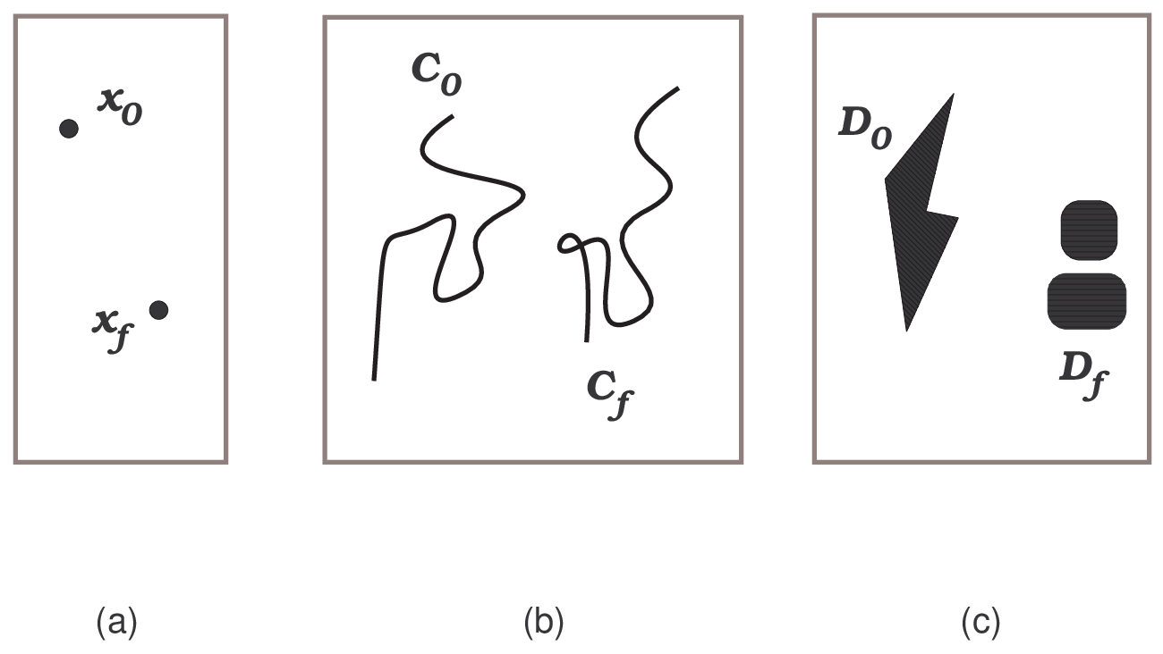
Refer to caption
Figure 2: Illustrative examples of the set SS used in the definition of Problem (𝑷)({\boldsymbol{P}}) given by Eq. (2).

The set SS in Problem (𝑷)({\boldsymbol{P}}) is quite arbitrary. In the simplest case of fixed points and fixed times (with the optimization parameter 𝒑{\boldsymbol{p}} fixed) SS is a singleton. Frequently, SS is a Cartesian product of two sets comprising an initial and final set. These aspects are illustrated in Fig. 2. In panel (a), the set SS is just (the Cartesian product of) two points. In panel (b), SS comprises curves denoted by C0C_{0} and CfC_{f} while panel (c) illustrates two nonconvex sets D0D_{0} and DfD_{f}.

Remark 1

Path constraints and functional constraints[6] may be incorporated in the definition of Problem (𝐏)({\boldsymbol{P}}). Because the main topic of this paper is transversality conditions, these additional constraints do not alter the results to follow. Hence, there is no loss in generality in omitting these constraints in the statement of Problem (𝐏)({\boldsymbol{P}}).

We assume all data functions in Problem (𝑷)({\boldsymbol{P}}) to be continuously differentiable with respect to all of their respective arguments. Hence, a statement of the necessary conditions for Problem (𝑷)({\boldsymbol{P}}) involves the structure and properties of the set SS. This topic constitutes the main discussion point of this section.

2.1 Mathematical Preliminaries

Because the endpoint condition in Problem (𝑷)({\boldsymbol{P}}) is defined in terms of an abstract set, it should not be a surprise that the transversality conditions are stated in terms of some property of SS. This property is called the normal cone[4, 13] and is defined in terms of a vector that “leaves SS orthogonally[13].” Although it is possible to define a normal cone independent of a tangent cone[4, 13], we take the simpler path of defining a tangent cone first. Fig. 3 provides a useful visual in understanding the definitions to follow.

Definition 1 (Tangent Cone[13, 16, 17])

A vector 𝐝χ{\boldsymbol{d}}_{\chi} is said to be a tangent vector to SS at the point 𝛘\chi if there is a sequence of feasible vectors {𝛘k}\left\{\mbox{\boldmath$\chi$}^{k}\right\} and a sequence of positive scalars {sk}\left\{s^{k}\right\} with sk→0s^{k}\to 0 such that

limk→∞𝝌k−𝝌sk=𝒅χ\lim_{k\to\infty}\frac{\mbox{\boldmath$\chi$}^{k}-\mbox{\boldmath$\chi$}}{s^{k}}={\boldsymbol{d}}_{\chi}

The set of all tangent vectors at 𝛘\chi, denoted by TS​(𝛘)T_{S}(\mbox{\boldmath$\chi$}), is called the tangent cone (to SS at 𝛘\chi).

Definition 2 (Normal Cone[4, 13, 16])

The normal cone to SS at a point 𝛘∈S\mbox{\boldmath$\chi$}\in S, denoted by NS​(𝛘)N_{S}(\mbox{\boldmath$\chi$}), is defined as,

NS​(𝝌):=limsupk→∞⁡TS∗​(𝝌k)N_{S}(\mbox{\boldmath$\chi$}):=\mathop{\lim\sup}_{k\to\infty}T_{S}^{*}(\mbox{\boldmath$\chi$}_{k})

where TS∗​(𝛘k)T_{S}^{*}(\mbox{\boldmath$\chi$}_{k}), called the polar cone to TS​(𝛘k)T_{S}(\mbox{\boldmath$\chi$}_{k}), is defined by,

TS∗(𝝌k):={𝜻χ:𝜻χT𝒅χ≤0∀𝒅χ∈TS(𝝌k)}T_{S}^{*}(\mbox{\boldmath$\chi$}_{k}):=\left\{\mbox{\boldmath$\zeta$}_{\chi}:\ \mbox{\boldmath$\zeta$}_{\chi}^{T}{\boldsymbol{d}}_{\chi}\leq 0\quad\forall\ {\boldsymbol{d}}_{\chi}\in T_{S}(\mbox{\boldmath$\chi$}_{k})\right\} (12)

A vector 𝛇χ∈NS​(𝛘)\mbox{\boldmath$\zeta$}_{\chi}\in N_{S}(\mbox{\boldmath$\chi$}) is called a normal vector to SS at 𝛘\chi.

Refer to caption
Figure 3: Tangent and normal vectors and cones at key points of a nonconvex set SS.

Fig. 3 illustrates all these cones at key points labeled AA, BB and CC:

  1. 1.

    Consider the point AA that lies on a smooth boundary of a set. Then the normal cone, NS​(A)N_{S}(A), is just the outward perpendicular to the tangent hyperplane. The tangent cone is the half-space indicated at the point AA in Fig. 3.

  2. 2.

    Consider the point BB that lies on a nonsmooth boundary point. This point is locally convex. In this case, the (convex) set of all outward normals is the normal cone NS​(B)N_{S}(B);

  3. 3.

    Consider the point CC on a nonsmooth boundary point that is not locally convex. In this case, the limiting set of all outward normals is the (nonconvex) normal cone NS​(C)N_{S}(C) that comprises just the two vectors shown in Fig. 3.

In the literature on nonsmooth calculus, a large number of tangent and normal cones are defined[4, 13, 19, 18]. The tangent cone of Definition 1 is called the Bouligand or contingent tangent cone[18, 13, 17] and the normal cone defined in Definition 2 is called the Mordukhovich or limiting normal cone[19, 13, 4]. In this paper, we will not use these qualifiers and rely exclusively on Definitions 1 and 2 because these cones are the most relevant to the formulation of transversality conditions.

Remark 2

In general, the tangent and normal cones are nonconvex; see the cones illustrated at the point CC in Fig. 3. Furthermore, note the following:

  1. 1.

    From their definitions, it is clear that zero is an element of both the tangent and normal cones. They are sketched in Fig. 3 as emanating from the point 𝛘\chi as a floating vector[20] instead of the origin[17] as in Fig. 4.

    Refer to caption
    Figure 4: Tangent and normal cones at the point BB of Fig. 3 and their different spaces.
  2. 2.

    The normal cone is a construct in dual space. The vector 𝜻χ\mbox{\boldmath$\zeta$}_{\chi} in Eq. (12) is a covector whose “units” are in “frequency”[6]. For example, the units of (χ1,χ2)(\chi_{1},\chi_{2}) and (ζ1,ζ2)(\zeta_{1},\zeta_{2}) in Fig. 4 are not the same. See [6] for details pertaining to a “physical interpretation” of covectors. The normal cone sketched in Fig. 3 uses the notion of a proxy vector to the covector[6] in order to display its connection to primal space.

  3. 3.

    Even though a vector and covector are elements in different vector spaces as shown in Fig. 4, we say 𝜻χ\mbox{\boldmath$\zeta$}_{\chi} is “orthogonal” to 𝒅χ{\boldsymbol{d}}_{\chi} if 𝜻χT​𝒅χ=0\mbox{\boldmath$\zeta$}_{\chi}^{T}{\boldsymbol{d}}_{\chi}=0. Note that each component of 𝜻χ\mbox{\boldmath$\zeta$}_{\chi} can have different units[6].

The transversality conditions for Problem (𝑷)({\boldsymbol{P}}) can be stated in terms of the following three constructs:

  1. (a)

    the endpoint values of the adjoint covector (costate),

  2. (b)

    the endpoint values of the lower (i.e., minimized) Hamiltonian, and

  3. (c)

    the normal cone to the set SS that defines the endpoint constraints.

To state these conditions we first write the (Pontryagin) Hamiltonian function for the pair (F,𝒇)(F,{\boldsymbol{f}}) as[6],

H⁡(𝝀,𝒙,𝒖,t,𝒑):=ν0​F​(𝒙,𝒖,t,𝒑)+𝝀T​𝒇​(𝒙,𝒖,t,𝒑)H({\mbox{\boldmath$\lambda$}},\boldsymbol{x},{\boldsymbol{u}},t,{\boldsymbol{p}}):=\nu^{0}\,F(\boldsymbol{x},{\boldsymbol{u}},t,{\boldsymbol{p}})+{\mbox{\boldmath$\lambda$}}^{T}{\boldsymbol{f}}(\boldsymbol{x},{\boldsymbol{u}},t,{\boldsymbol{p}}) (13)

where ν0≥0\nu^{0}\geq 0 is a cost multiplier and 𝝀∈ℝNx{\mbox{\boldmath$\lambda$}}\in{\mathbb{R}}^{N_{x}} is a covector that satisfies the adjoint differential equation,

−𝝀˙​(t)=∂𝒙H⁡(𝝀⁡(t),𝒙⁡(t),𝒖⁡(t),t,𝒑)-\dot{\mbox{\boldmath$\lambda$}}(t)=\partial_{\boldsymbol{x}}H({\mbox{\boldmath$\lambda$}}(t),\boldsymbol{x}(t),{\boldsymbol{u}}(t),t,{\boldsymbol{p}}) (14)

Typically, we have ν0>0\nu^{0}>0, the so-called normal case[6]. If ν0=0\nu^{0}=0 the case is deemed “abnormal.” In the normal case, we may use ν0>0\nu^{0}>0 to scale and balance the adjoint equations[21] in a computational setting or simply set ν0=1\nu^{0}=1 for theoretical analysis. The centerpiece of Pontryagin’s Principle is the Hamiltonian Minimization Condition (HMC), a static, time-varying, instantaneous optimization problem, defined by[6]:

(H​M​C)​{​M​i​n​i​m​i​z​e𝒖⁡(t)H⁡(𝝀⁡(t),𝒙⁡(t),𝒖⁡(t),t,𝒑)​S​u​b​j​e​c​t​t​o𝒖⁡(t)∈U⁡(t)\displaystyle(\textsf{$HMC$})\left\{\begin{array}[]{lll}\displaystyle\mathop{\emph{Minimize}}_{{\boldsymbol{u}}(t)}&H({\mbox{\boldmath$\lambda$}}(t),\boldsymbol{x}(t),{\boldsymbol{u}}(t),t,{\boldsymbol{p}})\\[5.0pt] \emph{Subjectto}&{\boldsymbol{u}}(t)\in U(t)\end{array}\right.

A (conceptual) solution to Problem (H​M​C)(HMC) is given by,

𝒖∗​(𝝀⁡(t),𝒙⁡(t),t,𝒑)=arg⁡min𝒖⁡(t)∈U⁡(t)⁡H⁡(𝝀⁡(t),𝒙⁡(t),𝒖⁡(t),t,𝒑){\boldsymbol{u}}^{*}({\mbox{\boldmath$\lambda$}}(t),\boldsymbol{x}(t),t,{\boldsymbol{p}})=\arg\min_{{\boldsymbol{u}}(t)\in U(t)}H({\mbox{\boldmath$\lambda$}}(t),\boldsymbol{x}(t),{\boldsymbol{u}}(t),t,{\boldsymbol{p}}) (18)

Substituting Eq. (18) in Eq. (13) eliminates 𝒖{\boldsymbol{u}} and generates the lower Hamiltonian[6, 13],

ℋ⁡(𝝀⁡(t),𝒙⁡(t),t,𝒑)=H⁡(𝝀⁡(t),𝒙,𝒖∗​(𝝀⁡(t),𝒙⁡(t),t,𝒑),t,𝒑)\mathcal{H}({\mbox{\boldmath$\lambda$}}(t),\boldsymbol{x}(t),t,{\boldsymbol{p}})=H({\mbox{\boldmath$\lambda$}}(t),\boldsymbol{x},{\boldsymbol{u}}^{*}({\mbox{\boldmath$\lambda$}}(t),\boldsymbol{x}(t),t,{\boldsymbol{p}}),t,{\boldsymbol{p}}) (19)

Note that the lower Hamiltonian ℋ\mathcal{H} is not a function of the control variable. It is frequently nondifferentiable[6].

In the discussions to follow, it will be convenient to use the following abbreviation:

𝒙(t0)≡𝒙0,𝒙(tf)≡𝒙f,andℋ(𝝀(t),𝒙(t),t,𝒑)≡ℋ[@t]\boldsymbol{x}(t_{0})\equiv\boldsymbol{x}_{0},\quad\quad\boldsymbol{x}(t_{f})\equiv\boldsymbol{x}_{f},\quad{and}\quad\mathcal{H}({\mbox{\boldmath$\lambda$}}(t),\boldsymbol{x}(t),t,{\boldsymbol{p}})\equiv\mathcal{H}[@t] (20)

2.2 Transversality Conditions for the Case When 𝒑{\boldsymbol{p}} is Not an Optimization Variable

Much of the literature contains necessary conditions for the case when 𝒑{\boldsymbol{p}} is not an optimization variable. Hence, the case when 𝒑{\boldsymbol{p}} is indeed an optimization variable deserves special consideration. This case is deferred to the next subsection.

Theorem 1 ([13, 4])

Let Problem (𝐏♯{\boldsymbol{P}}^{\sharp}) denote the special case of Problem (𝐏)({\boldsymbol{P}}) when 𝐩{\boldsymbol{p}} is fixed to a given value 𝐩=𝐩♯{\boldsymbol{p}}={\boldsymbol{p}}^{\sharp}. Let ℋ⁡[@​t]\mathcal{H}[@t] denote an abbreviated notation for ℋ⁡(𝛌⁡(t),𝐱⁡(t),t,𝐩♯)\mathcal{H}({\mbox{\boldmath$\lambda$}}(t),\boldsymbol{x}(t),t,{\boldsymbol{p}}^{\sharp}). Then the transversality condition for Problem (𝐏♯{\boldsymbol{P}}^{\sharp}) is given by,

(−𝝀⁡(t0),ℋ⁡[@​t0],𝝀⁡(tf),−ℋ⁡[@​tf])∈ν0​∂(𝒙0,t0,𝒙f,tf)E⁡(𝒙0,t0,𝒙f,tf,𝒑♯)+NS​(𝒙0,t0,𝒙f,tf,𝒑♯)\big(-{\mbox{\boldmath$\lambda$}}(t_{0}),\mathcal{H}[@t_{0}],{\mbox{\boldmath$\lambda$}}(t_{f}),-\mathcal{H}[@t_{f}]\big)\in\nu^{0}\,\partial_{(\boldsymbol{x}_{0},t_{0},\boldsymbol{x}_{f},t_{f})}E(\boldsymbol{x}_{0},t_{0},\boldsymbol{x}_{f},t_{f},{\boldsymbol{p}}^{\sharp})+N_{S}(\boldsymbol{x}_{0},t_{0},\boldsymbol{x}_{f},t_{f};{\boldsymbol{p}}^{\sharp}) (21)

where 𝐱0\boldsymbol{x}_{0} and 𝐱f\boldsymbol{x}_{f} are 𝐱⁡(t0)\boldsymbol{x}(t_{0}) and 𝐱⁡(tf)\boldsymbol{x}(t_{f}) as respectively in accordance with Eq. (20).

Theorem 1 is an elegant statement of transversality conditions cast in geometric terms. However, for Eq. (21) to be useful from a computational perspective, it requires a mechanism to compute NSN_{S}. To clarify this statement, we first rewrite Eq. (21) in a more convenient “equality” form as,

(−𝝀⁡(t0),ℋ⁡[@​t0],𝝀⁡(tf),−ℋ⁡[@​tf])=ν0​∂(𝒙0,t0,𝒙f,tf)E⁡(𝒙0,t0,𝒙f,tf,𝒑♯)+𝜼\big(-{\mbox{\boldmath$\lambda$}}(t_{0}),\mathcal{H}[@t_{0}],{\mbox{\boldmath$\lambda$}}(t_{f}),-\mathcal{H}[@t_{f}]\big)=\nu^{0}\,\partial_{(\boldsymbol{x}_{0},t_{0},\boldsymbol{x}_{f},t_{f})}E(\boldsymbol{x}_{0},t_{0},\boldsymbol{x}_{f},t_{f},{\boldsymbol{p}}^{\sharp})+\mbox{\boldmath$\eta$} (22)

for some 𝜼∈NS​(𝒙0,t0,𝒙f,tf,𝒑♯)\mbox{\boldmath$\eta$}\in N_{S}(\boldsymbol{x}_{0},t_{0},\boldsymbol{x}_{f},t_{f},{\boldsymbol{p}}^{\sharp}). Equation (22) reveals that the main problem in computing the transversality condition is centered around finding a suitable 𝜼\eta.

As powerful as it is, it turns out Theorem 1 is not sufficient to handle the production of transversality conditions for the motivating problems illustrated in Fig. 1. In fact, what is needed is an inclusion of the case when 𝒑{\boldsymbol{p}} is an optimization variable.

2.3 Transversality Conditions for the General Case

The general case when 𝒑{\boldsymbol{p}} is an optimization variable deserves special attention due to an unfortunate error in the original work by Pontryagin et al[14]. This error in the necessary optimality condition for 𝒑{\boldsymbol{p}} was first noted and corrected by Hofer and Sagirow in 1968[22]. The corrected necessary condition was subsequently generalized by other authors[23, 24, 25]. In principle, the necessary condition for an optimal 𝒑{\boldsymbol{p}} is not part of the transversality condition; however, because 𝒑{\boldsymbol{p}} appears in the endpoint functional and constraints (see Eq. (2)) it cannot be decoupled in the computation of the normal cone in Eq. (21) (or Eq. (22)). As noted earlier, we will utilize the general case in Section 5.

To combine the result of Theorem 1 with the results of [22, 23, 24, 25] we define a quantity 𝝈∈ℝNp\mbox{\boldmath$\sigma$}\in{\mathbb{R}}^{N_{p}} according to,

𝝈:=∫t0tf∂𝒑H⁡(𝝀⁡(t),𝒙⁡(t),𝒖⁡(t),t,𝒑)​𝑑t\mbox{\boldmath$\sigma$}:=\int_{t_{0}}^{t_{f}}\partial_{\boldsymbol{p}}H({\mbox{\boldmath$\lambda$}}(t),\boldsymbol{x}(t),{\boldsymbol{u}}(t),t,{\boldsymbol{p}})\,dt (23)

If 𝒑{\boldsymbol{p}} is unconstrained, then the “corrected” necessary condition[22, 23, 24, 25] for optimality is given by,

−𝝈=ν0​∂𝒑E⁡(𝒙0,t0,𝒙f,tf,𝒑)-\mbox{\boldmath$\sigma$}=\nu^{0}\,\partial_{\boldsymbol{p}}E(\boldsymbol{x}_{0},t_{0},\boldsymbol{x}_{f},t_{f},{\boldsymbol{p}}) (24)

If 𝒑{\boldsymbol{p}} is constrained then 𝝈+ν0​∂𝒑E⁡(𝒙0,t0,𝒙f,tf,𝒑)\mbox{\boldmath$\sigma$}+\nu^{0}\,\partial_{\boldsymbol{p}}E(\boldsymbol{x}_{0},t_{0},\boldsymbol{x}_{f},t_{f},{\boldsymbol{p}}) satisfies necessary conditions[23, 24, 25] given by the Karush-Kuhn-Tucker (KKT) theorem[16]. In view of this result, Theorem 1 generalizes accordingly and can be stated as follows:

Theorem 2

The transversality condition for Problem (𝐏{\boldsymbol{P}}) is given by,

(−𝝀⁡(t0),ℋ⁡[@​t0],𝝀⁡(tf),−ℋ⁡[@​tf],−𝝈)∈ν0​∂(𝒙0,t0,𝒙f,tf,𝒑)E⁡(𝒙0,t0,𝒙f,tf,𝒑)+NS​(𝒙0,t0,𝒙f,tf,𝒑)\big(-{\mbox{\boldmath$\lambda$}}(t_{0}),\mathcal{H}[@t_{0}],{\mbox{\boldmath$\lambda$}}(t_{f}),-\mathcal{H}[@t_{f}],-\mbox{\boldmath$\sigma$}\big)\in\nu^{0}\,\partial_{(\boldsymbol{x}_{0},t_{0},\boldsymbol{x}_{f},t_{f},{\boldsymbol{p}})}E(\boldsymbol{x}_{0},t_{0},\boldsymbol{x}_{f},t_{f},{\boldsymbol{p}})+N_{S}(\boldsymbol{x}_{0},t_{0},\boldsymbol{x}_{f},t_{f},{\boldsymbol{p}}) (25)

or equivalently as,

(−𝝀⁡(t0),ℋ⁡[@​t0],𝝀⁡(tf),−ℋ⁡[@​tf],−𝝈)=ν0​∂(𝒙0,t0,𝒙f,tf,𝒑)E⁡(𝒙0,t0,𝒙f,tf,𝒑)+𝜼\big(-{\mbox{\boldmath$\lambda$}}(t_{0}),\mathcal{H}[@t_{0}],{\mbox{\boldmath$\lambda$}}(t_{f}),-\mathcal{H}[@t_{f}],-\mbox{\boldmath$\sigma$}\big)=\nu^{0}\,\partial_{(\boldsymbol{x}_{0},t_{0},\boldsymbol{x}_{f},t_{f},{\boldsymbol{p}})}E(\boldsymbol{x}_{0},t_{0},\boldsymbol{x}_{f},t_{f},{\boldsymbol{p}})+\mbox{\boldmath$\eta$} (26)

where 𝛈∈NS​(𝐱0,t0,𝐱f,tf,𝐩)\mbox{\boldmath$\eta$}\in N_{S}(\boldsymbol{x}_{0},t_{0},\boldsymbol{x}_{f},t_{f},{\boldsymbol{p}}) and 𝐱0\boldsymbol{x}_{0}, 𝐱f\boldsymbol{x}_{f}, ℋ⁡[@​t0]\mathcal{H}[@t_{0}] and ℋ⁡[@​tf]\mathcal{H}[@t_{f}] denote 𝐱⁡(t0)\boldsymbol{x}(t_{0}), 𝐱⁡(tf)\boldsymbol{x}(t_{f}), ℋ⁡(𝛌⁡(t0),𝐱⁡(t0),t0,𝐩)\mathcal{H}({\mbox{\boldmath$\lambda$}}(t_{0}),\boldsymbol{x}(t_{0}),t_{0},{\boldsymbol{p}}), and ℋ⁡(𝛌⁡(tf),𝐱⁡(tf),tf,𝐩)\mathcal{H}({\mbox{\boldmath$\lambda$}}(t_{f}),\boldsymbol{x}(t_{f}),t_{f},{\boldsymbol{p}}) respectively.

In the sections to follow, we will use Theorem 2 as our building block to formulate new computable transversality conditions.

2.4 Transversality Conditions When SS Is Parameterized by Algebraic Inequalities

The most common “application” of Theorem 2 (and hence Theorem 1) is when the set SS is parameterized by algebraic inequalities,

S=Sa​l​g:={(𝒙0,t0,𝒙f,tf,𝒑):𝒆L≤𝒆⁡(𝒙0,t0,𝒙f,tf,𝒑)≤𝒆U}S=S^{alg}:=\left\{(\boldsymbol{x}_{0},t_{0},\boldsymbol{x}_{f},t_{f},{\boldsymbol{p}}):\ {\boldsymbol{e}}^{L}\leq{\boldsymbol{e}}(\boldsymbol{x}_{0},t_{0},\boldsymbol{x}_{f},t_{f},{\boldsymbol{p}})\leq{\boldsymbol{e}}^{U}\right\} (27)

where 𝒆:(𝒙0,t0,𝒙f,tf,𝒑)↦ℝNe{\boldsymbol{e}}:(\boldsymbol{x}_{0},t_{0},\boldsymbol{x}_{f},t_{f},{\boldsymbol{p}})\mapsto{\mathbb{R}}^{N_{e}} is a continuously differentiable (“algebraic”) function, 𝒆L∈ℝNe{\boldsymbol{e}}^{L}\in{\mathbb{R}}^{N_{e}} is a lower bound on the allowable values of 𝒆{\boldsymbol{e}} and 𝒆U≥𝒆L{\boldsymbol{e}}^{U}\geq{\boldsymbol{e}}^{L} is the corresponding upper bound. A large class of practical optimal control problems (barring the ones identified in Section 1) have boundary conditions that are conveniently described in the form given by Eq. (27). Then, it can be shown[4, 13] that Theorem 2 reduces to the transversality conditions given by the following familiar theorem[6]:

Theorem 3

Let Problem (𝐏a​l​g{\boldsymbol{P}}^{alg}) denote the special case of Problem (𝐏)({\boldsymbol{P}}) where the boundary condition is defined by Sa​l​gS^{alg} given by Eq. (27). Then the transversality conditions for Problem (𝐏a​l​g)({\boldsymbol{P}}^{alg}) together with the necessary condition for optimal 𝐩{\boldsymbol{p}} are given by,

−𝝀⁡(t0)\displaystyle-{\mbox{\boldmath$\lambda$}}(t_{0}) =∂𝒙0E¯​(𝝂,𝒙0,t0,𝒙f,tf,𝒑)\displaystyle=\partial_{\boldsymbol{x}_{0}}\overline{E}({\mbox{\boldmath$\nu$}},\boldsymbol{x}_{0},t_{0},\boldsymbol{x}_{f},t_{f},{\boldsymbol{p}}) (28a)
ℋ⁡[@​t0]\displaystyle\mathcal{H}[@t_{0}] =∂t0E¯​(𝝂,𝒙0,t0,𝒙f,tf,𝒑)\displaystyle=\partial_{t_{0}}\overline{E}({\mbox{\boldmath$\nu$}},\boldsymbol{x}_{0},t_{0},\boldsymbol{x}_{f},t_{f},{\boldsymbol{p}}) (28b)
𝝀⁡(tf)\displaystyle{\mbox{\boldmath$\lambda$}}(t_{f}) =∂𝒙fE¯​(𝝂,𝒙0,t0,𝒙f,tf,𝒑)\displaystyle=\partial_{\boldsymbol{x}_{f}}\overline{E}({\mbox{\boldmath$\nu$}},\boldsymbol{x}_{0},t_{0},\boldsymbol{x}_{f},t_{f},{\boldsymbol{p}}) (28c)
−ℋ⁡[@​tf]\displaystyle-\mathcal{H}[@t_{f}] =∂tfE¯​(𝝂,𝒙0,t0,𝒙f,tf,𝒑)\displaystyle=\partial_{t_{f}}\overline{E}({\mbox{\boldmath$\nu$}},\boldsymbol{x}_{0},t_{0},\boldsymbol{x}_{f},t_{f},{\boldsymbol{p}}) (28d)
−𝝈\displaystyle-\mbox{\boldmath$\sigma$} =∂𝒑E¯​(𝝂,𝒙0,t0,𝒙f,tf,𝒑)\displaystyle=\partial_{{\boldsymbol{p}}}\overline{E}({\mbox{\boldmath$\nu$}},\boldsymbol{x}_{0},t_{0},\boldsymbol{x}_{f},t_{f},{\boldsymbol{p}}) (28e)

where E¯\overline{E} is the endpoint Lagrangian[6] defined by,

E¯​(𝝂,𝒙0,t0,𝒙f,tf,𝒑):=ν0​E​(𝒙0,t0,𝒙f,tf,𝒑)+𝝂T​𝒆​(𝒙0,t0,𝒙f,tf,𝒑)\overline{E}({\mbox{\boldmath$\nu$}},\boldsymbol{x}_{0},t_{0},\boldsymbol{x}_{f},t_{f},{\boldsymbol{p}}):=\nu^{0}\,E(\boldsymbol{x}_{0},t_{0},\boldsymbol{x}_{f},t_{f},{\boldsymbol{p}})+{\mbox{\boldmath$\nu$}}^{T}{\boldsymbol{e}}(\boldsymbol{x}_{0},t_{0},\boldsymbol{x}_{f},t_{f},{\boldsymbol{p}}) (29)

and 𝛎∈ℝNe{\mbox{\boldmath$\nu$}}\in{\mathbb{R}}^{N_{e}} is an endpoint covector that satisfies the following complementarity conditions[6],

𝝂†𝒆⁡(𝒙0,t0,𝒙f,tf,𝒑)⇔νi​{≤0,if ​ei​(𝒙0,t0,𝒙f,tf,𝒑)=eiL=0,if ​eiL<ei​(𝒙0,t0,𝒙f,tf,𝒑)<eiU≥0,if ​ei​(𝒙0,t0,𝒙f,tf,𝒑)=eiUany value,if ​eiL=eiU\displaystyle{\mbox{\boldmath$\nu$}}\dagger{\boldsymbol{e}}(\boldsymbol{x}_{0},t_{0},\boldsymbol{x}_{f},t_{f},{\boldsymbol{p}})\Leftrightarrow\nu_{i}\left\{\begin{array}[]{ll}\leq 0,&\hbox{\text{if} }\ e_{i}(\boldsymbol{x}_{0},t_{0},\boldsymbol{x}_{f},t_{f},{\boldsymbol{p}})=e_{i}^{L}\\ =0,&\hbox{if }\ e_{i}^{L}<e_{i}(\boldsymbol{x}_{0},t_{0},\boldsymbol{x}_{f},t_{f},{\boldsymbol{p}})<e_{i}^{U}\\ \geq 0,&\hbox{if }\ e_{i}(\boldsymbol{x}_{0},t_{0},\boldsymbol{x}_{f},t_{f},{\boldsymbol{p}})=e_{i}^{U}\\ \text{any value},&\hbox{if }\ e_{i}^{L}=e_{i}^{U}\end{array}\right.
Remark 3

Comparing Eq. (28) with Eq. (26) it follows that 𝛈\eta (i.e., a vector in the normal cone; see Definition 2) encapsulates, in one fell swoop, the combined notion of complementarity conditions (see Eq. (3)) and the idea of expressing a vector as a linear combination of the active gradients of the individual endpoint constraint functions ei​(𝐱0,t0,𝐱f,tf,𝐩),i=1,…,Nee_{i}(\boldsymbol{x}_{0},t_{0},\boldsymbol{x}_{f},t_{f},{\boldsymbol{p}}),\ i=1,\ldots,N_{e} according to the following:

𝜼∈NSa​l​g:={𝝃∈ℝNx×ℝ×ℝNx×ℝ×ℝNp:𝝃=[∂(𝒙0,t0,𝒙f,tf,𝒑)𝒆(𝒙0,t0,𝒙f,tf,𝒑)]T𝝂,𝝂†𝒆(𝒙0,t0,𝒙f,tf,𝒑)}\mbox{\boldmath$\eta$}\in N_{S^{alg}}:=\left\{{\mbox{\boldmath$\xi$}}\in{\mathbb{R}}^{N_{x}}\times\mathbb{R}\times{\mathbb{R}}^{N_{x}}\times\mathbb{R}\times{\mathbb{R}}^{N_{p}}:\ \right.\\ \left.{\mbox{\boldmath$\xi$}}=\big[\partial_{(\boldsymbol{x}_{0},t_{0},\boldsymbol{x}_{f},t_{f},{\boldsymbol{p}})}{\boldsymbol{e}}(\boldsymbol{x}_{0},t_{0},\boldsymbol{x}_{f},t_{f},{\boldsymbol{p}})\big]^{T}{\mbox{\boldmath$\nu$}},\ {\mbox{\boldmath$\nu$}}\dagger{\boldsymbol{e}}(\boldsymbol{x}_{0},t_{0},\boldsymbol{x}_{f},t_{f},{\boldsymbol{p}})\right\} (34)
Remark 4

If the endpoint constraint function is given by a box constraint, then 𝛏\xi in Eq. (34) reduces to 𝛎\nu. In this case, 𝛎\nu can be visualized as a vector in the normal cone to a point in a box as illustrated in Fig. 5. Hence, when we encounter this special case, we may use the symbols 𝛈\eta and 𝛎\nu interchangeably.

Refer to caption
Figure 5: Normal cones and vectors at various points on a box constraint.

Theorem 3 is the computational version of Theorem 2 for the special case of S=Sa​l​gS=S^{alg} where Sa​l​gS^{alg} is given in terms of algebraic equations. Although Theorem 3 is presented in this section as a special case of Theorem 2, the latter is a generalization of the former from a historical perspective[23, 25].

Remark 5

As noted in the statement of Theorem 3, Eq. (28e) is technically not a transversality condition. Nonetheless, it is apparent that Eq. (28e) is integral to the transversality conditions as it helps determine 𝐩{\boldsymbol{p}}. Furthermore, because the necessary condition for 𝐩{\boldsymbol{p}} cannot be separated, in general, from the broader transversality condition (see Eq. (25) and Eq. (26)) we group it with Eq. (28).

Remark 6

If the Hamiltonian does not depend upon 𝐩{\boldsymbol{p}}, then 𝛔=𝟎\mbox{\boldmath$\sigma$}={\bf 0}; see Eq. (23). Then Eq. (28e) reduces to the familiar KKT conditions[16] for parameter optimization. As an interesting side note, the connection between transversality conditions and the KKT conditions has been utilized in [27, 29, 28, 26] to construct an optimal control theory for optimization.

3 Foundations of Boundary Conditions Defined by Differential Equations

The transversality conditions that are of main interest in this paper are those conditions when SS is given by So​d​e+S^{ode+}, an endpoint set defined by differential equations with side conditions. To better understand what we mean by “differential equations with side conditions,” it is instructive to develop a definition of So​d​e+S^{ode+} in stages of increasing intricacies rather than all at once.

3.1 A Basic Set Parameterized by a Differential Equation

Consider an initial-value problem (IVP) corresponding to a non-autonomous differential equation given by,

d​𝒙d​s:=𝒙′=𝒈⁡(𝒙,s),𝒙⁡(s♯)=𝒙♯\frac{d\boldsymbol{x}}{ds}:=\boldsymbol{x}^{\prime}={\boldsymbol{g}}(\boldsymbol{x},s),\quad\boldsymbol{x}(s^{\sharp})=\boldsymbol{x}^{\sharp} (35)

where (𝒙♯,s♯)∈ℝNx×ℝ(\boldsymbol{x}^{\sharp},s^{\sharp})\in{\mathbb{R}}^{N_{x}}\times\mathbb{R} is a given point in “space” and “time.” We choose the symbol ss for the independent variable instead of tt in order to reserve the latter notation for the clock time implied in Section 2. The distinctions between ss and tt will become more apparent in the discussion to follow. Where convenient, we will refer to ss as ss-time or local ss-time.

If the function 𝒈{\boldsymbol{g}} satisfies the conditions of the Picard-Lindelöf theorem[30, 31], then there is a unique solution to Eq. (35) that passes through the point (𝒙♯,s♯)(\boldsymbol{x}^{\sharp},s^{\sharp}); see Fig. 6.

Refer to caption
Figure 6: Schematic of a “curve” corresponding to Eq. (35).

This solution can be described as the set of all points in ℝNx×ℝ{\mathbb{R}}^{N_{x}}\times\mathbb{R} that satisfies Eq. (35). This set is a “curve” parameterized by ss and can be written as a “point-to-set” map:

C(𝒙♯,s♯):={(𝒙(s),s)∈ℝNx×ℝ:𝒙′(s)=𝒈(𝒙(s),s),𝒙(s♯)=𝒙♯}C(\boldsymbol{x}^{\sharp},s^{\sharp}):=\left\{(\boldsymbol{x}(s),s)\in{\mathbb{R}}^{N_{x}}\times\mathbb{R}:\ \boldsymbol{x}^{\prime}(s)={\boldsymbol{g}}(\boldsymbol{x}(s),s),\quad\boldsymbol{x}(s^{\sharp})=\boldsymbol{x}^{\sharp}\right\} (36)

The notation C⁡(𝒙♯,s♯)C(\boldsymbol{x}^{\sharp},s^{\sharp}) implies a point (𝒙♯,s♯)(\boldsymbol{x}^{\sharp},s^{\sharp}) must be given (i.e., a side condition) to construct the set defined in the right hand side of Eq. (36).

Remark 7

Fig. 6 and Eq. (36) appear to suggest that the solution to Eq. (35) is valid for infinite ss-time forwards and backwards; i.e., s∈(−∞,∞)s\in(-\infty,\infty). This strong assumption is only tentative. We can easily add bounds to the independent variable, ss, according to sL≤s≤sUs^{L}\leq s\leq s^{U}, where sL<sU∈ℝs^{L}<s^{U}\in\mathbb{R}. Furthermore, we may easily incorporate additional rules to sLs^{L} and sUs^{U} such as dependencies on (𝐱♯,s♯)(\boldsymbol{x}^{\sharp},s^{\sharp}) as done in typical textbooks on differential equations[31, 30]. In order to construct the ideas piecemeal, we ignore such technicalities in favor of clarity.

From Remark 7 it follows that Eq. (36) is not sufficient to define So​d​eS^{ode}. We need one or more side conditions in order to fortify a definition of an endpoint set given by differential equations.

3.2 A Manifold Parameterized by Differential Equations

Now consider another set P⊂ℝNx×ℝP\subset{\mathbb{R}}^{N_{x}}\times\mathbb{R} from where we pick different initial conditions (𝒙♯,s♯)∈P(\boldsymbol{x}^{\sharp},s^{\sharp})\in P. That is, consider now a new set that generalizes Eq. (36) as follows:

M:={(𝒙⁡(s),s)∈C⁡(𝒙♯,s♯),(𝒙♯,s♯)∈P}:={(𝒙(s),s,𝒙♯,s♯)∈(ℝNx×ℝ)×P:𝒙′(s)=𝒈(𝒙(s),s),𝒙(s♯)=𝒙♯}M:=\left\{(\boldsymbol{x}(s),s)\in C(\boldsymbol{x}^{\sharp},s^{\sharp}),(\boldsymbol{x}^{\sharp},s^{\sharp})\in P\right\}\\ :=\left\{(\boldsymbol{x}(s),s,\boldsymbol{x}^{\sharp},s^{\sharp})\in\left({\mathbb{R}}^{N_{x}}\times\mathbb{R}\right)\times P:\ \boldsymbol{x}^{\prime}(s)={\boldsymbol{g}}(\boldsymbol{x}(s),s),\quad\boldsymbol{x}(s^{\sharp})=\boldsymbol{x}^{\sharp}\right\} (37)

The construction of MM is as follows: Pick a point (𝒙♯,s♯)∈P(\boldsymbol{x}^{\sharp},s^{\sharp})\in P and construct C⁡(𝒙♯,s♯)C(\boldsymbol{x}^{\sharp},s^{\sharp}) according to Eq. (36). Pick a different point (𝒙♯,s♯)∈P(\boldsymbol{x}^{\sharp},s^{\sharp})\in P and repeat the process as illustrated in Fig. 7.

Refer to caption
Figure 7: Schematic illustrating Eq. (37) as a model for a manifold described by an ODE.

By arguments similar to those of the previous paragraphs, we now have solutions passing through each point in PP. Fig. 7 illustrates these ideas as well as a particular rendition of Eq. (37). In this illustration, M⊃C⁡(𝒙♯,s♯)M\supset C(\boldsymbol{x}^{\sharp},s^{\sharp}). Note also that MM is not necessarily the same as PP as illustrated in Fig. 7. Typically, PP is contained in MM. In Eq. (37), PP is a side condition. The set of points (𝒙♯,s♯)∈P(\boldsymbol{x}^{\sharp},s^{\sharp})\in P are the initial condition for Eq. (35). These points do not constitute nor limit the candidate initial conditions (𝒙0,t0)(\boldsymbol{x}_{0},t_{0}) to the set PP. To sharpen these distinctions, we call (𝒙♯,s♯)(\boldsymbol{x}^{\sharp},s^{\sharp}) the phantom initial conditions.

Definition 3 (phantom initial conditions)

The set of points (𝐱♯,s♯)∈P(\boldsymbol{x}^{\sharp},s^{\sharp})\in P that generate the flow of the ODE 𝐱′​(s)=𝐠⁡(𝐱⁡(s),s)\boldsymbol{x}^{\prime}(s)={\boldsymbol{g}}(\boldsymbol{x}(s),s) are called the phantom initial conditions.

Although MM generalizes CC, it is not yet complete to describe our first goal of defining So​d​e+S^{ode+}. To further a definition of So​d​e+S^{ode+}, we need a mechanism to connect the local ss-time with the transfer tt-time. To produce this connection, we develop the concept of coordinated and uncoordinated clock times.

3.3 Coordinated and Uncoordinated Clock Times

Consider the mathematical problem of defining an initial point (𝒙0,t0)(\boldsymbol{x}_{0},t_{0}) (of an optimal control problem) in terms of differential equations. As indicated earlier, the ss-time in Eq. (35) and the tt-time in Section 2 are not necessarily the same. The following example amplifies this point.

Example 1

Suppose 𝐱=(x,y)∈ℝ2\boldsymbol{x}=(x,y)\in{\mathbb{R}}^{2} and we require 𝐱0=𝐱⁡(t0)\boldsymbol{x}_{0}=\boldsymbol{x}(t_{0}) in an optimal control problem to be selected from a unit circle so that the initial conditions are required to satisfy the constraint, x02+y02=1x^{2}_{0}+y^{2}_{0}=1. See Fig. 8. This circle can also be parameterized as x0​(t)=sin⁡(t)x_{0}(t)=\sin(t) and y0​(t)=cos⁡(t)y_{0}(t)=\cos(t). Obviously, tt in this parametrization has no bearing on the clock time tt (or t0t_{0}).

Refer to caption
Figure 8: Two different parameterizations of a 11-dimensional manifold.

In the case of Example 1 when tt is not the same as the clock time, the unit circle is parameterized as (sin⁡(s),cos⁡(s))(\sin(s),\cos(s)) instead of (sin⁡(t),cos⁡(t))(\sin(t),\cos(t)). Using the symbol ss instead of tt addresses the problem of keeping ss and tt distinct; however, it requires a few caveats and some additional clarity in notation. To understand this point, suppose we write,

x0​(s)=sin⁡(s),y0​(s)=cos⁡(s)x_{0}(s)=\sin(s),\quad y_{0}(s)=\cos(s) (38)

Then substituting s=t0s=t_{0} in Eq. (38) generates x0​(t0)=sin⁡(t0),y0​(t0)=cos⁡(t0)x_{0}(t_{0})=\sin(t_{0}),y_{0}(t_{0})=\cos(t_{0}) which might (incorrectly) be construed to imply that the only valid value of the initial conditions is at s=t0s=t_{0}. But note, however, the symbolic difference between x0​(t0)x_{0}(t_{0}) and x⁡(t0)x(t_{0}). Per Eq. (20), x⁡(t0)x(t_{0}) is just x0x_{0}. The symbol x0​(t0)x_{0}(t_{0}) represents an allowable value of x0x_{0} at s=t0s=t_{0} when it is parameterized as x0​(s)x_{0}(s). That is, x0​(s)x_{0}(s) is a new symbol that represents all allowable values of x0=x⁡(t0)x_{0}=x(t_{0}). Because x0x_{0} itself is parameterized by ss-time, we use the symbol (x0,y0)(x_{0},y_{0}) (resp. (xf,yf)(x_{f},y_{f})) without its argument t0t_{0} (resp. tft_{f}) to rewrite Eq. (38) as,

x0=x0​(s)(:=sin⁡(s)),y0=y0​(s)(:=cos⁡(s))x_{0}=x_{0}(s)\Big(:=\sin(s)\Big),\quad y_{0}=y_{0}(s)\Big(:=\cos(s)\Big) (39)

In other words, the symbol 𝒙0\boldsymbol{x}_{0} implies 𝒙⁡(t0)\boldsymbol{x}(t_{0}) as always but 𝒙0​(s)\boldsymbol{x}_{0}(s) implies a parametrization of 𝒙0\boldsymbol{x}_{0} (via the independent variable ss). Hence, in Eq. (39) ss can take any value via the notation x0​(s)x_{0}(s) and y0​(s)y_{0}(s); and, no matter the value of ss, the outputs of x0​(s)x_{0}(s) and y0​(s)y_{0}(s), denoted by x0x_{0} and y0y_{0} respectively, remains on the unit circle.

Remark 8

Equation (39) suggests that it might be more prudent to use a different symbol (other than x0​(s),y0​(s)x_{0}(s),y_{0}(s)) for the right-hand-side of the equalities. Although such notational change might add clarity for this specific purpose, it also has the effect of obscuring the meaning of prior equations (and the ones to follow). For instance, if the symbol 𝐱\boldsymbol{x} was not used in Eq. (35) as a means to add extra clarity to Eq. (39), then, the IVP would read,

d​𝒚d​s:=𝒚′=𝒈⁡(𝒚,s),𝒚⁡(s♯)=𝒙♯\frac{d{\boldsymbol{y}}}{ds}:={\boldsymbol{y}}^{\prime}={\boldsymbol{g}}({\boldsymbol{y}},s),\quad{\boldsymbol{y}}(s^{\sharp})=\boldsymbol{x}^{\sharp}

with the understanding that 𝐲{\boldsymbol{y}} is a proxy for 𝐱0\boldsymbol{x}_{0}.

Returning to the problem at hand, it is also possible to construct optimal control problems wherein ss and tt are indeed coordinated clock times. Practical examples of such problems are those pertaining to intercept and rendezvous[3, 5, 6]. In the case of Example 1 for instance, it is quite possible that the unit circle may indeed be generated by a physical system going around in a circle. In this situation, the ss-clock time will certainly matter (mod 2​π2\pi). To allow for both possibilities, namely, ss and tt being coordinated or uncoordinated, we define the following:

Definition 4 (Coordinated and Uncoordinated Clock Times)

Let ϕ:ℝ×ℝ→ℝ\phi:\mathbb{R}\times\mathbb{R}\to\mathbb{R} be a continuously differentiable function of its arguments such that ϕ⁡(s,t)=0\phi(s,t)=0 has a real-valued unique solution for ss in terms of tt and vice versa. If ϕ≢0\phi\not\equiv 0, then we say the ss-time and tt-time are coordinated (via the function ϕ\phi). Alternatively, if ϕ≡0\phi\equiv 0, then we say the ss-time and tt-time are uncoordinated.

A simple example of ϕ≢0\phi\not\equiv 0 is ϕ⁡(s,t)=s−t\phi(s,t)=s-t. This particular situation corresponds to the clock time being synchronized.

Definition 5 (Synchronized Clock Time)

The clock times ss and tt are said to be synchronized if ϕ⁡(s,t)=s−t\phi(s,t)=s-t.

3.4 A Preliminary Mathematical Model for Endpoint Conditions Governed by Differential Equations

Using the preceding ideas, we return to the problem of modeling endpoint conditions of an optimal control problem in terms of differential equations. In view of Definition 4, we now construct a new set M~\widetilde{M} based on Eq. (37) as follows:

M~:={(𝒙(s),s,𝒙♯,s♯)∈M,t∈ℝ:ϕ(s,t)=0}\widetilde{M}:=\left\{(\boldsymbol{x}(s),s,\boldsymbol{x}^{\sharp},s^{\sharp})\in M,\ t\in\mathbb{R}:\ \phi(s,t)=0\right\} (40)

Note the following in contrasting MM with M~\widetilde{M}:

  1. 1.

    ss and tt may be coordinated via ϕ\phi. If ϕ≡0\phi\equiv 0, then ss and tt are uncoordinated.

  2. 2.

    If ϕ≡0\phi\equiv 0, then tt is all of ℝ\mathbb{R} according to Eq. (40). To contain tt, it is apparent that an additional “side” constraint, such as t∈I⊂ℝt\in I\subset\mathbb{R} must be included in Eq. (40).

  3. 3.

    In view of Remark 7, it is necessary to further constrain ss in Eq. (40).

These points illustrate the fact that additional side conditions must be imposed on M~\widetilde{M} in order to achieve our first goal of defining So​d​e+S^{ode+}. Because the gap between M~\widetilde{M} and So​d​e+S^{ode+} is sufficiently small, we use the preceding constructs in the next section to define new boundary conditions for an optimal control problem.

4 A Formulation of Endpoint Conditions Given by Differential Equations

Taking all of the considerations of Section 3 into account and using Eq. (40) as a starting point, we now define initial and final sets for the endpoint constraints of an optimal control problem in their primitive, constituent form in the following manner:

S0o​d​e+:={(𝒙0,t0,sa,𝒙♯a,s♯a):𝒙0=𝒙0(sa),𝒙0′(sa)=𝒈0(𝒙0(sa),sa),𝒙0(s♯a)=𝒙♯a,(𝒙♯a,s♯a)∈Pa,ϕ0(sa,t0)=0,t0∈I0,sa∈Qa}S_{0}^{ode+}:=\Big\{(\boldsymbol{x}_{0},t_{0},s_{a},\boldsymbol{x}^{\sharp}_{a},s^{\sharp}_{a}):\ \boldsymbol{x}_{0}=\boldsymbol{x}_{0}(s_{a}),\quad\boldsymbol{x}_{0}^{\prime}(s_{a})={\boldsymbol{g}}_{0}(\boldsymbol{x}_{0}(s_{a}),s_{a}),\quad\boldsymbol{x}_{0}(s^{\sharp}_{a})=\boldsymbol{x}^{\sharp}_{a},\\ (\boldsymbol{x}^{\sharp}_{a},s^{\sharp}_{a})\in P_{a},\quad\phi_{0}(s_{a},t_{0})=0,\quad t_{0}\in I_{0},\quad s_{a}\in Q_{a}\Big\} (41a)
Sfo​d​e+:={(𝒙f,tf,sb,𝒙♯b,s♯b):𝒙f=𝒙f(sb),𝒙f′(sb)=𝒈f(𝒙f(sb),sb),𝒙f(s♯b)=𝒙♯b,(𝒙♯b,s♯b)∈Pb,ϕf(sb,tf)=0,tf∈If,sb∈Qb}S_{f}^{ode+}:=\Big\{(\boldsymbol{x}_{f},t_{f},s_{b},\boldsymbol{x}^{\sharp}_{b},s^{\sharp}_{b}):\ \boldsymbol{x}_{f}=\boldsymbol{x}_{f}(s_{b}),\quad\boldsymbol{x}_{f}^{\prime}(s_{b})={\boldsymbol{g}}_{f}(\boldsymbol{x}_{f}(s_{b}),s_{b}),\quad\boldsymbol{x}_{f}(s^{\sharp}_{b})=\boldsymbol{x}^{\sharp}_{b},\\ (\boldsymbol{x}^{\sharp}_{b},s^{\sharp}_{b})\in P_{b},\quad\phi_{f}(s_{b},t_{f})=0,\quad t_{f}\in I_{f},\quad s_{b}\in Q_{b}\Big\} (41b)

In Eq. (41), I0⊂ℝI_{0}\subset\mathbb{R} and If⊂ℝI_{f}\subset\mathbb{R} are intervals of allowable clock times for t0t_{0} and tft_{f} respectively. Similarly, Qa⊂ℝQ_{a}\subset\mathbb{R} and Qb⊂ℝQ_{b}\subset\mathbb{R} are intervals of allowable local ss-times for sas_{a} and sbs_{b} respectively. A schematic for visualizing these sets is shown in Fig. 9.

Refer to caption
(a) Illustration of some symbols used to define S0o​d​e+S_{0}^{ode+} in Eq. (41a)
Refer to caption
(b) Illustration of some symbols used to define Sfo​d​e+S_{f}^{ode+} in Eq. (41b)
Figure 9: A schematic for visualizing the sets S0o​d​e+S_{0}^{ode+} and Sfo​d​e+S_{f}^{ode+} defined in Eq. (41a) and Eq. (41b) respectively.

Additional explanations with regards to Eq. (41) are in order:

  1. 1.

    Dropping subscripts aa and bb in Eq. (41a) and Eq. (41b) respectively, we get the following fundamental set that extends M~\widetilde{M} defined in Eq. (40):

    Sgo​d​e+:={(𝒙,t,s,𝒙♯,s♯):𝒙=𝒙(s),𝒙′(s)=𝒈(𝒙(s),s),𝒙(s♯)=𝒙♯,(𝒙♯,s♯)∈P,ϕ(s,t)=0,t∈I,s∈Q}S_{g}^{ode+}:=\Big\{(\boldsymbol{x},t,s,\boldsymbol{x}^{\sharp},s^{\sharp}):\ \boldsymbol{x}=\boldsymbol{x}(s),\quad\boldsymbol{x}^{\prime}(s)={\boldsymbol{g}}(\boldsymbol{x}(s),s),\quad\boldsymbol{x}(s^{\sharp})=\boldsymbol{x}^{\sharp},\\ (\boldsymbol{x}^{\sharp},s^{\sharp})\in P,\quad\phi(s,t)=0,\quad t\in I,\quad s\in Q\Big\} (42)
  2. 2.

    Comparing Eq. (42) with Eq. (40) it follows that the former differs from the latter in two ways:

    1. (a)

      An introduction of the equation 𝒙=𝒙⁡(s)\boldsymbol{x}=\boldsymbol{x}(s) to denote the difference between the variable 𝒙\boldsymbol{x} and its parametrization given by 𝒙⁡(s)\boldsymbol{x}(s) along the lines of Eq. (39). This equation links the remainder of the conditions that defines Sgo​d​e+S_{g}^{ode+}.

    2. (b)

      The inclusion of two constraints for the clock times tt and ss in terms of the interval sets II and QQ respectively.

    In other words, Eq. (42) (and hence, Eq. (41a) and Eq. (41b)) is simply a culmination of the process that began with Eq. (35).

  3. 3.

    The centerpiece of Eq. (42) is the differential equation 𝒙′​(s)=𝒈⁡(𝒙⁡(s),s)\boldsymbol{x}^{\prime}(s)={\boldsymbol{g}}(\boldsymbol{x}(s),s). In Section 1, there was an implication that this differential equation was generated from 𝒙˙=𝒇⁡(𝒙,𝟎,t)=𝒈⁡(𝒙,t)\dot{\boldsymbol{x}}={\boldsymbol{f}}(\boldsymbol{x},{\bf 0},t)={\boldsymbol{g}}(\boldsymbol{x},t) with tt replaced by ss. That is, the vector field 𝒈{\boldsymbol{g}} is simply the result of no control action in 𝒇{\boldsymbol{f}}. Note, however, that 𝒈{\boldsymbol{g}} in Eq. (42) (and hence 𝒈0{\boldsymbol{g}}_{0} in Eq. (41a) and 𝒈f{\boldsymbol{g}}_{f} in Eq. (41b)) is more general than no control action. In fact, the initial set may be defined by an open- or closed-loop control action 𝒖=𝒌⁡(𝒙,t){\boldsymbol{u}}={\boldsymbol{k}}(\boldsymbol{x},t), in which case we have 𝒈⁡(𝒙,t):=𝒇⁡(𝒙,𝒌⁡(𝒙,t),t){\boldsymbol{g}}(\boldsymbol{x},t):={\boldsymbol{f}}(\boldsymbol{x},{\boldsymbol{k}}(\boldsymbol{x},t),t). See, for example, [32] and [33] for practical examples of “artificial” manifolds. Thus, if the initial and final sets were governed by two different control strategies, say, 𝒌0​(𝒙,t){\boldsymbol{k}}_{0}(\boldsymbol{x},t) and 𝒌f​(𝒙,t){\boldsymbol{k}}_{f}(\boldsymbol{x},t), then, we would indeed have two different 𝒈{\boldsymbol{g}}-functions, 𝒈0{\boldsymbol{g}}_{0} and 𝒈f{\boldsymbol{g}}_{f} corresponding to 𝒌0{\boldsymbol{k}}_{0} and 𝒌f{\boldsymbol{k}}_{f} respectively. Equations (41a) and (41b) allows for this practical possibility.

  4. 4.

    The arguments of 𝒈0{\boldsymbol{g}}_{0} and 𝒈f{\boldsymbol{g}}_{f} are different in Eq. (41a) and Eq. (41b) because these variables apply only to 𝒙0\boldsymbol{x}_{0} and 𝒙f\boldsymbol{x}_{f} respectively. For the same reason, the ss-time variables are also different and denoted by sas_{a} and sbs_{b}.

  5. 5.

    The ϕ\phi functions are also different in the definitions of S0S_{0} and SfS_{f} to allow for the possibility that the initial set might just be a manifold where sas_{a} is not coordinated with t0t_{0} but the final set might correspond to a rendezvous where sbs_{b} and tft_{f} would need to be synchronized.

  6. 6.

    In principle, the constraint s∈Qs\in Q in Eq. (42) (and hence the constraints sa∈Qas_{a}\in Q_{a} and sb∈Qbs_{b}\in Q_{b} in Eq. (41a) and Eq. (41b) respectively) addresses the technicality associated with the validity of the Picard-Lindelöf theorem. See Remark 7. Nonetheless, this constraint is quite practical in situations such as the one shown in Fig. 8 where it is sufficient for ss to be in the interval [0,2​π][0,2\pi].

  7. 7.

    Because s♯s^{\sharp} is a specific value of ss, it is implicitly required to satisfy the constraint s♯∈Qs^{\sharp}\in Q. Hence, an explicit specification of this constraint is excluded in the definition of Sgo​d​e+S_{g}^{ode+}.

  8. 8.

    The constraint t∈It\in I in Eq. (42) (and hence, t0∈I0t_{0}\in I_{0} and tf∈Ift_{f}\in I_{f} in Eq. (41a) and Eq. (41b) respectively) is included for practical operational reasons. Consider, for example, t0∈I0t_{0}\in I_{0}. The initial time t0t_{0} in a real-world space operation may be constrained for a myriad of reasons such as the availability of communication links to perform an operation, completion of a prior operation and so on.

  9. 9.

    In Eq. (41a) and Eq. (41b), we implicitly assume the time intervals I0I_{0} and IfI_{f} are chosen by the modeler/operator in such a way that there are no obvious conflicts in clock times, such as, for example, requiring t0t_{0} to be greater than tft_{f}. Let I0I_{0} and IfI_{f} be defined by,

    I0:={t0∈ℝ:t0L≤t0≤t0U}If:={tf∈ℝ:tfL≤tf≤tfU}I_{0}:=\left\{t_{0}\in\mathbb{R}:\ t_{0}^{L}\leq t_{0}\leq t_{0}^{U}\right\}\quad I_{f}:=\left\{t_{f}\in\mathbb{R}:\ t_{f}^{L}\leq t_{f}\leq t_{f}^{U}\right\} (43)

    where (t0L,tfL)(t_{0}^{L},t_{f}^{L}) and (t0U,tfU)(t_{0}^{U},t_{f}^{U}) denote the lower and upper bounds on the initial and final clock times respectively. We implicitly assume t0U≥t0Lt_{0}^{U}\geq t_{0}^{L} and tfU≥tfLt_{f}^{U}\geq t_{f}^{L}. An equality in the prior sentence corresponds to a choice of fixed clock times. Thus, a “sufficient” practical condition for having no conflicts in clock times is for the modeler/operator to choose tfL>t0Ut_{f}^{L}>t_{0}^{U}. Or alternatively I0∩If=∅I_{0}\cap I_{f}=\emptyset.

Remark 9

Many guidance and control systems involve discontinuous control functions t↦𝐮⁡(t)t\mapsto{\boldsymbol{u}}(t)[6]. Consequently, if the function 𝐠0{\boldsymbol{g}}_{0} (resp. 𝐠f{\boldsymbol{g}}_{f}) in Eq. (41a) (resp. Eq. (41b)) is generated by a discontinuous control function, then 𝐠0{\boldsymbol{g}}_{0} (resp. 𝐠f{\boldsymbol{g}}_{f}) will be discontinuous with respect to the independent variable sas_{a} (resp. sbs_{b}). In this case, 𝐠0{\boldsymbol{g}}_{0} (resp. 𝐠f{\boldsymbol{g}}_{f}) will not satisfy the conditions of the Picard-Lindelöf theorem. However, the process of generating Eq. (41a) (resp. Eq. (41b)) starting from Eq. (35) still holds with the caveat that 𝐠0{\boldsymbol{g}}_{0} (resp. 𝐠f{\boldsymbol{g}}_{f}) must now satisfy the Carathéodory conditions[31].

From the preceding discussions, it follows that the triple, (s,𝒙♯,s♯)(s,\boldsymbol{x}^{\sharp},s^{\sharp}), are parameters that must be defined and properly constrained in order to construct So​d​e+S^{ode+}. This point explains why Theorem 2 will form the basis of the development of new transversality conditions. Before proceeding to develop the new transversality condition, we formalize the definition of So​d​e+S^{ode+}.

Let 𝒑a:=(sa,𝒙a♯,sa♯){\boldsymbol{p}}_{a}:=(s_{a},\boldsymbol{x}_{a}^{\sharp},s_{a}^{\sharp}) and 𝒑b:=(sb,𝒙b♯,sb♯){\boldsymbol{p}}_{b}:=(s_{b},\boldsymbol{x}_{b}^{\sharp},s_{b}^{\sharp}) denote the parameters defined in Eq. (41a) and Eq. (41b) respectively. Then, according to Eq. (41), the constraints on 𝒑a{\boldsymbol{p}}_{a} and 𝒑b{\boldsymbol{p}}_{b} are given by the Cartesian products,

𝒑a\displaystyle{\boldsymbol{p}}_{a} :=(sa,𝒙a♯,sa♯)∈(Qa×Pa)\displaystyle:=(s_{a},\boldsymbol{x}^{\sharp}_{a},s^{\sharp}_{a})\in(Q_{a}\times P_{a}) (44a)
𝒑b\displaystyle{\boldsymbol{p}}_{b} :=(sb,𝒙b♯,sb♯)∈(Qb×Pb)\displaystyle:=(s_{b},\boldsymbol{x}^{\sharp}_{b},s^{\sharp}_{b})\in(Q_{b}\times P_{b}) (44b)

Define,

So​d​e+:=S0o​d​e+×Sfo​d​e+S^{ode+}:=S_{0}^{ode+}\times S_{f}^{ode+} (45)

where S0o​d​e+S_{0}^{ode+} and Sfo​d​e+S_{f}^{ode+} are given by Eq. (41a) and Eq. (41b) respectively. Then the boundary conditions defined by differential equations with side conditions are given by,

(𝒙0,t0,𝒑a,𝒙f,tf,𝒑b)∈So​d​e+(\boldsymbol{x}_{0},t_{0},{\boldsymbol{p}}_{a};\boldsymbol{x}_{f},t_{f},{\boldsymbol{p}}_{b})\in S^{ode+} (46)

5 The New Transversality Conditions

To formally state the new transversality conditions, we need the concept of a weak adjoint covector. This idea is best understood by contrasting it with the usual (i.e., strong) definition of an adjoint covector associated with a differential equation 𝒙′​(ξ)=𝒈⁡(𝒙⁡(ξ),ξ)\boldsymbol{x}^{\prime}(\xi)={\boldsymbol{g}}(\boldsymbol{x}(\xi),\xi) defined over ξ∈[0,τ]\xi\in[0,\tau]. To support the definition of a weak adjoint covector, we use the symbol 𝟏[0,s]​(ξ)\mathbf{1}_{[0,s]}(\xi) to denote an indicator function defined by,

𝟏[0,s]​(ξ):={𝟏if ​ξ∈[0,s]𝟎otherwise\mathbf{1}_{[0,s]}(\xi):=\left\{\begin{array}[]{ll}\mathbf{1}&\text{if }\xi\in[0,s]\\ {\bf 0}&\text{otherwise}\end{array}\right. (47)
Definition 6 (strong adjoint covector)

A strong adjoint covector is a function ξ↦𝛌⁡(ξ)\xi\mapsto{\mbox{\boldmath$\lambda$}}(\xi) in dual space that satisfies the pointwise (strong) constraint functional equation,

∫0τ𝝀T​(ξ)​(𝒙′​(ξ)−𝒈⁡(𝒙⁡(ξ),ξ))​𝑑ξ=0\int_{0}^{\tau}{\mbox{\boldmath$\lambda$}}^{T}(\xi)\big(\boldsymbol{x}^{\prime}(\xi)-{\boldsymbol{g}}(\boldsymbol{x}(\xi),\xi)\big)\,d\xi=0

for all trajectories ξ↦𝐱⁡(ξ)\xi\mapsto\boldsymbol{x}(\xi) that satisfy the differential constraint 𝐱′​(ξ)−𝐠⁡(𝐱⁡(ξ),ξ)=𝟎\boldsymbol{x}^{\prime}(\xi)-{\boldsymbol{g}}(\boldsymbol{x}(\xi),\xi)={\bf 0}.

Definition 7 (weak adjoint covector)

Let ⊙\odot denote a Hadamard product and 𝛙\psi a constant covector. A weak adjoint covector is a family of dual space functions ξ↦𝛌^​(ξ):=𝛙⊙𝟏[0,s]​(ξ)\xi\mapsto\widehat{{\mbox{\boldmath$\lambda$}}}(\xi):={{\mbox{\boldmath$\psi$}}}\odot\mathbf{1}_{[0,s]}(\xi) parameterized by 𝛙\psi and indexed by ss that satisfy the weak constraint functional equation,

∫0s𝝀^T​(ξ)​(𝒙′​(ξ)−𝒈⁡(𝒙⁡(ξ),ξ))​𝑑ξ=0∀s∈(0,τ]\int_{0}^{s}\widehat{{\mbox{\boldmath$\lambda$}}}^{T}(\xi)\big(\boldsymbol{x}^{\prime}(\xi)-{\boldsymbol{g}}(\boldsymbol{x}(\xi),\xi)\big)\,d\xi=0\quad\forall\ s\in(0,\tau] (48)

for all trajectories ξ↦𝐱⁡(ξ)\xi\mapsto\boldsymbol{x}(\xi) that satisfy the differential constraint 𝐱′​(ξ)−𝐠⁡(𝐱⁡(ξ),ξ)=𝟎\boldsymbol{x}^{\prime}(\xi)-{\boldsymbol{g}}(\boldsymbol{x}(\xi),\xi)={\bf 0} over almost all ξ∈[0,τ]\xi\in[0,\tau].

Note that our use of the word weak does not imply the differential equations are imposed loosely. The test of Eq. (48) is performed over all windows in (0,τ](0,\tau] by the requirement ∀s∈(0,τ]\forall\ s\in(0,\tau]. A single test is weak but an infinite family of weak tests over every possible window enforces the same result as the strong form but achieves it using an alternative mathematical framework. In the rest of this paper, it will be convenient to use the term weak adjoint covector to denote the constant vector 𝝍\psi instead of 𝝀^​(ξ):=𝝍⊙𝟏[0,s]​(ξ)\widehat{{\mbox{\boldmath$\lambda$}}}(\xi):={{\mbox{\boldmath$\psi$}}}\odot\mathbf{1}_{[0,s]}(\xi).

In preparing to formulate the new transversality conditions, we first note that the parameters 𝒑a{\boldsymbol{p}}_{a} and 𝒑b{\boldsymbol{p}}_{b} are exclusive to the boundary conditions. Hence, they do not appear in the dynamics function, 𝒇{\boldsymbol{f}}. As a result, the vector 𝝈\sigma defined in Eq. (23) and denoted here as 𝝈a​b\mbox{\boldmath$\sigma$}_{ab} simplifies to,

𝝈a​b:=[σsa𝝈𝒙a♯σsa♯σsb𝝈𝒙b♯σsb♯]:=[ν0​∫t0tf∂saF⁡(𝒙⁡(t),𝒖⁡(t),t,sa,𝒙a♯,sa♯,sb,𝒙b♯,sb♯)​𝑑tν0​∫t0tf∂𝒙0♯F⁡(𝒙⁡(t),𝒖⁡(t),t,sa,𝒙a♯,sa♯,sb,𝒙b♯,sb♯)​𝑑tν0​∫t0tf∂sa♯F⁡(𝒙⁡(t),𝒖⁡(t),t,sa,𝒙a♯,sa♯,sb,𝒙b♯,sb♯)​𝑑tν0​∫t0tf∂sbF⁡(𝒙⁡(t),𝒖⁡(t),t,sa,𝒙a♯,sa♯,sb,𝒙b♯,sb♯)​𝑑tν0​∫t0tf∂𝒙b♯F⁡(𝒙⁡(t),𝒖⁡(t),t,sa,𝒙a♯,sa♯,sb,𝒙b♯,sb♯)​𝑑tν0​∫t0tf∂sb♯F⁡(𝒙⁡(t),𝒖⁡(t),t,sa,𝒙a♯,sa♯,sb,𝒙b♯,sb♯)​𝑑t]\mbox{\boldmath$\sigma$}_{ab}:=\left[\begin{array}[]{c}\sigma_{s_{a}}\\ \mbox{\boldmath$\sigma$}_{\boldsymbol{x}^{\sharp}_{a}}\\ \sigma_{s^{\sharp}_{a}}\\ \sigma_{s_{b}}\\ \mbox{\boldmath$\sigma$}_{\boldsymbol{x}^{\sharp}_{b}}\\ \sigma_{s^{\sharp}_{b}}\\ \end{array}\right]:=\left[\begin{array}[]{c}\nu^{0}\,\displaystyle\int_{t_{0}}^{t_{f}}\partial_{s_{a}}F(\boldsymbol{x}(t),{\boldsymbol{u}}(t),t;s_{a},\boldsymbol{x}^{\sharp}_{a},s^{\sharp}_{a},s_{b},\boldsymbol{x}^{\sharp}_{b},s^{\sharp}_{b})\,dt\\[15.00002pt] \nu^{0}\,\displaystyle\int_{t_{0}}^{t_{f}}\partial_{\boldsymbol{x}^{\sharp}_{0}}F(\boldsymbol{x}(t),{\boldsymbol{u}}(t),t;s_{a},\boldsymbol{x}^{\sharp}_{a},s^{\sharp}_{a},s_{b},\boldsymbol{x}^{\sharp}_{b},s^{\sharp}_{b})\,dt\\[15.00002pt] \nu^{0}\,\displaystyle\int_{t_{0}}^{t_{f}}\partial_{s_{a}^{\sharp}}F(\boldsymbol{x}(t),{\boldsymbol{u}}(t),t;s_{a},\boldsymbol{x}^{\sharp}_{a},s^{\sharp}_{a},s_{b},\boldsymbol{x}^{\sharp}_{b},s^{\sharp}_{b})\,dt\\[15.00002pt] \nu^{0}\,\displaystyle\int_{t_{0}}^{t_{f}}\partial_{s_{b}}F(\boldsymbol{x}(t),{\boldsymbol{u}}(t),t;s_{a},\boldsymbol{x}^{\sharp}_{a},s^{\sharp}_{a},s_{b},\boldsymbol{x}^{\sharp}_{b},s^{\sharp}_{b})\,dt\\[15.00002pt] \nu^{0}\,\displaystyle\int_{t_{0}}^{t_{f}}\partial_{\boldsymbol{x}^{\sharp}_{b}}F(\boldsymbol{x}(t),{\boldsymbol{u}}(t),t;s_{a},\boldsymbol{x}^{\sharp}_{a},s^{\sharp}_{a},s_{b},\boldsymbol{x}^{\sharp}_{b},s^{\sharp}_{b})\,dt\\[15.00002pt] \nu^{0}\,\displaystyle\int_{t_{0}}^{t_{f}}\partial_{s^{\sharp}_{b}}F(\boldsymbol{x}(t),{\boldsymbol{u}}(t),t;s_{a},\boldsymbol{x}^{\sharp}_{a},s^{\sharp}_{a},s_{b},\boldsymbol{x}^{\sharp}_{b},s^{\sharp}_{b})\,dt\\ \end{array}\right] (49)

We now state the new transversality conditions in the form of the following theorem.

Theorem 4 (Main Result)

Assume the following:

  1. 1.

    Problem (𝑷o​d​e+)({\boldsymbol{P}}^{ode+}) is defined by Problem (𝑷)({\boldsymbol{P}}) with SS given by So​d​e+S^{ode+} (Cf. Eq. (2) and Eq. (45)) and boundary conditions given by Eq. (46).

  2. 2.

    The endpoint- and running cost functions for Problem (𝑷o​d​e+)({\boldsymbol{P}}^{ode+}) are given by functions,

    E⁡(𝒙0,t0,𝒑a,𝒙f,tf,𝒑b)\displaystyle E(\boldsymbol{x}_{0},t_{0},{\boldsymbol{p}}_{a};\boldsymbol{x}_{f},t_{f},{\boldsymbol{p}}_{b}) :=E⁡(𝒙0,t0,sa,𝒙a♯,sa♯,𝒙f,tf,sb,𝒙b♯,sb♯)\displaystyle:=E(\boldsymbol{x}_{0},t_{0},s_{a},\boldsymbol{x}^{\sharp}_{a},s^{\sharp}_{a};\boldsymbol{x}_{f},t_{f},s_{b},\boldsymbol{x}^{\sharp}_{b},s^{\sharp}_{b}) (50a)
    F⁡(𝒙,𝒖,t,𝒑a,𝒑b)\displaystyle F(\boldsymbol{x},{\boldsymbol{u}},t,{\boldsymbol{p}}_{a},{\boldsymbol{p}}_{b}) :=F⁡(𝒙,𝒖,t,sa,𝒙a♯,sa♯,sb,𝒙b♯,sb♯)\displaystyle:=F(\boldsymbol{x},{\boldsymbol{u}},t;s_{a},\boldsymbol{x}^{\sharp}_{a},s^{\sharp}_{a},s_{b},\boldsymbol{x}^{\sharp}_{b},s^{\sharp}_{b}) (50b)

    that are continuously differentiable with respect to their arguments.

  3. 3.

    The vectors in the normal cones are given by,

    (νt0,νtf)\displaystyle\left(\nu_{t_{0}},\nu_{t_{f}}\right) ∈NI0​(t0)×NIf​(tf)\displaystyle\in N_{I_{0}}(t_{0})\times N_{I_{f}}(t_{f}) (51a)
    (ηsa,ηsb)\displaystyle\left(\eta_{s_{a}},\eta_{s_{b}}\right) ∈NQa​(sa)×NQb​(sb)\displaystyle\in N_{Q_{a}}(s_{a})\times N_{Q_{b}}(s_{b}) (51b)
    (𝜼xa♯,ηsa♯)\displaystyle\left(\mbox{\boldmath$\eta$}_{x^{\sharp}_{a}},\eta_{s^{\sharp}_{a}}\right) ∈NPa​(𝒙a♯,sa♯)\displaystyle\in N_{P_{a}}(\boldsymbol{x}^{\sharp}_{a},s^{\sharp}_{a}) (51c)
    (𝜼xb♯,ηsb♯)\displaystyle\left(\mbox{\boldmath$\eta$}_{x^{\sharp}_{b}},\eta_{s^{\sharp}_{b}}\right) ∈NPb​(𝒙b♯,sb♯)\displaystyle\in N_{P_{b}}(\boldsymbol{x}^{\sharp}_{b},s^{\sharp}_{b}) (51d)
  4. 4.

    The clock-coordination multipliers associated with enforcing the constraints ϕ0​(sa,t0)=0\phi_{0}(s_{a},t_{0})=0 and ϕf​(sb,tf)=0\phi_{f}(s_{b},t_{f})=0 are given by νaC\nu^{C}_{a} and νbC\nu^{C}_{b} respectively.

  5. 5.

    The weak adjoint covectors (Cf. Definition 7) associated with enforcing the boundary differential equations, 𝒙0′​(sa)=𝒈0​(𝒙0​(sa),sa)\boldsymbol{x}^{\prime}_{0}(s_{a})={\boldsymbol{g}}_{0}(\boldsymbol{x}_{0}(s_{a}),s_{a}) and 𝒙f′​(sb)=𝒈f​(𝒙f​(sb),sb)\boldsymbol{x}^{\prime}_{f}(s_{b})={\boldsymbol{g}}_{f}(\boldsymbol{x}_{f}(s_{b}),s_{b}) are given by 𝝍0∈ℝNx{\mbox{\boldmath$\psi$}}_{0}\in{\mathbb{R}}^{N_{x}} and 𝝍f∈ℝNx{\mbox{\boldmath$\psi$}}_{f}\in{\mathbb{R}}^{N_{x}} respectively.

Then, the transversality conditions for Problem (𝐏o​d​e+)({\boldsymbol{P}}^{ode+}) are given by,

−𝝍0\displaystyle-{\mbox{\boldmath$\psi$}}_{0} =𝝀⁡(t0)+ν0​∂𝒙0E⁡(𝒙0,t0,𝒑a,𝒙f,tf,𝒑b)\displaystyle={\mbox{\boldmath$\lambda$}}(t_{0})+\nu^{0}\,\partial_{\boldsymbol{x}_{0}}E(\boldsymbol{x}_{0},t_{0},{\boldsymbol{p}}_{a};\boldsymbol{x}_{f},t_{f},{\boldsymbol{p}}_{b}) (52a)
𝝍f\displaystyle{\mbox{\boldmath$\psi$}}_{f} =𝝀⁡(tf)−ν0​∂𝒙fE⁡(𝒙0,t0,𝒑a,𝒙f,tf,𝒑b)\displaystyle={\mbox{\boldmath$\lambda$}}(t_{f})-\nu^{0}\,\partial_{\boldsymbol{x}_{f}}E(\boldsymbol{x}_{0},t_{0},{\boldsymbol{p}}_{a};\boldsymbol{x}_{f},t_{f},{\boldsymbol{p}}_{b}) (52b)
𝝍0T​𝒈0​(𝒙0,sa)\displaystyle{\mbox{\boldmath$\psi$}}_{0}^{T}{\boldsymbol{g}}_{0}(\boldsymbol{x}_{0},s_{a}) =ν0​∂saE⁡(𝒙0,t0,sa,𝒙a♯,sa♯,𝒙f,tf,sb,𝒙b♯,sb♯)+νaC​∂saϕ0​(sa,t0)+ηsa+σsa\displaystyle=\nu^{0}\,\partial_{s_{a}}E(\boldsymbol{x}_{0},t_{0},s_{a},\boldsymbol{x}^{\sharp}_{a},s^{\sharp}_{a};\boldsymbol{x}_{f},t_{f},s_{b},\boldsymbol{x}^{\sharp}_{b},s^{\sharp}_{b})+\nu_{a}^{C}\partial_{s_{a}}\phi_{0}(s_{a},t_{0})+\eta_{s_{a}}+\sigma_{s_{a}} (52c)
𝝍fT​𝒈f​(𝒙f,sb)\displaystyle{\mbox{\boldmath$\psi$}}_{f}^{T}{\boldsymbol{g}}_{f}(\boldsymbol{x}_{f},s_{b}) =ν0​∂sbE⁡(𝒙0,t0,sa,𝒙a♯,sa♯,𝒙f,tf,sb,𝒙b♯,sb♯)+νbC​∂sbϕf​(sb,tf)+ηsb+σsb\displaystyle=\nu^{0}\,\partial_{s_{b}}E(\boldsymbol{x}_{0},t_{0},s_{a},\boldsymbol{x}^{\sharp}_{a},s^{\sharp}_{a};\boldsymbol{x}_{f},t_{f},s_{b},\boldsymbol{x}^{\sharp}_{b},s^{\sharp}_{b})+\nu_{b}^{C}\partial_{s_{b}}\phi_{f}(s_{b},t_{f})+\eta_{s_{b}}+\sigma_{s_{b}} (52d)

where σsa\sigma_{s_{a}} and σsb\sigma_{s_{b}} are as defined in Eq. (49). The Hamiltonian value conditions are given by,

ℋ⁡[@​t0]−ν0​∂t0E⁡(𝒙0,t0,sa,𝒙a♯,sa♯,𝒙f,tf,sb,𝒙b♯,sb♯)−νt0\displaystyle\mathcal{H}[@t_{0}]-\nu^{0}\,\partial_{t_{0}}E(\boldsymbol{x}_{0},t_{0},s_{a},\boldsymbol{x}^{\sharp}_{a},s^{\sharp}_{a};\boldsymbol{x}_{f},t_{f},s_{b},\boldsymbol{x}^{\sharp}_{b},s^{\sharp}_{b})-\nu_{t_{0}} =νaC​∂t0ϕ0​(sa,t0)\displaystyle=\nu_{a}^{C}\partial_{t_{0}}\phi_{0}(s_{a},t_{0}) (53a)
ℋ⁡[@​tf]+ν0​∂tfE⁡(𝒙0,t0,sa,𝒙a♯,sa♯,𝒙f,tf,sb,𝒙b♯,sb♯)+νtf\displaystyle\mathcal{H}[@t_{f}]+\nu^{0}\,\partial_{t_{f}}E(\boldsymbol{x}_{0},t_{0},s_{a},\boldsymbol{x}^{\sharp}_{a},s^{\sharp}_{a};\boldsymbol{x}_{f},t_{f},s_{b},\boldsymbol{x}^{\sharp}_{b},s^{\sharp}_{b})+\nu_{t_{f}} =−νbC∂tfϕf(sb,tf)\displaystyle=-\nu_{b}^{C}\partial_{t_{f}}\phi_{f}(s_{b},t_{f}) (53b)

The optimality conditions for the remainder of the constituent parameters namely, 𝐱a♯\boldsymbol{x}^{\sharp}_{a}, sa♯s^{\sharp}_{a}, 𝐱b♯\boldsymbol{x}^{\sharp}_{b} and sb♯s^{\sharp}_{b} are given by,

ν0​∂𝒙a♯E⁡(𝒙0,t0,sa,𝒙a♯,sa♯,𝒙f,tf,sb,𝒙b♯,sb♯)+𝝈xa♯\displaystyle\nu^{0}\,\partial_{\boldsymbol{x}^{\sharp}_{a}}E(\boldsymbol{x}_{0},t_{0},s_{a},\boldsymbol{x}^{\sharp}_{a},s^{\sharp}_{a};\boldsymbol{x}_{f},t_{f},s_{b},\boldsymbol{x}^{\sharp}_{b},s^{\sharp}_{b})+\mbox{\boldmath$\sigma$}_{x^{\sharp}_{a}} =𝝍0−𝜼xa♯\displaystyle={\mbox{\boldmath$\psi$}}_{0}-\mbox{\boldmath$\eta$}_{x^{\sharp}_{a}} (54a)
ν0​∂sa♯E⁡(𝒙0,t0,sa,𝒙a♯,sa♯,𝒙f,tf,sb,𝒙b♯,sb♯)+σsa♯\displaystyle\nu^{0}\,\partial_{s^{\sharp}_{a}}E(\boldsymbol{x}_{0},t_{0},s_{a},\boldsymbol{x}^{\sharp}_{a},s^{\sharp}_{a};\boldsymbol{x}_{f},t_{f},s_{b},\boldsymbol{x}^{\sharp}_{b},s^{\sharp}_{b})+\sigma_{s^{\sharp}_{a}} =−(𝝍0T​𝒈0​(𝒙a♯,sa♯)+ηsa♯)\displaystyle=-\left({\mbox{\boldmath$\psi$}}_{0}^{T}{\boldsymbol{g}}_{0}(\boldsymbol{x}^{\sharp}_{a},s^{\sharp}_{a})+\eta_{s^{\sharp}_{a}}\right) (54b)
ν0​∂𝒙b♯E⁡(𝒙0,t0,sa,𝒙a♯,sa♯,𝒙f,tf,sb,𝒙b♯,sb♯)+𝝈xb♯\displaystyle\nu^{0}\,\partial_{\boldsymbol{x}^{\sharp}_{b}}E(\boldsymbol{x}_{0},t_{0},s_{a},\boldsymbol{x}^{\sharp}_{a},s^{\sharp}_{a};\boldsymbol{x}_{f},t_{f},s_{b},\boldsymbol{x}^{\sharp}_{b},s^{\sharp}_{b})+\mbox{\boldmath$\sigma$}_{x^{\sharp}_{b}} =𝝍f−𝜼xb♯\displaystyle={\mbox{\boldmath$\psi$}}_{f}-\mbox{\boldmath$\eta$}_{x^{\sharp}_{b}} (54c)
ν0​∂sb♯E⁡(𝒙0,t0,sa,𝒙a♯,sa♯,𝒙f,tf,sb,𝒙b♯,sb♯)+σsb♯\displaystyle\nu^{0}\,\partial_{s^{\sharp}_{b}}E(\boldsymbol{x}_{0},t_{0},s_{a},\boldsymbol{x}^{\sharp}_{a},s^{\sharp}_{a};\boldsymbol{x}_{f},t_{f},s_{b},\boldsymbol{x}^{\sharp}_{b},s^{\sharp}_{b})+\sigma_{s^{\sharp}_{b}} =−(𝝍fT​𝒈f​(𝒙b♯,sb♯)+ηsb♯)\displaystyle=-\left({\mbox{\boldmath$\psi$}}_{f}^{T}{\boldsymbol{g}}_{f}(\boldsymbol{x}^{\sharp}_{b},s^{\sharp}_{b})+\eta_{s^{\sharp}_{b}}\right) (54d)

where 𝛔xa♯\mbox{\boldmath$\sigma$}_{x^{\sharp}_{a}}, σsa♯\sigma_{s^{\sharp}_{a}}, 𝛔xb♯\mbox{\boldmath$\sigma$}_{x^{\sharp}_{b}} and σsb♯\sigma_{s^{\sharp}_{b}} are as defined in Eq. (49).

We defer a proof of Theorem 4 to Section 7 in favor of discussing the result first and its many corollaries.

6 Discussion of the Main Result and Development of Some Corollaries

Theorem 4 contains a number of new results. Before discussing these results, we first note the following points about the theorem itself:

  1. 1.

    The transversality conditions are coupled to the optimality conditions associated with the parameters 𝒑a{\boldsymbol{p}}_{a} and 𝒑b{\boldsymbol{p}}_{b} (defined in Eq. (44)). This coupling was “predicted” in Remark 5. In other words, the standard result of Theorem 1 was not sufficiently general to support Theorem 4.

  2. 2.

    Because the weak adjoint covectors are given explicitly by Eqs. (52a) and (52b), they can be eliminated in the remainder of Theorem 4 by substituting these expressions for 𝝍0{\mbox{\boldmath$\psi$}}_{0} and 𝝍f{\mbox{\boldmath$\psi$}}_{f} respectively. However, they can also be used on their own as part of an independent process for verifying and validating the extremality of a computed solution. See [11] for examples.

  3. 3.

    Equations (52c) and (52d) are two new scalar equations that help determine the initial and final transversality conditions associated with the costates. The reason these equations are not NxN_{x}-dimensional each is because the initial and final states are each required to satisfy NxN_{x}-dimensional differential equations. Hence, once an “initial point,” (𝒙♯,s♯)(\boldsymbol{x}^{\sharp},s^{\sharp}), for an NxN_{x}-dimensional differential equation (Cf. Eq. (35)) is determined, the only free parameter is the local time-like variable ss. Thus, Eq. (52c) and Eq. (52d) are two scalar transversality equations providing the “missing” or “natural” boundary conditions[3, 5] for two scalars sas_{a} and sbs_{b}.

  4. 4.

    The statement νt0∈NI0​(t0)\nu_{t_{0}}\in N_{I_{0}}(t_{0}) in Eq. (51a) (and correspondingly νtf∈NIf​(tf)\nu_{t_{f}}\in N_{I_{f}}(t_{f})) reduces to the familiar complementarity conditions:

    νt0∈NI0​(t0)⇔νt0​{≤0,if ​t0=t0L=0,if ​t0L<t0<t0U≥0,if ​t0=t0Uany value,if ​t0L=t0U\nu_{t_{0}}\in N_{I_{0}}(t_{0})\Leftrightarrow\nu_{t_{0}}\left\{\begin{array}[]{ll}\leq 0,&\hbox{\text{if} }\ t_{0}=t_{0}^{L}\\ =0,&\hbox{if }\ t_{0}^{L}<t_{0}<t_{0}^{U}\\ \geq 0,&\hbox{if }\ t_{0}=t_{0}^{U}\\ \text{any value},&\hbox{if }\ t^{L}_{0}=t_{0}^{U}\end{array}\right. (55)

    Equation (55) follows from Eq. (34). Equation (55) can also be “derived” by observation of Fig. 5.

The transversality conditions given by Theorem 4 incorporate many number of practical considerations such as clock-time synchronization. To better understand this theorem, it is useful to break it down to simpler situations so that different aspects of the theorem can be explained in some detail. This is done in terms of several corollaries to follow. We begin with a deceptively simple case, namely, when the differential equations (that govern the boundary conditions) vanish.

6.1 Case 1: Vanishing Boundary Differential Equations

Consider the case when the boundary differential equations vanish, namely,

𝒙0′​(sa)=𝒈0​(𝒙0​(sa),sa)=𝟎and𝒙f′​(sb)=𝒈f​(𝒙f​(sb),sb)=𝟎\boldsymbol{x}^{\prime}_{0}(s_{a})={\boldsymbol{g}}_{0}(\boldsymbol{x}_{0}(s_{a}),s_{a})={\bf 0}\quad\text{and}\quad\boldsymbol{x}^{\prime}_{f}(s_{b})={\boldsymbol{g}}_{f}(\boldsymbol{x}_{f}(s_{b}),s_{b})={\bf 0} (56)

At first sight, Eq. (56) suggests that Theorem 4 should reduce to the case corresponding to fixed boundary conditions such as the situation depicted in panel (a)(a) in Fig. 2. In fact, this is not necessarily true; rather, Eq. (56) implies the case depicted in panel (c)(c) (of Fig. 2). To prove this point, we analyze the implication of Eq. (56) on only the initial-time conditions. Results for the final-time conditions follow similarly.

The condition 𝒙0′​(sa)=𝟎\boldsymbol{x}^{\prime}_{0}(s_{a})={\bf 0} implies 𝒙0​(sa)=𝒙a♯\boldsymbol{x}_{0}(s_{a})=\boldsymbol{x}^{\sharp}_{a} for all sa∈Qas_{a}\in Q_{a}. See Eq. (41a). Hence, we get,

𝒙0=𝒙0​(sa)=𝒙a♯(=𝒙0​(sa♯))\boldsymbol{x}_{0}=\boldsymbol{x}_{0}(s_{a})=\boldsymbol{x}^{\sharp}_{a}\quad\big(=\boldsymbol{x}_{0}(s^{\sharp}_{a})\big) (57)

Note, however, that 𝒙a♯\boldsymbol{x}^{\sharp}_{a} is not necessarily fixed; rather, we have (𝒙a♯,sa♯)∈Pa(\boldsymbol{x}^{\sharp}_{a},s^{\sharp}_{a})\in P_{a}. Hence, Eq. (57) implies

(𝒙0,sa♯)∈Pa(\boldsymbol{x}_{0},s^{\sharp}_{a})\in P_{a} (58)

Thus Eq. (58) is suggestive of panel (c)(c) in Fig. 2 rather than panel (a)(a), unless, of course if PaP_{a} is a singleton.

For brevity of discussion, we now assume Qa=ℝQ_{a}=\mathbb{R}. Thus, the initial set corresponding to the case of a vanishing boundary ODE is given by,

S0={(𝒙0,t0)∈ℝNx×ℝ,sa∈ℝ,(𝒙a♯,sa♯)∈Pa:𝒙0=𝒙a♯,ϕ0(sa,t0)=0,t0∈I0,}S_{0}=\Big\{(\boldsymbol{x}_{0},t_{0})\in{\mathbb{R}}^{N_{x}}\times\mathbb{R},s_{a}\in\mathbb{R},(\boldsymbol{x}^{\sharp}_{a},s^{\sharp}_{a})\in P_{a}:\ \boldsymbol{x}_{0}=\boldsymbol{x}^{\sharp}_{a},\quad\phi_{0}(s_{a},t_{0})=0,\quad t_{0}\in I_{0},\quad\Big\} (59)

The meaning of a vanishing boundary ODE can now be interpreted in terms of the variables of Eq. (59) as follows:

  1. 1.

    𝒙0\boldsymbol{x}_{0} is the same as the optimization parameter 𝒙a♯\boldsymbol{x}^{\sharp}_{a}. Because 𝒙a♯\boldsymbol{x}^{\sharp}_{a} is not necessarily a singleton, neither is 𝒙0\boldsymbol{x}_{0}.

  2. 2.

    t0t_{0} is not necessarily a singleton.

  3. 3.

    The variable sa♯s^{\sharp}_{a} is effectively a dummy variable that does not directly contribute to constraining 𝒙0\boldsymbol{x}_{0} or t0t_{0}.

For simplicity of discussion, we now assume the running cost FF to be independent of the parameterd 𝒑a{\boldsymbol{p}}_{a} and 𝒑b{\boldsymbol{p}}_{b} (see Eq. (44)). This assumption merely simplifies the discussions to follow by setting 𝝈a​b=𝟎\mbox{\boldmath$\sigma$}_{ab}={\bf 0} (see Eq. (49)). Thus, for example, Eq. (54b) reduces to,

ν0​∂sa♯E⁡(𝒙0,t0,sa,𝒙a♯,sa♯,𝒙f,tf,sb,𝒙b♯,sb♯)=−ηsa♯\nu^{0}\,\partial_{s^{\sharp}_{a}}E(\boldsymbol{x}_{0},t_{0},s_{a},\boldsymbol{x}^{\sharp}_{a},s^{\sharp}_{a};\boldsymbol{x}_{f},t_{f},s_{b},\boldsymbol{x}^{\sharp}_{b},s^{\sharp}_{b})=-\eta_{s^{\sharp}_{a}} (60)

Equation (60) is just the generalized KKT condition for optimality of sa♯s^{\sharp}_{a}. See Theorem 2 and Remark 6 for context. Per the discussion point earlier, Eq. (60) was “expected,” because sa♯s^{\sharp}_{a} does not contribute to constraining 𝒙0\boldsymbol{x}_{0} or t0t_{0}.

Next, consider Eq. (52c). Because sa∈ℝs_{a}\in\mathbb{R} per Eq. (59), ηsa=0\eta_{s_{a}}=0. Hence, Eq. (52c) simplifies to,

ν0​∂saE⁡(𝒙0,t0,sa,𝒙a♯,sa♯,𝒙f,tf,sb,𝒙b♯,sb♯)+νaC​∂saϕ0​(sa,t0)=0\nu^{0}\,\partial_{s_{a}}E(\boldsymbol{x}_{0},t_{0},s_{a},\boldsymbol{x}^{\sharp}_{a},s^{\sharp}_{a};\boldsymbol{x}_{f},t_{f},s_{b},\boldsymbol{x}^{\sharp}_{b},s^{\sharp}_{b})+\nu_{a}^{C}\partial_{s_{a}}\phi_{0}(s_{a},t_{0})=0 (61)

Define,

E¯​(νaC,𝒙0,t0,sa,𝒙a♯,sa♯,𝒙f,tf,sb,𝒙b♯,sb♯):=ν0​E​(𝒙0,t0,sa,𝒙a♯,sa♯,𝒙f,tf,sb,𝒙b♯,sb♯)+νaC​ϕ0​(sa,t0)\overline{E}(\nu_{a}^{C};\boldsymbol{x}_{0},t_{0},s_{a},\boldsymbol{x}^{\sharp}_{a},s^{\sharp}_{a};\boldsymbol{x}_{f},t_{f},s_{b},\boldsymbol{x}^{\sharp}_{b},s^{\sharp}_{b}):=\nu^{0}\,E(\boldsymbol{x}_{0},t_{0},s_{a},\boldsymbol{x}^{\sharp}_{a},s^{\sharp}_{a};\boldsymbol{x}_{f},t_{f},s_{b},\boldsymbol{x}^{\sharp}_{b},s^{\sharp}_{b})+\nu_{a}^{C}\phi_{0}(s_{a},t_{0}) (62)

Then Eq. (61) can be rewritten as,

∂saE¯​(νaC,𝒙0,t0,sa,𝒙a♯,sa♯,𝒙f,tf,sb,𝒙b♯,sb♯)=0\partial_{s_{a}}\overline{E}(\nu_{a}^{C};\boldsymbol{x}_{0},t_{0},s_{a},\boldsymbol{x}^{\sharp}_{a},s^{\sharp}_{a};\boldsymbol{x}_{f},t_{f},s_{b},\boldsymbol{x}^{\sharp}_{b},s^{\sharp}_{b})=0 (63)

In other words, Eq. (61) is a first-order necessary condition for minimizing EE with respect to sas_{a} under the constraint ϕ0​(sa,t0)=0\phi_{0}(s_{a},t_{0})=0 with Eq. (62) as the Lagrangian for this problem. Per Remark 6, Eq. (63) and hence Eq. (61) is an expected result since sas_{a} is an optimization parameter. Similarly, Eq. (53a) may be written as,

ℋ⁡[@​t0]=∂t0E¯​(νaC,𝒙0,t0,sa,𝒙a♯,sa♯,𝒙f,tf,sb,𝒙b♯,sb♯)+νt0\mathcal{H}[@t_{0}]=\partial_{t_{0}}\overline{E}(\nu_{a}^{C};\boldsymbol{x}_{0},t_{0},s_{a},\boldsymbol{x}^{\sharp}_{a},s^{\sharp}_{a};\boldsymbol{x}_{f},t_{f},s_{b},\boldsymbol{x}^{\sharp}_{b},s^{\sharp}_{b})+\nu_{t_{0}} (64)

which is the standard Hamiltonian value condition[6, 4] at t0t_{0}. To generate the initial transversality condition, note that Eq. (59) has a constraint on the initial state given by 𝒙0−𝒙a♯=𝟎\boldsymbol{x}_{0}-\boldsymbol{x}^{\sharp}_{a}={\bf 0}. Let 𝝍~0∈ℝNx\widetilde{{\mbox{\boldmath$\psi$}}}_{0}\in{\mathbb{R}}^{N_{x}} be a multiplier associated with this constraint. Then, the endpoint Lagrangian (ignoring the constraint ϕ0​(sa,t0)=0\phi_{0}(s_{a},t_{0})=0) is given by,

E~​(𝝍~0,𝒙0,t0,sa,𝒙a♯,sa♯,𝒙f,tf,sb,𝒙b♯,sb♯):=ν0​E​(𝒙0,t0,sa,𝒙a♯,sa♯,𝒙f,tf,sb,𝒙b♯,sb♯)+𝝍~0​(𝒙0−𝒙a♯)\widetilde{E}(\widetilde{{\mbox{\boldmath$\psi$}}}_{0};\boldsymbol{x}_{0},t_{0},s_{a},\boldsymbol{x}^{\sharp}_{a},s^{\sharp}_{a};\boldsymbol{x}_{f},t_{f},s_{b},\boldsymbol{x}^{\sharp}_{b},s^{\sharp}_{b}):=\nu^{0}\,E(\boldsymbol{x}_{0},t_{0},s_{a},\boldsymbol{x}^{\sharp}_{a},s^{\sharp}_{a};\boldsymbol{x}_{f},t_{f},s_{b},\boldsymbol{x}^{\sharp}_{b},s^{\sharp}_{b})+\widetilde{{\mbox{\boldmath$\psi$}}}_{0}(\boldsymbol{x}_{0}-\boldsymbol{x}^{\sharp}_{a}) (65)

Applying Theorem 3 to Eq. (65), the initial transversality condition is computed as,

−𝝀⁡(t0)=ν0​∂𝒙0E⁡(𝒙0,t0,𝒙f,tf,sa,𝒙a♯,sa♯,sb,𝒙b♯,sb♯)+𝝍~0-{\mbox{\boldmath$\lambda$}}(t_{0})=\nu^{0}\,\partial_{\boldsymbol{x}_{0}}E(\boldsymbol{x}_{0},t_{0},\boldsymbol{x}_{f},t_{f};s_{a},\boldsymbol{x}^{\sharp}_{a},s^{\sharp}_{a},s_{b},\boldsymbol{x}^{\sharp}_{b},s^{\sharp}_{b})+\widetilde{{\mbox{\boldmath$\psi$}}}_{0} (66)

Comparing Eq. (66) with Eq. (52a), it follows that these two equations are identical under the interpretation 𝝍~0=𝝍0\widetilde{{\mbox{\boldmath$\psi$}}}_{0}={\mbox{\boldmath$\psi$}}_{0}.

Finally, Eq. (54a) reduces to the generalized KKT condition for 𝒙a♯\boldsymbol{x}^{\sharp}_{a} using Eq. (65) as a Lagrangian (with (𝒙a♯,sa♯)∈Pa(\boldsymbol{x}^{\sharp}_{a},s^{\sharp}_{a})\in P_{a} being accounted for via 𝜼xa♯\mbox{\boldmath$\eta$}_{x^{\sharp}_{a}}). See also Lemma 7.6 in Sec. 7 for additional context.

The preceding discussions can be summarized in terms of the following corollary to Theorem 4:

Corollary 1

Suppose the boundary differential equations in the definition of Problem (𝐏o​d​e+)({\boldsymbol{P}}^{ode+}) vanish. Then the constraints on the boundary points reduce to the “static” specifications on the boundary parameters 𝐩a{\boldsymbol{p}}_{a} and 𝐩b{\boldsymbol{p}}_{b} defined in Eq. (44). In this case, the transversality conditions given by Theorem 4 simplify to equivalent conditions that can be obtained independently by an application of Theorem 2.

Stated differently, Corollary 1 simply states that if the boundary conditions do not contain differential equations, then Theorem 4 generates results that can be gotten by a direct application of Theorem 2. In this context, Corollary 1 is essentially an independent validation of Theorem 4.

6.2 Case 2: Uncoordinated Boundary Clock Times

The uncoordinated boundary clock times correspond to the case of ϕ0​(sa,t0)≡0≡ϕf​(sb,tf)\phi_{0}(s_{a},t_{0})\equiv 0\equiv\phi_{f}(s_{b},t_{f}). See Example 1, Fig. 8 and Definition 3 for context. As in Case 11 of the previous subsection, we analyze the problem for initial-time conditions only. Results for the final-time conditions follow similarly.

With ϕ0≡0\phi_{0}\equiv 0, Eq. (53a) reduces to the established Hamiltonian value condition[6] while Eq. (52c) simplifies to,

𝝍0T​𝒈0​(𝒙0,sa)=ν0​∂saE⁡(𝒙0,t0,sa,𝒙a♯,sa♯,𝒙f,tf,sb,𝒙b♯,sb♯)+ηsa+σsa{\mbox{\boldmath$\psi$}}_{0}^{T}{\boldsymbol{g}}_{0}(\boldsymbol{x}_{0},s_{a})=\nu^{0}\,\partial_{s_{a}}E(\boldsymbol{x}_{0},t_{0},s_{a},\boldsymbol{x}^{\sharp}_{a},s^{\sharp}_{a};\boldsymbol{x}_{f},t_{f},s_{b},\boldsymbol{x}^{\sharp}_{b},s^{\sharp}_{b})+\eta_{s_{a}}+\sigma_{s_{a}} (67)

Suppose we assume the local time-like variable sas_{a} is not included in the cost function; i.e., neither EE nor FF are functions of sas_{a}. Then the first and last term on the right-hand-side of Eq. (67) vanish. In this case, we get the condition,

𝝍0T​𝒈0​(𝒙0,sa)=ηsa{\mbox{\boldmath$\psi$}}_{0}^{T}{\boldsymbol{g}}_{0}(\boldsymbol{x}_{0},s_{a})=\eta_{s_{a}} (68)

If we now assume Qa=ℝQ_{a}=\mathbb{R}, then ηsa=0\eta_{s_{a}}=0. As a result, Eq. (68) generates the interesting condition,

𝝍0T​𝒈0​(𝒙0,sa)=0{\mbox{\boldmath$\psi$}}_{0}^{T}{\boldsymbol{g}}_{0}(\boldsymbol{x}_{0},s_{a})=0 (69)

That is, under the assumptions stated earlier, we have a transversality condition that requires the weak adjoint covector 𝝍0{\mbox{\boldmath$\psi$}}_{0} to be orthogonal (see Remark 2) to the vector field 𝒈0​(⋅){\boldsymbol{g}}_{0}(\cdot) at a candidate optimal point (𝒙0,sa)(\boldsymbol{x}_{0},s_{a}). We capture this result in the form of the following corollary:

Corollary 2

Suppose the boundary clock times in the definition of Problem (𝐏o​d​e+)({\boldsymbol{P}}^{ode+}) are uncoordinated and unconstrained. That is, let ϕ0​(sa,t0)≡0≡ϕf​(sb,tf)\phi_{0}(s_{a},t_{0})\equiv 0\equiv\phi_{f}(s_{b},t_{f}) so that the sets S0o​d​e+S_{0}^{ode+} and Sfo​d​e+S_{f}^{ode+} simplify to,

S0o​d​e+:={(𝒙0,t0,sa,𝒙♯a,s♯a):𝒙0=𝒙0(sa),𝒙0′(sa)=𝒈0(𝒙0(sa),sa),𝒙0(s♯a)=𝒙♯a,(𝒙♯a,s♯a)∈Pa,t0∈I0,sa∈ℝ}S_{0}^{ode+}:=\Big\{(\boldsymbol{x}_{0},t_{0},s_{a},\boldsymbol{x}^{\sharp}_{a},s^{\sharp}_{a}):\ \boldsymbol{x}_{0}=\boldsymbol{x}_{0}(s_{a}),\quad\boldsymbol{x}_{0}^{\prime}(s_{a})={\boldsymbol{g}}_{0}(\boldsymbol{x}_{0}(s_{a}),s_{a}),\quad\boldsymbol{x}_{0}(s^{\sharp}_{a})=\boldsymbol{x}^{\sharp}_{a},\\ (\boldsymbol{x}^{\sharp}_{a},s^{\sharp}_{a})\in P_{a},\quad t_{0}\in I_{0},\quad s_{a}\in\mathbb{R}\Big\}
Sfo​d​e+:={(𝒙f,tf,sb,𝒙♯b,s♯b):𝒙f=𝒙f(sb),𝒙f′(sb)=𝒈f(𝒙f(sb),sb),𝒙f(s♯b)=𝒙♯b,(𝒙♯b,s♯b)∈Pb,tf∈If,sb∈ℝ}S_{f}^{ode+}:=\Big\{(\boldsymbol{x}_{f},t_{f},s_{b},\boldsymbol{x}^{\sharp}_{b},s^{\sharp}_{b}):\ \boldsymbol{x}_{f}=\boldsymbol{x}_{f}(s_{b}),\quad\boldsymbol{x}_{f}^{\prime}(s_{b})={\boldsymbol{g}}_{f}(\boldsymbol{x}_{f}(s_{b}),s_{b}),\quad\boldsymbol{x}_{f}(s^{\sharp}_{b})=\boldsymbol{x}^{\sharp}_{b},\\ (\boldsymbol{x}^{\sharp}_{b},s^{\sharp}_{b})\in P_{b},\quad t_{f}\in I_{f},\quad s_{b}\in\mathbb{R}\Big\}

Suppose further that the endpoint cost and running cost functions are independent of the boundary clock times sas_{a} and sbs_{b}. Then the transversality and Hamiltonian value conditions given by Eq. (52) and Eq. (53) in Theorem 4 simplify to,

𝝍0T​𝒈0​(𝒙0,sa)\displaystyle{\mbox{\boldmath$\psi$}}_{0}^{T}{\boldsymbol{g}}_{0}(\boldsymbol{x}_{0},s_{a}) =0\displaystyle=0 ℋ⁡[@​t0]\displaystyle\mathcal{H}[@t_{0}] =ν0​∂t0E⁡(𝒙0,t0,sa,𝒙a♯,sa♯,𝒙f,tf,sb,𝒙b♯,sb♯)+νt0\displaystyle=\nu^{0}\,\partial_{t_{0}}E(\boldsymbol{x}_{0},t_{0},s_{a},\boldsymbol{x}^{\sharp}_{a},s^{\sharp}_{a};\boldsymbol{x}_{f},t_{f},s_{b},\boldsymbol{x}^{\sharp}_{b},s^{\sharp}_{b})+\nu_{t_{0}} (70a)
𝝍fT​𝒈f​(𝒙f,sb)\displaystyle{\mbox{\boldmath$\psi$}}_{f}^{T}{\boldsymbol{g}}_{f}(\boldsymbol{x}_{f},s_{b}) =0\displaystyle=0 −ℋ⁡[@​tf]\displaystyle-\mathcal{H}[@t_{f}] =ν0​∂tfE⁡(𝒙0,t0,sa,𝒙a♯,sa♯,𝒙f,tf,sb,𝒙b♯,sb♯)+νtf\displaystyle=\nu^{0}\,\partial_{t_{f}}E(\boldsymbol{x}_{0},t_{0},s_{a},\boldsymbol{x}^{\sharp}_{a},s^{\sharp}_{a};\boldsymbol{x}_{f},t_{f},s_{b},\boldsymbol{x}^{\sharp}_{b},s^{\sharp}_{b})+\nu_{t_{f}} (70b)
Remark 10

The orthogonality conditions 𝛙0T​𝐠0​(𝐱0,sa)=0{\mbox{\boldmath$\psi$}}_{0}^{T}{\boldsymbol{g}}_{0}(\boldsymbol{x}_{0},s_{a})=0 and 𝛙fT​𝐠f​(𝐱f,sb)=0{\mbox{\boldmath$\psi$}}_{f}^{T}{\boldsymbol{g}}_{f}(\boldsymbol{x}_{f},s_{b})=0 are not the same as those covered in typical textbooks[5, 3, 6, 4]. This is because weak adjoint covectors 𝛙0{\mbox{\boldmath$\psi$}}_{0} and 𝛙f{\mbox{\boldmath$\psi$}}_{f} are not 𝛌0{\mbox{\boldmath$\lambda$}}_{0} and 𝛌f{\mbox{\boldmath$\lambda$}}_{f} respectively; see Eqs. (52a) and (52b). Furthermore, 𝐠0​(𝐱0,sa){\boldsymbol{g}}_{0}(\boldsymbol{x}_{0},s_{a}) and 𝐠f​(𝐱f,sb){\boldsymbol{g}}_{f}(\boldsymbol{x}_{f},s_{b}) are not algebraic equations that define the boundary conditions; rather, they are vector fields of the differential equations that define the endpoint conditions.

It is instructive to demonstrate Corollary 2 and the comments of Remark 10 via a simple example.

Example 2

Suppose 𝐱=(x,y)∈ℝ2\boldsymbol{x}=(x,y)\in{\mathbb{R}}^{2} and we require 𝐱0=𝐱⁡(t0)\boldsymbol{x}_{0}=\boldsymbol{x}(t_{0}) in an optimal control problem to be selected from the set,

S0o​d​e+:={(𝒙0,t0)∈ℝ2×ℝ,sa∈ℝ,(𝒙♯a,s♯a)∈Pa⊂ℝ2×ℝ:𝒙0=(x0(sa),y0(sa),x0′(sa)=y0(sa),y0′(sa)=−x0(sa),𝒙0(s♯a)=𝒙♯a}S_{0}^{ode+}:=\Big\{(\boldsymbol{x}_{0},t_{0})\in{\mathbb{R}}^{2}\times\mathbb{R},s_{a}\in\mathbb{R},(\boldsymbol{x}^{\sharp}_{a},s^{\sharp}_{a})\in P_{a}\subset{\mathbb{R}}^{2}\times\mathbb{R}:\ \boldsymbol{x}_{0}=(x_{0}(s_{a}),y_{0}(s_{a}),\quad x_{0}^{\prime}(s_{a})=y_{0}(s_{a}),\\ y_{0}^{\prime}(s_{a})=-x_{0}(s_{a}),\quad\boldsymbol{x}_{0}(s^{\sharp}_{a})=\boldsymbol{x}^{\sharp}_{a}\Big\} (71)

Suppose further that the endpoint cost function EE of this problem is independent of 𝐱0\boldsymbol{x}_{0}. Then from Eq. (52a) we have,

−𝝍0=𝝀⁡(t0):=[λx​(t0),λy​(t0)]T-{\mbox{\boldmath$\psi$}}_{0}={\mbox{\boldmath$\lambda$}}(t_{0}):=[\lambda_{x}(t_{0}),\lambda_{y}(t_{0})]^{T} (72)

According to Eq. (70a), the initial transversality conditions (using Eq. (72)) are given by,

λx​(t0)​y0​(sa)−λy​(t0)​x0​(sa)=0\lambda_{x}(t_{0})y_{0}(s_{a})-\lambda_{y}(t_{0})x_{0}(s_{a})=0 (73)

and

ℋ⁡[@​t0]=ν0​∂t0E⁡(𝒙0,t0,sa,𝒙a♯,sa♯,𝒙f,tf,sb,𝒙b♯,sb♯)\mathcal{H}[@t_{0}]=\nu^{0}\,\partial_{t_{0}}E(\boldsymbol{x}_{0},t_{0},s_{a},\boldsymbol{x}^{\sharp}_{a},s^{\sharp}_{a};\boldsymbol{x}_{f},t_{f},s_{b},\boldsymbol{x}^{\sharp}_{b},s^{\sharp}_{b})

Obviously Eq. (73) is a new condition based on Corollary 2. The specific vector field in this example is given by,

𝒈⁡(x,y)=[y−x]{\boldsymbol{g}}(x,y)=\left[\begin{array}[]{c}y\\ -x\\ \end{array}\right]

Equation (73) states that 𝛌⁡(t0){\mbox{\boldmath$\lambda$}}(t_{0}) is orthogonal to 𝐠⁡(x,y){\boldsymbol{g}}(x,y) at the point (x,y)(x,y). See Remark 2 for context with respect to orthogonality of vectors in different spaces. A geometric description of this result is illustrated in Fig. 10.

Refer to caption
Figure 10: An illustration of the orthogonality condition given by Eq. (73).

The single-headed arrows in Fig. 10 denote the vector field 𝐠⁡(x,y){\boldsymbol{g}}(x,y) and the double-headed arrows denote the initial costate (as a proxy vector[6] to the covector).

Example 2 illustrates and amplifies the comments in Remark 10. In the next example, we establish a connection between Corollary 2 and the standard transversality conditions.

Example 3

Reconsider Example 2. In this instance, we use the integrability of the differential equations in Eq. (71):

x0′​(sa)=y0​(sa),y0′​(sa)=−x0​(sa)⇒x02​(sa)+y02​(sa)=constantx_{0}^{\prime}(s_{a})=y_{0}(s_{a}),\ y_{0}^{\prime}(s_{a})=-x_{0}(s_{a})\Rightarrow x_{0}^{2}(s_{a})+y_{0}^{2}(s_{a})=\text{constant} (74)

Thus, the differential equations in Eq. (71) are nothing more than differential parameterizations of a “circle manifold” such as the one shown in Fig. 8. Applying the transversality condition for the algebraic transformation of S0o​d​e+S_{0}^{ode+}; i.e., using Eq. (74) and Theorem 3, we get,

λx​(t0)=−νa​x0​(sa),λy​(t0)=−νa​y0​(sa)\lambda_{x}(t_{0})=-\nu_{a}\,x_{0}(s_{a}),\ \lambda_{y}(t_{0})=-\nu_{a}\,y_{0}(s_{a}) (75)

where νa\nu_{a} is an endpoint multiplier associated with the algebraic equation that describes the circle constraint in Eq. (74). Eliminating νa\nu_{a} from Eq. (75) yields Eq. (73). Thus the transversality conditions generated by Theorem 3 and Corollary 2 are equivalent as indeed they should be. But note some nuanced differences:

  1. 1.

    The multipliers in the differential and algebraic parameterizations of the boundary conditions are not the same (i.e., νa\nu_{a} is not the same as 𝝍0{\mbox{\boldmath$\psi$}}_{0}). In fact, they are not even the same dimensionally.

  2. 2.

    Equation (75) is also a statement of orthogonality; however, it is defined in terms of the manifold and not the vector field. This point is illustrated in Fig. 11.

    Refer to caption
    Figure 11: Illustrating various connections in the transversality conditions associated with Example 3.

    Also shown in Fig. 11 is the fact that the differential equations that define S0S_{0} given by Eq. (71) naturally evolve along a circle. That is, these differential equations are part of the “special set” that are indeed integrable.

The equivalence of Eq. (73) and Eq. (75) validates Corollary 2 and hence Theorem 4. In principle, this equivalence should not be a surprise because the uncoordinated clock times simply correspond to a parametrization of the boundary manifold in terms of differential equations with phantom initial conditions (see Definition 3) wherein the independent variable sas_{a} is a phantom or dummy time variable. Note however that Corollary 2 is more general than a mere equivalence to Theorem 3. The former is more general and holds even when the boundary differential equations are not integrable. Practical examples of this case are boundary conditions in the restricted three-body problem[1, 2].

Remark 11

It is apparent from the discussions thus far that boundary conditions specified in terms of differential equations are indeed more “natural” and general than those specified in terms of algebraic equations.

6.3 Case 3: Synchronized Boundary Clock Times

The most common situations of synchronized boundary clock times in aerospace engineering are those corresponding to a rendezvous and intercept[3, 6, 5]. In cases that are neither rendezvous nor intercept, the boundary clock times may still be synchronized such as the cases implied in Fig. 1. In such cases, the boundary clock times are synchronized because the differential equations in the elliptic restricted three-body problem are nonautonomous[1, 2].

As in Cases 11 and 22, we discuss the problem for initial-time conditions only. Results for the final-time conditions follow similarly. In this spirit, using Definition 5, we have

ϕ0​(sa,t0)=sa−t0(=0)\phi_{0}(s_{a},t_{0})=s_{a}-t_{0}\quad(=0)

As a result we have,

∂saϕ0(sa,t0)=1=−∂t0ϕ0(sa,t0)\partial_{s_{a}}\phi_{0}(s_{a},t_{0})=1=-\partial_{t_{0}}\phi_{0}(s_{a},t_{0}) (76)

Furthermore, because sas_{a} is now the same as t0t_{0}, where the latter variable is already constrained by Eq. (43), we set sas_{a} to be an unconstrained (i.e., Qa=ℝQ_{a}=\mathbb{R}) dummy variable that has no impact on the endpoint cost function. Assume further that the running cost does not depend upon sas_{a}. Taken together, all of these assumptions imply,

∂saE⁡(𝒙0,t0,sa,𝒙a♯,sa♯,𝒙f,tf,sb,𝒙b♯,sb♯)\displaystyle\partial_{s_{a}}E(\boldsymbol{x}_{0},t_{0},s_{a},\boldsymbol{x}^{\sharp}_{a},s^{\sharp}_{a};\boldsymbol{x}_{f},t_{f},s_{b},\boldsymbol{x}^{\sharp}_{b},s^{\sharp}_{b}) =0∀sa∈Qa=R\displaystyle=0\quad\forall\ s_{a}\in Q_{a}=R (77a)
σsa\displaystyle\sigma_{s_{a}} =0\displaystyle=0 (77b)
ηsa\displaystyle\eta_{s_{a}} =0\displaystyle=0 (77c)

Substituting Eq. (76) and Eq. (77) in Eq. (52c) and Eq. (53a) yields,

𝝍0T​𝒈0​(𝒙0,sa)\displaystyle{\mbox{\boldmath$\psi$}}_{0}^{T}{\boldsymbol{g}}_{0}(\boldsymbol{x}_{0},s_{a}) =νaC\displaystyle=\nu_{a}^{C} (78a)
ℋ⁡[@​t0]−ν0​∂t0E⁡(𝒙0,t0,𝒙a♯,sa♯,𝒙f,tf,sb,𝒙b♯,sb♯)−νt0\displaystyle\mathcal{H}[@t_{0}]-\nu^{0}\,\partial_{t_{0}}E(\boldsymbol{x}_{0},t_{0},\boldsymbol{x}^{\sharp}_{a},s^{\sharp}_{a};\boldsymbol{x}_{f},t_{f},s_{b},\boldsymbol{x}^{\sharp}_{b},s^{\sharp}_{b})-\nu_{t_{0}} =−νaC\displaystyle=-\nu_{a}^{C} (78b)

Adding Eq. (78a) and Eq. (78b) eliminates νaC\nu_{a}^{C} resulting in the following equation:

ℋ⁡[@​t0]−ν0​∂t0E⁡(𝒙0,t0,𝒙a♯,sa♯,𝒙f,tf,sb,𝒙b♯,sb♯)−νt0+𝝍0T​𝒈0​(𝒙0,sa)=0\mathcal{H}[@t_{0}]-\nu^{0}\,\partial_{t_{0}}E(\boldsymbol{x}_{0},t_{0},\boldsymbol{x}^{\sharp}_{a},s^{\sharp}_{a};\boldsymbol{x}_{f},t_{f},s_{b},\boldsymbol{x}^{\sharp}_{b},s^{\sharp}_{b})-\nu_{t_{0}}+{\mbox{\boldmath$\psi$}}_{0}^{T}{\boldsymbol{g}}_{0}(\boldsymbol{x}_{0},s_{a})=0

Hence, we have the following corollary:

Corollary 3

Suppose the boundary clock times in the definition of Problem (𝐏o​d​e+)({\boldsymbol{P}}^{ode+}) are synchronized according to Definition 5. Let Qa=ℝ=QbQ_{a}=\mathbb{R}=Q_{b} in Eq. (45). Suppose that the endpoint and running cost functions are not dependent on the local time-like variables sas_{a} and sbs_{b}. Then the transversality and Hamiltonian value conditions given by Eq. (52) and Eq. (53) in Theorem 4 reduce to,

ℋ⁡[@​t0]−ν0​∂t0E⁡(𝒙0,t0,xa♯,sa♯,𝒙f,tf,𝒙b♯,sb♯)−νt0=[𝒈0​(𝒙0,t0)]T​[𝝀⁡(t0)+ν0​∂𝒙0E⁡(𝒙0,t0,xa♯,sa♯,𝒙f,tf,𝒙b♯,sb♯)]\mathcal{H}[@t_{0}]-\nu^{0}\,\partial_{t_{0}}E(\boldsymbol{x}_{0},t_{0},x^{\sharp}_{a},s^{\sharp}_{a};\boldsymbol{x}_{f},t_{f},\boldsymbol{x}^{\sharp}_{b},s^{\sharp}_{b})-\nu_{t_{0}}\\ =[{\boldsymbol{g}}_{0}(\boldsymbol{x}_{0},t_{0})]^{T}\left[{\mbox{\boldmath$\lambda$}}(t_{0})+\nu^{0}\,\partial_{\boldsymbol{x}_{0}}E(\boldsymbol{x}_{0},t_{0},x^{\sharp}_{a},s^{\sharp}_{a};\boldsymbol{x}_{f},t_{f},\boldsymbol{x}^{\sharp}_{b},s^{\sharp}_{b})\right] (79)
ℋ⁡[@​tf]+ν0​∂tfE⁡(𝒙0,t0,xa♯,sa♯,𝒙f,tf,𝒙b♯,sb♯)+νtf=[𝒈f​(𝒙f,tf)]T​[𝝀⁡(tf)−ν0​∂𝒙fE⁡(𝒙0,t0,xa♯,sa♯,𝒙f,tf,𝒙b♯,sb♯)]\mathcal{H}[@t_{f}]+\nu^{0}\,\partial_{t_{f}}E(\boldsymbol{x}_{0},t_{0},x^{\sharp}_{a},s^{\sharp}_{a};\boldsymbol{x}_{f},t_{f},\boldsymbol{x}^{\sharp}_{b},s^{\sharp}_{b})+\nu_{t_{f}}\\ =[{\boldsymbol{g}}_{f}(\boldsymbol{x}_{f},t_{f})]^{T}\left[{\mbox{\boldmath$\lambda$}}(t_{f})-\nu^{0}\,\partial_{\boldsymbol{x}_{f}}E(\boldsymbol{x}_{0},t_{0},x^{\sharp}_{a},s^{\sharp}_{a};\boldsymbol{x}_{f},t_{f},\boldsymbol{x}^{\sharp}_{b},s^{\sharp}_{b})\right] (80)

Although Eq. (79) and Eq. (80) do not contain the symbols sas_{a} and sbs_{b}, it may be preferable to retain them in the definitions of S0o​d​e+S_{0}^{ode+} and Sfo​d​e+S_{f}^{ode+} because they are dummy variables equivalent to t0t_{0} and tft_{f} respectively. Keeping sas_{a} and sbs_{b} separate from t0t_{0} and tft_{f} allows us to retain the symbols 𝒙0′​(sa)\boldsymbol{x}_{0}^{\prime}(s_{a}) and 𝒙f′​(sb)\boldsymbol{x}_{f}^{\prime}(s_{b}) respectively. Otherwise, S0o​d​e+S_{0}^{ode+} and Sfo​d​e+S_{f}^{ode+} would need to be redefined with the symbols 𝒙0′​(t0)\boldsymbol{x}_{0}^{\prime}(t_{0}) and 𝒙f′​(tf)\boldsymbol{x}_{f}^{\prime}(t_{f}) to represent “time-derivatives” with respect to the initial and final-time variables t0t_{0} and tft_{f}, leading to the awkward and confusing notation,

𝒙0′≡d​𝒙0d​t0and𝒙f′≡d​𝒙fd​tf\boldsymbol{x}_{0}^{\prime}\equiv\frac{d\boldsymbol{x}_{0}}{dt_{0}}\quad\text{and}\quad\boldsymbol{x}_{f}^{\prime}\equiv\frac{d\boldsymbol{x}_{f}}{dt_{f}} (81)

The implication of using t0t_{0} and tft_{f} as an independent time variable in Eq. (81) is easily prevented by retaining the symbols sas_{a} and sbs_{b}.

A simpler version of Corollary 3 is obtained when PaP_{a} and PbP_{b} are singletons. This situation is depicted in Fig. 12.

Refer to caption
Figure 12: Schematic for Corolllary 4.

In the context of the motivating problems discussed in Section 1, Fig. 12 may be construed as an abstract version of transferring a spacecraft from one of the orbits shown in Fig. 1 to rendezvous with another spacecraft in a different orbit. Note also that the symbol t0♯t^{\sharp}_{0} in Eq. (2) is the same as sa♯s^{\sharp}_{a} (with sa♯s^{\sharp}_{a} fixed). In Section 1 it was more convenient to use the symbol t0♯t^{\sharp}_{0} because the concept of “ss-time” was not developed until Section 5. In any case, when PaP_{a} and PbP_{b} are singletons, then 𝒙a♯,sa♯,𝒙b♯\boldsymbol{x}^{\sharp}_{a},s^{\sharp}_{a},\boldsymbol{x}^{\sharp}_{b} and sb♯s^{\sharp}_{b} are no longer optimization variables. As a result, Eq. (79) and Eq. (80) simplify to,

ℋ⁡[@​t0]−ν0​∂t0E⁡(𝒙0,t0,𝒙f,tf)−νt0\displaystyle\mathcal{H}[@t_{0}]-\nu^{0}\,\partial_{t_{0}}E\left(\boldsymbol{x}_{0},t_{0},\boldsymbol{x}_{f},t_{f}\right)-\nu_{t_{0}} =[𝒈0​(𝒙0,t0)]T​[𝝀⁡(t0)+ν0​∂𝒙0E⁡(𝒙0,t0,𝒙f,tf)]\displaystyle=[{\boldsymbol{g}}_{0}(\boldsymbol{x}_{0},t_{0})]^{T}\left[{\mbox{\boldmath$\lambda$}}(t_{0})+\nu^{0}\,\partial_{\boldsymbol{x}_{0}}E\left(\boldsymbol{x}_{0},t_{0},\boldsymbol{x}_{f},t_{f}\right)\right] (82a)
ℋ⁡[@​tf]+ν0​∂tfE⁡(𝒙0,t0,𝒙f,tf)+νtf\displaystyle\mathcal{H}[@t_{f}]+\nu^{0}\,\partial_{t_{f}}E\left(\boldsymbol{x}_{0},t_{0},\boldsymbol{x}_{f},t_{f}\right)+\nu_{t_{f}} =[𝒈f​(𝒙f,tf)]T​[𝝀⁡(tf)−ν0​∂𝒙fE⁡(𝒙0,t0,𝒙f,tf)]\displaystyle=[{\boldsymbol{g}}_{f}(\boldsymbol{x}_{f},t_{f})]^{T}\left[{\mbox{\boldmath$\lambda$}}(t_{f})-\nu^{0}\,\partial_{\boldsymbol{x}_{f}}E\left(\boldsymbol{x}_{0},t_{0},\boldsymbol{x}_{f},t_{f}\right)\right] (82b)

Equation (82) generates a number of interesting results that are summarized in the following corollary:

Corollary 4

Suppose the boundary conditions in the definition of Problem (𝐏o​d​e+)({\boldsymbol{P}}^{ode+}) are given by,

S0o​d​e+:={(𝒙0,t0,sa)∈ℝNx×ℝ×ℝ:𝒙0=𝒙0(sa),t0−sa=0,𝒙0′(sa)=𝒈0(𝒙0(sa),sa),𝒙0(sa♯)=𝒙a♯}S_{0}^{ode+}:=\Big\{(\boldsymbol{x}_{0},t_{0},s_{a})\in{\mathbb{R}}^{N_{x}}\times\mathbb{R}\times\mathbb{R}:\ \boldsymbol{x}_{0}=\boldsymbol{x}_{0}(s_{a}),\quad t_{0}-s_{a}=0,\quad\boldsymbol{x}_{0}^{\prime}(s_{a})={\boldsymbol{g}}_{0}(\boldsymbol{x}_{0}(s_{a}),s_{a}),\quad\boldsymbol{x}_{0}(s^{\sharp}_{a})=\boldsymbol{x}^{\sharp}_{a}\Big\}
Sfo​d​e+:={(𝒙f,tf,sb)∈ℝNx×ℝ×ℝ:𝒙f=𝒙f(sb),tf−sb=0,𝒙f′(sb)=𝒈f(𝒙f(sb),sb),𝒙f(sb♯)=𝒙b♯}S_{f}^{ode+}:=\Big\{(\boldsymbol{x}_{f},t_{f},s_{b})\in{\mathbb{R}}^{N_{x}}\times\mathbb{R}\times\mathbb{R}:\ \boldsymbol{x}_{f}=\boldsymbol{x}_{f}(s_{b}),\quad t_{f}-s_{b}=0,\quad\boldsymbol{x}_{f}^{\prime}(s_{b})={\boldsymbol{g}}_{f}(\boldsymbol{x}_{f}(s_{b}),s_{b}),\quad\boldsymbol{x}_{f}(s^{\sharp}_{b})=\boldsymbol{x}^{\sharp}_{b}\Big\}

where (𝐱a♯,sa♯)(\boldsymbol{x}^{\sharp}_{a},s^{\sharp}_{a}) and (𝐱b♯,sb♯)(\boldsymbol{x}^{\sharp}_{b},s^{\sharp}_{b}) are specified points in ℝNx×ℝ{\mathbb{R}}^{N_{x}}\times\mathbb{R}. Furthermore, let t0t_{0} and tft_{f} be unconstrained; i.e., t0∈ℝt_{0}\in\mathbb{R} and tf∈ℝt_{f}\in\mathbb{R} (with tf>t0t_{f}>t_{0}). Then the following holds:

  1. 1.

    If the clock times are free with ∂t0E⁡(𝒙0,t0,𝒙f,tf)=0=∂tfE⁡(𝒙0,t0,𝒙f,tf)\partial_{t_{0}}E\left(\boldsymbol{x}_{0},t_{0},\boldsymbol{x}_{f},t_{f}\right)=0=\partial_{t_{f}}E\left(\boldsymbol{x}_{0},t_{0},\boldsymbol{x}_{f},t_{f}\right), then the Hamiltonian value conditions are given by,

    ℋ⁡[@​t0]\displaystyle\mathcal{H}[@t_{0}] =[𝝀⁡(t0)+ν0​∂𝒙0E⁡(𝒙0,𝒙f)]T​𝒈0​(𝒙0,t0)\displaystyle=\left[{\mbox{\boldmath$\lambda$}}(t_{0})+\nu^{0}\,\partial_{\boldsymbol{x}_{0}}E\left(\boldsymbol{x}_{0},\boldsymbol{x}_{f}\right)\right]^{T}{\boldsymbol{g}}_{0}(\boldsymbol{x}_{0},t_{0}) (83a)
    ℋ⁡[@​tf]\displaystyle\mathcal{H}[@t_{f}] =[𝝀⁡(tf)−ν0​∂𝒙fE⁡(𝒙0,𝒙f)]T​𝒈f​(𝒙f,tf)\displaystyle=\left[{\mbox{\boldmath$\lambda$}}(t_{f})-\nu^{0}\,\partial_{\boldsymbol{x}_{f}}E\left(\boldsymbol{x}_{0},\boldsymbol{x}_{f}\right)\right]^{T}{\boldsymbol{g}}_{f}(\boldsymbol{x}_{f},t_{f}) (83b)
  2. 2.

    For minimum transfer-time “normal” problems, namely, E⁡(𝒙0,t0,𝒙f,tf)=tf−t0E\left(\boldsymbol{x}_{0},t_{0},\boldsymbol{x}_{f},t_{f}\right)=t_{f}-t_{0} and ν0=1\nu^{0}=1, the Hamiltonian value conditions are given by,

    ℋ⁡[@​t0]+1\displaystyle\mathcal{H}[@t_{0}]+1 =𝝀T​(t0)​𝒈0​(𝒙0,t0)\displaystyle={\mbox{\boldmath$\lambda$}}^{T}(t_{0})\,{\boldsymbol{g}}_{0}(\boldsymbol{x}_{0},t_{0}) (84a)
    ℋ⁡[@​tf]+1\displaystyle\mathcal{H}[@t_{f}]+1 =𝝀T​(tf)​𝒈f​(𝒙f,tf)\displaystyle={\mbox{\boldmath$\lambda$}}^{T}(t_{f})\,{\boldsymbol{g}}_{f}(\boldsymbol{x}_{f},t_{f}) (84b)
  3. 3.

    If the problem has no endpoint cost (i.e., E≡0E\equiv 0 and the cost functional is given purely in terms of the running cost) then the Hamiltonian value conditions are given quite simply by,

    ℋ⁡[@​t0]\displaystyle\mathcal{H}[@t_{0}] =𝝀T​(t0)​𝒈0​(𝒙0,t0)\displaystyle={\mbox{\boldmath$\lambda$}}^{T}(t_{0})\,{\boldsymbol{g}}_{0}(\boldsymbol{x}_{0},t_{0}) (85a)
    ℋ⁡[@​tf]\displaystyle\mathcal{H}[@t_{f}] =𝝀T​(tf)​𝒈f​(𝒙f,tf)\displaystyle={\mbox{\boldmath$\lambda$}}^{T}(t_{f})\,{\boldsymbol{g}}_{f}(\boldsymbol{x}_{f},t_{f}) (85b)

According to Corollary 4, time-free problems do not necessarily exhibit the familiar condition ℋ⁡[@​tf]=0\mathcal{H}[@t_{f}]=0. Note however that this statement in Corollary 4 is not a contradiction because Eq. (83) applies to synchronized clock times whereas the the better-known condition of ℋ⁡[@​tf]=0\mathcal{H}[@t_{f}]=0 applies to uncoordinated clock times. Indeed, from Corollary 2, Eq. (70) we get ℋ⁡[@​tf]=0\mathcal{H}[@t_{f}]=0 if ∂tfE⁡(𝒙0,t0,𝒙f,tf,𝒙a♯,sa♯,𝒙b♯,sb♯)=0\partial_{t_{f}}E(\boldsymbol{x}_{0},t_{0},\boldsymbol{x}_{f},t_{f};\boldsymbol{x}^{\sharp}_{a},s^{\sharp}_{a},\boldsymbol{x}^{\sharp}_{b},s^{\sharp}_{b})=0 and νtf=0\nu_{t_{f}}=0. For the same reason, minimum transfer time problems in Corollary 4 do not exhibit the more familiar condition that the final value of the lower Hamiltonian is −1-1.

7 A Proof of Theorem 4 with Insights on 𝝍0{\mbox{\boldmath$\psi$}}_{0} and 𝝍f{\mbox{\boldmath$\psi$}}_{f}

The proof of Theorem 4 involves several steps. We use three lemmas to organize these steps. These lemmas also provide further insights on how the weak adjoint covectors 𝝍0{\mbox{\boldmath$\psi$}}_{0} and 𝝍f{\mbox{\boldmath$\psi$}}_{f} appear quite naturally.

7.1 Development of the Three Lemmas Required for a Proof of Theorem 4

In the first lemma, we rewrite S0S_{0} and SfS_{f} in a form that is more conducive to the application of Theorems 2 and 3.

Lemma 1

The sets S0o​d​e+S_{0}^{ode+} and Sfo​d​e+S_{f}^{ode+} given by Eq. (41a) and Eq. (41b) respectively, may be written equivalently as,

S0†:={(𝒙0,t0,sa,𝒙♯a,s♯a):𝒙0−𝒙♯a−∫sasa♯𝒈0(𝒙0(s),s)ds=𝟎,(𝒙♯a,s♯a)∈Pa,ϕ0(sa,t0)=0,t0∈I0,sa∈Qa}S_{0}^{\dagger}:=\Big\{(\boldsymbol{x}_{0},t_{0},s_{a},\boldsymbol{x}^{\sharp}_{a},s^{\sharp}_{a}):\ \boldsymbol{x}_{0}-\boldsymbol{x}^{\sharp}_{a}-\int^{s_{a}}_{s^{\sharp}_{a}}{\boldsymbol{g}}_{0}(\boldsymbol{x}_{0}(s),s)\,ds={\bf 0},\\ (\boldsymbol{x}^{\sharp}_{a},s^{\sharp}_{a})\in P_{a},\quad\phi_{0}(s_{a},t_{0})=0,\quad t_{0}\in I_{0},\quad s_{a}\in Q_{a}\Big\} (86a)
Sf†:={(𝒙f,tf,sb,𝒙♯b,s♯b):𝒙f−𝒙♯b−∫sbsb♯𝒈f(𝒙f(s),s)ds=𝟎,(𝒙♯b,s♯b)∈Pb,ϕf(sb,tf)=0,tf∈If,sb∈Qb}S_{f}^{\dagger}:=\Big\{(\boldsymbol{x}_{f},t_{f},s_{b},\boldsymbol{x}^{\sharp}_{b},s^{\sharp}_{b}):\ \boldsymbol{x}_{f}-\boldsymbol{x}^{\sharp}_{b}-\int^{s_{b}}_{s^{\sharp}_{b}}{\boldsymbol{g}}_{f}(\boldsymbol{x}_{f}(s),s)\,ds={\bf 0},\\ (\boldsymbol{x}^{\sharp}_{b},s^{\sharp}_{b})\in P_{b},\quad\phi_{f}(s_{b},t_{f})=0,\quad t_{f}\in I_{f},\quad s_{b}\in Q_{b}\Big\} (86b)
Proof 7.5.

To prove the equivalence between Eq. (41a) and Eq. (86a), we first rewrite the differential equation 𝐱0′​(sa)=𝐠0​(𝐱0​(sa),sa)\boldsymbol{x}_{0}^{\prime}(s_{a})={\boldsymbol{g}}_{0}(\boldsymbol{x}_{0}(s_{a}),s_{a}) in its equivalent “integral” form[30, 31],

𝒙0​(sa)=𝒙a♯+∫sa♯sa𝒈0​(𝒙0​(s),s)​𝑑s\boldsymbol{x}_{0}(s_{a})=\boldsymbol{x}^{\sharp}_{a}+\int^{s_{a}}_{s^{\sharp}_{a}}{\boldsymbol{g}}_{0}(\boldsymbol{x}_{0}(s),s)\,ds (87)

By definition (see Eq. (41a)) 𝐱0=𝐱0​(sa)\boldsymbol{x}_{0}=\boldsymbol{x}_{0}(s_{a}). Substituting 𝐱0\boldsymbol{x}_{0} for 𝐱0​(sa)\boldsymbol{x}_{0}(s_{a}) in Eq. (87) generates the constraint equation,

𝒙0−𝒙a♯−∫sa♯sa𝒈0​(𝒙0​(s),s)​𝑑s=𝟎\boldsymbol{x}_{0}-\boldsymbol{x}^{\sharp}_{a}-\int^{s_{a}}_{s^{\sharp}_{a}}{\boldsymbol{g}}_{0}(\boldsymbol{x}_{0}(s),s)\,ds={\bf 0} (88)

This equation is equivalent to three equations in the definition of S0o​d​e+S_{0}^{ode+} given by Eq. (41a), namely, 𝐱0=𝐱0​(sa)\boldsymbol{x}_{0}=\boldsymbol{x}_{0}(s_{a}), 𝐱0′​(sa)=𝐠0​(𝐱0​(sa),sa)\boldsymbol{x}_{0}^{\prime}(s_{a})={\boldsymbol{g}}_{0}(\boldsymbol{x}_{0}(s_{a}),s_{a}) and 𝐱0​(sa♯)=𝐱a♯\boldsymbol{x}_{0}(s^{\sharp}_{a})=\boldsymbol{x}^{\sharp}_{a}. Replacing these three equations with Eq. (88) generates Eq. (86a). A proof of the equivalence between Eq. (41b) and Eq. (86b) follows similarly.

From Lemma 1, it follows that the set So​d​e+=S0o​d​e+×Sfo​d​e+S^{ode+}=S_{0}^{ode+}\times S_{f}^{ode+} defined in Eq. (45) is some combination of the endpoint sets defined in Theorems 2 and 3. Hence, we now combine the most relevant components of Theorems 2 and 3 to construct a lemma that directly supports a proof of Theorem 4.

Lemma 7.6.

Suppose Problem (𝐏~\widetilde{{\boldsymbol{P}}}) denotes the special case of Problem (𝐏)({\boldsymbol{P}}) where SS is given by a combination of algebraic inequalities and an abstract set according to,

S=S~:={(𝒙0,t0,𝒙f,tf,𝒑~):𝒆L≤𝒆(𝒙0,t0,𝒙f,tf,𝒑~)≤𝒆U,𝒑~∈Sp~⊂ℝNp~}S=\widetilde{S}:=\left\{(\boldsymbol{x}_{0},t_{0},\boldsymbol{x}_{f},t_{f},\widetilde{{\boldsymbol{p}}}):\ {\boldsymbol{e}}^{L}\leq{\boldsymbol{e}}(\boldsymbol{x}_{0},t_{0},\boldsymbol{x}_{f},t_{f},\widetilde{{\boldsymbol{p}}})\leq{\boldsymbol{e}}^{U},\ \widetilde{{\boldsymbol{p}}}\in S_{\widetilde{p}}\subset{\mathbb{R}}^{N_{\widetilde{p}}}\right\} (89)

Let E¯​(𝛎,𝐱0,t0,𝐱f,tf,𝐩~)\overline{E}({\mbox{\boldmath$\nu$}},\boldsymbol{x}_{0},t_{0},\boldsymbol{x}_{f},t_{f},\widetilde{{\boldsymbol{p}}}) be defined by Eq. (29) with 𝐩{\boldsymbol{p}} replaced by 𝐩~\widetilde{{\boldsymbol{p}}} and 𝛎\nu satisfying Eq. (3). Then the transversality conditions for Problem (𝐏~)(\widetilde{{\boldsymbol{P}}}) is given by,

(−𝝀⁡(t0),ℋ⁡[@​t0],𝝀⁡(tf),−ℋ⁡[@​tf],−𝝈)=∂(𝒙0,t0,𝒙f,tf,𝒑)E¯​(𝝂,𝒙0,t0,𝒙f,tf,𝒑~)+(𝟎,𝜼p~)\big(-{\mbox{\boldmath$\lambda$}}(t_{0}),\mathcal{H}[@t_{0}],{\mbox{\boldmath$\lambda$}}(t_{f}),-\mathcal{H}[@t_{f}],-\mbox{\boldmath$\sigma$}\big)=\partial_{(\boldsymbol{x}_{0},t_{0},\boldsymbol{x}_{f},t_{f},{\boldsymbol{p}})}\overline{E}({\mbox{\boldmath$\nu$}},\boldsymbol{x}_{0},t_{0},\boldsymbol{x}_{f},t_{f},\widetilde{{\boldsymbol{p}}})+({\bf 0},\mbox{\boldmath$\eta$}_{\widetilde{p}}) (90)

where (𝟎,𝛈p~)({\bf 0},\mbox{\boldmath$\eta$}_{\widetilde{p}}) is an (2​(Nx+1)+Np~)(2(N_{x}+1)+N_{\widetilde{p}})-dimensional vector whose first (2​Nx+2)(2N_{x}+2) components are zero and 𝛈p~∈NSp~​(𝐩~)\mbox{\boldmath$\eta$}_{\widetilde{p}}\in N_{S_{\widetilde{p}}}(\widetilde{{\boldsymbol{p}}}).

Proof 7.7.

This lemma is a direct consequence of Theorems 2 and 3. Complete details of this “multiplier rule” derived from first-principles are given in [4, 13].

Remark 7.8.

The “endpoint Lagrangian” E¯\overline{E} in Eq. (90) corresponds to only that portion of the Lagrangian that incorporates just the algebraic constraints. The “full” endpoint Lagrangian is given by[4, 15],

E¯​(𝝂,𝒙0,t0,𝒙f,tf,𝒑~)+K​dSp~​(𝒑~)\overline{E}({\mbox{\boldmath$\nu$}},\boldsymbol{x}_{0},t_{0},\boldsymbol{x}_{f},t_{f},\widetilde{{\boldsymbol{p}}})+Kd_{S_{\widetilde{p}}}(\widetilde{{\boldsymbol{p}}}) (91)

where dSp~​(𝐩~)d_{S_{\widetilde{p}}}(\widetilde{{\boldsymbol{p}}}) is the distance function to the set Sp~S_{\widetilde{p}} at the point 𝐩~\widetilde{{\boldsymbol{p}}} and K>0K>0 is a sufficiently large number. The distance function is nonsmooth[4, 15]. Its generalized derivative is a set which turns out to be the normal cone (under certain technical conditions whose discussions are beyond the scope of this paper). See Theorem 4.8.5 in [4] and Proposition 2.4.2 and Theorem 6.1.1 in [15].

Finally, we need the following basic lemma to shorten the proof of Theorem 4.

Lemma 7.9.

The following equations hold:

∂sa(𝒙0−𝒙a♯−∫sa♯sa𝒈0​(𝒙0​(s),s)​𝑑s)\displaystyle\partial_{s_{a}}\left(\boldsymbol{x}_{0}-\boldsymbol{x}^{\sharp}_{a}-\int^{s_{a}}_{s^{\sharp}_{a}}{\boldsymbol{g}}_{0}(\boldsymbol{x}_{0}(s),s)\,ds\right) =−𝒈0​(𝒙0,sa)\displaystyle=-{\boldsymbol{g}}_{0}(\boldsymbol{x}_{0},s_{a}) (92a)
∂sa♯(𝒙0−𝒙a♯−∫sa♯sa𝒈0​(𝒙0​(s),s)​𝑑s)\displaystyle\partial_{s^{\sharp}_{a}}\left(\boldsymbol{x}_{0}-\boldsymbol{x}^{\sharp}_{a}-\int^{s_{a}}_{s^{\sharp}_{a}}{\boldsymbol{g}}_{0}(\boldsymbol{x}_{0}(s),s)\,ds\right) =𝒈0​(𝒙a♯,sa♯)\displaystyle={\boldsymbol{g}}_{0}(\boldsymbol{x}^{\sharp}_{a},s^{\sharp}_{a}) (92b)
∂sb(𝒙f−𝒙b♯−∫sb♯sb𝒈f​(𝒙f​(s),s)​𝑑s)\displaystyle\partial_{s_{b}}\left(\boldsymbol{x}_{f}-\boldsymbol{x}^{\sharp}_{b}-\int^{s_{b}}_{s^{\sharp}_{b}}{\boldsymbol{g}}_{f}(\boldsymbol{x}_{f}(s),s)\,ds\right) =−𝒈f​(𝒙f,sb)\displaystyle=-{\boldsymbol{g}}_{f}(\boldsymbol{x}_{f},s_{b}) (92c)
∂sb♯(𝒙f−𝒙b♯−∫sb♯sb𝒈f​(𝒙f​(s),s)​𝑑s)\displaystyle\partial_{s^{\sharp}_{b}}\left(\boldsymbol{x}_{f}-\boldsymbol{x}^{\sharp}_{b}-\int^{s_{b}}_{s^{\sharp}_{b}}{\boldsymbol{g}}_{f}(\boldsymbol{x}_{f}(s),s)\,ds\right) =𝒈f​(𝒙b♯,sb♯)\displaystyle={\boldsymbol{g}}_{f}(\boldsymbol{x}^{\sharp}_{b},s^{\sharp}_{b}) (92d)
Proof 7.10.

To prove Eq. (92a), it follows from basic calculus that the following is true:

∂sa(𝒙0−𝒙a♯−∫sa♯sa𝒈0​(𝒙0​(s),s)​𝑑s)=−𝒈0​(𝒙0​(sa),sa)\partial_{s_{a}}\left(\boldsymbol{x}_{0}-\boldsymbol{x}^{\sharp}_{a}-\int^{s_{a}}_{s^{\sharp}_{a}}{\boldsymbol{g}}_{0}(\boldsymbol{x}_{0}(s),s)\,ds\right)=-{\boldsymbol{g}}_{0}(\boldsymbol{x}_{0}(s_{a}),s_{a}) (93)

From the original definition of S0S_{0} given by Eq. (41a), we have 𝐱0​(sa)=𝐱0\boldsymbol{x}_{0}(s_{a})=\boldsymbol{x}_{0}. Substituting 𝐱0\boldsymbol{x}_{0} for 𝐱0​(sa)\boldsymbol{x}_{0}(s_{a}) in Eq. (93) yields Eq. (92a). The proof of the remainder of the equations follow similarly.

7.2 Proof of Theorem 4

From Lemma 1, we have the equivalence relationship, S0o​d​e+×Sfo​d​e+≡S0†×Sf†S_{0}^{ode+}\times S_{f}^{ode+}\equiv S_{0}^{\dagger}\times S_{f}^{\dagger}. Treating Pa,Qa,PbP_{a},Q_{a},P_{b} and QbQ_{b} in Eq. (86a) and Eq. (86b) as abstract sets, the algebraic component of the endpoint Lagrangian per Lemma 7.6 (see also Remark 7.8) corresponding to S0o​d​e+×Sfo​d​e+S_{0}^{ode+}\times S_{f}^{ode+} (and denoted as E~\widetilde{E}) can be written as,

E~​(ν0,𝝍~0,νaC,νt0,𝝍~f,νbC,νtf,𝒙0,t0,𝒑a,𝒙f,tf,𝒑b):=ν0​E​(𝒙0,t0,𝒑a,𝒙f,tf,𝒑b)+𝝍~0T​[𝒙0−𝒙a♯−∫sa♯sa𝒈0​(𝒙0​(s),s)​ds]+νaC​ϕ0​(sa,t0)+νt0​t0+𝝍~fT​[𝒙f−𝒙b♯−∫sb♯sb𝒈f​(𝒙f​(s),s)​𝑑s]+νbC​ϕf​(sb,tf)+νtf​tf\widetilde{E}(\nu^{0},\widetilde{{\mbox{\boldmath$\psi$}}}_{0},\nu_{a}^{C},\nu_{t_{0}},\widetilde{{\mbox{\boldmath$\psi$}}}_{f},\nu_{b}^{C},\nu_{t_{f}},\boldsymbol{x}_{0},t_{0},{\boldsymbol{p}}_{a};\boldsymbol{x}_{f},t_{f},{\boldsymbol{p}}_{b}):=\nu^{0}\,E(\boldsymbol{x}_{0},t_{0},{\boldsymbol{p}}_{a};\boldsymbol{x}_{f},t_{f},{\boldsymbol{p}}_{b})\\ +\widetilde{{\mbox{\boldmath$\psi$}}}_{0}^{T}\left[\boldsymbol{x}_{0}-\boldsymbol{x}^{\sharp}_{a}-\int^{s_{a}}_{s^{\sharp}_{a}}{\boldsymbol{g}}_{0}(\boldsymbol{x}_{0}(s),s)\,ds\right]+\nu_{a}^{C}\,\phi_{0}(s_{a},t_{0})+\nu_{t_{0}}\,t_{0}\\ +\widetilde{{\mbox{\boldmath$\psi$}}}_{f}^{T}\left[\boldsymbol{x}_{f}-\boldsymbol{x}^{\sharp}_{b}-\int^{s_{b}}_{s^{\sharp}_{b}}{\boldsymbol{g}}_{f}(\boldsymbol{x}_{f}(s),s)\,ds\right]+\nu_{b}^{C}\,\phi_{f}(s_{b},t_{f})+\nu_{t_{f}}\,t_{f} (94)

where, 𝝍~0∈ℝNx\widetilde{{\mbox{\boldmath$\psi$}}}_{0}\in{\mathbb{R}}^{N_{x}} and 𝝍~f∈ℝNx\widetilde{{\mbox{\boldmath$\psi$}}}_{f}\in{\mathbb{R}}^{N_{x}} are the multipliers associated with imposing the integral constraints defined in Eq. (86a) and Eq. (86b) respectively. Applying Lemma 7.6 for the first (2​Nx+2)(2N_{x}+2) components of Eq. (90) (i.e., the costates and Hamiltonian values at initial and final times), we get,

−𝝀⁡(t0)\displaystyle-{\mbox{\boldmath$\lambda$}}(t_{0}) =ν0​∂𝒙0E⁡(𝒙0,t0,𝒑a,𝒙f,tf,𝒑b)+𝝍~0\displaystyle=\nu^{0}\,\partial_{\boldsymbol{x}_{0}}E(\boldsymbol{x}_{0},t_{0},{\boldsymbol{p}}_{a};\boldsymbol{x}_{f},t_{f},{\boldsymbol{p}}_{b})+\widetilde{{\mbox{\boldmath$\psi$}}}_{0} (95a)
ℋ⁡[@​t0]\displaystyle\mathcal{H}[@t_{0}] =ν0​∂t0E⁡(𝒙0,t0,𝒑a,𝒙f,tf,𝒑b)+νaC​∂t0ϕ0​(sa,t0)+νt0\displaystyle=\nu^{0}\,\partial_{t_{0}}E(\boldsymbol{x}_{0},t_{0},{\boldsymbol{p}}_{a};\boldsymbol{x}_{f},t_{f},{\boldsymbol{p}}_{b})+\nu_{a}^{C}\partial_{t_{0}}\phi_{0}(s_{a},t_{0})+\nu_{t_{0}} (95b)
𝝀⁡(tf)\displaystyle{\mbox{\boldmath$\lambda$}}(t_{f}) =ν0​∂𝒙fE⁡(𝒙0,t0,𝒑a,𝒙f,tf,𝒑b)+𝝍~f\displaystyle=\nu^{0}\,\partial_{\boldsymbol{x}_{f}}E(\boldsymbol{x}_{0},t_{0},{\boldsymbol{p}}_{a};\boldsymbol{x}_{f},t_{f},{\boldsymbol{p}}_{b})+\widetilde{{\mbox{\boldmath$\psi$}}}_{f} (95c)
−ℋ⁡[@​tf]\displaystyle-\mathcal{H}[@t_{f}] =ν0​∂tfE⁡(𝒙0,t0,𝒑a,𝒙f,tf,𝒑b)+νbC​∂tfϕf​(sb,tf)+νtf\displaystyle=\nu^{0}\,\partial_{t_{f}}E(\boldsymbol{x}_{0},t_{0},{\boldsymbol{p}}_{a};\boldsymbol{x}_{f},t_{f},{\boldsymbol{p}}_{b})+\nu_{b}^{C}\partial_{t_{f}}\phi_{f}(s_{b},t_{f})+\nu_{t_{f}} (95d)

Comparing Eq. (95a) and Eq. (95c) to Eq. (52a) and Eq. (52b) respectively, it follows that,

𝝍~0=𝝍0and𝝍~f=𝝍f\widetilde{{\mbox{\boldmath$\psi$}}}_{0}={\mbox{\boldmath$\psi$}}_{0}\quad\text{and}\quad\widetilde{{\mbox{\boldmath$\psi$}}}_{f}={\mbox{\boldmath$\psi$}}_{f} (96)

Furthermore, Eqs (95b) and (95d) are indeed Eq. (53a) and Eq. (53b) respectively. Applying Lemma 7.6 for the optimization variables sas_{a} and sbs_{b}, and using Lemma 7.9, we get (see Eq. (49)),

−σsa\displaystyle-\sigma_{s_{a}} =ν0​∂saE⁡(𝒙0,t0,sa,𝒙a♯,sa♯,𝒙f,tf,sb,𝒙b♯,sb♯)−𝝍~0T​𝒈0​(𝒙0,sa)+νaC​∂saϕ0​(sa,t0)+ηsa\displaystyle=\nu^{0}\,\partial_{s_{a}}E(\boldsymbol{x}_{0},t_{0},s_{a},\boldsymbol{x}^{\sharp}_{a},s^{\sharp}_{a};\boldsymbol{x}_{f},t_{f},s_{b},\boldsymbol{x}^{\sharp}_{b},s^{\sharp}_{b})-\widetilde{{\mbox{\boldmath$\psi$}}}_{0}^{T}{\boldsymbol{g}}_{0}(\boldsymbol{x}_{0},s_{a})+\nu_{a}^{C}\partial_{s_{a}}\phi_{0}(s_{a},t_{0})+\eta_{s_{a}} (97a)
−σsb\displaystyle-\sigma_{s_{b}} =ν0​∂sbE⁡(𝒙0,t0,sa,𝒙a♯,sa♯,𝒙f,tf,sb,𝒙b♯,sb♯)−𝝍~fT​𝒈f​(𝒙f,sb)+νbC​∂sbϕf​(sb,tf)+ηsb\displaystyle=\nu^{0}\,\partial_{s_{b}}E(\boldsymbol{x}_{0},t_{0},s_{a},\boldsymbol{x}^{\sharp}_{a},s^{\sharp}_{a};\boldsymbol{x}_{f},t_{f},s_{b},\boldsymbol{x}^{\sharp}_{b},s^{\sharp}_{b})-\widetilde{{\mbox{\boldmath$\psi$}}}_{f}^{T}{\boldsymbol{g}}_{f}(\boldsymbol{x}_{f},s_{b})+\nu_{b}^{C}\partial_{s_{b}}\phi_{f}(s_{b},t_{f})+\eta_{s_{b}} (97b)

Substituting Eq. (96) for 𝝍~0\widetilde{{\mbox{\boldmath$\psi$}}}_{0} and 𝝍~f\widetilde{{\mbox{\boldmath$\psi$}}}_{f} in Eq. (97a) and Eq. (97b) yields Eq. (52c) and Eq. (52d) respectively.

Applying Lemma 7.6 for the remainder of the optimization variables, namely, 𝒙a♯\boldsymbol{x}^{\sharp}_{a}, sa♯s^{\sharp}_{a}, 𝒙b♯\boldsymbol{x}^{\sharp}_{b} and sb♯s^{\sharp}_{b}, and using Lemma 7.9, we get,

−𝝈xa♯\displaystyle-\mbox{\boldmath$\sigma$}_{x^{\sharp}_{a}} =ν0​∂𝒙a♯E⁡(𝒙0,t0,sa,𝒙a♯,sa♯,𝒙f,tf,sb,𝒙b♯,sb♯)−𝝍~0+𝜼xa♯\displaystyle=\nu^{0}\,\partial_{\boldsymbol{x}^{\sharp}_{a}}E(\boldsymbol{x}_{0},t_{0},s_{a},\boldsymbol{x}^{\sharp}_{a},s^{\sharp}_{a};\boldsymbol{x}_{f},t_{f},s_{b},\boldsymbol{x}^{\sharp}_{b},s^{\sharp}_{b})-\widetilde{{\mbox{\boldmath$\psi$}}}_{0}+\mbox{\boldmath$\eta$}_{x^{\sharp}_{a}} (98a)
−σsa♯\displaystyle-\sigma_{s^{\sharp}_{a}} =ν0​∂sa♯E⁡(𝒙0,t0,sa,𝒙a♯,sa♯,𝒙f,tf,sb,𝒙b♯,sb♯)+𝝍~0T​𝒈0​(𝒙a♯,sa♯)+ηsa♯\displaystyle=\nu^{0}\,\partial_{s^{\sharp}_{a}}E(\boldsymbol{x}_{0},t_{0},s_{a},\boldsymbol{x}^{\sharp}_{a},s^{\sharp}_{a};\boldsymbol{x}_{f},t_{f},s_{b},\boldsymbol{x}^{\sharp}_{b},s^{\sharp}_{b})+\widetilde{{\mbox{\boldmath$\psi$}}}_{0}^{T}{\boldsymbol{g}}_{0}(\boldsymbol{x}^{\sharp}_{a},s^{\sharp}_{a})+\eta_{s^{\sharp}_{a}} (98b)
−𝝈xb♯\displaystyle-\mbox{\boldmath$\sigma$}_{x^{\sharp}_{b}} =ν0​∂𝒙b♯E⁡(𝒙0,t0,sa,𝒙a♯,sa♯,𝒙f,tf,sb,𝒙b♯,sb♯)−𝝍~f+𝜼xb♯\displaystyle=\nu^{0}\,\partial_{\boldsymbol{x}^{\sharp}_{b}}E(\boldsymbol{x}_{0},t_{0},s_{a},\boldsymbol{x}^{\sharp}_{a},s^{\sharp}_{a};\boldsymbol{x}_{f},t_{f},s_{b},\boldsymbol{x}^{\sharp}_{b},s^{\sharp}_{b})-\widetilde{{\mbox{\boldmath$\psi$}}}_{f}+\mbox{\boldmath$\eta$}_{x^{\sharp}_{b}} (98c)
−σsb♯\displaystyle-\sigma_{s^{\sharp}_{b}} =ν0​∂sb♯E⁡(𝒙0,t0,sa,𝒙a♯,sa♯,𝒙f,tf,sb,𝒙b♯,sb♯)+𝝍~fT​𝒈f​(𝒙b♯,sb♯)+ηsb♯\displaystyle=\nu^{0}\,\partial_{s^{\sharp}_{b}}E(\boldsymbol{x}_{0},t_{0},s_{a},\boldsymbol{x}^{\sharp}_{a},s^{\sharp}_{a};\boldsymbol{x}_{f},t_{f},s_{b},\boldsymbol{x}^{\sharp}_{b},s^{\sharp}_{b})+\widetilde{{\mbox{\boldmath$\psi$}}}_{f}^{T}{\boldsymbol{g}}_{f}(\boldsymbol{x}^{\sharp}_{b},s^{\sharp}_{b})+\eta_{s^{\sharp}_{b}} (98d)

Substituting Eq. (96) in Eq. (98) yields Eq. (54).

7.3 Insights on 𝝍0{\mbox{\boldmath$\psi$}}_{0} and 𝝍f{\mbox{\boldmath$\psi$}}_{f} as Weak Adjoint Covectors for the Boundary Differential Equations

According to Eq. (96) 𝝍0{\mbox{\boldmath$\psi$}}_{0} and 𝝍f{\mbox{\boldmath$\psi$}}_{f} are exactly the same as 𝝍~0\widetilde{{\mbox{\boldmath$\psi$}}}_{0} and 𝝍~f\widetilde{{\mbox{\boldmath$\psi$}}}_{f}. Hence, 𝝍0{\mbox{\boldmath$\psi$}}_{0} and 𝝍f{\mbox{\boldmath$\psi$}}_{f} are indeed the multipliers associated with imposing the integral constraints defined in Eq. (86a) and Eq. (86b) respectively. Obviously, 𝝍~0\widetilde{{\mbox{\boldmath$\psi$}}}_{0} and 𝝍~f\widetilde{{\mbox{\boldmath$\psi$}}}_{f}, and hence, 𝝍0{\mbox{\boldmath$\psi$}}_{0} and 𝝍f{\mbox{\boldmath$\psi$}}_{f} are not the usual (i.e., strong) adjoint covectors associated with imposing differential constraints. To better understand these nuances, consider the imposition of the initial boundary differential constraint given by the second term on the right-hand-side of Eq. (94). This term can also be written as,

𝝍~0T​[𝒙0−𝒙a♯−∫sa♯sa𝒈0​(𝒙0​(s),s)​𝑑s]=∫sa♯sa(𝝍~0⊙𝟏[sa♯,sa]​(ξ))T​[𝒙0′​(ξ)−𝒈0​(𝒙0​(ξ),ξ)]​𝑑ξ\widetilde{{\mbox{\boldmath$\psi$}}}_{0}^{T}\left[\boldsymbol{x}_{0}-\boldsymbol{x}^{\sharp}_{a}-\int^{s_{a}}_{s^{\sharp}_{a}}{\boldsymbol{g}}_{0}(\boldsymbol{x}_{0}(s),s)\,ds\right]=\int^{s_{a}}_{s^{\sharp}_{a}}\left(\widetilde{{\mbox{\boldmath$\psi$}}}_{0}\odot\mathbf{1}_{[s^{\sharp}_{a},s_{a}]}(\xi)\right)^{T}\left[\boldsymbol{x}^{\prime}_{0}(\xi)-{\boldsymbol{g}}_{0}(\boldsymbol{x}_{0}(\xi),\xi)\right]\,d\xi (99)

where 𝟏[sa♯,sa]​(ξ)\mathbf{1}_{[s^{\sharp}_{a},s_{a}]}(\xi) is the indicator function defined in Eq. (47). The quantity, 𝝍~0⊙𝟏[sa♯,sa]​(ξ)\widetilde{{\mbox{\boldmath$\psi$}}}_{0}\odot\mathbf{1}_{[s^{\sharp}_{a},s_{a}]}(\xi), in the right-hand-side of Eq. (99) is exactly the weak adjoint covector defined in Definition 7. Thus, Lemma 1 is the key result that explains the need for a weak adjoint covector. In principle, we could have proved Theorem 4 without Lemma 1 by invoking Definition 7. Although this is a valid mathematical route for a proof of Theorem 4, we deliberately used the alternative path of starting with Lemma 1 because it naturally motivates Eq. (99) and hence Definition 7.

8 Theorem 8.11: A Practical Extension of the Main Result

Surprisingly, Theorem 4 is not sufficiently general to solve practical problems such as the ones posed in [11]. In [11], additional inequality constraints on (𝒙0,t0,𝒙f,tf)(\boldsymbol{x}_{0},t_{0},\boldsymbol{x}_{f},t_{f}) are imposed. Suppose we denote these additional constraints abstractly by a set Sa​d​dS^{add}. Then to solve practical problems such as the ones posed in [11], Eq. (46) must be modified to,

(𝒙0,t0,𝒑a,𝒙f,tf,𝒑b,𝒑)∈(S0o​d​e+×Sfo​d​e+)∩Sa​d​d\big(\boldsymbol{x}_{0},t_{0},{\boldsymbol{p}}_{a};\boldsymbol{x}_{f},t_{f},{\boldsymbol{p}}_{b};{\boldsymbol{p}}\big)\in(S_{0}^{ode+}\times S_{f}^{ode+})\cap S^{add} (100)

For Eq. (100) to be meaningful, we must have (S0×Sf)∩Sa​d​d≠∅(S_{0}\times S_{f})\cap S^{add}\neq\emptyset. That is, Sa​d​dS^{add} must not over-constrain the problem. From Section 7 it follows that Theorem 4 can be extended to incorporate Eq. (100) via the normal cone to the set (S0o​d​e+×Sfo​d​e+)∩Sa​d​d(S_{0}^{ode+}\times S_{f}^{ode+})\cap S^{add}. The computation of this normal cone is not straightforward for an abstract set Sa​d​dS^{add}[4, 13]. However, if Sa​d​d=Sa​l​gS^{add}=S^{alg} where Sa​l​gS^{alg} is the set described by algebraic constraints defined previously by Eq. (27) then from the proof of Theorem 4 it follows that Theorem 4 holds with EE replaced by E¯\overline{E} defined in Eq. (29). This result is memorialized in terms of the following extension to Theorem 4:

Theorem 8.11 (Extension to Theorem 4).

Let the assumptions of Theorem 4 hold. Let Problem (𝐏o​d​e+a​l​g)({\boldsymbol{P}}^{ode+alg}) be defined by Problem (𝐏)({\boldsymbol{P}}) whose boundary conditions are given by,

(𝒙0,t0,𝒑a,𝒙f,tf,𝒑b,𝒑)∈(S0o​d​e+×Sfo​d​e+)∩Sa​l​g≠∅\big(\boldsymbol{x}_{0},t_{0},{\boldsymbol{p}}_{a};\boldsymbol{x}_{f},t_{f},{\boldsymbol{p}}_{b};{\boldsymbol{p}}\big)\in(S_{0}^{ode+}\times S_{f}^{ode+})\cap S^{alg}\neq\emptyset (101)

where Sa​l​gS^{alg} is defined by Eq. (27). Let,

E¯​(𝝂,𝒙0,t0,𝒑a,𝒙f,tf,𝒑b,𝒑):=ν0​E​(𝒙0,t0,𝒑a,𝒙f,tf,𝒑b,𝒑)+𝝂T​𝒆​(𝒙0,t0,𝒙f,tf,𝒑)\overline{E}({\mbox{\boldmath$\nu$}};\boldsymbol{x}_{0},t_{0},{\boldsymbol{p}}_{a};\boldsymbol{x}_{f},t_{f},{\boldsymbol{p}}_{b};{\boldsymbol{p}}):=\nu^{0}\,E(\boldsymbol{x}_{0},t_{0},{\boldsymbol{p}}_{a};\boldsymbol{x}_{f},t_{f},{\boldsymbol{p}}_{b};{\boldsymbol{p}})+{\mbox{\boldmath$\nu$}}^{T}{\boldsymbol{e}}(\boldsymbol{x}_{0},t_{0},\boldsymbol{x}_{f},t_{f},{\boldsymbol{p}}) (102)

where 𝛎\nu satisfies the complementarity condition given by Eq. (3) and (𝐩a;𝐩b):=(sa,𝐱a♯,sa♯,sb,𝐱b♯,sb♯)({\boldsymbol{p}}_{a};{\boldsymbol{p}}_{b}):=(s_{a},\boldsymbol{x}^{\sharp}_{a},s^{\sharp}_{a};s_{b},\boldsymbol{x}^{\sharp}_{b},s^{\sharp}_{b}) as before (Cf. Eq. (44)). Let 𝛔\sigma be defined by Eq. (23). Then the transversality conditions given by Eqs. (52), (53) and (54) hold with E⁡(⋅)E(\cdot) replaced by E¯​(⋅)\overline{E}(\cdot) and given explicitly by,

−𝝍0\displaystyle-{\mbox{\boldmath$\psi$}}_{0} =𝝀⁡(t0)+∂𝒙0E¯​(𝝂,𝒙0,t0,𝒑a,𝒙f,tf,𝒑b,𝒑)\displaystyle={\mbox{\boldmath$\lambda$}}(t_{0})+\partial_{\boldsymbol{x}_{0}}\overline{E}({\mbox{\boldmath$\nu$}};\boldsymbol{x}_{0},t_{0},{\boldsymbol{p}}_{a};\boldsymbol{x}_{f},t_{f},{\boldsymbol{p}}_{b};{\boldsymbol{p}}) (103a)
𝝍f\displaystyle{\mbox{\boldmath$\psi$}}_{f} =𝝀⁡(tf)−∂𝒙fE¯​(𝝂,𝒙0,t0,𝒑a,𝒙f,tf,𝒑b,𝒑)\displaystyle={\mbox{\boldmath$\lambda$}}(t_{f})-\partial_{\boldsymbol{x}_{f}}\overline{E}({\mbox{\boldmath$\nu$}};\boldsymbol{x}_{0},t_{0},{\boldsymbol{p}}_{a};\boldsymbol{x}_{f},t_{f},{\boldsymbol{p}}_{b};{\boldsymbol{p}}) (103b)
𝝍0T​𝒈0​(𝒙0,sa)\displaystyle{\mbox{\boldmath$\psi$}}_{0}^{T}{\boldsymbol{g}}_{0}(\boldsymbol{x}_{0},s_{a}) =∂saE¯​(𝝂,𝒙0,t0,𝒑a,𝒙f,tf,𝒑b,𝒑)+νaC​∂saϕ0​(sa,t0)+ηsa+σsa\displaystyle=\partial_{s_{a}}\overline{E}({\mbox{\boldmath$\nu$}};\boldsymbol{x}_{0},t_{0},{\boldsymbol{p}}_{a};\boldsymbol{x}_{f},t_{f},{\boldsymbol{p}}_{b};{\boldsymbol{p}})+\nu_{a}^{C}\partial_{s_{a}}\phi_{0}(s_{a},t_{0})+\eta_{s_{a}}+\sigma_{s_{a}} (103c)
𝝍fT​𝒈f​(𝒙f,sb)\displaystyle{\mbox{\boldmath$\psi$}}_{f}^{T}{\boldsymbol{g}}_{f}(\boldsymbol{x}_{f},s_{b}) =∂sbE¯​(𝝂,𝒙0,t0,𝒑a,𝒙f,tf,𝒑b,𝒑)+νbC​∂sbϕf​(sb,tf)+ηsb+σsb\displaystyle=\partial_{s_{b}}\overline{E}({\mbox{\boldmath$\nu$}};\boldsymbol{x}_{0},t_{0},{\boldsymbol{p}}_{a};\boldsymbol{x}_{f},t_{f},{\boldsymbol{p}}_{b};{\boldsymbol{p}})+\nu_{b}^{C}\partial_{s_{b}}\phi_{f}(s_{b},t_{f})+\eta_{s_{b}}+\sigma_{s_{b}} (103d)
ℋ⁡[@​t0]\displaystyle\mathcal{H}[@t_{0}] =∂t0E¯​(𝝂,𝒙0,t0,𝒑a,𝒙f,tf,𝒑b,𝒑)+νt0+νaC​∂t0ϕ0​(sa,t0)\displaystyle=\partial_{t_{0}}\overline{E}({\mbox{\boldmath$\nu$}};\boldsymbol{x}_{0},t_{0},{\boldsymbol{p}}_{a};\boldsymbol{x}_{f},t_{f},{\boldsymbol{p}}_{b};{\boldsymbol{p}})+\nu_{t_{0}}+\nu_{a}^{C}\partial_{t_{0}}\phi_{0}(s_{a},t_{0}) (103e)
−ℋ⁡[@​tf]\displaystyle-\mathcal{H}[@t_{f}] =∂tfE¯​(𝝂,𝒙0,t0,𝒑a,𝒙f,tf,𝒑b,𝒑)+νtf+νbC​∂tfϕf​(sb,tf)\displaystyle=\partial_{t_{f}}\overline{E}({\mbox{\boldmath$\nu$}};\boldsymbol{x}_{0},t_{0},{\boldsymbol{p}}_{a};\boldsymbol{x}_{f},t_{f},{\boldsymbol{p}}_{b};{\boldsymbol{p}})+\nu_{t_{f}}+\nu_{b}^{C}\partial_{t_{f}}\phi_{f}(s_{b},t_{f}) (103f)
∂𝒙a♯E¯​(𝝂,𝒙0,t0,𝒑a,𝒙f,tf,𝒑b,𝒑)\displaystyle\partial_{\boldsymbol{x}^{\sharp}_{a}}\overline{E}({\mbox{\boldmath$\nu$}};\boldsymbol{x}_{0},t_{0},{\boldsymbol{p}}_{a};\boldsymbol{x}_{f},t_{f},{\boldsymbol{p}}_{b};{\boldsymbol{p}}) =𝝍0−𝜼xa♯−𝝈xa♯\displaystyle={\mbox{\boldmath$\psi$}}_{0}-\mbox{\boldmath$\eta$}_{x^{\sharp}_{a}}-\mbox{\boldmath$\sigma$}_{x^{\sharp}_{a}} (103g)
∂sa♯E¯​(𝝂,𝒙0,t0,𝒑a,𝒙f,tf,𝒑b,𝒑)\displaystyle\partial_{s^{\sharp}_{a}}\overline{E}({\mbox{\boldmath$\nu$}};\boldsymbol{x}_{0},t_{0},{\boldsymbol{p}}_{a};\boldsymbol{x}_{f},t_{f},{\boldsymbol{p}}_{b};{\boldsymbol{p}}) =−(𝝍0T​𝒈0​(𝒙a♯,sa♯)+ηsa♯+σsa♯)\displaystyle=-\left({\mbox{\boldmath$\psi$}}_{0}^{T}{\boldsymbol{g}}_{0}(\boldsymbol{x}^{\sharp}_{a},s^{\sharp}_{a})+\eta_{s^{\sharp}_{a}}+\sigma_{s^{\sharp}_{a}}\right) (103h)
∂𝒙b♯E¯​(𝝂,𝒙0,t0,𝒑a,𝒙f,tf,𝒑b,𝒑)\displaystyle\partial_{\boldsymbol{x}^{\sharp}_{b}}\overline{E}({\mbox{\boldmath$\nu$}};\boldsymbol{x}_{0},t_{0},{\boldsymbol{p}}_{a};\boldsymbol{x}_{f},t_{f},{\boldsymbol{p}}_{b};{\boldsymbol{p}}) =𝝍f−𝜼xb♯−𝝈xb♯\displaystyle={\mbox{\boldmath$\psi$}}_{f}-\mbox{\boldmath$\eta$}_{x^{\sharp}_{b}}-\mbox{\boldmath$\sigma$}_{x^{\sharp}_{b}} (103i)
∂sb♯E¯​(𝝂,𝒙0,t0,𝒑a,𝒙f,tf,𝒑b,𝒑)\displaystyle\partial_{s^{\sharp}_{b}}\overline{E}({\mbox{\boldmath$\nu$}};\boldsymbol{x}_{0},t_{0},{\boldsymbol{p}}_{a};\boldsymbol{x}_{f},t_{f},{\boldsymbol{p}}_{b};{\boldsymbol{p}}) =−(𝝍fT​𝒈f​(𝒙b♯,sb♯)+ηsb♯)\displaystyle=-\left({\mbox{\boldmath$\psi$}}_{f}^{T}{\boldsymbol{g}}_{f}(\boldsymbol{x}^{\sharp}_{b},s^{\sharp}_{b})+\eta_{s^{\sharp}_{b}}\right) (103j)
−𝝈\displaystyle-\mbox{\boldmath$\sigma$} =∂𝒑E¯​(𝝂,𝒙0,t0,𝒑a,𝒙f,tf,𝒑b,𝒑)\displaystyle=\partial_{{\boldsymbol{p}}}\overline{E}({\mbox{\boldmath$\nu$}};\boldsymbol{x}_{0},t_{0},{\boldsymbol{p}}_{a};\boldsymbol{x}_{f},t_{f},{\boldsymbol{p}}_{b};{\boldsymbol{p}}) (103k)

The proof of Theorem 8.11 is fairly straightforward in terms of repeating all the steps delineated in Section 7.

Remark 8.12.

Because the constraints on t0t_{0} and tft_{f} are already included in the definition of S0o​d​e+S_{0}^{ode+} and Sfo​d​e+S_{f}^{ode+} respectively, it seems superfluous to include additional constraints on these clock times via Sa​l​gS^{alg} in Eq. (101). In fact, at first glance, it appears that including additional clock-time constraints in Sa​l​gS^{alg} might lead to the condition (S0o​d​e+×Sfo​d​e+)∩Sa​l​g=∅(S_{0}^{ode+}\times S_{f}^{ode+})\cap S^{alg}=\emptyset. In principle, this is true, which is why we assume (S0o​d​e+×Sfo​d​e+)∩Sa​l​g≠∅(S_{0}^{ode+}\times S_{f}^{ode+})\cap S^{alg}\neq\emptyset. However, note that the clock-time constraints required in the definitions of S0o​d​e+S_{0}^{ode+} and Sfo​d​e+S_{f}^{ode+} are independent of each other. The set Sa​l​gS^{alg} allows t0t_{0} and tft_{f} to be jointly constrained (via the endpoint function 𝐞{\boldsymbol{e}}) thereby adding an additional layer of practicality. In fact, in [11] the flight time tf−t0t_{f}-t_{0} is constrained in one of the problem definitions. This flight-time constraint cannot be imposed by separately constraining the clock times t0t_{0} and tft_{f} in the case of the elliptic, restricted three-body problem and hence also the general NN-body problem.

9 Conclusions

Conventionally, boundary conditions are defined in terms of algebraic equations. The main problem with this convention is that it assumes integrals of motion, equilibria, or some other special reductions of the differential equations. Per the illustrative three-body problem, it is apparent that there was a fundamental gap in the literature in framing boundary conditions in forms other than algebraic inequalities or abstract sets. To the best of the author’s knowledge, this is the first paper to explore and define boundary conditions in terms of differential equations. Once the unconventional idea of boundary differential equations is accepted, the main task is to formulate this mathematical problem. As shown in this paper, formulating this new problem requires one to distinguish and separate local time-like variables and the transfer clock times. Because these quantities are parameters in an optimal control problem, Pontryagin’s original theorem rectified by subsequent researchers forms the foundation for the development of the new transversality conditions. The concept of weak adjoint covectors associated with the boundary differential equations is indispensable to the production of the new transversality conditions. Per Theorem 4 and its corollaries developed in this paper, the new transversality conditions can be easily computed because it is stated in terms of the vector field that defines the boundary differential equations. Consequently, they can be used in a computational setting to validate the extremality of a computed solution. It turns out that many practical problems require boundary conditions to be naturally stipulated in terms of both algebraic and differential equations rather than one or the other. This is what makes Theorem 8.11 the most practical of all the results developed in this paper.

References

  • [1] Farquhar, R. W., “The Control and Use of Libration-Point Satellites,” NASA TR R-346, Sept. 1970 (reprinted from Stanford University Report, July 1968).
  • [2] Szebehely, V. G., Theory of Orbits: The Restricted Problem of Three Bodies, Academic Press, New York, 1967.
  • [3] Bryson, A. E., and Ho, Y.-C., Applied Optimal Control, Hemisphere, New York, 1975 (Revised Printing; original publication, 1969).
  • [4] Vinter, R. B. Optimal Control, Birkhäuser, Boston, MA, 2000.
  • [5] J. M. Longuski, J. J. Guzmán and J. E. Prussing, Optimal Control with Aerospace Applications, Springer, New York, N.Y., 2014.
  • [6] I. M. Ross, A Primer on Pontryagin’s Principle in Optimal Control, Second Edition, Collegiate Publishers, San Francisco, CA, 2015.
  • [7] Curtis, H., Orbital Mechanics for Engineering Students, Elsevier, Boston, MA, 2005.
  • [8] Macmillan, W. D., “On Poincaré’s Correction to Bruns’ Theorem,” Bulletin of the American Mathematical Society, 19, 1913, 349–355.
  • [9] Siegel, C. L. and Moser, J. K., Lectures on Celestial Mechanics, Springer-Verlag, New York, N.Y., 1971 (Translated by C. I. Kalme).
  • [10] Barrow-Green, J. E. Poincaré and the Three-Body Problem, Ph.D. Thesis, The Open University, 1993. https://doi.org/10.21954/ou.ro.0000e03b.
  • [11] M. J. Dixon, “Spacecraft Trajectory Optimization in the Restricted Three-Body Problem,” PhD Dissertation, Naval Postgraduate School, Monterey, CA, 2025.
  • [12] M. J. Dixon and I. M. Ross “Universal Birkhoff Method for Computing Extremals in the Elliptic Restricted Three-Body Problem,” J. Guidance, Control and Dynamics, https://doi.org/10.2514/1.G008937
  • [13] F. H. Clarke, Functional Analysis, Calculus of Variations and Optimal Control, Springer-Verlag, London, 2013.
  • [14] Pontryagin L. S., Boltyanski V. G., Gamkrelidze R. V., and Mishchenko E. F, Mathematical Theory of Optimal Processes, 1962, John Wiley & Sons, New York, N.Y., (Translated from Russian by L. W. Neustadt and A. V. Balakrishnan).
  • [15] F. H. Clarke, Optimization and Nonsmooth Analysis, SIAM, Philadelphia, PA, 1990.
  • [16] J. Nocedal and S. Wright, Numerical Optimization, Second Ed, Springer, New York, NY, 2006.
  • [17] J. Jahn, Introduction to the Theory of Nonlinear Optimization, Third Ed, Springer-Verlag, Berlin, 2007.
  • [18] M. Benko, H. Gfrerer and J. V. Outrata, “Calculus for Directional Limiting Normal Cones and Subdifferentials,” Set-Valued and Variational Analysis 27, 2019, pp. 713-745 https://doi.org/10.1007/s11228-018-0492-5.
  • [19] H. J. Sussmann, “Set transversality, approximating multicones, Warga derivate containers and Mordukhovich cones,” Proceedings of the 44th IEEE Conference on Decision and Control, and the European Control Conference 2005, Seville, Spain, December 12-15, 2005.
  • [20] R. T. Rockafellar and R. J-B. Wets, Variational Analysis, Springer, Berlin, 1997. https://doi.org/10.1007/978-3-642-02431-3
  • [21] I. M. Ross, Q. Gong, M. Karpenko and R. J. Proulx, “Scaling and Balancing for High-Performance Computation of Optimal Controls,” Journal of Guidance, Control and Dynamics, Vol. 41, No. 10, 2018, pp. 2086–2097. https://doi.org/10.2514/1.G003382
  • [22] E. Hofer and P. Sagirow, “Optimal Systems Depending on Parameters,” AIAA Journal, Vol. 6, No. 5, 1968, pp. 953–956. https://doi.org/10.2514/3.4643
  • [23] N. Ahmed and N. Georganas, “On Optimal Parameter Selection,” IEEE Transactions on Automatic Control, Vol. 18, No. 3, 1973, pp. 313–314. https://doi.org/10.1109/TAC.1973.1100299.
  • [24] M. Boc̆ek, “Conjugate Gradient Algorithm for Optimal Control Problems with Parameters,” Kybernetika, Vol. 16, No. 5, 1980, pp. 454–461. https://www.kybernetika.cz/content/1980/5/454/paper.pdf
  • [25] J. Dolez̆al, “On the Solution Of Optimal Control Problems Involving Parameters and General Boundary Conditions,” Kybernetika, Vol. 17, No. 1, 1981, pp. 71–81. https://www.kybernetika.cz/content/1981/1/71/paper.pdf
  • [26] I. M. Ross, “On the Mathematics of the Natural Physics of Optimization,” Journal of Nonlinear and Variational Analysis 10 (2026), 661-686. https://doi.org/10.23952/jnva.10.2026.3.
  • [27] I. M. Ross, “An Optimal Control Theory for Nonlinear Optimization,” Journal of Computational and Applied Mathematics, Vol. 354, July 2019, 39–51. http://dx.doi.org/10.1016/j.cam.2018.12.044
  • [28] I. M. Ross, “Derivation of Coordinate Descent Algorithms from Optimal Control Theory” Operartions Research Forum, Vol. 4, No. 2, 2023. https://doi.org/10.1007/s43069-023-00215-6
  • [29] I. M. Ross, “Generating Nesterov’s accelerated gradient algorithm by using optimal control theory for optimization,” Journal of Computational and Applied Mathematics, Volume 423, May 2023, 114968, https://doi.org/10.1016/j.cam.2022.114968.
  • [30] G. Teschl, Ordinary Differential Equations and Dynamical Systems, Americal Mathematical Society, Providence, RI, 2012.
  • [31] J. K. Hale, Ordinary Differential Equations, Krieger Publishing Company, Malabar, FL, 1980.
  • [32] C. Du, and O. L. Starinova, “Generation of Artificial Halo Orbits in Near-Moon Space Using Low-Thrust Engines,” Cosmic Research, 60, 2022, 124–138. https://doi.org/10.1134/S0010952522020022
  • [33] A. D. Cox, K. C. Howell, and D. C. Folta, “Trajectory Design Leveraging Low-Thrust, Multi-Body Equilibria and their Manifolds,” Journal of the Astronautical Sciences, 67, 2020, 977--1001. https://doi.org/10.1007/s40295-020-00211-6