Q-Edge: Symmetry-Reduced Quantum Simulation of Structured Extreme Dependence
Hongrui Zhang, Paolo Recchia, Ying Chen∗
National University of Singapore
∗Corresponding author: matcheny@nus.edu.sg
Keywords: Multivariate extremes; Structured dependence; Quantum simulation; Symmetry reduction; Generative modelling; Digital twins.
Abstract
High-dimensional simulation of multivariate extremes is fundamentally limited by the combinatorial complexity of dependence, often more than by the scarcity of extreme observations. We show that symmetry admits a lossless orbit-space representation that preserves structured extreme dependence while replacing an exponentially large dependence space with a compact set of symmetry classes. Based on this principle, we develop Q-Edge (Quantum Extreme Dependence Engine), a symmetry-reduced quantum framework that operates directly in orbit space, enabling scalable simulation and digital twins of structured extreme systems. By transferring symmetry into the data representation rather than the quantum circuit, Q-Edge allows unconstrained quantum generative models to exploit dramatically reduced state spaces. For a 30-dimensional problem, approximately 1.6 million angular states collapse to 256 orbit states, reducing the required quantum representation from about 21 qubits to 8. Our results establish a general computational principle for scalable quantum simulation of structured extreme dependence.
1 Introduction
High-dimensional stochastic simulation underpins scientific discovery and decision making across finance, climate science, biology and engineering. In many applications, the events of greatest interest are not typical observations but rare, coordinated extremes, such as systemic financial crises, compound climate hazards, cascading infrastructure failures and simultaneous biological responses. Accurate simulation of these events requires reproducing not only their marginal behaviour but, more importantly, their dependence structure, which governs how extreme outcomes occur jointly across many interacting components. Despite remarkable advances in generative artificial intelligence, scalable simulation of multivariate extremes remains a fundamental computational challenge.
The primary obstacle is not the scarcity of extreme observations. Rather, it is the combinatorial growth of dependence complexity. In multivariate extreme value theory, dependence is represented by the angular distribution, whose discretized state space increases exponentially with dimension. As a consequence, both classical and quantum generative models face the same challenges, making faithful simulation progressively more difficult as dimensionality grows. Existing approaches therefore struggle to model nonlinear, heterogeneous and geometrically structured dependence in high dimensions.
Yet many real-world dependence structures are not arbitrary. Financial institutions, climate regions, biological populations and engineered systems frequently contain repeated components, modular organisation or statistically exchangeable groups. These structures imply that many nominally different dependence configurations are mathematically equivalent. Consequently, the effective complexity of the problem is determined not solely by the size of the ambient state space but also by the symmetry of the underlying dependence distribution. This observation suggests a fundamental question: can symmetry transform the complexity of simulating multivariate extremes?
Here, in the context of synthetic data generation through a quantum machine, we answer this question affirmatively. We show that symmetry admits a lossless orbit-space representation that preserves structured extreme dependence while replacing an exponentially large dependence space with a compact set of symmetry classes. Rather than treating symmetry as an architectural constraint on a learning model, we establish it as a representation principle that fundamentally changes the complexity of the simulation problem itself. The reduction is exact within the corresponding symmetry class and applies before any learning algorithm is introduced.
Building on this principle, we develop Q-Edge (Quantum Extreme Dependence Engine), a symmetry-reduced quantum framework for simulating structured extreme dependence directly in orbit space. Unlike existing symmetry-aware quantum machine learning methods, which encode symmetry within quantum circuits through equivariant architectures or parameter constraints, Q-Edge transfers symmetry into the data representation itself. The resulting quantum model operates on a dramatically smaller state space while retaining the expressive power of unconstrained quantum generative models. For a representative 30-dimensional problem, approximately 1.6 million angular states reduce to only 256 orbit states, decreasing the required quantum representation from approximately 21 qubits to 8.
Across diverse synthetic and high-dimensional benchmarks, Q-Edge consistently reconstructs complex nonlinear, heterogeneous, multimodal and geometrically structured dependence more accurately than state-of-the-art classical and quantum generative models. More broadly, our work demonstrates that scalable simulation of multivariate extremes is fundamentally a problem of representation. By exploiting symmetry before learning, Q-Edge establishes a general computational framework for quantum simulation, generative modelling and digital twins of structured extreme systems.
1.1 Related literature
Our work lies at the intersection of four strands of research: generative simulation of complex distributions, multivariate extreme-value theory, symmetry-aware quantum machine learning, and quantum generative modelling. These strands can be organized around three unresolved questions concerning the scalable simulation of structured multivariate extremes.
1.1.1 Can modern generative models faithfully simulate structured extreme dependence?
Variational autoencoders, generative adversarial networks, normalizing flows, and diffusion models have substantially expanded the ability to learn and simulate high-dimensional probability distributions (Kingma and Welling, 2013; Goodfellow et al., 2020; Rezende and Mohamed, 2015; Yang et al., 2023). These advances provide important computational foundations for scientific simulators and data-driven digital twins. Their strongest performance, however, generally concerns the bulk of a distribution, whereas multivariate extremes present a qualitatively different learning problem. Extreme observations are scarce, joint-tail probabilities are highly sensitive to errors in the dependence structure, and the relevant probability mass may be asymmetric, multimodal, or concentrated near lower-dimensional geometric structures.
A growing literature adapts deep generative models specifically to extreme events. Copula-based normalizing flows have been developed to capture heavy-tailed marginals and asymmetric tail dependence (McDonald et al., 2022); extreme-value-aware variational autoencoders separate radial and angular generation (Lafon et al., 2026); and recent approaches combine extreme-value theory with normalizing flows, geometric representations, generative adversarial networks, or deep learning (Murphy-Barltrop et al., 2024; De Monte et al., 2025; Lhaut et al., 2026; Hu and Castro-Camilo, 2025; Wessel et al., 2025). These methods significantly improve the flexibility of extreme-event simulation. Nevertheless, they primarily seek more expressive models on the original dependence space. Additionally, they do not directly resolve the growth of that space itself as the dimension increases. This leaves a central question: can structured extreme dependence be simulated scalably without first learning the full high-dimensional dependence space?
1.1.2 Can the intrinsic representation complexity of multivariate extremes be reduced?
Multivariate extreme-value theory provides a rigorous framework for describing rare events and their joint dependence (Rootzén and Tajvidi, 2006; Resnick, 2007). Under multivariate regular variation, an extreme observation can be decomposed into radial magnitude and angular direction, with the angular measure characterizing how extreme events occur jointly across dimensions. This decomposition separates marginal tail intensity from extremal dependence and provides the theoretical basis for many parametric and semiparametric models.
Classical constructions include logistic, asymmetric logistic, Dirichlet, Hüsler–Reiss, and related models. More recently, conditional-independence, sparsity, and graphical structures have been used to construct parsimonious high-dimensional extreme-value models (Engelke and Hitz, 2020). Deep-learning approaches have further increased flexibility by learning angular distributions or geometric limit sets directly (Lafon et al., 2026; Murphy-Barltrop et al., 2024; De Monte et al., 2025; Wessel et al., 2025; Lhaut et al., 2026). These developments address statistical and computational tractability through parametric assumptions, graphical factorization, sparsity, or flexible function approximation.
However, a more fundamental representational question remains largely open. The angular state space contains many configurations that may be statistically equivalent whenever the underlying system has repeated components, exchangeable populations, modular organization, or other group symmetries. Existing approaches generally model these configurations separately unless a specific parametric or graphical restriction is imposed. It is therefore unclear whether the dependence space itself can be reduced, prior to model estimation, without discarding information relevant to the structured target distribution. In other words, does structured extreme dependence admit a smaller, exact representation whose complexity is determined by intrinsic symmetry rather than ambient dimension?
1.1.3 Can symmetry reduce quantum learning complexity?
Quantum machine learning has pursued two complementary directions for improving the representation of complex probability distributions. The first exploits symmetry as an inductive bias through geometric and equivariant quantum machine learning (Larocca et al., 2022b; Nguyen et al., 2024). In this paradigm, parameterized quantum circuits are designed so that data encodings, trainable gates, or observables transform consistently under a prescribed group action. Such symmetry-aware architectures can improve generalization, parameter efficiency, and trainability. For permutation symmetry, equivariant quantum circuits have been shown to reach overparameterized regimes efficiently and, under suitable conditions, to avoid barren plateaus (Meyer et al., 2023; Schatzki et al., 2024). Representation-theoretic and dynamical-Lie-algebra analyses further clarify how symmetry constraints influence circuit expressivity and optimization (Larocca et al., 2022a; Ragone et al., 2024).
The second direction seeks more expressive quantum generative models. Quantum circuit Born machines (Liu and Wang, 2018), quantum generative adversarial networks (Zoufal et al., 2019), and variational quantum circuits (Mitarai et al., 2018) exploit the Born rule to represent and sample complex probability distributions directly from quantum states. These models provide flexible implicit representations and have demonstrated considerable promise for high-dimensional generative learning. Nevertheless, they typically learn over the original exponentially large sample space, where trainability, measurement complexity, and model expressivity remain increasingly challenging as the dimension grows.
Together, these two directions highlight a fundamental trade-off. Symmetry-aware quantum learning improves efficiency by constraining the learning architecture, whereas unconstrained quantum generative models maximize expressive power while retaining the full complexity of the original state space. An important question therefore remains unresolved: can symmetry reduce quantum learning complexity without constraining the quantum model itself? More specifically, can symmetry be exploited before learning begins to transform the target probability distribution into a smaller, information-preserving representation, allowing an unconstrained quantum generative model to operate directly on the reduced state space?
1.1.4 A unified answer through symmetry-reduced representation
Q-Edge provides a unified answer to the three questions posed above. The central distinction of Q-Edge is that it exploits symmetry before learning, replacing the original angular sample space with a lossless orbit-space representation. Rather than treating symmetry as an inductive bias encoded in the learning architecture, Q-Edge establishes symmetry as a representation principle that fundamentally changes the complexity of the simulation problem. This contrasts with statistical approaches that improve tractability through parametric assumptions, graphical factorization, or sparsity, and with quantum approaches that impose symmetry through equivariant circuit architectures.
The theoretical foundation of Q-Edge is that a group action partitions the discretized angular space into symmetry orbits, yielding an exact representation of structured extreme dependence on the corresponding orbit space. Consequently, symmetry-equivalent configurations need not be learned individually. Instead, Q-Edge maps each orbit to a single computational-basis state and trains a quantum circuit Born machine (Liu and Wang, 2018) directly on the reduced probability space. The quantum circuit therefore remains completely unconstrained, retaining the expressive power of a generic quantum generative model while operating on a substantially smaller state space.
This representation-first strategy simultaneously addresses the limitations identified in the preceding literature. It enables scalable simulation of structured extreme dependence without separately learning every symmetry-equivalent configuration; it reduces representation complexity exactly rather than through additional modelling assumptions; and it lowers the quantum resources required for simulation by reducing the effective size of the target probability space. The resulting conceptual framework is depicted in Figure 1
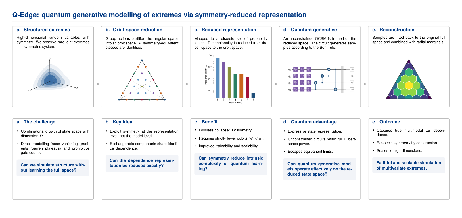
Q-Edge therefore connects multivariate extreme-value theory, symmetry-aware representation, and quantum generative modelling through a common computational principle: when dependence possesses exploitable structure, the appropriate object to learn is not the original high-dimensional distribution, but its exact representation over symmetry classes.
1.2 Structure of the Paper
The remainder of the paper is organized as follows. Section 2 introduces the Q-Edge framework and presents the symmetry-preserving orbit-space representation for multivariate extreme dependence. Section 3 develops the quantum generative learning architecture and discusses its implementation. Section 4 presents empirical results across a range of dependence structures, including nonlinear, heterogeneous, multimodal, geometrically constrained and high-dimensional settings. Section 5 concludes with implications for quantum digital twins, symmetry-aware learning and future research directions.
2 A Representation Principle for Structured Extreme Dependence
This section develops the theoretical foundation of Q-Edge. We show that exchangeability induces an exact orbit-space representation of multivariate extreme dependence, allowing the original dependence distribution to be represented losslessly on a substantially smaller state space. This symmetry-preserving representation changes the intrinsic complexity of the learning problem while preserving the dependence structure exactly. The resulting representation principle provides the basis for the quantum learning framework developed in the following section.
2.1 The Representation Bottleneck
The representation of multivariate extremes begins with the classical polar decomposition of multivariate extreme value theory. For a -dimensional random non-zero vector , an extreme event can be decomposed into its overall magnitude and its dependence structure through
The radial variable describes the severity of the extreme event, whereas the angular variable characterizes how the extremal magnitude is distributed across the variables. Since, under the regularly varying assumption, the radial component can be modelled independently using standard univariate extreme-value techniques, our interest lies entirely in the angular component, which completely specifies the dependence structure of multivariate extremes. The angular variable takes values on the probability simplex
whose dimension is . Each point on the simplex represents one possible allocation of the extremal magnitude among the variables, thereby providing a geometric representation of multivariate extreme dependence.
To enable statistical learning and quantum computation, the continuous simplex are usually approximated by a finite state space. Following the standard lattice discretization, we partition using the natural lattice
| (1) |
where denotes the discretization resolution. Normalizing each lattice point by establishes a one-to-one correspondence between and the rational lattice points on . Consequently, every lattice point represents one Euclidean Voronoi cell of a partition of the simplex, and a probability distribution over cells provides a finite-dimensional approximation of the underlying angular measure. The consistency of this discretization is established in Appendix D.
The complexity of this representation is determined by the cardinality of the natural lattice,
| (2) |
which grows combinatorially with both the dimension and the discretization resolution . Even moderate dimensions produce an extremely large configuration space, making direct statistical learning increasingly difficult. Consequently, improving the fidelity of the approximation rapidly enlarges the number of admissible dependence configurations that must be represented. This growth occurs before any learning or optimization is performed, indicating that the principal challenge is fundamentally one of representation rather than computation.
2.2 The Combinatorial Barrier
The natural lattice provides a finite representation of multivariate extreme dependence. The remaining question is whether this representation can be learned efficiently. As we show below, the answer is generally negative. The combinatorial growth of the discretized dependence space propagates directly to the quantum representation, resulting in exponential state-preparation costs and severe optimization difficulties. These computational bottlenecks all stem from a common source: the assumption that every dependence configuration must be represented as an independent quantum state.
To enable quantum learning, the discretized dependence space is embedded into the computational basis of a quantum register. An -qubit system possesses exactly computational basis states, and therefore the smallest compatible register satisfies
| (3) |
Since the lattice cardinality is generally not a power of two, we augment the natural lattice with additional representative centroids , obtaining an augmented configuration space.
| (4) |
The augmentation establishes a one-to-one correspondence between lattice configurations and computational basis states while preserving the geometric structure of the discretized simplex.
This embedding exposes the computational consequences of the representation. A generic probability distribution over occupies a -dimensional Hilbert space. Preparing an arbitrary quantum state in such a space requires elementary quantum gates (Grover, 2000; Plesch and Brukner, 2011; Sanders et al., 2019), reflecting the exponential number of independent amplitudes that must be specified. Consequently, state preparation alone rapidly becomes the dominant computational cost as the representation grows.
The challenge extends beyond state preparation to quantum optimization. Highly expressive parameterized quantum circuits approach Haar-random unitaries, for which the variance of the training gradient decreases exponentially with the number of qubits, giving rise to the barren plateau phenomenon (McClean et al., 2018; Cerezo et al., 2021). As the representation size increases, optimization becomes progressively more difficult, while finite coherence times and gate noise further restrict the depth of trainable quantum circuits on noisy intermediate-scale quantum (NISQ) devices.
Importantly, these computational bottlenecks share a common origin. They do not arise because quantum circuits are inherently inefficient, but because every lattice configuration is represented as an independent quantum state. In structured multivariate extremes, however, many configurations encode identical dependence patterns under permutations of statistically equivalent variables. Treating all such configurations separately introduces substantial representational redundancy, which is then inherited by the quantum model.
The implication is fundamental. Scalability cannot be achieved merely by designing more expressive quantum circuits, because the computational complexity is inherited from the representation itself rather than the learning architecture. This naturally raises the following question: are all dependence configurations genuinely distinct? As we show in the next subsection, for multivariate data exhibiting exchangeability, statistically equivalent dependence configurations can be identified and represented by a much smaller orbit space without sacrificing any statistical information.
2.3 Exchangeability and the Orbit-Space Representation
For many multivariate, treating every discretized dependence configuration as distinct is unnecessary. Financial assets within the same sector (Poon et al., 2004; Engelke and Hitz, 2020), geographically or physically similar sites in environmental and hydrological studies (Tawn, 1990; Coles and Tawn, 1991), and interchangeable components in compositional data arising in geology, biology and the geosciences (Aitchison, 1982) may play statistically equivalent roles. In such settings, permuting the variable labels changes the representation but not the underlying dependence structure. This symmetry is captured by exchangeability.
A simple example illustrates the resulting redundancy. At resolution in dimension , the six configurations
differ only by permutations of their coordinates and therefore describe the same allocation pattern under the action of the symmetric group . Treating them as six independent learning targets enlarges the representation without adding statistical information. The same permutation symmetry arises in standard dependence models, including the symmetric Dirichlet family, the symmetric logistic model for multivariate extremes (Gumbel, 1960; Tawn, 1990), and symmetric forms of the logistic-normal distribution (Aitchison and Shen, 1980; Aitchison, 1982).
To formalize this idea, let denote the symmetric group acting on the coordinates by permutation. A distribution on the action closed augmented configuration space is exchangeable when its probability assignment is unchanged by this action.
Definition 1 (-symmetric distribution).
A probability distribution on is -symmetric, or equivalently -exchangeable, if
| (5) |
The set of all such distributions is denoted .
Exchangeability allows configurations related by permutations to be grouped together. The orbit of is
| (6) |
The distinct orbits partition into equivalence classes, and each orbit represents one dependence pattern together with all of its possible coordinate labellings.
The resulting collection of symmetry classes is the orbit space
We denote its cardinality by Explicit orbit counts and the extension to subgroups , including block-symmetric groups associated with partial exchangeability, are provided in the Appendix (Theorem 21, Theorem 15, and Proposition 12).
Because an exchangeable distribution is constant within each orbit, it is completely determined by one probability value per orbit rather than one value per configuration. Symmetry therefore changes the intrinsic dimension of the statistical model.
Proposition 1 (Dimension under exchangeability).
The space of -symmetric probability distributions on has dimension
| (7) |
A proof is given in the Appendix (Proposition 7). Proposition 1 shows that the relevant representation complexity is governed by the number of distinct symmetry classes, rather than by the total number of lattice configurations. When the orbits are large, this produces a substantial reduction in dimension before any learning algorithm is applied.
2.4 Lossless Orbit-Space Representation
The orbit construction reduces the number of configurations that must be represented. The remaining question is whether this reduction discards statistical information. For exchangeable distributions, it does not: the orbit space provides an exact reformulation of the original learning problem.
Let denote the distinct orbits in , and let be the size of the th orbit. The probability simplex over the orbit space is
| (8) |
Here, denotes the total probability mass assigned to the entire orbit . To recover a distribution on the original configuration space, this mass is distributed uniformly among the configurations belonging to the orbit. Let denote the index of the orbit containing . We define the orbit map
| (9) |
The map converts an orbit-level probability distribution into an exchangeable distribution on . The following result shows that this representation is lossless.
Theorem 1 (Lossless orbit-space representation).
The orbit map
is a bijection. Thus, every -symmetric distribution on has a unique representation in the orbit simplex.
Moreover, preserves total variation distance:
| (10) |
for all . It also preserves every -divergence for which the divergence is well defined, including the symmetric Kullback–Leibler divergence used during training.
The proof, together with the corresponding weighted-inner-product isometry, is given in the Appendix (Theorem 20).
Theorem 1 establishes that orbit-space representation is not an approximation or a lossy compression. Every exchangeable distribution corresponds to exactly one orbit-space distribution, and the statistical discrepancies used for learning are preserved. Optimizing total variation or KL divergence in the orbit space is therefore equivalent to optimizing the same objective in the full configuration space.
The reduction is purely representational. A general distribution on requires
degrees of freedom, whereas an exchangeable distribution requires only
The corresponding representation ratio is
| (11) |
When many configurations belong to the same symmetry orbit, , yielding a substantial reduction in both classical and quantum representation complexity.
This result identifies exchangeability as a representation principle, rather than merely an inductive bias imposed on a learning architecture. Q-Edge removes symmetry-induced redundancy before learning begins and operates directly on the smaller orbit simplex. The next section develops the quantum realization of this lossless representation.
3 Q-Edge: A Symmetry-Aware Quantum Representation
The previous section established the representation principle of Q-Edge. Exchangeability identifies statistically equivalent dependence configurations, the orbit-space representation removes this redundancy without loss of information, and the resulting orbit simplex provides a compact representation of multivariate extreme dependence. We now show how this representation is realized on a quantum computer.
Q-Edge consists of four stages (Fig. 2). First, extreme observations are represented through the angular component of multivariate extreme value theory. Second, the angular simplex is discretized into a quantum representation compatible with finite qubit registers. Third, we show that representing arbitrary dependence distributions is fundamentally impossible for hardware-efficient quantum circuits because of an intrinsic representation barrier. Finally, Q-Edge overcomes this barrier by learning directly in the orbit space, where exchangeability reduces the statistical complexity before any quantum resources are used.
3.1 Representing Extremes
Following the polar decomposition of multivariate extreme value theory, Q-Edge models only the angular component describing extremal dependence. The radial magnitude is asymptotically independent of and is therefore modelled separately. The complete extreme sample is recovered as
The angular distribution is represented by a quantum circuit Born machine (QCBM),
where the circuit parameters depend smoothly on the radial magnitude through
This parameterization ensures that the learned angular distribution approaches a radius-independent limit as , consistent with extreme value theory. As a design choice we therefore restrict to a hardware-efficient ansatz of gate complexity .
Theorem 2 (Lipschitz continuity).
Let be the Born distribution of our parameterized circuit. The Born distribution varies continuously with the radial magnitude. Specifically,
where depends only on the parameterization coefficients. A refined bound and proof are given in the Appendix.
The theorem provides a theoretical guarantee that nearby extreme events produce nearby angular distributions, enabling stable conditioning on event.
3.2 Representing the Angular Simplex
To represent angular dependence on a quantum computer, the continuous simplex is discretized into a finite collection of Voronoi cells, each corresponding to one computational basis state.
A natural lattice of resolution contains cells, which in general is not a power of two, satisfying Consequently, a direct encoding either discards surplus basis states or introduces penalty terms, both of which reduce representation efficiency.
Q-Edge resolves this mismatch by augmenting the lattice with geometrically canonical centroid points. For a base lattice point and a type- elementary simplex, the corresponding centroid is
| (12) |
where the derivation is given in Appendix E. Selecting an appropriate subset of these centroids produces an augmented grid satisfying thereby establishing a bijection Every computational basis state is therefore assigned to exactly one simplex cell, eliminating both unused basis states and artificial penalty terms. The resulting discretization is statistically consistent.
Theorem 3 ( convergence of the discretization).
Let with density , and let denote the piecewise-constant projection induced by . Then
The proof is given in Appendix D. Consequently, the total approximation error separates naturally into
| (13) |
By Theorem 3, the discretization error vanishes asymptotically. The remaining limitation therefore lies not in the representation of the simplex, but in the expressive power of the quantum model.
3.3 The Fundamental Representation Barrier
The augmented discretization developed in the previous subsection eliminates approximation error in the representation of the angular simplex. A natural question therefore arises: can a hardware-efficient quantum circuit accurately represent an arbitrary dependence distribution?
The following theorem shows that the answer is fundamentally negative. The limitation is not a consequence of a particular circuit design or optimization algorithm, but of the intrinsic dimension of the probability simplex itself.
Theorem 4 (Fundamental representation barrier).
Let denote the family of probability distributions reachable by a parameterized quantum circuit with trainable parameters acting on qubits, and let . If , then there exists a probability distribution satisfying
where
The proof is given in Appendix C.
Theorem 4 establishes a fundamental representation barrier for quantum generative models. For the hardware-efficient scaling , as . Any circuit with only polynomially many trainable parameters is necessarily unable to represent arbitrary probability distributions on the full -state simplex. This limitation is independent of the choice of ansatz, optimizer or training algorithm; it arises solely from the intrinsic dimension of the statistical model.
Consequently, improving the quantum circuit alone cannot overcome this barrier. The representation itself must change. The next subsection shows that exchangeability provides exactly such a change: by replacing the original configuration space with its orbit-space representation, the effective dimension is reduced from to the orbit count, making accurate learning compatible with hardware-efficient quantum circuits.
3.4 Escaping the Barrier through Symmetry
Q-Edge overcomes the representation barrier by exploiting the exchangeability developed in Section 2. Rather than learning over the original configuration space, the quantum circuit operates directly on the orbit simplex.
The orbit-space representation replaces the original configuration states by
orbit representatives, requiring only qubits. Each computational basis state now represents an entire symmetry class rather than a single lattice configuration.
This leads to a fundamentally different learning problem. Instead of approximating distributions on the full simplex, the circuit learns only the orbit-space distribution. By Theorem 1, this representation is lossless, so optimization in orbit space is mathematically equivalent to learning the original exchangeable distribution.
The resulting architecture differs fundamentally from existing equivariant quantum circuits. Rather than constraining the circuit to preserve symmetry, Q-Edge removes symmetry-induced redundancy before learning begins. The quantum circuit therefore remains completely unconstrained while producing an exactly exchangeable distribution through the orbit-space representation.
Theorem 5 (Orbit-space dominance).
Every distribution reachable by an equivariant quantum circuit is also reachable by the orbit-space construction, while requiring no more parameters and, whenever , strictly fewer qubits.
The degree of compression depends only on the underlying symmetry. Fully symmetric dependence models achieve more than forty-fold reductions in representation size, whereas asymmetric models recover the original representation (Table 1).
The key innovation of Q-Edge is therefore not a more expressive quantum circuit but a different representation on which the circuit operates. By exploiting exchangeability before learning begins, Q-Edge transforms an intractable representation problem into one compatible with near-term quantum hardware while preserving the statistical structure of multivariate extremes exactly.
3.5 Symmetry as an escape: the orbit-space construction
The representation barrier established in Theorem 4 applies to arbitrary probability distributions on the full simplex. Many dependence distributions arising in practice, however, exhibit exchangeability or partial exchangeability. The orbit-space representation introduced in Section 2 changes the statistical model itself by replacing the full simplex with the symmetric simplex , whose dimension is
| (14) |
where denotes the number of symmetry orbits. Since for highly symmetric problems, the intrinsic dimension of the target distribution is dramatically reduced.
The consequence is immediate. The representation barrier of Theorem 4 applies to the intrinsic dimension of the target simplex. Replacing the original simplex by changes the necessary parameter requirement from to Thus the escape from the representation barrier comes not from a more expressive quantum circuit, but from representing a lower-dimensional statistical model.
The amount of compression depends only on the orbit count. For the Dirichlet family, the orbit count can be computed explicitly using Burnside’s lemma (Appendix E Theorem 22). Table 1 illustrates the continuous transition from fully asymmetric to fully symmetric targets. For example, when and with block symmetry , the original discretization contains approximately cells (about 21 qubits), whereas the orbit-space representation contains only states.
| Target | Symmetry | Compression | ||
|---|---|---|---|---|
To realize this reduced representation on a quantum computer, we encode the orbit indices directly rather than the original simplex cells. Choosing , we introduce a bijection and represent the Born distribution over orbit indices, The probability assigned to each orbit is then distributed uniformly over its members,
Unlike equivariant quantum circuits, this construction imposes no symmetry constraint on the circuit itself. Symmetry is enforced entirely through the statistical representation.
4 Results
We evaluate Q-Edge through three questions that correspond directly to the theoretical developments. First, does the orbit-space representation itself overcome the representation barrier? Second, does Q-Edge outperform existing classical generative models for structured extreme dependence? Finally, does the representation remain effective in high-dimensional settings where direct quantum representations become impractical? To answer these questions, we evaluate Q-Edge on five synthetic -symmetric dependence distributions in three dimensions and on a challenging 30-dimensional -symmetric Dirichlet distribution. Throughout, Q-Edge is compared against a direct-cell quantum circuit Born machine using the same circuit architecture and training procedure and, where appropriate, a parameter-matched conditional variational autoencoder (VAE). Performance is assessed using three complementary metrics: root mean squared error (RMSE), symmetric Kullback–Leibler (KL) divergence, and total variation distance (TVD). RMSE measures the pointwise accuracy of the reconstructed density, symmetric KL divergence quantifies distributional fidelity, and TVD measures the global probability mass discrepancy. Together, these complementary metrics show that the improvement is systematic rather than metric-specific. Implementation details, objective function, model architectures, optimization procedures, hyperparameter settings, and hardware implementation are deferred to Appendix A.
4.1 Does Orbit-Space Representation Overcome the Representation Barrier?
The central claim of Q-Edge is that the primary limitation is not the quantum circuit itself, but the statistical representation on which it operates. To isolate this effect, we compare two quantum circuit Born machines that share exactly the same circuit architecture, optimization procedure and target distributions. The only difference is the representation: Direct - one circuit learns directly on the discretized simplex, whereas Q-Edge learns on the symmetry-reduced orbit simplex.
We consider five radius-conditioned, -symmetric dependence distributions defined on the 2-simplex (Appendix A.1), covering a broad spectrum of extremal dependence geometries, including unimodal, multimodal, vertex-concentrated, barycentre-concentrated and curved-support distributions. We focus on three-dimensional dependence structures because they provide the simplest non-trivial setting in which exchangeability, multimodality, and complex extremal dependence can all be systematically evaluated while remaining fully visualizable. Both models employ the same -CNOT ansatz and identical radius-conditioned training. At resolution , the augmented simplex contains cells, which the symmetry reduces to orbit classes. Consequently, the orbit-space model operates on only four qubits, whereas the direct-cell representation requires six.
Q-Edge consistently improves reconstruction accuracy across all five target distributions, providing lower reconstruction error than the direct-cell QCBM across all three evaluation metrics (Table 2). Even for the Dirichlet distribution, where both models achieve highly accurate reconstructions, Q-Edge reduces RMSE by 31%, symmetric KL divergence by 50%, and TVD by 35%. The improvement becomes even more pronounced for geometrically complex dependence structures. For the logistic-normal and ring distributions, symmetric KL divergence is reduced by 73% and 75%, respectively, accompanied by substantial reductions in both RMSE and TVD. Averaged across all five targets, Q-Edge reduces RMSE by 30%, symmetric KL divergence by 53%, and TVD by 36%. Q-Edge more faithfully preserves multimodal and curved-support dependence structures while the direct-cell model exhibits visible symmetry-breaking artefacts.
These improvements cannot be attributed to increased model capacity. Indeed, the direct-cell QCBM employs a larger Hilbert space, two additional qubits and a correspondingly larger parameter space. The only difference between the two models is the statistical representation on which optimization is performed. Q-Edge operates directly in the exchangeable probability simplex, where every feasible point satisfies the required permutation symmetry. In contrast, the direct-cell model searches the full probability simplex, whose vast majority of candidate distributions violate the symmetry of the target. Consequently, a substantial fraction of the optimization effort is spent exploring regions that are statistically irrelevant.
Q-Edge / Direct-QCBM (relative improvement) RMSE () Sym. KL () TVD () Dirichlet () () () Logistic spectral () () () Logistic-normal () () () Three-mode () () () Ring () () ()
These results provide direct empirical evidence for the representation principle. The observed performance gain does not arise from a more expressive quantum circuit, but from performing optimization in the correct statistical space. Orbit-space compression simultaneously reduces the computational dimension, enforces exchangeability exactly, and improves reconstruction accuracy, thereby overcoming the representation barrier predicted by Theorem 4.
4.2 Can Orbit-Space Quantum Learning Outperform Classical Generative Models?
Having established that orbit-space representation overcomes the representation barrier independently of circuit architecture, we next compare Q-Edge with a classical deep generative model. The objective is not to compare quantum and classical hardware, but to determine whether the combination of symmetry-aware representation and quantum generative learning provides a statistical advantage over a parameter-matched classical baseline.
We evaluate both models on the same five radius-conditioned, -symmetric dependence distributions defined on the 2-simplex. At resolution , the augmented partition contains cells, which collapse to orbit states under the symmetry, allowing the entire problem to be represented on six qubits. Q-Edge learns directly on the orbit simplex, whereas the baseline is a conditional variational autoencoder (VAE) with a Dirichlet decoder and a comparable parameter budget. Both models are trained using the same adaptive partition and evaluated on eleven held-out radii spanning .
Q-Edge / VAE (relative improvement) RMSE () Sym. KL () TVD () Dirichlet () () () Logistic spectral () () () Logistic-normal () () () Three-mode () () () Ring () () ()
The Dirichlet distribution represents a special case because it belongs to the native decoder family of the VAE. Consequently, the classical model achieves better reconstruction. Nevertheless, both methods already attain near-perfect accuracy, with all three error metrics remaining close to zero, indicating that the practical difference between the two approaches is negligible. Outside this favourable setting, Q-Edge consistently outperforms the classical baseline. The largest gains are observed for the logistic-normal, ring and three-mode distributions, whose complex geometric structures deviate substantially from the Dirichlet family. For these challenging targets, Q-Edge reduces distributional errors by up to and improves pointwise reconstruction accuracy by up to .
These improvements arise from fundamentally different inductive biases. The VAE inherits a strong preference for Dirichlet-like distributions through its decoder, explaining its excellent performance on the Dirichlet benchmark but limiting its ability to represent multimodal and curved-support dependence. In contrast, Q-Edge imposes no parametric assumption on the target distribution. Instead, it learns directly in the exchangeable orbit space, allowing the quantum circuit to represent the full class of symmetric probability distributions.
The reconstructed densities (Fig. 3) reveal qualitative differences that are not fully captured by scalar error metrics. While both methods accurately recover the simple Dirichlet distribution, the VAE progressively smooths multimodal and curved-support dependence structures towards simpler unimodal distributions. In contrast, Q-Edge faithfully reconstructs multiple peaks, ring-shaped support and sharp geometric features, reflecting its ability to learn directly within the space of exchangeable probability distributions without imposing a restrictive parametric decoder.
Figure 4 explains why these qualitative differences arise. As the radius increases, the three-mode distribution develops increasingly separated modes, while the ring distribution concentrates probability mass along a curved manifold. These geometric changes have little effect on Q-Edge, whose reconstruction errors remain consistently low across the full range of radii. By contrast, the VAE errors increase substantially once the target departs from the Dirichlet family, indicating that its inductive bias becomes increasingly restrictive as the dependence geometry grows more complex.


4.3 Does Orbit-Space Compression Enable Scalable Quantum Learning?
Having demonstrated the statistical advantages of orbit-space learning in low-dimensional settings, we finally investigate whether these advantages persist at a practically relevant scale. The theoretical analysis predicts that orbit-space compression transforms an otherwise combinatorial representation into a polynomially growing one. We test this prediction on a 30-dimensional dependence distribution whose full partition is far beyond the capacity of a direct quantum encoding.
The target is a radius-conditioned Dirichlet distribution on with three concentration parameters assigned to three blocks of ten exchangeable variables, giving symmetry group . At partition resolution , the augmented grid contains cells, requiring approximately 21 qubits under a direct encoding. Exploiting permutation symmetry reduces the representation to
orbit states, corresponding to a compression of the state space. Consequently, the entire learning problem can be solved using only eight qubits, exactly as predicted by the orbit-space construction.
The orbit-space QCBM is trained using symmetric KL divergence with 3 456 trainable parameters (35 circuit layers and radial order ), comfortably satisfying the necessary condition . As a classical baseline, we employ a parameter-matched conditional VAE whose Dirichlet decoder is explicitly constrained to satisfy the same symmetry. Both models therefore learn within the identical exchangeable probability space, allowing the comparison to isolate differences in learning capability rather than differences in expressive capacity.
Unlike the three-dimensional examples, a 30-dimensional dependence distribution cannot be visualized directly on the simplex. We therefore compare the reconstructed per-point densities over the 256 orbit states. Each histogram reports the probability assigned to every symmetry-equivalent orbit, providing a direct visualization of how accurately each model reconstructs the high-dimensional probability geometry while preserving exchangeability.
The comparison is intentionally stringent because the target distribution belongs to the native decoder family of the VAE (Table 4). Consequently, the VAE achieves a lower symmetric KL divergence, consistent with the three-dimensional Dirichlet benchmark. This advantage is expected, as the decoder is parameterized by the correct distribution family.
In contrast, the orbit-space QCBM makes no assumption about the functional form of the target distribution. Nevertheless, it reduces the per-point RMSE by approximately and the total variation distance by relative to the VAE, indicating a more accurate reconstruction of the local probability geometry while remaining competitive in overall distributional fidelity.
Both models accurately recover the target distribution across all eleven held-out radii, while the orbit-space QCBM more faithfully captures fine-scale probability variations among neighbouring orbit states. These qualitative differences are consistent with the lower RMSE and TVD achieved by Q-Edge, whereas the VAE retains a slight advantage in symmetric KL because the target lies exactly within its assumed Dirichlet decoder family.
More importantly, these results demonstrate that orbit-space compression preserves statistical accuracy while fundamentally changing the computational scale of the learning problem. A direct encoding would require representing more than million partition cells (approximately qubits), whereas the symmetry-reduced representation requires only orbit states (eight qubits), a reduction in state-space size. Orbit-space compression therefore transforms an otherwise intractable high-dimensional quantum learning problem into one that is compatible with near-term quantum hardware without sacrificing reconstruction quality.
| RMSE | Sym. KL | TVD | |
|---|---|---|---|
| Dirichlet | () | () | () |
| Logistic normal | () | () | () |
| Three-mode mixture | () | () | () |
5 Discussion
The central contribution of this work is conceptual rather than algorithmic. We show that the principal obstacle to quantum generative modelling of multivariate extremes is not limited circuit expressivity, but an inappropriate statistical representation. Classical and quantum models alike are typically trained in the full probability simplex, whereas the target distributions occupy a much smaller symmetry-constrained manifold. By learning directly in the orbit space, Q-Edge aligns the model representation with the statistical structure of exchangeable extremes, transforming an exponentially large learning problem into an equivalent low-dimensional one.
This perspective establishes a different route towards scalable quantum machine learning. Rather than overcoming expressivity limitations by increasing circuit size or depth, orbit-space compression exploits representation-theoretic structure before optimization begins. The resulting reduction preserves the target distribution exactly while substantially decreasing the effective dimension of the learning problem. Our theoretical analysis identifies the conditions under which such compression is lossless, and the numerical experiments demonstrate that it leads to improved statistical accuracy despite requiring fewer qubits and fewer effective degrees of freedom.
The present work also clarifies the role of quantum computing in learning extreme dependence. The quantum advantage does not arise from representing arbitrary high-dimensional distributions, but from efficiently modelling structured probability spaces whose symmetry makes them intrinsically compressible. Although demonstrated here for exchangeable multivariate extremes, the underlying principle extends naturally to other generative modelling problems possessing group symmetries.
Several limitations remain. The experiments are performed using exact statevector simulation, and the robustness of the approach under hardware noise and finite sampling remains to be established. In addition, the largest experiments remain within the classically simulable regime, demonstrating the correctness and scalability of the orbit-space construction rather than a computational quantum advantage. Finally, the current framework assumes that the underlying symmetry is known exactly; extending orbit-space learning to approximately symmetric or data-driven group structures is an important direction for future research.
More broadly, Q-Edge suggests that exploiting statistical symmetry may be as important as improving quantum hardware for scalable quantum machine learning. Orbit-space compression provides a general mechanism for matching quantum representations to structured probability spaces, opening opportunities well beyond extreme-value modelling, including scientific machine learning, probabilistic digital twins, and high-dimensional stochastic simulation.
References
- Logistic-normal distributions: some properties and uses. Biometrika 67 (2), pp. 261–272. External Links: Document Cited by: §2.3.
- The statistical analysis of compositional data. Journal of the Royal Statistical Society: Series B (Methodological) 44 (2), pp. 139–160. External Links: Document Cited by: §2.3, §2.3.
- Cost function dependent barren plateaus in shallow parametrized quantum circuits. Nature Communications 12 (1), pp. 1791. External Links: Document Cited by: §2.2.
- Modelling extreme multivariate events. Journal of the Royal Statistical Society: Series B (Methodological) 53 (2), pp. 377–392. External Links: Document Cited by: §2.3.
- Generative modelling of multivariate geometric extremes using normalising flows. External Links: 2505.02957, Document, Link Cited by: §1.1.1, §1.1.2.
- Introduction to quantum control and dynamics. Chapman and hall/CRC. Cited by: Remark 18.
- Graphical models for extremes. Journal of the Royal Statistical Society: Series B (Statistical Methodology) 82 (4), pp. 871–932. External Links: Document Cited by: §1.1.2, §2.3.
- Cryptographic distinguishability measures for quantum-mechanical states. IEEE transactions on information theory 45 (4), pp. 1216–1227. Cited by: Definition 4.
- Generative adversarial networks. Communications of the ACM 63 (11), pp. 139–144. Cited by: §1.1.1.
- A kernel two-sample test. The journal of machine learning research 13 (1), pp. 723–773. Cited by: §A.1.
- Synthesis of quantum superpositions by quantum computation. Physical Review Letters 85 (6), pp. 1334–1337. Cited by: §2.2.
- Bivariate exponential distributions. Journal of the American Statistical Association 55 (292), pp. 698–707. External Links: Document Cited by: §2.3.
- GPDFlow: generative multivariate threshold exceedance modeling via normalizing flows. External Links: 2503.11822, Document, Link Cited by: §1.1.1.
- Auto-encoding variational bayes. arXiv preprint arXiv:1312.6114. Cited by: §1.1.1.
- A vae approach to sample multivariate extremes. Journal of Statistical Computation and Simulation, pp. 1–37. Cited by: §1.1.1, §1.1.2.
- Diagnosing barren plateaus with tools from quantum optimal control. Quantum 6, pp. 824. External Links: Document Cited by: §1.1.3, Remark 18.
- Group-invariant quantum machine learning. PRX quantum 3 (3), pp. 030341. Cited by: §E.4, §1.1.3.
- Simulation of multivariate extremes: a Wasserstein–Aitchison GAN approach. Extremes. External Links: Document, Link Cited by: §1.1.1, §1.1.2.
- Differentiable learning of quantum circuit born machines. Physical Review A 98 (6), pp. 062324. Cited by: §A.1, §1.1.3, §1.1.4.
- Mitigation of readout noise in near-term quantum devices by classical post-processing based on detector tomography. Quantum 4, pp. 257. Cited by: §A.2.
- Barren plateaus in quantum neural network training landscapes. Nature Communications 9 (1), pp. 4812. External Links: Document Cited by: §2.2.
- COMET flows: towards generative modeling of multivariate extremes and tail dependence. In Proceedings of the Thirty-First International Joint Conference on Artificial Intelligence (IJCAI), pp. 3328–3334. External Links: Document Cited by: §1.1.1.
- Exploiting symmetry in variational quantum machine learning. PRX quantum 4 (1), pp. 010328. Cited by: §1.1.3.
- Quantum circuit learning. Physical Review A 98 (3), pp. 032309. Cited by: §1.1.3.
- Deep learning of multivariate extremes via a geometric representation. External Links: 2406.19936, Document, Link Cited by: §1.1.1, §1.1.2.
- Scalable mitigation of measurement errors on quantum computers. PRX Quantum 2 (4), pp. 040326. Cited by: §A.2.
- Theory for equivariant quantum neural networks. PRX quantum 5 (2), pp. 020328. Cited by: §1.1.3.
- Quantum computation and quantum information. Cambridge university press. Cited by: §B.4, §E.4.2.
- Quantum-state preparation with universal gate decompositions. Physical Review A 83 (3), pp. 032318. Cited by: §2.2.
- Extreme value dependence in financial markets: diagnostics, models, and financial implications. The Review of Financial Studies 17 (2), pp. 581–610. External Links: Document Cited by: §2.3.
- A Lie algebraic theory of barren plateaus for deep parameterized quantum circuits. Nature Communications 15 (1), pp. 7172. External Links: Document Cited by: §1.1.3.
- Heavy-tail phenomena: probabilistic and statistical modeling. Springer. Cited by: §1.1.2.
- Variational inference with normalizing flows. In International conference on machine learning, pp. 1530–1538. Cited by: §1.1.1.
- Multivariate generalized pareto distributions. Bernoulli 12 (5), pp. 917–930. Cited by: §1.1.2.
- Black-box quantum state preparation without arithmetic. Physical Review Letters 122 (2), pp. 020502. Cited by: §2.2.
- Theoretical guarantees for permutation-equivariant quantum neural networks. npj Quantum Information 10 (1), pp. 12. Cited by: §E.4, §1.1.3.
- Modelling multivariate extreme value distributions. Biometrika 77 (2), pp. 245–253. External Links: Document Cited by: §2.3, §2.3.
- Mitigating depolarizing noise on quantum computers with noise-estimation circuits. Physical review letters 127 (27), pp. 270502. Cited by: §A.2.
- Generative machine learning for multivariate angular simulation. Extremes. Note: Preprint arXiv:2504.21505 titled “A comparison of generative deep learning methods for multivariate angular simulation” External Links: Document, Link Cited by: §1.1.1, §1.1.2.
- Diffusion models: a comprehensive survey of methods and applications. ACM computing surveys 56 (4), pp. 1–39. Cited by: §1.1.1.
- Quantum generative adversarial networks for learning and loading random distributions. npj Quantum Information 5 (1), pp. 103. Cited by: §1.1.3.
Appendix
Appendix A Implementation
A.1 Experiment Setup
Training and the orbit-space encoding.
The ansatz and its parameter count are specified under the rational radial parameterisation of Eq. (17). The orbit-space route places no symmetry constraint on the entangler, and the simulations use the circular-CNOT layer; for the hardware runs we use the equivalent cyclic-CZ layer, whose gates pairwise commute and therefore compile to half the depth on devices whose native two-qubit gate is CZ. The equivariant baseline, by contrast, requires an entangler invariant under the induced qubit permutations, which is what motivates the full-CZ layer there (Appendix, Definition 22). The circuit is trained by minimizing the symmetric KL divergence (Jeffreys divergence) between the Born distribution and the target cell masses,
| (15) |
Training minimises the summation of over the representative radii of the adaptive bins of Eq. (62) (),
| (16) |
both computed in closed form from the statevector. The choice of divergence is principled: for the bounded Gaussian-mixture kernels standard in Born-machine training (Gretton et al., 2012; Liu and Wang, 2018), with , one has by the reproducing property and Pinsker’s inequality, so driving the symmetric KL to zero forces the MMD (and the total variation) to zero. The converse fails: a bounded kernel is insensitive to likelihood ratios, so the MMD can be arbitrarily small while the KL divergence remains large—or infinite, when the model assigns vanishing mass where the target does not. Exact statevector simulation makes the KL computable without sampling, removing the estimation advantage that usually motivates the MMD. For the orbit-space model, is chosen to be a power of two, qubits are used, and is fixed by barycentre anchoring, sorting and Gray coding (Section 3.5). The Dirichlet specialisation of Burnside’s lemma reads , where is the number of partitions of into at most parts (Appendix, Theorem 22).
Target distributions (2-simplex).
All five radius-conditioned targets are -invariant on . The Dirichlet target is symmetric with , which decays through the uniform law ( at ) toward vertex-favouring concentration. The logistic spectral measure has density with , moving from vertex-concentrated near-independence at to barycentre-concentrated near-complete dependence as . The logistic-normal is an Aitchison density with exchangeable log-ratio covariance and . The three-mode mixture is with , ranging from near-uniform at to three sharp peaks at the edge midpoints as . The circle is an annulus of width centred at with radius , projected to barycentric coordinates.
Implementation and metrics.
The orbit-space QCBM ( qubits, , ) is implemented in PennyLane (default.qubit, backpropagation). Training uses Adam with a cosine-annealed learning rate and gradient clipping, minimising the exact symmetric-KL objective; targets are cached on the adaptive radial boundaries of Eq. (62) (, ). For the experiment (, , ) the same protocol is used. The classical baseline on the 2-simplex is a conditional VAE with a Dirichlet decoder (latent dimension , parameter count matched to the quantum model), trained by standard ELBO on samples drawn at the same radial boundaries and evaluated by Monte-Carlo marginalisation of its decoder at the grid points, normalised to the point-density semantics used for the QCBM and the analytic target. In thirty dimensions the baseline is itself constrained to be invariant, at parameters against for the quantum model; the baseline is therefore favoured on both counts, searching the and doing so with more parameters. Its latent variable is active on every target (final between and nats over a three-dimensional latent), so the comparison is not confounded by posterior collapse. Reported metrics—RMSE, symmetric KL divergence, and total-variation distance.
A.2 Execution on quantum hardware
The orbit-space construction compresses the , angular grid from points to exchangeability orbits under the full symmetric group , so the Born machine requires qubits. To ensure the model possesses adequate capacity to learn arbitrary distributions, we conservatively set the quantum circuit depth to . We verify that this compression makes the model executable on present-day hardware by running the trained Dirichlet model on two IBM processors of different coupling topology: ibm_miami, a -qubit Nighthawk device with a square lattice, and ibm_pittsburgh, a -qubit Heron device with a heavy-hexagonal lattice. Training is performed classically; the devices are used only for inference, i.e. to sample at eleven held-out values of . Both runs execute the same logical circuit at the same angles: the angle matrix obtained from the classical optimization is stored and replayed on the second device, so the two executions differ only in how that circuit is compiled onto the hardware. The noiseless reference is recomputed from those same angles and is therefore identical for both, which is what makes the comparison controlled.
The two topologies compile this circuit differently, and that difference is the object of the comparison. The Nighthawk lattice is a square grid and so contains four-cycles; the cyclic entangler therefore maps onto physical couplings with no routing overhead, and the compiled circuit contains exactly two-qubit gates at depth . The heavy-hexagonal lattice contains no four-cycles, so the same ring requires inserted swap operations and compiles to two-qubit gates at depth —a overhead in gate count. This is a property of the coupling graph rather than of the construction, and we report it so that the gate counts can be attributed correctly, not as an advantage of the method.
| ibm_miami | ibm_pittsburgh | |
| (Nighthawk, square) | (Heron, heavy-hex) | |
| Qubits / orbits / grid points | / / (compression ) | |
| Layers / polynomial order | / | |
| Effective parameters | ||
| Angle matrix | identical (replayed from the first run) | |
| Two-qubit gates (logical / compiled) | / | / |
| Inserted swap | none | yes |
| ISA depth | ||
| Shots per | ||
| Mirror / readout calibration | / shots circuits | |
| Dynamical decoupling / twirling | XpXm / gates and measurement | |
Result.
Comparing a finitely sampled hardware distribution against an analytically evaluated simulator distribution is not like-for-like: at and outcomes, multinomial sampling alone contributes in total variation, comparable to the model error itself. We therefore quote all ratios against a shot-matched baseline obtained by drawing samples from the noiseless model distribution.
Table 6 gives the outcome. Two standard corrections are applied on each device, in sequence and in the reverse order of the channels they undo: readout first, then depolarizing. Neither uses the target, and both are calibrated from separate circuits. The readout step is confusion-matrix unfolding (Maciejewski et al., 2020; Nation et al., 2021); with only four qubits we measure the full matrix from sixteen basis-state preparations rather than the tensor-product approximation used at larger registers, and solve for the corrected distribution by constrained least squares, which returns a valid probability vector where direct inversion would not. The depolarizing step follows the noise-estimation-circuit method of Urbanek et al. (2021), with the mirror circuit as the estimator; because the mirror carries twice the entangling gates, the factor for a single execution is taken as the square root of the measured one, and it is estimated separately at each radius rather than once for the run. Gate and measurement twirling are enabled throughout, which is what makes a single-parameter depolarizing model a reasonable ansatz. After both, the learned angular measure is reproduced to within the shot-matched baseline in total variation on the square lattice and on the heavy-hexagonal one, with absolute total variation distances of and over the -point grid.
| RMSE | TVD | |||
| Noiseless simulator, exact | ||||
| Noiseless simulator, shot-matched | ||||
| ibm_miami — square lattice, two-qubit gates | ||||
| raw | ||||
| readout | ||||
| depolarizing | ||||
| ratio to shot-matched | ||||
| ibm_pittsburgh — heavy-hex lattice, two-qubit gates | ||||
| raw | ||||
| readout | ||||
| depolarizing | ||||
| ratio to shot-matched | ||||
Error budget and the effect of topology.
Because the target is -invariant it is constant within each orbit, and the decoder spreads orbit mass uniformly; grid-space and orbit-space total variation distances therefore coincide, allowing the three error sources to be separated. Referencing hardware output to the noiseless simulator rather than to the target isolates the device contribution, giving post-mitigation device residuals of and against a common model approximation error of and a common sampling floor of . Combining these in quadrature—an approximation, since total variation is not an norm, but one that reproduces the measured residual to within —the device accounts for and of the total error budget, sampling for and , and the model for on both: the fidelity reported above is limited by the processors, not by the ansatz or the shot budget.
The topological difference enters as predicted, but is partly offset. The mirror-circuit depolarizing factor falls from on the square lattice to on the heavy-hexagonal one, consistent with the larger gate count; solving for gives per-gate depolarizing rates of and , close enough that the difference in is attributable to gate count rather than gate quality. The final fidelities, however, differ by only in total variation, because the heavy-hexagonal device has markedly better readout: readout mitigation removes of the raw residual there against on the square lattice, offsetting much of the routing overhead.
A second difference is structural rather than aggregate. On the square lattice the post-mitigation residual varies by a factor of across and is strongly correlated with the angle-schedule variable (Pearson ), with the implied error strength spanning ; on the heavy-hexagonal device the same residual varies by only (correlation , span ). Since the gate count is identical for every and only the rotation angles differ, a stochastic channel of fixed strength cannot produce such a dependence: an angle-dependent, coherent component remains identifiable on the shallower circuit, whereas on the deeper one the larger stochastic error masks it. Removing that component would require learning the device’s Pauli–Lindblad generator, which we do not attempt here; the purpose of this section is to establish executability rather than to optimise hardware performance.
We note two limitations. The two executions are separated in time and therefore differ in calibration state as well as in topology, so drift cannot be excluded as a contributor to the differences reported above; and each configuration was run once, so the residual structure—in particular the correlation of —would benefit from replication.

Appendix B The Parameterized Quantum Circuit
B.1 Setup and Notation
Consider an -qubit parameterized quantum circuit (PQC) with entangling layers.
Definition 2 (Circuit architecture).
The circuit acts on qubits with entangling layers, defined by:
- 1.
Initial layer: Hadamard gates on all qubits, .
- 2.
Parameterized blocks (): For each qubit , apply the decomposition:
where and .
- 3.
Entangling layers (): After each parameterized block (except the last), apply a circular CNOT ladder :
The total number of variational parameters is .
In the layer-level representation, the full unitary reads:
| (17) |
Since gates acting on different qubits commute, each tensor product can be expanded into a sequential product in any order. Assigning a global index to the parameterized rotation gates—ordered so that is applied first (immediately after ) and is applied last (closest to the measurement end)—and absorbing all fixed gates (CNOT layers and identity operators between commuting single-qubit blocks) into fixed (parameter-independent) unitaries , we obtain the gate-level representation:
| (18) |
where the product is ordered so that acts first and acts last. Each is a single-qubit Pauli generator (tensored with identity on the remaining qubits), and each is a fixed (parameter-independent) unitary: when gate is the first parameterized gate of a new layer, and otherwise.
For notational convenience, we write (18) as:
| (19) |
B.2 Polynomial Radius Parameterization
Definition 3 (Polynomial asymptotic parameterization).
Given learned parameter vectors , the radius-dependent parameters are:
| (20) |
Equivalently, with the substitution :
| (21) |
The total number of trainable real parameters is .
Remark 1 (Asymptotic behavior).
As (i.e., ): , with convergence rate dominated by the term. As (i.e., ): .
B.3 Quantum States and Born Distribution
The output state is , corresponding to the density operator . The Born distribution over computational basis states is:
| (22) |
B.4 Distance Measures
We work with two levels of distance: at the quantum state level and at the classical distribution level.
Definition 4 (Quantum distances).
For two density operators on :
- •
Trace distance: , where .
- •
Quantum fidelity: .
For pure states and , these simplify to:
| (23) |
They are related by the Fuchs–van de Graaf inequalities Fuchs and Van De Graaf (1999):
| (24) |
Definition 5 (Classical distance).
For two probability measures on a measurable space , the total variation distance is:
| (25) |
where are densities of with respect to a common dominating measure . When is finite and is counting measure, the integral reduces to .
The two levels are connected by the following fundamental fact.
Proposition 2 (Measurement contraction).
Let denote the probability distribution obtained by measuring the state in any fixed orthonormal basis. Then:
| (26) |
Proof.
This follows from the monotonicity of the trace distance under quantum channels (CPTP maps). A projective measurement is a quantum channel mapping to a diagonal density matrix . The trace distance between two such diagonal states is exactly the total variation distance between their diagonal entries:
Since the trace distance does not increase under quantum channels (data processing inequality Nielsen and Chuang (2010)), we have , which implies (26). ∎
B.5 Main Result
Definition 6 (Weighted dynamic norm).
The weighted dynamic norm of order is:
| (27) |
Theorem 6 (Lipschitz continuity: uniform bound).
A tighter, radius-dependent refinement is available:
Definition 7 (Radius-dependent weighted norm).
For , define:
| (29) |
B.6 Proof
The proof proceeds through three lemmas, corresponding to the chain .
Lemma 1 (Parameter distance: exact factorization).
For all , with :
| (31) |
where
| (32) |
is the standard factorization polynomial satisfying .
Consequently:
| (33) |
Proof.
Corollary 1 (Uniform parameter bound).
Since , each term in satisfies , giving . Therefore:
| (35) |
Lemma 2.
For any two parameter vectors :
| (36) |
where denotes the Hilbert space -norm.
Proof.
We use the gate-level representation (19). The argument proceeds in three stages.
Stage 1: Hybrid unitaries. For , define the hybrid unitary that uses for gates through and for gates through :
| (37) |
where as in (19). Every hybrid unitary contains all parameterized gates and the initial ; only the parameter values assigned to each gate differ. At the two extremes:
| (38) | ||||
| (39) |
Stage 2: Telescoping and single-gate bound. The consecutive hybrids and differ only at gate , which switches from to . Telescoping:
| (40) |
The difference at position factors as:
| (41) |
where
| (42) |
and the outer and inner blocks are:
| (43) | ||||
| (44) |
Both and are unitary and independent of and . The fixed unitary has been absorbed into .
To verify (41): and share the same and ; they differ only in the rotation sandwiched between them. In this rotation uses , while in it uses . Subtracting gives (41).
Bounding . Recall that the generator is a tensor product of a single-qubit Pauli matrix ( or ) on one qubit and identity operators on the others. Consequently, has eigenvalues , satisfies , and has unit operator norm . Expanding the exponential via , we have:
| (45) |
Since is Hermitian with , it is unitarily diagonalizable with eigenvalues . Writing and , the operator is diagonal in an eigenbasis of with diagonal entries , each of modulus . Hence
| (46) |
where the last step uses .
Eliminating and from the norm. Applying both sides of (41) to :
| (47) | ||||
| (48) | ||||
| (49) |
Step (47) uses the fact that is unitary: , so can be removed as an exact equality. Step (48) applies the definition to the unit vector (unit norm because is unitary). Step (49) substitutes the single-gate bound (46).
Stage 3: Summation. Applying the triangle inequality to (40):
| (50) |
Corollary 2 ( version).
Lemma 3.
For any two pure states , let be the Born distributions obtained by measurement in the computational basis. Then:
| (52) |
Proof.
Let . By Proposition 2, . For pure states, the trace distance satisfies the standard bound:
| (53) |
To verify (53): set . Then , so , giving . Combining: .
∎
Proof of Theorem 7.
B.7 Consequences
Corollary 3 (Convergence to the base distribution).
Let be the distribution at . Then:
| (57) |
Proof.
Corollary 4 (Fidelity bound).
Let and define
Then
The same holds with replaced by (uniform version, weaker).
Proof.
Remark 2 (Unconditional linear bound).
The linear bound
holds unconditionally: from , substitute the bound on ; when the right-hand side is negative the inequality is trivially true. Unlike the quadratic bound of Corollary 4, no truncation is needed here.
Corollary 5 (Binning approximation error—relaxed bound).
With bins and representative :
| (58) |
Proof.
Use , , and in Theorem 7. ∎
Remark 3.
The relaxation replaces the exact product of two distinct terms by the square of the smaller term. This is standard but discards the algebraic structure of the exact denominator. The next subsection shows that retaining the exact denominator leads to a closed-form optimal binning strategy.
The uniform bound from Theorem 6 preserves a telescoping structure that yields an explicit formula for the optimal bin boundaries. This structure holds for arbitrary polynomial order .
Definition 8 (Per-bin error).
Let (for any ). The worst-case error for bin with representative at the left endpoint is:
| (59) |
The per-bin error admits the decomposition:
| (60) |
This identity is purely algebraic and holds for all .
Theorem 8 (Closed-form adaptive binning).
Suppose the radial domain is partitioned into bins of equal worst-case error , with and . Then:
- 1.
Per-bin error:
(61) - 2.
Bin boundaries:
(62) - 3.
Bin widths:
(63)
Proof.
Step 1: Equal-error condition linearizes in -space. Define , so with and . By Definition 8, the equal-error condition for all becomes:
| (64) |
Therefore is an arithmetic progression with common difference :
| (65) |
Equivalently, this follows from the telescoping sum:
| (66) |
Remark 4 (Independence from ).
The bin boundary formula (62) depends only on , , and . The constant enters the per-bin error (61) and the bin widths (63), but cancels exactly from the boundary positions. Concretely, the ratio that appears in the arithmetic progression (65) contains no reference to .
This means that the geometric structure of the optimal grid—which fraction of the domain each bin occupies—is universal: it depends only on the domain and the number of bins , not on the circuit parameters. The circuit parameters affect only the error level achieved by a given pair.
Corollary 6 (Design procedure).
Given a tolerance and circuit parameters:
Step 1 (tail region). Compute solving , and assign to every the representative distribution (parameters ). By Corollary 3, the error on is at most .
Step 2 (bounded region). Set with , and compute the bin boundaries on from (62). By Theorem 8, each bin incurs error at most .
Since the two regions are disjoint, the overall worst-case error is (a maximum over regions, not a sum).
Appendix C Reachable Distribution of the PQC
C.1 Circuit Architecture
We consider the PQC architecture defined in our paper: qubits, entangling layers with YZY single-qubit blocks and circular CNOT entangling layers, giving variational parameters. With (the empirical scaling rule), .
The circuit generates a pure state and the Born distribution for .
Definition 9 (Reachable set).
The reachable set of the PQC is
| (67) |
where and is the probability simplex.
C.2 Target Distributions and Grid Bijection
The target is a probability distribution on the standard -simplex , discretized via an augmented Voronoi partition.
Definition 10 (Grid encoding constraints).
Let be an augmented Voronoi grid (Definition 16), with symmetry group acting on it (in our setting ; Section E). Two distinct cardinality constraints arise depending on the encoding: (a) direct (full-space) QCBM: the augmentation is chosen so that , and the bijection maps grid points to basis states; (b) orbit-space QCBM (Strategy B): the augmentation is chosen so that the number of -orbits satisfies , and the bijection maps orbits to basis states of qubits. The two constraints are generally incompatible and are never imposed simultaneously.
The Born distribution and the target distribution are both probability vectors of the same dimension , with the -th component representing the probability mass assigned to the Voronoi cell of the grid point , where is the encoding bijection of Definition 10 and denotes the Voronoi cell of a grid point:
| (68) |
The measure-theoretic consistency of this discretization—monotone inner–outer approximation of Borel sets, /total-variation convergence of the induced histogram as , and identifiability—is established in Section D.
We prove that when , most distributions in cannot be approximated by .
C.3 Metric Entropy of the Reachable Set
Definition 11 (Covering number).
For a subset of a metric space and , the -covering number is the minimum number of closed -balls of radius needed to cover . When the metric is clear from context, we write .
Proposition 3 (Covering number of ).
The reachable set satisfies:
| (69) |
Proof.
For every there exist and points forming an -cover of in the Euclidean metric, i.e., for every there exists some with . The number of such -balls is .
We claim that the image set is an -cover of in the TV metric. Indeed, for any , the parameter is covered by some , and the Lipschitz condition gives:
Therefore is within TV distance of , so the image points cover . Since the minimum covering number cannot exceed the size of any valid cover:
| (70) |
The parameter domain is contained in a Euclidean ball of radius (since the diameter of the -dimensional hypercube is ). By the standard volumetric bound for covering a bounded set in :
Substituting :
Taking logarithms yields (69). ∎
Remark 5 (Architecture independence).
Lemma 2 and Proposition 3 use only two structural facts: (i) each parameterized gate is generated by a Hermitian involution (, ), and (ii) all non-parameterized gates are fixed unitaries absorbed into the . Both hold verbatim for the circular-CNOT ansatz (Definition 2) and the full-CZ ansatz (Definition 22) with independent parameters. For the shared-parameter equivariant ansatz of Theorem 19, a tied parameter multiplying the commuting orbit sum contributes to (50) (factor the exponential into commuting single-qubit rotations), so the Lipschitz constant acquires orbit-size weights while all qualitative conclusions are unchanged.
Proposition 4 (Covering number of the simplex).
The probability simplex satisfies: for all ,
| (71) |
Proof.
We use a volume comparison argument. The probability simplex has -dimensional volume with respect to the Lebesgue measure on the affine hyperplane .
A TV-ball of radius centered at is . The intersection of the -ball with the simplex has volume at most that of the full -ball intersected with the hyperplane, which satisfies:
(this is the volume of the -dimensional cross-polytope of radius ).
C.4 Main Hardness Theorem
Theorem 9 (Generic inapproximability).
Let be the reachable set of a PQC with parameters. Define and . If (i.e., ), then there exist distributions in whose TV distance to is at least:
| (72) |
Proof.
We first verify that . Since , the exponent , so . Since and , we have . Therefore .
Now suppose for contradiction that there exists such that -approximates every distribution in , i.e., . Since , for any there exists with , and for any -cover of , there exists with . By the triangle inequality:
Therefore every -cover of is a -cover of :
| (73) |
Substituting Proposition 4 (with argument , noting ) and Proposition 3:
| (74) |
where the second inequality uses (valid since ). Taking logarithms of the outer inequality:
Setting , :
Therefore:
This contradicts the assumption . Therefore no such exists, i.e., . The map is -Lipschitz with respect to (triangle inequality), hence continuous, and is compact; the supremum is therefore attained at some with . ∎
Corollary 7 (Explicit lower bound for polynomially many parameters).
Suppose the parameter count grows at most polynomially in the number of qubits, . Then for all sufficiently large , and for every such there exists a distribution in whose TV distance to every Born distribution in is at least
Proof.
Since grows exponentially while grows polynomially, ; in particular for all sufficiently large , so Theorem 9 applies. For the limit, gives , while —the logarithm grows logarithmically in and decays exponentially—gives . Hence . ∎
Lemma 4 (TV-ball volume ratio).
For any and :
| (75) |
When the bound is trivial (the ratio never exceeds one), so no restriction on is needed.
Proof.
We work in the reduced coordinate system with . In these coordinates, the simplex is , with volume .
The distance between two distributions decomposes as:
| (76) |
Since (triangle inequality), the two terms satisfy:
| (77) |
The left inequality shows that , i.e., every TV-ball is contained in a cross-polytope in the reduced coordinates:
| (78) |
The cross-polytope has -dimensional volume (the standard formula for the -ball in ). Substituting :
Since is contained in this cross-polytope by (78):
Theorem 10 (Most distributions are hard).
Let be drawn uniformly from (i.e., ). Then for any :
| (79) |
In particular, the right-hand side decays exponentially in for where is from Theorem 9.
Proof.
Define by and the nonempty subset (the -neighborhood of in the TV metric). Since is the uniform distribution on , the probability equals the volume ratio:
| (80) |
Let be an -cover of in the TV metric, with . For any , there exists with , and there exists with . By the triangle inequality: . Therefore:
| (81) |
By the subadditivity of volume and Lemma 4 with :
| (82) |
Dividing (82) by and substituting Proposition 3:
| (83) |
Taking logarithms:
| (84) |
The first term grows as and the second decreases as . Since and , the second term dominates for all sufficiently small , and the exponent is negative whenever from Theorem 9. ∎
Appendix D Measure-Theoretic Consistency of the Discretization
D.1 Setup
Let be the number of simplex components and the standard -simplex,
| (85) |
equipped with the -dimensional Lebesgue measure (the surface measure on the affine hyperplane ) and the Borel -algebra .
Let be a probability measure on with . By the Radon–Nikodym theorem there is a density with and , so that for every . Here is the target density of (68), so that .
D.2 Admissible Convex Partitions
The convergence theory of Section D.4 applies to any partition satisfying the following axioms.
D.2.1 Abstract framework
Definition 12 (Admissible convex partition).
A family of subsets of is an admissible convex partition at resolution if:
- (A1)
Each is a convex compact set with .
- (A2)
and for .
- (A3)
There is a constant , independent of , with for all .
- (A4)
There is a constant , independent of , such that every contains a ball of radius (uniform non-degeneracy / bounded eccentricity; balls are taken within the affine hull of ).
Remark 6.
Axiom (A4) is the Vitali regularity needed for the Lebesgue differentiation theorem, i.e. for the pointwise statement Theorem 12(i); it rules out cells that degenerate into arbitrarily thin slivers as . Everything else—the inner–outer approximation, the /TV convergence Theorem 12(ii)–(iii), the identifiability theorem, and the error decomposition—uses only (A1)–(A3). Moreover, convexity in (A1) enters only through connectedness (in the proof of Theorem 11(b)), so the framework applies verbatim to partitions with connected, possibly non-convex cells.
D.2.2 Concrete realisation: level-set polytope partition
The augmented grid of Definition 16 induces partitions realising these axioms. A natural first choice is the lattice Voronoi partition: place the rescaled lattice points and assign to each its nearest-neighbour (Euclidean) cell. Near , however, the Euclidean Voronoi cells are truncated irregularly by the simplex boundary, complicating the uniform eccentricity control (the diameter bound survives; cf. Remark 9 below). We therefore first develop the level-set polytope partition, which satisfies all four axioms with clean constants.
Each unit hypercube (, in the affine chart of ) is sliced by the level-set hyperplanes , where . This produces convex type- polytopes
| (86) |
which tile the hypercube, , with adjacent slabs sharing a -dimensional face of measure zero. The distinguished representative of is its vertex centroid (the geometry and the -equivariance of are developed in Lemma 6 below; only convexity, the diameter bound, and the eccentricity bound below are used here).
Definition 13 (Augmented partition).
At resolution , the augmented cell partition is
| (87) |
rescaled by onto .
Proposition 5.
The augmented partition is an admissible convex partition (Definition 12) with resolution .
Proof.
(A1): Each is a hypercube (convex) intersected with two half-spaces (convex), hence convex; intersection with the convex set keeps it convex and compact. The condition in (87) discards degenerate boundary pieces, so (A1) holds.
(A2): The hypercubes tile the orthant and, within each, the type- slabs tile the hypercube, so ; adjacent cells overlap only in -faces, which are -null.
Lemma 5 (Uniform eccentricity).
There is a constant , depending only on , such that every cell contains a ball of radius , for all .
Proof.
There are only finitely many prototype shapes: the type- polytopes for . Each is a full-dimensional convex polytope, so it contains a ball of some radius and has diameter ; set . Every interior cell of is an integer translate of some rescaled by ; translation and uniform scaling preserve the ratio , so each such cell contains a ball of radius .
In fact no cell of is truncated by . In the affine chart, the facet constraints hold automatically on every cube with , and the remaining facet coincides with one of the slicing hyperplanes, since is an integer. Consequently each cell of positive measure in (87) is a complete type- polytope—an integer translate of one of the prototypes rescaled by —and cells beyond the level intersect the simplex in a -null face and are discarded. Hence works for all . ∎
Lemma 6 (Intrinsic description and -equivariance).
In the full coordinates (so , ), the cells of are exactly
| (88) |
and the chart cell with is the image of under the chart projection. Consequently, for every ,
i.e. the partition is -invariant with up to -null sets, and the representative centroids transform equivariantly: .
Proof.
For with , set and . Then is an integer in , and the value occurs only on the -null set ; so a.e. point determines a unique pair with and lies in . Each is convex and compact, and ensures . For the chart correspondence, dropping the -th coordinate maps affinely onto , since is equivalent to and . Equivariance is immediate from , and the centroid identity is the -equivariance of . ∎
Remark 7 (Chart invariance).
The chart projection is an affine bijection whose condition number depends only on ; hence axioms (A1)–(A4) hold in the chart iff they hold on the hyperplane (with -dependent constants), and the chart Lebesgue measure differs from the surface measure by the constant Jacobian . All statements below are therefore chart-invariant.
Remark 8 (Achieving cells).
The cell count of the full partition is fixed by , whereas the encoding requires exactly cells. Three mechanisms reconcile the two, and the theory covers each. (a) Merging: unselected cells are merged with adjacent selected ones; merged cells are connected but non-convex, with diameter inflated by at most a -dependent factor and inradius no smaller than that of any constituent, so (A3)–(A4) persist and convexity is not needed (cf. the remark after Definition 12). (b) Voronoi of the selected representatives: since the /TV theory of Theorem 12(ii)–(iii) requires neither convexity nor the regularity (A4), boundary-truncated Voronoi cells are admissible for all distributional conclusions. (c) Masking: retain all cells and accept with masked states. The arguments below depend only on (A2)–(A3) (plus (A4) where stated), not on the particular mechanism.
We now make the main text’s point–cell correspondence explicit.
Definition 14 (Voronoi partition of the simplex).
Let be the augmented grid, whose elements we call sites, and equip with the Euclidean metric inherited from . For a site , the associated Voronoi cell is the set of points of the simplex no farther from than from any other site,
| (89) |
Expanding the squared norms in (89), the condition is equivalent to the affine inequality , so each cell is the intersection of with finitely many closed half-spaces.
Lemma 7 (Admissibility of the Voronoi partition).
The cells (89) satisfy:
- (i)
(Convexity and compactness.) Each is a convex polytope, being the intersection of the compact convex set with closed half-spaces.
- (ii)
(Covering.) , since every lies in for any nearest site , which exists because is finite and non-empty.
- (iii)
(Essential disjointness and positive measure.) For the intersection lies in the bisector hyperplane . Since implies with , the bisector is transversal to the affine hull and meets it in a -dimensional affine subspace, which is -null. Moreover , since for .
- (iv)
(Mesh size.) for every site, so all cells have diameter at fixed .
Consequently the family satisfies (A1)–(A3) of Definition 12 with and —all that the /TV theory of Theorem 12(ii)–(iii) requires.
Proof of (iv).
Since , it suffices to bound the covering radius of the natural lattice. Given , set and distribute the deficit among the coordinates with the largest fractional parts, one unit each; the resulting lies in and satisfies coordinatewise, hence . Every point of the simplex is therefore within of a site; a Voronoi cell is contained in the ball of the covering radius about its site, giving the stated diameter bound. Augmenting the site set with centroids (Definition 16) can only decrease the covering radius, and the containment applies to every site of the augmented set. ∎
By (ii) and (iii) the cells cover the simplex and overlap only on a -null set, so they form a partition up to null sets; a genuine partition is obtained by assigning each tie to a single site under any fixed measurable rule, and all statements below are insensitive to this choice. We write , matching the correspondence of Eq. (68). The partition also inherits the symmetry of the grid: coordinate permutations are Euclidean isometries preserving , and is closed under them (Definition 16), so up to null sets (Lemma 9); since Lebesgue measure is isometry-invariant, all cells within a common orbit have equal volume. This is what makes the uniform spreading in the orbit map the measure-theoretically correct lift: a density that is constant on an orbit induces equal mass on each of its cells, so distributing an orbit weight evenly over its members reproduces the underlying measure exactly rather than merely approximately (Theorem 20). The same argument applies verbatim to any subgroup .
Remark 9 (The Voronoi partition of the augmented grid).
The main-text discretization is the Euclidean Voronoi partition of the augmented grid (Definition 16; cf. Lemma 9), whose cell count equals by construction (Definition 10). These Voronoi cells satisfy (A1)–(A3) with (Definition 14, Lemma 7); cells truncated by may, however, fail the uniform eccentricity (A4). Since Theorem 12(ii)–(iii), Theorem 13, and Theorem 14 use only (A1)–(A3), all distributional conclusions of this section apply verbatim to the Voronoi discretization of the main text; the level-set partition additionally satisfies (A4) and therefore also yields the pointwise statement of Theorem 12(i).
D.3 QCBM Histogram and the Bijection
D.3.1 Bijection from qubits to partition cells
A QCBM on qubits produces
| (90) |
When the cell count is (Remark 8) we relabel the cells by basis indices, writing the partition as , so that basis state corresponds to exactly one cell —no surplus states, no penalty term. For the Voronoi realisation of Remark 9, this labelling is the one induced by the encoding bijection of Definition 10, namely , matching the correspondence in (68). The objective becomes
| (91) |
with any divergence (MMD, KL, total variation).
D.3.2 Histograms as simple functions
The QCBM output and the target induce the piecewise-constant densities
| (92) |
where is the conditional expectation of on the partition -algebra, with associated measures and . Both densities are simple functions; when the QCBM matches the histogram ( for all ), .
D.4 Core Convergence Theorems
Throughout, is a sequence of admissible convex partitions (Definition 12) with ; in particular with qualifies.
D.4.1 Inner–outer measure approximation
Definition 15.
For a Borel set and resolution , split into interior , exterior , and boundary cells, with inner/outer approximations and .
Theorem 11 (Inner–outer convergence).
Proof.
(a) gives (cell overlaps are -null, hence -null by , so the sum equals the measure of the union); every lies in some cell meeting , so and .
(b) Each boundary cell meets and ; being convex (connected) it meets , so it lies in the tube (by (A3)). Hence . As , , so by continuity of measure from above the right side tends to . The squeeze theorem gives (b). ∎
D.4.2 Simple-function approximation of densities
Theorem 12 ( convergence).
Proof.
Step 1 (integral preservation). By construction , so .
Step 2 ( convergence; only (A1)–(A3)). The map is linear and an -contraction: on each cell, by the triangle inequality for integrals, and integrating over the cell and summing gives . If is continuous (hence uniformly continuous on the compact , with modulus ), then for a.e. in a cell ,
uniformly, hence in (). For general and , choose continuous with (density of in ); then
Since is arbitrary, (ii) follows—for signed as well, proving the final claim of the statement. Note that neither convexity nor (A4) is used: only the null-overlap covering (A2) and the diameter bound (A3).
Step 3 (a.e. convergence; uses (A4)). Fix a Lebesgue point of (a.e. qualifies). Let be the cell of containing . For large , is an interior cell, and
By (A4), contains a ball and is contained in , so for a constant , where denotes the -volume of the unit ball of the affine hull. Hence
Since , the right side at every Lebesgue point of (Lebesgue differentiation theorem). Thus a.e. on the interior, and .
Step 4 (total variation). For absolutely continuous measures , giving (iii). ∎
D.4.3 Uniqueness via cell histograms
Theorem 13 (Identifiability).
Let be Borel probability measures on with . If there is with for all and all , then .
Proof.
Let . The hypothesis says for every cell of every , hence identically. By the signed- form of Theorem 12(ii) (Step 2 of its proof, which uses neither positivity nor normalisation), in . The left side is for all , so , i.e. a.e. and . ∎
Remark 10.
Absolute continuity is used: the conditional-expectation argument converges to only in . For mutually singular parts the cell histograms cannot separate from in general, so cannot be dropped (without it, the cell masses may even depend on the null-boundary convention, since singular parts can charge cell interfaces). The partitions need not be nested; only (A2) and are required—(A4) is not needed here, by Step 2 of Theorem 12.
D.5 Main Error Decomposition
Theorem 14 (QCBM convergence).
Let with (the matching qubit counts ). Then (writing and )
| (93) |
and the discretization error tends to as . If, in addition, the QCBM matches the histogram at each (expressivity error ), then .
Proof.
Remark 11.
The two errors have different origins. The discretization error is an approximation-theoretic quantity, controlled unconditionally by resolution (Theorem 12). The expressivity error reflects how well the -qubit circuit represents the target histogram ; it vanishes under exact matching and is otherwise governed by the reachable set of the ansatz. Total convergence requires both and an expressive (or exactly matching) circuit. The expressivity error is precisely the quantity analysed in the main text: for generic targets it is bounded away from zero by the covering-number argument (Theorem 9), while for -symmetric targets the orbit-space construction (Theorem 20; cf. Corollary 9) renders the reachable set dense in the symmetric simplex.
Appendix E The Equivariance Escape
Section C.4 shows that generic distributions are hard. We now show that distributions with symmetry can escape this hardness—provided the circuit respects the symmetry.
E.1 Group Actions on the Grid
Definition 16 (Augmented Voronoi grid).
Let denote the number of simplex components (so the target simplex is ) and the grid resolution. The natural lattice is:
For each polytope type , the Translation–Centroid Correspondence defines a centroid map by:
| (94) |
Definition 17 (Admissible base points).
For each polytope type , the type- admissible base point set is
Each is a lattice point of the -th level set within the solid simplex . The centroid map sends bijectively onto the type- centroid set:
Given a subset of selected types and for each , define a subset of centroids closed under the symmetric group action (acts on by permuting components: ), the augmented grid is:
| (95) |
Definition 18 (Orbits and stabilizers).
The orbit of a grid point under is . The stabilizer is .
Lemma 8 (-invariance of each component).
The action on preserves each of the components. In particular, no -orbit contains points from two distinct components.
Proof.
The conclusion follows from two independent facts: the components are pairwise disjoint, and each component is -invariant. Together, these imply the orbit separation: if and both , for all , then every orbit is contained entirely within a single component (since implies ).
Every component of a lattice point is a non-negative integer. Every component of a type- centroid has the form with and , so its fractional part (with respect to ) is . Therefore:
- •
Lattice points have integer coordinates; centroids do not. Hence for all .
- •
For distinct types with , the fractional parts . Hence .
Lattice: for and , is a permutation of the components of , hence has the same non-negative integer entries with the same sum . Therefore .
Centroids: the centroid map is -equivariant:
If (i.e., and ), then and . Therefore , so is -invariant. Since is assumed to be a union of complete -orbits, . ∎
Proposition 6 (Orbit correspondence under ).
For each type , two centroids and lie in the same -orbit if and only if their base points and do:
| (96) |
Consequently, induces a bijection between the -orbits of and the -orbits of , preserving orbit sizes and stabilizer subgroups.
Proof.
Suppose for some . By the -equivariance of (Lemma 8):
Since is injective (adding a constant vector preserves differences: implies ), we conclude .
Suppose for some . By equivariance:
The two directions together show that maps each orbit bijectively onto an orbit , with and (since ). ∎
Theorem 15 (Orbit count of the augmented grid).
Let denote the number of -orbits on the augmented grid (95). Then:
| (97) |
where is the number of partitions of the integer into at most non-negative parts.
If all centroid types are selected and all centroids within each type are included ( and ), then:
| (98) |
Proof.
By Lemma 8, the -orbits on decompose as a disjoint union of orbits within each component:
| (99) |
We bound each term separately.
For Lattice orbits, two lattice points and are in the same -orbit if and only if Therefore:
| (100) |
For centroid orbits for a fixed type , by the commutation (Lemma 8), two centroids lie in the same orbit if and only if and do. The type- centroid set is . By Proposition 6, induces a bijection between the -orbits of and the -orbits of . The base points of satisfy with , whose -orbits correspond to partitions of . Since is assumed to be a union of complete -orbits:
| (101) |
Equality holds when .
Example 16.
, : There are centroid types. The restricted partition numbers for are computed by enumerating sorted triples :
Total: orbits over grid points.
, :
The full augmented grid has points, giving a compression ratio of .
E.2 Symmetric Distributions and Effective Dimension
Definition 19 (-symmetric distribution).
A distribution on is -symmetric if for all and . The set of -symmetric distributions on is denoted .
Proposition 7 (Dimension of the symmetric subspace).
| (102) |
Proof.
An -symmetric distribution is constant on each orbit. With orbits, the distribution is specified by non-negative numbers summing to 1, giving free parameters. ∎
Lemma 9 (Equivariance of the Voronoi discretization).
Let be -invariant and let be the Voronoi partition of induced by under the Euclidean metric. Then up to -null boundary sets, for every . Consequently, if the target density is -invariant, the discretized distribution is -symmetric on .
Proof.
Coordinate permutations are Euclidean isometries of : . Hence for , for all , which is equivalent to for all (using ), i.e. . Then, . Since cell boundaries lie in finitely many hyperplanes and are -null, by invariance of and of the Lebesgue measure under permutations,
Corollary 8 (Dimensional reduction for Dirichlet).
The symmetric Dirichlet distribution is -symmetric, since its density is invariant under coordinate permutation. On the augmented grid , it is fully determined by independent parameters (one probability weight per orbit, minus normalization).
E.3 Equivariant Circuits and the Symmetry Escape
The generic hardness results of Section C.4 show that approximating arbitrary distributions requires . We now show that -symmetric targets can escape this barrier—provided the circuit respects the symmetry.
Definition 20 (Induced representation).
Let be the encoding bijection (). The action on induces:
- 1.
A permutation representation on the computational basis:
(103) - 2.
A unitary representation on the -qubit Hilbert space :
(104)
Both depend on the choice of encoding .
Remark 12 (Exact grid construction in practice).
The theoretical analysis requires to consist of complete -orbits. In implementation, one must also ensure to fully utilize the Hilbert space (dummy states with forced zero probability introduce numerical difficulties in training).
Definition 21 (-equivariant PQC).
A PQC is -equivariant (with respect to the encoding ) if:
| (105) |
Proposition 8 (Equivariance implies Born invariance).
If is -equivariant and the initial state is -invariant (i.e., for all ), then the Born distribution is -symmetric:
| (106) |
Proof.
:
∎
Remark 13 (Initial state invariance as an encoding constraint).
The condition requires the grid point to be fixed by every , i.e. all coordinates of equal. Such a point exists in iff (a lattice barycenter) or for some selected centroid type .
When no fixed point exists, one may instead prepare the orbit-uniform superposition
which lies in the trivial isotypic component of and satisfies by construction.
Theorem 17 (Equivariant escape from generic hardness).
If the PQC is -equivariant (with -invariant initial state), then for -symmetric targets, the approximation problem reduces from (dimension ) to (dimension ). In particular, a necessary condition for the circuit to be able to cover the target space is:
| (107) |
Since , two regimes arise: (i) for fixed , grows polynomially in the resolution ; (ii) for , is independent of but grows superpolynomially, (Hardy-Ramanujan formula). In both regimes is exponentially smaller than for large , so the minimal parameter requirement is satisfiable with for moderate .
Proof.
By Proposition 8, an -equivariant circuit with -invariant initial state automatically produces -symmetric Born distributions. Its reachable set lies entirely within .
Applying the covering number framework of Section C.4 to the restricted problem in : the simplex has dimension (Proposition 7), so the covering number lower bound (Proposition 4) becomes:
The covering number upper bound for remains (the circuit still has parameters).
The inapproximability threshold (Theorem 9) with replaced by gives:
The condition (i.e., ) is necessary for the reachable set to cover . ∎
E.4 Constructive Approaches to Symmetry-Respecting QCBM
Theorem 17 establishes that is necessary when the circuit respects the symmetry. Two routes achieve this: Strategy A is the established equivariant-circuit approach of geometric quantum machine learning Larocca et al. (2022b); Schatzki et al. (2024), instantiated here for our encoding; Strategy B is the orbit-space construction introduced in this work. We analyse both rigorously and prove (Proposition 10) that the second dominates the first.
E.4.1 Strategy A (Baseline): -Equivariant Circuit via Full Entanglement
Assumption 18 (Encoding compatibility for Strategy A).
Remark 14 (Obstructions to encoding compatibility).
Assumption 18 is a nontrivial combinatorial constraint and can fail for generic with . An intertwining bijection forces a bijection between the -orbits on and the -orbits on that preserves orbit sizes and stabilizer conjugacy classes; in particular,
Qubit-permutation orbits on are refinements of Hamming-weight classes, which severely constrains the attainable orbit profiles. For example, if , the invariant subspace is spanned by the Dicke states and , so compatibility would require , simultaneously a power of two—rarely satisfiable. Two immediate consequences: (i) Theorem 19 and the DLA analysis below (Proposition 11) apply to those encodings for which Assumption 18 holds; (ii) Strategy B requires no such assumption, since the induced action on orbit labels is trivial (Theorem 20). This is a structural advantage of Strategy B beyond the qubit and parameter counts of Proposition 10: it removes the encoding-compatibility obstruction altogether.
Definition 22 (Full entanglement layer).
The full CZ entanglement layer on qubits applies a controlled- gate to every pair of qubits:
| (109) |
where the product runs over all unordered pairs. The full-entanglement PQC is:
| (110) |
where is the YZY single-qubit block on qubit at layer .
Definition 23 (Structural symmetry group).
A PQC on qubits has structural symmetry group if for every qubit permutation there exists a parameter permutation such that:
| (111) |
where is the unitary that permutes qubits according to : .
Proposition 9 (Structural symmetry of full CZ).
The full CZ entanglement layer is invariant under every qubit permutation:
| (112) |
Consequently, the structural symmetry group of the full-entanglement PQC is .
Proof.
The CZ gate satisfies (it is symmetric in its two qubits) and acts as the diagonal unitary in the computational basis of qubits and .
For any qubit permutation :
| (113) |
This holds because conjugation by relabels qubit as qubit .
Therefore:
where the second equality uses the fact that is a bijection on , so (the set of all unordered pairs is invariant under relabeling).
The YZY block on qubit at layer is . Conjugation by moves the block from qubit to qubit :
where the parameter permutation is induced by (the parameters of qubit in the permuted circuit are the original parameters of qubit ).
Definition 24 (Equivariant Lie subalgebra).
For a subgroup acting on qubits via the unitary representation , define the -equivariant Lie subalgebra of the Hermitian operators :
| (114) |
A Hermitian operator generates an -equivariant unitary (i.e., for all and all ) if and only if .
Lemma 10 (Pauli conjugation under qubit permutation).
For any single-qubit Pauli operator acting on qubit , and any qubit permutation :
| (115) |
Consequently, as operators on if and only if .
Proof.
By definition, . For any Pauli operator acting on qubit , the operator acts on the qubit at position in the relabeled basis, with the same Pauli action . This is precisely .
For the second statement: and are distinct Hermitian operators on when , since they act non-trivially on different qubits. (Formally, when .) ∎
Theorem 19 (Equivariance of the shared-parameter full-entanglement PQC).
Suppose Assumption 18 holds; set and let be the number of -orbits on . Restrict the parameters of the full-entanglement PQC (110) to the -invariant subspace
Then for all and . Consequently for all , i.e. is -equivariant in the sense of Definition 21, and (the initial state being -invariant by Remark 14) the Born distribution is -symmetric on by Proposition 8.
Proof.
Fix and let . Under the hypothesis, .
Entanglement layer. By Proposition 9, , so the entanglement layer is invariant under conjugation by .
Hadamard layer. The Hadamard tensor acts identically on every qubit, hence is invariant under any qubit permutation: .
Single-qubit YZY layer. By the tensor rearrangement identity (established in Proposition 9):
For , the -invariance condition gives for every slot (since and lie in the same -orbit). Each YZY block is determined entirely by its three parameters , so
Therefore:
Each layer in the decomposition (110) of is invariant under conjugation by , hence so is their product. This establishes for all and all . ∎
E.4.2 Strategy B (Route Proposed): Orbit-Space QCBM
Definition 25 (Orbit-space encoding).
Let be the -orbits of the augmented grid , constructed by selecting complete -orbits from the lattice (mandatory) and centroids (optional) as in Theorem 15, with chosen to be a power of . Let denote the size of orbit . Define the orbit-index function by assigning to each the unique index such that .
The orbit-space QCBM uses qubits with a bijection:
The Born distribution on orbit indices is:
| (116) |
which automatically satisfies (no inactive states, since ). The induced distribution on the full grid is:
| (117) |
Theorem 20 (Orbit-space QCBM produces -symmetric distributions).
For every parameter vector , the distribution defined by (117) is a valid -symmetric probability distribution on , i.e., . Moreover, the map defined by is a bijective isometry under the total variation metric, and the circuit requires no symmetry properties.
Proof.
is -symmetric. By Definition 16, is a union of complete -orbits, so for every and every , and lies in the same orbit as . Hence and . Therefore:
This holds for every , with no constraint on the circuit architecture.
is a valid probability distribution. Non-negativity is immediate from and . For normalization:
where the second equality uses , and the last uses (Born rule with ), this establishes .
is well-defined. The same arguments as (replacing by an arbitrary ) show that is -symmetric and properly normalized, hence . Note that has dimension , and has dimension (Proposition 7), so a bijection between them is dimensionally consistent. We construct it explicitly via .
is injective. Suppose . For each , pick any representative . Then:
hence for all , i.e., .
is surjective. Let be arbitrary. Since is -symmetric, is constant on each orbit ; denote this common value by for any representative . Define by:
We verify :
- •
Non-negativity: since and .
- •
Normalization:
where the second equality uses orbit-constancy of .
Then for any :
so .
is an isometry under total variation. For :
Since is a bijective isometry, and are isometrically isomorphic under TV. The orbit-space QCBM with reachable set produces exactly the distribution family .
In Strategy A (the standard equivariant framework), the circuit acts on a Hilbert space carrying a non-trivial representation of , necessitating the structural constraint . In Strategy B (the orbit-space formulation), the encoding identifies the computational basis of with the orbit set .
The natural action of on this quotient sends each orbit to itself: (by definition of orbit). Therefore the induced unitary representation on permutes the basis states according to this trivial action, i.e., for all and all . By linearity, on .
Since for any unitary , the equivariance condition is satisfied trivially, without any constraint on the circuit architecture. ∎
Proposition 10 (Strategy B dominates Strategy A as an abstract ansatz).
At the level of abstract parameterized ansatz families (i.e., comparing reachable sets without reference to a specific native gate decomposition), and assuming that contains an -fixed grid point (a point with all coordinates equal; equivalently or for some selected type —automatic under Assumption 18, with ), the following holds: for any -equivariant circuit ansatz of depth in Strategy A with independent parameters, there exists an orbit-space ansatz in Strategy B with parameters and at most abstract layers such that
| (118) |
Consequently:
- 1.
Every symmetric distribution reachable by Strategy A at abstract depth is reachable by Strategy B at abstract depth at most .
- 2.
Strategy B requires fewer qubits (, with strict inequality whenever ) and at most as many parameters to reach the same target family.
Proof.
By Theorem 20, the bijective isometry identifies with as metric spaces. Combining with Proposition 8, , so each corresponds to a unique .
It suffices to exhibit an orbit-space ansatz of abstract depth whose reachable set contains every such . We construct it explicitly.
The orbit-space encoding in Definition 25 is an arbitrary bijection. Without loss of generality, we choose such that the singleton orbit of the -fixed grid point guaranteed by the hypothesis is mapped to . This is always possible since (a) the fixed point satisfies for every , so its orbit is the singleton , and (b) any such relabeling of amounts to a fixed permutation of basis states, which can be absorbed into the orbit-space circuit without adding parameters or depth.
This choice ensures
| (119) |
where is the index of the singleton orbit and is defined below.
We construct explicitly via the symmetrization operator
Standard re-indexing arguments show that , , and ; hence is the orthogonal projection .
Applied to a computational basis vector with ,
where groups the sum by orbit element—by the orbit-stabilizer theorem each is the image of exactly group elements—and uses . Define the orbit-uniform superposition states
We claim that is an orthonormal basis of :
- •
Invariance. For any , , since permutes within itself; hence .
- •
Orthonormality. , since orbits are disjoint for and the diagonal terms contribute ones when .
- •
Spanning. Any satisfies for every , so is constant on each orbit; writing for gives .
Therefore .
Since and are orthonormal bases of two -dimensional Hilbert spaces, the linear map
extends linearly to a unitary isomorphism (an orthonormal-basis-to- orthonormal-basis bijection preserves all inner products by linearity).
The augmented grid contains a singleton orbit with (guaranteed by the fixed-point hypothesis). For this orbit, is itself a computational basis vector. Choosing the encodings WLOG so that and yields
establishing (119). In particular, , a fact used below.
preserves .
For any and any ,
so . The restriction is therefore a unitary on .
Define
unitary as the composition of three unitaries.
Let be realized by parameters , i.e., . Since and preserves , the output state expands in the orbit basis:
| (120) |
for complex amplitudes . For any representative , the overlap
using (only the term with contributes). Therefore
| (121) |
where is well-defined by orbit-constancy of (Step 5 of Theorem 20).
Now compute . Applying to the expansion (120) and using ,
Combining with and (since ):
where the final equality is the surjectivity construction from Step 5 of Theorem 20.
Hence , so , and confirms (118) with .
The constructed Strategy B ansatz uses the same parameter set as Strategy A, hence . In practice, Strategy B may use additional parameters in (which carries no symmetry constraint) to access distributions outside , making the inclusion in (118) typically strict. ∎
Remark 15 (When no fixed grid point exists).
If contains no -fixed point (no singleton orbit), the alignment step above fails only in that need not lie in . In that case, replace the initial state of the Strategy A circuit by the orbit-uniform superposition of any chosen orbit (cf. Remark 13); on the Strategy B side, prepend the fixed (parameter-free) unitary mapping to . All subsequent steps of the proof are unchanged, since they only use .
Remark 16 (Abstract depth vs. compiled depth).
Proposition 10 compares ansatz families at the representation-theoretic level: the conjugated layers are abstract unitaries on , and compiling them into a native gate set may inflate the circuit depth substantially. The proposition asserts dominance of reachable sets, not of hardware resources. The layerwise construction also presupposes that each layer of the Strategy A circuit is individually equivariant (as in Theorem 19), which should be stated as a hypothesis when citing the result.
Remark 17 (Optimization-quality preservation).
The bijective isometry ensures that approximation quality is preserved exactly: for any target and any ,
Consequently, minimizing TV in orbit space (Strategy B) is metrically identical to minimizing TV in the full grid space (Strategy A restricted to ). This holds without any expressivity assumption and validates the use of orbit-space loss functions during training.
Definition 26 (-equivariant CZ entangler class).
Definition 27 (Equivariant dynamical Lie algebra).
For the shared-parameter ansatz of Theorem 19 with entangler , let
and define the equivariant DLA as the real Lie closure .
Proposition 11 (Unconditional orbit-space ceiling).
Let be the trivial isotypic component of , with . Then for every ,
Proof.
Invariance. Each generator in is an orbit sum, hence commutes with for all ; and since , so does every element of . Therefore every generator preserves , and restriction to is a Lie algebra homomorphism into .
Tracelessness on . For each qubit orbit define the parity operators and (identity elsewhere). Both commute with every , (conjugation permutes the tensor factors within the -invariant set ), hence both restrict to unitaries on . Now: (i) anticommutes with (termwise: anticommutes with the factor and commutes with the rest); (ii) anticommutes with ; (iii) using and , each conjugated generator , , is a sum of Pauli strings containing exactly one (at some ) or only ’s, and anticommutes with resp. by the same termwise check. If anticommutes with a unitary that preserves , then . Hence all generators restrict tracelessly; commutators are traceless automatically, and real spans preserve tracelessness, so the full Lie closure restricts into . ∎
Corollary 9 (Strategy B dominates the equivariant class).
Under Assumption 18, in the deep-circuit limit,
Every distribution reachable by an equivariant Strategy A circuit—with any admissible entangler, including the maximally entangling —is reachable by Strategy B on qubits.
Proof.
Let be arbitrary. Every generator of —an orbit sum , , or its conjugate by the entangler (Definition 27)—commutes with : the orbit sums because the qubit orbits are invariant under the induced permutations (Theorem 19), and the conjugates because itself commutes with (Definition 26). Hence every generator preserves ; since (Remark 14), every reachable state remains in . Expanding such a state in the orbit basis, with , the Born rule gives , which is constant on each orbit. Hence . For Strategy B the ansatz on qubits carries no symmetry constraint, and its gate set (arbitrary single-qubit rotations plus CNOT) is universal (Nielsen and Chuang, 2010), so in the deep-circuit limit every unit vector on qubits is reachable and ; applying the bijection of Theorem 20 yields . ∎
Remark 18 (What the bound does and does not assert).
Corollary 9 requires no assumption on the dynamical Lie algebra of any particular entangler: it bounds Strategy A from above by without asserting that a given attains it. Attainment () is a separate question, implied for instance by DLA saturation, , via the DLA–reachability correspondence (d’Alessandro, 2021; Larocca et al., 2022a), and checkable numerically for a given instance by iterating commutators of the generators of Definition 27 to closure. Whether or not it holds, Corollary 9 and Proposition 11 are unaffected: attainment would only sharpen the inclusion to an equality for that particular , and Strategy B covers in either case.
E.5 General Framework
Theorem 21 (General orbit count).
For any subgroup , the number of -orbits on a set is given by Burnside’s lemma:
| (122) |
where . When (a lattice at resolution ) and has cycle lengths ():
| (123) |
Proof.
Remark 19 (Generating function for fixed-point counts).
The number of solutions to with is given by the generating function
which provides an efficient computational route for individual . This avoids enumerating solutions when only the orbit count is needed.
E.5.1 Application to the Augmented Grid
In the QCBM setting, the relevant set is the augmented grid as defined in Definition 16, not the natural lattice alone. We now extend the framework to subgroup actions on .
Proposition 12 (Orbit count on the augmented grid).
Let be a subgroup, and let
be an augmented grid as in Definition 16, where each is a union of complete -orbits. Then the orbit count decomposes by component:
| (124) |
By the orbit correspondence (Proposition 6, which holds for every subgroup ), , where . When for every (full inclusion), we obtain:
| (125) |
where each is computed via Theorem 21 with replaced by .
Proof.
The component decomposition follows from Lemma 8: the -action preserves each component , hence so does any subgroup action . Therefore -orbits do not cross components, yielding (124).
The orbit correspondence holds for any subgroup because the centroid map commutes with every coordinate permutation (Lemma 8), hence with every .
The set is structurally identical to (both are non-negative integer -tuples summing to ), so .
The hypothesis that is a union of complete -orbits ensures that orbit-counting on is well-defined: . When , this reduces to , giving (125). ∎
Remark 20 (-closure of : added flexibility for subgroups).
If is a union of complete -orbits, then it is automatically a union of complete -orbits for every subgroup : each -orbit decomposes into finitely many -orbits, all of which are contained in . The hypothesis of Proposition 12 is therefore weaker than -closure. This is a feature rather than a restriction: when , one may select individual -orbits that do not assemble into complete -orbits, gaining finer granularity when tuning the augmented orbit count to a power of two (cf. Remark 21). For Dirichlet targets with , the selection need only respect the block structure of , not the full symmetric group.
Proposition 13 (Orbit-space reduction on ).
For any target distribution on with symmetry group , the orbit-space QCBM uses
| (126) |
with no symmetry constraints on the circuit and a compression ratio . When is selected (via the choice of and ) such that is a power of , the ceiling is exact and no inactive states arise.
The general framework requires computing Burnside’s sum (122) for each lattice term in (125). For distributions whose symmetry group admits a direct-product structure, each term simplifies to a product formula, avoiding enumeration of group elements entirely. We now develop this simplification for Dirichlet distributions.
E.5.2 Application to Dirichlet Distributions
Proposition 14 (Symmetry group of Dirichlet distributions).
Let be a Dirichlet distribution whose parameter vector takes distinct values . Define the index blocks with sizes and . Then:
| (127) |
Proof.
We establish both inclusions and verify the direct-product structure.
: Let , i.e., for all in the simplex interior. The Dirichlet density is:
Applying :
Since the are free positive variables on the simplex interior (any assignment with is a valid point), the equality for all such requires exponent-wise agreement:
| (128) |
This means maps each index to another index with the same parameter value: if (i.e., ), then , so . Therefore for every . Since is a bijection and is finite, . Hence restricts to a permutation within each block: .
: Let for some (i.e., permutes the indices within and fixes all others). For : (since both and belong to ). For : , so trivially. Therefore (128) holds, and . Since is a group and each generator of each lies in , the full product .
We verify the four defining properties of an (internal) direct product:
(i) Subgroup property. Each is a subgroup of : it consists of permutations that act only on the indices in and fix all others. The identity belongs to every , and is closed under composition and inversion.
(ii) Pairwise trivial intersection. For , . Any non-identity element of moves some index in , while every element of fixes all indices outside . Since , an element moving an index in cannot belong to .
(iii) Pairwise commutativity. For and any , : the supports and are disjoint. For any index :
- •
If : , so . Also (support closed under ) and , so , giving .
- •
If : symmetric argument gives .
- •
If : both permutations fix , so .
Therefore .
(iv) Unique decomposition. Every decomposes uniquely as with (restrict to each block, and their product recovers since the blocks partition ).
Properties (i)–(iv) establish that is the internal direct product , with . ∎
Theorem 22 (Orbit count for Dirichlet distributions).
For a Dirichlet distribution with symmetry group , the number of -orbits on is:
| (129) |
where is the number of partitions of into at most non-negative parts.
Proof.
We establish a bijection between -orbits on and certain -tuples of partitions, then count the latter.
Since acts block-diagonally (each permutes coordinates within block and fixes others), the -orbit of is determined by the -tuple of restrictions up to permutation within each block. The -orbit of is uniquely labeled by the sorted tuple , which is a partition of the block sum into at most non-negative parts.
The map
is well-defined (independent of representative) and injective (distinct -tuples yield distinct -orbits). Surjectivity onto -tuples with follows by constructing from any chosen representatives in each block.
The global constraint becomes . For each composition of into non-negative parts, the number of -tuples of block partitions is
because the block partitions are chosen independently. Summing over all compositions:
Corollary 10 (Augmented orbit count for Dirichlet).
Proposition 15 (Recovery of extreme cases).
Proof.
Part (a): With and , the sum collapses to , giving .
Part (b): With and , each block contains a single coordinate. The only partition of into one non-negative part is itself, so for all . The product for every composition, so equals the number of compositions of into non-negative parts: . ∎
Remark 21 (Feasibility of exact power-of-two orbit counts).
Since -orbits of centroids can be added one at a time (Remark 20), the attainable augmented orbit counts form the full integer interval . Hence is attainable iff
which holds comfortably in the regimes of interest. If the criterion fails, increase or accept with masked states.