Quantum low-density lattice codes

The classical decoder succeeds if $\hat{\bm{x}}=\bm{x}$. A failure in the classical decoder can be due to either

1. 1.

   $\bar{\bm{a}}\neq\bar{\bm{b}}$, that is, the decoder does not find the closest lattice point to the received signal.

2. 2.

   $H\bm{x}\neq\argmin_{\bm{b}\in\mathbb{Z}^{n}}\|\bm{y}-G\bm{b}\|$ that is, the received signal is not in the Voronoi cell of the codeword that has been sent. This situation corresponds to a non-correctable error happening. We expect this to be more likely as the noise strength increases.

Poltyrev [42] has shown that it is possible to derive exponential upper and lower bounds on the decoding error probability of lattice codes over the AWGN channel. Based on this analysis, he also defined a generalized notion of channel capacity for lattices, analogous to the capacity of linear codes over the binary symmetric channel [45].

The capacity of the AWGN channel is the largest noise variance $\sigma^{2}$ for which a maximum-likelihood (ML) decoder can recover the transmitted lattice point with arbitrarily low probability of error. For an $n$-dimensional lattice $\Lambda$ defined by a generator matrix $G\in\mathbb{R}^{n\times n}$, lattices exist in the asymptotic limit $n\to\infty$ that satisfy this condition if and only if

where $|\det G|$ is the volume of the Voronoi region of the lattice, quantifying lattice density. As a result, it is common to consider normalized lattices, for which $|\det G|^{1/n}=1$. Under this assumption, the channel capacity in terms of the standard deviation is approximately

A standard way to represent decoder performance in the classical LDLC community is via the distance from capacity, measured in decibels. For an AWGN channel with noise variance $\sigma^{2}$, the distance from capacity is defined as

Decoder performance is also commonly quantified using the symbol error rate (SER), defined as the proportion of symbols, that is, integer lattice coordinates, in a transmitted codeword that are incorrectly decoded. It is therefore a measure of how close the decoder’s output is to the correct lattice point, not just whether it is correct.

In this section, we review the Gottesman-Kitaev-Preskill codes first proposed in Ref. [25] using the lattice formalism as introduced in Ref. [14]. We will denote with $\hat{a}=(\hat{q}+i\hat{p})/{\sqrt{2}}$ the bosonic annihilation operator, with $\hat{q},\ \hat{p}$ position- and momentum-like operators, respectively. GKP codes are defined from a set of stabilizer generators comprising a set of commuting, multi-mode displacement operators [14],

with $\bm{\hat{x}}=(q_{1},\dots,q_{n},p_{1},\dots,p_{n})^{T}$ and $J$ the symplectic form reflecting the canonical commutation relations¹¹ 1 Note that other authors consider an alternative coordinate ordering that is equally common, that is, $\bm{\hat{x}}=(q_{1},p_{1},\dots,q_{n},p_{n})^{T}$.

The Weyl-commutation relation [54] (which actually constitutes the rigorous formulation of the canonical commutation relations for unbounded operators) reads

Therefore, to ensure commutation, one has to require

Any set of $2n$ displacement operators that satisfy this condition and whose arguments are linearly independent can be taken to define a GKP code with finite logical dimension [25, 14].

A set of displacement operators generates the stabilizer group of a GKP code through composition

with $\{\bm{\xi}_{i}\}_{i=1}^{2n}$ linearly independent. From the relation $D(\bm{\xi}_{k})D(\bm{\xi}_{l})=e^{-i\pi\bm{\xi}_{k}^{T}J\bm{\xi}_{l}}D(\bm{\xi}_{k}+\bm{\xi}_{l})$, one deduces that $\mathcal{S}$ is isomorphic to a lattice with generator matrix [14]

The lattice is the set of integer linear combinations of basis elements

Clearly, more than one basis corresponds to the same lattice (although choosing a different basis might require allowing some stabilizer generators to act as $-\mathbb{I}$ on the code space [14]). We will nevertheless denote by $\mathcal{L}(M)$ the lattice stabilized by displacements with the rows of $M$ as arguments, and by $\mathcal{C}(M)$ the respective code space. Eq. (17) can be written compactly as

that is, as the condition that the symplectic Gram matrix $A$ associated with the generator $M$ has only integer entries. Logical Pauli operators are defined as the displacement operators that commute with the stabilizer group, i.e., the normalizer group of $\mathcal{S}$ [25, 14, 35]. For a GKP code, this is isomorphic to the symplectic dual lattice $\mathcal{L}(M^{\perp})$ according to

and $M^{\perp}$ can be obtained from [35]

The distance $\Delta$ of a GKP code is defined as the Euclidean length of the shortest non-trivial logical operator [14], i.e,

Finally, the logical dimension $K$ encoded by the GKP code is given by [14]

In this section, we review the minimum-energy decoding (MED) strategy for general GKP codes. Let us consider an $n$-mode GKP code. We assume a common idealized noise model of Gaussian random noise (GRN), also known as AWGN in the classical literature,

where $\bm{e}^{T}=(e_{q}^{(1)},e_{q}^{(2)},\dots,e_{p}^{(1)},e_{p}^{(n)})\sim_{iid}\mathcal{N}(0,{\sigma}^{2})$.

The displacement error $\bm{e}$ is unknown; the only accessible information is the syndrome obtained from stabilizer measurements. Since the GKP stabilizers, defined in Eq. (14) as

commute, the corresponding observables $-\sqrt{2\pi}\,\bm{\xi}_{i}^{T}J\bm{\hat{x}}$ can be measured simultaneously modulo $2\pi$. The resulting syndrome is therefore

where the rows of $M$ correspond to the generating vectors $\bm{\xi}_{i}$ of the stabilizer group. Applied elementwise, this modulo operation implies that the displacement error and syndrome are related via $\bm{e}=(-1/\sqrt{2\pi})(MJ)^{-1}(\bm{s}+2\pi\bm{a})$ for some integer vector $\bm{a}$ [35]. Then by using Eq. (23) we have

where we define $\bm{b}\coloneqq J\bm{a}$ and

The quantity $\bm{\eta}(\bm{s})$ is sometimes called the pure error; it has the same syndrome as $\bm{e}$.

The syndrome reveals the displacement only modulo the logical operator lattice $\sqrt{2\pi}M^{\perp}$. The optimal decoder, known as the maximum-likelihood decoder (MLD), maps $\bm{s}\mapsto\bm{e}^{*}$ such that $\bm{e}^{*}$ maximizes the probability that $D(\bm{e})D(-\bm{e}^{*})\in\mathcal{S}$. A common approximation, accurate in the low-error regime, is to choose the single most probable displacement $\bm{e}^{*}$ consistent with the measured syndrome $\bm{s}$, rather than the most likely coset. This procedure is called minimum energy decoding, and it reduces to solving [14] the equation

This finds the shortest displacement whose syndrome equals the measured syndrome $\bm{s}$, which is consistent with the assumption that errors follow a normal distribution centered at zero. The recovery operation is $D(-\bm{e}^{*})$ with $\bm{e}^{*}=\bm{\eta}(\bm{s})-\sqrt{2\pi}(M^{\perp})^{T}\bm{b}^{*}$. Solving Eq. (31) corresponds to solving the closest vector problem for the dual lattice. This provides the link with classical lattice decoding algorithms.

The first construction we describe is somewhat trivial and follows the construction of magic-square LDLCs in the original paper by Sommer et al. [46]. There, the authors restrict their attention to $d$-regular LDLCs where the parity check matrix $H$ has the same $d$ non-zero entries in each row and column up to a random sign, namely $h_{0}=\pm 1,\ h_{1},\ldots,h_{d-1}=\pm\frac{1}{\sqrt{d}}$. It is then trivial to satisfy Eq. (21) by choosing $d=z^{2}$, $z\in\mathbb{N}$ and defining $M=\sqrt{d}H$. The multiplication by $\sqrt{d}H$ has two side-effects: first, the logical dimension becomes exponentially large in the number of modes since $\det(M)=d^{N}\det(H)$. Secondly, the distance typically becomes very small. Intuitively, this is a consequence of packing more logical dimensions in the same number of modes: under CVP decoding, displacement errors can generate logical errors if they land outside the Voronoi cell of the (symplectic) dual lattice. But this is generated by $M^{\perp}=\left(JM^{T}\right)^{-1}$ and so its volume scales as $\sim d^{-N}$. Put another way, re-scaling the generator has the same effect as re-scaling the noise; therefore these trivial codes generally have high logical error rates at moderate physical noise strength.

To circumvent the drawbacks of the previous construction, we set out to reduce the logical dimension. We describe here a strategy to start from a magic square GKP-LDLC and obtain a GKP qubit with higher distance by appending to a sparse generator $M$ only two dense rows, provided its generator has a specific canonical form. Recall that every GKP code admits a generator $M_{\mathrm{can}}$ such that [25, 14]

with $D$ a diagonal matrix with positive integer diagonal entries $D_{j,j}=d_{j}$. This canonical form is unique if one requires the divisibility chain $d_{1}\mid d_{2}\mid\cdots\mid d_{n}$ [11]; the $d_{j}$ are then the invariant factors of the symplectic Gram matrix $A=MJM^{T}$, and their product $\prod_{j}d_{j}=\sqrt{\det A}=K$ is the logical dimension. Each factor $d_{j}$ is the logical dimension carried by the $j$-th mode, so the largest factor $\max_{j}d_{j}$ sets the maximum mode-wise (“local”) logical dimension. Perhaps of separate interest is the fact that this maximum can be lowered within a fixed equivalence class. This is discussed in Appendix E. Our strategy for dimensionality reduction is detailed here in the case that $M_{\mathrm{can}}$ has a specific canonical form, and runs as follows.

1. 1.

   Start from a code as in the previous section with $M=\sqrt{d}H$.

2. 2.

   Check that $M$ has standard form $M_{\mathrm{can}}=U_{\mathrm{can}}MU_{\mathrm{can}}^{T}=i\sigma_{Y}\otimes D$, where $\sigma_{Y}$ is the Pauli $Y$ matrix, $D=\mathbb{I}\oplus(2\ell)$ for some integer $\ell$ and unimodular matrix $U_{\mathrm{can}}$. Otherwise, pick another code.

3. 3.

   Call $\bm{u}=M_{\mathrm{can}}(n);\ \bm{v}=M_{\mathrm{can}}(2n)$, the $n$th and $2n$th rows of $M_{\mathrm{can}}$, and define $\tilde{\bm{u}}=\bm{u}/k_{1}$, $\tilde{\bm{v}}=\bm{v}/k_{2}$ for integers $k_{1}\times k_{2}=\ell$.

4. 4.

   Define the generator of the new code

   $$\tilde{M}=\begin{pmatrix}M_{\mathrm{can}}(1)\\ \vdots\\ M_{\mathrm{can}}(n-1)\\ \tilde{\bm{u}}\\ M_{\mathrm{can}}(n+1)\\ \vdots\\ M_{\mathrm{can}}(2n-1)\\ \tilde{\bm{v}}\end{pmatrix}.$$

   (33)

By construction, the code $\mathcal{C}(\tilde{M})$ (whose stabilizer is isomorphic to the lattice generated by rows of $\tilde{M}$) encodes a single qubit, since $\det\tilde{M}=2$.

Note that here we assumed that $M_{\mathrm{can}}$ is in canonical form, which is not sparse in general. However, the integer span of the rows of $\tilde{M}$ is the same as the integer span of the rows of $M$ complemented with $\tilde{u},\ \tilde{v}$. Therefore, the single qubit we found is stabilized by displacements corresponding to the rows of $M_{\mathrm{ext}}=\begin{pmatrix}M^{T}|\tilde{\bm{u}}^{T}|\tilde{\bm{v}}^{T}\end{pmatrix}^{T}$, which are all sparse except for the last two.

Logical operators for the new qubit are readily found as $X_{L}=D\left(\frac{\tilde{\bf{u}}}{2}\right)$ and $Z_{L}=D\left(\frac{\tilde{\bf{v}}}{2}\right)$. Their commutation is verified from the symplectic product of their arguments, which is $1/2$ by construction. To find the distance of the code, we need to find short representatives of the logical operators. This can be done for small instances by solving CVP. The complete reduction, from the trivial GKP-LDLC generator to the single-qubit code and its distances, is summarized as pseudocode in Algorithm 1. In practice every step (canonical form, factor splitting, and coset reconstruction) can be carried out in exact rational arithmetic, and the CVP is preceded by an exact lattice reduction, as detailed in Appendix D.

The procedure above can be generalized to accommodate different logical dimensions and extended to the case where the matrix $D$ in the canonical form has more than one non-unit entry. In that regime the invariant factors can be redistributed across modes without leaving the Gaussian-unitary equivalence class of the code, which can be used to lower the largest local dimension $\max_{j}d_{j}$ and thereby improve the normal-form distance; we detail this in Appendix E. Algorithm 1 is implemented in the package SymplecticGKP.jl [6].

We performed numerical experiments and found that already at relatively small sizes ($n\sim 15$) the reduced codes have a higher distance than the distance-$3$ (rotated) surface code concatenated with the single-mode square or hexagonal GKP code, and that for $n\gtrsim 20$ they are comparable to the distance-$5$ ($n=25$) surface-code baselines. These reference distances are computed from the relation $n=d^{2}$ (more generally $n=d_{x}d_{z}$ for a rotated $d_{x}\times d_{z}$ patch), valid for rotated surface codes, and the relation $\Delta_{\mathrm{conc}}=\sqrt{d}\,\Delta_{\mathrm{loc}}$ [14, 16], valid for CSS codes concatenated with the square or hexagonal single-mode GKP codes. Here, $\Delta_{\mathrm{conc}}$ is the Euclidean distance of the concatenated GKP code, while $\Delta_{\mathrm{loc}}$ is the Euclidean distance of the inner level GKP code.

The distances of ten random instances per mode number are shown and compared to the surface code in Figure 1(a), with the accessible sizes limited by the computational cost of performing CVP for larger instances.

The minimum distance is a worst-case quantity: it controls only the leading term of the logical error probability in the low-noise limit. A more informative figure of merit is the logical error probability $P_{L}$ under an isotropic Gaussian displacement channel of variance $\sigma^{2}$, decoded by a nearest-point (minimum-energy) decoder. Geometrically, $P_{L}$ is the Gaussian measure of the complement, within the dual lattice $\mathcal{L}(M^{\perp})$ [Eq. (23)], of the Voronoi cell of the origin: a displacement is corrected when it decodes back onto the stabilizer lattice $\mathcal{L}(M)$, and counted as a logical error otherwise. Unlike the distance, $P_{L}$ integrates over all directions in phase space, weighted by their probability, and thus accounts for the many near-degenerate facets of the high-dimensional Voronoi cell rather than a single shortest vector.

We estimate $P_{L}$ by Monte Carlo, drawing Gaussian displacements and decoding each by solving CVP on the dual lattice; the logical class of the outcome is read off by its symplectic pairing with $X_{L}$ and $Z_{L}$. Figure 1(b) compares the reduced GKP-LDLC codes at $n=15,16,17$ with rotated surface codes concatenated with the hexagonal single-mode GKP code, matched mode-for-mode ($3\times 5$, $4\times 4$ and $5\times 5$ patches, the last using $n=25$ modes). Only the hexagonal case is shown as it consistently outperforms the square code in this measure. The qLDLC codes improve upon their matched surface-code partners, and the advantage widens as $\sigma\to 0$, consistent with their larger distance; strikingly, at the lowest noise studied a $15$–$17$-mode qLDLC code beats even the $25$-mode surface code.

We stress that this comparison concerns the intrinsic quality of the codes, not a practical decoder. Evaluating $P_{L}$ requires solving a CVP for every displacement, which is efficient only for the well-conditioned surface-code dual lattices. The GKP-LDLC dual lattices are, by contrast, highly skewed (with orthogonality defect $\sim 10^{11}$),²² 2 The orthogonality defect of a lattice basis $\{\bm{b}_{i}\}$ is $\delta=\prod_{i}\lVert\bm{b}_{i}\rVert/\operatorname{covol}(\mathcal{L})\geq 1$, where the covolume $\operatorname{covol}(\mathcal{L})=\sqrt{\det(BB^{T})}$ (with $B$ the generator whose rows are the $\bm{b}_{i}$) is a basis-independent invariant. Equality $\delta=1$ holds if and only if the $\bm{b}_{i}$ are mutually orthogonal, so a large $\delta$ signals a strongly non-orthogonal (skewed) basis whose fundamental cell is a thin, sheared parallelepiped. For such a basis, closest-vector decoding by simple coordinate rounding fails, and exact CVP requires a costly enumeration whose size grows with $\delta$ and the dimension. so exact CVP decoding is feasible only up to $n\approx 16$–$17$. Reaching the mode numbers of practical interest ($n\sim 50$) therefore would require an efficient approximate decoder. The obvious candidates are the analog message-passing decoders discussed in Section IV. Unfortunately, the introduction of even two dense checks introduces too many short cycles in the decoding graph for these algorithms to perform well, and a simple way was not found to adapt them to this case. Instead, in Sec. IV we turn to GKP codes concatenated with qubit-level LDPC codes, which can be constructed to avoid short cycles.

We conclude by mentioning a strategy to construct GKP codes with sparse parity check matrices starting from qudit low-density-parity-check codes. It is possible to define qLDPC codes over qudits of prime-power dimension [47]. In particular, CSS constructions exist where the CSS condition reads $H_{X}H_{Z}^{T}=0\mod p^{l}$, with $p$ the prime power and $l\in\mathbb{N}$, $p^{l}$ being the qudit’s dimension. If we define $H=H_{X}\oplus H_{Z}$ it is relatively straightforward to complete $H$ to the generator of a GKP code as

which is a rescaled version of a construction A lattice [17, 14]. It can be verified immediately that

which has integer entries by construction. Furthermore, $M$ is of full rank, and it inherits the sparsity of the parity checks of the underlying qudit code.

In the discrete-variable (DV) setting, belief propagation (BP) and related message-passing decoders are known to converge exactly only on loopless (tree-like) factor graphs. In practice, however, most relevant LDPC codes contain many short loops. As a result, BP often fails to converge or becomes trapped in local minima, leading to error floors. To mitigate this, Fossorier and Lin [21] have introduced ordered statistics decoding (OSD), a post-processing step that refines the possibly invalid or suboptimal solutions returned by BP, thereby significantly reducing error floors in classical LDPC decoding. Inspired by this idea, we develop an analogous OSD-style postprocessor for LDLCs, adapting the core principle of targeted local search in the most uncertain components of the solution.

We begin by giving a high-level explanation of the idea. For this, recall that the hard decision vector is given by $\hat{\bm{a}}=\lfloor H\tilde{\bar{\bm{x}}}\rceil\in\mathbb{Z}^{n}$. The post-processing routine searches for an improved solution for a restricted set of coordinates determined by the index set $S$, that is,

where $\bm{u}\in\mathbb{Z}^{w}$ with $w=\lvert S\rvert$ is the size of the index set and matrix $V_{S}\in\mathbb{Z}^{n\times w}$ performs the natural injection (embedding) of $\mathbb{Z}^{w}\hookrightarrow\mathbb{Z}^{n}$ by placing entries in the coordinates indexed by $S$. The corresponding lattice point then is

Upon defining $B=GV_{S}$, the post-processing problem is

which is a CVP problem over the lattice basis $B$, but only in $0<w\leq n$ dimensions and thus can be solved significantly faster.

Instead of solving the CVP problem exactly, we consider solving it approximately. To determine the index set $S$, first we select the $w$ positions with the lowest reliability $r_{k}$ given by

although one may choose an alternative reliability metric such as the $w$ largest posterior variances. Then, given the matrix $B=GV_{S}$, we perform a lattice basis reduction of $B$ to obtain a short, nearly orthogonal lattice basis using the Lenstra–Lenstra–Lovász algorithm [33]. This allows computing a fast heuristic solution to the CVP (38) as the integer least-square approximation

In practice, this corresponds to the first step of the Babai nearest-plane algorithm [7], and provides a good initialization for the subsequent search. For simplicity, we implement a bounded search restricting each coordinate $u_{i}$ to $2L+1$ integer values, that is, $u_{i}\in\{u_{\mathrm{init},i}-L,\dots,u_{\mathrm{init},i}+L\}$ which is efficient enough for small $w$. For larger $w$ it is likely more efficient to run a sphere decoder [3] centered at $\bm{u}_{\mathrm{init}}$ with radius $R=\lvert\lvert(\bm{y}-\tilde{\bm{x}})-B\bm{u}_{\mathrm{init}}\rvert\rvert$. In the case of the bounded search, from all the candidates $\bm{u}$, we select the one that minimizes the distance $\lvert\lvert(\bm{y}-\tilde{\bm{x}})-B\bm{u}\rvert\rvert$ and update $\hat{\bm{a}}$ accordingly.

As a first example, consider the three-qubit repetition code concatenated with the square GKP code. A possible generator matrix is

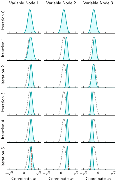
This is a CSS code, where the non-trivial qubit-level stabilizers contain only position operators. The lattice defining the GKP code splits accordingly into momentum and position sectors. Focusing on the position sector, one has a linear decoding graph with three variable nodes and three check nodes. A typical evolution of the messages from the Gaussian mixture implementation (see Appendix C) of the decoder is shown in Fig. 2.

A threshold plot and subthreshold behavior are shown in Fig. 3 using a serial schedule and the list-sphere decoding update rule for the variable nodes with $50$ iterations and a uniform variable-node memory $\gamma=0.15$. While increasing the distance decreases the error rate, the error rate reaches an error floor. Running the local search post-processing routine on $d/2$ positions partially alleviates this issue (not shown), but at increasingly higher decoding complexity.

One might find the above result surprising following the usual intuition that message-passing on a tree is exact and thus should work for this example without issues. However, this argument is too simple as we are not implementing the exact message-passing algorithm described in Section II.1.2, but instead have implemented variable node updates approximately within the Gaussian mixture framework, see Appendix C. Indeed, in the classical literature on low-density lattice codes, the case of low degree graphs is typically omitted and convergence is only proven in the, more relevant, case of higher degree magic-square LDLC, see, e.g., Ref. [36].

In Figure 4 we show the logical error rate performance of the repetition code using our implementation of the quantized decoder of Sommer et al., see Appendix B, with a resolution $\Delta=1/32$ over $L=256$ quantization bins. Compared to the Gaussian mixture decoder implementation, the quantized decoder implementation shows a higher threshold and has an error floor that is independent of the noise rate $\sigma$ which only becomes apparent at low error rates and high distances, see also Figure 4(b). In Figure 5 we show that the error floor in the quantized decoder is again due to the approximate nature of the decoder and it can be removed by increasing the resolution (lower $\Delta$) in the decoder. Alternatively, post-processing methods can be employed to reduce the error floor.

As an example to showcase the performance of the decoder on quantum codes with larger graph degree, we consider small instances of Hamming-based generalized bicycle codes [40], also known as simplex codes [51]. Figure 6 shows the logical $X$ error rate of the $\llbracket 30,8,4\rrbracket$, $\llbracket 62,10,6\rrbracket$, and $\llbracket 126,12,10\rrbracket$ codes subject to the code capacity noise model characterized by the noise strength $\sigma$. The performance is achieved by running 50 iterations of the decoder, using a serial update schedule, and using a list-sphere decoding updating schedule for the variable nodes. We also employ memory $\gamma=0.15$ in the update rules for increased performance, see Appendix C.1. For these instances, no post-processing is applied, demonstrating the good convergence properties of the decoder for the right set of codes. Notably, the threshold of the code and decoder combination is not significantly behind that of concatenated surface codes [35].

References

- [1] (2015) Solving the closest vector problem in time—the discrete Gaussian strikes again!. In 2015 IEEE 56th Annual Symposium on Foundations of Computer Science (FOCS), pp. 563–582. External Links: 1504.01995, Document, Link Cited by: §I.
- [2] (2025) Scaling and networking a modular photonic quantum computer. Nature 638 (8052), pp. 912–919. External Links: ISSN 1476-4687, Document, Link Cited by: §I.
- [3] (2002) Closest point search in lattices. IEEE Trans. Inf. Th. 48 (8), pp. 2201–2214. External Links: ISSN 1557-9654, Document Cited by: §C.1.1, §II.1.3, §IV.1.
- [4] (2002) Sampling short lattice vectors and the closest lattice vector problem. In Proceedings of the 17th Annual IEEE Conference on Computational Complexity (CCC 2002), pp. 53–57. External Links: Document, Link Cited by: §II.1.2.
- [5] (1993) The hardness of approximate optima in lattices, codes, and systems of linear equations. In Proceedings of 1993 IEEE 34th Annual Foundations of Computer Science, pp. 724–733. External Links: Document, Link Cited by: §I, §II.1.2.
- [6] (2026) SymplecticGKP.jl. GitHub. External Links: Link Cited by: Appendix E, §III.2.
- [7] (1986) On Lovász’ lattice reduction and the nearest lattice point problem. Combinatorica 6 (1), pp. 1–13. External Links: ISSN 1439-6912, Document, Link Cited by: §II.1.2, §IV.1.
- [8] (2024) Analog information decoding of bosonic quantum low-density parity-check codes. PRX Quantum 5 (2), pp. 020349. External Links: 2311.01328, Document, Link Cited by: §I.
- [9] (2021) Blueprint for a scalable photonic fault-tolerant quantum computer. Quantum 5, pp. 392. External Links: 2010.02905, Document, Link Cited by: §I.
- [10] (2024) Advances in bosonic quantum error correction with Gottesman–Kitaev–Preskill codes: Theory, engineering and applications. Progr. Quant. Elect. 93, pp. 100496. External Links: 2308.02913, ISSN 0079-6727, Document, Link Cited by: §I.
- [11] (2025) Fiber bundle fault tolerance of GKP codes. Quantum 9, pp. 1899. External Links: Document, Link, ISSN 2521-327X, 2410.07332 Cited by: Appendix E, §III.2.
- [12] (2020) Quantum error correction of a qubit encoded in grid states of an oscillator. Nature 584 (7821), pp. 368–372. External Links: 1907.12487, ISSN 1476-4687, Document, Link Cited by: §I.
- [13] (2017) Roads towards fault-tolerant universal quantum computation. Nature 549 (7671), pp. 172–179. External Links: 1612.07330, ISSN 1476-4687, Document, Link Cited by: §I.
- [14] (2022) Gottesman-Kitaev-Preskill codes: A lattice perspective. Quantum 6, pp. 648. External Links: 2109.14645, Document, Link Cited by: §I, §II.3, §II.3, §II.3, §II.3, §II.3, §II.3, §II.3, §II.4, §III.2, §III.3, §III.4.
- [15] (2024) Good Gottesman-Kitaev-Preskill codes from the NTRU cryptosystem. Quantum 8, pp. 1398. External Links: Document, Link, 2303.02432 Cited by: §I.
- [16] (2024) The fabulous world of GKP codes. Ph.D. Thesis, Freie Universität Berlin. External Links: 2412.02442, Document, Link Cited by: §III.3.
- [17] S. S. Chern, B. Eckmann, P. de la Harpe, H. Hironaka, F. Hirzebruch, N. Hitchin, L. Hörmander, M.-A. Knus, A. Kupiainen, J. Lannes, G. Lebeau, M. Ratner, D. Serre, Ya. G. Sinai, N. J. A. Sloane, J. Tits, M. Waldschmidt, S. Watanabe, M. Berger, J. Coates, and S. R. S. Varadhan (Eds.) (1999) Sphere packings, lattices and groups. Grundlehren Der Mathematischen Wissenschaften, Vol. 290, Springer, New York, NY. External Links: Document, Link, ISBN 978-1-4757-6568-7 Cited by: §III.4.
- [18] (2003) Approximating CVP to within almost-polynomial factors is NP-hard. Combinatorica 23 (2), pp. 205–243. External Links: ISSN 1439-6912, Document, Link Cited by: §II.1.2.
- [19] (2025) Mind the gaps: the fraught road to quantum advantage. External Links: 2510.19928, Document, Link Cited by: §I, §I.
- [20] (2019) Encoding a qubit in a trapped-ion mechanical oscillator. Nature 566 (7745), pp. 513–517. External Links: 1807.01033, ISSN 1476-4687, Document, Link Cited by: §I.
- [21] (1995) Soft-decision decoding of linear block codes based on ordered statistics. IEEE Trans. Inf. Th. 41 (5), pp. 1379–1396. External Links: ISSN 1557-9654, Document Cited by: §IV.1.
- [22] (2018) High-threshold fault-tolerant quantum computation with analog quantum error correction. Phys. Rev. X 8 (2), pp. 021054. External Links: 1712.00294, Document, Link Cited by: §I.
- [23] (1960) Low density parity check codes. Thesis, Massachusetts Institute of Technology. External Links: Link Cited by: §II.1.2.
- [24] (1999) Approximating shortest lattice vectors is not harder than approximating closest lattice vectors. Inf. Proc. Lett. 71 (2), pp. 55–61. External Links: ISSN 0020-0190, Document, Link Cited by: §I, §II.1.2.
- [25] (2001) Encoding a qubit in an oscillator. Phys. Rev. A 64 (1), pp. 012310. External Links: quant-ph/0008040, ISSN 1050-2947, Document, Link Cited by: §I, §II.3, §II.3, §II.3, §III.2.
- [26] (2020) Enhanced noise resilience of the surface–Gottesman-Kitaev-Preskill code via designed bias. Phys. Rev. A 102 (5), pp. 052408. External Links: 2004.00541, Document, Link Cited by: §I.
- [27] (2001) Achievable rates for the Gaussian quantum channel. Phys. Rev. A 64 (6), pp. 062301. External Links: quant-ph/0105058, Document, Link Cited by: §I.
- [28] (2022) Protocol for generating optical Gottesman–Kitaev–Preskill states with cavity QED. Phys. Rev. Lett. 128 (17), pp. 170503. External Links: 2104.07981, Document, Link Cited by: §I.
- [29] (2026) LatticeDecoder.jl. GitHub. External Links: Link Cited by: §II.1.3.
- [30] (2024) Logical states for fault-tolerant quantum computation with propagating light. Science 383 (6680), pp. 289–293. External Links: 2309.02306, Document, Link Cited by: §I.
- [31] (2008) Message-passing decoding of lattices using Gaussian mixtures. In 2008 IEEE International Symposium on Information Theory, pp. 2489–2493. External Links: 0802.0554, ISSN 2157-8117, Document Cited by: Appendix C, Appendix C, Appendix C, §II.1.3.
- [32] (2009) Single-Gaussian messages and noise thresholds for decoding low-density lattice codes. In 2009 IEEE International Symposium on Information Theory, Seoul, South Korea, pp. 734–738. External Links: Document, Link, ISBN 978-1-4244-4312-3 Cited by: Appendix C.
- [33] (1982) Factoring polynomials with rational coefficients. Math. Ann. 261 (4), pp. 515–534. External Links: ISSN 1432-1807, Document, Link Cited by: §IV.1.
- [34] (2015) Construction of structured low density lattice codes based on finite fields. In 2015 IEEE Symposium on Computers and Communication (ISCC), pp. 643–648. External Links: Document, Link Cited by: §II.1.1.
- [35] (2023) Closest lattice point decoding for multimode Gottesman-Kitaev-Preskill codes. PRX Quantum 4 (4), pp. 040334. External Links: 2303.04702, Document, Link Cited by: §I, §II.3, §II.3, §II.4, §IV.3.
- [36] (2019) Efficient decoding of low density lattice codes. IEEE Wire. Comm. Lett. 8 (4), pp. 1195–1199. External Links: 1806.05524, ISSN 2162-2345, Document Cited by: §C.1.2, Appendix C, Appendix C, §IV.2.
- [37] (2002) Complexity of lattice problems: a cryptographic perspective. The Springer International Series in Engineering and Computer Science, Vol. 671, Springer, Boston, MA. External Links: ISBN 978-0-7923-7688-0, Document, Link Cited by: §II.1.2.
- [38] (2022) Low-overhead fault-tolerant quantum error correction with the surface-GKP code. PRX Quantum 3 (1), pp. 010315. External Links: 2103.06994, Document, Link Cited by: §I.
- [39] (2020) Fault-tolerant bosonic quantum error correction with the surface–Gottesman-Kitaev-Preskill code. Phys. Rev. A 101 (1), pp. 012316. External Links: 1908.03579, Document, Link Cited by: §I.
- [40] (2021) Degenerate quantum LDPC codes with good finite length performance. Quantum 5, pp. 585. External Links: 1904.02703, Document, Link Cited by: §IV.3, §IV.
- [41] (2002) Probability, random variables, and stochastic processes. 4th ed edition, McGraw-Hill Series in Electrical and Computer Engineering, McGraw-Hill, Boston. External Links: Link, ISBN 978-0-07-366011-0 Cited by: §II.1.2.
- [42] (1994) On coding without restrictions for the AWGN channel. IEEE Trans. Inf. Th. 40 (2), pp. 409–417. External Links: ISSN 1557-9654, Document, Link Cited by: §II.2.
- [43] (2022) Finite Rate QLDPC-GKP coding scheme that surpasses the CSS Hamming bound. Quantum 6, pp. 767. External Links: 2111.07029, Document, Link Cited by: §I.
- [44] (2019) Quantum error correction: an introductory guide. Contemp. Phys. 60 (3), pp. 226–245. External Links: 1907.11157, Document, Link Cited by: §I.
- [45] (1948) A mathematical theory of communication. The Bell Syst. Tech. J. 27 (3), pp. 379–423. External Links: ISSN 0005-8580, Document, Link Cited by: §II.2.
- [46] (2007) Low density lattice codes. External Links: 0704.1317, Link Cited by: Appendix B, §C.1.1, §I, §II.1.1, §II.1.1, §II.1.2, §II.1.2, §II.1.2, §II.1.2, Theorem II.1, §III.1, §VI, Definition 1, 3.
- [47] (2026) Qudit low-density parity-check codes. Quantum 10, pp. 2023. External Links: Document, Link, ISSN 2521-327X, 2510.06495 Cited by: §III.4.
- [48] (2015) Quantum error correction for quantum memories. Rev. Mod. Phys. 87 (2), pp. 307–346. External Links: 1302.3428, Document, Link Cited by: §I.
- [49] (2019) Quantum error correction with the toric Gottesman-Kitaev-Preskill code. Phys. Rev. A 99 (3), pp. 032344. External Links: 1810.00047, Document, Link Cited by: §I.
- [50] (2023) Efficient decoder design for low-density lattice codes from the lattice viewpoint. IEEE Open J. Commun. Soc. 4, pp. 1839–1854. External Links: ISSN 2644-125X, Document, Link Cited by: §C.1.1, §C.1.1, Appendix C, Appendix C, §II.1.3.
- [51] (2025) Explicit construction of low-overhead gadgets for gates on quantum LDPC codes. arXiv. External Links: 2511.15989, Document, Link Cited by: Figure 6, §IV.3, §IV.
- [52] (2020) Realizing modular quadrature measurements via a tunable photon-pressure coupling in circuit QED. Phys. Rev. A 101 (5), pp. 053840. External Links: 1909.10075, Document, Link Cited by: §I.
- [53] (2016) An efficient algorithm for optimally solving a shortest vector problem in compute-and-forward design. IEEE Trans. Wire. Comm. 15 (10), pp. 6541–6555. External Links: 1410.4278, ISSN 1558-2248, Document Cited by: §C.1.1.
- [54] (1950) The theory of groups and quantum mechanics. Dover Books on Mathematics, Dover Publications, New York. External Links: ISBN 978-0-486-60269-1 Cited by: §II.3.
- [55] (2023) Qubit-oscillator concatenated codes: Decoding formalism and code comparison. PRX Quantum 4 (2), pp. 020342. External Links: 2209.04573, Document, Link Cited by: §I.