Learning CNN Filters via Generalized Stein’s Method

The index model is a classical statistical method which generalizes the linear regression to a nonlinear format from a different perspective than neural networks. Specifically, a multi-index model (MIM) usually takes the form of $\mathbb{E}(y|\boldsymbol{x})=f(\boldsymbol{x}^{\top}\boldsymbol{b}_{1},\ldots,\boldsymbol{x}^{\top}\boldsymbol{b}_{R})$, where $\boldsymbol{b}_{1},\ldots,\boldsymbol{b}_{R}$ are the target index vectors, and $f$ is an unknown multi-variate nonlinear function, also known as the link function. When $R=1$, the MIM reduces to the single index model (SIM), which leads to the index $\boldsymbol{x}^{\top}\boldsymbol{b}$ and the function $f$ being univariate. Index models not only offer considerable adaptability by incorporating the nonlinear link function, but also avoid the curse of dimensionality by representing the outcome through a low-dimensional representation of the input. A classical line of research on index models is closely connected to sufficient dimension reduction, among which sliced inverse regression (SIR) (Li, 1991) is one of the most influential approaches. This framework has inspired a large body of extensions, including sliced average variance estimation (Cook and Weisberg, 1991, SAVE;), and tensor-valued extensions such as TensorSIR (Ding and Cook, 2015). However, these methods typically rely on relatively strong probabilistic assumptions, such as the linearity condition and constant variance condition, which are often satisfied only under elliptical or Gaussian-type distributions.

Another line of research on learning index models is motivated by the classical Stein’s identity (Stein, 1981), which implies that, in the simplest setting where $\boldsymbol{x}$ follows a standard Gaussian distribution, the index vector $\boldsymbol{b}$ is proportional to $\mathbb{E}(\boldsymbol{x}\cdot y)$, regardless of the unknown link function $f$. Early works along this direction include average derivative estimation (Stoker, 1986, ADE;) and principal Hessian directions (Li, 1992, PHD;). More recently, Stein-based methods have been revisited and substantially extended to more general settings. For instance, Plan and Vershynin (2016) and Plan et al. (2017) considered SIM with sparse index vectors, and Balasubramanian et al. (2025) extended the framework to functional regression. Yang et al. (2017) and Goldstein et al. (2018) generalized the Gaussian input assumption to heavy-tailed or non-Gaussian scenarios, and Fan et al. (2023) studied implicit regularization in SIM. Nevertheless, most existing works are developed under relatively simple and idealized settings, typically focusing on SIM with vector-valued inputs and assuming that the input distribution is known. As a result, they provide limited practical guidance for handling complex real-world data such as imaging data.

The rest of the paper is organized as follows. Section 2 introduces the ADNI dataset in detail. Section 3 establishes the connections between CNNs and index models, and present our SVD-based estimation. Section 4 provide theoretical analyses for estimating filters under different settings. Section 5 presents the ADNI data analysis, and Section 6 includes comprehensive simulation studies. Finally, Section 7 concludes with further discussions.

Notations. We use bold uppercase letters $\boldsymbol{A}$, $\boldsymbol{B}$ to denote matrices, bold lowercase letters $\boldsymbol{a}$, $\boldsymbol{b}$ to denote vectors. We let $\text{vec}(\cdot)$ be the vectorization operator and $\text{vec}^{-1}_{(\cdot)}(\cdot)$ be its inverse with the subscripts indicating the matrix size. For a vector ${\bf v}$, $\|{\bf v}\|_{q}=(\sum_{j}|v_{j}|^{q})^{1/q}$ is the $\ell_{q}$ norm. For a matrix $\boldsymbol{A}$, $\|\boldsymbol{A}\|_{F}=\sqrt{\sum_{i,j}\boldsymbol{A}_{i,j}^{2}}$ is the Frobenius norm, $\lambda_{min}(\boldsymbol{A})$ is the minimum eigenvalue of matrix $\boldsymbol{A}$. Moreover, we let $\langle\cdot,\cdot\rangle$ to denote the inner product. In addition, given two sequences $\{x_{n}\}$ and $\{y_{n}\}$, we denote $x_{n}=\mathcal{O}(y_{n})$ if $|x_{n}|\leq C_{1}|y_{n}|$ for some absolute constant $C_{1}$ and denote $x_{n}=\Omega(y_{n})$ if $|x_{n}|\geq C_{2}|y_{n}|$ for some absolute constant $C_{2}$.

Let $\boldsymbol{X}^{\text{ori}}\in\mathbb{R}^{P_{1}\times P_{2}}$ denote the original matrix-valued input, such as raw image data. In a typical convolutional neural network, the raw image usually first goes through a convolutional layer, and then proceeds to pooling and fully connected layers. We shall focus on the first convolutional layer and denote $\boldsymbol{B}_{1},\ldots,\boldsymbol{B}_{R}\in\mathbb{R}^{d_{1}\times d_{2}}$ as $R$ convolution filters in the first layer of a CNN. Then, the output of a convolutional neural network can be written as the following form

Here $\star$ is a convolution operator to be discussed in detail later, $\sigma(\cdot)$ is a component-wise nonlinear activation function, such as ReLU (Rectified Linear Unit) or Sigmoid function. Furthermore, the multivariate function $g$ incorporates the remaining structure of CNN, including pooling layers, fully-connected layers, and other components in a CNN. If we further combine $g$ with the activation function $\sigma$, the CNN output (1) can be written as

We now turn our attention to the convolution operator $\star$. We shall first consider a non-overlapping convolution, further extensions to its overlapping version will be discussed later. Given any matrix $\boldsymbol{M}\in\mathbb{R}^{P_{1}\times P_{2}}$ and a filter $\boldsymbol{B}\in\mathbb{R}^{d_{1}\times d_{2}}$, where $d_{1},d_{2}$ are factors of $P_{1},P_{2}$ respectively, the non-overlapping convolution is defined as

Here, $(p_{1},p_{2})=(P_{1}/d_{1},P_{2}/d_{2})$ and $\boldsymbol{M}_{j,k}^{d_{1},d_{2}}$ represents the $(j,k)$-th block of size $d_{1}\times d_{2}$ in $\boldsymbol{M}$ for $1\leq j\leq p_{1}$ and $\ 1\leq k\leq p_{2}$. With deep learning language, the stride size is set equal to the filter size under non-overlapping scenario. The convolution operation aims to extract feature information, thereby enhancing prediction in the subsequent layers. While through the non-overlapping design, dimension reduction can be achieved. Notably, the non-overlapping convolution, being the simplest case, has been extensively studied in the literature, for example, Brutzkus and Globerson (2017); Du et al. (2018); Cao and Gu (2019); Feng and Yang (2024). Let $p=p_{1}p_{2}$ be the total number of non-overlapping blocks and $d=d_{1}d_{2}$ be the number of elements in each block.

Now we consider a matrix reshaping operator that allows us to further connect the CNN and index models. Given any matrix $\boldsymbol{M}\in\mathbb{R}^{P_{1}\times P_{2}}$, the operator $\mathcal{R}_{(d_{1},d_{2})}:\mathbb{R}^{P_{1}\times P_{2}}\rightarrow\mathbb{R}^{p\times d}$ is defined as a mapping from $\boldsymbol{M}$ to

A key property holds for $\boldsymbol{X}^{\text{ori}}\in\mathbb{R}^{P_{1}\times P_{2}}$ and $\boldsymbol{B}\in\mathbb{R}^{d_{1}\times d_{2}}$ that

Figure 1 illustrates the transformation of convolution operation into matrix multiplication through the operator $\mathcal{R}_{(d_{1},d_{2})}(\cdot)$.

Let $\boldsymbol{X}=\mathcal{R}_{(d_{1},d_{2})}(\boldsymbol{X}^{\text{ori}})\in\mathbb{R}^{p\times d}$ be the reshaped input and $\boldsymbol{b}_{r}=\text{vec}(\boldsymbol{B}_{r})\in\mathbb{R}^{d}$ for $r=1,\ldots,R$. Then we can rewrite (2) as

With a slight abuse of notation, we also use the same function notation $f$ in (5). However, we shall note that the $f$ in (5) is not identical to that in (2) as the inputs were reshaped. If we model certain outcome $Y$ through the above formulation, we have

Model (6) clearly bears a resemblance to an MIM, although in fact they are different. In a standard MIM, the input is typically a vector, so each index is a scalar. In model (6), however, $\boldsymbol{X}$ is a matrix of dimension $p\times d$, which makes each index $\boldsymbol{X}\boldsymbol{b}_{r}$ a $p$-dimensional vector. Consequently, the function in (6) is a more general function with an input dimension $p\times R$. Let $\boldsymbol{\Theta}=\left(\boldsymbol{b}_{1},\ldots,\boldsymbol{b}_{R}\right)\in\mathbb{R}^{d\times R}$ denote the collection of convolutional filters. Then model (6) can be compactly written as $\mathbb{E}(Y|\boldsymbol{X})=f(\boldsymbol{X}\boldsymbol{\Theta})$.

Based on model (6), we assume the relationship between $Y$ and $\boldsymbol{X}$ is $Y=f(\boldsymbol{X}\boldsymbol{\Theta})+\epsilon$, where the noise term $\epsilon$ is independent of $\boldsymbol{X}$. We assume that $\epsilon$ is centered and sub-Gaussian, i.e. $\mathbb{E}[\epsilon]=0$ and $\mathbb{E}[|\epsilon|^{k}]^{\frac{1}{k}}\leq\sigma\sqrt{k}$ for all $k\in\mathbb{N}$ and an absolute constant $\sigma>0$. Let $\boldsymbol{X}_{i}=\mathcal{R}_{(d_{1},d_{2})}(\boldsymbol{X}_{i}^{\text{ori}})\in\mathbb{R}^{p\times d}$ and $Y_{i}\in\mathbb{R}$ for $i\in[n]$ be $n$ i.i.d. observations that follow $Y_{i}=f(\boldsymbol{X}_{i}\boldsymbol{\Theta})+\epsilon_{i}$. Similar to index models, $\boldsymbol{\Theta}$ is not identifiable when $f$ is unknown. Specifically, it is identifiable only up to an invertible linear transformation, since any such transformation can be absorbed into $f$. Therefore, our goal is to learn the column space in $\boldsymbol{\Theta}$ based on a generalized version of Stein’s identity. To get started, we shall first define the score function associated with the input $\boldsymbol{X}$.

Then we have the following generalized version of first-order Stein’s identity.

Lemma 3.2 serves as the basis for our estimation of $\boldsymbol{\Theta}$. It shows that provided $\mathbb{E}[YS(\boldsymbol{X})]$ has rank $R$, the column space of $\boldsymbol{\Theta}$ can be determined by the top $R$ right singular vectors of $\mathbb{E}[YS(\boldsymbol{X})]$. With the sample version $(1/n)\sum_{i=1}^{n}Y_{i}S(\boldsymbol{X}_{i})$ being a natural estimate for $\mathbb{E}[YS(\boldsymbol{X})]$, we propose the following SVD based estimation for $\boldsymbol{\Theta}$,

where $\mathrm{SVD}_{v,R}(\boldsymbol{M})$ refers to the top $R$ right singular vectors of a matrix $\boldsymbol{M}$.

We emphasize that this method is general as it applies to arbitrary distribution of input $\boldsymbol{X}$, provided that the score $S(\boldsymbol{X})$ is known or well estimated. Moreover, this estimator does not rely on the link function $f$, therefore regardless of the complexity of subsequent pooling or fully connected layers in a CNN. Based on SVD, the proposed estimator aims to learn a compact set of informative convolutional directions rather than to reproduce every possibly redundant filter in a large CNN. This is consistent with empirical observations that CNNs often learn filters with substantial redundancy (Jaderberg et al., 2014; Wang et al., 2020). Therefore, the orthogonality of $\hat{\boldsymbol{\Theta}}$ should be regarded as a basis-recovery feature of the estimator, rather than as a structural assumption on all practical CNN filters.

Although the method is introduced to estimate filters in the first convolutional layer, in practice it serves as a representation learning method that efficiently extracts convolutional features without training the full CNN. The resulting convolutional features can then be used in downstream tasks and integrated with either statistical models or neural networks. Specifically, an applied researcher can use this method following steps below.

• Step 1.

  Estimate the score function. Under a suitable parametric model for the input distribution, the score can be estimated by plug-in estimators. For example, under a Gaussian model, the empirical mean and covariance give an explicit estimate of the score function, as described in Section 4.3.

• Step 2.

  Estimate filters. Compute $(1/n)\sum_{i=1}^{n}Y_{i}\hat{S}(\boldsymbol{X}_{i})$ and perform SVD. The top right singular vectors form $\hat{\boldsymbol{\Theta}}$, and each column is reshaped into a convolutional filter $\hat{\boldsymbol{B}}_{r}=\mathrm{vec}^{-1}_{(d_{1},d_{2})}(\hat{\boldsymbol{\Theta}}_{[:,r]})$.

• Step 3.

  Construct representations and fit downstream models. Apply the estimated filters to the original images to obtain convolutional feature maps, and then use these features in a downstream model such as linear regression, LASSO, FCN, or CNN.

A notable advantage of the proposed method is its seamless integration with downstream statistical models, as the extracted features can be directly used as their inputs. This enables a natural combination of the representation power of CNN-based feature extraction with the strengths of classical statistical methods, including interpretability and inference. We also note that if the input distribution is completely unknown and no suitable parametric model is available, score estimation becomes a substantive problem. In such cases, nonparametric score estimation methods, such as Zhou et al. (2020), may provide an alternative, but their accuracy should be checked for the application at hand.

Under heavy-tailed data, the straightforward sample version $(1/n)\sum_{i=1}^{n}Y_{i}S(\boldsymbol{X}_{i})$ may not be an optimal estimate for $\mathbb{E}[YS(\boldsymbol{X})]$ due to a lack of concentration. In fact, not only can the input $\boldsymbol{X}$ be heavy-tailed, but the outcome $Y$ or the score function $S(\boldsymbol{X})$ could also exhibit heavy-tail behavior due to the unknown link function $f$. These issues have been discussed in the literature, where the truncation argument has been proposed, as seen in works such as Catoni (2012); Minsker (2018); Yang et al. (2017). We adopt similar strategies and propose an improved estimator of the truncated form.

We begin by introducing a class of non-decreasing functions $\phi:\mathbb{R}\rightarrow\mathbb{R}$ satisfying

A straightforward function satisfying the upper and lower exponential-type bounds is

It is a convenient choice as it attains these bounds tightly and modifies the original estimator only as much as needed to control extreme values, while other truncation functions with the same bounding properties could also be used. Figure 2 illustrates the function $\phi$.

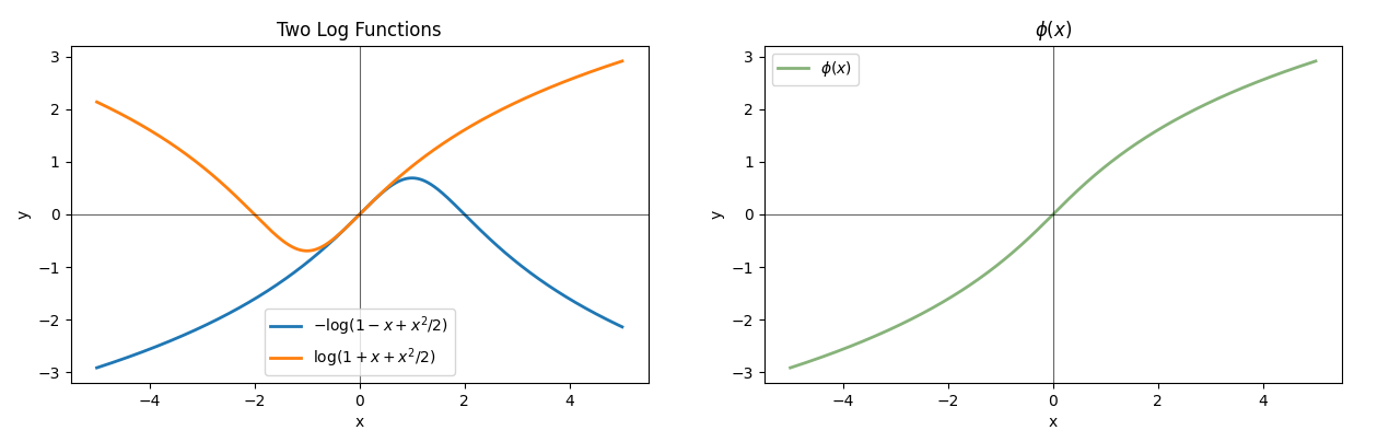
We introduce a linear mapping $\psi:\mathbb{R}^{p\times d}\rightarrow\mathbb{R}^{p\times d}$ based on the non-decreasing function $\phi$. For a given matrix $\boldsymbol{X}\in\mathbb{R}^{p\times d}$, consider the spectral decomposition of its Hermitian dilation:

Further, define $\tilde{\boldsymbol{X}}=\boldsymbol{U}(\phi\circ\boldsymbol{\Sigma})\boldsymbol{U}^{\top}$ and write it into block form as

where $\phi\circ\boldsymbol{\Sigma}$ indicates that the function $\phi$ is applied element-wise on $\boldsymbol{\Sigma}$. Then we define $\psi(\boldsymbol{X})=\tilde{\boldsymbol{X}}_{12}$. Based on $\psi$, we introduce a new estimator $\tilde{\boldsymbol{\Theta}}$ for $\boldsymbol{\Theta}$ with a truncated form

where $\tau\left(Y_{i}S(\boldsymbol{X}_{i})\right)=1/\theta\cdot\psi\left[\theta Y_{i}S(\boldsymbol{X}_{i})\right]$, and $\theta>0$ is a thresholding parameter. In later analysis, we will provide theoretical analyses of $\tilde{\boldsymbol{\Theta}}$ and demonstrate its advantages over $\hat{\boldsymbol{\Theta}}$ in (8) under heavy-tailed distributions.

In this section, we provide theoretical guarantees for estimating $\boldsymbol{\Theta}$ with a single convolution filter. With $R=1$, we let $\boldsymbol{b}=\text{vec}(\boldsymbol{B})=\boldsymbol{\Theta}\in\mathbb{R}^{d}$ be the target filter and denote the original and truncated version of the estimated filter as $\hat{\boldsymbol{b}}=\hat{\boldsymbol{\Theta}}$ and $\tilde{\boldsymbol{b}}=\tilde{\boldsymbol{\Theta}}$, respectively. We assume that $\|\boldsymbol{b}\|_{2}=1$ to avoid identifiability issues. We first consider the original estimator $\hat{\boldsymbol{b}}$ under sub-Gaussian input. To get started, we present necessary conditions below.

Assumption 1 requires that each entry of the score function $S(\boldsymbol{X})$ is sub-Gaussian. Such an assumption is rather mild and can be satisfied by a wide range of random distributions. For example, when $\boldsymbol{X}$ follows a Gaussian distribution with entries $X_{jk}\sim N(\mu_{jk},\sigma_{jk}^{2})$, it results in $S_{jk}(\boldsymbol{X})=(X_{jk}-\mu_{jk})/\sigma_{jk}^{2}$ also being a Gaussian random variable, which is clearly sub-Gaussian. Moreover, when $X_{jk}$ follows a heavier tailed Students’ $t$ distribution, it can be easily verified that the score is bounded and inherently sub-Gaussian. This implies that even if the input $\boldsymbol{X}$ is not sub-Gaussian, the score could still potentially be sub-Gaussian.

Assumption 2 requires that $f(\boldsymbol{X}\boldsymbol{\Theta})$ is a sub-Gaussian random variable. This assumption is relatively mild. Clearly, Assumption 2 automatically holds when $f\in\mathbb{R}^{p\times R}\mapsto\mathbb{R}$ is a bounded function. Moreover, when $f$ is Lipschitz continuous and $\boldsymbol{X}$ is sub-Gaussian, it is easy to show that Assumption 2 could also be satisfied.

In Assumption 3, we assume that the derivative of the non-linear function $f$ at $\boldsymbol{Z}=\boldsymbol{X}\boldsymbol{b}$ maintains a constant level. This assumption ensures identifiability by requiring that the function value $f(\boldsymbol{X}\boldsymbol{b})$ is adequately sensitive to perturbations around the true value $\boldsymbol{b}$. This assumption is mild, as it merely assumes a constant scale of the derivatives in expectation. In practice, the assumption can be evaluated by inspecting the empirical singular value spectrum of the matrix $\frac{1}{n}\sum_{i=1}^{n}Y_{i}S(\boldsymbol{X}_{i})$, which is supported when the leading singular value is significantly larger than the remaining spectrum, illustrated in the Supplementary Material.

Theorem 4.1 suggests that the $\ell_{2}$-convergence rate of $\hat{\boldsymbol{b}}$ is $\mathcal{O}\left(\sqrt{d\log(pd)/n}\right)$ under the sub-Gaussian setting. This rate is optimal up to a logarithmic factor. In fact, consider the simplest scenario where $f$ is linear, meaning that $\mathbb{E}(Y_{i}|\boldsymbol{X}_{i})=\boldsymbol{c}^{\top}\boldsymbol{X}_{i}\boldsymbol{b}$, with $\boldsymbol{c}\in\mathbb{R}^{p}$ being a known vector. In this case, the $\ell_{2}$-convergence rate of an OLS estimate of $\boldsymbol{b}$, denoted as $\hat{\boldsymbol{b}}^{ols}$, is $\mathcal{O}\left(\sqrt{d/n}\right)$. Our rate in Theorem 4.1 matches with this OLS rate apart from a logarithmic factor, which confirms the optimality of (12).

Now we focus on the truncated estimator, for which we can provide sharp error bounds even when both the outcomes and the scores exhibit heavy-tailed behavior.

Assumption 4 relaxed the sub-Gaussian Assumption 1 to a bounded fourth-moment assumption on the outcome $Y$ and the score $S(\boldsymbol{X})$. Under this assumption, heavy-tailed inputs could be included. We note that similar assumptions have been studied in the literature, such as Yang et al. (2017); Fan et al. (2018); Fan et al. (2021); Fan et al. (2023). With the bounded moment assumption, we can present the theoretical results for the truncated estimator.

By Theorem 4.2, the truncated estimator could achieve a convergence rate of $\mathcal{O}\left(\sqrt{d\log(p+d)/n}\right)$ with a carefully chosen truncation parameter $\theta$. In other words, even if both the outcome $Y_{i}$ and the score $S(\boldsymbol{X}_{i})$ are heavy-tailed, a nearly optimal convergence rate could still be guaranteed under a bounded moment condition. On the other hand, it is worth noting that the bounded expectation assumption on $f$, referred to as Assumption 2, is not necessary in Theorem 4.2. In other words, the convergence can be guaranteed solely under the constant derivatives Assumption 3 and the bounded scores assumption 4.

In this section, we consider general cases with $R\geq 2$ filters in CNNs. Similar to Section 4.1, we study both the original and truncated versions of the estimator under sub-Gaussian and moment conditions, respectively. However, as previously discussed, when $R\geq 2$, $\boldsymbol{\Theta}$ is not identifiable with an unknown link function $f$. Thus, our goal is to learn the column space of $\boldsymbol{\Theta}$ and prove the convergence of the estimators using the following distance measure

where $\mathbb{H}_{R}$ is the set of $R\times R$ orthogonal matrices. It is worth noting that when $R=1$, the column space distance $\text{dist}\left(\boldsymbol{b},\hat{\boldsymbol{b}}\right)$ reduces to the vector distance $\|\hat{\boldsymbol{b}}-\boldsymbol{b}\|_{2}$ when $\|\boldsymbol{b}\|_{2}=\|\hat{\boldsymbol{b}}\|_{2}$.

In a multi-filter setting, we require assumptions similar to those used for single-filter estimation, with Assumption 3 replaced by Assumption 5 below.

Assumption 5 imposes a lower bound of the non-zero singular values of $\mathbb{E}[Y_{i}S(\boldsymbol{X}_{i})]$. This assumption can be viewed as an extension of Assumption 3 in a multiple filters scenario. For example, when each entry of $\mathbb{E}[\nabla_{\boldsymbol{Z}}f(\boldsymbol{X}\boldsymbol{\Theta})]$ is $\Omega(1/\sqrt{R})$ and the columns of $\mathbb{E}[\nabla_{\boldsymbol{Z}}f(\boldsymbol{X}\boldsymbol{\Theta})]$ are nearly orthogonal, it is easy to show that all the $R$ non-zero singular values of $\mathbb{E}[YS(\boldsymbol{X})]$ have a lower bound in scale of $\Omega(\sqrt{p/R})$. Similarly, in practice it can be also assessed by inspecting the empirical singular value spectrum of $\frac{1}{n}\sum_{i=1}^{n}Y_{i}S(\boldsymbol{X}_{i})$, which is supported when the leading $R$ singular values are clearly separated from the remaining spectrum.

In this multiple filters case, we achieve a convergence rate of $\mathcal{O}\left(\sqrt{Rd\log(pd)/n}\right)$ under the sub-Gaussian assumption. By replacing Assumption 3 with an SVD-type Assumption 5, Theorem 4.3 extends the near-optimal convergence rate stated in Theorem 4.1 to a multiple filter scenario. Moreover, we can eliminate the sub-Gaussian assumptions as detailed below.

We now consider the truncated estimator without imposing the sub-Gaussian assumption. The following theorem extends Theorem 4.2 to the multiple-filter case.

Theorem 4.4 characterizes the convergence rate of the column space of $\tilde{\boldsymbol{\Theta}}$ for multiple filters under the general setting. Compared to Theorem 4.3, Theorem 4.4 further demonstrates that a sharp convergence rate can be guaranteed even when both the outcomes and the scores exhibit heavy-tailed behavior.

To estimate the convolution filters using our approach, a crucial step involves computing the score function, which requires the knowledge of the input distribution. Nevertheless, the input distributions are usually unknown in practice. When the input distribution has a specific parametric form, a natural solution is to use the plug-in estimator. This involves estimating the unknown parameters from the samples and then plugging them into the scores. In this section, we take Gaussian input as an example and demonstrate the convergence of the plug-in estimators.

Let $\boldsymbol{x}_{i}=\text{vec}(\boldsymbol{X}_{i})=\text{vec}\left(\mathcal{R}(\boldsymbol{X}_{i}^{\text{ori}})\right)$ be the vectorized image. Assume that $\boldsymbol{x}_{i}\sim\mathcal{N}(\boldsymbol{\mu},\boldsymbol{\Sigma})$ follows Gaussian distribution with unknown mean $\boldsymbol{\mu}$ and covariance matrix $\boldsymbol{\Sigma}$. Under such a Gaussian case, it is easy to show that the score function reduces to $S(\boldsymbol{X}_{i})=\text{vec}_{(p,d)}^{-1}(\boldsymbol{\Sigma}^{-1}\boldsymbol{x}_{i})$, where $\text{vec}^{-1}_{(p,d)}(\cdot)$ is the inverse operation of transforming a matrix to a vector. Denote the sample mean and sample covariance matrix as $\hat{\boldsymbol{\mu}}=(1/n)\sum_{i=1}^{n}\boldsymbol{x}_{i}$ and $\hat{\boldsymbol{\Sigma}}=(1/n)\sum_{i=1}^{n}\{\boldsymbol{x}_{i}-\hat{\boldsymbol{\mu}}\}\{\boldsymbol{x}_{i}-\hat{\boldsymbol{\mu}}\}^{\top}$, respectively. By plugging the sample mean and sample covariance matrix into the score, we obtain the following estimator:

We now present the following theorem which provides a bound on the column space between $\check{\boldsymbol{\Theta}}$ and the original estimator $\hat{\boldsymbol{\Theta}}$, where the true mean and covariance are used.

Theorem 4.5 shows that column space of the plug-in estimator converges to that of the original estimator at the rate $\mathcal{O}\left(\sqrt{Rd/n}\right)$. In fact, under certain cases, the plug-in estimator may even outperform the original one. To illustrate, consider a natural case where $\boldsymbol{X}_{i}$ follows a zero-mean Gaussian distribution and $f$ is linear, so that $Y_{i}=\langle\boldsymbol{C},\boldsymbol{X}_{i}\boldsymbol{\Theta}\rangle+\varepsilon_{i}$, where $\boldsymbol{C}\in\mathbb{R}^{p\times R}$ is an unknown matrix. This model can be viewed as a low-rank trace regression of the form $\mathbb{E}(Y_{i}|\boldsymbol{X}_{i})=\text{tr}(\boldsymbol{A}\boldsymbol{X}_{i}^{\top})$, where $\boldsymbol{A}=\boldsymbol{C}\boldsymbol{\Theta}^{\top}\in\mathbb{R}^{p\times d}$ is a low-rank matrix. Under this setting, $\check{\boldsymbol{A}}$ in (15) reduces to the OLS estimate of $\boldsymbol{A}$:

As a comparison, the original estimator $\hat{\boldsymbol{A}}$ with true mean and covariance becomes:

By above derivation, $\check{\boldsymbol{A}}$ could potentially provide a better estimation of $\boldsymbol{A}$ in comparison to $\hat{\boldsymbol{A}}$. Particularly, when sample size $n$ is small, $\boldsymbol{\Sigma}^{-1}\hat{\boldsymbol{\Sigma}}$ might deviate from $\boldsymbol{I}$ and then the estimation performance of $\hat{\boldsymbol{A}}$ could be impacted. Consequently, the plug-in estimator $\check{\boldsymbol{\Theta}}$, which consists of the singular vectors of $\check{\boldsymbol{A}}$, might yield a smaller estimation error. This finding is further validated by an extensive simulation study presented in Section 6.3.

We regard MRI images as input $\boldsymbol{X}_{i}^{\text{ori}}$ and generate the responses $Y_{i}$ according to the following models

• (i)

  Single filter: $Y_{i}=f\left(\boldsymbol{X}_{i}^{\text{ori}}\star\boldsymbol{B}\right)+\varepsilon_{i}$.

• (ii)

  Multiple filters with $R=3$: $Y_{i}=f\left(\boldsymbol{X}_{i}^{\text{ori}}\star\boldsymbol{B}_{1},\ \boldsymbol{X}_{i}^{\text{ori}}\star\boldsymbol{B}_{2},\ \boldsymbol{X}_{i}^{\text{ori}}\star\boldsymbol{B}_{3}\right)+\varepsilon_{i}$.

We consider four kinds of link functions $f$ described as (I) to (IV) in Section 6, including linear, nonlinear, fully connected network (FCN) and convolutional neural network (CNN). The filters ($\boldsymbol{B}$; $\boldsymbol{B}_{1}$, $\boldsymbol{B}_{2}$, $\boldsymbol{B}_{3}$) are constructed as the singular vectors of a random matrix followed by reshaped into square matrices of size $4\times 4$, which are fixed throughout all experiments. Consequently, the reshaped images $\boldsymbol{X}_{i}=\mathcal{R}_{(4,4)}(\boldsymbol{X}^{\text{ori}})\in\mathbb{R}^{144\times 16}$. The noise term $\varepsilon_{i}$ is generated as Gaussian distribution $\mathcal{N}(0,\sigma^{2})$ with $\sigma=0.1$.

To validate our approach in real data analysis, a key step involves understanding the distributions of the input. We follow the work of Lindquist (2008) and assume that $\boldsymbol{X}_{i}^{\text{ori}}$ follows a Gaussian distribution with unknown mean and covariance. We implement the plug-in estimator of our approach, and compare with CNNs trained using Adam (Kingma and Ba, 2015), one of the most widely used gradient descent algorithms for training neural networks. We reiterate that our approach does not require the knowledge of link functions while applying Adam necessitates specifying a neural network architecture. To approximate the link functions in a consistent manner, we employ a two-layer fully connected network. Moreover, for the neural network based link functions (FCN and CNN), we additionally include an architecture that matches the true underlying network for generation. Such an “oracle” specification naturally gives Adam an advantage in learning convolutional filters.

We evaluate convolutional filter estimation using the column space distance metric defined in (14). We repeatedly simulate the responses using four of the five folds of the data, and report the average and standard deviation of the estimation errors in Figure 3. As shown in the figure, our method consistently achieves the smallest estimation errors across various link functions in both single and multiple filters scenarios, demonstrating its effectiveness even when the inputs are real MRI images with unknown distributions. Furthermore, these results suggest that Gaussian approximation can be sufficient for the MRI images in this application, providing practical support for the subsequent analysis with real MMSE responses.

We further use real MMSE scores as the response variable. Since the true latent convolutional filters are unknown, direct comparison of estimation accuracy is not feasible. Instead, we evaluate performance from a representation learning perspective by examining predictive performance across different representations and predictive models. That is to say, we consider models of the form $\hat{Y}_{i}=f(h(\boldsymbol{X}^{\text{ori}}))$, where $h$ denotes a representation function and $f$ refers to the downstream predictive model. Specifically, the following representations are included.

• (1)

  Original features: $h(\boldsymbol{X}^{\text{ori}})=\boldsymbol{X}^{\text{ori}}$.

• (2)

  Representations by our method: $h(\boldsymbol{X}^{\text{ori}})=(\boldsymbol{X}^{\text{ori}}\star\boldsymbol{B}_{1},\ldots,\boldsymbol{X}^{\text{ori}}\star\boldsymbol{B}_{R})$, where $\boldsymbol{B}_{r}$ are directly estimated by our method.

• (3)

  Representations by Adam: $h(\boldsymbol{X}^{\text{ori}})=(\boldsymbol{X}^{\text{ori}}\star\boldsymbol{B}_{1},\ldots,\boldsymbol{X}^{\text{ori}}\star\boldsymbol{B}_{R})$, where $\boldsymbol{B}_{r}$ are learned jointly with the full model by Adam.

• (4)

  Representations by TensorSIR: $h(\boldsymbol{X}^{\text{ori}})=\boldsymbol{\Gamma}_{1}^{\top}\boldsymbol{X}^{\text{ori}}\boldsymbol{\Gamma}_{2}$, where $\boldsymbol{\Gamma}_{1}$ and $\boldsymbol{\Gamma}_{2}$ are estimated using tensor-valued sliced inverse regression method proposed by Ding and Cook (2015).

Accordingly, our procedure first estimates filters using the proposed method to obtain convolutional representations, and then trains the predictive models on these representations to perform prediction. For example, when the convolution filters $\boldsymbol{B}_{r}$ are fixed to size $4\times 4$, each convolution operation reduces the input dimension from 2,304 ($=48\times 48$) to 144 ($=12\times 12$). Figure 4 illustrates the filters estimated by our method for $R=3$ along with the corresponding convolutional representations of a sample image. For the gradient-based approach, we adopt the same convolutional architecture as in our method, with the only difference being that the filters are learned jointly with the full model via Adam. As a result, the two types of representations have the same dimensions given the same $R$. TensorSIR is an extension of sliced inverse regression for tensor-valued inputs and is therefore naturally applicable to matrix-valued imaging data. In this setting, $\boldsymbol{\Gamma}_{1}$ and $\boldsymbol{\Gamma}_{2}$ are estimated to perform two-way dimension reduction along the row and column directions, respectively.

Based on the above representations, we consider both statistical models and neural networks as downstream predictive models, including the linear model, LASSO, a two-layer FCN, and a CNN. The architectures of the neural networks are kept the same as in the simulation studies. For each model type, we use a consistent architecture across different representations, although the number of parameters (or neurons) may vary depending on dimensions of representations. In particular, for the two types of low-dimensional representations with the same $R$, their predictive models are identical.

We evaluate performance using 10-fold cross-validation, with 90% of the data used for training and 10% for testing in each fold. For methods involving convolutional representations, we select $R\in\{1,2,3\}$ based on a 20% validation split from the training portion of each fold. The model is then retrained on the full training portion using the optimal $R$ to make final predictions for the test portion. In implementation, inputs are vectorized for the first three models, while they are retained in matrix form for the CNN. Additional implementation details are provided in the Supplementary Material. Figure 5 presents the average prediction errors, measured by root mean square error (RMSE). The results show that, across a range of predictive models, the convolutional representations learned by our method consistently improve prediction accuracy, demonstrating the effectiveness and broad applicability of the proposed approach.

Moreover, when LASSO is used as the predictive model, the estimated sparse coefficients can be reshaped back to matrices with the original dimensions for interpretability. For the original features and TensorSIR representations, the coefficient matrix in each fold naturally serves as a saliency map. While for convolutional representations with $R$ filters, the coefficients in each fold can be reshaped back to $R$ corresponding coefficient matrices as salience maps. Each element in these matrices reflects the importance of convolutional representations, which correspond to local blocks in the original image rather than individual pixels. We aggregate these $R$ maps into a single saliency map by taking the element-wise maximum, treating a location as important if it appears in any of the feature maps. For each type of representation, the final saliency map is obtained by intersecting the saliency maps across the 10 folds of cross-validation, with nonzero entries averaged over the folds. For TensorSIR, where the intersection is empty, we instead use a $k$-occurrence masks with $k=6$ to produce an appropriately sparse map.

We visualize these saliency maps in Figure 6 by overlaying them on a sample image to highlight the important regions identified by different methods. Note that the saliency map from the original features has size $48\times 48$ whereas those from other representations have size $12\times 12$, so we zoom it back to the original dimension. The results show that, based on representations learned by our method, LASSO identifies regions primarily around the hippocampus. Its progressive atrophy is closely associated with early memory decline and is widely recognized as a key biomarker of Alzheimer’s disease (Rao et al., 2022; Disouky et al., 2026). While saliency maps from other representations also roughly cover these regions, those based on the original features (left subplot) appear overly dispersed, and those based on representations by Adam and TensorSIR (right two subplots) are comparatively weak or highlight less relevant regions, including spurious areas near the image boundaries. These findings suggest that our method integrates effectively with interpretable statistical models and enhances interpretability, making it particularly suitable for medical imaging analysis.

In this subsection, we focus on the original estimator under the assumption that the input distribution is known. We acknowledge that the comparison with Adam has an inherent asymmetry: the proposed estimator uses distributional information, whereas Adam is a general optimization algorithm and does not explicitly use such information. Nevertheless, this comparison is meaningful as it illustrates how much can be gained in filter estimation when distributional structure is available and used statistically. The comparison with Adam is conducted following the same setup as in Section 5.1. Specifically, the link functions are approximated consistently using two-layer fully connected networks, and when fitting FCN and CNN link functions, both matched and mismatched architectures are incorporated. Figure 7 shows the convolution filter estimation performance of our method and Adam in the multiple-filter setting, based on 10 independent repetitions. In addition, computational efficiency comparisons are provided in the Supplementary Material, which clearly demonstrate the substantial advantage of the proposed method.

Figure 7 clearly shows that our approach consistently performs well and dominates Adam across various link functions and input distributions. In particular, even for the matched case where the neural network structures are correctly specified in cases (III) and (IV), our approach still exhibits significant advantages, especially when the sample size $n$ is relatively small. As the sample size increases, the performance of Adam improves, leading to a decrease in filter estimation error. As mentioned, neural network training typically requires a large sample size to achieve desired performance. In applications such as medical imaging, where data are often limited, our approach can be particularly advantageous due to its much weaker dependence on sample size.

As discussed earlier, when the data explicit heavy-tailed behavior, the original estimator may not be optimal due to a lack of concentration on the expectation of $YS(\boldsymbol{X})$. In this subsection, we compare the performance of the original and the truncated version of the estimator under different distribution assumptions. For the truncated estimator, we apply the non-decreasing function $\phi(\cdot)$ in (3.3). We consider the input with heavier-tailed distributions, such as the Student’s $t$ and Gamma distributions. However, it is worth noting that while both of them can display heavy-tailed behavior, their scores differ. The score of a Student’s $t$ distribution is bounded and inherently sub-Gaussian, whereas the score of a Gamma distribution remains heavy-tailed.

Figure 8 presents the estimation error of both the original and truncated estimators. It shows that the effect of truncation is relatively limited in the case of the Student’s $t$ distribution, as the original and truncated estimators achieve similar estimation errors. In contrast, the truncated estimator generally achieves smaller estimation errors for the Gamma distribution case. This suggests the effect of truncation when handling heavy-tailed scores.

In this subsection, we consider the scenario where the input distribution is unknown. To illustrate the performance of the plug-in estimator, we focus on Gaussian distributions with unknown means and covariance matrices. Therefore, we revisit the case (4), where the input has correlated Gaussian entries, i.e., $\boldsymbol{X}^{\text{ori}}\sim\mathcal{N}(\mu,\boldsymbol{\Sigma})$, with covariances $\boldsymbol{\Sigma}_{i,j}=\rho^{|i-j|}$. Two values of $\rho$ are examined, namely $\rho=0.5$ and $\rho=0.8$, representing different levels of correlation. We evaluate the performance of the plug-in estimator introduced in Section 4.3 by comparing it with the original estimator where the mean and covariance matrix are correctly specified. Figure 9 shows the estimation errors of both estimators for different $\rho$ values.

By Figure 9, we are surprised to find that the plug-in estimator performs no worse, in fact even better, than the original estimator, particularly when the sample size $n$ increases. Indeed, as discussed in Section 4.3, in the Gaussian scenario, the plug-in estimator can be advantageous by offering reduced bias in linear models. This simulation further demonstrates that these advantages could extend beyond linear models, highlighting the adaptability of our approach when dealing with unknown parameters.