\keepXColumns

Reconciling Interpretability with Covariate-Dependent Shape Flexibility in Penalized Transformation Models for Distributional Regression

Johannes Brachem ^†^†thanks: brachem@uni-goettingen.de Affiliation: University of Göttingen, Germany Thomas Kneib Affiliation: University of Göttingen, Germany

Abstract

A central challenge in distributional regression is to allow the shape of the conditional distribution of the response variable to vary flexibly with covariates while retaining directly interpretable effects on its mean and standard deviation. We extend the penalized transformation model (PTM) family into a conditional-shape PTM, which assigns separate structured additive predictors to the conditional mean, standard deviation, and standardized distributional shape beyond location and scale. A covariate-dependent monotone transformation maps the standardized response to a fixed reference distribution, while affine standardization enforces mean zero and variance one for the induced standardized distribution at every covariate value. Thus, the first two predictors remain exactly the conditional mean and standard deviation. The shape predictor accommodates selected linear, nonlinear, group-specific, spatial, and interaction effects; regularization shrinks unsupported departures toward a nested reference-family location–scale model. We fit the PTM using mini-batched stochastic variational inference with model-aligned Gaussian blocks and staged optimization. In simulations, the PTM recovers smooth mean and standard-deviation effects and a covariate-dependent transition from skewness to bimodality while suppressing unnecessary shape effects. Under a deliberately misspecified mixture design, it remains competitive with a structured additive Dirichlet-process mixture in test-set density and distribution-function accuracy, although all models show undercoverage and both flexible methods miss fine mixture features. Applications to $13{,}425$ Norwegian water-conductivity observations and $1{,}182{,}514$ German daily-temperature observations demonstrate selective group-specific, seasonal, and spatial shape variation. Predictive performance criteria favor the conditional-shape PTM over a fixed-shape PTM and a Gaussian location–scale model.

Keywords: conditional density estimation; conditional transformation models; density regression; distributional regression; structured additive distributional regression; multivariate structured additive regression

1 Introduction

Regression analyses often focus on how covariates change the conditional mean. In many applications, however, scientific interest extends to the entire conditional distribution: variability may change, distributions may become skewed or multimodal across groups, seasons, or locations, and risks may depend on probabilities of extreme or threshold events. Distributional regression addresses such questions by allowing multiple features of the response distribution to vary with covariates. We present a transformation-based model designed to combine flexibility beyond a fixed parametric response family with direct response-scale interpretations of central tendency and dispersion, and control over which covariates affect which distributional features. For an absolutely continuous univariate response, separate structured additive predictors govern the conditional mean, conditional standard deviation, and standardized distributional shape. A covariate-dependent monotone transformation maps the standardized response to a fixed reference distribution, allowing the shape to be learned from the data while preserving the exact meanings of the first two predictors. This separation also permits shape flexibility to be restricted to scientifically supported effects and regularized toward a simpler reference-family location–scale model. Here, shape denotes the standardized distributional, or latent-variable, shape remaining after location and scale have been separated.

Distributional regression.

Structured additive distributional regression, including generalized additive models for location, scale, and shape (GAMLSS), assigns structured additive predictors to the parameters of a chosen response distribution (Rigby and Stasinopoulos, 2005; Klein et al., 2015b; Umlauf et al., 2018; Kneib et al., 2019). This provides one coherent conditional distribution, allows covariates to be assigned selectively to distributional parameters, and supports nonlinear, spatial, group-specific, and interaction effects. Interpretation can be direct when the parameters have clear statistical meanings, but the attainable shapes, support, and tail behavior remain constrained by the selected family. Additive quantile regression instead targets selected conditional quantiles without requiring a full parametric response distribution (Waldmann et al., 2013; Fasiolo et al., 2021). When quantile levels are fitted separately, the fits do not by themselves define one likelihood-based conditional density and may cross (Bondell et al., 2010). Quantile regression is therefore well suited when particular quantiles are the primary estimands, whereas our target is a complete conditional distribution with distinct mean, standard-deviation, and shape effects.

Flexible density-regression methods address this target more directly. The single-weights Dirichlet-process mixture of Rodríguez-Álvarez et al. (2025) specifies a coherent conditional density through normal components whose means have structured additive predictors, while the mixture weights and component variances are shared across covariate values. Recent additive density regression instead estimates conditional densities using additive effects in Bayes Hilbert space (Maier et al., 2025). In the mixture model, covariates shift the means of the mixture components, whereas in additive density regression, covariate effects act directly on the entire conditional density. Our proposed decomposition serves a complementary aim: it separates covariate effects on the response mean and standard deviation, which retain exact response-scale interpretations, from effects on standardized shape.

Transformation models.

Transformation models provide another route to flexible conditional distributions by mapping the response monotonically to a prespecified reference distribution. Conditional transformation models let this map depend on covariates through structured partial transformations, with monotonicity constraints and smoothness regularization (Hothorn et al., 2014; Hothorn et al., 2018; Carlan et al., 2024). The deep transformation model of Sick et al. (2021) allows each learnable parameter of a chained transformation to depend on the inputs through neural networks, while selected parameters may remain input-independent. The deep conditional transformation model of Baumann et al. (2021) provides a closer structured comparison. Both its response–covariate interaction, which governs a finite vector of response-basis parameters, and its transformed-scale shift may contain structured additive terms, neural-network predictors, or both. The approach developed here instead targets a specific response-scale decomposition. Affine standardization makes separate structured predictors exactly the conditional response mean and standard deviation, while the finite-vector transformation predictor governs standardized shape only and is regularized toward a nested reference-family location–scale model.

Distribution-free location–scale regression learns a common monotone transformation together with covariate-dependent location and scale predictors for the transformed response (Siegfried et al., 2023). These predictors have useful transformation- and probability-scale interpretations but are not generally the response mean and standard deviation. Another transformed-response regression approach, presented by Kowal and Wu (2025), likewise learns a common unknown monotone transformation jointly with linear, quantile, or Gaussian-process regression models through Bayesian-bootstrap Monte Carlo.

The direct methodological predecessor of our approach is the fixed-shape penalized transformation model (PTM) of Brachem et al. (2026c). It combines structured additive location and scale predictors with one learned, covariate-invariant latent-variable distribution and uses Markov chain Monte Carlo (MCMC) inference. Because all observations share the same standardized latent-variable shape, a fixed-shape PTM cannot represent, for example, two groups with equal first two moments but different skewness or modality. Conditional-shape PTMs close this gap by allowing standardized shape to vary with covariates through structured vector-valued additive terms. In the remainder, PTM denotes the conditional-shape PTM when the referent is unambiguous; we use fixed-shape PTM explicitly for its submodel.

Model construction.

For covariates $\boldsymbol{x}$ , a PTM specifies

Y=\mu(\boldsymbol{x})+\sigma(\boldsymbol{x})h^{-1}\!\left(Z\mid\boldsymbol{\delta}(\boldsymbol{x})\right),\hskip 20.00003ptZ\sim F_{Z},

(1)

where $F_{Z}$ is a prespecified reference distribution and $h$ is a flexible monotone transformation. Allowing its parameters $\boldsymbol{\delta}(\boldsymbol{x})$ to vary with covariates does not by itself guarantee that $h^{-1}(Z\mid\boldsymbol{\delta}(\boldsymbol{x}))$ has mean zero and variance one; without further constraints, nominal shape effects could therefore absorb response-level location or scale variation. We prevent this through an affine standardization for every covariate-specific transformation. Consequently, $\mu(\boldsymbol{x})$ and $\sigma(\boldsymbol{x})$ are exactly the conditional mean and standard deviation of $Y$ , while $\boldsymbol{\delta}(\boldsymbol{x})$ governs only standardized shape. The particular transformation used here is flexible over a bounded region but retains the asymptotic tail family of the reference distribution, up to location and scale. Because the transformation parameters jointly determine a standardized distribution, we interpret shape effects through standardized partial density previews, quantile summaries, and complete conditional distributions.

We model $\mu(\boldsymbol{x})$ and $\log\sigma(\boldsymbol{x})$ with conventional structured additive predictors. The shape predictor supports the same linear, smooth, group-specific, spatial, and interaction effects, but each term returns a finite vector over the ordered transformation parameters. Regularization acts both over the covariate domain and across these parameters. The penalties in the transformation predictor shrink unsupported shape effects toward zero; the nested reference-family location–scale model is reached in the limit when all terms are zero. Finite-vector structured predictors and separable penalties are established in deep conditional transformation models and functional additive mixed models. In the latter, the second direction indexes a functional response (Scheipl et al., 2015; Greven and Scheipl, 2017). In deep conditional transformation models and in our approach, it instead indexes parameters of a monotone transformation, yielding closely related covariate-by-transformation constructions (Baumann et al., 2021).

Stochastic variational inference.

Covariate-dependent shape adds many transformation coefficients and smoothing parameters to those of the mean and scale predictors. Rather than extending the full-data MCMC strategy used for PTMs to this larger model, we therefore use automatic-differentiation stochastic variational inference (Kucukelbir et al., 2017) to achieve scalable inference. Related variational methods have been developed for additive and structured additive distributional regression (Kleinemeier and Klein, 2023; Lichter et al., 2024; Callegher et al., 2026). Our implementation uses a pragmatic Gaussian block structure aligned with the model’s additive building blocks. This choice supports large data sets but is an approximation: the Gaussian form and independence between blocks cannot in general reproduce non-Gaussian posterior shapes or arbitrary cross-block dependence.

Contributions and outline.

The paper’s primary methodological contribution is a PTM in which structured covariate effects govern standardized shape, while the mean and standard deviation retain exact response-scale interpretations and the shape predictor is regularized toward a nested reference-family location–scale model. Supporting work integrates established finite-vector additive machinery with the model’s ordered standardized-shape parameters, provides model-specific summaries for nonlinear shape effects, and implements a blocked stochastic variational fitting strategy. The resulting predictor and inference implementations are available in Liesel, Liesel-GAM, and Liesel-PTM (Riebl et al., 2026; Brachem et al., 2026a; Brachem et al., 2026d).

The empirical studies examine both the benefits and limits of the framework. In a controlled simulation, the PTM recovers smooth mean and scale effects together with a covariate-dependent transition from skewness to bimodality and shrinks unsupported shape effects toward the reference model. Under deliberate misspecification, it remains predictively competitive with the Dirichlet-process mixture comparator DDPstar, although the hardest setting exposes undercoverage and limits in recovering fine features for both models. Applications to $13{,}425$ Norwegian water-conductivity observations and $1{,}182{,}514$ German daily-temperature observations demonstrate selective group-specific, seasonal, and spatial shape effects, practical fitting at two data scales, and better predictive performance than the fixed-shape PTM and Gaussian location–scale model.

The paper proceeds as follows. Section 2 defines the model, the standardized transformation, and the interpretation of shape effects. Section 3 formulates the finite-vector shape predictor and its regularization, and Section 4 presents the stochastic variational approximation and optimization strategy. Section 5 evaluates recovery, regularization, prediction under misspecification, and uncertainty calibration. Section 6 presents the two applications, and Section 7 discusses scope, practical limitations, and possible extensions of conditional-shape PTMs.

2 Model

For the density construction, we assume that $F_{Z}$ is an absolutely continuous reference distribution with density $p_{Z}$ . For the mean–variance standardization, we additionally require that $F_{Z}$ is nondegenerate and has finite first two moments. We use the location–scale-standardized representation, so that $\mathbb{E}(Z)=0$ and $\operatorname{Var}(Z)=1$ ; any alternative reference is first put into this form by subtracting its mean and dividing by its standard deviation. For a set of observations $\{(y_{i},\boldsymbol{x}_{i})\}_{i=1}^{N}$ , where $\boldsymbol{x}_{i}=[x_{i1},\dots,x_{iM}]^{\top}$ is a covariate vector, an application of the density transformation theorem to our transformation model gives the conditional density

p_{Y}(y_{i}\mid\boldsymbol{x}_{i})=p_{Z}\left(h\left(\frac{y_{i}-\mu(\boldsymbol{x}_{i})}{\sigma(\boldsymbol{x}_{i})}\mid\boldsymbol{\delta}(\boldsymbol{x}_{i})\right)\right)\frac{1}{\sigma(\boldsymbol{x}_{i})}\,h^{\prime}\left(\frac{y_{i}-\mu(\boldsymbol{x}_{i})}{\sigma(\boldsymbol{x}_{i})}\mid\boldsymbol{\delta}(\boldsymbol{x}_{i})\right),

where $p_{Z}$ is the reference density specified above; all analyses reported here use the standard Gaussian reference. We incorporate dependence on covariates through conventional univariate structured additive predictors for the location and the natural logarithm of the scale, and through a multivariate structured additive predictor for the transformation function’s parameters $\boldsymbol{\delta}(\boldsymbol{x}_{i})\in\mathbb{R}^{D}$ ,

$\displaystyle\mu(\boldsymbol{x}_{i})$	$\displaystyle=\hskip 10.00002pt{}\eta_{\mu,i}$	$\displaystyle\hskip 10.00002pt=\hskip 10.00002pt{}f^{\mu}_{1}(\boldsymbol{x}_{i})+\dots+f^{\mu}_{K_{\mu}}\!(\boldsymbol{x}_{i})$	$\displaystyle=\hskip 10.00002pt{}\mathbf{b}_{\mu}(\boldsymbol{x}_{i})^{\top}\boldsymbol{\gamma}_{\mu}$
$\displaystyle\log\sigma(\boldsymbol{x}_{i})$	$\displaystyle=\hskip 10.00002pt{}\eta_{\sigma,i}$	$\displaystyle\hskip 10.00002pt=\hskip 10.00002pt{}f^{\sigma}_{1}(\boldsymbol{x}_{i})+\dots+f^{\sigma}_{K_{\sigma}}\!(\boldsymbol{x}_{i})$	$\displaystyle=\hskip 10.00002pt{}\mathbf{b}_{\sigma}(\boldsymbol{x}_{i})^{\top}\boldsymbol{\gamma}_{\sigma}$
$\displaystyle\boldsymbol{\delta}(\boldsymbol{x}_{i})$	$\displaystyle=\hskip 10.00002pt{}\boldsymbol{\eta}_{\delta,i}$	$\displaystyle\hskip 10.00002pt=\hskip 10.00002pt{}\boldsymbol{f}^{\delta}_{1}(\boldsymbol{x}_{i})+\dots+\boldsymbol{f}^{\delta}_{K_{\delta}}\!(\boldsymbol{x}_{i})$	$\displaystyle=\hskip 10.00002pt{}\boldsymbol{\Gamma}_{\delta}\mathbf{b}_{\delta}(\boldsymbol{x}_{i}).$

In the following, we omit the observation index $i$ when defining and interpreting the model at a generic covariate value $\boldsymbol{x}$ , but retain it when referring to individual observations or aggregating likelihood contributions. Here, $\boldsymbol{\gamma}_{\mu}\in\mathbb{R}^{L_{\mu}}$ and $\boldsymbol{\gamma}_{\sigma}\in\mathbb{R}^{L_{\sigma}}$ are coefficient vectors, $\boldsymbol{\Gamma}_{\delta}\in\mathbb{R}^{D\times L_{\delta}}$ is a coefficient matrix, and $\mathbf{b}_{\mu}(\boldsymbol{x})$ , $\mathbf{b}_{\sigma}(\boldsymbol{x})$ , and $\mathbf{b}_{\delta}(\boldsymbol{x})$ are the corresponding vectors of basis-function evaluations. We describe the transformation function and the shape predictor in detail in Section 2.1 and Section 3, respectively. The univariate predictors are treated as special cases of the multivariate predictor. The number of elements in $\boldsymbol{\delta}(\boldsymbol{x})$ is a manually chosen hyperparameter that determines the potential flexibility of the transformation function $h$ ; typical choices range from $D=5$ to $D=20$ . The reported sensitivity results suggest that regularization across the elements of $\boldsymbol{\delta}(\boldsymbol{x})$ reduces sensitivity to $D$ once the transformation is sufficiently flexible. We therefore balance flexibility against computational efficiency when choosing $D$ .

Levels and interpretation.

The model includes three levels, each of which can be viewed from an observational and a generative perspective. They are summarized in Table 1.

•

The response level $Y$ . Our primary interest is the complete conditional distribution of $Y$ given $\boldsymbol{x}$ , including its expectation, standard deviation, quantiles, and shape. The location and scale predictors retain their familiar interpretations from a Gaussian location–scale model: terms in $\eta_{\mu}$ shift the conditional expectation, while exponentiated terms in $\eta_{\sigma}$ act multiplicatively on the conditional standard deviation. Features beyond location and scale can be understood more easily through the latent-variable level.
•

The latent-variable level $R$ . Because $R$ has conditional mean zero and variance one, its density isolates the shape of the conditional response distribution from its location and scale. Covariate-dependent changes in this shape are mediated through $h(R\mid\boldsymbol{\delta}(\boldsymbol{x}))$ .
•

The reference level $Z$ . The reference level is the anchor for our probability model and the target of regularization. It also serves as the starting point for the generative use of our model.

Table 1: Summary of levels of analysis in our model.

Level	Variable	Observational view	Generative view	$\mathbb{E}(\cdot\|\boldsymbol{x})$	$\operatorname{Var}(\cdot\|\boldsymbol{x})$
Response	$Y$	$Y\mid\boldsymbol{x}\sim F_{Y\mid\boldsymbol{x}}$	$Y=\mu(\boldsymbol{x})+\sigma(\boldsymbol{x})R$	$\mu(\boldsymbol{x})$	$\sigma(\boldsymbol{x})^{2}$
Latent variable	$R$	$R=\sigma(\boldsymbol{x})^{-1}(Y-\mu(\boldsymbol{x}))$	$R=h^{-1}(Z\mid\boldsymbol{\delta}(\boldsymbol{x}))$	$0$	$1$
Reference	$Z$	$Z=h\bigl(R\mid\boldsymbol{\delta}(\boldsymbol{x})\bigr)$	$Z\sim F_{Z}$	$0$	$1$

2.1 Transformation function

Throughout this subsection, we suppress the dependence of the transformations and their derived quantities on $\boldsymbol{\delta}$ unless it is relevant to the argument. We define $h:\mathbb{R}\to\mathbb{R}$ as a composition

h(r)=(\tilde{h}\circ g)(r)=\tilde{h}(g(r)),

where $\tilde{h}$ is the onion spline transformation function developed by Brachem et al. (2026b) and $g$ is a standardization that enforces the separation of location and scale information from the transformation. We first review the definition of $\tilde{h}$ and then describe $g$ .

Main transformation.

The transformation function $\tilde{h}:\mathbb{R}\to\mathbb{R}$ is a strictly increasing cubic B-spline on a core subdomain $[a,b]$ ,

\tilde{h}(r)=\sum_{j=1}^{J}B_{j}(r)\left(\vartheta_{1}+\sum_{j^{\prime}=2}^{j}\exp(\vartheta_{j^{\prime}})\right),\hskip 10.00002pt\text{if}\hskip 10.00002ptr\in[a,b],

and the identity function $\tilde{h}(r)=r$ for $r\in(-\infty,a)\cup(b,\infty)$ . The functions $B_{j}$ are cubic B-spline basis functions defined on an equally spaced knot sequence $\xi_{-2}<\xi_{-1}<\dots<\xi_{J+1}$ , with $\xi=\xi_{j+1}-\xi_{j}$ denoting the distance between neighboring knots. The boundaries of the core domain, $a$ and $b$ , are hyperparameters chosen by the researcher and determine the knot sequence through $\xi_{2}=a$ and $\xi_{J-3}=b$ . We enforce the constraints $\tilde{h}(a)=a$ and $\tilde{h}(b)=b$ by specifying the parameters $\vartheta_{1},\dots,\vartheta_{J}$ as

$\displaystyle\vartheta_{1}$	$\displaystyle=\xi_{0}$			(2)
$\displaystyle\vartheta_{j}$	$\displaystyle=\log(\xi)$	for	$\displaystyle\hskip 10.00002ptj\in\{2,3,4\}\cup\{J-2,J-1,J\}$	(3)
$\displaystyle\vartheta_{j}$	$\displaystyle=\delta_{j-4}-\log\bigl({\textstyle\sum_{d=1}^{D}}\exp(\delta_{d})\bigr)+\log(D\xi)$	for	$\displaystyle\hskip 10.00002ptj\in\{5,\dots,J-3\},$	(4)

so that we fix seven parameters and compute the remaining ones as functions of $D=J-7$ unconstrained parameters $\boldsymbol{\delta}=[\delta_{1},\dots,\delta_{D}]^{\top}\in\mathbb{R}^{D}$ . This definition has several useful consequences. The fixed boundary increments make the transition to the identity twice continuously differentiable. The normalization of the flexible increments fixes their total rise at $D\xi$ ; if all elements of $\boldsymbol{\delta}$ are equal, all increments equal $\xi$ and $\tilde{h}$ reduces to the identity.

Standardization.

Applying $\tilde{h}$ directly induces the unstandardized latent random variable $\tilde{R}=\tilde{h}^{-1}(Z)$ with cumulative distribution function (CDF) $\tilde{F}_{R}(r)=F_{Z}\bigl(\tilde{h}(r)\bigr)$ and corresponding density $\tilde{p}_{R}(r)=p_{Z}\bigl(\tilde{h}(r)\bigr)\,\tilde{h}^{\prime}(r)$ . The stated reference assumptions and the identity tails of $\tilde{h}$ ensure that $\tilde{R}$ is nondegenerate with finite mean and variance; see Corollary 2.2. The expectation and variance implied by this density are

\tilde{\mu}_{R}=\int r\times\tilde{p}_{R}(r)\,\mathrm{d}r\hskip 10.00002pt\text{and}\hskip 10.00002pt\tilde{\sigma}_{R}^{2}=\int(r-\tilde{\mu}_{R})^{2}\times\tilde{p}_{R}(r)\,\mathrm{d}r.

(5)

In general, these quantities do not satisfy $\tilde{\mu}_{R}=0$ and $\tilde{\sigma}_{R}^{2}=1$ , and thus the direct use of $\tilde{h}$ does not preserve the central model assumption that $R$ has zero mean and unit variance. We therefore introduce the standardization map

g(r)=\tilde{\sigma}_{R}\,r+\tilde{\mu}_{R}

and apply $h(r)=(\tilde{h}\circ g)(r)$ instead. The distribution of $R$ then has CDF $F_{R}(r)=F_{Z}(h(r))$ , and $R$ satisfies $\mathbb{E}(R)=0$ and $\operatorname{Var}(R)=1$ by construction. Although the integrals in (5) are not readily available analytically, we can approximate them efficiently by piecewise Gauss–Legendre quadrature between the outer spline knots. By Proposition 2.1, the omitted contributions come only from the reference tails. For the symmetric bounds and standard Gaussian reference used here, these contributions cancel for the mean and are negligible for the variance.

Figure 1illustrates the unstandardized and standardized transformations and the corresponding latent-variable densities for two draws from the onion-spline parameter distribution. The transformation panels can be read like quantile–quantile (Q–Q) plots with reversed axes: at probability level $u$ , the plot shows $(Q_{R}(u),Q_{Z}(u))$ , whereas a conventional Q–Q plot shows $(Q_{Z}(u),Q_{R}(u))$ . Since $F_{R}(r)=F_{Z}(h(r))$ , a transformation function evaluation that lies above the identity indicates that more cumulative probability is placed below $r$ than under the reference distribution, and a transformation function evaluation below the identity indicates the opposite. Thus, for negative $r$ , a curve above the identity indicates more left-tail mass than the reference, whereas for positive $r$ , a curve below the identity indicates more right-tail mass; the opposite deviations indicate less mass in the respective tail.

Figure 1: Illustration of unstandardized and standardized onion-spline transformations and their induced latent-variable densities. The two colored curves in each panel correspond to two different sets of

\boldsymbol{\delta}

parameters. The left pair shows the unstandardized transformation and density, while the right pair shows the corresponding transformation and density after the mean-scale standardization. The gray line denotes the identity transformation or the standard Gaussian reference density, and the dotted lines mark the boundaries

a

and

b

of the spline core.

The reference distribution as a base model.

If all elements of $\boldsymbol{\delta}$ are equal, that is, $\boldsymbol{\delta}=c\mathbf{1}$ , then $\tilde{h}$ is the identity transformation and $\tilde{R}=Z$ . Because the reference distribution has mean zero and unit variance by assumption, the subsequent standardization has no effect, and hence $R=Z$ as well. The reference distribution can thus be viewed as a base model for $R$ that is reached when $\boldsymbol{\delta}=c\mathbf{1}$ for any $c\in\mathbb{R}$ . More generally, the normalization of the flexible increments is invariant to a shared additive shift, so $\boldsymbol{\delta}$ and $\boldsymbol{\delta}+c\mathbf{1}$ define the same transformation for every $\boldsymbol{\delta}\in\mathbb{R}^{D}$ and $c\in\mathbb{R}$ . A common shift is therefore unidentified, which motivates us to impose a sum-to-zero constraint on the shape predictor in Section 3. We use the base-model property to set up penalties that shrink differences among the free transformation parameters $\boldsymbol{\delta}$ , so that our model includes regularization toward the base model. This property is shared with location–scale PTMs and scalable composite transformations (Brachem et al., 2026c; Brachem et al., 2026b), where it was presented more formally.

The transformation and standardization machinery described in this section is implemented in the Python library Liesel-PTM (Brachem et al., 2026d).

2.2 Tail behavior

The following proposition and corollary describe the relevant tail properties and their implications for the existence of moments.

Proposition 2.1 (Tail behavior).

Let $\tilde{R}$ have CDF $\tilde{F}_{R}(r)=F_{Z}\bigl(\tilde{h}(r)\bigr)$ and density $\tilde{p}_{R}$ . Then, for $r\in(-\infty,a]\cup[b,\infty)$ , we have $\tilde{F}_{R}(r)=F_{Z}(r)$ and $\tilde{p}_{R}(r)=p_{Z}(r)$ .

Proof.

Outside $[a,b]$ , $\tilde{h}(r)=r$ and $\tilde{h}^{\prime}(r)=1$ . Substitution into the CDF and density of $\tilde{R}$ gives the result. ∎

The onion spline therefore changes the reference distribution only on a bounded interval. Because $\tilde{h}$ is continuous, strictly increasing, and equals the identity in both tails, it has a unique inverse for every real value, and $\tilde{p}_{R}$ integrates to one. This directly implies that $\tilde{R}$ and $R$ have finite moments whenever $Z$ does:

Corollary 2.2 (Moment existence of the latent variables).

Under the conditions of Proposition 2.1, for every $q>0$ ,

\mathbb{E}\bigl(|Z|^{q}\bigr)<\infty\hskip 10.00002pt\Longleftrightarrow\hskip 10.00002pt\mathbb{E}\bigl(|\tilde{R}|^{q}\bigr)<\infty.

If, in addition, $Z$ has finite variance and $\tilde{\sigma}_{R}>0$ , then $R=(\tilde{R}-\tilde{\mu}_{R})/\tilde{\sigma}_{R}$ is well-defined and

\mathbb{E}\bigl(|Z|^{q}\bigr)<\infty\hskip 10.00002pt\Longleftrightarrow\hskip 10.00002pt\mathbb{E}\bigl(|\tilde{R}|^{q}\bigr)<\infty\hskip 10.00002pt\Longleftrightarrow\hskip 10.00002pt\mathbb{E}\bigl(|R|^{q}\bigr)<\infty.

Proof.

By Proposition 2.1, $\tilde{R}$ and $Z$ have identical tail contributions to their absolute moments, while their contributions on the bounded interval $[a,b]$ are finite. This proves the first equivalence. In particular, finite variance of $Z$ implies that the moments required to standardize $\tilde{R}$ exist for every $\boldsymbol{\delta}$ . The second equivalence then follows because a nondegenerate affine transformation preserves the existence of absolute moments. ∎

The construction does not change which absolute moments exist. Thus, the moments needed for standardization exist whenever $Z$ has finite variance. Identity tails are sufficient but not necessary for this guarantee; their stronger benefit is well-controlled extrapolation on the unstandardized scale.

Tails after standardization.

After standardization, the tails are no longer identical to the reference density at the same value of $r$ . However, the standardized distribution retains the reference tail family up to an affine transformation. In particular,

\mathbb{P}(R\leq a^{*})=F_{Z}(a),\hskip 20.00003pt\mathbb{P}(R\geq b^{*})=1-F_{Z}(b),

(6)

where $a^{*}=\tilde{\sigma}_{R}^{-1}(a-\tilde{\mu}_{R})$ and $b^{*}=\tilde{\sigma}_{R}^{-1}(b-\tilde{\mu}_{R})$ . This is useful when $[a,b]$ covers the part of the distribution whose shape is most strongly informed by the data and the reference distribution provides a sensible model for more extreme outcomes. It is restrictive when the asymptotic tails are themselves of interest. With a Gaussian reference, for example, the model cannot learn polynomial tails beyond $a^{*}$ and $b^{*}$ . Because $a^{*}$ and $b^{*}$ depend on $\boldsymbol{\delta}$ through $\tilde{\mu}_{R}$ and $\tilde{\sigma}_{R}$ , the reference-tail regime begins at shape-dependent rather than fixed thresholds. The spline can therefore remain flexible over a finite, data-relevant tail range, although its asymptotic tail class remains fixed.

These observations also guide the practical choice of $a$ , $b$ , and $D$ . The interval $[a^{*},b^{*}]$ always contains the probability mass $F_{Z}(b)-F_{Z}(a)$ , so choosing $a$ and $b$ as reference quantiles directly determines how much of the distribution is modeled flexibly. With a standard Gaussian reference, $a=-4$ and $b=4$ place approximately $99.994\%$ of the probability mass in the flexible region, making this choice a reasonable default. The bounds may be chosen asymmetrically if additional flexibility is needed in one tail, and Q–Q plots of the transformed residuals can indicate whether either bound should be extended because the reference-tail regime begins too early.

The width of the flexible region should be considered jointly with $D$ : at fixed $D$ , widening $[a,b]$ reduces the local resolution of the transformation function. Standardization can amplify this effect because $b^{*}-a^{*}=(b-a)/\tilde{\sigma}_{R}$ , thereby spreading the same $D$ parameters over a wider interval on the scale of $R$ . A larger $D$ may then be useful. On the other hand, the number of coefficients in a covariate-dependent shape predictor grows linearly with $D$ ; for example, $\boldsymbol{\Gamma}_{\delta}$ contains $DL_{\delta}$ coefficients before constraints. We therefore use $D=10$ as a modest default that offers useful local resolution while limiting the computational and estimation burden. Regularization guards against unnecessary complexity, and larger values can be used when the chosen bounds or diagnostic checks indicate that more flexibility is needed.

2.3 Interpreting additive effects

The model uses three additive predictors, but addition acts on different scales. The standardization in Section 2.1 gives the location and scale parameters direct interpretations because the latent variable $R$ has zero mean and unit variance. In particular, we have

\mathbb{E}(Y\mid\boldsymbol{x})=\mu(\boldsymbol{x}),\hskip 20.00003pt\operatorname{SD}(Y\mid\boldsymbol{x})=\sigma(\boldsymbol{x}).

(7)

An additive change of $c$ in $\mu(\boldsymbol{x})$ shifts the conditional distribution by $c$ , while the same change in $\log\sigma(\boldsymbol{x})$ multiplies the conditional standard deviation by $\exp(c)$ . Addition in the shape predictor $\boldsymbol{\delta}(\boldsymbol{x})$ has no analogous immediate interpretation on the response scale. While examining its effect in this section, we suppress the dependence on $\boldsymbol{x}$ and first consider the raw transformation, since the standardization $g$ leaves the shape of the density unchanged.

Because $\tilde{h}(a)=a$ and $\tilde{h}(b)=b$ , the transformation’s total rise over the core interval is fixed at $b-a$ ; $\boldsymbol{\delta}$ only redistributes this increment budget. We can therefore direct our attention to a relative increment profile

\pi_{d}=\frac{\exp(\delta_{d})}{\sum_{k=1}^{D}\exp(\delta_{k})},\hskip 20.00003ptd=1,\dots,D,

(8)

where $\pi_{d}$ is the share of the total rise over $[a,b]$ assigned to flexible increment $d$ and $\sum_{d=1}^{D}\pi_{d}=1$ . The raw transformation slope is a smoothed version of this increment profile, normalized so that the uniform profile yields unit slope. Although the full profile determines the transformation and hence the induced distribution, an individual profile entry still has no isolated density-level interpretation. By the change-of-variables identity in Section 2.1, the full profile affects the density through both the transformation value $\tilde{h}(r)$ , which determines where the reference density is evaluated, and the local slope $\tilde{h}^{\prime}(r)$ , which scales the density evaluation. These effects can reinforce or offset one another.

Now suppose that a baseline shape parameter vector $\boldsymbol{\delta}_{a}$ and a perturbation $\boldsymbol{\delta}_{b}$ combine as $\boldsymbol{\delta}_{c}=\boldsymbol{\delta}_{a}+\boldsymbol{\delta}_{b}$ . For $v\in\{a,b,c\}$ , let $\boldsymbol{\pi}_{v}$ be the profile obtained from $\boldsymbol{\delta}_{v}$ through (8). Addition of the parameter vectors becomes pointwise multiplication of their profiles followed by normalization:

\pi_{c,d}=\frac{\pi_{a,d}\pi_{b,d}}{\sum_{k=1}^{D}\pi_{a,k}\pi_{b,k}},\hskip 20.00003ptd=1,\dots,D.

(9)

The pooling identity in (9) reinforces shared emphasis, whereas a small share in either profile suppresses the corresponding increment. A uniform perturbation profile is neutral, while $\boldsymbol{\delta}_{b}=-\boldsymbol{\delta}_{a}+c\mathbf{1}$ , where $c$ can be zero or any other real-valued scalar, makes $\boldsymbol{\delta}_{c}$ constant and recovers the uniform reference profile. The pooling identity and exact expressions for the induced changes in the raw transformation and log density are derived in Appendix B. Figure 2 traces one reinforcing perturbation from the shape parameter vectors through the increment profiles to the raw transformations and densities.

Figure 2: End-to-end illustration of an additive shape perturbation. The combined shape parameter vector satisfies

\boldsymbol{\delta}_{c}=\boldsymbol{\delta}_{a}+\boldsymbol{\delta}_{b}

. Panels a) and b) show the parameter vectors and their relative increment profiles, respectively; in panel b),

\boldsymbol{\pi}_{c}

is the normalized pointwise product of

\boldsymbol{\pi}_{a}

and

\boldsymbol{\pi}_{b}

. Panels c) and d) show the resulting raw transformations and densities. The semitransparent gray elements mark the neutral parameter vector, uniform profile, identity transformation, and standard Gaussian density, as appropriate.

The figure also shows the distribution induced by the $\boldsymbol{\delta}_{b}$ example in isolation. This density should be understood only as an interpretive aid: the perturbation enters the model through the shape parameters, not as a separate density that is combined with the baseline density. In particular, $p_{c}$ is not a mixture, convolution, or normalized pointwise product of $p_{a}$ and $p_{b}$ . The exact combination occurs on the increment-profile scale; the resulting density is obtained only after constructing and standardizing the combined transformation.

Figure 3shows four examples illustrating how the isolated perturbation density qualitatively previews a perturbation’s effect. Shared asymmetry is reinforced in panel a), whereas opposing asymmetries balance in panel b). Distinct unimodal and bimodal contributions combine in panel c), and the same isolated bimodal perturbation exactly cancels its inverse in panel d). Thus, the perturbation density can indicate the type of feature being favored, while the combined density remains conditional on the baseline.

Figure 3: Illustrative density-level consequences of profile pooling. Within each panel, the densities induced by

\boldsymbol{\delta}_{a}

\boldsymbol{\delta}_{b}

, and

\boldsymbol{\delta}_{c}

are shown on vertically shifted rows, with the standard Gaussian reference repeated in gray at each level. Panel a) shows reinforcement of a shared asymmetric feature. In panel b), mirror-image profiles balance overall skewness but retain two regions of concentration. Panel c) combines an asymmetric unimodal shape contribution with a symmetric bimodal contribution. Panel d) uses the bimodal

\boldsymbol{\delta}_{b}

from panel c) together with

\boldsymbol{\delta}_{a}=-\boldsymbol{\delta}_{b}

, so

\boldsymbol{\delta}_{c}=\mathbf{0}

and

p_{c}

is exactly the reference density. In every panel,

p_{c}

is induced by

\boldsymbol{\delta}_{c}=\boldsymbol{\delta}_{a}+\boldsymbol{\delta}_{b}

, and all densities have mean zero and unit variance. The vertical shifts are only for display.

Together, the exact profile identity and the examples delimit the interpretation of additive shape effects. Additivity is exact at the increment-profile level, whereas its standardized density consequences are nonlinear and baseline dependent.

3 The multivariate shape predictor in penalized transformation models

We define a $D$ -dimensional multivariate structured additive predictor $\boldsymbol{\eta}\in\mathbb{R}^{D}$ as a sum of covariate functions with a multivariate codomain:

\displaystyle\underset{\scriptscriptstyle(D\times 1)}{\boldsymbol{\eta}}\hskip 10.00002pt=\hskip 10.00002pt\underset{\scriptscriptstyle(D\times 1)}{\boldsymbol{f}_{1}(\boldsymbol{x})}+\cdots+\underset{\scriptscriptstyle(D\times 1)}{\boldsymbol{f}_{K}(\boldsymbol{x})}\hskip 10.00002pt=\hskip 10.00002pt\underset{\scriptscriptstyle(D\times L)}{{\boldsymbol{\Gamma}\vphantom{(_{i})}}}\underset{\scriptscriptstyle(L\times 1)}{\mathbf{b}(\boldsymbol{x})}.

(10)

For term $k\in\{1,\dots,K\}$ , the $(L_{k}\times 1)$ vector of basis function evaluations is given by $\mathbf{b}_{k}(\boldsymbol{x})$ ; $L=L_{1}+\cdots+L_{K}$ denotes the sum of basis dimensions over all terms.

Prior specification.

Let $\boldsymbol{\Gamma}_{k}$ denote the slice of $\boldsymbol{\Gamma}$ that contains the $L_{k}$ columns corresponding to term $k$ , such that $\boldsymbol{f}_{k}(\boldsymbol{x})=\boldsymbol{\Gamma}_{k}\mathbf{b}_{k}(\boldsymbol{x})$ . We can then collect all coefficients of term $k$ across the predictor’s $D$ dimensions in a vector:

\underset{\scriptscriptstyle(DL_{k}\times 1)}{\boldsymbol{\gamma}_{k}}=\operatorname{vec}(\underset{\scriptscriptstyle(D\times L_{k})}{\boldsymbol{\Gamma}_{k}\vphantom{{}_{k}}})=[\gamma^{(k)}_{11},\dots,\gamma_{D1}^{(k)},\dots,\gamma^{(k)}_{1L_{k}},\dots,\gamma_{DL_{k}}^{(k)}]^{\top}.

We define a potentially rank-deficient multivariate Gaussian prior for $\boldsymbol{\gamma}_{k}$ with unnormalized density

p(\boldsymbol{\gamma}_{k}|\boldsymbol{\tau}^{2}_{k},\psi^{2}_{k})\propto\operatorname{pdet}\bigl(\mathbf{P}_{k}\bigr)^{\nicefrac{{1}}{{2}}}\exp\left(-\frac{1}{2}\boldsymbol{\gamma}_{k}^{\top}\mathbf{P}_{k}\boldsymbol{\gamma}_{k}\right),

(11)

where we write $\operatorname{pdet}(\mathbf{P}_{k})$ for the product of the nonzero eigenvalues of $\mathbf{P}_{k}$ . The dependence on $\boldsymbol{\tau}^{2}_{k}\in\mathbb{R}^{M_{k}}_{>0}$ and $\psi^{2}_{k}\in\mathbb{R}_{>0}$ is notationally suppressed on the right-hand side and arises through the potentially rank-deficient positive-semidefinite precision matrix $\mathbf{P}_{k}$ , given by

\underset{\scriptscriptstyle(DL_{k}\times DL_{k})}{\mathbf{P}_{k}}=\mathbf{P}_{k}(\boldsymbol{\tau}^{2}_{k},\psi^{2}_{k})=\biggl(\underset{\scriptscriptstyle(L_{k}\times L_{k})}{\mathbf{P}^{(x)}_{k}(\boldsymbol{\tau}^{2}_{k})}\otimes\mathbf{I}_{D}\biggr)+\biggl(\mathbf{I}_{L_{k}}\otimes\underset{\scriptscriptstyle(D\times D)}{\mathbf{P}^{(d)}(\psi^{2}_{k})}\biggr),

where $\mathbf{I}_{D}$ denotes the $(D\times D)$ identity matrix and $\otimes$ denotes the Kronecker product. The first component of $\mathbf{P}_{k}$ governs within-dimension regularization in the covariate directions, with the variances in $\boldsymbol{\tau}^{2}_{k}$ controlling its strength. The second component governs between-dimension regularization through $\mathbf{P}^{(d)}(\psi^{2}_{k})=\psi^{-2}_{k}\mathbf{K}_{k}^{(d)}$ ; smaller values of $\psi^{2}_{k}$ imply stronger regularization across the $D$ predictor dimensions.

Finite-vector structured additive predictors and two-direction penalties are established in deep conditional transformation models and functional additive mixed models (Baumann et al., 2021; Scheipl et al., 2015; Greven and Scheipl, 2017). We adapt this machinery to ordered standardized-shape parameters and actively use between-dimension regularization to shrink unsupported effects toward a nested reference-family location–scale model. The general predictor construction described here is implemented in Liesel-GAM (Brachem et al., 2026a).

Linear constraints can be applied along both axes of $\boldsymbol{\Gamma}_{k}$ . A within-dimension constraint has the form $\boldsymbol{\Gamma}_{k}\mathbf{A}_{k}^{(x)\top}=\mathbf{0}$ , whereas a cross-dimension constraint has the form $\mathbf{A}^{(d)}\boldsymbol{\Gamma}_{k}=\mathbf{0}$ . We impose both through null-space reparameterizations; full details are given in Appendix A.

Between-dimension first-order random-walk penalty.

For between-dimension regularization of the terms in $\boldsymbol{\eta}_{\delta}$ , we choose a first-order random-walk penalty as described in Section A.2; that is, $\mathbf{K}_{k}^{(d)}=\mathbf{D}^{\top}_{1}\mathbf{D}_{1}$ for all $k=1,\dots,K_{\delta}$ , where $\mathbf{D}_{1}$ denotes the $(D-1)\times D$ first-difference matrix. This penalty discourages large differences between neighboring shape coefficients and thus abrupt changes in the corresponding increment profile, transformation slope, and induced density. In the absence of information supporting a more specific structure, regularization toward such smoothly varying distributional shapes provides a sensible default. As $\psi_{k}^{2}\to 0$ , the coefficients of term $\boldsymbol{f}_{k}(\boldsymbol{x})$ approach a common value; the sum-to-zero constraint introduced below forces this value to zero, so the term is removed from the shape predictor. If all shape terms reach this limit, the transformation becomes the identity and the latent-variable density reduces to the reference density. The reported Scenario B comparison shows little change between $D=10$ and $D=20$ , but the application comparisons show that predictive criteria can vary across $D$ and core choices. The penalty may therefore reduce, but does not eliminate, sensitivity to $D$ , especially because large $D$ must be balanced against the added computational demand. Because the number of coefficients in every shape term grows linearly with $D$ , we use $D=10$ as a modest default. The center and right columns in the second row of Figure 4 illustrate how decreasing $\psi_{k}^{2}$ suppresses variation among the densities induced by a covariate-dependent multivariate penalized B-spline (P-spline). Using an intercept-only shape predictor, Figure 5 shows that $\psi^{2}=0.25$ permits substantially greater variation in the transformation and density, particularly away from the center, whereas draws for $\psi^{2}=0.01$ concentrate more closely around the identity transformation and reference density.

Figure 4: Complementary effects of the within-dimension variance

\tau_{k,m}^{2}

and the first-order random-walk between-dimension variance

\psi_{k}^{2}

for a multivariate P-spline with

D=8

. The center column is the common baseline with

\tau_{k,m}^{2}=0.04

and

\psi_{k}^{2}=0.25

; the left column decreases

\tau_{k,m}^{2}

0.000625

, and the right column decreases

\psi_{k}^{2}

0.000625

. The prior is parameterized in the

(D-1)

-dimensional constrained space, so the functions in the first row sum to zero across dimensions at every

x

. The second row shows the corresponding standardized latent-variable densities at

x\in\{-2,-1,0,1,2\}

. The gray area shows the density evaluated at the empirical average of the term predictor over

x

. Because the term is centered, this average predictor is zero and therefore yields the chosen reference density, which is standard Gaussian in this illustration; it is not the average of the colored conditional densities. Dotted lines mark the onion-spline boundaries

a=-10/3

and

b=10/3

Between-dimension sum-to-zero constraint.

As noted in Section 2.1, the onion-spline transformation is invariant to a shared shift of its shape parameters: $\boldsymbol{\delta}$ and $\boldsymbol{\delta}+c\mathbf{1}$ yield the same normalized increments and therefore the same transformation and density. We remove this unidentified constant using the constraint framework above, choosing $\mathbf{A}^{(d)}=\mathbf{1}^{\top}$ and imposing $\mathbf{A}^{(d)}\boldsymbol{\Gamma}_{k}=\mathbf{0}_{1\times L_{k}}$ for every shape term $k$ . Consequently, $\mathbf{1}^{\top}\boldsymbol{\eta}_{\delta}(\boldsymbol{x})=0$ for the complete shape predictor. Because every equivalence class generated by a shared shift contains exactly one zero-sum representative, this constraint ensures identifiability without restricting the induced distributions.

Refer to caption — Figure 5: Prior samples for the standardized onion-spline transformation with $D=8$ and the induced latent-variable density. Panels (a) and (b) show 50 standardized transformations and the corresponding latent-variable densities for $\psi^{2}=0.25$ ; panels (c) and (d) show the same quantities for $\psi^{2}=0.01$ . The black lines denote the identity transformation or the standard Gaussian reference density, and the dotted lines mark the boundaries $a=-10/3$ and $b=10/3$ of the spline core.

Hyperprior for the between-dimension smoothing variance $\psi^{2}$ .

Following the scale-dependent prior construction of Klein and Kneib (2016), we assign each between-dimension smoothing variance a $\operatorname{Weibull}(1/2,\theta)$ prior, which favors shrinkage toward the reference model while retaining a right tail that permits larger deviations. We do not currently calibrate $\theta$ to a prespecified effect-scale probability as in the full scale-dependent construction. For the shape effects considered here, we instead use the pragmatic fixed choice $\theta=0.05$ , guided by previous empirical work. To assess its implications, we drew $5{,}000$ samples from the prior for an intercept-only shape predictor with $D=10$ , using the scaled first-order random-walk penalty and the sum-to-zero constraint. For each draw, we standardized the implied density and computed its total variation distance from the Gaussian base density, $\operatorname{TV}(f,f_{0})=\frac{1}{2}\int|f(r)-f_{0}(r)|\,\mathrm{d}r$ . The median distance was $0.069$ , corresponding to 93.1% density overlap; the 90th, 95th, and 99th percentiles were $0.203$ , $0.258$ , and $0.370$ , respectively. Only two of the $5{,}000$ draws exceeded a distance of $0.62$ . Thus, for the shape intercept, the prior is skeptical about large deviations from the base distribution but retains a tail that permits appreciable deviations. This prior-predictive check characterizes the implemented choice rather than providing a formal calibration, and its numerical conclusions need not transfer unchanged to covariate-dependent shape effects.

A more directly interpretable specification would select $\theta$ under the actual basis and penalty scaling so that the prior probability of exceeding a prespecified distributional deviation is controlled, following the prior-predictive strategy of Brachem et al. (2026c). For a covariate-dependent shape effect, this calibration would evaluate the induced density changes over the relevant covariate domain and account jointly for its within-covariate and between-dimension variance parameters.

Term-wise density previews and average densities.

The additive structure of the transformation predictor suggests a useful way to visualize the contribution of an individual term. For a focal term $k$ , write the partial predictor

\boldsymbol{\delta}_{k}(\boldsymbol{x})=\boldsymbol{\eta}_{\delta,k}=\boldsymbol{\gamma}_{0}^{\delta}+\boldsymbol{f}_{k}^{\delta}(\boldsymbol{x}),

where $\boldsymbol{\gamma}_{0}^{\delta}$ is the predictor’s multivariate intercept. A term-specific density preview can then be obtained by evaluating the standardized latent-variable density using $\boldsymbol{\delta}_{k}(\boldsymbol{x})$ ; that is,

p_{R,k}^{*}(r\mid\boldsymbol{x})=p_{R,k}^{*}(r\mid\boldsymbol{\delta}_{k}(\boldsymbol{x}))=p_{Z}\{h(r\mid\boldsymbol{\delta}_{k}(\boldsymbol{x}))\}\,h^{\prime}(r\mid\boldsymbol{\delta}_{k}(\boldsymbol{x})).

If the individual terms are centered over their observed covariate values, which is the case for many effect classes, this is exactly the density evaluated at the averages of all nuisance terms.

The preview density must nevertheless be distinguished from the density averaged over the nuisance covariates,

\overline{p}_{R,k}(r\mid\boldsymbol{x})=\int p_{R}\{r\mid\boldsymbol{\delta}_{k}(\boldsymbol{x})+\boldsymbol{\delta}_{-k}(\boldsymbol{u})\}p_{\boldsymbol{X}}(\boldsymbol{u})\,\mathrm{d}\boldsymbol{u},

where $p_{\boldsymbol{X}}$ is the joint density of the nuisance covariates. In general, $p_{R,k}^{*}(r\mid\boldsymbol{x})\neq\overline{p}_{R,k}(r\mid\boldsymbol{x})$ because the density depends nonlinearly on the shape predictor. In practice, the expectation is approximated by the sample average.

Two complementary displays make the previews useful for model inspection. Density previews at selected covariate values show the type of shape feature favored by an individual term, while standardized quantile curves can reveal tail behavior over a continuous covariate domain and isolate it from location and scale effects. Neither display is itself a response-scale prediction: term-wise previews omit the remaining shape terms, and partial standardized quantiles must be combined with the complete shape, location, and scale predictors before they can be interpreted predictively.

4 Approximating the posterior through stochastic variational inference

For estimation, all coefficient constraints are first resolved so that inference is carried out on identifiable real-valued parameters. Positive smoothing variances are represented on the log scale. In particular, for the within- and between-dimension variances we write $\ell_{\tau,k}=\log(\tau_{k}^{2})$ and $\ell_{\psi,k}=\log(\psi_{k}^{2})$ . Collecting the free coefficients and log variances gives the parameter tuple $\boldsymbol{\theta}=\bigl(\boldsymbol{\gamma}_{\mu},\boldsymbol{\gamma}_{\sigma},\operatorname{vec}(\boldsymbol{\Gamma}_{\delta}),\boldsymbol{\ell}_{\mu},\boldsymbol{\ell}_{\sigma},\boldsymbol{\ell}_{\delta,\tau},\boldsymbol{\ell}_{\delta,\psi}\bigr)$ . We transform each smoothing-variance prior to the corresponding log scale, including its Jacobian factor, and let $p(\boldsymbol{\theta})$ denote the resulting joint prior density on the free, unconstrained scale. The factorization of the joint prior before resolving constraints and transforming the smoothing variances is given in Appendix A. Writing $\boldsymbol{y}=[y_{1},\dots,y_{N}]^{\top}$ and assuming conditional independence gives the unnormalized joint posterior

p(\boldsymbol{\theta}\mid\boldsymbol{y})\propto\left[\prod_{i=1}^{N}p_{Y}(y_{i}\mid\boldsymbol{x}_{i};\boldsymbol{\gamma}_{\mu},\boldsymbol{\gamma}_{\sigma},\boldsymbol{\Gamma}_{\delta})\right]p(\boldsymbol{\theta}),

where each likelihood contribution depends on the parameters through $\mu(\boldsymbol{x}_{i})=\mathbf{b}_{\mu}(\boldsymbol{x}_{i})^{\top}\boldsymbol{\gamma}_{\mu}$ , $\log\sigma(\boldsymbol{x}_{i})=\mathbf{b}_{\sigma}(\boldsymbol{x}_{i})^{\top}\boldsymbol{\gamma}_{\sigma}$ , and $\boldsymbol{\delta}(\boldsymbol{x}_{i})=\boldsymbol{\Gamma}_{\delta}\mathbf{b}_{\delta}(\boldsymbol{x}_{i})$ as described in Section 2.

The covariate-dependent transformation makes posterior computation substantially more demanding than for a conventional location–scale model. Even intercept-only PTMs become difficult to scale beyond moderate sample sizes (Brachem et al., 2026c). Conditional-shape PTMs increase both the data requirements and the per-observation cost: covariate-dependent shape effects typically require more observations for reliable estimation, while every likelihood contribution entails two numerical integrations. This makes full-data MCMC computationally unattractive. In pilot experiments, MCMC schemes based on iteratively weighted least-squares proposals or Hamiltonian Monte Carlo updates mixed slowly for the shape-predictor coefficients, while the No-U-Turn Sampler explored the posterior particularly slowly. These results suggest that expensive likelihood evaluations are compounded by posterior geometry that is difficult for generic samplers to navigate.

We therefore approximate the posterior by variational inference (VI) using stochastic optimization with mini-batches. VI replaces the intractable posterior with a tractable family of candidate distributions, and optimization selects the member that best approximates the posterior. For this family, we use Gaussian blocks with different covariance structures for the model’s location, scale, and shape components; the resulting approximation is fitted with a staged optimization scheme. Related work on additive and distributional regression spans several variational constructions. Kleinemeier and Klein (2023) combine a factor-covariance Gaussian approximation for the regression coefficients with exact conditional posteriors for smoothing variances under inverse-gamma priors; Lichter et al. (2024) compare block-diagonal and full mean-field approximations with semi-implicit VI and a hybrid optimization scheme; and Callegher et al. (2026) derive Gaussian approximations for the regression coefficients from local Gaussian approximations to the additive predictors, treating the smoothing parameters either by point estimation or variationally.

4.1 Stochastic variational objective

Let $q_{\boldsymbol{\phi}}(\boldsymbol{\theta})$ be a tractable density on the free, unconstrained parameters defined above. Whereas $\boldsymbol{\theta}$ denotes the model parameters, $\boldsymbol{\phi}$ indexes a distribution used to approximate the posterior over $\boldsymbol{\theta}$ . In this work, we use the common evidence lower bound (ELBO) objective, where $\operatorname{KL}$ denotes the Kullback–Leibler divergence, and determine $\boldsymbol{\phi}$ by maximizing the following criterion:

	$\displaystyle\operatorname{ELBO}(\boldsymbol{\phi})$	$\displaystyle=\mathbb{E}_{q_{\boldsymbol{\phi}}}\!\left[\log p(\boldsymbol{y}\mid\boldsymbol{\theta})\right]-\operatorname{KL}\!\left\{q_{\boldsymbol{\phi}}(\boldsymbol{\theta})\,\\|\,p(\boldsymbol{\theta})\right\}$
		$\displaystyle=\log p(\boldsymbol{y})-\operatorname{KL}\!\left\{q_{\boldsymbol{\phi}}(\boldsymbol{\theta})\,\\|\,p(\boldsymbol{\theta}\mid\boldsymbol{y})\right\}.$		(12)

The first line shows that the ELBO balances expected log-likelihood against divergence from the variational approximation to the prior. The second line shows that maximizing Equation (12) minimizes the reverse Kullback–Leibler divergence to the posterior. Here, $\log p(\boldsymbol{y})$ is the log marginal likelihood, also called the log model evidence; it does not affect the optimization because it is constant in $\boldsymbol{\phi}$ .

For the PTM, the ELBO is not available in closed form, and evaluating all $N$ costly likelihood contributions at every update would defeat scalability. We therefore use two independent approximations at each update. First, we draw $S$ parameter vectors from $q_{\boldsymbol{\phi}}$ to approximate the expectation over $\boldsymbol{\theta}$ . Second, we sample a mini-batch $\mathcal{I}\subset\{1,\ldots,N\}$ of size $m$ to approximate the full-data log-likelihood for each parameter draw:

\displaystyle\widehat{\operatorname{ELBO}}_{\mathcal{I},S}(\boldsymbol{\phi})=\frac{1}{S}\sum_{s=1}^{S}\left[\frac{N}{m}\sum_{i\in\mathcal{I}}\log p\bigl(y_{i}\mid\widetilde{\boldsymbol{\theta}}^{\boldsymbol{\phi}}_{s}\bigr)+\log p\bigl(\widetilde{\boldsymbol{\theta}}^{\boldsymbol{\phi}}_{s}\bigr)-\log q_{\boldsymbol{\phi}}\bigl(\widetilde{\boldsymbol{\theta}}^{\boldsymbol{\phi}}_{s}\bigr)\right],\hskip 20.00003pt\widetilde{\boldsymbol{\theta}}^{\boldsymbol{\phi}}_{s}=\mathcal{T}_{\boldsymbol{\phi}}(\boldsymbol{\zeta}_{s}).

(13)

Here, $\boldsymbol{\zeta}_{s}$ is a parameter-free standard Gaussian random vector, and $\mathcal{T}_{\boldsymbol{\phi}}$ is a differentiable sampling map chosen so that $\widetilde{\boldsymbol{\theta}}^{\boldsymbol{\phi}}_{s}\sim q_{\boldsymbol{\phi}}$ . Under uniform subsampling, the factor $N/m$ makes the mini-batch sum unbiased for the full-data log-likelihood. The prior and variational-density terms are not subsampled and therefore remain unscaled. Together with the independent parameter draws, this makes Equation (13) an unbiased estimator of the ELBO. Unbiasedness does not ensure low variance, however, so $m$ must be large enough for mini-batches to represent the distributional features that identify shape effects.

Variational sampling and data subsampling provide two distinct sources of randomness; hence, our approach can be described as doubly stochastic VI (Hoffman et al., 2013; Titsias and Lázaro-Gredilla, 2014). Pathwise derivatives of Equation (13) are evaluated by automatic differentiation, following the general automatic differentiation variational inference (ADVI) construction (Kucukelbir et al., 2017). Reparameterization separates the parameter-free random draws $\boldsymbol{\zeta}_{s}$ from $\boldsymbol{\phi}$ , allowing $\nabla_{\boldsymbol{\phi}}$ to pass through the sampled log target. The resulting Monte Carlo gradient can therefore be used with standard stochastic-gradient optimizers without deriving model-specific score estimators.

4.2 Blocked Gaussian variational family

The stochastic estimator above introduced the sampling map; we now specify the blocked variational distribution that it induces. We partition $\boldsymbol{\theta}$ into $B$ non-overlapping vectors $\boldsymbol{\theta}_{b}$ of dimension $P_{b}$ and use independent Gaussian blocks,

q_{\boldsymbol{\phi}}(\boldsymbol{\theta})=\prod_{b=1}^{B}\mathcal{N}\bigl(\boldsymbol{\theta}_{b}\mid\boldsymbol{\nu}_{b},\boldsymbol{\Omega}_{b}\bigr).

(14)

Here, we let $\mathcal{N}(\,\cdot\mid\boldsymbol{\nu},\boldsymbol{\Omega})$ denote the multivariate Gaussian density with mean $\boldsymbol{\nu}$ and covariance matrix $\boldsymbol{\Omega}$ . Depending on the block, the covariance is parameterized as

\boldsymbol{\Omega}_{b}=\begin{cases}\operatorname{diag}\!\left\{\exp(2\lambda_{b,1}),\ldots,\exp(2\lambda_{b,P_{b}})\right\},&\text{diagonal Gaussian block},\\[5.69054pt] \boldsymbol{\Lambda}_{b}\boldsymbol{\Lambda}_{b}^{\top},&\text{dense/full-covariance Gaussian block}.\end{cases}

(15)

For a diagonal block, $\lambda_{b,j}$ is the log standard deviation, so $\boldsymbol{\Lambda}_{b}$ is diagonal with entries $\exp(\lambda_{b,j})$ , $j=1,\ldots,P_{b}$ . Consequently, the variances are $\exp(2\lambda_{b,j})$ . In the dense case, $\boldsymbol{\Lambda}_{b}$ is lower triangular with a positive diagonal obtained from unconstrained variational parameters. For draw $s$ , we independently sample $\boldsymbol{\zeta}_{s,b}\sim\mathcal{N}(\mathbf{0},\mathbf{I}_{P_{b}})$ for $b=1,\ldots,B$ and stack these block vectors as $\boldsymbol{\zeta}_{s}=(\boldsymbol{\zeta}_{s,1}^{\top},\ldots,\boldsymbol{\zeta}_{s,B}^{\top})^{\top}$ . The corresponding sampling map acts blockwise as $\mathcal{T}_{\boldsymbol{\phi}}(\boldsymbol{\zeta}_{s})_{b}=\boldsymbol{\nu}_{b}+\boldsymbol{\Lambda}_{b}\boldsymbol{\zeta}_{s,b}$ . The diagonal option in Equation (15) uses $P_{b}$ covariance parameters and a total of $2P_{b}$ variational parameters including the mean. A dense block uses $P_{b}(P_{b}+1)/2$ Cholesky parameters plus $P_{b}$ means, and hence $P_{b}(P_{b}+3)/2$ variational parameters in total. The dense covariance also requires quadratic storage and a triangular matrix-vector product for each draw, which becomes costly for large $P_{b}$ and incurs additional cost when $S$ is increased to reduce the variance of the ELBO estimator.

Figure 6: Illustration of blocking and sparsity patterns. The upper panel shows model-aligned groups: term blocks couple the coefficients

\boldsymbol{\gamma}

of one model term with its log smoothing variance

\ell

; predictor blocks combine terms within one predictor; and a multiple-predictor block additionally permits dependence across predictors. The lower panel shows sparsity patterns for the lower-triangular Cholesky factor. Blue cells are free parameters and white cells are fixed at zero.

The blocking structure mediates a trade-off between the expressiveness of the approximation and its computational cost. We use dense blocks for moderate-dimensional groups whose parameters are expected to be strongly related, such as the parameters within a predictor or a single term. Large random-intercept and tensor-product terms may instead receive diagonal blocks to reduce the storage and computational burden. The exact blocking structure is part of the model specification for each application. This rule is a model-specific compromise between a global dense approximation and complete mean-field factorization, consistent with the broader use of structured Gaussian approximations in additive models (Kleinemeier and Klein, 2023; Lichter et al., 2024; Callegher et al., 2026). Common options for blocking and sparsity patterns are illustrated in Figure 6.

The factorization excludes dependence between blocks, even when both blocks are dense. It can therefore understate uncertainty when cross-block association is important. Gaussian blocks also cannot directly represent nonlinear dependence or skewed, heavy-tailed, or multimodal posteriors, and they may be unreliable under weak identification. These are approximation restrictions rather than properties of the PTM posterior itself.

4.3 Staged initialization and optimization

The model’s structured separation into location–scale and shape components allows us to construct the variational approximation in progressively richer stages. Because the transformation standardization separates shape from location and scale, the less expensive location–scale parameters can be fitted before activating the higher-dimensional shape predictor, whose updates are computationally more expensive. The procedure illustrated in Figure 7 therefore concentrates computation on the parameters currently being introduced. In the reported fits, the shape-only VI stage often already produced an approximation close to the final result, so the joint stage required only a short refinement.

We initialize $\boldsymbol{\Gamma}_{\delta}=\mathbf{0}$ , which yields the identity transformation and hence the reference density. Conditional on this reference shape, a maximum a posteriori (MAP) fit establishes a warm start for the location–scale parameters. A second MAP fit then optimizes the shape parameters conditional on that solution. We use the resulting point estimates as initial values for the variational block means.

Figure 7: Staged initialization and optimization of the blocked variational approximation. Shaded boxes denote the parameter group currently optimized, unshaded boxes denote fixed point estimates, and the hatched box denotes a fixed variational block from which new draws are sampled. Between MAP initialization and variational optimization, temporary smoothing-variance bounds are removed and the MAP estimates initialize the unrestricted variational family. The final stage updates all blocks simultaneously while retaining the prescribed block factorization.

During the location–scale-only variational stage, we keep the shape parameters fixed at their MAP estimates. In the subsequent shape-only stage, the location–scale variational parameters are held fixed, but draws from these blocks do enter every stochastic ELBO evaluation. This practice already propagates marginal location–scale uncertainty into the shape objective before joint refinement. The final joint stage updates all variational parameters simultaneously. Location–scale and shape covariance can be represented only when their parameters share a block; the separate blocks used in our fits do not estimate such cross-block covariance.

In early pilot fits, this staged sequence produced not only faster but also more stable optimization than updating all variational parameters jointly from the outset. When a variational block is first activated, we initialize its covariance as a diagonal matrix with small marginal variances. For dense blocks, the off-diagonal Cholesky parameters therefore start at zero and are learned during optimization. This initialization also produced stable optimization paths in our pilot fits.

We optimize the negative stochastic ELBO estimate with Adam and a learning-rate schedule. Every optimizer update uses a new mini-batch and independently samples new standard-normal draws for the variational approximation. We group successive mini-batch updates into epochs, with one epoch comprising one pass through the training data. The epoch-level training ELBO averages the stochastic estimates over the mini-batches in that epoch. Early stopping terminates a stage when its relative improvement remains below the user-specified tolerance for the user-specified number of consecutive epochs. This patience requirement prevents an isolated noisy epoch from terminating a stage. Batch size, number of Monte Carlo draws, learning-rate schedule, patience, and block membership are fit-specific tuning choices whose appropriate values depend on sample size and model dimension. In practice, we inspect whether the ELBO trace plateaus over the final patience window and whether relevant posterior summaries remain stable across repeated fits or initializations. Persistent drift or disagreement indicates that the optimization schedule or run length should be revisited.

After fitting, draws from $q_{\boldsymbol{\phi}}$ are transformed back to the model scale and used to compute posterior means, standard deviations, intervals, and predictive distribution summaries.

4.4 Software implementation.

The blocked stochastic variational inference described in this section is implemented in the Python-based probabilistic programming framework Liesel (Riebl et al., 2026). The computations in this paper use development versions of Liesel, Liesel-GAM, and Liesel-PTM (Wiemann et al., 2026; Brachem et al., 2026a; Brachem et al., 2026d).

5 Simulation studies

5.1 Study design

The simulation studies address two questions. Scenario A is a controlled recovery experiment in which the response is generated from the location–scale decomposition assumed by the PTM. It tests recovery of smooth location and scale effects and of a standardized latent-variable distribution whose shape may depend on a covariate. It also tests regularization when a covariate effect on shape is absent. Scenario B generates the response directly from a complex mixture of Gaussians. It is intended as a predictive stress test under misspecification because the fitted PTM imposes restrictions detailed below. The data-generating processes (DGPs) are summarized below, with further details given in Appendix C. We use training sample sizes $N\in\{500,2{,}000,10{,}000\}$ and an independent test sample of size $2{,}000$ in each of $100$ replications.

Scenario A: Effect recovery and latent-variable-shape calibration.

We generate data directly from the model $Y_{i}=\mu(\boldsymbol{x}_{i})+\sigma(\boldsymbol{x}_{i})R_{i}$ , $i=1,\dots,N$ , where $\boldsymbol{x}_{i}$ consists of four independent covariates from $\operatorname{U}(-2,2)$ . The location and scale predictors combine oscillating, U-shaped, linear, and bell-shaped effects. We consider two standardized-residual subscenarios. In the first, $R_{i}$ is drawn from a standard Gaussian distribution. In the second, the covariate $x_{1}$ controls a smooth transition from a skew-normal distribution to a bimodal Gaussian mixture. Both component distributions are standardized to mean zero and variance one, so that the generated $\mu(\boldsymbol{x})$ and $\sigma(\boldsymbol{x})$ remain the conditional mean and standard deviation even though the shape changes with $x_{1}$ .

Scenario B: Complex-mixture stress test.

We generate six independent covariates on $[-1,1]$ and draw $Y_{i}$ from a four-component Gaussian mixture. The first mixing function depends nonlinearly on $x_{1}$ , $x_{2}$ , and their interaction, while a second mixing function depends on $x_{4}$ . Component means depend on $x_{1}$ , $x_{2}$ , $x_{3}$ , and $x_{4}$ , and their standard deviations depend on $x_{1}$ , $x_{2}$ , and $x_{4}$ ; $x_{5}$ and $x_{6}$ are irrelevant distractors. This deliberately complex setup produces densities with skewness, shoulders, multiple modes, and comparatively broad tails over the examined finite range. Because $Y_{i}$ is generated directly from this mixture, we evaluate Scenario B directly on the response scale. The fitted PTM is deliberately misspecified in this scenario: the omitted $x_{1}x_{2}$ interaction in a mixture weight can induce nonadditivity in the conditional mean, standard deviation, and standardized shape, whereas the reported predictors for the mean, log standard deviation, and standardized shape are additive; its finite transformation basis and fixed Gaussian asymptotic tail class impose further restrictions.

Fitted models.

The conditional-shape PTM contains single-covariate P-splines for every covariate in the location, log-scale, and transformation predictors. We use 20 basis functions for each location and log-scale effect and nine for each transformation effect; all P-splines use second-order difference penalties. The onion-spline core is $[a,b]=[-4,4]$ , and we use $D=10$ transformation parameters with first-order random-walk penalties across the parameters. The smoothing variances for the location and log-scale effects have $\operatorname{InverseGamma}(1,0.005)$ hyperpriors, while the within-covariate and between-parameter smoothing variances in the transformation predictor have $\operatorname{Weibull}(1/2,0.05)$ hyperpriors.

We compare the conditional-shape PTM with a fixed-shape PTM that retains a flexible but covariate-independent transformation, a Gaussian location–scale model, and DDPstar, a 20-component truncation of a Dirichlet-process mixture of normal structured additive regression models (Rodríguez-Álvarez et al., 2025). DDPstar was also one of the strongest density-regression competitors in the original PTM study (Brachem et al., 2026c). The fixed-shape PTM is the exact submodel obtained by retaining the flexible shape intercept but omitting every covariate-dependent shape term, and it represents the structure of the earlier PTM. The conditional-shape PTM, fixed-shape PTM, and Gaussian model are fitted using the variational procedure described in Section 4; DDPstar is fitted by MCMC. In Scenario A, the predictive-accuracy and calibration figures show the variational conditional-shape PTM fit together with MCMC fits of the three competitors; the corresponding variational fits of the fixed-shape PTM and Gaussian model were similar and are omitted. The effect-recovery comparison retains both variational and MCMC fits of the fixed-shape PTM and Gaussian model. In Scenario B, the conditional-shape PTM, fixed-shape PTM, and Gaussian model use VI, whereas DDPstar uses MCMC. Pilot MCMC fits of the conditional-shape PTM mixed slowly and were not pursued further.

Evaluation.

For Scenario A, effect recovery is measured by the posterior expected mean squared error, averaged over an evaluation grid, and by coverage and width of 90% pointwise credible intervals. The quality of the full-distribution fit is evaluated on an independent test set using the Kullback–Leibler divergence from the true conditional density and the posterior-expected absolute deviation between fitted and true conditional CDFs (labelled MAD). As a training-data model-selection criterion, we additionally report Pareto-smoothed importance-sampling leave-one-out cross-validation (PSIS-LOO) (Vehtari et al., 2017), computed exclusively from the training-data likelihood contributions and reported on the deviance scale divided by the training-sample size. We also computed the Watanabe-Akaike information criterion (WAIC) as a sensitivity check but do not report it because it yields the same conclusions as PSIS-LOO. Lower values are preferable for both test-set measures and PSIS-LOO. Pointwise credible intervals for the CDF quantify posterior uncertainty about the fitted conditional CDF.

5.2 Results

Figure 8: Recovery of the smooth location and log-scale effects in Scenario A. Top: root posterior expected mean squared errors by sample size. The distributions pool the four covariate effects, the Gaussian and skew–mixture subscenarios, and 100 replications. The conditional-shape PTM (CS-PTM) is fitted by VI; the fixed-shape PTM (FS-PTM) and Gaussian model are fitted by both VI and MCMC. Bottom: representative recovery of the four location effects and log-scale effects at

N=2{,}000

. Solid colored lines are posterior means, shaded bands are 90% pointwise credible intervals, and dashed black lines are the true functions.

Recovery of location and scale effects.

The smooth response-level effects are recovered well. The top panel of Figure 8 shows that the root posterior expected mean squared error decreases steadily with sample size for every model. The variational and MCMC fits of the fixed-shape PTM and Gaussian model show broadly similar recovery. In the representative fit shown in the bottom panel, the posterior means from the PTM closely follow all four location and all four scale functions at $N=2{,}000$ . Thus, the PTM successfully recovers the response-level location and scale effects while also estimating covariate-dependent shape.

Predictive distributional accuracy.

Figure 9 summarizes the predictive-distributional-accuracy results. In the Gaussian case of Scenario A, the conditional-shape PTM, fixed-shape PTM, and Gaussian model perform almost identically. This indicates that the additional transformation terms are successfully regularized when they are unnecessary. In the skew-mixture case, the conditional-shape PTM improves most rapidly with sample size and has the smallest Kullback–Leibler divergence and CDF deviation at every sample size, as well as the smallest normalized PSIS-LOO value from $N=2{,}000$ onward. The fixed-shape PTM improves on the Gaussian model but cannot reproduce the transition in shape across $x_{1}$ . DDPstar struggles most at $N=500$ on the test-set criteria. It improves with sample size and approaches the fixed-shape PTM by $N=10{,}000$ , but remains behind the conditional-shape PTM.

Figure 9: Response-scale distributional accuracy. Points are means over 100 replications and vertical lines span the 0.1 and 0.9 quantiles. PSIS-LOO is reported on the deviance scale and divided by

N

; lower values are preferable in every row. In Scenario A, CS-PTM uses VI and the three competitors use MCMC; the similar VI fits of the FS-PTM and Gaussian model are omitted. In Scenario B, CS-PTM, FS-PTM, and Gaussian use VI, whereas DDPstar uses MCMC. CS-PTM and FS-PTM denote the conditional-shape and fixed-shape PTMs, respectively.

Scenario B is harder for every model. At $N=500$ , their Kullback–Leibler divergences and CDF deviations are similar. With increasing sample size, the PTM and DDPstar improve substantially, whereas the fixed-shape PTM and Gaussian model level off at noticeably larger values. DDPstar has substantially smaller normalized PSIS-LOO values at $N=500$ and $N=2{,}000$ . This advantage is consistent with its mixture structure matching the data-generating process more directly and, at $N=500$ , with its better-behaved PSIS importance weights. At $N=10{,}000$ , DDPstar and the PTM are approximately tied on Kullback–Leibler divergence and CDF deviation. Thus, despite its additive transformation predictor, the PTM yields predictive gains similar to those of flexible mixture-based density regression. As a sensitivity check, Figure C.1 shows that increasing the transformation dimension from $D=10$ to $D=20$ does not meaningfully change the PTM’s performance in Scenario B, supporting the more economical default.

Diagnostics for PSIS-LOO.

Pareto- $k$ warnings for the PSIS-LOO metric occurred in several simulation settings. These warnings indicate that Pareto-smoothed importance sampling had difficulty reliably approximating the corresponding leave-one-out posteriors, which may result from influential observations, imperfections in the variational posterior approximation, or both. Consequently, the affected PSIS-LOO estimates should be interpreted cautiously. The fraction of problematic observations and the frequency of affected fits generally decreased with increasing sample size, and warnings were more prevalent under the model misspecification of Scenario B. In sum, greater weight should be placed on the Kullback–Leibler divergence (KLD) and mean absolute deviation (MAD), which assess predictive performance directly using independently generated test data.

Figure 10: Empirical coverage of 90% pointwise credible intervals for the response CDF and the location and scale effects. Points summarize coverage over replications and sample sizes; horizontal lines show the corresponding central 90% range. Empty panels indicate quantities without a true or model-specific counterpart. Dotted vertical lines mark the nominal coverage level. In Scenario A, CS-PTM uses VI and the three competitors use MCMC; the similar VI fits of the FS-PTM and Gaussian model are omitted. In Scenario B, CS-PTM, FS-PTM, and Gaussian use VI, whereas DDPstar uses MCMC. CS-PTM and FS-PTM denote the conditional-shape and fixed-shape PTMs, respectively.

Uncertainty calibration.

The results in Figure 10 indicate that the fitted models provide reasonably calibrated uncertainty in Scenario A, rather than only accurate point estimates. In the Gaussian subscenario, the 90% pointwise intervals for the response CDF and the location and scale effects generally have coverage close to the nominal level. Under the skew-mixture DGP, the PTM has the best CDF coverage of the four models. Undercoverage is pronounced for all models in Scenario B. Thus, uncertainty quantification is informative but not uniformly calibrated under more complex or misspecified data-generating processes. Interval-width summaries, included in the appendix (Figure C.5), generally decrease with $N$ , as expected. In Scenario B, the conditional-shape PTM, fixed-shape PTM, and DDPstar have narrower response-CDF intervals than the Gaussian model despite the undercoverage of all four models. In Scenario A’s skew-mixture subscenario, the conditional-shape and fixed-shape PTMs have narrower response-CDF and location-effect intervals than the Gaussian model; the fixed-shape PTM also has narrower scale-effect intervals, while those of the conditional-shape PTM are similar. Interval width should therefore be interpreted jointly with coverage rather than as a performance criterion on its own.

Figure 11: Selected conditional density estimates at

N=10{,}000

. Left: standardized-residual densities in the skew-mixture subscenario of Scenario A as

x_{1}

varies, with the remaining covariates fixed at zero. Right: response densities in Scenario B for combinations of

x_{1}

with

x_{2}\in\{-0.8,0.8\}

(top) or

x_{4}\in\{-0.8,0.8\}

(bottom), with the remaining covariates fixed at zero. Solid colored lines are posterior means, bands are 90% pointwise credible intervals, and black lines are the true densities. Curves are vertically offset.

Graphical diagnostics.

The conditional density profiles in Figure 11 show strong recovery in Scenario A and a reasonable approximation of the principal features in the harder Scenario B. In Scenario A, the PTM recovers the transition from a skewed density to a bimodal density as $x_{1}$ increases. It captures the locations and relative prominence of the modes well across the covariate range. The additional previews in Figure C.4 show that the estimated residual-density profiles for $x_{2}$ , $x_{3}$ , and $x_{4}$ remain highly similar across focal values at each sample size, as expected.

In Scenario B, both the PTM and DDPstar reproduce the principal movement of modes and shoulders across the selected $x_{1}$ : $x_{2}$ and $x_{1}$ : $x_{4}$ contrasts. Neither method reproduces every sharp feature of the true mixture, but the PTM tracks the main qualitative changes with comparatively smooth density estimates. The lower-sample-size counterparts in Figure C.2 and Figure C.3 clearly show the sample-size progression. In Scenario A, the PTM broadly captures the transition from skewness to bimodality already at $N=500$ , but smooths the narrow second peak for nonnegative $x_{1}$ into a shoulder. At $N=2{,}000$ , it resolves the two modes much more clearly and follows their locations and relative heights more closely. In Scenario B, both the PTM and DDPstar improve from $N=500$ to $N=2{,}000$ : their intervals narrow and the principal mode locations become clearer. Nevertheless, both models struggle with the fine structure of Scenario B: sharp shoulders and secondary modes are sometimes smoothed or missed, so the recovery remains incomplete even at larger sample sizes.

Overall, the simulations show that the PTM recovers location, scale, and covariate-dependent shape under the structured data-generating process and remains competitive under misspecification, while uncertainty calibration and fine multimodal-feature recovery remain challenging in the hardest setting.

6 Applications

6.1 Norwegian water conductivity

6.1.1 Data and scientific context

We illustrate our model first using electrical-conductivity measurements for Norwegian rivers and lakes from the European Environment Agency (EEA) Waterbase – Water Quality ICM, 2024¹¹ 1 ICM denotes inland, coastal, and marine waters. dataset (European Environment Agency, 2025). The dataset is licensed under Creative Commons Attribution 4.0 International (CC BY 4.0). The source extract contains $13{,}533$ measurements from $370$ monitoring sites collected between 2000 and 2019. Before fitting, we excluded 47 values reported below the analytical limit of quantification and 62 records carrying the EEA lower-reliability flag U; one record met both criteria. This filter removed 108 records and left $13{,}425$ observations, of which $10{,}083$ were taken from rivers and $3{,}342$ from lakes. The U flag indicates lower reliability, not that a record is necessarily invalid. The monitoring sites represented here belong to 14 river-basin districts. Each district is a regional water-management area covering land whose surface water drains into one or more neighboring river systems, together with the associated groundwater and coastal waters. We use the natural logarithm of conductivity, measured in $\mu\mathrm{S}/\mathrm{cm}$ , as the response.

Electrical conductivity reflects dissolved ionic content and is widely used as a nonspecific indicator of salinization and water quality. It varies with geology, hydrological conditions, and anthropogenic inputs (see, for example, Kaushal et al., 2021). Consequently, while unusually high or low measurements cannot by themselves be attributed to a particular source, they may motivate further investigation. Modeling its complete conditional distribution is useful in this setting because changes in skewness, tails, or modality can alter which observations are considered unusual even if the conditional mean and variance are similar. Note, however, that the present analysis is primarily intended to demonstrate our model rather than to provide a comprehensive environmental assessment.

6.1.2 Model specification

Let $\text{wb}_{i}$ indicate the water-body type, that is, whether observation $i$ was obtained from a river ( $\text{wb}_{i}=1$ ) or a lake ( $\text{wb}_{i}=0$ ), let $\text{day}_{i}$ denote the day of year²² 2 Leap-day observations were retained when defining calendar day of year (1–366)., let $\text{year}_{i}$ denote the calendar year, and let $\text{rbd}_{i}$ denote the river-basin district. We standardize the log-conductivity response to mean zero and unit sample standard deviation for fitting and transform reported effects and predictive quantities back to the log-conductivity scale. We use the same covariates in the location, log-scale, and shape predictors,

\displaystyle\eta_{t,i}

\displaystyle=\gamma^{t}_{0}

\displaystyle+\gamma^{t}_{1}\,\text{wb}_{i}

\displaystyle+f^{t}_{2}(\text{day}_{i})

\displaystyle+f^{t}_{3}(\text{year}_{i})

\displaystyle+f^{t}_{4}(\text{rbd}_{i}),

\displaystyle t\in\{\mu,\sigma\},

\displaystyle\boldsymbol{\delta}(\boldsymbol{x}_{i})

\displaystyle=\boldsymbol{\delta}_{0}

\displaystyle+\boldsymbol{\gamma}^{\delta}_{1}\,\text{wb}_{i}

\displaystyle+\boldsymbol{f}^{\delta}_{2}(\text{day}_{i})

\displaystyle+\boldsymbol{f}^{\delta}_{3}(\text{year}_{i})

\displaystyle+\boldsymbol{f}^{\delta}_{4}(\text{rbd}_{i}).

The seasonal effects $f_{2}^{t}(\text{day}_{i})$ are cyclic P-splines, the long-term trend $f^{t}_{3}(\text{year}_{i})$ is a P-spline with a second-order difference penalty, and $f^{t}_{4}(\text{rbd}_{i})$ is a discrete spatial effect with a Markov random field penalty based on neighboring river-basin districts. Their multivariate analogues enter the transformation predictor. The focal fit uses $D=20$ transformation parameters and onion-spline core $[a,b]=[-5,5]$ ; the sensitivity fit with monitoring-site effects uses $D=10$ and $[a,b]=[-4,4]$ . Both use the first-order random-walk penalty across transformation dimensions described in Section 3. Water-body type enters all three predictors as a linear effect; its shape coefficient $\boldsymbol{\gamma}^{\delta}_{1}$ is a $D$ -vector. The day-of-year and year effects used basis dimensions 20 and 10 in the location and log-scale predictors and 20 and 5 in the shape predictor, respectively.

Following Klein and Kneib (2016), we calibrated $\tau_{k,t}^{2}\sim\operatorname{Weibull}(1/2,\theta_{k,t})$ priors for the smoothing variance parameters to assign probability $0.01$ to location and log-scale effects exceeding three response standard deviations and $\log(2)$ , respectively. The same calibration was applied to the monitoring-site effects in the sensitivity model. The within-covariate variances $\tau_{k}^{2}$ and between-transformation-dimension variances $\psi_{k}^{2}$ in the shape predictor independently followed $\operatorname{Weibull}(1/2,0.05)$ priors. We used a single dense Gaussian block for the location–scale parameters and a diagonal Gaussian block for the transformation parameters.

This specification describes the distribution across the sampled sites within a river-basin district, after adjustment for the other included covariates. This deliberately pooled specification provides a clear illustration of discrete spatial shape effects, but repeated measurements from the same site mean that its regional effects may also reflect differences in the composition of monitoring sites. We examine this explicitly in a sensitivity model that adds site-specific random intercepts to the location and log-scale predictors.

Additional details on the optimization settings are included in Section D.1.

6.1.3 Results

The staged variational fit of the PTM took approximately 46 minutes on a MacBook Pro with a 10-core Apple M1 Pro processor and 32 GB of memory.

Water-body and temporal effects.

The fitted location and log-scale effects indicate that river measurements tend to have higher mean log conductivity but a lower conditional standard deviation than lake measurements, with posterior mean coefficients of $0.299$ (90% credible interval: $[0.286,0.311]$ ) for location and $-0.346$ (90% credible interval: $[-0.362,-0.330]$ ) for log-scale. The term-wise density previews in the top-right panel of Figure 12 also indicate marked differences beyond the first two moments. The river preview is distinctly bimodal, with a taller mode at negative $r$ and a smaller mode at positive $r$ . The lake preview has a sharper dominant mode just below zero and a longer right shoulder, with only weak evidence of a secondary mode.

The seasonal location and log-scale effects in the top-left and top-center panels show a clear annual pattern: mean log conductivity is higher early and late in the year and lower during much of the intervening period, while the conditional standard deviation is somewhat larger around the middle of the year. Separate day-of-year shape previews, however, overlap almost exactly and provide no visible evidence of a seasonal shape effect (not shown). The year effects on location and log-scale in the middle-left and middle-center panels are small, and the middle-right panel suggests only a small change in shape over time.

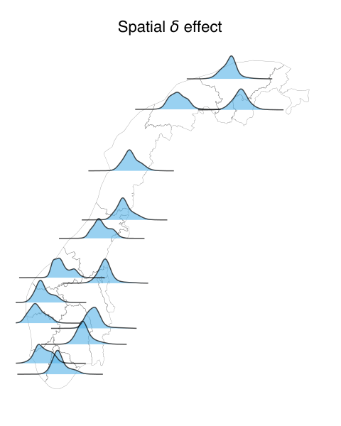
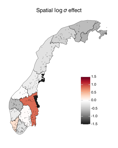
River-basin effects.

The most pronounced variation occurs between river-basin districts. The discrete spatial terms in the bottom row of Figure 12 show drastic regional differences in location and scale, but also in the shape of the standardized preview-density. Some districts have comparatively smooth unimodal previews, whereas others show marked skewness, shoulders, or multiple modes. Note that these are term-wise density previews: for each district, the shape predictor is evaluated with the remaining transformation terms held at zero; this means in particular that the preview densities here implicitly condition on lake-water. As Table 2 shows, the number of observations is uneven across districts and monitoring sites, so previews for sparsely observed regions should be interpreted with caution.

Table 2: Summary of observations and monitoring sites by river basin district for the Norwegian water-conductivity data.

River basin district		Counts		Observations per site
ID	Name	Observations	Sites	Median	Max.	Min.
NO1101	Moere and Romsdal	478	14	20.5	96	5
NO1102	Troendelag	$1{,}223$	39	19	234	1
NO1103	Nordland	603	29	6	213	1
NO1104	Troms	461	28	10	76	1
NO1105	Finnmark	300	11	7	219	4
NO1106	Norwegian - Finnish	689	24	20.5	157	7
NO2	Bothnian Sea	20	3	1	18	1
NO5	Skagerrak and Kattegat	106	8	9	27	3
NO5101	Glomma	$2{,}161$	43	20	801	1
NO5102	West-Bay	$2{,}398$	50	11.5	993	2
NO5103	Agder	$1{,}875$	58	20	268	2
NO5104	Rogaland	$1{,}985$	29	20	385	3
NO5105	Hordaland	470	18	12	136	2
NO5106	Sogn og Fjordane	656	16	24.5	155	3

The Glomma district provides a particularly clear example. Its preview shows a strong departure from unimodality, in addition to comparatively high location and scale effects. This pattern is plausibly related to the composition of the measurements in the district: about 38% of the Glomma observations were collected from the Alna River, mostly at a single intensively monitored site in Oslo. Thus, a regional density that pools several monitoring sites can become multimodal when those sites have persistently different conductivity levels. The PTM makes this heterogeneity visible as a structured shape effect.

6.1.4 Sensitivity to monitoring-site effects

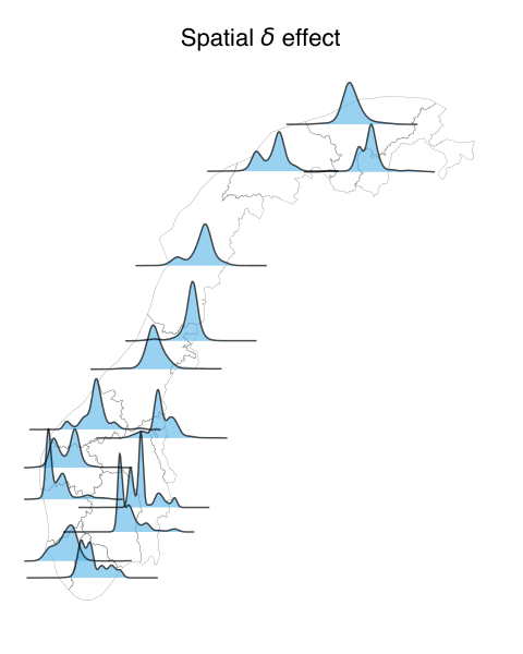
Adding site-specific random intercepts to the location and log-scale predictors absorbs much of the persistent between-site heterogeneity. In the resulting fit, shown in Figure D.4, the river-basin scale contrasts are strongly attenuated and the spatial shape previews become substantially more similar and predominantly unimodal, although some regional structure remains in location, scale, and shape. As in the focal fit, the day-of-year shape previews are essentially identical and not included in the figure. The water-body contrast is also strongly attenuated: both previews are broadly unimodal, with the river preview showing a lower, broader peak and lower density over the displayed upper range than the lake preview.

This sensitivity analysis illustrates a broader point about the interpretation of conditional-shape PTMs. A shape effect is conditional on the location and scale structure included elsewhere in the model. If persistent group-level shifts are omitted, their mixture can appear as skewness or multimodality and can be represented by the flexible transformation predictor. Adding the relevant grouping structure may then remove much of the apparent shape effect. This is not a contradiction: the pooled model describes heterogeneity across the sampled sites mainly through the broad discrete spatial effect, whereas the site-adjusted model can more closely represent the idiosyncrasies of particular sites. Importantly, the focal spatial effects should not be interpreted as intrinsic or causal properties of the river-basin districts. At the same time, their attenuation demonstrates how structured shape effects can serve as a diagnostic for unresolved heterogeneity and motivate a refined location–scale specification.

Predictive comparisons of the three distributional specifications, with and without monitoring-site effects, are summarized in Table 3. The conditional-shape PTM has the lowest PSIS-LOO and WAIC deviances both with and without monitoring-site effects; the fixed-shape PTM ranks second and the Gaussian model third. An expanded comparison including slightly varied model setups and corresponding transformed-residual Q–Q plots are provided in Table D.1 and Figure D.3, respectively. When including monitoring sites, we observed elevated numbers of Pareto- $k$ warnings, so the model ranking for the site-adjusted models should not be treated as conclusive; Section D.2 provides additional details.

Table 3: Predictive comparison of the models fitted in the two applications. Reported quantities are the PSIS-LOO and WAIC deviances, their standard errors (SE), and the corresponding effective numbers of parameters

p_{\mathrm{eff}}

PSIS-LOO
	Norwegian water conductivity
	Without site effects			With site effects			German temperature
Model	Deviance $\downarrow$	SE	$p_{\mathrm{eff}}$	Deviance $\downarrow$	SE	$p_{\mathrm{eff}}$	Deviance $\downarrow$	SE	$p_{\mathrm{eff}}$
CS-PTM	$18{,}515$	$210.6$	$393$	$-10{,}885$	$245.4$	$941$	$1{,}457{,}565$	$1{,}515.8$	$5{,}907$
FS-PTM	$24{,}009$	$222.9$	$109$	$-10{,}746$	$243.1$	$720$	$1{,}504{,}869$	$1{,}565.9$	$3{,}163$
Gaussian	$25{,}752$	$230.9$	$177$	$-9{,}472$	$273.1$	$1{,}098$	$1{,}511{,}783$	$1{,}572.8$	$4{,}833$
WAIC
CS-PTM	$18{,}481$	$209.4$	$376$	$-11{,}050$	$242.8$	$858$	$1{,}457{,}472$	$1{,}515.6$	$5{,}860$
FS-PTM	$24{,}007$	$222.9$	$108$	$-10{,}818$	$242.5$	$684$	$1{,}504{,}839$	$1{,}565.9$	$3{,}148$
Gaussian	$25{,}749$	$231.3$	$176$	$-9{,}826$	$266.2$	$921$	$1{,}511{,}737$	$1{,}572.7$	$4{,}810$

Note. The predictive criteria are reported on the deviance scale, defined as $-2$ times the corresponding expected log predictive density; smaller values indicate better predictive fit. Both criteria use draws from the fitted variational approximations. For both applications, these observation-level criteria use the working assumption of conditionally independent observations. Within each application and model category, the reported fit minimizes both criteria among the corresponding rows in Table D.1. CS-PTM and FS-PTM denote the conditional-shape and fixed-shape PTMs, respectively.

6.2 Daily air temperature in Germany

6.2.1 Data and scientific context

Our second application considers daily mean air temperature obtained from the quality-controlled historical daily station observations of the Climate Data Center of the German Weather Service (Deutscher Wetterdienst, DWD), version v24.3 (Deutscher Wetterdienst, 2024). The data were downloaded in 2026 and are distributed under the Creative Commons Attribution 4.0 International (CC BY 4.0) license. They cover the 20 complete calendar years from 2006 through 2025 and comprise $164$ monitoring stations distributed across Germany. After observations with missing temperature are removed, the analysis includes $1{,}182{,}514$ station-days. The station set contains all eligible stations above $900$ meters and a space-filling selection of stations at lower elevations. The response is daily mean temperature in degrees Celsius. Station elevations range from 0 to $1{,}486$ m, except for the outlying Zugspitze station at $2{,}956$ m. Ten stations lie above $900$ m. Their spatial distribution is shown in Figure 13.

Figure 13: Locations (left) and elevation distribution (right) of the 164 DWD monitoring stations included in the German daily-temperature application.

The design is an updated temperature adaptation of earlier structured additive distributional-regression applications to German precipitation (Umlauf et al., 2018; Kneib et al., 2019). Those analyses motivate the combination of seasonal, elevation, spatial, and space-season interaction effects used here, but the response, observation period, and interpretation differ. The application also provides a large-data example with more than one million observations that demonstrates the scalability of our approach. The model does not use recent weather observations or output from a weather-forecast model. It therefore describes how temperature distributions vary across place and time; it does not forecast the temperature on a specific future day.

6.2.2 Model specification

Let $\text{day}_{i}$ denote the day of the year³³ 3 Leap-day observations were retained when defining calendar day of year (1–366)., $\text{elev}_{i}$ denote station elevation, $(\text{lon}_{i},\text{lat}_{i})$ denote longitude and latitude, and $\text{year}_{i}$ denote the calendar year. Before fitting, we center and scale temperature using its empirical mean and standard deviation. Apart from adding a P-spline to capture the long-term effect of $\text{year}_{i}$ , we use the same broad predictor structure in the location, log-scale, and shape predictors as Umlauf et al. (2018) and Kneib et al. (2019),

\displaystyle\eta_{t,i}

\displaystyle=\gamma^{t}_{0}

\displaystyle+f^{t}_{1}(\text{day}_{i})

\displaystyle+f^{t}_{2}(\text{year}_{i})

\displaystyle+f^{t}_{3}(\text{elev}_{i})

\displaystyle+f^{t}_{4}(\text{lon}_{i})

\displaystyle+f^{t}_{5}(\text{lat}_{i})

\displaystyle+f^{t}_{6}(\text{day}_{i},\text{lon}_{i},\text{lat}_{i}),

\displaystyle\boldsymbol{\delta}(\boldsymbol{x}_{i})

\displaystyle=\boldsymbol{\delta}_{0}

\displaystyle+\boldsymbol{f}^{\delta}_{1}(\text{day}_{i})

\displaystyle+\boldsymbol{f}^{\delta}_{2}(\text{year}_{i})

\displaystyle+\boldsymbol{f}^{\delta}_{3}(\text{elev}_{i})

\displaystyle+\boldsymbol{f}^{\delta}_{4}(\text{lon}_{i})

\displaystyle+\boldsymbol{f}^{\delta}_{5}(\text{lat}_{i})

\displaystyle+\boldsymbol{f}^{\delta}_{6}(\text{day}_{i},\text{lon}_{i},\text{lat}_{i}),

for $t\in\{\mu,\sigma\}$ . The seasonal effects $f^{t}_{1}(\text{day}_{i})$ and $\boldsymbol{f}^{\delta}_{1}(\text{day}_{i})$ are cyclic P-splines, the other effects are univariate and bivariate P-splines, and $f^{t}_{6}$ and $\boldsymbol{f}^{\delta}_{6}$ are tensor-product terms that allow the seasonal pattern to vary over space and include the bivariate interactions. The conditional-shape PTM uses $D=10$ transformation parameters on the core interval $[-5,5]$ . We compare it with a fixed-shape PTM whose transformation has no covariate-dependent effects and with a Gaussian location–scale model, while retaining the same location and scale predictors. In the location and log-scale predictors, the day, year, and elevation smooths used basis dimension $k=20$ , the longitude and latitude main effects used $k=10$ , and each margin of the tensor-product effect used $k=10$ . The corresponding dimensions in the shape predictor were $k=10$ and $k=7$ , respectively. We calibrated the location and log-scale smoothing-variance priors as in Section 6.1. The within-covariate and between-transformation-dimension variances in the shape predictor independently followed $\operatorname{Weibull}(1/2,0.05)$ priors. The variational approximation used separate dense blocks for moderate-dimensional main-effect terms (including the main-effect terms in the shape predictor) and diagonal blocks for the tensor-product interactions.

Additional details on the optimization settings are included in Section D.1.

6.2.3 Results

On a MacBook Pro with a 10-core Apple M1 Pro processor and 32 GB of memory, the staged PTM fit took approximately 74 minutes.

Predictive performance and location–scale effects.

The predictive criteria in Table 3 favor the PTM. An expanded comparison in Table D.1 shows that other conditional-shape PTM variants with slightly varied setups likewise outperform the fixed-shape PTM and Gaussian models, with the focal $D=10$ , $[-5,5]$ specification attaining the best performance in both criteria. Figure D.3 provides transformed-residual Q–Q plots. Figure 14 summarizes the results. The location effects show the expected seasonal, spatial, and elevation-related temperature variation, while the scale effects reveal distinct patterns in conditional dispersion. The seasonal contribution reaches its minimum in late January and its maximum in late July to early August. Across the nine focal cities, the seasonal posterior mean effects excluding spatial main contributions range from $-9.99$ to $-8.18\,{}^{\circ}\mathrm{C}$ at the winter minima and from $7.98$ to $9.66\,{}^{\circ}\mathrm{C}$ at the summer maxima. The cities share a broadly similar seasonal location pattern, with modest spatial variation mainly in the amplitude of the annual cycle. The seasonal log-scale contribution is largest in winter, corresponding to multiplicative scale factors of $1.24$ – $1.34$ , and smallest in late September, with factors of $0.76$ – $0.84$ . These factors exponentiate the posterior mean of the seasonal main effect plus the space-season interactions on the log-scale predictor; they are partial scale contributions, not complete conditional standard deviations.

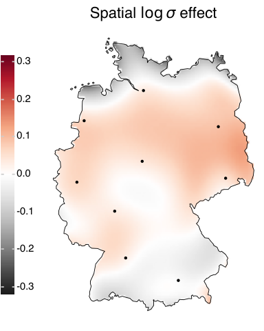
The spatial location effect shows a broad north-south gradient, with lower temperature over much of northern and northeastern Germany and higher temperature in the south. In contrast, the spatial log-scale effect is positive across a broad central-to-eastern region and negative along the northern coast and in parts of southern Germany. The fitted year effect on location oscillates but trends upward as successive low and high points generally increase. This pattern is consistent with general warming, but it should be noted that this is a descriptive conditional result for the selected station network, not a causal or nationally representative trend estimate. The year effect on log scale is also non-monotone, and it is smaller than the seasonal scale variation.

The elevation effect on location decreases almost linearly by about $15$ – $16\,{}^{\circ}\mathrm{C}$ between sea level and $3{,}000$ m, equivalent on average to roughly $5\,{}^{\circ}\mathrm{C}$ per $1{,}000$ m. The log-scale effect increases over the well-supported elevation range. There are no stations between $1{,}486$ and $2{,}956$ m, and the posterior intervals for the two elevation effects widen accordingly. The broad interpolation across the gap is generally plausible, but its shape is not directly supported by observations. The near-overlap of the elevation density previews indicates that the corresponding shape effect is strongly regularized.

Figure 15: Seasonal distribution summaries for the PTM at the nine locations in the German daily-temperature application. The top row shows diagnostic posterior mean standardized quantiles at

p\in\{0.01,0.5,0.99\}

. Colored curves combine the shape intercept with the seasonal, spatial main, and space-season interaction terms, while black curves retain only the shape intercept and seasonal main effect; year and elevation shape effects are omitted. Gray dashed lines mark the corresponding standard Gaussian quantiles. The middle row shows complete conditional quantiles in degrees Celsius during 2015 at the city-specific elevations. The lower panels show the corresponding complete conditional densities on two representative days. Colored rug marks on the horizontal axes indicate the location-specific

p\in\{0.01,0.5,0.99\}

quantiles. Credible interval ribbons are omitted to avoid clutter. Corresponding summaries for the fixed-shape PTM and Gaussian location–scale model are shown in Figure D.1 and Figure D.2, respectively.

Standardized shape effects.

The seasonal density previews in the right column of Figure 14 suggest a reversal in asymmetry: winter previews extend farther toward the lower end of the displayed range, whereas summer previews extend farther toward the upper end of the displayed range.

The top row of Figure 15 probes this asymmetry at the displayed $p=0.01$ and $p=0.99$ quantiles more directly. During much of summer, the fitted $p=0.99$ quantile exceeds the corresponding standard Gaussian quantile at most focal locations, placing the displayed upper quantile farther from zero, while the fitted $p=0.01$ quantile is less negative at all nine locations, placing the displayed lower quantile closer to zero. Munich is the clearest exception for the upper quantile: its summer $p=0.99$ curve remains near or below the Gaussian reference. In winter and early spring, the fitted $p=0.99$ quantiles are generally less extreme than the Gaussian reference, whereas the fitted $p=0.01$ quantiles are more negative, so the displayed upper quantile lies closer to zero and the lower quantile lies farther from zero. Because all displayed distributions have mean zero and variance one, these movements describe pure shape changes, isolated from location and scale.

The seasonal shape pattern also shows substantial spatial variation, most prominently in the extreme quantiles. During the plotted summer window, Meppen’s $p=0.99$ quantile reaches $2.84$ , whereas Munich’s peaks at $2.24$ ; differences among locations are smaller at $p=0.5$ . The changing gaps between the colored curves and the black seasonal-main-effect curve indicate that spatial shape effects interact with the seasonal pattern rather than acting as fixed offsets.

However, note that the density previews in Figure 14 and the derived quantile curves in Figure 15 should not be confused with full conditional densities or quantiles of full conditional distributions. They are instead probes that allow us to inspect how seasonal and spatial shape terms modify the reference distribution in isolation, giving us insight into how the model arrives at its predictions.

Complete conditional distributions.

Panels b and c of Figure 15 show how the fitted location, scale, and shape effects combine into complete conditional quantiles and densities on the temperature scale, where the seasonal location effect is dominant. Figure D.1 and Figure D.2 provide companion displays for the fixed-shape PTM and Gaussian location–scale model. The colored rug marks in the lower panels show the posterior mean complete conditional quantiles at $p\in\{0.01,0.5,0.99\}$ ; Table D.2 reports the exact values.

The conditional-shape PTM’s added shape flexibility can alter quantile predictions even when the fitted centers are nearly unchanged. For Meppen on July 15, the $(p=0.01,0.5,0.99)$ quantiles are $(12.03,17.95,27.01)\,{}^{\circ}\mathrm{C}$ under the conditional-shape model, $(11.00,18.29,25.66)\,{}^{\circ}\mathrm{C}$ under the fixed-shape model, and $(10.69,18.14,25.59)\,{}^{\circ}\mathrm{C}$ under the Gaussian model. The conditional-shape model and Gaussian medians differ by only $0.19\,{}^{\circ}\mathrm{C}$ , but the distances from the conditional-shape model median to its lower and upper quantiles are $5.92$ and $9.06\,{}^{\circ}\mathrm{C}$ , respectively, compared with $7.45\,{}^{\circ}\mathrm{C}$ in both directions under the Gaussian model. The farther extension into the displayed upper range of Meppen’s summer density in panel c makes this unequal quantile spacing visible.

Munich on January 15 shows the reverse pattern: its $p=0.01$ curve reaches particularly low winter values in panel b, and its blue density in panel c extends farther into the displayed lower range. The conditional-shape model $p=0.01$ , $0.5$ , and $0.99$ quantiles are $-13.30$ , $0.09$ , and $9.22\,{}^{\circ}\mathrm{C}$ , respectively. The corresponding values are $-9.54$ , $0.05$ , and $9.73\,{}^{\circ}\mathrm{C}$ for the fixed-shape model and $-9.91$ , $-0.08$ , and $9.75\,{}^{\circ}\mathrm{C}$ for the Gaussian model. The fitted medians again differ little, while the conditional-shape model has a substantially lower $p=0.01$ quantile and a slightly lower $p=0.99$ quantile than both comparison models. Across all nine locations, its winter $p=0.01$ quantiles are $1.67$ – $3.75\,{}^{\circ}\mathrm{C}$ below those of the fixed-shape model and $1.42$ – $3.39\,{}^{\circ}\mathrm{C}$ below those of the Gaussian model.

Together, the figures and predictive comparison show how the PTM preserves a familiar location–scale interpretation while adding controlled shape flexibility where the data support it.

7 Discussion

Conditional-shape PTMs extend the PTM family from structured additive location–scale regression to settings in which covariates may also affect distributional shape. The model is constructed to include the conditional mean $\mu(\boldsymbol{x})$ and standard deviation $\sigma(\boldsymbol{x})$ of the response, while the transformation predictor $\boldsymbol{\delta}(\boldsymbol{x})$ controls the standardized shape of the response’s conditional distribution. Its vector-valued structured additive terms allow scientifically motivated covariate effects, and their penalties regularize departures from a reference-family (usually Gaussian) location–scale model. The construction thus combines a coherent conditional distribution with an explicit separation of location, scale, and shape.

The empirical results support this contribution at three distinct levels. In the controlled setting of simulation Scenario A, the PTM recovers the response-level effects and the covariate-dependent transition from skewness to bimodality; in the Gaussian subscenario, its predictive performance is nearly identical to that of the simpler nested models, indicating effective regularization of unnecessary transformation flexibility. Under the deliberate misspecification of Scenario B, the PTM improves with sample size and performs approximately as well as a Dirichlet process mixture model in terms of test-set Kullback–Leibler divergence and CDF deviation. The two applications illustrate a complementary benefit. The PTM retains seasonal, spatial, temporal, or group-specific shape variation while strongly regularizing other shape effects, and it improves PSIS-LOO and WAIC relative to both simpler comparison models.

Methodologically, conditional-shape PTMs occupy a middle ground between parsimonious location–scale regression and less structured conditional-density methods. They are most useful when a flexible estimate of a complete conditional distribution is required, the first two conditional moments should retain exact response-scale interpretations, and substantive knowledge suggests which covariates may change shape. A Gaussian location–scale model is preferable when its residual shape is adequate, and a fixed-shape PTM is more economical when a single non-Gaussian standardized distribution suffices. A well-supported parametric distributional model may be more parsimonious, while quantile regression is natural when only selected quantiles are the estimands and mixture-based or other flexible density regression may be preferable when unrestricted predictive density estimation is primary. The distinctive role of the conditional-shape PTM is therefore structured control over where distributional flexibility enters, not universal dominance over these alternatives.

The construction also suggests a practical fitting and interpretation strategy. Scientifically important grouping, location, and scale effects should be specified before residual skewness or multimodality is attributed to shape. The reference distribution and spline-core boundaries $a$ and $b$ should reflect defensible tail assumptions, because changing the core support can extend finite-range flexibility but cannot change the asymptotic tail class. Shape effects can be probed through contrasts in standardized preview densities or standardized conditional quantiles. This decomposability is an interpretive advantage of the conditional-shape PTM, but the resulting partial summaries should not be mistaken for response-scale predictions or for densities marginalized over the remaining covariates. Predictive interpretation requires the complete shape, location, and scale predictors. Fitted models can be checked using transformed-residual Q–Q plots.

Four principal limitations should be noted. First, the blocked Gaussian variational approximation omits cross-block posterior dependence and non-Gaussian posterior features, and no exact-posterior PTM benchmark is available. This family is comparatively rudimentary relative to recent approaches for additive and distributional regression (Kleinemeier and Klein, 2023; Lichter et al., 2024; Callegher et al., 2026). In additive-model comparisons, retaining dependence among coefficient blocks was crucial for calibrated credible intervals even when point estimates were similar (Lichter et al., 2024). The undercoverage in Scenario B cannot be attributed to this approximation alone because every model is misspecified to some degree there, but it shows that good predictive point summaries do not guarantee calibrated uncertainty. Second, shape effects are conditional on the full model specification: omitted grouping structures or interactions can be absorbed as apparent shape effects, as demonstrated by the Norwegian sensitivity analysis and the unmodeled interaction in Scenario B. In practice, users should therefore check whether shape effects point to influences of hidden covariates. Third, the identity-tailed transformation inherits the asymptotic tail class of the reference distribution. It can flexibly describe distributions over the spline core, but it cannot learn a fundamentally different limiting tail behavior. Finally, the hyperprior for the between-parameter smoothing variance $\psi^{2}$ was chosen pragmatically based on an intercept-only prior check. Its implied regularization need not be comparable across shape terms with different bases, penalties, or covariate domains. These limitations motivate three focused extensions: richer structured posterior approximations, shape-effect priors calibrated on an interpretable distributional deviation scale, and transformations that permit more flexible tail adaptation without sacrificing the mean-standard-deviation separation.

Conditional-shape PTMs provide a principled and practical extension of interpretable location–scale regression: they permit scientifically targeted changes in distributional shape within one coherent conditional distribution and regularize toward a simpler reference model when that flexibility is unsupported.

Data and code availability

The data and code supporting this study are currently available upon request. They will be made publicly available upon submission to a journal or in a forthcoming update.

Acknowledgments

The authors used OpenAI Codex with the GPT-5.6 Sol model for coding and writing assistance. All generated outputs were critically reviewed and revised by the authors. The authors maintain sole responsibility for the software, analyses, interpretations, and final manuscript.

Conflict of interest

The authors declare no conflicts of interest.

Funding

We are grateful to the German Research Foundation (DFG) for financial support through grant 443179956.

References

Bach and Klein (2025) P. Bach and N. Klein Anisotropic multidimensional smoothing using Bayesian tensor product P-splines. 35 (2). External Links: Document Cited by: Appendix A.
Baumann et al. (2021) P. F. M. Baumann, T. Hothorn, and D. Rügamer Deep conditional transformation models. In Machine Learning and Knowledge Discovery in Databases. Research Track, N. Oliver, F. Pérez-Cruz, S. Kramer, J. Read, and J. A. Lozano (Eds.), Lecture Notes in Computer Science, Vol. 12977, pp. 3–18. External Links: Document Cited by: §1, §1, §3.
Bondell et al. (2010) H. D. Bondell, B. J. Reich, and H. Wang Noncrossing quantile regression curve estimation. 97 (4), pp. 825–838. External Links: Document Cited by: §1.
Brachem et al. (2026a) Liesel-GAM: generalized additive models in Liesel External Links: Link Cited by: §1, §3, §4.4.
Brachem et al. (2026b) J. Brachem, P. F. V. Wiemann, and M. KatzfussData-efficient generative modeling of non-Gaussian global climate fields via scalable composite transformations(Website) External Links: Document Cited by: §2.1, §2.1.
Brachem et al. (2026c) J. Brachem, P. F. V. Wiemann, and T. Kneib Bayesian penalized transformation models: structured additive location-scale regression for arbitrary conditional distributions. pp. 1–16. External Links: Document Cited by: §1, §2.1, §3, §4, §5.1.
Brachem et al. (2026d) Liesel-PTM: penalized transformation models in Liesel External Links: Link Cited by: §1, §2.1, §4.4.
Callegher et al. (2026) G. Callegher, T. Kneib, J. Söding, and P. WiemannStochastic variational inference for structured additive distributional regression(Website) External Links: 2412.10038v3, Document Cited by: §1, §4.2, §4, §7.
Carlan et al. (2024) M. Carlan, T. Kneib, and N. Klein Bayesian conditional transformation models. 119 (546), pp. 1360–1373. External Links: Document Cited by: §1.
Deutscher Wetterdienst (2024) Deutscher Wetterdienst Daily station observations (temperature, pressure, precipitation, sunshine duration, etc.) for Germany. DWD Climate Data Center (CDC). Note: Dataset ID: urn:wmo:md:de-dwd-cdc:obsgermany-climate-daily-kl; licensed under CC BY 4.0 External Links: Link Cited by: §6.2.1.
European Environment Agency (2025) European Environment Agency Waterbase—water quality ICM, 2024. European Environment Agency. External Links: Link Cited by: §6.1.1.
Fahrmeir et al. (2013) L. Fahrmeir, T. Kneib, S. Lang, and B. Marx Regression: models, methods and applications. Springer. External Links: Document Cited by: §A.2.
Fasiolo et al. (2021) M. Fasiolo, S. N. Wood, M. Zaffran, R. Nedellec, and Y. Goude Fast calibrated additive quantile regression. 116 (535), pp. 1402–1412. External Links: Document Cited by: §1.
Gelman (2006) A. Gelman Prior distributions for variance parameters in hierarchical models (comment on article by Browne and Draper). 1 (3), pp. 515–533. External Links: Document Cited by: Appendix A.
Greven and Scheipl (2017) S. Greven and F. Scheipl A general framework for functional regression modelling. 17 (1–2), pp. 1–35. External Links: Document Cited by: §1, §3.
Hoffman et al. (2013) M. D. Hoffman, D. M. Blei, C. Wang, and J. Paisley Stochastic variational inference. 14 (40), pp. 1303–1347. External Links: Link Cited by: §4.1.
Hothorn et al. (2014) T. Hothorn, T. Kneib, and P. Bühlmann Conditional transformation models. 76 (1), pp. 3–27. External Links: Document Cited by: §1.
Hothorn et al. (2018) T. Hothorn, L. Möst, and P. Bühlmann Most likely transformations. 45 (1), pp. 110–134. External Links: Document Cited by: §1.
Kaushal et al. (2021) S. S. Kaushal, G. E. Likens, M. L. Pace, J. E. Reimer, C. M. Maas, J. G. Galella, R. M. Utz, S. Duan, J. R. Kryger, A. M. Yaculak, W. L. Boger, N. W. Bailey, S. Haq, K. L. Wood, B. M. Wessel, C. E. Park, D. C. Collison, B. Y. I. Aisin, T. M. Gedeon, S. K. Chaudhary, J. Widmer, C. R. Blackwood, C. M. Bolster, M. L. Devilbiss, D. L. Garrison, S. Halevi, G. Q. Kese, E. K. Quach, C. M. P. Rogelio, M. L. Tan, H. J. S. Wald, and S. A. Woglo Freshwater salinization syndrome: from emerging global problem to managing risks. 154 (2), pp. 255–292. External Links: Document Cited by: §6.1.1.
Klein et al. (2015a) N. Klein, T. Kneib, S. Klasen, and S. Lang Bayesian structured additive distributional regression for multivariate responses. 64 (4), pp. 569–591. External Links: Document Cited by: §A.2.
Klein et al. (2015b) N. Klein, T. Kneib, S. Lang, and A. Sohn Bayesian structured additive distributional regression with an application to regional income inequality in Germany. 9 (2), pp. 1024–1052. External Links: Document Cited by: §1.
Klein and Kneib (2016) N. Klein and T. Kneib Scale-dependent priors for variance parameters in structured additive distributional regression. 11 (4), pp. 1071–1106. External Links: Document Cited by: Appendix A, §3, §6.1.2.
Kleinemeier and Klein (2023) J. Kleinemeier and N. KleinScalable estimation for structured additive distributional regression through variational inference(Website) External Links: Document Cited by: §1, §4.2, §4, §7.
Kneib et al. (2019) T. Kneib, N. Klein, S. Lang, and N. Umlauf Modular regression—a Lego system for building structured additive distributional regression models with tensor product interactions. 28 (1), pp. 1–39. External Links: Document Cited by: Appendix A, Appendix A, §1, §6.2.1, §6.2.2.
Kowal and Wu (2025) D. R. Kowal and B. Wu Monte Carlo inference for semiparametric Bayesian regression. 120 (550), pp. 1063–1076. External Links: Document Cited by: §1.
Kucukelbir et al. (2017) A. Kucukelbir, D. Tran, R. Ranganath, A. Gelman, and D. M. Blei Automatic differentiation variational inference. 18 (14), pp. 1–45. External Links: Link Cited by: §1, §4.1.
Lichter et al. (2024) J. Lichter, P. F. V. Wiemann, and T. Kneib Variational inference: uncertainty quantification in additive models. 108 (2), pp. 279–331. External Links: Document Cited by: §1, §4.2, §4, §7.
Maier et al. (2025) E. Maier, A. Fottner, S. Greven, and A. StöckerAdditive density regression(Website) External Links: Document Cited by: §1.
Riebl et al. (2026) H. Riebl, J. Brachem, T. Kneib, G. Callegher, and P. F. V. WiemannLiesel: a Python framework for graph-based Bayesian modeling and customizable MCMC with support for generalized additive models(Website) External Links: Document Cited by: §1, §4.4.
Rigby and Stasinopoulos (2005) R. A. Rigby and D. M. Stasinopoulos Generalized additive models for location, scale and shape. 54 (3), pp. 507–554. External Links: Document Cited by: §1.
Rodríguez-Álvarez et al. (2025) M. X. Rodríguez-Álvarez, V. Inácio, and N. Klein Density regression via Dirichlet process mixtures of normal structured additive regression models. 35 (2). External Links: Document Cited by: §1, §5.1.
Rue and Held (2005) H. Rue and L. Held Gaussian Markov random fields: theory and applications. Monographs on Statistics and Applied Probability, Chapman & Hall/CRC. External Links: Document Cited by: 3rd item.
Scheipl et al. (2015) F. Scheipl, A. Staicu, and S. Greven Functional additive mixed models. 24 (2), pp. 477–501. External Links: Document Cited by: §1, §3.
Sick et al. (2021) B. Sick, T. Hothorn, and O. Dürr Deep transformation models: tackling complex regression problems with neural network based transformation models. In 2020 25th International Conference on Pattern Recognition (ICPR), pp. 2476–2481. External Links: Document Cited by: §1.
Siegfried et al. (2023) S. Siegfried, L. Kook, and T. Hothorn Distribution-free location-scale regression. 77 (4), pp. 345–356. External Links: Document Cited by: §1.
Simpson et al. (2017) D. Simpson, H. Rue, A. Riebler, T. G. Martins, and S. H. Sørbye Penalising model component complexity: a principled, practical approach to constructing priors. 32 (1), pp. 1–28. External Links: Document Cited by: Appendix A.
Titsias and Lázaro-Gredilla (2014) M. K. Titsias and M. Lázaro-Gredilla Doubly stochastic variational Bayes for non-conjugate inference. In Proceedings of the 31st International Conference on Machine Learning, Proceedings of Machine Learning Research, Vol. 32, pp. 1971–1979. External Links: Link Cited by: §4.1.
Umlauf et al. (2018) N. Umlauf, N. Klein, and A. Zeileis BAMLSS: Bayesian additive models for location, scale, and shape (and beyond). 27 (3), pp. 612–627. External Links: Document Cited by: §1, §6.2.1, §6.2.2.
Vehtari et al. (2017) A. Vehtari, A. Gelman, and J. Gabry Practical Bayesian model evaluation using leave-one-out cross-validation and WAIC. 27 (5), pp. 1413–1432. External Links: Document Cited by: §5.1.
Waldmann et al. (2013) E. Waldmann, T. Kneib, Y. R. Yue, S. Lang, and C. Flexeder Bayesian semiparametric additive quantile regression. 13 (3), pp. 223–252. External Links: Document Cited by: §1.
Wiemann et al. (2026) Liesel: a probabilistic programming framework External Links: Link Cited by: §4.4.

Appendix A Details for multivariate structured additive predictors

This appendix collects the derivations, computational details, and examples supporting the compact formulation in Section 3.

Expanding the predictor into its $D$ elements and the basis vector into its $K$ terms yields

\displaystyle\begin{bmatrix}\eta_{1}\\ \vdots\\ \eta_{D}\\ \end{bmatrix}\hskip 8.50012pt=\hskip 8.50012pt\begin{bmatrix}f_{1,1}(\boldsymbol{x})\\ \vdots\\ f_{D,1}(\boldsymbol{x})\\ \end{bmatrix}+\cdots+\begin{bmatrix}f_{1,K}(\boldsymbol{x})\\ \vdots\\ f_{D,K}(\boldsymbol{x})\\ \end{bmatrix}\hskip 8.50012pt=\hskip 8.50012pt\begin{bmatrix}\boldsymbol{\gamma}^{\top}_{1,1}&\cdots&\boldsymbol{\gamma}^{\top}_{1,K}\\ \vdots&\ddots&\vdots\\ \boldsymbol{\gamma}^{\top}_{D,1}&\cdots&\boldsymbol{\gamma}^{\top}_{D,K}\\ \end{bmatrix}\begin{bmatrix}\mathbf{b}_{1}(\boldsymbol{x})\\ \vdots\\ \mathbf{b}_{K}(\boldsymbol{x})\\ \end{bmatrix}.

(16)

Between-dimension regularization.

Between-dimension regularization is governed by the matrix $\mathbf{P}^{(d)}(\psi^{2}_{k})=\psi^{-2}_{k}\mathbf{K}_{k}^{(d)}$ , where $\mathbf{K}_{k}^{(d)}$ is a constant, potentially rank-deficient positive-semidefinite penalty matrix that defines the correlation structure. The variance parameter $\psi^{2}_{k}$ acts as an inverse smoothing parameter, so smaller values imply stronger between-dimension regularization for term $k$ . The structural penalty matrix $\mathbf{K}_{k}^{(d)}$ is chosen manually to define an appropriate correlation pattern.

Within-dimension regularization.

In the most general case, the matrix $\mathbf{P}^{(x)}_{k}(\boldsymbol{\tau}^{2}_{k})$ is an anisotropic tensor-product precision matrix that defines the within-dimension regularization in the covariate directions. The variance parameters in $\boldsymbol{\tau}^{2}_{k}=[\tau^{2}_{k,1},\dots,\tau^{2}_{k,M_{k}}]^{\top}$ control the strength of regularization. For an $M_{k}$ -dimensional tensor product, it is given by the sum

\mathbf{P}^{(x)}_{k}(\boldsymbol{\tau}^{2}_{k})=\tau^{-2}_{k,1}\widetilde{\mathbf{K}}^{(x)}_{k,1}+\cdots+\tau^{-2}_{k,M_{k}}\widetilde{\mathbf{K}}^{(x)}_{k,M_{k}}

with the individual $\widetilde{\mathbf{K}}^{(x)}_{k,m}$ for $m=1,\dots,M_{k}$ given by

\widetilde{\mathbf{K}}^{(x)}_{k,m}=\mathbf{I}_{L_{k,1}}\otimes\cdots\otimes\mathbf{I}_{L_{k,m-1}}\otimes\mathbf{K}^{(x)}_{k,m}\otimes\mathbf{I}_{L_{k,m+1}}\otimes\cdots\otimes\mathbf{I}_{L_{k,M_{k}}},

such that $\mathbf{K}^{(x)}_{k,m}$ is the constant, potentially rank-deficient positive-semidefinite penalty matrix defining the correlation structure in the $m$ th covariate direction of term $k$ .

Hyperpriors for variance parameters.

Hyperprior choices for variance parameters can be based on the considerations for hierarchical models outlined by Gelman (2006) and the concept of penalized model complexity developed by Simpson et al. (2017) and adapted to structured additive models by Klein and Kneib (2016). This leads to $\operatorname{Weibull}(1/2,\theta)$ priors for smoothing variances $\tau^{2}$ and $\psi^{2}$ , which favor the base models reached as the variance parameters approach zero while retaining a right tail that permits larger scales. The parameter $\theta$ denotes the scale of the hyperprior and can be chosen using an appropriate scaling criterion; see Klein and Kneib (2016). Other common hyperprior choices include inverse-gamma, half-normal, and half-Cauchy distributions; see Gelman (2006) and Klein and Kneib (2016) for discussions of their merits.

Joint prior.

The joint prior for all parameters in a multivariate structured additive predictor factors into the priors for the parameters and hyperparameters of the terms:

	$\displaystyle p(\boldsymbol{\Gamma},\boldsymbol{\tau}^{2},\boldsymbol{\psi}^{2})$	$\displaystyle=p(\boldsymbol{\Gamma}\mid\boldsymbol{\tau}^{2},\boldsymbol{\psi}^{2})\,p(\boldsymbol{\tau}^{2})\,p(\boldsymbol{\psi}^{2})$		(17)
		$\displaystyle=\left[\prod_{k=1}^{K}p(\boldsymbol{\gamma}_{k}\|\boldsymbol{\tau}^{2}_{k},\psi^{2}_{k})\right]\times\left[\prod_{k=1}^{K}\prod_{m=1}^{M_{k}}p(\tau^{2}_{k,m})\right]\times\left[\prod_{k=1}^{K}p(\psi^{2}_{k})\right],$		(18)

where $\boldsymbol{\tau}^{2}=[\boldsymbol{\tau}^{2\top}_{1},\dots,\boldsymbol{\tau}^{2\top}_{K}]^{\top}$ and $\boldsymbol{\psi}^{2}=[\psi^{2}_{1},\dots,\psi^{2}_{K}]^{\top}$ .

Computational efficiency.

Direct evaluation of the prior density (11) is computationally expensive because it requires computing $\operatorname{pdet}(\mathbf{P}_{k})$ . However, the structure of $\mathbf{P}_{k}$ allows between-dimension regularization to be treated as an additional direction in an anisotropic tensor-product smooth. The log-pseudo-determinant can therefore be computed efficiently from eigendecompositions of the constant, relatively low-dimensional penalty matrices $\mathbf{K}^{(x)}_{k,1},\dots,\mathbf{K}^{(x)}_{k,M_{k}}$ and $\mathbf{K}^{(d)}_{k}$ , as described in Theorem 3.1 and Corollary 3.2 of Bach and Klein (2025). For a given model, these eigendecompositions need to be computed only once, greatly reducing the cost of subsequent prior-density evaluations.

Linear constraints.

Linear constraints can be applied to the within-dimension and cross-dimension directions of a term. These two cases correspond to the two axes of the coefficient matrix $\boldsymbol{\Gamma}_{k}$ . We apply the reparameterization approach described by Kneib et al. (2019). We first consider a within-dimension constraint with full-row-rank matrix $\mathbf{A}_{k}^{(x)}\in\mathbb{R}^{r_{k}\times L_{k}}$ . Requiring the constraint to hold in each of the $D$ predictor dimensions gives $\boldsymbol{\Gamma}_{k}\mathbf{A}_{k}^{(x)\top}=\mathbf{0}_{D\times r_{k}}$ . Now let $\mathbf{Q}_{k}^{(x)}\in\mathbb{R}^{L_{k}\times(L_{k}-r_{k})}$ have orthonormal columns spanning the null space of $\mathbf{A}_{k}^{(x)}$ . The constraint can then be enforced by writing the term as $\boldsymbol{f}_{k}(\boldsymbol{x})=\overline{\boldsymbol{\Gamma}}_{k}\overline{\mathbf{b}}_{k}(\boldsymbol{x})$ , where $\overline{\mathbf{b}}_{k}(\boldsymbol{x})=\mathbf{Q}_{k}^{(x)\top}\mathbf{b}_{k}(\boldsymbol{x})$ is a reparameterized basis and $\overline{\boldsymbol{\Gamma}}_{k}\in\mathbb{R}^{D\times(L_{k}-r_{k})}$ is a reparameterized coefficient matrix whose prior uses reparameterized within-dimension penalty matrices $\mathbf{Q}_{k}^{(x)\top}\widetilde{\mathbf{K}}_{k,m}^{(x)}\mathbf{Q}_{k}^{(x)}$ . In the following, we suppress the bars: $\mathbf{b}_{k}(\boldsymbol{x})$ and $L_{k}$ denote the reparameterized covariate basis and its dimension, while $\boldsymbol{\Gamma}_{k}$ denotes the corresponding coefficient matrix. The same convention applies to $\widetilde{\mathbf{K}}_{k,m}^{(x)}$ .

Now let $\mathbf{A}^{(d)}\boldsymbol{\Gamma}_{k}=\mathbf{0}_{q\times L_{k}}$ be a constraint in the cross-dimensional direction with constraint matrix $\mathbf{A}^{(d)}\in\mathbb{R}^{q\times D}$ , and let $\mathbf{Q}^{(d)}\in\mathbb{R}^{D\times(D-q)}$ have orthonormal columns spanning the null space of $\mathbf{A}^{(d)}$ . Then the constraint can be applied by writing $\boldsymbol{\Gamma}_{k}=\mathbf{Q}^{(d)}\widetilde{\boldsymbol{\Gamma}}_{k}$ , where $\widetilde{\boldsymbol{\Gamma}}_{k}\in\mathbb{R}^{(D-q)\times L_{k}}$ is a reparameterized coefficient matrix whose prior uses the reparameterized cross-dimension penalty matrix $\mathbf{Q}^{(d)\top}\mathbf{K}_{k}^{(d)}\mathbf{Q}^{(d)}$ . Since a cross-dimensional constraint typically applies to all terms in a predictor, the reconstruction back into $D$ dimensions can be factored out and applied once after summing all reduced terms via $\boldsymbol{\eta}=\boldsymbol{\Gamma}\mathbf{b}(\boldsymbol{x})=\mathbf{Q}^{(d)}\{[\widetilde{\boldsymbol{\Gamma}}_{1},\dots,\widetilde{\boldsymbol{\Gamma}}_{K}]\mathbf{b}(\boldsymbol{x})\}$ .

The reparameterization matrices can be obtained from an eigendecomposition of $\mathbf{A}^{\top}\mathbf{A}$ : the eigenvectors associated with zero eigenvalues form an orthonormal basis $\mathbf{Q}$ of the null space of $\mathbf{A}$ ; see Section 2.3.2 of Kneib et al. (2019) for details.

A.1 Examples of term structures

The general framework outlined above simplifies considerably for many concrete models. We include four common examples of specific term definitions below.

Intercept in multiple dimensions.

An intercept $\boldsymbol{f}_{k}(\boldsymbol{x})=\boldsymbol{\gamma}_{k}$ is characterized by a scalar, constant basis $\mathbf{b}_{k}(\boldsymbol{x})~=~1$ , implying $M_{k}=1$ and a single zero-penalty in the covariate direction, $\mathbf{K}_{k}^{(x)}=0$ . In this case, the prior precision matrix simplifies to

\mathbf{P}_{k}=\mathbf{P}_{k}(\psi^{2}_{k})=\psi_{k}^{-2}\mathbf{K}^{(d)}_{k},

and the dimension of $\boldsymbol{\gamma}_{k}$ reduces to $(D\times 1)$ .

Univariate term in multiple dimensions.

A univariate term $\boldsymbol{f}_{k}(\boldsymbol{x})=\boldsymbol{f}_{k}(x_{im})$ is characterized by a basis function that is constant in all except one of the covariates in $\boldsymbol{x}=[x_{1},\dots,x_{M}]^{\top}$ , so the basis becomes $\mathbf{b}_{k}(\boldsymbol{x})~=~\mathbf{b}_{k}(x_{m})$ for some $m\in\{1,\dots,M\}$ , implying $M_{k}=1$ . The covariate-related component of the prior precision matrix then simplifies to the $(L_{k,m}\times L_{k,m})$ matrix

\mathbf{P}_{k}^{(x)}(\boldsymbol{\tau}^{2}_{k})=\mathbf{P}_{k}^{(x)}(\tau^{2}_{k,m})=\tau^{-2}_{k,m}\mathbf{K}^{(x)}_{k,m}.

Consequently, the full prior precision matrix is

\mathbf{P}_{k}=\mathbf{P}_{k}(\tau^{2}_{k,m},\psi^{2}_{k})=\frac{1}{\tau^{2}_{k,m}}\left(\mathbf{K}^{(x)}_{k,m}\otimes\mathbf{I}_{D}\right)+\frac{1}{\psi^{2}_{k}}\left(\mathbf{I}_{L_{k,m}}\otimes\mathbf{K}^{(d)}_{k}\right)

and $\boldsymbol{\gamma}_{k}$ has dimension $(DL_{k,m}\times 1)$ .

Bivariate tensor product term in multiple dimensions.

A bivariate tensor product term $\boldsymbol{f}_{k}(\boldsymbol{x})=\boldsymbol{f}_{k}(x_{m},x_{m^{\prime}})$ for $m,m^{\prime}\in\{1,\dots,M\}$ and $m\neq m^{\prime}$ is characterized by a basis function that is a tensor product of two marginal univariate bases of potentially different dimensions,

\underset{\scriptscriptstyle L_{k,m}L_{k,m^{\prime}}\times 1}{\mathbf{b}_{k}(\boldsymbol{x})}=\mathbf{b}_{k}(x_{m},x_{m^{\prime}})=\underset{\scriptscriptstyle L_{k,m}\times 1}{\mathbf{b}_{k,m}(x_{m})}\otimes\underset{\scriptscriptstyle L_{k,m^{\prime}}\times 1}{\mathbf{b}_{k,m^{\prime}}(x_{m^{\prime}})},

implying $M_{k}=2$ . The covariate-related component of the prior precision matrix becomes the Kronecker sum of the two marginal precision matrices,

\mathbf{P}_{k}^{(x)}(\boldsymbol{\tau}^{2}_{k})=\mathbf{P}_{k}^{(x)}(\tau^{2}_{k,m},\tau^{2}_{k,m^{\prime}})=\frac{1}{\tau^{2}_{k,m}}\left(\mathbf{K}^{(x)}_{k,m}\otimes\mathbf{I}_{L_{k,m^{\prime}}}\right)+\frac{1}{\tau^{2}_{k,m^{\prime}}}\left(\mathbf{I}_{L_{k,m}}\otimes\mathbf{K}^{(x)}_{k,m^{\prime}}\right).

The full prior precision matrix is then

\mathbf{P}_{k}=\frac{1}{\tau^{2}_{k,m}}\left(\mathbf{K}^{(x)}_{k,m}\otimes\mathbf{I}_{L_{k,m^{\prime}}}\otimes\mathbf{I}_{D}\right)+\frac{1}{\tau^{2}_{k,m^{\prime}}}\left(\mathbf{I}_{L_{k,m}}\otimes\mathbf{K}^{(x)}_{k,m^{\prime}}\otimes\mathbf{I}_{D}\right)+\frac{1}{\psi^{2}_{k}}\left(\mathbf{I}_{L_{k,m}}\otimes\mathbf{I}_{L_{k,m^{\prime}}}\otimes\mathbf{K}^{(d)}_{k}\right)

and $\boldsymbol{\gamma}_{k}$ has dimension $(DL_{k}\times 1)$ with $L_{k}=L_{k,m^{\prime}}L_{k,m}$ .

Terms in a single dimension.

A one-dimensional term is characterized by a scalar zero-penalty for the between-dimension direction, $\mathbf{K}^{(d)}_{k}=0$ . In this case, the prior precision matrix simplifies to $\mathbf{P}_{k}=\mathbf{P}_{k}^{(x)}(\boldsymbol{\tau}^{2}_{k})$ and the dimension of $\boldsymbol{\gamma}_{k}$ reduces to $(L_{k}\times 1)$ . This special case results in a conventional structured additive regression term.

A.2 Examples of penalty and basis choices

Between-dimension penalty.

The choice of between-dimension penalty determines how regularization acts across dimensions. For example, choosing a zero-penalty matrix $\mathbf{K}_{k}^{(d)}=\mathbf{0}_{D\times D}$ implies no correlation and therefore no regularization across dimensions. This is the implicit default in Klein et al. (2015a) and in common structured additive distributional regression models, where several uncorrelated univariate predictors can be interpreted as the elements of one multivariate predictor. Another natural choice is a ridge penalty $\mathbf{K}_{k}^{(d)}=\mathbf{I}_{D}$ , which leads to general random-effects-like regularization. Of particular interest for our model is the choice of a first-order random-walk penalty $\mathbf{K}_{k}^{(d)}=\mathbf{D}^{\top}_{1}\mathbf{D}_{1}$ , where $\mathbf{D}_{1}$ denotes the $(D-1)\times D$ first-difference matrix. This penalty encourages neighboring component functions to remain similar; in the random-walk representation, each function is centered on the preceding one, and smaller values of $\psi_{k}^{2}$ permit less variation between them.

Within-dimension penalties and bases.

Within-dimension penalties and bases define effect types just as they do for univariate structured additive predictors. Fahrmeir et al. (2013, Ch. 9) provide an overview. We briefly highlight some common special cases:

•

Linear effects are defined with bases $\mathbf{b}_{k}(\boldsymbol{x})=[x_{1},\dots,x_{M_{k}}]^{\top}$ . They are often supplied with a zero-penalty $\mathbf{K}_{k}^{(x)}=\mathbf{0}_{M_{k}\times M_{k}}$ to omit penalization.
•

Random intercepts for $G$ clusters use a one-hot-coded basis vector $\mathbf{b}_{k}(x_{k})$ comprising $G$ dummy variables. Specifically, $b_{k,g}(x_{k})=1$ if $x_{k}=g$ , and $b_{k,g}(x_{k})=0$ otherwise. The penalty matrix for a random intercept is a $G$ -dimensional identity matrix.
•

Discrete spatial effects use one-hot-coded dummy bases analogous to those for random intercepts, indicating the discrete spatial region to which $x_{k}$ belongs. The penalty matrix has the form of a Gaussian Markov random field (Rue and Held, 2005), where two regions are modeled as conditionally correlated if they share a border.
•

Penalized splines use B-spline basis evaluations for $\mathbf{b}_{k}(x_{k})$ , and the penalty matrix is defined as the cross-product of the $(L_{k}-2)\times L_{k}$ second-order difference matrix $\mathbf{D}_{2}$ , such that $\mathbf{K}^{(x)}_{k}=\mathbf{D}_{2}^{\top}\mathbf{D}_{2}$ . Combining two marginal P-splines into a bivariate tensor product as described in Section A.1 can construct smooth surfaces such as spatial effects or generalized interactions.

The complementary effects of within- and between-dimension regularization are demonstrated in the top row of Figure 4 using penalized splines for the within-dimension and a first-order random-walk between-dimension penalty. Both directions receive a sum-to-zero constraint. Decreasing $\tau_{k,m}^{2}$ at fixed $\psi_{k}^{2}$ increasingly suppresses nonlinear within-dimension variation and drives the P-spline toward its centered linear null space. As $\psi_{k}^{2}$ decreases at fixed $\tau_{k,m}^{2}$ , between-dimension variation is increasingly suppressed, ultimately collapsing all functions toward zero.

Appendix B Details for interpreting additive shape perturbations

This appendix derives the profile relationships used in Section 2.3. We retain the notation $\boldsymbol{\delta}_{c}=\boldsymbol{\delta}_{a}+\boldsymbol{\delta}_{b}$ and

\pi_{v,d}=\frac{\exp(\delta_{v,d})}{\sum_{k=1}^{D}\exp(\delta_{v,k})},\hskip 17.00024ptv\in\{a,b,c\}.

(19)

B.1 Increment profiles and slopes

On the spline core, define the cumulative bases

A_{j}(r)=\sum_{\ell=j}^{J}B_{\ell}(r),\hskip 17.00024ptj=2,\dots,J.

(20)

The parameterization in Section 2.1 implies that flexible increment $d$ can be written as

\exp(\vartheta_{v,d+4})=D\xi\pi_{v,d},

(21)

whereas each fixed increment equals $\xi$ . If $H_{0}$ collects the intercept and the fixed-increment terms, the unity decomposition of the cubic B-spline basis gives

\tilde{h}_{v}(r)=H_{0}(r)+D\xi\sum_{d=1}^{D}\pi_{v,d}A_{d+4}(r).

(22)

Let $\mathcal{J}_{\mathrm{fix}}=\{2,3,4,J-2,J-1,J\}$ . Here $B_{j}^{(2)}$ denotes the $j$ th quadratic B-spline basis function. Differentiating yields

\tilde{h}_{v}^{\prime}(r)=\sum_{j\in\mathcal{J}_{\mathrm{fix}}}B_{j}^{(2)}(r)+D\sum_{d=1}^{D}B_{d+4}^{(2)}(r)\pi_{v,d}.

(23)

The quadratic B-spline bases are nonnegative and form a partition of unity. Consequently, the local slope is a smoothed average of the relative control-point increments, which equal one for fixed increments and $D\pi_{v,d}$ for flexible increments. The contribution associated with each profile entry affects the transformation slope only over the limited region where its B-spline basis function is nonzero. However, changing one shape parameter changes all profile entries through the softmax normalization. Locality therefore applies to the increments, not to individual parameters in $\boldsymbol{\delta}_{v}$ .

B.2 Additive perturbations

Let $\kappa_{ab}=\sum_{k=1}^{D}\pi_{a,k}\pi_{b,k}$ . Addition of the shape parameter vectors gives

	$\displaystyle\pi_{c,d}$	$\displaystyle=\frac{\exp(\delta_{a,d})\exp(\delta_{b,d})}{\sum_{k=1}^{D}\exp(\delta_{a,k})\exp(\delta_{b,k})}$		(24)
		$\displaystyle=\frac{\pi_{a,d}\pi_{b,d}}{\kappa_{ab}}.$		(25)

Subtracting (22) for the baseline from the same identity for the combined profile gives

	$\displaystyle\tilde{h}_{c}(r)-\tilde{h}_{a}(r)$	$\displaystyle=D\xi\sum_{d=1}^{D}\bigl(\pi_{c,d}-\pi_{a,d}\bigr)A_{d+4}(r),$		(26)
	$\displaystyle\tilde{h}_{c}^{\prime}(r)-\tilde{h}_{a}^{\prime}(r)$	$\displaystyle=D\sum_{d=1}^{D}\bigl(\pi_{c,d}-\pi_{a,d}\bigr)B_{d+4}^{(2)}(r).$		(27)

Both differences are zero outside the spline core because every unstandardized onion transformation is the identity there.

Before standardization, the induced density is $\tilde{p}_{v}(r)=p_{Z}\{\tilde{h}_{v}(r)\}\tilde{h}_{v}^{\prime}(r)$ . Hence, wherever the reference density is positive, we have

\log\frac{\tilde{p}_{c}(r)}{\tilde{p}_{a}(r)}=\log\frac{\tilde{h}_{c}^{\prime}(r)}{\tilde{h}_{a}^{\prime}(r)}+\log\frac{p_{Z}\{\tilde{h}_{c}(r)\}}{p_{Z}\{\tilde{h}_{a}(r)\}}.

(28)

The first term is the change in the Jacobian contribution and the second is the change in the reference-density contribution. The mean-scale standardization in Section 2.1 is then applied separately to the distributions induced by $\boldsymbol{\delta}_{a}$ and $\boldsymbol{\delta}_{c}$ . Thus, the exact pooling of increment profiles does not translate into an additive density response; the standardized density consequences remain nonlinear and baseline dependent.

B.3 Density at the average predictor and average density

Figure B.1: Density at the average transformation predictor versus the average of the evaluated densities for the seed-1 prior sample used in Figure 4. The columns correspond to the four values of

\psi_{k}^{2}

, with

\tau_{k,m}^{2}=0.04

held fixed. The solid purple curve is the standardized latent-variable density evaluated at the empirical average of the transformation predictor over the 251 covariate values used for centering. This average is zero, so the resulting density equals the standard Gaussian reference. The dashed yellow curve is the equally weighted average of the 251 standardized conditional densities. Thin gray curves show the conditional densities at

x\in\{-2,-1,0,1,2\}

, and dotted vertical lines mark the onion-spline boundaries

a=-10/3

and

b=10/3

Appendix C Simulation details

C.1 Scenario A

For each replication, let $x_{1},\dots,x_{4}$ be independent $\operatorname{U}(-2,2)$ variables. The four response-level effects are

	$\displaystyle f_{1}(x)$	$\displaystyle=-x+\pi\sin(\pi x),$
	$\displaystyle f_{2}(x)$	$\displaystyle=x+\frac{(2x)^{2}}{5.5},$
	$\displaystyle f_{3}(x)$	$\displaystyle=x,$
	$\displaystyle f_{4}(x)$	$\displaystyle=0.5x+15\phi\{2(x-0.2)\}-\phi(x+0.4),$

where $\phi$ is the standard Gaussian density. These functions produce, respectively, oscillating, U-shaped, linear, and bell-shaped effects. We set

\mu(\boldsymbol{x})=\sum_{j=1}^{4}f_{j}(x_{j}),\hskip 17.00024pt\log\sigma(\boldsymbol{x})=0.1\sum_{j=1}^{4}f_{j}(x_{j}),\hskip 17.00024ptY=\mu(\boldsymbol{x})+\sigma(\boldsymbol{x})R.

We consider two conditional distributions for $R$ . In the Gaussian subscenario, $R\sim\mathcal{N}(0,1)$ independently of $\boldsymbol{x}$ . For the skew–mixture subscenario, first let $S$ have a skew-normal distribution with location zero, scale one, and shape parameter $\alpha=5$ . With

d=\frac{\alpha}{\sqrt{1+\alpha^{2}}},\hskip 17.00024ptm_{S}=d\sqrt{\frac{2}{\pi}},\hskip 17.00024pts_{S}^{2}=1-\frac{2d^{2}}{\pi},

define the standardized variable $\widetilde{S}=(S-m_{S})/s_{S}$ . Next, let

M\sim 0.5\,\mathcal{N}(-2,1^{2})+0.5\,\mathcal{N}(1,0.5^{2}),\hskip 17.00024ptm_{M}=-0.5,\hskip 17.00024pts_{M}^{2}=2.875,

and define $\widetilde{M}=(M-m_{M})/s_{M}$ . The conditional residual density is

p_{R}(r\mid x_{1})=\{1-\omega(x_{1})\}p_{\widetilde{S}}(r)+\omega(x_{1})p_{\widetilde{M}}(r),\hskip 17.00024pt\omega(x_{1})=\operatorname{logit}^{-1}(2x_{1}).

Since both $\widetilde{S}$ and $\widetilde{M}$ have mean zero and variance one, $R$ does as well for every value of $x_{1}$ . Hence, the functions above are the true conditional mean and log standard deviation in both subscenarios. Only $x_{1}$ affects the residual shape; $x_{2},x_{3},x_{4}$ enter the fitted transformation predictor as negative controls for its smoothness penalties.

C.2 Scenario B

Let $x_{1},\dots,x_{6}$ be independent $\operatorname{U}(-1,1)$ variables. Define two mixing functions,

\displaystyle w(\boldsymbol{x})=\operatorname{logit}^{-1}\{-0.2+1.7\sin(\pi x_{1})-1.2x_{2}+x_{1}x_{2}\},\hskip 17.00024ptv(\boldsymbol{x})=\operatorname{logit}^{-1}(-0.4+2x_{4}),

and mixture weights

\omega_{1}=0.68w(\boldsymbol{x}),\hskip 17.00024pt\omega_{2}=0.32w(\boldsymbol{x}),\hskip 17.00024pt\omega_{3}=\{1-w(\boldsymbol{x})\}v(\boldsymbol{x}),\hskip 17.00024pt\omega_{4}=\{1-w(\boldsymbol{x})\}\{1-v(\boldsymbol{x})\}.

The four component means are

	$\displaystyle m_{1}(\boldsymbol{x})$	$\displaystyle=-0.2+0.8\sin(\pi x_{3})+0.4x_{1},$
	$\displaystyle m_{2}(\boldsymbol{x})$	$\displaystyle=m_{1}(\boldsymbol{x})-1.15-0.5x_{2},$
	$\displaystyle m_{3}(\boldsymbol{x})$	$\displaystyle=0.4+0.6x_{3}+1.1\cos(\pi x_{1}/2),$
	$\displaystyle m_{4}(\boldsymbol{x})$	$\displaystyle=m_{3}(\boldsymbol{x})+1.25+0.7\sin(\pi x_{4}),$

and their standard deviations are

	$\displaystyle s_{1}(\boldsymbol{x})$	$\displaystyle=0.35+0.10(x_{4}+1)/2,$
	$\displaystyle s_{2}(\boldsymbol{x})$	$\displaystyle=0.65+0.25\operatorname{logit}^{-1}(2x_{4}),$
	$\displaystyle s_{3}(\boldsymbol{x})$	$\displaystyle=0.30+0.12(x_{2}+1)/2,$
	$\displaystyle s_{4}(\boldsymbol{x})$	$\displaystyle=0.55+0.20(1-x_{1})/2.$

Writing $\phi(y\mid m,s^{2})$ for a Gaussian density, the response density is

p(y\mid\boldsymbol{x})=\sum_{k=1}^{4}\omega_{k}(\boldsymbol{x})\phi\{y\mid m_{k}(\boldsymbol{x}),s_{k}^{2}(\boldsymbol{x})\}.

Thus, $x_{1}$ changes the main mixing function as well as component locations and scales; $x_{2}$ changes the main mixing function and $s_{3}$ , and separates two component means; $x_{3}$ moves component locations; and $x_{4}$ changes the secondary mixing function, component scales, and the position of the fourth component. The variables $x_{5}$ and $x_{6}$ have no effect. The omitted $x_{1}x_{2}$ interaction in the main mixing function can induce nonadditivity in the conditional mean, standard deviation, and standardized shape, whereas the reported predictors for the mean, log standard deviation, and standardized shape are additive.

For both scenarios, each replication contains $12{,}000$ observations. The nested training sets contain the first $500$ , $2{,}000$ , or $10{,}000$ observations, and the final $2{,}000$ observations form a common independent test set. We use $100$ independently generated replications for every scenario and sample size.

C.3 Additional simulation results

Figure C.1assesses the sensitivity of the Scenario B results to the number of transformation parameters. Figure C.2 and Figure C.3 complement Figure 11 by showing the same selected conditional density estimates at the two smaller training-sample sizes. Figure C.4 shows the term-wise density previews for the three negative-control covariates in Scenario A. Figure C.5 reports the interval-width summaries discussed in the main text.

Figure C.1: PTM response-scale distributional accuracy in Scenario B with

D=10

and

D=20

transformation parameters. Boxplots summarize

100

replications at each training-sample size. PSIS-LOO is reported on the deviance scale and divided by

N

; lower values are preferable in all three panels.

Figure C.2: Selected conditional density estimates at

N=500

. The layout and graphical conventions match Figure 11.

Figure C.3: Selected conditional density estimates at

N=2{,}000

. The layout and graphical conventions match Figure 11.

Figure C.4: Discretized residual-density previews for the negative-control covariates in the skew–mixture subscenario of Scenario A. Rows correspond to

x_{2}

x_{3}

, and

x_{4}

, and columns correspond to

N\in\{500,2{,}000,10{,}000\}

. Within each panel, colored lines and bands show posterior means and 90% pointwise credible intervals at focal values

-2,-1,0,1,2

. Each preview is induced by the transformation intercept and the indicated covariate term, so it is a term-wise diagnostic rather than a full conditional density.

Figure C.5: Mean widths of 90% pointwise credible intervals by sample size. Vertical lines span the 0.05 and 0.95 quantiles over the

100

replications. Width is descriptive and must be considered alongside the coverage in Figure 10. In Scenario A, CS-PTM uses VI and the three competitors use MCMC; the similar VI fits of the FS-PTM and Gaussian model are omitted. In Scenario B, CS-PTM, FS-PTM, and Gaussian use VI, whereas DDPstar uses MCMC. CS-PTM and FS-PTM denote the conditional-shape and fixed-shape PTMs, respectively.

Appendix D Additional application information

D.1 Optimization settings

D.1.1 Norwegian water conductivity application

The two conditional MAP stages used the limited-memory Broyden–Fletcher–Goldfarb–Shanno (L-BFGS) algorithm with full batches for at most $20{,}000$ epochs, with relative tolerance $10^{-6}$ and early-stopping patience of five epochs. The calibrated location and log-scale smoothing scales were initialized at $\sqrt{\theta_{k,t}}$ and, during these initialization stages only, were bounded below by $10^{-4}$ . The three variational-inference stages used mini-batches of $250$ , $500$ , and $500$ observations, respectively, with 16 Monte Carlo draws per ELBO estimate and at most $5{,}000$ epochs per stage. Adam used a warmup–cosine schedule from $10^{-6}$ to a peak learning rate of $10^{-4}$ , with warmup capped at $1{,}000$ optimizer updates and early-stopping patience of 100 epochs. The Gaussian comparison used patience 250 for its single variational stage because it has no subsequent joint refinement.

D.1.2 German temperature application

All optimization stages used Adam with mini-batches of $3{,}778$ observations and at most $5{,}000$ epochs per stage; variational inference used four Monte Carlo draws per ELBO estimate. A warmup–cosine schedule increased the learning rate from $10^{-6}$ to $3\times 10^{-4}$ during preoptimization and to $10^{-4}$ during variational inference. Warmup comprised 5% of the planned optimizer updates, capped at $2{,}000$ updates; the relative tolerance was $10^{-5}$ . Early-stopping patience was five epochs during preoptimization and ten epochs during variational inference. The location and log-scale main-effect smoothing scales were initialized to yield approximately two effective degrees of freedom⁴⁴ 4 This conservative initialization was motivated by the absence of data between approximately $1{,}500$ and $3{,}000$ m and was found to avoid implausible interpolation of the elevation effect across this interval.. During location–scale preoptimization, optimization of the smoothing scales began at epoch 10 and early stopping was disabled until epoch 60, ensuring at least 50 epochs in which coefficients and smoothing scales were optimized jointly.

D.2 PSIS-LOO diagnostics

D.2.1 Norwegian water conductivity application

Pareto- $k$ warnings occurred for both Norwegian conditional-shape PTM fits, indicating that Pareto-smoothed importance sampling had difficulty reliably approximating some leave-one-out posteriors. Such warnings may arise when individual observations are influential, so that the full-data posterior is a poor importance-sampling approximation to the corresponding leave-one-out posterior, but may also reflect deficiencies in the variational posterior approximation. The resulting PSIS-LOO estimates should therefore be interpreted cautiously.

Using $3{,}000$ independent variational draws, $31$ of $13{,}425$ observations ( $0.23\%$ ) exceeded the Pareto- $k$ threshold of $0.7$ for the pooled focal fit, including $11$ observations with $k>1$ . For the site-adjusted fit, $245$ observations ( $1.82\%$ ) exceeded the threshold, including $88$ with $k>1$ . The maximum Pareto- $k$ values were $1.30$ and $2.65$ , respectively, indicating more severe instability for the site-adjusted fit.

For the pooled comparison, the conditional-shape PTM improves the reported PSIS-LOO deviance over the next-best fixed-shape PTM by approximately $5{,}494$ , while the corresponding WAIC improvement is approximately $5{,}525$ . The large and consistent differences make it unlikely that the qualitative conclusion is driven solely by the small fraction of problematic observations. In the site-adjusted comparison, however, the reported PSIS-LOO advantage is only approximately $140$ deviance units and decreases to approximately $58$ when the conditional-shape PTM estimate is recomputed using $3{,}000$ draws. We therefore do not interpret this comparison as strong evidence for superior predictive performance. A $K$ -fold cross-validation analysis would be appropriate if a more definitive ranking is desired for this analysis. Since the site-adjusted analysis is presented primarily as a sensitivity analysis and is otherwise interpreted cautiously, we take this limitation to not affect the main conclusions.

D.2.2 German temperature application

Using $3{,}000$ variational draws, Pareto- $k$ warnings occurred for 21 of the $1{,}182{,}514$ observations ( $0.0018\%$ ), meaning that, for 21 observations, the threshold of $0.7$ was exceeded. No value was larger than $1$ . Such warnings suggest that a few influential observations make it difficult for the importance-sampling approximation to estimate the corresponding leave-one-out posteriors reliably. The PSIS-LOO estimate should therefore be interpreted with some caution. Nevertheless, the advantage of the focal model under PSIS-LOO is very large and consistent with WAIC, making it unlikely that these localized warnings overturn the qualitative conclusion. A $K$ -fold cross-validation analysis could provide a more definitive check.

D.3 Additional results

Table D.1compares all completed production fits from the recent reanalyses of the German daily-temperature and Norwegian water-conductivity data.

Table D.1: Predictive comparison of the recent German daily-temperature and Norwegian water-conductivity fits. Reported quantities are the PSIS-LOO and WAIC deviances, their standard errors (SE), and the corresponding effective numbers of parameters

p_{\mathrm{eff}}

, as in Table 3.

			PSIS-LOO			WAIC
Model	$D$	$[a,b]$	Deviance $\downarrow$	SE	$p_{\mathrm{eff}}$	Deviance $\downarrow$	SE	$p_{\mathrm{eff}}$
Norwegian water conductivity
Without monitoring-site effects
CS-PTM	10	$[-4,4]$	$19{,}125$	$203.7$	$260$	$19{,}117$	$203.6$	$256$
CS-PTM	10	$[-5,5]$	$19{,}571$	$203.6$	$237$	$19{,}560$	$203.4$	$232$
CS-PTM	20	$[-5,5]$	$18{,}515$	$210.6$	$393$	$18{,}481$	$209.4$	$376$
FS-PTM	10	$[-4,4]$	$24{,}108$	$225.2$	$129$	$24{,}105$	$225.1$	$128$
FS-PTM	10	$[-5,5]$	$24{,}009$	$222.9$	$109$	$24{,}007$	$222.9$	$108$
FS-PTM	20	$[-5,5]$	$24{,}091$	$225.4$	$167$	$24{,}087$	$225.3$	$165$
Gaussian	–	–	$25{,}752$	$230.9$	$177$	$25{,}749$	$231.3$	$176$
With monitoring-site effects
CS-PTM	10	$[-4,4]$	$-10{,}885$	$245.4$	$941$	$-11{,}050$	$242.8$	$858$
CS-PTM	10	$[-5,5]$	$-10{,}742$	$248.1$	$922$	$-10{,}926$	$244.9$	$830$
CS-PTM	20	$[-5,5]$	$-10{,}493$	$241.9$	$980$	$-10{,}640$	$241.2$	$907$
FS-PTM	10	$[-4,4]$	$-10{,}746$	$243.1$	$720$	$-10{,}818$	$242.5$	$684$
FS-PTM	10	$[-5,5]$	$-10{,}713$	$242.8$	$740$	$-10{,}787$	$242.3$	$703$
FS-PTM	20	$[-5,5]$	$-10{,}522$	$242.7$	$830$	$-10{,}610$	$242.2$	$785$
Gaussian	–	–	$-9{,}472$	$273.1$	$1{,}098$	$-9{,}826$	$266.2$	$921$
German daily temperature
CS-PTM	10	$[-4,4]$	$1{,}467{,}667$	$1{,}522.2$	$7{,}361$	$1{,}467{,}572$	$1{,}522.1$	$7{,}314$
CS-PTM	10	$[-5,5]$	$1{,}457{,}565$	$1{,}515.8$	$5{,}907$	$1{,}457{,}472$	$1{,}515.6$	$5{,}860$
CS-PTM	15	$[-5,5]$	$1{,}458{,}648$	$1{,}522.5$	$8{,}005$	$1{,}458{,}400$	$1{,}521.7$	$7{,}881$
CS-PTM	20	$[-5,5]$	$1{,}464{,}637$	$1{,}524.5$	$11{,}007$	$1{,}464{,}304$	$1{,}523.3$	$10{,}840$
FS-PTM	10	$[-4,4]$	$1{,}505{,}028$	$1{,}565.9$	$3{,}155$	$1{,}504{,}998$	$1{,}565.8$	$3{,}140$
FS-PTM	10	$[-5,5]$	$1{,}505{,}006$	$1{,}565.3$	$3{,}144$	$1{,}504{,}976$	$1{,}565.2$	$3{,}130$
FS-PTM	20	$[-5,5]$	$1{,}504{,}869$	$1{,}565.9$	$3{,}163$	$1{,}504{,}839$	$1{,}565.9$	$3{,}148$
Gaussian	–	–	$1{,}511{,}783$	$1{,}572.8$	$4{,}833$	$1{,}511{,}737$	$1{,}572.7$	$4{,}810$

Note. All German fits use latitude and longitude main-effect basis dimension $k_{\mathrm{sp}}=10$ in the location and log-scale predictors. $D$ is the number of free transformation parameters, and $[a,b]$ is the onion-spline core. Dashes indicate quantities that do not apply to the Gaussian fits. CS-PTM and FS-PTM denote the conditional-shape and fixed-shape PTMs, respectively.

Table D.2: Posterior mean complete conditional quantiles in degrees Celsius for the nine focal locations at city-specific elevations on four representative days. The January 15 and July 15 entries correspond to the colored rug marks in the lower panels of Figure 15, Figure D.1, and Figure D.2. CS-PTM denotes the focal conditional-shape PTM, FS-PTM the best fixed-shape PTM (

D=20

and onion-spline core

[-5,5]

), and Gauss the Gaussian location–scale model.

Spring (April 15)
	$p=0.01$			$p=0.5$			$p=0.99$
Location	CS-PTM	FS-PTM	Gauss	CS-PTM	FS-PTM	Gauss	CS-PTM	FS-PTM	Gauss
Meppen	1.75	1.24	1.11	9.75	9.80	9.73	18.81	18.44	18.35
Hamburg	1.32	0.80	0.54	9.06	9.08	8.94	17.77	17.44	17.34
Berlin	1.27	0.84	0.73	9.61	9.60	9.70	18.72	18.44	18.67
Cologne	2.20	1.72	1.52	10.81	10.61	10.56	19.90	19.58	19.61
Göttingen	0.73	0.51	0.20	9.29	9.25	9.08	17.89	18.07	17.96
Dresden	0.72	0.31	0.09	9.58	9.36	9.32	18.50	18.50	18.55
Frankfurt	2.44	2.28	1.93	10.94	10.82	10.65	19.36	19.44	19.38
Stuttgart	1.47	1.49	1.44	10.53	10.37	10.32	19.28	19.34	19.19
Munich	0.05	0.16	0.28	9.49	9.38	9.22	18.33	18.68	18.16
Summer (July 15)
Meppen	12.03	11.00	10.69	17.95	18.29	18.14	27.01	25.66	25.59
Hamburg	11.79	10.89	10.44	17.75	18.10	18.14	26.51	25.38	25.83
Berlin	13.03	12.22	11.97	19.66	19.90	19.80	29.02	27.65	27.62
Cologne	12.95	11.81	11.64	19.31	19.53	19.32	28.64	27.32	27.01
Göttingen	12.17	11.40	11.22	18.40	18.63	18.53	27.14	25.94	25.84
Dresden	13.06	12.38	11.96	19.53	19.61	19.44	28.02	26.91	26.92
Frankfurt	13.78	12.94	12.67	20.13	20.38	20.17	28.80	27.89	27.67
Stuttgart	13.52	12.81	12.64	20.09	20.28	20.25	28.41	27.82	27.87
Munich	11.88	11.52	11.52	18.90	19.10	19.09	26.84	26.76	26.67
Fall (October 15)
Meppen	3.70	3.74	3.46	10.78	10.82	10.71	18.10	17.97	17.96
Hamburg	3.47	3.69	3.63	10.42	10.41	10.47	17.30	17.20	17.31
Berlin	3.50	3.54	3.39	10.85	10.72	10.72	18.20	17.98	18.05
Cologne	4.36	4.59	4.39	11.89	12.05	11.96	19.70	19.60	19.53
Göttingen	2.84	3.17	3.03	10.76	10.78	10.80	18.68	18.46	18.57
Dresden	2.42	2.87	3.01	10.57	10.50	10.67	18.30	18.20	18.33
Frankfurt	3.70	4.09	4.00	11.13	11.16	11.15	18.50	18.30	18.31
Stuttgart	3.17	3.57	3.39	11.23	11.22	11.20	18.95	18.95	19.01
Munich	1.38	1.91	1.72	9.62	9.60	9.51	17.27	17.37	17.30
Winter (January 15)
Meppen	-8.36	-6.69	-6.94	3.09	2.82	2.95	11.41	12.42	12.83
Hamburg	-8.93	-7.07	-6.99	2.48	2.17	2.20	10.53	11.50	11.39
Berlin	-10.74	-8.46	-8.68	1.72	1.41	1.37	10.26	11.37	11.42
Cologne	-7.56	-5.27	-5.36	3.66	3.55	3.69	11.88	12.46	12.74
Göttingen	-10.17	-7.68	-8.09	2.35	2.10	1.94	11.10	11.99	11.98
Dresden	-10.41	-8.09	-8.00	1.43	1.14	1.22	9.46	10.46	10.43
Frankfurt	-9.66	-6.85	-7.07	2.63	2.45	2.45	11.29	11.85	11.98
Stuttgart	-10.53	-7.31	-7.44	2.27	2.17	2.17	11.30	11.75	11.77
Munich	-13.30	-9.54	-9.91	0.09	0.05	-0.08	9.22	9.73	9.75

Figure D.1: Seasonal distribution summaries for the best fixed-shape PTM in the German daily-temperature application (

D=20

and onion-spline core

[-5,5]

), using the layout and locations of Figure 15. The top row shows posterior mean standardized quantiles at

p\in\{0.01,0.5,0.99\}

; they are constant over time and location because the fixed-shape PTM uses a covariate-invariant transformation, and gray dashed lines mark the corresponding standard Gaussian quantiles. The middle row shows complete conditional quantiles in degrees Celsius during 2015 at the city-specific elevations. The lower panels show the corresponding complete conditional densities on two representative days. Colored rug marks on the horizontal axes indicate the location-specific

p\in\{0.01,0.5,0.99\}

quantiles. Colors identify locations using the shared legend below the density panels.

Figure D.2: Seasonal distribution summaries for the Gaussian location–scale model in the German daily-temperature application, using the layout and locations of Figure 15. The top row shows posterior mean standardized quantiles at

p\in\{0.01,0.5,0.99\}

; they are constant over time and location and coincide with the corresponding standard Gaussian quantiles by construction. The middle row shows complete conditional quantiles in degrees Celsius during 2015 at the city-specific elevations. The lower panels show the corresponding complete conditional densities on two representative days. Colored rug marks on the horizontal axes indicate the location-specific

p\in\{0.01,0.5,0.99\}

quantiles. Colors identify locations using the shared legend below the density panels.

Figure D.4complements the focal Norwegian water-conductivity results in Figure 12 by showing the same effect summaries after monitoring-site random intercepts are added to the location and log-scale predictors.

Reconciling Interpretability with Covariate-Dependent Shape Flexibility in Penalized Transformation Models for Distributional Regression

Abstract

1 Introduction

Distributional regression.

Transformation models.

Model construction.

Stochastic variational inference.

Contributions and outline.

2 Model

Levels and interpretation.

2.1 Transformation function

Main transformation.

Standardization.

The reference distribution as a base model.

2.2 Tail behavior

Proposition 2.1 (Tail behavior).

Proof.

Corollary 2.2 (Moment existence of the latent variables).

Proof.

Tails after standardization.

2.3 Interpreting additive effects

3 The multivariate shape predictor in penalized transformation models

Prior specification.

Between-dimension first-order random-walk penalty.

Between-dimension sum-to-zero constraint.

Hyperprior for the between-dimension smoothing variance ψ2\psi^{2}.

Term-wise density previews and average densities.

4 Approximating the posterior through stochastic variational inference

4.1 Stochastic variational objective

4.2 Blocked Gaussian variational family

4.3 Staged initialization and optimization

4.4 Software implementation.

5 Simulation studies

5.1 Study design

Scenario A: Effect recovery and latent-variable-shape calibration.

Scenario B: Complex-mixture stress test.

Fitted models.

Evaluation.

5.2 Results

Recovery of location and scale effects.

Predictive distributional accuracy.

Diagnostics for PSIS-LOO.

Uncertainty calibration.

Graphical diagnostics.

6 Applications

6.1 Norwegian water conductivity

6.1.1 Data and scientific context

6.1.2 Model specification

6.1.3 Results

Water-body and temporal effects.

River-basin effects.

6.1.4 Sensitivity to monitoring-site effects

6.2 Daily air temperature in Germany

6.2.1 Data and scientific context

6.2.2 Model specification

6.2.3 Results

Predictive performance and location–scale effects.

Standardized shape effects.

Complete conditional distributions.

7 Discussion

Data and code availability

Acknowledgments

Conflict of interest

Funding

References

Appendix A Details for multivariate structured additive predictors

Between-dimension regularization.

Within-dimension regularization.

Hyperpriors for variance parameters.

Joint prior.

Computational efficiency.

Linear constraints.

A.1 Examples of term structures

Intercept in multiple dimensions.

Univariate term in multiple dimensions.

Bivariate tensor product term in multiple dimensions.

Terms in a single dimension.

A.2 Examples of penalty and basis choices

Between-dimension penalty.

Within-dimension penalties and bases.

Hyperprior for the between-dimension smoothing variance $\psi^{2}$ .