跳到论文正文
W Papers独立论文阅读器 arXiv:2609.02491 论文正文 计算阅读时间 · 0%
引用这篇论文根据当前论文元数据生成,正式投稿前建议核对。


License: arXiv.org perpetual non-exclusive license
arXiv:2609.02491v1 [math.PR] 02 Sep 2026

Generalised Random Parking for Trapeziums on a Strip

David Kramer-Bang† & Stjepan Šebek∗ Address: †Aarhus University, Department of Mathematics, DK Address: ∗University of Zagreb Faculty of Electrical Engineering and Computing, HR Email address: bang@math.au.dk Email address: stjepan.sebek@fer.unizg.hr
Abstract.

In this article, we study a generalisation of Rényi’s car-parking problem in which isosceles trapeziums are sequentially deposited on a strip. We derive an explicit formula for the parking constant in terms of the lengths of the two bases, recovering the classical rectangular and triangular models as special cases. We further obtain quantitative finite-size asymptotics for both the expected number and the variance of deposited trapeziums, with convergence rates that depend explicitly on the geometry of the deposited particle. In particular, although the recursive construction involves two different substrate geometries, their variances have the same leading asymptotic density. Finally, we show that the parking constant depends non-monotonically on the ratio of the two base lengths and possesses a unique minimiser, so that the least efficient shape is a genuine trapezium rather than a triangle.

Key words and phrases: 
random parking, jamming limit, mean asymptotics, variance asymptotics
2020 Mathematics Subject Classification
Primary: 05B40, 60C05; Secondary: 60D05

1. Introduction

Many processes in physical chemistry and biology exhibit irreversible dynamics of the following type: particles of finite size arrive randomly in a bounded dd-dimensional region and are adsorbed, provided they do not overlap with already placed particles. The procedure continues until no further particles can be accommodated, in which case we say that saturation or jamming has been achieved. This mechanism is known under several names, including random sequential adsorption [11], random sequential packing [17, §1.10], random parking [31], sequential inhibition [7, §5.6], and irreversible monomer filling [40]. The terminology depends on the context. The particles may be called atoms, cars, or monomers, and the region is a surface or a substrate. The models most thoroughly investigated in the literature are either lattice-based or continuum one-dimensional systems, where the substrate is an interval, and the particles are line segments of fixed length arriving uniformly at random. In higher dimensions, the particles are typically spheres, cubes, or related shapes [36].

Two classical models are the model of the attachment of pendant groups in a polymer chain by Paul Flory [13], and the car-parking model by Alfréd Rényi [31]. The essential difference is that Flory’s model is defined on a discrete substrate, whereas Rényi’s is defined on a continuous substrate. Since our work is a generalisation of Rényi’s model, we recall its formulation in more detail. Fix x>0x>0, representing the length of the kerb, i.e. the interval [0,x][0,x]. Cars are unit-length intervals. At each step, a uniform random variable on (0,x)(0,x) is generated, representing the left endpoint of a new car. If this car overlaps with an already parked one (or exceeds the boundaries of the parking lot), it is discarded; otherwise, it parks. The process continues until every remaining gap is shorter than one, at which point jamming occurs.

One of the most important numerical characteristics of all the random sequential adsorption models is the so-called jamming limit (parking constant). The jamming limit is the expected occupied density of the substrate as the size of the substrate tends to infinity. It can be studied experimentally [23], via simulations [25, 34, 37, 15, 21], or analytically [13, 31, 22, 12, 2, 6, 15, 9, 33]. While analytic expressions are known for some special cases, most results in the literature rely on approximations from simulations. Explicit formulas are usually limited to one-dimensional models. In higher dimensions, analytic approaches are rarely feasible. Related to Rényi’s model, Palásti conjectured [27] that the coverage of aligned dd-dimensional hypercubes satisfies θd=θRd\theta_{d}=\theta_{R}^{d} (where θR\theta_{R} is the parking constant from the one-dimensional Rényi’s model; see (1)), which sparked debate, including an erroneous “proof” and subsequent critiques [27, 38, 39, 18, 35, 30].

In this paper, we investigate an extension of the one-dimensional setting, where the substrate is a strip as in Figure 1 (see also Figure 3). This direction was initiated in [33]. The motivation for such generalisation comes from discrete analogues. Flory’s original model [13] is a one-dimensional lattice adsorption model, later reformulated in various equivalent ways, such as a discrete version of Rényi’s parking problem [16, 26], model of dimer deposition on a linear substrate [22], unfriendly seating arrangement [14], or Rydberg atom excitation model [20]. Generalisations of Flory’s model have then been studied on ladder graphs (two-row square ladders) in [2, 12, 6, 9, 15], and those works inspired the analogous generalisation in the continuous setting.

xx11
Figure 1. Strip of length xx and height 11.

In [33], the substrate is precisely the strip shown in Figure 1. The deposited particles are isosceles triangles (see Figure 2(a)), and the jamming limit is computed explicitly.

(a) Triangles
(b) Rectangles
(c) Trapeziums
Figure 2. Different shapes of deposited objects.

Note that if rectangles were deposited instead (see Figure 2(b)), the problem would reduce to Rényi’s classical one-dimensional model. Hence, the precise shape of the jamming limit (in this setting where objects are deposited on a substrate in the shape of a strip) is known in the extreme cases of triangles and rectangles. Specifically, Rényi [31] showed that in the one-dimensional car-parking problem, the expected coverage is

(1) θR=∫0∞exp(−2∫0x1−e−yydy)dx≈0.7475979,\theta_{R}=\int_{0}^{\infty}\exp\left(-2\int_{0}^{x}\frac{1-e^{-y}}{y}dy\right)dx\approx 0.7475979,

and for the isosceles triangles, the jamming limit from [33] is given by

(2) η△=12∫0∞(3−e−2​t)exp(−∫0t2−e−u−e−2​uudu)dt≈0.662939.\eta_{\triangle}=\frac{1}{2}\int_{0}^{\infty}\left(3-e^{-2t}\right)\exp\left(-\int_{0}^{t}\frac{2-e^{-u}-e^{-2u}}{u}du\right)dt\approx 0.662939.

In the present paper, we interpolate between these two cases by considering isosceles trapeziums (see Figure 2(c)). As already mentioned, our substrate is a strip. Once we start depositing trapeziums, the relevant substrates are instead the two strip geometries introduced below (see Figure 3). Trapeziums can arrive on the strip in two orientations – with the longer base on the upper side of the strip, and with the longer base on the lower side of the strip. The precise position and orientation of the newly arrived trapezium is fully determined with its left-most point (i.e. with the left-most point of its longer base). Hence, we only need to sample one point, either from the upper side, or from the lower side of the strip, and we know exactly how to park a trapezium at that point. Let the sum of the lengths of the upper side and the lower side of the substrate be 2​x2x, where the upper one is of length y∈(0,2​x)y\in(0,2x), and the lower one has length 2​x−y2x-y. At each step a uniform random variable on (0,2​x)(0,2x) is generated, representing this left endpoint of a new trapezium, where values sampled between 00 and yy imply that we try to park the new trapezium so that its longer base is on the upper side of the substrate, and values sampled between yy and 2​x2x imply that we try to park the new trapezium so that its longer base is on the lower side of the substrate. If this trapezium overlaps with an already parked one (or exceeds the boundaries of the parking lot), it is discarded; otherwise, it is parked at that position. The process continues until every remaining gap can no longer fit an additional trapezium, and we then say that we have reached the jammed state. This procedure is described in full detail in Definition 1.2 below. As our main result, we determine the jamming limit for the whole family of isosceles trapeziums, recovering both known results, (1) and (2), as special cases.

Beyond just determining the jamming limit for trapeziums, we also strongly refine the asymptotic analysis from [33]. In our analysis, we follow closely the method by Dvoretzky and Robbins [10]. Let us denote by μ⁡(x)\mu(x) the expected number of parked cars in the jammed state of Rényi’s model, when the parking has length xx. Dvoretzky and Robbins [10] proved,

(3) μ⁡(x)=θR​x+(θR−1)+𝒪⁡((2​ex)x−3/2),as ​x→∞.\mu(x)=\theta_{R}x+(\theta_{R}-1)+\mathcal{O}\left(\left(\frac{2e}{x}\right)^{x-3/2}\right),\quad\text{as }x\to\infty.

Earlier, Rényi [31] had established a weaker version with an error term of order 𝒪⁡(x−n)\mathcal{O}(x^{-n}) for any nn, and a similar result was obtained by Ney [24]. As Rényi reports [31], N. G. de Bruijn suggested that sharper asymptotics could be derived by adapting his method for certain differential-difference equations in number theory [5]. This approach is closely related to the method later used by Dvoretzky and Robbins. An even sharper estimate was obtained in the thesis of Beenakker [3, Ch. IX], under de Bruijn’s supervision, using a more involved technique, where the author shows,

μ⁡(x)=θR​x+(θR−1)+𝒪⁡((2​ex​log⁡x)x−3/2),as ​x→∞.\mu(x)=\theta_{R}x+(\theta_{R}-1)+\mathcal{O}\left(\left(\frac{2e}{x\log x}\right)^{x-3/2}\right),\quad\text{as }x\to\infty.

Dvoretzky and Robbins [10] also obtained a corresponding second-order asymptotic result for the fluctuations of the parking process. More precisely, writing σ2​(x)≔Var⁡(Nx)\sigma^{2}(x)\coloneqq\mathrm{Var}(N_{x}), where NxN_{x} denotes the number of cars in the jammed state, they proved that there exists a constant λ2>0\lambda_{2}>0 such that,

(4) σ2​(x)=λ2​x+λ2+𝒪⁡((4​ex)x−4),as ​x→∞.\sigma^{2}(x)=\lambda_{2}x+\lambda_{2}+\mathcal{O}\left(\left(\frac{4e}{x}\right)^{x-4}\right),\quad\text{as }x\to\infty.

Thus, in addition to identifying the linear growth of the variance, their result gives a super-exponentially small remainder after the constant-order correction. Below, we establish an analogue of this second-order estimate for the trapezium parking model. In particular, we show that the variance grows linearly for both of the substrate types arising from the recursive decomposition, with the same asymptotic variance density, and obtain explicit rates which depend on the geometry of the deposited trapezium.

In our setting, the classical result of Dvoretzky and Robbins [10] is recovered when the deposited trapezium (with base lengths aa and bb, see Section 1.1) reduces to a square. More generally, when a=ba=b, horizontal rescaling reduces the model to the classical one-dimensional parking problem, and our estimates make explicit how the finite-size error depends on the common width aa. For genuine trapeziums, a>ba>b, a different asymptotic regime appears. In particular, the distinction between a=ba=b and a>ba>b changes the polynomial correction in the Dvoretzky–Robbins-type remainder, while the length aa of the longer base determines the natural scale x/ax/a entering its exponent. Thus, the quantitative bounds exhibit a geometry-dependent polynomial correction, and not merely as a multiplicative constant in front of an otherwise universal error term. In this sense, our asymptotic results go beyond a direct extension of [10] from unit intervals to a larger class of particles.

We also obtain a corresponding second-order theory. The recursive geometry of the parking procedure naturally gives rise to two different auxiliary substrate types, a parallelogram and a trapezium, denoted below by 𝒫x\mathcal{P}_{x} and 𝒯x\mathcal{T}_{x} respectively (see Definition 1.1 and Figure 3). These are intrinsic to the model, since, after the first accepted deposition, the remaining region splits into two smaller substrates which are again of these two types. Throughout, we denote the number of trapeziums deposited on a parallelogram 𝒫x\mathcal{P}_{x} by PxP_{x} and the number trapeziums of deposited on a trapezium 𝒯x\mathcal{T}_{x} by TxT_{x}, see (5) below for a rigorous definition of the random variables PxP_{x} and TxT_{x}. Although the corresponding local recursions are different, we prove that their fluctuations have the same leading-order behaviour. More precisely, there exists a constant λ2​(a,b)>0\lambda_{2}(a,b)>0 such that both variances have the common asymptotic expansion

Var⁡(Px)=λ2​(a,b)​(x+a+b2)+o⁡(1),Var⁡(Tx)=λ2​(a,b)​(x+a+b2)+o⁡(1),\mathrm{Var}(P_{x})=\lambda_{2}(a,b)\left(x+\frac{a+b}{2}\right)+\mathrm{o}(1),\qquad\mathrm{Var}(T_{x})=\lambda_{2}(a,b)\left(x+\frac{a+b}{2}\right)+\mathrm{o}(1),

and we in fact obtain explicit Dvoretzky–Robbins-type bounds for the two remainder terms. In the square case a=b=1a=b=1, this recovers the second-order asymptotic estimate of [10]. For genuine trapeziums, the rate again changes in a shape-dependent way. The fact that the two substrate geometries have different finite-volume recursions but nevertheless share the same asymptotic variance density is, in particular, a useful indication that their boundary geometry disappears at the level of the leading bulk fluctuations.

General stabilisation theory predicts linear-order fluctuations and Gaussian limits for broad classes of random sequential adsorption (RSA) models [32, 29]. These results provide important general context for the fluctuation behaviour of RSA processes, but their hypotheses and geometric framework do not directly yield a central limit theorem (CLT) for the quasi-one-dimensional trapezium parking model considered here. By contrast, the recursive structure of the present model permits much finer Dvoretzky–Robbins-type finite-size estimates for the mean and variance, including explicit super-exponential error bounds. In the classical case a=ba=b, corresponding to the deposition of squares, a CLT is already known from Dvoretzky and Robbins [10]. For genuine trapeziums 0≤b<a0\leq b<a, however, establishing asymptotic normality of PxP_{x} and TxT_{x} remains open. Proving such a result would require either an adaptation of existing stabilisation methods to the present setting or a different argument exploiting the recursive decomposition developed in this paper. We therefore leave the CLT, as well as quantitative normal-approximation bounds, for future work; see Section 1.4.

Finally, the explicit formula for the parking constant reveals a geometric phenomenon that is invisible from the two previously known endpoint cases. By scaling, the coverage density ξ⁡(a,b)\xi(a,b) depends only on the ratio b/ab/a, so the family may at first appear to provide a simple interpolation between triangles, corresponding to b/a=0b/a=0, and rectangles, corresponding to b/a=1b/a=1. This intuition is false. We prove that r↦ξ⁡(1,r)r\mapsto\xi(1,r) for r∈[0,1]r\in[0,1], is not monotone and, moreover, possesses a unique minimiser. Consequently, the least efficient particle in this family is a genuine trapezium rather than a triangle, despite the rectangle having the largest parking density among the two endpoint geometries. This non-monotonicity arises from the possibility, absent in the triangular case, of placing neighbouring trapeziums with their longer bases on the same side of the strip, thereby creating relatively large unusable gaps. Thus, rather than merely interpolating between the classical rectangular and triangular models, the trapezium family exhibits a genuinely new shape-dependent packing phenomenon.

Taken together, our results provide an exact first-order jamming law for the entire family of isosceles trapeziums, quantitative finite-size asymptotics, a common linear variance law for the two recursive substrate geometries, and a non-trivial optimisation of the parking density over the shape of the deposited particle.

1.1. Preliminaries of Parking Problem

Throughout this paper, we will always consider isosceles trapeziums, so from this point onward, we will, for the sake of brevity, write trapezium. Moreover, we will always let 0≤b≤a<∞0\leq b\leq a<\infty, such that a>0a>0, throughout the paper, where aa and bb are the lengths of the bases of the trapeziums we are depositing in our model.

Next, we define the parallelogram 𝒫x\mathcal{P}_{x} and trapezium 𝒯x\mathcal{T}_{x} as shown in Figure 3.

Definition 1.1.

Define 𝒯x\mathcal{T}_{x} as the unique trapezium of height 11, and bases of length x+(a−b)/2x+(a-b)/2 and x−(a−b)/2x-(a-b)/2, where the longer base is on the lower side. Similarly, we define 𝒫x\mathcal{P}_{x} as the unique parallelogram with two (parallel) sides of length xx, height 11 between those two sides, and acute angle ϑ=arctan⁡(2/(a−b))\vartheta=\arctan(2/(a-b)) whenever a>ba>b, and ϑ=π/2\vartheta=\pi/2 if a=ba=b, where the left-most point is on the upper line. ∎

Note that 𝒫x\mathcal{P}_{x} and 𝒯x\mathcal{T}_{x} both have area xx, and that the lengths of the upper and lower sides of 𝒫x\mathcal{P}_{x} (resp. 𝒯x\mathcal{T}_{x}) sum to 2​x2x. Next, we will rigorously define the uniform depositing algorithm (𝒰​𝒟​𝒜\mathcal{UDA}), used to deposit the trapezium 𝒯(a+b)/2\mathcal{T}_{(a+b)/2} on the strips 𝒫x\mathcal{P}_{x} and 𝒯x\mathcal{T}_{x}. In the introduction, we presented short and intuitive descriptions of algorithms in the background of Rényi’s car parking problem, and our parking model. However, to be able to find the exact value of the jamming limit, one has to be much more careful and precise. We follow the idea employed in [31] and [19] that was used to find Rényi’s car parking constant by first developing a delay-differential relation for the expected value of the number of parked cars on a parking lot of a fixed size. The same idea was used in [33]. Even though we wrote that in Rényi’s car parking problem one generates a uniform random variable on (0,x)(0,x), we clearly cannot park a car if we sample a point in (x−1,x)(x-1,x). This plays an important role, and has to be taken into account once one starts proving things. Clearly, in our model, we also won’t be able to park trapeziums regardless of where we sample our point in the interval (0,2​x)(0,2x). Notice that the situation is much more involved in our case since we have substrates of different shape, and our point can be chosen on two different sides of the substrate. We now carefully describe our uniform depositing algorithm.

xxxxϑ\vartheta
(a) 𝒫x\mathcal{P}_{x}
x+a−b2x+\frac{a-b}{2}x−a−b2x-\frac{a-b}{2}ϑ\vartheta
(b) 𝒯x\mathcal{T}_{x}
Figure 3. Illustrations of the parallelogram 𝒫x\mathcal{P}_{x} and trapezium 𝒯x\mathcal{T}_{x}, which appear in the scheme of depositing trapeziums.
Definition 1.2 (Definition of 𝒰​𝒟​𝒜\mathcal{UDA}).

Depositing on 𝒫x\mathcal{P}_{x}: The following scheme defines how we deposit the trapezium 𝒯(a+b)/2\mathcal{T}_{(a+b)/2} on 𝒫x\mathcal{P}_{x}. Let x>ax>a, and let τ∼𝒰⁡(0,2​x−2​a).\tau\sim\mathcal{U}(0,2x-2a). If τ∈(0,x−a)\tau\in(0,x-a), we deposit the left-most point of 𝒯(a+b)/2\mathcal{T}_{(a+b)/2}, τ\tau into the upper baseline of 𝒫x\mathcal{P}_{x}. If τ∈[x−a,2x−2a)\tau\in[x-a,2x-2a), we deposit the left-most point of 𝒯(a+b)/2\mathcal{T}_{(a+b)/2}, y=τ+a−xy=\tau+a-x into the lower baseline of 𝒫x\mathcal{P}_{x}. (Illustrated in Figure 4(a) & (b).)

Depositing on 𝒯x\mathcal{T}_{x}: The following scheme defines how we deposit the trapezium 𝒯(a+b)/2\mathcal{T}_{(a+b)/2} on 𝒯x\mathcal{T}_{x}. To do so, we will split into two cases: (i) if (a+b)/2<x<(3​a−b)/2(a+b)/2<x<(3a-b)/2, and (ii) x≥(3​a−b)/2x\geq(3a-b)/2.

  • (i)

    Assume that (a+b)/2<x<(3​a−b)/2(a+b)/2<x<(3a-b)/2, in which case we can only deposit on the lower baseline of 𝒯x\mathcal{T}_{x}. Hence, let τ∼𝒰⁡(0,x−(a+b)/2)\tau\sim\mathcal{U}(0,x-(a+b)/2), and deposit 𝒯(a+b)/2\mathcal{T}_{(a+b)/2}, τ\tau into the lower baseline of 𝒯x\mathcal{T}_{x}. (Illustrated in Figure 4(e).)

  • (ii)

    Let x≥(3​a−b)/2x\geq(3a-b)/2, and τ∼𝒰⁡(0,2​x−2​a)\tau\sim\mathcal{U}(0,2x-2a). If τ∈(0,x−(3​a−b)/2)\tau\in(0,x-(3a-b)/2), we deposit the left-most point of 𝒯(a+b)/2\mathcal{T}_{(a+b)/2}, τ\tau into the upper baseline of 𝒯x\mathcal{T}_{x}. If τ∈[x−(3a−b)/2,2x−2a)\tau\in[x-(3a-b)/2,2x-2a), we deposit the left-most point of 𝒯(a+b)/2\mathcal{T}_{(a+b)/2}, y=τ−(x−(3​a−b)/2)y=\tau-(x-(3a-b)/2) into the lower baseline of 𝒯x\mathcal{T}_{x}. (Illustrated in Figure 4(c) & (d).)

Algorithm: When a trapezium 𝒯(a+b)/2\mathcal{T}_{(a+b)/2} has been deposited on either 𝒫x\mathcal{P}_{x} or 𝒯x\mathcal{T}_{x}, there will be two leftover strips. Conditional on the first deposition, the parking procedures on these two strips are defined to be independent copies of the 𝒰​𝒟​𝒜\mathcal{UDA}, with the corresponding strip types and sizes. This procedure is continued recursively until there are no strips remaining which can fit 𝒯(a+b)/2\mathcal{T}_{(a+b)/2}. ∎

τ\tau
(a) Depositing 𝒯(a+b)/2\mathcal{T}_{(a+b)/2} on 𝒫x\mathcal{P}_{x} when τ∼𝒰⁡(0,2​x−2​a)\tau\sim\mathcal{U}(0,2x-2a) and τ∈[0,x−a)\tau\in[0,x-a).
yyaax−ax-a
(b) Depositing 𝒯(a+b)/2\mathcal{T}_{(a+b)/2} on 𝒫x\mathcal{P}_{x} when τ∼𝒰⁡(0,2​x−2​a)\tau\sim\mathcal{U}(0,2x-2a) and τ∈[x−a,2x−2a)\tau\in[x-a,2x-2a), with x−a+y=τx-a+y=\tau.
τ\tau
(c) Depositing 𝒯(a+b)/2\mathcal{T}_{(a+b)/2} on 𝒯x\mathcal{T}_{x} when x≥(3​a−b)/2x\geq(3a-b)/2 and τ∼𝒰⁡(0,2​x−2​a)\tau\sim\mathcal{U}(0,2x-2a), with τ∈(0,x−(3​a−b)/2)\tau\in(0,x-(3a-b)/2).
yyx−3​a−b2x-\frac{3a-b}{2}aa
(d) Depositing 𝒯(a+b)/2\mathcal{T}_{(a+b)/2} on 𝒯x\mathcal{T}_{x} when x≥(3​a−b)/2x\geq(3a-b)/2, τ∼𝒰⁡(0,2​x−2​a)\tau\sim\mathcal{U}(0,2x-2a), and τ∈[x−(3a−b)/2,2x−2a)\tau\in[x-(3a-b)/2,2x-2a), with y=τ−(x−(3​a−b)/2)y=\tau-(x-(3a-b)/2).
τ\tauaax−a−b2x-\frac{a-b}{2}
(e) Depositing 𝒯(a+b)/2\mathcal{T}_{(a+b)/2} on 𝒯x\mathcal{T}_{x} when x∈((a+b)/2,(3​a−b)/2)x\in((a+b)/2,(3a-b)/2) and τ∼𝒰⁡(0,x−(a+b)/2)\tau\sim\mathcal{U}(0,x-(a+b)/2).
Figure 4. Illustration of all the possible scenarios of the trapezium 𝒯(a+b)/2\mathcal{T}_{(a+b)/2} arriving on strips 𝒫x\mathcal{P}_{x} and 𝒯x\mathcal{T}_{x}, defined by the scheme 𝒰​𝒟​𝒜\mathcal{UDA} in Definition 1.2.
Remark 1.3.

(i) Note that x≥(3​a−b)/2x\geq(3a-b)/2 is necessary to be able to deposit anything on the shorter, upper line in the case of trapezium 𝒯x\mathcal{T}_{x}.

(ii) We note that after depositing a trapezium 𝒯(a+b)/2\mathcal{T}_{(a+b)/2} on the lower baseline of a parallelogram 𝒫x\mathcal{P}_{x}, we end up with two strips, where one is a trapezium 𝒯y′\mathcal{T}_{y}^{\prime} (for some appropriate yy), where 𝒯y′\mathcal{T}_{y}^{\prime} is flipped upside down so the longer baseline is on top. For such objects, we note that the law of depositing a new trapezium 𝒯(a+b)/2\mathcal{T}_{(a+b)/2} on 𝒯y′\mathcal{T}_{y}^{\prime} is the same as depositing on 𝒯y\mathcal{T}_{y}, i.e. as if the trapezium is flipped. Hence, we will do this without further note throughout the paper for simplicity. A similar case can happen for a flipped 𝒫x\mathcal{P}_{x}, for which the same arguments hold.

(iii) By definition of the recursive 𝒰​𝒟​𝒜\mathcal{UDA}, whenever the first deposited trapezium splits the current substrate into two child strips, the subsequent parking procedures on the two strips are carried out using independent copies of the depositing randomness. Consequently, conditional on the position and orientation of the first deposited trapezium, the eventual numbers of trapeziums deposited in the two child strips are independent, with distributions determined solely by the types and sizes of the respective child strips. We will use this conditional independence in the second-moment and variance recursions below.

(iv) A useful structural feature of the model is that the recursive decomposition closes within only two substrate types. As illustrated in Figure 8, after the first accepted deposition on either 𝒫x\mathcal{P}_{x} or 𝒯x\mathcal{T}_{x}, each of the two remaining components is, up to the reflection convention in (ii), again either a parallelogram of the form 𝒫y\mathcal{P}_{y} or a trapezium of the form 𝒯y\mathcal{T}_{y}, for an appropriate y≥0y\geq 0. Thus, no additional substrate geometries are generated by the recursion.

This closure property is the basic reason that the model remains analytically tractable. It yields a closed system of recursive equations for the first moments, and the same two-type branching structure persists at the level of second moments. In particular, Figure 8 should be viewed not only as a geometric illustration of the possible depositions, but also as the recursive structure underlying the expectation and variance calculations developed below. ∎

For all x>0x>0 we define the corresponding random variables PxP_{x} and TxT_{x} as

(5) Px≔the number of deposited trapeziums 𝒯(a+b)/2 on the parallelogram 𝒫x, under 𝒰​𝒟​𝒜,Tx≔the number of deposited trapeziums 𝒯(a+b)/2 on the trapezium 𝒯x, under 𝒰​𝒟​𝒜.\displaystyle\begin{aligned} P_{x}&\coloneqq\text{the number of deposited trapeziums $\mathcal{T}_{(a+b)/2}$ on the parallelogram $\mathcal{P}_{x}$, under $\mathcal{UDA}$},\\ T_{x}&\coloneqq\text{the number of deposited trapeziums $\mathcal{T}_{(a+b)/2}$ on the trapezium $\mathcal{T}_{x}$, under $\mathcal{UDA}$}.\end{aligned}

By convention, if there can be no trapeziums deposited, then we write Px,Tx≔0P_{x},T_{x}\coloneqq 0. E.g. if x∈[0,a)x\in[0,a), then Px=0P_{x}=0, and if x∈[0,(a+b)/2)x\in[0,(a+b)/2) then Tx=0T_{x}=0. Likewise, we set Pa=1P_{a}=1 and T(a+b)/2=1T_{(a+b)/2}=1. Moreover, define

(6) μ(x)≔𝔼[Px],ν(x)≔𝔼[Tx], and η(x)≔μ⁡(x)+ν⁡(x)2, for all x>0,\mu(x)\coloneqq\mathds{E}[P_{x}],\quad\nu(x)\coloneqq\mathds{E}[T_{x}],\quad\text{ and }\quad\eta(x)\coloneqq\frac{\mu(x)+\nu(x)}{2},\quad\text{ for all }x>0,

with the convention that η⁡(0)≔0\eta(0)\coloneqq 0. We emphasise that η⁡(x)\eta(x) itself does not have a direct physical interpretation as an expected parking number. Rather, this particular average is introduced because it leads to a convenient closed recursion. This distinction is immaterial in the large-substrate limit. As shown later in Lemma 3.1, both μ⁡(x)\mu(x) and ν⁡(x)\nu(x) have the same asymptotic linear growth, and hence give the same limiting parking density. Throughout the paper, we will also use the notation X𝒫​(x)=PxX_{\mathcal{P}}(x)=P_{x} and X𝒯​(x)=TxX_{\mathcal{T}}(x)=T_{x}.

Remark 1.4.

Note that we have the deterministic bounds

(7) Px,Tx≤2​xa+b, for all x>0,P_{x},T_{x}\leq\frac{2x}{a+b},\quad\text{ for all $x>0$},

since a rough upper bound is the total area xx of 𝒫x\mathcal{P}_{x} (resp. 𝒯x\mathcal{T}_{x}) divided by the area of each deposited trapezium 𝒯(a+b)/2\mathcal{T}_{(a+b)/2}. This gives us an upper bound for the growth of η\eta, namely η⁡(x)≤2​x/(a+b)\eta(x)\leq 2x/(a+b). ∎

Throughout the paper, we use the notation f⁡(x)=𝒪⁡(g⁡(x))f(x)=\mathcal{O}(g(x)) as x→∞x\to\infty for positive functions f,gf,g, if there exists a constant CC and x0x_{0} such that f⁡(x)≤C​g​(x)f(x)\leq Cg(x) for all x≥x0x\geq x_{0}. Likewise, we write f⁡(x)=o⁡(g⁡(x))f(x)=\mathrm{o}(g(x)) if f⁡(x)/g⁡(x)→0f(x)/g(x)\to 0 as x→∞x\to\infty. Throughout the proofs, we will use CC as a generic constant, which can change from line to line.

1.2. Main Results

Define λ⁡(a,b)\lambda(a,b) as the limit of the ratio between the expected number of deposited trapeziums 𝒯(a+b)/2\mathcal{T}_{(a+b)/2} in the jammed state, and the size xx of the substrate (as x→∞x\to\infty), i.e. λ⁡(a,b)≔limx→∞η⁡(x)/x\lambda(a,b)\coloneqq\lim_{x\to\infty}\eta(x)/x. Moreover, we define ξ⁡(a,b)\xi(a,b) as the limit (as x→∞x\to\infty) of the average substrate coverage density of deposited trapeziums 𝒯(a+b)/2\mathcal{T}_{(a+b)/2} in the jammed state, i.e. ξ⁡(a,b)≔λ⁡(a,b)​(a+b)/2\xi(a,b)\coloneqq\lambda(a,b)(a+b)/2.

Theorem 1.5.

Assume that 0≤b≤a<∞0\leq b\leq a<\infty such that a>0a>0, and let η\eta be defined as in (6). Then, it follows that limx→∞η⁡(x)/x=λ⁡(a,b)∈(0,∞)\lim_{x\to\infty}\eta(x)/x=\lambda(a,b)\in(0,\infty), where

(8) λ(a,b)≔12∫0∞(2+e−t​b−e−t​a)exp(∫0t(−2+e−s(a+b)/2+e−a​s)d​ss)dt.\lambda(a,b)\coloneqq\frac{1}{2}\int_{0}^{\infty}(2+e^{-tb}-e^{-ta})\exp\bigg(\int_{0}^{t}\left(-2+e^{-s(a+b)/2}+e^{-as}\right)\frac{\,\mathrm{d}s}{s}\bigg)\,\mathrm{d}t.

Moreover, as x>2​a​(e+1)x>2a(e+1), it holds that

(9) |η⁡(x)−λ⁡(a,b)​x+1−λ⁡(a,b)​a+b2|≤{(2​ex/a)x/a−3/2​e3/2​K1π, if ​a=b,(2​ex/a)x/a−5/2​3​e5/2​(2​K1+K2)π, if ​a>b.\bigg|\eta(x)-\lambda(a,b)x+1-\lambda(a,b)\frac{a+b}{2}\bigg|\leq\begin{cases}\left(\frac{2e}{x/a}\right)^{x/a-3/2}\frac{e^{3/2}K_{1}}{\sqrt{\pi}},&\text{ if }a=b,\\ \left(\frac{2e}{x/a}\right)^{x/a-5/2}\frac{3e^{5/2}(2K_{1}+K_{2})}{\sqrt{\pi}},&\text{ if }a>b.\end{cases}

where K1≔1+2​a​(2/(a+b)+λ⁡(a,b))+λ⁡(a,b)⋅(a+b)/2>0K_{1}\coloneqq 1+2a(2/(a+b)+\lambda(a,b))+\lambda(a,b)\cdot(a+b)/2>0 and K2≔(2/(a+b)+λ⁡(a,b))​(a−b)/2≥0K_{2}\coloneqq(2/(a+b)+\lambda(a,b))(a-b)/2\geq 0.

Remark 1.6.

(i) The rate of convergence in (9) depends on (a,b)(a,b) in a genuinely structural way, not merely through a multiplicative constant. The dependence on bb is essentially through whether a=ba=b or not: the case a=ba=b yields a polynomially faster rate. The parameter aa serves as a time scale. Indeed, after the rescaling x↦a​xx\mapsto ax, the bound of |η⁡(a​x)−λ⁡(a,b)​a​x+1−λ⁡(a,b)​(a+b)/2||\eta(ax)-\lambda(a,b)ax+1-\lambda(a,b)(a+b)/2| depends on aa only through a multiplicative constant.

Moreover, when a=ba=b the Dvoretzky–Robbins bound [10] is recovered from (9) with explicit constants. Note, however, that if a=b≠1a=b\neq 1 the rate still depends on aa through a time-scale, and not just through a multiplicative aa-dependent constant, a point not noted in [10].

(ii) From the proof of Lemma 2.3 (which yields the rate in Theorem 1.5), define

(10) Ix≔infx≤c≤x+aη⁡(c)+1c+(a+b)/2, and Sx≔supx≤c≤x+aη⁡(c)+1c+(a+b)/2, for all ​x≥0.I_{x}\coloneqq\inf_{x\leq c\leq x+a}\frac{\eta(c)+1}{c+(a+b)/2},\quad\text{ and }\quad S_{x}\coloneqq\sup_{x\leq c\leq x+a}\frac{\eta(c)+1}{c+(a+b)/2},\quad\text{ for all }x\geq 0.

By (51) and the proof of Theorem 1.5, we have Ix≤λ⁡(a,b)≤SxI_{x}\leq\lambda(a,b)\leq S_{x} for all x≥0x\geq 0, and limx→∞Ix=λ⁡(a,b)=limx→∞Sx\lim_{x\to\infty}I_{x}=\lambda(a,b)=\lim_{x\to\infty}S_{x}. Thus, λ⁡(a,b)\lambda(a,b) can be arbitrarily well approximated by taking xx large. This is often preferable when a closed form for λ⁡(a,b)\lambda(a,b) is intractable, since IxI_{x} and SxS_{x} depend only on the explicit form of η\eta. ∎

Sometimes it is more convenient to work with ξ⁡(a,b)\xi(a,b) instead of λ⁡(a,b)\lambda(a,b), since it has an important scaling property, as considered in the ensuing corollary.

Corollary 1.7.

For the parking constant ξ⁡(a,b)=λ⁡(a,b)​(a+b)/2\xi(a,b)=\lambda(a,b)(a+b)/2, it follows that

(11) ξ(a,b)=1+ba4∫0∞(2+e−t⋅ba−e−t)exp(∫0t(−2+e−s(1+ba)/2+e−s)d​ss)dt=ξ(1,ba).\xi(a,b)=\frac{1+\frac{b}{a}}{4}\int_{0}^{\infty}\bigg(2+e^{-t\cdot\frac{b}{a}}-e^{-t}\bigg)\exp\bigg(\int_{0}^{t}\left(-2+e^{-s(1+\frac{b}{a})/2}+e^{-s}\right)\frac{\,\mathrm{d}s}{s}\bigg)\,\mathrm{d}t=\xi\big(1,\tfrac{b}{a}\big).

Thus, we may without loss of generality assume that a=1a=1 and b∈[0,1]b\in[0,1] when working with ξ⁡(a,b)\xi(a,b).

Theorem 1.5 describes the first-order behaviour of the parking process by identifying the asymptotic mean number of deposited trapeziums and giving a quantitative estimate of its finite-size correction. It is natural to ask next how strongly the number of deposited trapeziums fluctuates around this mean. Besides being of independent interest, the variance determines the natural scale of the fluctuations and is therefore a necessary first step towards a central limit theorem for the parking process.

The recursive structure of the model makes this question particularly interesting. As explained above, a deposition produces child substrates of two different types, 𝒫x\mathcal{P}_{x} and 𝒯x\mathcal{T}_{x}, and the corresponding parking variables PxP_{x} and TxT_{x} satisfy different local recursions. There is therefore no a priori reason to expect their second-order asymptotics to coincide. Nevertheless, we show that the distinction between the two substrate geometries disappears at leading order: both variances grow linearly with xx, with the same strictly positive asymptotic variance density λ2​(a,b)\lambda_{2}(a,b). Moreover, we obtain quantitative bounds on the corresponding remainder terms. As for the first moment, these bounds distinguish sharply between rectangles, a=ba=b, and genuine trapeziums, a>ba>b, and their rates depend explicitly on the geometry of the deposited particle. When a=b=1a=b=1, the result recovers the second-order asymptotic estimate of Dvoretzky and Robbins [10].

Theorem 1.8.

There exist finite constants λ2​(a,b)>0\lambda_{2}(a,b)>0 and Ca,b>0C_{a,b}>0 such that,

(12) maxs∈{𝒫,𝒯}⁡|Var⁡(Xs​(x))−λ2​(a,b)​(x+a+b2)|≤Ca,b​ℛ2​(x),\max_{s\in\{\mathcal{P},\mathcal{T}\}}\left|\mathrm{Var}(X_{s}(x))-\lambda_{2}(a,b)\left(x+\frac{a+b}{2}\right)\right|\leq C_{a,b}\mathcal{R}_{2}(x),

for all x>(3​a−b)/2x>(3a-b)/2, where

ℛ2​(x)≔{(4​ex/a)x/a−4,if ​a=b,(4​ex/a)x/a−(5+(a+b)/(2​a)),if ​a>b.\mathcal{R}_{2}(x)\coloneqq\begin{cases}\left(\dfrac{4e}{x/a}\right)^{x/a-4},&\text{if }a=b,\\ \left(\dfrac{4e}{x/a}\right)^{x/a-(5+(a+b)/(2a))},&\text{if }a>b.\end{cases}

From Theorem 1.8, it equivalently holds that

Var⁡(Px)=λ2​(a,b)​x+λ2​(a,b)​a+b2+𝒪⁡(ℛ2​(x)),as ​x→∞,\mathrm{Var}(P_{x})=\lambda_{2}(a,b)x+\lambda_{2}(a,b)\frac{a+b}{2}+\mathcal{O}(\mathcal{R}_{2}(x)),\quad\text{as }x\to\infty,

and the same asymptotic expansion holds for Var⁡(Tx)\mathrm{Var}(T_{x}).

Remark 1.9.

(i) When a=b=1a=b=1, the two types of strips coincide, and Theorem 1.8 becomes

Var⁡(Px)=λ2​(1,1)​x+λ2​(1,1)+𝒪⁡((4​ex)x−4),\mathrm{Var}(P_{x})=\lambda_{2}(1,1)x+\lambda_{2}(1,1)+\mathcal{O}\left(\left(\frac{4e}{x}\right)^{x-4}\right),

which is precisely the form of the second-order estimate of Dvoretzky and Robbins [10, Eq. (1.4)]. For a general rectangle, that is, when a=ba=b, the corresponding statement follows after the natural rescaling x↦x/ax\mapsto x/a.

(ii) The remainder in Theorem 1.8 exhibits a non-trivial dependence on the geometry of the deposited trapezium. To make this explicit, write y=x/ay=x/a and r=b/a∈[0,1]r=b/a\in[0,1]. Then the remainder has the form

ℛ2(x)=𝟙{r=1}(4​ey)y−4+𝟙{r∈[0,1)}(4​ey)y−(11+r)/2.\mathcal{R}_{2}(x)=\mathds{1}_{\{r=1\}}\left(\frac{4e}{y}\right)^{y-4}+\mathds{1}_{\{r\in[0,1)\}}\left(\frac{4e}{y}\right)^{y-(11+r)/2}.

Thus, aa determines the natural length scale x/ax/a, whereas, for genuine trapeziums, the ratio b/ab/a enters directly into the polynomial correction to the super-exponential rate. In particular, for r<1r<1, comparison with the rectangular remainder gives (4​e/y)y−(11+r)/2=(y/(4​e))(3+r)/2​(4​e/y)y−4\left(4e/y\right)^{y-(11+r)/2}=\left(y/(4e)\right)^{(3+r)/2}\left(4e/y\right)^{y-4}. Hence, although both cases have the same leading super-exponential behaviour, the bound for a genuine trapezium loses a polynomial factor of order y(3+r)/2y^{(3+r)/2} relative to the rectangular case. Most notably, this loss persists as r↑1r\uparrow 1: for trapeziums whose two bases are arbitrarily close in length, the loss approaches a factor of order y2y^{2}, whereas at the exact rectangular value r=1r=1 the sharper exponent y−4y-4 is recovered. The case a=ba=b is therefore not merely the limiting member of the trapezoidal family at the level of our error estimate; its additional symmetry produces an improved remainder rate.

(iii) Locally, let Px(a,b)P^{(a,b)}_{x} (resp. Tx(a,b)T_{x}^{(a,b)}) be the random variable PxP_{x} (resp. TxT_{x}) associated with the lengths aa and bb. Then, under horizontal scaling a−1a^{-1}, it follows that Px(a,b)​=𝑑​Px/a(1,b/a)P_{x}^{(a,b)}\overset{d}{=}P_{x/a}^{(1,b/a)} and Tx(a,b)​=𝑑​Tx/a(1,b/a)T_{x}^{(a,b)}\overset{d}{=}T_{x/a}^{(1,b/a)}. Hence, comparing the variance asymptotics, we get that λ2​(a,b)=a−1​λ2​(1,b/a)\lambda_{2}(a,b)=a^{-1}\lambda_{2}(1,b/a), therefore implying that maxs∈{𝒫,𝒯}⁡|Var⁡(Xs​(x))−λ2​(1,b/a)​(x/a+(1+b/a)/2)|≤Ca,b​ℛ2​(x)\max_{s\in\{\mathcal{P},\mathcal{T}\}}|\mathrm{Var}(X_{s}(x))-\lambda_{2}(1,b/a)(x/a+(1+b/a)/2)|\leq C_{a,b}\mathcal{R}_{2}(x), where for a>ba>b, we get ℛ2​(x)=(4​e/(x/a))x/a−(11+b/a)/2\mathcal{R}_{2}(x)=(4e/(x/a))^{x/a-(11+b/a)/2}, making it clear that the relevant ratios are x/ax/a and b/ab/a. ∎

1.3. Worst trapezium

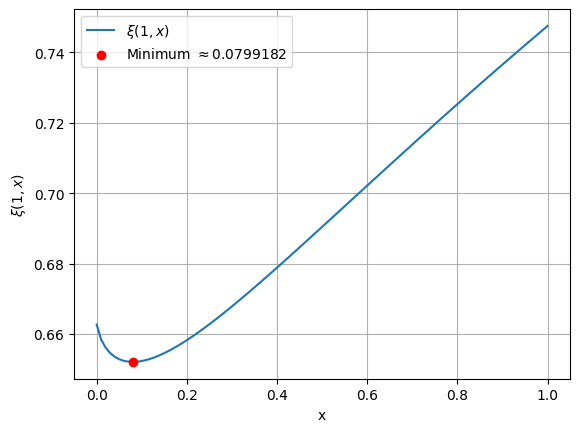
A relevant question, having Corollary 1.7 in mind, is whether there exists a “worst” (resp. “best”) ratio b/ab/a for which the average coverage density ξ⁡(1,b/a)\xi(1,b/a) is smallest (resp. largest). As we see in Lemma 1.10, there exists a unique worst ratio, minimising the average coverage density x↦ξ⁡(1,x)x\mapsto\xi(1,x) for x∈[0,1]x\in[0,1], and surprisingly, we find that x↦ξ⁡(1,x)x\mapsto\xi(1,x) is not strictly increasing. Moreover, since x↦ξ⁡(1,x)x\mapsto\xi(1,x) only has one extremum point, which is a minimum on (0,1)(0,1), the “best” ratio must therefore be at 00 or 11, values which are already known from [31] and [33], concluding that the “best” case is b/a=1b/a=1.

Lemma 1.10.

The function x↦ξ⁡(1,x)x\mapsto\xi(1,x) defined on [0,1][0,1] has a unique minimiser x∗∈(0,1)x^{\ast}\in(0,1) such that ξ⁡(1,x∗)=infx∈[0,1]ξ⁡(1,x)\xi(1,x^{*})=\inf_{x\in[0,1]}\xi(1,x).

From available analytical tools, finding a closed form for the minimiser does not seem possible. However, numerical evaluation shows x∗≈0.07991824x^{\ast}\approx 0.07991824, as we can also see in Figure 5.

Refer to caption
(a) Plot of x↦ξ⁡(1,x)x\mapsto\xi(1,x) for x∈[0,1]x\in[0,1].
Refer to caption
(b) Plot of the derivative x↦dd​x​ξ​(1,x)x\mapsto\tfrac{\,\mathrm{d}}{\,\mathrm{d}x}\xi(1,x) for x∈(0,1]x\in(0,1].
Figure 5. Finding the worst trapezium.

At first, it seems surprising that x↦ξ⁡(1,x)x\mapsto\xi(1,x) from Corollary 1.7 is not strictly increasing. The cases of x=0x=0 and x=1x=1 were known, since those are precisely the jamming limits from [31] and [33]. Hence, one could be tempted to think that we should expect to see a strictly increasing function x↦ξ⁡(1,x)x\mapsto\xi(1,x). However, after simulations (Figure 7) and plotting the closed form of the function (Figure 5), it seems clearer why such a shape would occur. Indeed, if our deposited objects are triangles, we will almost surely alternate between triangles with their base on the upper line of the substrate, and triangles with their base on the lower line of the substrate (see Figure 6(a)). However, as soon as the value xx is strictly larger than 00, there is a positive probability of having two trapeziums next to each other, both having their (longer) base on the same line of the substrate (see Figure 6(b)). This can potentially leave large unusable gaps, and this provides a geometric mechanism explaining the initial decrease for the jamming limit.

(a) Triangles
(b) Trapeziums
Figure 6. Big gaps appearing once triangles are replaced with trapeziums.
Refer to caption
Figure 7. Simulation of x↦ξ⁡(1,x)x\mapsto\xi(1,x) for x∈[0,1]x\in[0,1].

In addition to plotting the function ξ⁡(1,x)\xi(1,x) from Corollary 1.7, we ran a simulation of our model. The precise values of xx in the simulations went from 00 to 11 with a step size of 0.010.01. For each particular value of xx, we ran 500500 simulations, with the strip length set to 50005000. Simulation results are shown in Figure 7. Clearly, the illustrative MC approximation aligns very well with the function shown in Figure 5(a).

1.4. Open Problems

Below, we list some open problems related to those considered in this paper, which seem appropriate for future work.

  • •

    A CLT for the variables TxT_{x} and PxP_{x}, whenever a>ba>b, and a quantitative bound via a Stein’s argument in the total-variation distance or the Wasserstein distance.

  • •

    Finding whether λ2​(a,b)\lambda_{2}(a,b) admits an explicit integral representation analogous to λ⁡(a,b)\lambda(a,b).

  • •

    While we have shown that there exists a unique minimiser for x↦ξ⁡(1,x)x\mapsto\xi(1,x) on [0,1][0,1], an open problem is finding a closed analytical form for the minimiser x∗x^{*}. Due to the very complex form of ξ⁡(1,x)\xi(1,x), such an analytical closed form for x∗x^{*} seems out of reach, but it is an open problem.

2. Proofs

2.1. Recursive equations for regularity

Lemma 2.1.

For η\eta defined in (6), it follows that η⁡(x)=0\eta(x)=0 for x∈[0,(a+b)/2)x\in[0,(a+b)/2), η⁡(x)=1/2\eta(x)=1/2 for [(a+b)/2,a)[(a+b)/2,a), η⁡(a)=1\eta(a)=1 and

(13) η⁡(x)=1+1x−a​(∫0x−aη⁡(t)​𝑑t+∫0x−a+b2η⁡(t)​𝑑t), for all ​x>a,\eta(x)=1+\frac{1}{x-a}\bigg(\int_{0}^{x-a}\eta(t)\,\mathrm{d}t+\int_{0}^{x-\tfrac{a+b}{2}}\eta(t)\,\mathrm{d}t\bigg),\quad\text{ for all }x>a,

where η\eta is a non-decreasing function on (0,∞)(0,\infty), and continuous on (a,∞)(a,\infty), specifically η\eta is locally absolutely continuous on (a,∞)(a,\infty).

Proof of Lemma 2.1.

Recall the definition of PxP_{x} and TxT_{x} and how we deposit the trapeziums using the random sequential adsorption model. Under the 𝒰​𝒟​𝒜\mathcal{UDA}, we let τ∼𝒰⁡(0,2​x−2​a)\tau\sim\mathcal{U}(0,2x-2a), which yields a self-recursive relation which works in the case where x≥(3​a−b)/2x\geq(3a-b)/2. This case is covered in (16) below. However, we will first consider the values of xx up to (3​a−b)/2(3a-b)/2, since we can determine directly the exact number of possible deposited trapeziums.

We start by finding the initial values of ν\nu and μ\mu for x<(3​a+b)/2x<(3a+b)/2, by counting the number of possibilities for deposited trapeziums. Note that we need the initial values of μ\mu and ν\nu only for x<(3​a−b)/2x<(3a-b)/2. However, in the procedure that follows, we build up those values with steps of particular sizes, and we do that until we are sure that we crossed over (3​a−b)/2(3a-b)/2. When x<(a+b)/2x<(a+b)/2, it follows directly from definition that 𝒯(a+b)/2\mathcal{T}_{(a+b)/2} cannot fit on either 𝒯x\mathcal{T}_{x} or 𝒫x\mathcal{P}_{x}, and hence η⁡(x)=0\eta(x)=0 for x∈(0,(a+b)/2)x\in(0,(a+b)/2). Next, for x∈[(a+b)/2,a)x\in[(a+b)/2,a), we have that Px=0P_{x}=0 since 𝒯(a+b)/2\mathcal{T}_{(a+b)/2} cannot fit on 𝒫x\mathcal{P}_{x}, and Tx=1T_{x}=1 since we will always be able to fit one and only one 𝒯(a+b)/2\mathcal{T}_{(a+b)/2} on 𝒯x\mathcal{T}_{x}. This yields that η⁡(x)=1/2\eta(x)=1/2 for all x∈[(a+b)/2,a)x\in[(a+b)/2,a). Consider now x∈[a,a+b)x\in[a,a+b). In this case Tx=1T_{x}=1 (resp. Px=1P_{x}=1) since we can fit one and only one 𝒯(a+b)/2\mathcal{T}_{(a+b)/2} on 𝒯x\mathcal{T}_{x} (resp. 𝒫x\mathcal{P}_{x}). Hence, η⁡(x)=1\eta(x)=1 for all x∈[a,a+b)x\in[a,a+b). Notice that a+ba+b is not necessarily greater than (3​a−b)/2(3a-b)/2, so we have to go further.

Let now x∈[a+b,(3a+b)/2)x\in[a+b,(3a+b)/2). In this case, it follows that Tx=1T_{x}=1 for all x∈[a+b,(3a+b)/2)x\in[a+b,(3a+b)/2), and hence it suffices to calculate PxP_{x}. Let τ∼𝒰⁡(0,2​x−2​a)\tau\sim\mathcal{U}(0,2x-2a), implying by (5) that

(14) Px=2𝟙{τ∈(0,x−a−b)}+𝟙{τ∈(x−a−b,x−a)}+𝟙{τ∈(x−a,x−a+b)}+2𝟙{τ∈(x−a+b,2x−2a)} a.s.P_{x}=2\mathds{1}_{\{\tau\in(0,x-a-b)\}}+\mathds{1}_{\{\tau\in(x-a-b,x-a)\}}+\mathds{1}_{\{\tau\in(x-a,x-a+b)\}}+2\mathds{1}_{\{\tau\in(x-a+b,2x-2a)\}}\,\text{ a.s}.

Hence, by the law of total expectation 𝔼⁡[XT]=𝔼⁡[𝔼⁡[Xt|T=t]]\mathds{E}[X_{T}]=\mathds{E}[\mathds{E}[X_{t}|T=t]], it follows that

(15) μ⁡(x)=𝔼⁡[Px]=12​x−2​a​(∫0x−a−b2​𝑑t+∫x−a−bx−a+b𝑑t+∫x−a+b2​x−2​a2​𝑑t)=1+x−a−bx−a.\mu(x)=\mathds{E}[P_{x}]=\frac{1}{2x-2a}\bigg(\int_{0}^{x-a-b}2\,\mathrm{d}t+\int_{x-a-b}^{x-a+b}\,\mathrm{d}t+\int_{x-a+b}^{2x-2a}2\,\mathrm{d}t\bigg)=1+\frac{x-a-b}{x-a}.

Altogether, we therefore have that η⁡(x)=1+(x−a−b)/(2​x−2​a)\eta(x)=1+(x-a-b)/(2x-2a) for all x∈[a+b,(3a+b)/2)x\in[a+b,(3a+b)/2).

If x>(3​a−b)/2x>(3a-b)/2, it follows from Definition 1.2 of 𝒰​𝒟​𝒜\mathcal{UDA}, that

(16) Px=1+𝟙{τ∈(0,x−a)}(Pτ+Tx−τ−a+b2)+𝟙{τ∈(x−a,2x−2a)}(Ttτ+Px−tτ−a+b2) a.s. and,Tx=1+𝟙{τ∈(0,x−3​a−b2)}(Tτ+a−b2+Tx−τ−a)+𝟙{τ∈(x−3​a−b2,2x−2a)}(Ptτ+Px−tτ−a+b2) a.s.,\displaystyle\begin{aligned} P_{x}&=1+\mathds{1}_{\{\tau\in(0,x-a)\}}\bigg(P_{\tau}+T_{x-\tau-\tfrac{a+b}{2}}\bigg)+\mathds{1}_{\{\tau\in(x-a,2x-2a)\}}\bigg(T_{t_{\tau}}+P_{x-t_{\tau}-\tfrac{a+b}{2}}\bigg)\,\text{ a.s. and},\\ T_{x}&=1+\mathds{1}_{\big\{\tau\in\big(0,x-\tfrac{3a-b}{2}\big)\big\}}\bigg(T_{\tau+\tfrac{a-b}{2}}+T_{x-\tau-a}\bigg)+\mathds{1}_{\big\{\tau\in\big(x-\tfrac{3a-b}{2},2x-2a\big)\big\}}\bigg(P_{t_{\tau}}+P_{x-t_{\tau}-\tfrac{a+b}{2}}\bigg)\,\text{ a.s.},\end{aligned}

where tτ=τ+(3​a−b)/2−xt_{\tau}=\tau+(3a-b)/2-x, as illustrated in Figure 8. For all x≥(3​a+b)/2>(3​a−b)/2x\geq(3a+b)/2>(3a-b)/2 we can find η⁡(x)\eta(x) by the recursive relationship in (16). By the useful rule 𝔼⁡[XT]=𝔼⁡[𝔼⁡[Xt|T=t]]\mathds{E}[X_{T}]=\mathds{E}[\mathds{E}[X_{t}|T=t]] and change of variables, it follows from (16) that

(17) μ⁡(x)=1+12​x−2​a​(∫0x−aμ⁡(t)+ν⁡(x−t−a+b2)​𝑑t+∫a−b2x−a+b2ν⁡(t)+μ⁡(x−t−a+b2)​𝑑t)=1+1x−a​(∫0x−aμ⁡(t)​dt+∫a−b2x−a+b2ν⁡(t)​dt).\displaystyle\begin{aligned} \mu(x)&=1+\frac{1}{2x-2a}\bigg(\int_{0}^{x-a}\mu(t)+\nu\big(x-t-\tfrac{a+b}{2}\big)\,\mathrm{d}t+\int_{\tfrac{a-b}{2}}^{x-\tfrac{a+b}{2}}\nu(t)+\mu\big(x-t-\tfrac{a+b}{2}\big)\,\mathrm{d}t\bigg)\\ &=1+\frac{1}{x-a}\bigg(\int_{0}^{x-a}\mu(t)\,\mathrm{d}t+\int_{\tfrac{a-b}{2}}^{x-\tfrac{a+b}{2}}\nu(t)\,\mathrm{d}t\bigg).\end{aligned}

Similarly, it follows from (16) that

(18) ν⁡(x)=1+12​x−2​a​(∫0x−3​a−b2ν⁡(t+a−b2)+ν⁡(x−t−a)​𝑑t+∫0x−a+b2μ⁡(t)+μ⁡(x−t−a+b2)​𝑑t)=1+1x−a​(∫a−b2x−aν⁡(t)​dt+∫0x−a+b2μ⁡(t)​dt).\displaystyle\begin{aligned} \nu(x)&=1+\frac{1}{2x-2a}\bigg(\int_{0}^{x-\tfrac{3a-b}{2}}\nu\big(t+\tfrac{a-b}{2}\big)+\nu(x-t-a)\,\mathrm{d}t+\int_{0}^{x-\tfrac{a+b}{2}}\mu(t)+\mu\big(x-t-\tfrac{a+b}{2}\big)\,\mathrm{d}t\bigg)\\ &=1+\frac{1}{x-a}\bigg(\int_{\tfrac{a-b}{2}}^{x-a}\nu(t)\,\mathrm{d}t+\int_{0}^{x-\tfrac{a+b}{2}}\mu(t)\,\mathrm{d}t\bigg).\end{aligned}

Note that ν⁡(x)=0\nu(x)=0 for all x∈(0,(a−b)/2)x\in(0,(a-b)/2), since we cannot fit 𝒯(a+b)/2\mathcal{T}_{(a+b)/2} inside 𝒯(a−b)/2\mathcal{T}_{(a-b)/2}. Thus,

(19) η⁡(x)=1+1x−a​(∫0x−aη⁡(t)​𝑑t+∫0x−a+b2η⁡(t)​𝑑t), for all ​x≥3​a+b2.\eta(x)=1+\frac{1}{x-a}\bigg(\int_{0}^{x-a}\eta(t)\,\mathrm{d}t+\int_{0}^{x-\tfrac{a+b}{2}}\eta(t)\,\mathrm{d}t\bigg),\quad\text{ for all }x\geq\frac{3a+b}{2}.

By using the values for η⁡(x)\eta(x) when x∈(0,a+b)x\in(0,a+b), one can show that the form η⁡(x)=1+(x−a−b)/(2​x−2​a)\eta(x)=1+(x-a-b)/(2x-2a) for all x∈[a+b,(3a+b)/2)x\in[a+b,(3a+b)/2) found above, corresponds to plugging the initial η\eta values into (19), concluding that (19) holds for all x>a+bx>a+b. The similar approach holds for x∈(a,a+b)x\in(a,a+b), since η⁡(x)=0\eta(x)=0 for all x<(a+b)/2x<(a+b)/2. Hence, (19) holds for all x>ax>a.

xxtttttt++x−t−bx-t-bx−t−ax-t-a
(a) Trapezium 𝒯(a+b)/2\mathcal{T}_{(a+b)/2} arriving on 𝒫x\mathcal{P}_{x} with base up.
t−a−b2t-\frac{a-b}{2}xxt−a−b2t-\frac{a-b}{2}t+a−b2t+\frac{a-b}{2}++x−t−a+b2x-t-\frac{a+b}{2}x−t−a+b2x-t-\frac{a+b}{2}
(b) Trapezium 𝒯(a+b)/2\mathcal{T}_{(a+b)/2} arriving on 𝒫x\mathcal{P}_{x} with base down.
x+a−b2x+\frac{a-b}{2}t−a−b2t-\frac{a-b}{2}t+a−b2t+\frac{a-b}{2}t−a−b2t-\frac{a-b}{2}++x−t−bx-t-bx−t−ax-t-a
(c) Trapezium 𝒯(a+b)/2\mathcal{T}_{(a+b)/2} arriving on 𝒯x\mathcal{T}_{x} with base up.
ttx−a−b2x-\frac{a-b}{2}tttt++x−t−a+b2x-t-\frac{a+b}{2}x−t−a+b2x-t-\frac{a+b}{2}
(d) Trapezium 𝒯(a+b)/2\mathcal{T}_{(a+b)/2} arriving on 𝒯x\mathcal{T}_{x} with base down.
Figure 8. Illustration of all the possible scenarios of the trapezium 𝒯(a+b)/2\mathcal{T}_{(a+b)/2} arriving on strips 𝒫x\mathcal{P}_{x} and 𝒯x\mathcal{T}_{x} (introduced in Figure 3). After a trapezium arrives, the original strip decomposes into two smaller strips that are again of the two types introduced in Figure 3.

We can now show that η\eta is continuous on (a,∞)(a,\infty). Define the indefinite integral J⁡(z)≔∫0zη⁡(t)​𝑑tJ(z)\coloneqq\int_{0}^{z}\eta(t)\,\mathrm{d}t, for z≥0z\geq 0. Since η\eta is (piecewise) bounded on bounded intervals, JJ is locally Lipschitz-continuous, and hence continuous, on [0,∞)[0,\infty). For x>ax>a we may rewrite (13) as η⁡(x)=1+(J⁡(x−a)+J⁡(x−(a+b)/2))/(x−a)\eta(x)=1+(J(x-a)+J(x-(a+b)/2))/(x-a). Here x↦x−ax\mapsto x-a and x↦x−(a+b)/2x\mapsto x-(a+b)/2 are continuous on (a,∞)(a,\infty), JJ is continuous on [0,∞)[0,\infty), and the denominator x−ax-a never vanishes on (a,∞)(a,\infty). Therefore, η\eta is continuous on (a,∞)(a,\infty).

Next, we prove that x↦η⁡(x)x\mapsto\eta(x) is non-decreasing on (0,∞)(0,\infty). Since η\eta is locally bounded, JJ is locally absolutely continuous on [0,∞)[0,\infty). Moreover, for all x>ax>a, we have η⁡(x)=1+(J⁡(x−a)+J⁡(x−(a+b)/2))/(x−a)\eta(x)=1+(J(x-a)+J(x-(a+b)/2))/(x-a), as discussed above. Therefore, it follows that η\eta is locally absolutely continuous on (a,∞)(a,\infty). In particular, since J′​(z)=η​(z)J^{\prime}(z)=\eta(z) for almost every z>0z>0, differentiation of the preceding identity yields, for almost every x>ax>a,

(20) dd​x​η​(x)=−1(x−a)2​(∫0x−aη⁡(t)​𝑑t+∫0x−a+b2η⁡(t)​𝑑t)+1x−a​(η⁡(x−a)+η⁡(x−a+b2)).\frac{\,\mathrm{d}}{\,\mathrm{d}x}\eta(x)=-\frac{1}{(x-a)^{2}}\bigg(\int_{0}^{x-a}\eta(t)\,\mathrm{d}t+\int_{0}^{x-\tfrac{a+b}{2}}\eta(t)\,\mathrm{d}t\bigg)+\frac{1}{x-a}\bigg(\eta(x-a)+\eta\bigl(x-\tfrac{a+b}{2}\bigr)\bigg).

Furthermore,

η⁡(x−a)x−a=1(x−a)2​∫0x−aη⁡(x−a)​𝑑t,andη⁡(x−a+b2)x−a=1(x−a)2​∫a−b2x−a+b2η⁡(x−a+b2)​𝑑t.\frac{\eta(x-a)}{x-a}=\frac{1}{(x-a)^{2}}\int_{0}^{x-a}\eta(x-a)\,\mathrm{d}t,\quad\text{and}\quad\frac{\eta\bigl(x-\tfrac{a+b}{2}\bigr)}{x-a}=\frac{1}{(x-a)^{2}}\int_{\tfrac{a-b}{2}}^{x-\tfrac{a+b}{2}}\eta\bigl(x-\tfrac{a+b}{2}\bigr)\,\mathrm{d}t.

Since η⁡(t)=0\eta(t)=0 for t∈(0,(a−b)/2)t\in(0,(a-b)/2), we therefore obtain, for almost every x>ax>a,

(21) dd​x​η​(x)=1(x−a)2​(∫0x−a(η⁡(x−a)−η⁡(t))​𝑑t+∫a−b2x−a+b2(η⁡(x−a+b2)−η⁡(t))​𝑑t).\frac{\,\mathrm{d}}{\,\mathrm{d}x}\eta(x)=\frac{1}{(x-a)^{2}}\bigg(\int_{0}^{x-a}\bigl(\eta(x-a)-\eta(t)\bigr)\,\mathrm{d}t+\int_{\tfrac{a-b}{2}}^{x-\tfrac{a+b}{2}}\bigl(\eta\bigl(x-\tfrac{a+b}{2}\bigr)-\eta(t)\bigr)\,\mathrm{d}t\bigg).

By the initial values established above, x↦η⁡(x)x\mapsto\eta(x) is non-decreasing on (0,a](0,a]. Moreover, η≥0\eta\geq 0, and hence (13) shows that η⁡(x)≥1=η⁡(a)\eta(x)\geq 1=\eta(a) for every x>ax>a. Thus, in order to extend the monotonicity beyond aa, it suffices, in view of (21), to verify that

(22) η⁡(x−a)−η⁡(t)≥0for all ​t∈(0,x−a),andη⁡(x−a+b2)−η⁡(t)≥0for all ​t∈(a−b2,x−a+b2).\eta(x-a)-\eta(t)\geq 0\quad\text{for all }t\in(0,x-a),\quad\text{and}\quad\eta\bigl(x-\tfrac{a+b}{2}\bigr)-\eta(t)\geq 0\quad\text{for all }t\in\bigl(\tfrac{a-b}{2},x-\tfrac{a+b}{2}\bigr).

Since η\eta is non-decreasing on (0,a](0,a], both equations in (22) hold whenever x−(a+b)/2<ax-(a+b)/2<a, that is, whenever a<x<a+(a+b)/2=(3​a+b)/2a<x<a+(a+b)/2=(3a+b)/2. Indeed, since (a+b)/2≤a(a+b)/2\leq a, we also have x−a≤x−(a+b)/2<ax-a\leq x-(a+b)/2<a. Hence η′​(x)≥0\eta^{\prime}(x)\geq 0 for almost every x∈(a,(3​a+b)/2)x\in(a,(3a+b)/2). Since η\eta is absolutely continuous on every compact subinterval of (a,∞)(a,\infty), it follows that η\eta is non-decreasing on (a,(3​a+b)/2)(a,(3a+b)/2). Together with the initial values and the fact that η⁡(x)≥η⁡(a)\eta(x)\geq\eta(a) for x>ax>a, this shows that η\eta is non-decreasing on (0,(3​a+b)/2)(0,(3a+b)/2), i.e. on (0,a+(a+b)/2)(0,a+(a+b)/2).

We now proceed by induction. For n≥1n\geq 1, let the nn-th induction hypothesis be

(23) x↦η⁡(x)​ is non-decreasing on ​(0,a+n​a+b2).x\mapsto\eta(x)\text{ is non-decreasing on }\biggl(0,a+n\frac{a+b}{2}\biggr).

The preceding argument proves the case n=1n=1. Assume that (23) holds for some n≥1n\geq 1. Let a+n⁡(a+b)/2<x<a+(n+1)​(a+b)/2a+n(a+b)/2<x<a+(n+1)(a+b)/2. Then, x−(a+b)/2<a+n⁡(a+b)/2x-(a+b)/2<a+n(a+b)/2. Moreover, since (a+b)/2≤a(a+b)/2\leq a, it follows that x−a≤x−(a+b)/2<a+n⁡(a+b)/2x-a\leq x-(a+b)/2<a+n(a+b)/2. Thus, by the induction hypothesis, (22) holds for this xx. It follows from (21) that η′​(x)≥0\eta^{\prime}(x)\geq 0 for almost every x∈(a+n⁡(a+b)/2,a+(n+1)​(a+b)/2)x\in(a+n(a+b)/2,a+(n+1)(a+b)/2). Since η\eta is locally absolutely continuous on (a,∞)(a,\infty), for any a+n⁡(a+b)/2<u<v<a+(n+1)​(a+b)/2a+n(a+b)/2<u<v<a+(n+1)(a+b)/2, we have η⁡(v)−η⁡(u)=∫uvη′​(x)​𝑑x≥0\eta(v)-\eta(u)=\int_{u}^{v}\eta^{\prime}(x)\,\mathrm{d}x\geq 0. Hence η\eta is non-decreasing on this interval. Since η\eta is continuous on (a,∞)(a,\infty), this monotonicity joins continuously with the induction hypothesis at a+n⁡(a+b)/2a+n(a+b)/2, and therefore (23) holds with nn replaced by n+1n+1.

By induction, x↦η⁡(x)x\mapsto\eta(x) is non-decreasing on (0,∞)(0,\infty), completing the proof. ∎

2.2. Exact parking constant

Lemma 2.2.

For all 0≤b≤a<∞0\leq b\leq a<\infty such that a>0a>0, and η\eta defined in (6), it follows that

(24) limx→∞η⁡(x)x=λ⁡(a,b)=12​∫0∞(2+e−t​b−e−t​a)​exp⁡(∫0t−2+e−s(a+b)/2+e−a​ss​𝑑s)​𝑑t∈(0,∞).\lim_{x\to\infty}\frac{\eta(x)}{x}=\lambda(a,b)=\frac{1}{2}\int_{0}^{\infty}(2+e^{-tb}-e^{-ta})\exp\bigg(\int_{0}^{t}\frac{-2+e^{-s(a+b)/2}+e^{-as}}{s}\,\mathrm{d}s\bigg)\,\mathrm{d}t\in(0,\infty).

For the proof of Lemma 2.2, we define the “aa-truncated” Laplace transform of η\eta, by

(25) F⁡(x)≔∫a∞η⁡(s)​e−s​x​𝑑s,F(x)\coloneqq\int_{a}^{\infty}\eta(s)e^{-sx}\,\mathrm{d}s,

which is well-defined, since s↦η⁡(s)​e−s​x∈ℒ1​((a,∞))s\mapsto\eta(s)e^{-sx}\in\mathcal{L}^{1}((a,\infty)) for all x>0x>0.

Proof of Lemma 2.2.

From Lemma 2.1 we have that η\eta is locally absolutely continuous on (a,∞)(a,\infty), and hence by (20), it follows for almost every x>ax>a, that

(26) η⁡(x)+(x−a)​η′​(x)=1+η⁡(x−a)+η⁡(x−a+b2).\eta(x)+(x-a)\eta^{\prime}(x)=1+\eta(x-a)+\eta\big(x-\tfrac{a+b}{2}\big).

Note that s↦(η⁡(s)+(s−a)​η′​(s))​e−s​x∈ℒ1​((a,∞))s\mapsto(\eta(s)+(s-a)\eta^{\prime}(s))e^{-sx}\in\mathcal{L}^{1}((a,\infty)) for all x>0x>0. Indeed, by (26) it is equivalent to show that s↦(1+η⁡(s−a)+η⁡(s−(a+b)/2))​e−s​x∈ℒ1​((a,∞))s\mapsto(1+\eta(s-a)+\eta(s-(a+b)/2))e^{-sx}\in\mathcal{L}^{1}((a,\infty)) for all x>0x>0, which follows directly from the linear growth of η\eta as shown in Remark 1.4. Thus, (s−a)​η′​(s)​e−s​x∈ℒ1​((a,∞))(s-a)\eta^{\prime}(s)e^{-sx}\in\mathcal{L}^{1}((a,\infty)) by Remark 1.4 and since η⁡(s)\eta(s) is positive. Hence, it follows from (26) and Remark 1.4 that

(27) F⁡(x)+∫a∞(s−a)​η′​(s)​e−s​x​𝑑s=∫a∞e−s​x​𝑑s+∫a∞η⁡(s−a)​e−s​x​𝑑s+∫a∞η⁡(s−a+b2)​e−s​x​𝑑s,F(x)+\int_{a}^{\infty}(s-a)\eta^{\prime}(s)e^{-sx}\,\mathrm{d}s=\int_{a}^{\infty}e^{-sx}\,\mathrm{d}s+\int_{a}^{\infty}\eta(s-a)e^{-sx}\,\mathrm{d}s+\int_{a}^{\infty}\eta(s-\tfrac{a+b}{2})e^{-sx}\,\mathrm{d}s,

for all x>0x>0. Each integral in (27) is finite and well-defined, as argued above. By integration by parts, each integral in (27) can be written in terms of F⁡(x)F(x). Since η\eta is locally absolutely continuous on (a,∞)(a,\infty), we may apply integration by parts on [a+ε,R][a+\varepsilon,R], for every ε>0\varepsilon>0 and R>a+εR>a+\varepsilon. Letting ε↓0\varepsilon\downarrow 0 and R→∞R\to\infty, the boundary terms vanish by the linear growth bound from Remark 1.4, and hence

(28) I1​(x)≔∫a∞(s−a)​η′​(s)​e−s​x​𝑑s=x​∫a∞s​η​(s)​e−s​x​𝑑s−(1+a​x)​F​(x).\displaystyle I_{1}(x)\coloneqq\int_{a}^{\infty}(s-a)\eta^{\prime}(s)e^{-sx}\,\mathrm{d}s=x\int_{a}^{\infty}s\eta(s)e^{-sx}\,\mathrm{d}s-(1+ax)F(x).

Note, that s↦η⁡(s)​e−s​x∈ℒ1​((a,∞))s\mapsto\eta(s)e^{-sx}\in\mathcal{L}^{1}((a,\infty)) for all x>0x>0 and |dd​x​η​(s)​e−s​x|=|s​η​(s)​e−s​x|≤s​η​(s)​e−s|\tfrac{\,\mathrm{d}}{\,\mathrm{d}x}\eta(s)e^{-sx}|=|s\eta(s)e^{-sx}|\leq s\eta(s)e^{-s} for all x≥1x\geq 1, where s↦s​η​(s)​e−s∈ℒ1​((a,∞))s\mapsto s\eta(s)e^{-s}\in\mathcal{L}^{1}((a,\infty)). If we instead consider x∈(0,1)x\in(0,1), then we may fix x0>0x_{0}>0 and consider all x∈[x0,1)x\in[x_{0},1), for which |dd​xη(s)e−s​x|≤sη(s)e−sx0/2|\tfrac{\,\mathrm{d}}{\,\mathrm{d}x}\eta(s)e^{-sx}|\leq s\eta(s)e^{-sx_{0}/2}, where s↦sη(s)e−sx0/2∈ℒ1((a,∞))s\mapsto s\eta(s)e^{-sx_{0}/2}\in\mathcal{L}^{1}((a,\infty)). Since x0>0x_{0}>0 is arbitrary, we have that |dd​x​η​(s)​e−s​x||\tfrac{\,\mathrm{d}}{\,\mathrm{d}x}\eta(s)e^{-sx}| is in ℒ1​((,,,))\mathcal{L}^{1}((a,\infty)) for all x>0x>0. Hence, when calculating F′​(x)F^{\prime}(x), we can change the order of integration and differentiation, implying that F′(x)=−∫a∞sη(s)e−s​xdsF^{\prime}(x)=-\int_{a}^{\infty}s\eta(s)e^{-sx}\,\mathrm{d}s for all x>0x>0. Thus,

(29) I1​(x)=−x​F′​(x)−(1+a​x)​F​(x), for all ​x>0.I_{1}(x)=-xF^{\prime}(x)-(1+ax)F(x),\quad\text{ for all }x>0.

Next, we get directly that I2​(x)≔∫a∞e−s​x​𝑑s=e−a​x/xI_{2}(x)\coloneqq\int_{a}^{\infty}e^{-sx}\,\mathrm{d}s=e^{-ax}/x for all x>0x>0. By change of variables, it follows that

(30) I3​(x)\displaystyle I_{3}(x) ≔∫a∞η⁡(s−a)​e−s​x​𝑑s=e−a​x​∫0∞η⁡(s)​e−s​x​𝑑s\displaystyle\coloneqq\int_{a}^{\infty}\eta(s-a)e^{-sx}\,\mathrm{d}s=e^{-ax}\int_{0}^{\infty}\eta(s)e^{-sx}\,\mathrm{d}s
(31) =e−a​x​(12​∫a+b2ae−s​x​𝑑s+F⁡(x))=e−a​x​(12​x​(e−x⁡(a+b2)−e−x​a)+F⁡(x)).\displaystyle=e^{-ax}\bigg(\frac{1}{2}\int_{\tfrac{a+b}{2}}^{a}e^{-sx}\,\mathrm{d}s+F(x)\bigg)=e^{-ax}\bigg(\frac{1}{2x}\bigg(e^{-x\big(\tfrac{a+b}{2}\big)}-e^{-xa}\bigg)+F(x)\bigg).

Similarly, it follows that

(32) I4​(x)≔∫a∞η⁡(s−a+b2)​e−s​x​𝑑s=e−(a+b2)​x​(12​x​(e−x⁡(a+b2)−e−x​a)+F⁡(x)).I_{4}(x)\coloneqq\int_{a}^{\infty}\eta\big(s-\tfrac{a+b}{2}\big)e^{-sx}\,\mathrm{d}s=e^{-\big(\tfrac{a+b}{2}\big)x}\bigg(\frac{1}{2x}\bigg(e^{-x\big(\tfrac{a+b}{2}\big)}-e^{-xa}\bigg)+F(x)\bigg).

Using (27), together with I1​(x)I_{1}(x), I2​(x)I_{2}(x), I3​(x)I_{3}(x) and I4​(x)I_{4}(x), it follows that

(33) F′​(x)+F⁡(x)​(a+e−x⁡(a+b2)x+e−a​xx)=12​x2​(e−2​x​a−2​e−x​a−e−x⁡(a+b)), for all ​x>0.F^{\prime}(x)+F(x)\left(a+\frac{e^{-x\big(\tfrac{a+b}{2}\big)}}{x}+\frac{e^{-ax}}{x}\right)=\frac{1}{2x^{2}}\bigg(e^{-2xa}-2e^{-xa}-e^{-x(a+b)}\bigg),\quad\text{ for all }x>0.

Next, define ℐ\mathcal{I} as follows:

(34) ℐ⁡(x)≔exp⁡{∫1x(a​s+e−s⁡(a+b2)+e−s​a)​d​ss}, for all ​x>0.\mathcal{I}(x)\coloneqq\exp\left\{\int_{1}^{x}\bigg(as+e^{-s\big(\tfrac{a+b}{2}\big)}+e^{-sa}\bigg)\frac{\,\mathrm{d}s}{s}\right\},\quad\text{ for all }x>0.

By definition of ℐ\mathcal{I} and (33), we see that

(35) dd​x​F​(x)​ℐ​(x)=F′​(x)​ℐ​(x)+F⁡(x)​ℐ​(x)x​(a​x+e−x⁡(a+b2)+e−a​x)=ℐ⁡(x)2​x2​(e−2​x​a−2​e−x​a−e−x⁡(a+b)),\frac{\,\mathrm{d}}{\,\mathrm{d}x}F(x)\mathcal{I}(x)=F^{\prime}(x)\mathcal{I}(x)+\frac{F(x)\mathcal{I}(x)}{x}\left(ax+e^{-x\big(\tfrac{a+b}{2}\big)}+e^{-ax}\right)=\frac{\mathcal{I}(x)}{2x^{2}}\left(e^{-2xa}-2e^{-xa}-e^{-x(a+b)}\right),

for all x>0x>0. Next, we show that the right-hand side of (35) belongs to ℒ1​((,,,))\mathcal{L}^{1}((0,\infty)). We consider separately the regions (0,1](0,1] and [1,∞)[1,\infty). First, let x∈(0,1]x\in(0,1]. Recall the definition of ℐ\mathcal{I}. Using the elementary inequality e−u≥1−ue^{-u}\geq 1-u, we obtain e−s(a+b)/2+e−a​s≥2−((a+b)/2+a)se^{-s(a+b)/2}+e^{-as}\geq 2-((a+b)/2+a)s for all s>0s>0. Since x≤1x\leq 1, reversing the limits of integration yields

∫1xe−s(a+b)/2+e−a​ss​𝑑s\displaystyle\int_{1}^{x}\frac{e^{-s(a+b)/2}+e^{-as}}{s}\,\mathrm{d}s ≤∫1x(2s−a+b2−a)​𝑑s=2​log⁡x−(a+b2+a)​(x−1).\displaystyle\leq\int_{1}^{x}\left(\frac{2}{s}-\frac{a+b}{2}-a\right)\,\mathrm{d}s=2\log x-\left(\frac{a+b}{2}+a\right)(x-1).

Consequently,

log⁡ℐ⁡(x)\displaystyle\log\mathcal{I}(x) ≤a⁡(x−1)+2​log​x−(a+b2+a)​(x−1)=2​log​x+a+b2​(1−x)≤2​log​x+a+b2.\displaystyle\leq a(x-1)+2\log x-\left(\frac{a+b}{2}+a\right)(x-1)=2\log x+\frac{a+b}{2}(1-x)\leq 2\log x+\frac{a+b}{2}.

Hence, ℐ⁡(x)≤e(a+b)/2​x2\mathcal{I}(x)\leq e^{(a+b)/2}x^{2} for all x∈(0,1]x\in(0,1]. It follows for all x∈(0,1]x\in(0,1], that

|ℐ⁡(x)2​x2​(e−2​a​x−2​e−a​x−e−(a+b)​x)|≤e(a+b)/22​(e−2​a​x+2​e−a​x+e−(a+b)​x)≤2​e(a+b)/2,\displaystyle\left|\frac{\mathcal{I}(x)}{2x^{2}}\left(e^{-2ax}-2e^{-ax}-e^{-(a+b)x}\right)\right|\leq\frac{e^{(a+b)/2}}{2}\left(e^{-2ax}+2e^{-ax}+e^{-(a+b)x}\right)\leq 2e^{(a+b)/2},

where we used a,b>0a,b>0. Therefore,

(36) ∫01|ℐ⁡(x)2​x2​(e−2​a​x−2​e−a​x−e−(a+b)​x)|​𝑑x<∞.\int_{0}^{1}\left|\frac{\mathcal{I}(x)}{2x^{2}}\left(e^{-2ax}-2e^{-ax}-e^{-(a+b)x}\right)\right|\,\mathrm{d}x<\infty.

It remains to consider x≥1x\geq 1. Since x↦∫1x(e−s(a+b)/2+e−a​s)s−1dsx\mapsto\int_{1}^{x}(e^{-s(a+b)/2}+e^{-as})s^{-1}\,\mathrm{d}s is an increasing function and ∫1∞e−c​s​s−1​𝑑s=−Ei⁡(−c)\int_{1}^{\infty}e^{-cs}s^{-1}\,\mathrm{d}s=-\mathrm{Ei}(-c) for all c>0c>0, we have

(37) ℐ⁡(x)≤Ca,b​ea​x,whereCa,b≔exp⁡{−a−Ei⁡(−a+b2)−Ei⁡(−a)}<∞,for all ​x≥1.\mathcal{I}(x)\leq C_{a,b}e^{ax},\quad\text{where}\quad C_{a,b}\coloneqq\exp\left\{-a-\mathrm{Ei}\left(-\frac{a+b}{2}\right)-\mathrm{Ei}(-a)\right\}<\infty,\quad\text{for all }x\geq 1.

Thus,

|ℐ⁡(x)2​x2​(e−2​a​x−2​e−a​x−e−(a+b)​x)|≤Ca,b2​x2​(e−a​x+2+e−b​x)≤2​Ca,bx2,for all ​x≥1.\displaystyle\left|\frac{\mathcal{I}(x)}{2x^{2}}\left(e^{-2ax}-2e^{-ax}-e^{-(a+b)x}\right)\right|\leq\frac{C_{a,b}}{2x^{2}}\left(e^{-ax}+2+e^{-bx}\right)\leq\frac{2C_{a,b}}{x^{2}},\qquad\text{for all }x\geq 1.

Since x↦x−2∈ℒ1​((1,∞))x\mapsto x^{-2}\in\mathcal{L}^{1}((1,\infty)), we conclude that

(38) ∫1∞|ℐ⁡(x)2​x2​(e−2​a​x−2​e−a​x−e−(a+b)​x)|​𝑑x<∞.\int_{1}^{\infty}\left|\frac{\mathcal{I}(x)}{2x^{2}}\left(e^{-2ax}-2e^{-ax}-e^{-(a+b)x}\right)\right|\,\mathrm{d}x<\infty.

Combining (36) and (38), we obtain x↦ℐ⁡(x)​(2​x2)−1​(e−2​a​x−2​e−a​x−e−(a+b)​x)∈ℒ1​((0,∞))x\mapsto\mathcal{I}(x)(2x^{2})^{-1}(e^{-2ax}-2e^{-ax}-e^{-(a+b)x})\in\mathcal{L}^{1}((0,\infty)). In particular,

limt↓0∫t∞|ℐ⁡(x)2​x2​(e−2​a​x−2​e−a​x−e−(a+b)​x)|​𝑑x=∫0∞|ℐ⁡(x)2​x2​(e−2​a​x−2​e−a​x−e−(a+b)​x)|​𝑑x<∞.\lim_{t\downarrow 0}\int_{t}^{\infty}\left|\frac{\mathcal{I}(x)}{2x^{2}}\left(e^{-2ax}-2e^{-ax}-e^{-(a+b)x}\right)\right|\,\mathrm{d}x=\int_{0}^{\infty}\left|\frac{\mathcal{I}(x)}{2x^{2}}\left(e^{-2ax}-2e^{-ax}-e^{-(a+b)x}\right)\right|\,\mathrm{d}x<\infty.

Note that limx→∞F⁡(x)​ℐ​(x)=0\lim_{x\to\infty}F(x)\mathcal{I}(x)=0. Indeed, by Remark 1.4 together with (37), it suffices to show that ea​x​∫a∞t​e−t​x​𝑑t→0e^{ax}\int_{a}^{\infty}te^{-tx}\,\mathrm{d}t\to 0 as x→∞x\to\infty, which follows directly by calculating the integral:

(39) ea​x​∫a∞t​e−t​x​𝑑t=1+a​xx2→0, as ​x→∞.e^{ax}\int_{a}^{\infty}te^{-tx}\,\mathrm{d}t=\frac{1+ax}{x^{2}}\to 0,\quad\text{ as }x\to\infty.

Hence, since limx→∞F⁡(x)​ℐ​(x)=0\lim_{x\to\infty}F(x)\mathcal{I}(x)=0, integrating on both sides of (35) implies that

(40) F⁡(x)​ℐ​(x)=∫x∞ℐ⁡(t)2​t2​e−t​a​(2+e−t​b−e−t​a)​𝑑t, for all ​x>0.F(x)\mathcal{I}(x)=\int_{x}^{\infty}\frac{\mathcal{I}(t)}{2t^{2}}e^{-ta}\left(2+e^{-tb}-e^{-ta}\right)\,\mathrm{d}t,\quad\text{ for all }x>0.

Dividing through with ℐ⁡(x)\mathcal{I}(x) and using the definition of ℐ\mathcal{I} implies, for all x≥1x\geq 1, that

F⁡(x)\displaystyle F(x) =12​∫x∞e−t​at2​(2+e−b​t−e−a​t)​exp⁡{∫xt(a​s+e−s⁡(a+b2)+e−s​a)​d​ss}​𝑑t\displaystyle=\frac{1}{2}\int_{x}^{\infty}\frac{e^{-ta}}{t^{2}}(2+e^{-bt}-e^{-at})\exp\left\{\int_{x}^{t}\bigg(as+e^{-s\big(\tfrac{a+b}{2}\big)}+e^{-sa}\bigg)\frac{\,\mathrm{d}s}{s}\right\}\,\mathrm{d}t
=e−x​a2​x2​∫x∞x2t2​(2+e−b​t−e−a​t)​exp⁡{∫xt(e−s⁡(a+b2)+e−s​a)​d​ss}​𝑑t.\displaystyle=\frac{e^{-xa}}{2x^{2}}\int_{x}^{\infty}\frac{x^{2}}{t^{2}}(2+e^{-bt}-e^{-at})\exp\left\{\int_{x}^{t}\bigg(e^{-s\big(\tfrac{a+b}{2}\big)}+e^{-sa}\bigg)\frac{\,\mathrm{d}s}{s}\right\}\,\mathrm{d}t.

Next, using that x2/t2=exp(−∫xt2s−1ds)x^{2}/t^{2}=\exp\big(-\int_{x}^{t}2s^{-1}\,\mathrm{d}s\big), it follows that

(41) F⁡(x)=e−x​a2​x2​∫x∞(2+e−b​t−e−a​t)​exp⁡{∫xt(−2+e−s⁡(a+b2)+e−s​a)​d​ss}​𝑑t.F(x)=\frac{e^{-xa}}{2x^{2}}\int_{x}^{\infty}(2+e^{-bt}-e^{-at})\exp\left\{\int_{x}^{t}\bigg(-2+e^{-s\big(\tfrac{a+b}{2}\big)}+e^{-sa}\bigg)\frac{\,\mathrm{d}s}{s}\right\}\,\mathrm{d}t.

Consider the Laplace–Stieltjes transform of η\eta, defined by η^​(x)≔∫[0,∞)e−s​x​𝑑η​(s)=x​∫0∞η⁡(s)​e−s​x​𝑑s\widehat{\eta}(x)\coloneqq\int_{[0,\infty)}e^{-sx}\,\mathrm{d}\eta(s)=x\int_{0}^{\infty}\eta(s)e^{-sx}\,\mathrm{d}s for x>0x>0. Using the definition of FF, (41), and Lemma 2.1, it follows that

η^(x)=xF(x)+x2∫a+b2ae−s​xds=12(e−x(a+b)/2−e−x​a)+xF(x)∼λ⁡(a,b)x, as x↓0,\widehat{\eta}(x)=xF(x)+\frac{x}{2}\int_{\tfrac{a+b}{2}}^{a}e^{-sx}\,\mathrm{d}s=\frac{1}{2}\left(e^{-x(a+b)/2}-e^{-xa}\right)+xF(x)\sim\frac{\lambda(a,b)}{x},\quad\text{ as }x\downarrow 0,

where λ⁡(a,b)\lambda(a,b) is defined in (8). We assume for now that λ⁡(a,b)∈(0,∞)\lambda(a,b)\in(0,\infty), but we will show this as the final part of the proof. Using the Tauberian theorem for Laplace–Stieltjes transforms [4, Thm 1.7.1] implies that η⁡(x)∼λ⁡(a,b)​x\eta(x)\sim\lambda(a,b)x as x→∞x\to\infty, and hence limx→∞η⁡(x)/x=λ⁡(a,b)\lim_{x\to\infty}\eta(x)/x=\lambda(a,b).

Finally, it only remains to prove that λ⁡(a,b)∈(0,∞)\lambda(a,b)\in(0,\infty). It follows directly from the definition of λ⁡(a,b)\lambda(a,b) in (8) that λ⁡(a,b)>0\lambda(a,b)>0. Hence, it remains to prove that λ⁡(a,b)<∞\lambda(a,b)<\infty. To show this, we note by [8, Eq. (6.2.1), (6.2.3) & (6.2.4)] together with Γ⁡(0,x)=∫x∞e−u​u−1​𝑑u\Gamma(0,x)=\int_{x}^{\infty}e^{-u}u^{-1}\,\mathrm{d}u for all x>0x>0, that

(42) ∫0t1−e−c​uu​𝑑u=log⁡(c​t)+Γ⁡(0,c​t)+γ, for all ​t>0​ and ​c>0,\int_{0}^{t}\frac{1-e^{-cu}}{u}\,\mathrm{d}u=\log(ct)+\Gamma(0,ct)+\gamma,\quad\text{ for all }t>0\text{ and }c>0,

where γ=−∫0∞e−ulog(u)du\gamma=-\int_{0}^{\infty}e^{-u}\log(u)\,\mathrm{d}u is the Euler-Mascheroni constant. Note that the right-hand side of (42) is finite for all t>0t>0.

We can now use (42) to show that λ⁡(a,b)<∞\lambda(a,b)<\infty. Note at first that

(43) ∫01(2+e−t​b−e−t​a)​exp⁡(∫0t−2+e−s(a+b)/2+e−a​ss​𝑑s)​𝑑t≤3,\int_{0}^{1}(2+e^{-tb}-e^{-ta})\exp\bigg(\int_{0}^{t}\frac{-2+e^{-s(a+b)/2}+e^{-as}}{s}\,\mathrm{d}s\bigg)\,\mathrm{d}t\leq 3,

since e−t​b−e−t​a≤1e^{-tb}-e^{-ta}\leq 1 for all t>0t>0, and since ∫0t(−2+e−s(a+b)/2+e−a​s)s−1ds≤0\int_{0}^{t}(-2+e^{-s(a+b)/2}+e^{-as})s^{-1}\,\mathrm{d}s\leq 0 for all t∈(0,1)t\in(0,1). Thus, it follows that

2​λ​(a,b)3−1≤∫1∞exp⁡(∫0t−2+e−s(a+b)/2+e−a​ss​𝑑s)​𝑑t≕λ~​(a,b),\frac{2\lambda(a,b)}{3}-1\leq\int_{1}^{\infty}\exp\bigg(\int_{0}^{t}\frac{-2+e^{-s(a+b)/2}+e^{-as}}{s}\,\mathrm{d}s\bigg)\,\mathrm{d}t\eqqcolon\widetilde{\lambda}(a,b),

and it therefore suffices to show that λ~​(a,b)<∞\widetilde{\lambda}(a,b)<\infty. By (42), it follows that

λ~​(a,b)\displaystyle\widetilde{\lambda}(a,b) =∫1∞exp(−∫0t1−e−s(a+b)/2sds−∫0t1−e−s​asds)dt\displaystyle=\int_{1}^{\infty}\exp\left(-\int_{0}^{t}\frac{1-e^{-s(a+b)/2}}{s}\,\mathrm{d}s-\int_{0}^{t}\frac{1-e^{-sa}}{s}\,\mathrm{d}s\right)\,\mathrm{d}t
=e−2​γ−log⁡(a2+a​b2)​∫1∞e−Γ⁡(0,a+b2​t)−Γ⁡(0,a​t)​d​tt2≤e−2​γ−log⁡(a2+a​b2)<∞.\displaystyle=e^{-2\gamma-\log\big(\tfrac{a^{2}+ab}{2}\big)}\int_{1}^{\infty}e^{-\Gamma\big(0,\tfrac{a+b}{2}t\big)-\Gamma(0,at)}\frac{\,\mathrm{d}t}{t^{2}}\leq e^{-2\gamma-\log\big(\tfrac{a^{2}+ab}{2}\big)}<\infty.

In the last inequality, we used that e−Γ⁡(0,t⁡(a+b)/2)−Γ⁡(0,a​t)≤1e^{-\Gamma(0,t(a+b)/2)-\Gamma(0,at)}\leq 1 for all t≥1t\geq 1, and that ∫1∞t−2​𝑑t=1\int_{1}^{\infty}t^{-2}\,\mathrm{d}t=1. ∎

2.3. Quantitative convergence

Lemma 2.3.

There exists some λ¯​(a,b)∈ℝ\overline{\lambda}(a,b)\in\mathbb{R}, such that, for all x>2​a​(e+1)x>2a(e+1), it holds that

(44) |η⁡(x)−λ¯​(a,b)​x+1−λ¯​(a,b)​a+b2|≤{(2​ex/a)x/a−3/2​e3/2​K1π, if ​a=b,(2​ex/a)x/a−5/2​3​e5/2​(2​K1+K2)π, if ​a>b.\bigg|\eta(x)-\overline{\lambda}(a,b)x+1-\overline{\lambda}(a,b)\frac{a+b}{2}\bigg|\leq\begin{cases}\left(\frac{2e}{x/a}\right)^{x/a-3/2}\frac{e^{3/2}K_{1}}{\sqrt{\pi}},&\text{ if }a=b,\\ \left(\frac{2e}{x/a}\right)^{x/a-5/2}\frac{3e^{5/2}(2K_{1}+K_{2})}{\sqrt{\pi}},&\text{ if }a>b.\end{cases}

where K1≔1+2​a​(2/(a+b)+λ¯​(a,b))+λ¯​(a,b)⋅(a+b)/2>0K_{1}\coloneqq 1+2a(2/(a+b)+\overline{\lambda}(a,b))+\overline{\lambda}(a,b)\cdot(a+b)/2>0 and K2≔(2/(a+b)+λ¯​(a,b))​(a−b)/2≥0K_{2}\coloneqq(2/(a+b)+\overline{\lambda}(a,b))(a-b)/2\geq 0.

For the proof of Lemma 2.3, we follow the idea of the proof from [10]; however, due to the complexity of our setup, many additional technical additions and variations are needed.

Proof of Lemma 2.3.

Recall from (13) from Lemma 2.1, that,

η⁡(x+a)=1+1x​(∫0xη⁡(t)​𝑑t+∫a−b2x+a−b2η⁡(t)​𝑑t), for all ​x>0.\eta(x+a)=1+\frac{1}{x}\left(\int_{0}^{x}\eta(t)\,\mathrm{d}t+\int_{\frac{a-b}{2}}^{x+\frac{a-b}{2}}\eta(t)\,\mathrm{d}t\right),\quad\text{ for all }x>0.

Now, for f⁡(x)=η⁡(x)+1f(x)=\eta(x)+1, for all x>0x>0, we can apply (13) with η⁡(x+a)\eta(x+a), and see that

(45) f⁡(x+a)\displaystyle f(x+a) =η⁡(x+a)+1=2+1x​(∫0x(f⁡(t)−1)​dt+∫a−b2x+a−b2(f⁡(t)−1)​dt)\displaystyle=\eta(x+a)+1=2+\frac{1}{x}\left(\int_{0}^{x}(f(t)-1)\,\mathrm{d}t+\int_{\frac{a-b}{2}}^{x+\frac{a-b}{2}}(f(t)-1)\,\mathrm{d}t\right)
=1x(∫0xf(t)dt+∫a−b2x+a−b2f(t)dt), for all x>0.\displaystyle=\frac{1}{x}\left(\int_{0}^{x}f(t)\,\mathrm{d}t+\int_{\frac{a-b}{2}}^{x+\frac{a-b}{2}}f(t)\,\mathrm{d}t\right),\quad\text{ for all }x>0.

Next, applying (45), we note that for 0<x≤y0<x\leq y, it holds that

(46) f⁡(y+a)−xy​f​(x+a)=1y​(∫xyf⁡(t)​𝑑t+∫x+a−b2y+a−b2f⁡(t)​𝑑t).f(y+a)-\frac{x}{y}f(x+a)=\frac{1}{y}\left(\int_{x}^{y}f(t)\,\mathrm{d}t+\int_{x+\frac{a-b}{2}}^{y+\frac{a-b}{2}}f(t)\,\mathrm{d}t\right).

It is now straightforward to check that f⁡(x)=x+(a+b)/2f(x)=x+(a+b)/2 satisfies the equation

f⁡(x+a)=1x​(∫0xf⁡(t)​𝑑t+∫a−b2x+a−b2f⁡(t)​𝑑t).f(x+a)=\frac{1}{x}\left(\int_{0}^{x}f(t)\,\mathrm{d}t+\int_{\frac{a-b}{2}}^{x+\frac{a-b}{2}}f(t)\,\mathrm{d}t\right).

Hence, we may plug f⁡(x)=x+(a+b)/2f(x)=x+(a+b)/2 into (46), which yields

(47) y+3​a+b2=xy​(x+3​a+b2)+1y​(∫xy(t+a+b2)​𝑑t+∫x+a−b2y+a−b2(t+a+b2)​𝑑t).y+\frac{3a+b}{2}=\frac{x}{y}\left(x+\frac{3a+b}{2}\right)+\frac{1}{y}\left(\int_{x}^{y}\left(t+\frac{a+b}{2}\right)\,\mathrm{d}t+\int_{x+\frac{a-b}{2}}^{y+\frac{a-b}{2}}\left(t+\frac{a+b}{2}\right)\,\mathrm{d}t\right).

Subtracting (47) multiplied with some A∈ℝA\in\mathbb{R} from equation (46), then implies that

(48) f⁡(y+a)\displaystyle f(y+a) −A⁡(y+3​a+b2)=xy​(f⁡(x+a)−A⁡(x+3​a+b2))\displaystyle-A\left(y+\frac{3a+b}{2}\right)=\frac{x}{y}\left(f(x+a)-A\left(x+\frac{3a+b}{2}\right)\right)
+1y​{∫xy(f⁡(t)−A⁡(t+a+b2))​dt+∫x+a−b2y+a−b2(f⁡(t)−A⁡(t+a+b2))​dt}.\displaystyle+\frac{1}{y}\left\{\int_{x}^{y}\left(f(t)-A\left(t+\frac{a+b}{2}\right)\right)\,\mathrm{d}t+\int_{x+\frac{a-b}{2}}^{y+\frac{a-b}{2}}\left(f(t)-A\left(t+\frac{a+b}{2}\right)\right)\,\mathrm{d}t\right\}.

Next, we define

(49) Ix≔infx≤c≤x+af⁡(c)c+(a+b)/2, and Sx≔supx≤c≤x+af⁡(c)c+(a+b)/2, for all ​x≥0.I_{x}\coloneqq\inf_{x\leq c\leq x+a}\frac{f(c)}{c+(a+b)/2},\quad\text{ and }\quad S_{x}\coloneqq\sup_{x\leq c\leq x+a}\frac{f(c)}{c+(a+b)/2},\quad\text{ for all }x\geq 0.

Note by definition of IxI_{x}, that f⁡(y)−Ix⋅(y+(a+b)/2)≥0f(y)-I_{x}\cdot(y+(a+b)/2)\geq 0 for all y∈[x,x+a]y\in[x,x+a]. Hence, using (48) with A=IxA=I_{x}, we see that f⁡(y+a)−Ix⋅(y+(3​a+b)/2)≥0f(y+a)-I_{x}\cdot(y+(3a+b)/2)\geq 0 for all y∈[x,x+(a+b)/2]y\in[x,x+(a+b)/2], which implies that f⁡(y)−Ix⋅(y+(a+b)/2)≥0f(y)-I_{x}\cdot(y+(a+b)/2)\geq 0 for all y∈[x+a,x+(3​a+b)/2]y\in[x+a,x+(3a+b)/2]. Thus, it follows altogether that

(50) f⁡(y)(y+(a+b)/2)≥Ix, for all ​y∈[x,x+3​a+b2].\frac{f(y)}{(y+(a+b)/2)}\geq I_{x},\quad\text{ for all }y\in\left[x,x+\frac{3a+b}{2}\right].

We can now use (50), to prove that Ix≤IzI_{x}\leq I_{z} for all z∈[x,x+(a+b)/2]z\in[x,x+(a+b)/2]. Indeed, fix some z∈[x,x+(a+b)/2]z\in[x,x+(a+b)/2], in which case [z,z+a]⊂[x,x+(3​a+b)/2][z,z+a]\subset[x,x+(3a+b)/2], since a+b≤(3​a+b)/2a+b\leq(3a+b)/2. Then, taking infimum over all y∈[z,z+a]y\in[z,z+a] in (50), implies that Ix≤IzI_{x}\leq I_{z}. Moreover, this local monotonicity implies that Ix≤IyI_{x}\leq I_{y} for arbitrary 0≤x≤y<∞0\leq x\leq y<\infty. Indeed, let N≔⌈2​(y−x)/(a+b)⌉N\coloneqq\lceil 2(y-x)/(a+b)\rceil, and, if x<yx<y, set xk≔x+k⁡(y−x)/Nx_{k}\coloneqq x+k(y-x)/N for all k=0,…,Nk=0,\ldots,N. Then, xk+1−xk≤(a+b)/2x_{k+1}-x_{k}\leq(a+b)/2, and therefore the preceding argument gives Ixk≤Ixk+1I_{x_{k}}\leq I_{x_{k+1}} for every k=0,…,N−1k=0,\ldots,N-1. Consequently, Ix=Ix0≤Ix1≤⋯≤IxN=IyI_{x}=I_{x_{0}}\leq I_{x_{1}}\leq\cdots\leq I_{x_{N}}=I_{y}. Thus, Ix≤IyI_{x}\leq I_{y} for all 0≤x≤y<∞0\leq x\leq y<\infty.

Following the exact same steps for SxS_{x}, again using (48) and definition (49), it follows that Sx≥SyS_{x}\geq S_{y} for all 0≤x≤y<∞0\leq x\leq y<\infty. We now show that I∞≔limx→∞IxI_{\infty}\coloneqq\lim_{x\to\infty}I_{x} and S∞≔limx→∞SxS_{\infty}\coloneqq\lim_{x\to\infty}S_{x} exist and that −∞<I∞≤S∞<∞-\infty<I_{\infty}\leq S_{\infty}<\infty. First, since Ix≤IyI_{x}\leq I_{y} for all 0≤x≤y<∞0\leq x\leq y<\infty, it follows that Ix≤lim infy→∞IyI_{x}\leq\liminf_{y\to\infty}I_{y} for all x≥0x\geq 0. Hence, it follows that

lim infx→∞Ix≤lim supx→∞Ix≤lim infy→∞Iy,\liminf_{x\to\infty}I_{x}\leq\limsup_{x\to\infty}I_{x}\leq\liminf_{y\to\infty}I_{y},

which therefore yields that limx→∞Ix=I∞\lim_{x\to\infty}I_{x}=I_{\infty} exists in ℝ¯\bar{\mathbb{R}}. Moreover, by definition of η\eta, the quantity I0I_{0} can be calculated exactly, and it follows that, for all x≥0x\geq 0, I∞≥Ix≥I0>−∞I_{\infty}\geq I_{x}\geq I_{0}>-\infty. Hence, I∞I_{\infty} exists and I∞>−∞I_{\infty}>-\infty. By an analogous argument it follows that S∞S_{\infty} exists and that S∞<∞S_{\infty}<\infty, and hence

(51) −∞<I0≤Ix≤I∞≤S∞≤Sy≤S0<∞, for all ​x,y≥0.-\infty<I_{0}\leq I_{x}\leq I_{\infty}\leq S_{\infty}\leq S_{y}\leq S_{0}<\infty,\quad\text{ for all }x,y\geq 0.

We will now show that I∞=S∞I_{\infty}=S_{\infty}. For all x,y>0x,y>0, we have from (46), that

f⁡(y+a)−f⁡(x+a)=x−yy​f​(x+a)+1y​{∫x+a−b2y+a−b2f⁡(t)​𝑑t+∫xyf⁡(t)​𝑑t}.f(y+a)-f(x+a)=\frac{x-y}{y}f(x+a)+\frac{1}{y}\left\{\int_{x+\frac{a-b}{2}}^{y+\frac{a-b}{2}}f(t)\,\mathrm{d}t+\int_{x}^{y}f(t)\,\mathrm{d}t\right\}.

From Remark 1.4, we recall that η⁡(x)≤2​x/(a+b)\eta(x)\leq 2x/(a+b) for all x≥0x\geq 0, implying that for c≔max⁡{2/(a+b),1}c\coloneqq\max\{2/(a+b),1\} we have f⁡(x)≤c⁡(x+1)f(x)\leq c(x+1) for all x≥0x\geq 0. Using this, it follows from the display above that

supx≤y≤x+a|f⁡(y+a)−f⁡(x+a)|\displaystyle\sup_{x\leq y\leq x+a}|f(y+a)-f(x+a)|
≤c​supx≤y≤x+a(|x−y|​(x+a+1)y+1y​{∫x+a−b2y+a−b2(t+1)​𝑑t+∫xy(t+1)​𝑑t})\displaystyle\qquad\leq c\sup_{x\leq y\leq x+a}\left(\frac{|x-y|(x+a+1)}{y}+\frac{1}{y}\left\{\int_{x+\frac{a-b}{2}}^{y+\frac{a-b}{2}}(t+1)\,\mathrm{d}t+\int_{x}^{y}(t+1)\,\mathrm{d}t\right\}\right)
=c​supx≤y≤x+a(|y−x|​(x+a+1)y+(y−x)​(y+x+a−b)+(y−x)​(y+x)2​y+2​(y−x)y).\displaystyle\qquad=c\sup_{x\leq y\leq x+a}\left(\frac{|y-x|(x+a+1)}{y}+\frac{(y-x)(y+x+a-b)+(y-x)(y+x)}{2y}+\frac{2(y-x)}{y}\right).

Next, under the supremum, we note that y−x≤ay-x\leq a, y+x≤2​x+ay+x\leq 2x+a, and 1/y≤1/x1/y\leq 1/x for all x>0x>0, which implies that

(52) supx≤y≤x+a|f⁡(y+a)−f⁡(x+a)|≤c⁡(3​a+5​a2+6​a−a​b2​x)≕c~+c^x, for all ​x>0.\sup_{x\leq y\leq x+a}|f(y+a)-f(x+a)|\leq c\left(3a+\frac{5a^{2}+6a-ab}{2x}\right)\eqqcolon\widetilde{c}+\frac{\widehat{c}}{x},\quad\text{ for all }x>0.

Recall from Lemma 2.1, that η\eta is a non-decreasing function, implying the same for ff. Hence, supx≤y≤x+a|f⁡(y+a)−f⁡(x+a)|=supx≤y≤x+af⁡(y+a)−f⁡(x+a)\sup_{x\leq y\leq x+a}|f(y+a)-f(x+a)|=\sup_{x\leq y\leq x+a}f(y+a)-f(x+a). By definition of SxS_{x} from (49) and by (52), it follows for all x>0x>0, that

Sx+a−f⁡(x+a)x+a+(a+b)/2\displaystyle S_{x+a}-\frac{f(x+a)}{x+a+(a+b)/2} =supx≤y≤x+af⁡(y+a)y+a+(a+b)/2−f⁡(x+a)x+a+(a+b)/2\displaystyle=\sup_{x\leq y\leq x+a}\frac{f(y+a)}{y+a+(a+b)/2}-\frac{f(x+a)}{x+a+(a+b)/2}
≤supx≤y≤x+af⁡(y+a)−f⁡(x+a)x+a+(a+b)/2≤c~+c^/xx+a+(a+b)/2.\displaystyle\leq\frac{\sup_{x\leq y\leq x+a}f(y+a)-f(x+a)}{x+a+(a+b)/2}\leq\frac{\widetilde{c}+\widehat{c}/x}{x+a+(a+b)/2}.

Thus, for all x>ax>a, we may shift from x+ax+a to xx, in the equation above, implying that

Sx−f⁡(x)x+(a+b)/2≤c~+c^/(x−a)x+(a+b)/2, for all ​x>a.S_{x}-\frac{f(x)}{x+(a+b)/2}\leq\frac{\widetilde{c}+\widehat{c}/(x-a)}{x+(a+b)/2},\quad\text{ for all }x>a.

Thus, taking supremum, we see, that

0≤Sx−Ix\displaystyle 0\leq S_{x}-I_{x} ≤supx≤t≤x+aSt−infx≤t≤x+af⁡(t)t+(a+b)/2≤supx≤t≤x+a(St−f⁡(t)t+(a+b)/2)\displaystyle\leq\sup_{x\leq t\leq x+a}S_{t}-\inf_{x\leq t\leq x+a}\frac{f(t)}{t+(a+b)/2}\leq\sup_{x\leq t\leq x+a}\left(S_{t}-\frac{f(t)}{t+(a+b)/2}\right)
≤supx≤t≤x+ac~+c^/(t−a)t+(a+b)/2≤c~+c^/(x−a)x+(a+b)/2, for all ​x>a.\displaystyle\leq\sup_{x\leq t\leq x+a}\frac{\widetilde{c}+\widehat{c}/(t-a)}{t+(a+b)/2}\leq\frac{\widetilde{c}+\widehat{c}/(x-a)}{x+(a+b)/2},\quad\text{ for all }x>a.

Hence, taking x→∞x\to\infty, it follows that S∞=I∞S_{\infty}=I_{\infty}, as we wanted to show, and we will now call this quantity λ¯​(a,b)=λ¯\overline{\lambda}(a,b)=\overline{\lambda} where we suppress the dependence on aa and bb.

Since η\eta is continuous for all x>ax>a, we have that ff is a continuous function for all x>ax>a, and will therefore attain its infimum and supremum on any compact interval. Hence, since Ix≤λ¯≤SxI_{x}\leq\overline{\lambda}\leq S_{x}, it follows for all x>ax>a that there exists some x′∈[x,x+a]x^{\prime}\in[x,x+a], such that

|f⁡(x′)x′+(a+b)/2−λ¯|=0, i.e. f∗​(x′)≔f⁡(x′)−λ¯⋅(x′+(a+b)/2)=0.\left|\frac{f(x^{\prime})}{x^{\prime}+(a+b)/2}-\overline{\lambda}\right|=0,\qquad\text{ i.e.\ }\qquad f^{*}(x^{\prime})\coloneqq f(x^{\prime})-\overline{\lambda}\cdot(x^{\prime}+(a+b)/2)=0.

Now, consider some ϖ>a\varpi>a, and the interval [ϖ,ϖ+a][\varpi,\varpi+a], where xϖ∈[ϖ,ϖ+a]x_{\varpi}\in[\varpi,\varpi+a] is given such that f∗​(xϖ)=0f^{*}(x_{\varpi})=0. Let y+a∈[xϖ,ϖ+a]y+a\in[x_{\varpi},\varpi+a], then (48) with A=λ¯A=\overline{\lambda}, implies that

|f∗​(y+a)|\displaystyle|f^{*}(y+a)| =|xϖ−ay​f∗​(xϖ)+1y​{∫xϖ−ayf∗​(t)​𝑑t+∫xϖ−a+a−b2y+a−b2f∗​(t)​𝑑t}|\displaystyle=\left|\frac{x_{\varpi}-a}{y}f^{*}(x_{\varpi})+\frac{1}{y}\left\{\int_{x_{\varpi}-a}^{y}f^{*}(t)\,\mathrm{d}t+\int_{x_{\varpi}-a+\frac{a-b}{2}}^{y+\frac{a-b}{2}}f^{*}(t)\,\mathrm{d}t\right\}\right|
≤y−xϖ+ay​(supxϖ−a≤t≤y|f∗​(t)|+supxϖ−a+a−b2≤t≤y+a−b2|f∗​(t)|).\displaystyle\leq\frac{y-x_{\varpi}+a}{y}\left(\sup_{x_{\varpi}-a\leq t\leq y}|f^{*}(t)|+\sup_{x_{\varpi}-a+\frac{a-b}{2}\leq t\leq y+\frac{a-b}{2}}|f^{*}(t)|\right).

Next, since y−xϖ+a≤ϖ+a−xϖ≤ay-x_{\varpi}+a\leq\varpi+a-x_{\varpi}\leq a, it follows that

|f∗​(y+a)|≤aϖ−a​(supϖ−a≤t≤ϖ|f∗​(t)|+supϖ−a+a−b2≤t≤ϖ+a−b2|f∗​(t)|).|f^{*}(y+a)|\leq\frac{a}{\varpi-a}\left(\sup_{\varpi-a\leq t\leq\varpi}|f^{*}(t)|+\sup_{\varpi-a+\frac{a-b}{2}\leq t\leq\varpi+\frac{a-b}{2}}|f^{*}(t)|\right).

Thus, for 𝔇⁡(z)≔supz≤t≤z+a|f∗​(t)|\mathfrak{D}(z)\coloneqq\sup_{z\leq t\leq z+a}|f^{*}(t)|, it holds that

(53) supy∈[xϖ,ϖ+a]|f∗​(y)|=supy+a∈[xϖ,ϖ+a]|f∗​(y+a)|≤aϖ−a​(𝔇⁡(ϖ−a)+𝔇⁡(ϖ−a+(a−b)/2)).\sup_{y\in[x_{\varpi},\varpi+a]}|f^{*}(y)|=\sup_{y+a\in[x_{\varpi},\varpi+a]}|f^{*}(y+a)|\leq\frac{a}{\varpi-a}(\mathfrak{D}(\varpi-a)+\mathfrak{D}(\varpi-a+(a-b)/2)).

Similarly, if xϖ∈[ϖ,ϖ+a]x_{\varpi}\in[\varpi,\varpi+a] and x+a∈[ϖ,xϖ]x+a\in[\varpi,x_{\varpi}], then (48) with A=λ¯A=\overline{\lambda} and y=xϖ−ay=x_{\varpi}-a, implies that

0=f∗​(xϖ)=xxϖ−a​f∗​(x+a)+1xϖ−a​{∫xxϖ−af∗​(t)​𝑑t+∫x+a−b2xϖ−a+a−b2f∗​(t)​𝑑t}.0=f^{*}(x_{\varpi})=\frac{x}{x_{\varpi}-a}f^{*}(x+a)+\frac{1}{x_{\varpi}-a}\left\{\int_{x}^{x_{\varpi}-a}f^{*}(t)\,\mathrm{d}t+\int_{x+\frac{a-b}{2}}^{x_{\varpi}-a+\frac{a-b}{2}}f^{*}(t)\,\mathrm{d}t\right\}.

Since, xϖ∈[ϖ,ϖ+a]x_{\varpi}\in[\varpi,\varpi+a] and x+a∈[ϖ,xϖ]x+a\in[\varpi,x_{\varpi}], we have that xϖ−a−x≤ax_{\varpi}-a-x\leq a and 1/x≤1/(ϖ−a)1/x\leq 1/(\varpi-a), giving us

|f∗​(x+a)|\displaystyle|f^{*}(x+a)| ≤xϖ−a−xx​(supx≤t≤xϖ−a|f∗​(t)|+supx+a−b2≤t≤xϖ−a+a−b2|f∗​(t)|)\displaystyle\leq\frac{x_{\varpi}-a-x}{x}\left(\sup_{x\leq t\leq x_{\varpi}-a}|f^{*}(t)|+\sup_{x+\frac{a-b}{2}\leq t\leq x_{\varpi}-a+\frac{a-b}{2}}|f^{*}(t)|\right)
≤aϖ−a​(supϖ−a≤t≤ϖ|f∗​(t)|+supϖ−a+a−b2≤t≤ϖ+a−b2|f∗​(t)|).\displaystyle\leq\frac{a}{\varpi-a}\left(\sup_{\varpi-a\leq t\leq\varpi}|f^{*}(t)|+\sup_{\varpi-a+\frac{a-b}{2}\leq t\leq\varpi+\frac{a-b}{2}}|f^{*}(t)|\right).

Altogether, we see that

(54) supx∈[ϖ,xϖ]|f∗​(x)|=supx+a∈[ϖ,xϖ]|f∗​(x+a)|≤aϖ−a​(𝔇⁡(ϖ−a)+𝔇⁡(ϖ−a+(a−b)/2)).\sup_{x\in[\varpi,x_{\varpi}]}|f^{*}(x)|=\sup_{x+a\in[\varpi,x_{\varpi}]}|f^{*}(x+a)|\leq\frac{a}{\varpi-a}(\mathfrak{D}(\varpi-a)+\mathfrak{D}(\varpi-a+(a-b)/2)).

From (53) & (54), we can now conclude that

(55) 𝔇⁡(ϖ)=supϖ≤t≤ϖ+a|f∗​(t)|≤aϖ−a​(𝔇⁡(ϖ−a)+𝔇⁡(ϖ−(a+b)/2)), for all ​ϖ>a.\mathfrak{D}(\varpi)=\sup_{\varpi\leq t\leq\varpi+a}|f^{*}(t)|\leq\frac{a}{\varpi-a}\left(\mathfrak{D}(\varpi-a)+\mathfrak{D}(\varpi-(a+b)/2)\right),\quad\text{ for all }\varpi>a.

The idea is now to iterate the bound in (55), so that we get a concrete bound on 𝔇⁡(ϖ)\mathfrak{D}(\varpi) for all ϖ>a\varpi>a. Let ϖ>a\varpi>a, and define kϖ≔inf{n∈ℕ:ϖ−a​n≤a}k_{\varpi}\coloneqq\inf\{n\in\mathbb{N}:\varpi-an\leq a\}. From (55) together with Lemma 2.4 below, we note that

(56) 𝔇⁡(ϖ)≤akϖ(ϖ−a)(ϖ−2a)⋯(ϖ−kϖa)​∑r=0kϖ(kϖr)​𝔇​(ϖ−r​a−(kϖ−r)​(a+b2)).\mathfrak{D}(\varpi)\leq\frac{a^{k_{\varpi}}}{(\varpi-a)(\varpi-2a)\cdots(\varpi-k_{\varpi}a)}\sum_{r=0}^{k_{\varpi}}\binom{k_{\varpi}}{r}\mathfrak{D}\left(\varpi-ra-(k_{\varpi}-r)\left(\frac{a+b}{2}\right)\right).

Let now r∈{0,…,kϖ}r\in\{0,\ldots,k_{\varpi}\}, and note that ϖ−kϖ​a≤a\varpi-k_{\varpi}a\leq a, implies that

(57) ϖ−r​a+a−(kϖ−r)​(a+b2)=(ϖ−kϖ​a)+a+(kϖ−r)​(a−b2)≤2​a+(kϖ−r)​(a−b2).\varpi-ra+a-(k_{\varpi}-r)\left(\frac{a+b}{2}\right)=(\varpi-k_{\varpi}a)+a+(k_{\varpi}-r)\left(\frac{a-b}{2}\right)\leq 2a+(k_{\varpi}-r)\left(\frac{a-b}{2}\right).

Recall from Remark 1.4, that η⁡(x)≤c​x\eta(x)\leq cx for c=2/(a+b)c=2/(a+b). Hence, from this, (57) and the definition of 𝔇\mathfrak{D}, it holds that

(58) 𝔇⁡(ϖ−r​a−(kϖ−r)​(a+b2))≤sup0≤t≤2​a+(kϖ−r)​(a−b2)(c​t+1+λ¯​(t+a+b2))\displaystyle\mathfrak{D}\left(\varpi-ra-(k_{\varpi}-r)\left(\frac{a+b}{2}\right)\right)\leq\sup_{0\leq t\leq 2a+(k_{\varpi}-r)\left(\frac{a-b}{2}\right)}\left(ct+1+\overline{\lambda}\left(t+\frac{a+b}{2}\right)\right)
≤1+2​a​(c+λ¯)+λ¯​(a+b2)+(kϖ−r)​(c+λ¯)​(a−b2)=K1+K2​(kϖ−r),\displaystyle\leq 1+2a(c+\overline{\lambda})+\overline{\lambda}\left(\frac{a+b}{2}\right)+(k_{\varpi}-r)(c+\overline{\lambda})\left(\frac{a-b}{2}\right)=K_{1}+K_{2}(k_{\varpi}-r),

where K1≔1+2​a​(c+λ¯)+λ¯​(a+b)/2>0K_{1}\coloneqq 1+2a(c+\overline{\lambda})+\overline{\lambda}(a+b)/2>0 and K2≔(c+λ¯)​(a−b)/2≥0K_{2}\coloneqq(c+\overline{\lambda})(a-b)/2\geq 0. Note that K2=0K_{2}=0 if a=ba=b. Using ∑i=0n(ni)=2n\sum_{i=0}^{n}\binom{n}{i}=2^{n} and ∑i=0n(ni)⁡(n−i)=n​2n−1\sum_{i=0}^{n}\binom{n}{i}(n-i)=n2^{n-1}, together with (56) and (58), we then get

(59) 𝔇⁡(ϖ)≤akϖ​∑r=0kϖ(kϖr)⁡(K1+K2​(kϖ−r))(ϖ−a)(ϖ−2a)⋯(ϖ−kϖa)=(2​a)kϖ​(K1+K2​kϖ/2)(ϖ−a)(ϖ−2a)⋯(ϖ−kϖa).\mathfrak{D}(\varpi)\leq\frac{a^{k_{\varpi}}\sum_{r=0}^{k_{\varpi}}\binom{k_{\varpi}}{r}(K_{1}+K_{2}(k_{\varpi}-r))}{(\varpi-a)(\varpi-2a)\cdots(\varpi-k_{\varpi}a)}=\frac{(2a)^{k_{\varpi}}\left(K_{1}+K_{2}k_{\varpi}/2\right)}{(\varpi-a)(\varpi-2a)\cdots(\varpi-k_{\varpi}a)}.

We note now, that kϖ=⌈ϖ/a⌉−1k_{\varpi}=\lceil\varpi/a\rceil-1, and let x=ϖ/a>1x=\varpi/a>1, yielding kϖ=⌈x⌉−1k_{\varpi}=\lceil x\rceil-1. Next, applying the property Γ⁡(x+1)=x​Γ​(x)\Gamma(x+1)=x\Gamma(x) for all x>0x>0 of the Gamma-function, implies that

(ϖ−a)(ϖ−2a)⋯(ϖ−kϖa)=akϖ∏j=1kϖ(x−j)=akϖΓ⁡(x)Γ⁡(ρx),(\varpi-a)(\varpi-2a)\cdots(\varpi-k_{\varpi}a)=a^{k_{\varpi}}\prod_{j=1}^{k_{\varpi}}(x-j)=a^{k_{\varpi}}\frac{\Gamma(x)}{\Gamma(\rho_{x})},

where ρx=x−kϖ=x−⌈x⌉+1∈(0,1]\rho_{x}=x-k_{\varpi}=x-\lceil x\rceil+1\in(0,1]. Hence, it follows that

𝔇⁡(ϖ)≤2x−ρx​(K1+K2​(x−ρx)/2)​Γ​(ρx)Γ⁡(x).\mathfrak{D}(\varpi)\leq\frac{2^{x-\rho_{x}}\left(K_{1}+K_{2}(x-\rho_{x})/2\right)\Gamma(\rho_{x})}{\Gamma(x)}.

Next, by [1, Eq. (3.9)], and the standard rule Γ⁡(x+1)=x​Γ​(x)\Gamma(x+1)=x\Gamma(x), Stirling’s inequality for the Gamma function follows, i.e. 2​π​x​(x/e)x<Γ⁡(x+1)<2​π​x​(x/e)x​e1/12\sqrt{2\pi x}(x/e)^{x}<\Gamma(x+1)<\sqrt{2\pi x}(x/e)^{x}e^{1/12} for all x≥1x\geq 1. Hence, for all x≥2x\geq 2 (i.e. ϖ≥2​a\varpi\geq 2a, which we will see later is sufficient), it follows that

(60) 𝔇⁡(ϖ)\displaystyle\mathfrak{D}(\varpi) ≤2−ρx+1​Γ​(ρx)​(2​ex−1)x−1​K1+K2​(x−ρx)/22​π​(x−1)\displaystyle\leq 2^{-\rho_{x}+1}\Gamma(\rho_{x})\left(\frac{2e}{x-1}\right)^{x-1}\frac{K_{1}+K_{2}(x-\rho_{x})/2}{\sqrt{2\pi(x-1)}}
≤2​Γ​(ρx)​(2​ex−1)x−1​K1+K2​x/22​π​(x−1)=2​Γ​(ρx)​(2​eϖ/a−1)ϖ/a−1​K1+K2​ϖ/(2​a)2​π​(ϖ/a−1).\displaystyle\leq 2\Gamma(\rho_{x})\left(\frac{2e}{x-1}\right)^{x-1}\frac{K_{1}+K_{2}x/2}{\sqrt{2\pi(x-1)}}=2\Gamma(\rho_{x})\left(\frac{2e}{\varpi/a-1}\right)^{\varpi/a-1}\frac{K_{1}+K_{2}\varpi/(2a)}{\sqrt{2\pi(\varpi/a-1)}}.

For any t>2​a​(e+1)t>2a(e+1), there exists some n∈ℕn\in\mathbb{N} such that n​a≤t≤n​a+ana\leq t\leq na+a. In this case, for ϖ=a​n\varpi=an, we note that x=ϖ/a=n∈ℕx=\varpi/a=n\in\mathbb{N}, implying that ρx≡1\rho_{x}\equiv 1 and Γ⁡(ρx)=1\Gamma(\rho_{x})=1. Hence, by (60), it follows for a​n≤t≤a⁡(n+1)an\leq t\leq a(n+1), that

|η⁡(t)−λ¯​t+1−λ¯​(a+b)/2|\displaystyle|\eta(t)-\overline{\lambda}t+1-\overline{\lambda}(a+b)/2| ≤𝔇⁡(a​n)≤2​(2​en−1)n−1​K1+K2​n/22​π​(n−1)\displaystyle\leq\mathfrak{D}(an)\leq 2\left(\frac{2e}{n-1}\right)^{n-1}\frac{K_{1}+K_{2}n/2}{\sqrt{2\pi(n-1)}}
≤(2​et/a−2)t/a−2​2​K1+K2​t/a2​π​(t/a−2)\displaystyle\leq\left(\frac{2e}{t/a-2}\right)^{t/a-2}\frac{2K_{1}+K_{2}t/a}{\sqrt{2\pi(t/a-2)}}
(61) ≤{(2​et/a−2)t/a−3/2​K1π​e, if ​a=b,(2​et/a−2)t/a−5/2​(6​K1+3​K2)​eπ, if ​a>b.\displaystyle\leq\begin{cases}\left(\frac{2e}{t/a-2}\right)^{t/a-3/2}\frac{K_{1}}{\sqrt{\pi e}},&\text{ if }a=b,\\ \left(\frac{2e}{t/a-2}\right)^{t/a-5/2}\frac{(6K_{1}+3K_{2})\sqrt{e}}{\sqrt{\pi}},&\text{ if }a>b.\end{cases}

In the case a>ba>b, we used the inequalities that t>3​at>3a (i.e. t/a>1t/a>1 and t/a−2>1t/a-2>1), and hence

K1+K2​t/(2​a)2​π​(t/a−2)≤(K1+K2/2)​t/a2​π​(t/a−2)≤(K1+K2/2)​(t/a−2+2)2​π​(t/a−2)≤3​(K1+K2/2)​(t/a−2)2​π​(t/a−2).\frac{K_{1}+K_{2}t/(2a)}{\sqrt{2\pi(t/a-2)}}\leq\frac{(K_{1}+K_{2}/2)t/a}{\sqrt{2\pi(t/a-2)}}\leq\frac{(K_{1}+K_{2}/2)(t/a-2+2)}{\sqrt{2\pi(t/a-2)}}\leq\frac{3(K_{1}+K_{2}/2)(t/a-2)}{\sqrt{2\pi(t/a-2)}}.

Next, from (61), it follows we can note, for m∈{3/2,5/2}m\in\{3/2,5/2\}, that

(62) (2​et/a−2)t/a−m=(2​et/a)t/a−m​(t/at/a−2)t/a−m≤e2​(2​et/a)t/a−m.\left(\frac{2e}{t/a-2}\right)^{t/a-m}=\left(\frac{2e}{t/a}\right)^{t/a-m}\left(\frac{t/a}{t/a-2}\right)^{t/a-m}\leq e^{2}\left(\frac{2e}{t/a}\right)^{t/a-m}.

To see that the final inequality holds, we note that it is equivalent to proving that (1−2/y)m−y<e2(1-2/y)^{m-y}<e^{2} for all y>3y>3, which holds if G⁡(y)=(m−y)​log⁡(1−2/y)<2G(y)=(m-y)\log(1-2/y)<2 for all y>3y>3. Note that G′​(y)=2​(m−y)/(y2−2​y)−log⁡(1−2/y)≥2​(m−y)/(y2−2​y)+2/(y−1)G^{\prime}(y)=2(m-y)/(y^{2}-2y)-\log(1-2/y)\geq 2(m-y)/(y^{2}-2y)+2/(y-1) for all y>3y>3, which follows from the bound −log⁡(1−z)≥2​z/(2−z)-\log(1-z)\geq 2z/(2-z) for all z∈(0,1)z\in(0,1). Hence, since

G′​(y)≥2​(m−y)y2−2​y+2y−1=2​y⁡(m−1)−my​(y−2)​(y−1)>0, for ​m∈{3/2,5/2}​ and all ​y>3,G^{\prime}(y)\geq\frac{2(m-y)}{y^{2}-2y}+\frac{2}{y-1}=2\frac{y(m-1)-m}{y(y-2)(y-1)}>0,\quad\text{ for }m\in\{3/2,5/2\}\text{ and all }y>3,

it follows that GG is a strictly increasing function. We can therefore conclude G⁡(y)<limy→∞G⁡(y)=2G(y)<\lim_{y\to\infty}G(y)=2 for all y>3y>3, finishing the argument.

Thus, by (61) & (62), it follows for all t>2​a​(e+1)t>2a(e+1), that

|η⁡(t)−λ¯​t+1−λ¯​(a+b)/2|≤{(2​et/a)t/a−3/2​e3/2​K1π, if ​a=b,(2​et/a)t/a−5/2​3​e5/2​(2​K1+K2)π, if ​a>b.∎|\eta(t)-\overline{\lambda}t+1-\overline{\lambda}(a+b)/2|\leq\begin{cases}\left(\frac{2e}{t/a}\right)^{t/a-3/2}\frac{e^{3/2}K_{1}}{\sqrt{\pi}},&\text{ if }a=b,\\ \left(\frac{2e}{t/a}\right)^{t/a-5/2}\frac{3e^{5/2}(2K_{1}+K_{2})}{\sqrt{\pi}},&\text{ if }a>b.\end{cases}\qed
Lemma 2.4.

Let a>0a>0 and b∈[0,a]b\in[0,a], and set c≔(a+b)/2≤ac\coloneqq(a+b)/2\leq a. Suppose 𝔇:(0,∞)→[0,∞)\mathfrak{D}:(0,\infty)\to[0,\infty) satisfies, for all ϖ>a\varpi>a,

(63) 𝔇⁡(ϖ)≤aϖ−a​(𝔇⁡(ϖ−a)+𝔇⁡(ϖ−c)).\mathfrak{D}(\varpi)\leq\frac{a}{\varpi-a}\Big(\mathfrak{D}(\varpi-a)+\mathfrak{D}(\varpi-c)\Big).

For ϖ>a\varpi>a define kϖ≔inf{n∈ℕ:ϖ−a​n≤a}k_{\varpi}\coloneqq\inf\{n\in\mathbb{N}:\varpi-an\leq a\}. Then

(64) 𝔇⁡(ϖ)≤akϖ(ϖ−a)(ϖ−2a)⋯(ϖ−kϖa)​∑r=0kϖ(kϖr)​𝔇​(ϖ−r​a−(kϖ−r)​c).\mathfrak{D}(\varpi)\leq\frac{a^{k_{\varpi}}}{(\varpi-a)(\varpi-2a)\cdots(\varpi-k_{\varpi}a)}\sum_{r=0}^{k_{\varpi}}\binom{k_{\varpi}}{r}\mathfrak{D}\big(\varpi-ra-(k_{\varpi}-r)c\big).
Proof.

We first prove, by induction on k∈ℕk\in\mathbb{N}, that for every ϖ>k​a\varpi>ka,

(65) 𝔇⁡(ϖ)\displaystyle\mathfrak{D}(\varpi) ≤ak∏j=1k(ϖ−j​a)​∑r=0k(kr)​𝔇​(ϖ−r​a−(k−r)​c)=𝔓k​(ϖ)​𝔖k​(ϖ),where\displaystyle\leq\frac{a^{k}}{\prod_{j=1}^{k}(\varpi-ja)}\sum_{r=0}^{k}\binom{k}{r}\mathfrak{D}\big(\varpi-ra-(k-r)c\big)=\mathfrak{P}_{k}(\varpi)\mathfrak{S}_{k}(\varpi),\quad\text{where}
𝔓k​(ϖ)\displaystyle\mathfrak{P}_{k}(\varpi) ≔ak∏j=1k(ϖ−j​a), and 𝔖k​(ϖ)≔∑r=0k(kr)​𝔇​(ϖ−r​a−(k−r)​c).\displaystyle\coloneqq\frac{a^{k}}{\prod_{j=1}^{k}(\varpi-ja)},\quad\text{ and }\quad\mathfrak{S}_{k}(\varpi)\coloneqq\sum_{r=0}^{k}\binom{k}{r}\mathfrak{D}\big(\varpi-ra-(k-r)c\big).

The initial step k=1k=1, follows directly from (63), since we by definition of 𝔓1\mathfrak{P}_{1} and 𝔖1\mathfrak{S}_{1}, have that 𝔓1​(ϖ)=a/(ϖ−a)\mathfrak{P}_{1}(\varpi)=a/(\varpi-a) and 𝔖1​(ϖ)=𝔇⁡(ϖ−a)+𝔇⁡(ϖ−c)\mathfrak{S}_{1}(\varpi)=\mathfrak{D}(\varpi-a)+\mathfrak{D}(\varpi-c). Assume now that (65) holds for some k≥1k\geq 1 and all ζ>k​a\zeta>ka. Fix ϖ>(k+1)​a\varpi>(k+1)a. Using (63) at ϖ\varpi and then the induction hypothesis at ϖ−a\varpi-a and ϖ−c\varpi-c (note that ϖ−a>k​a\varpi-a>ka and ϖ−c>k​a\varpi-c>ka), we get

𝔇⁡(ϖ)≤aϖ−a​(𝔇⁡(ϖ−a)+𝔇⁡(ϖ−c))≤aϖ−a​(𝔓k​(ϖ−a)​𝔖k​(ϖ−a)+𝔓k​(ϖ−c)​𝔖k​(ϖ−c)).\mathfrak{D}(\varpi)\leq\frac{a}{\varpi-a}\Big(\mathfrak{D}(\varpi-a)+\mathfrak{D}(\varpi-c)\Big)\leq\frac{a}{\varpi-a}\Big(\mathfrak{P}_{k}(\varpi-a)\mathfrak{S}_{k}(\varpi-a)+\mathfrak{P}_{k}(\varpi-c)\mathfrak{S}_{k}(\varpi-c)\Big).

Because c≤ac\leq a, for each 1≤j≤k1\leq j\leq k we have ϖ−c−j​a≥ϖ−a−j​a=ϖ−(j+1)​a\varpi-c-ja\geq\varpi-a-ja=\varpi-(j+1)a, hence

𝔓k​(ϖ−c)=ak∏j=1k(ϖ−c−j​a)≤ak∏j=2k+1(ϖ−j​a)=𝔓k​(ϖ−a).\mathfrak{P}_{k}(\varpi-c)=\frac{a^{k}}{\prod_{j=1}^{k}(\varpi-c-ja)}\leq\frac{a^{k}}{\prod_{j=2}^{k+1}(\varpi-ja)}=\mathfrak{P}_{k}(\varpi-a).

Therefore, 𝔇⁡(ϖ)≤a​(ϖ−a)−1​𝔓k​(ϖ−a)​(𝔖k​(ϖ−a)+𝔖k​(ϖ−c))\mathfrak{D}(\varpi)\leq a(\varpi-a)^{-1}\mathfrak{P}_{k}(\varpi-a)(\mathfrak{S}_{k}(\varpi-a)+\mathfrak{S}_{k}(\varpi-c)). A direct reindexing in the sum, and an application of Pascal’s identity, yield

𝔖k​(ϖ−a)+𝔖k​(ϖ−c)\displaystyle\mathfrak{S}_{k}(\varpi-a)+\mathfrak{S}_{k}(\varpi-c) =∑r=0k(kr)⁡(𝔇⁡(ϖ−(r+1)​a−(k−r)​c)+𝔇⁡(ϖ−r​a−(k−r+1)​c))\displaystyle=\sum_{r=0}^{k}\binom{k}{r}\Big(\mathfrak{D}(\varpi-(r+1)a-(k-r)c)+\mathfrak{D}(\varpi-ra-(k-r+1)c)\Big)
=∑s=0k+1((ks−1)+(ks))​𝔇​(ϖ−s​a−(k+1−s)​c)\displaystyle=\sum_{s=0}^{k+1}\left(\binom{k}{s-1}+\binom{k}{s}\right)\mathfrak{D}\big(\varpi-sa-(k+1-s)c\big)
=∑s=0k+1(k+1s)​𝔇​(ϖ−s​a−(k+1−s)​c)=𝔖k+1​(ϖ).\displaystyle=\sum_{s=0}^{k+1}\binom{k+1}{s}\mathfrak{D}\big(\varpi-sa-(k+1-s)c\big)=\mathfrak{S}_{k+1}(\varpi).

Finally, from the definition of 𝔓k\mathfrak{P}_{k}, we see that

aϖ−a​𝔓k​(ϖ−a)=aϖ−a⋅ak∏j=2k+1(ϖ−j​a)=ak+1∏j=1k+1(ϖ−j​a)=𝔓k+1​(ϖ).\frac{a}{\varpi-a}\mathfrak{P}_{k}(\varpi-a)=\frac{a}{\varpi-a}\cdot\frac{a^{k}}{\prod_{j=2}^{k+1}(\varpi-ja)}=\frac{a^{k+1}}{\prod_{j=1}^{k+1}(\varpi-ja)}=\mathfrak{P}_{k+1}(\varpi).

Hence, 𝔇⁡(ϖ)≤𝔓k+1​(ϖ)​𝔖k+1​(ϖ)\mathfrak{D}(\varpi)\leq\mathfrak{P}_{k+1}(\varpi)\mathfrak{S}_{k+1}(\varpi), completing the induction step.

Now take k=kϖk=k_{\varpi}. By definition of kϖk_{\varpi} we have ϖ>kϖ​a\varpi>k_{\varpi}a, so (65) applies and yields exactly (64). ∎

Proof of Theorem 1.5.

The first conclusion of the theorem follows directly from Lemma 2.2.

For the second conclusion of the theorem, we note that by the proof of Lemma 2.3, it follows that

limx→∞infx≤c≤x+aη⁡(c)+1c+(a+b)/2=I∞=λ¯​(a,b)=S∞=limx→∞supx≤c≤x+aη⁡(c)+1c+(a+b)/2,\lim_{x\to\infty}\inf_{x\leq c\leq x+a}\frac{\eta(c)+1}{c+(a+b)/2}=I_{\infty}=\overline{\lambda}(a,b)=S_{\infty}=\lim_{x\to\infty}\sup_{x\leq c\leq x+a}\frac{\eta(c)+1}{c+(a+b)/2},

and since λ⁡(a,b)=limx→∞η⁡(x)/x\lambda(a,b)=\lim_{x\to\infty}\eta(x)/x exists and is finite by Lemma 2.2, it follows by uniqueness of limits, that λ¯​(a,b)=λ​(a,b)\overline{\lambda}(a,b)=\lambda(a,b) for all 0≤b≤a<∞0\leq b\leq a<\infty with a>0a>0. Hence, the second conclusion on the rate of convergence follows directly from Lemma 2.3. ∎

2.4. Worst trapezium

Proof of Lemma 1.10.

For x∈(0,1]x\in(0,1], set α⁡(x)≔(1+x)/2\alpha(x)\coloneqq(1+x)/2 and Φ⁡(x,t)≔∫0t(−2+e−α⁡(x)​s+e−s)​s−1​𝑑s\Phi(x,t)\coloneqq\int_{0}^{t}(-2+e^{-\alpha(x)s}+e^{-s})s^{-1}\,\mathrm{d}s for all t>0t>0. Furthermore, write Wx​(t)≔eΦ⁡(x,t)W_{x}(t)\coloneqq e^{\Phi(x,t)} and Ax​(t)≔2+e−x​t−e−tA_{x}(t)\coloneqq 2+e^{-xt}-e^{-t}. By Corollary 1.7, it follows that ξ⁡(1,x)=4−1​(1+x)​∫0∞Ax​(t)​Wx​(t)​𝑑t\xi(1,x)=4^{-1}(1+x)\int_{0}^{\infty}A_{x}(t)W_{x}(t)\,\mathrm{d}t. On every compact subinterval of (0,1](0,1], differentiation under the integral sign is justified by dominated convergence. Consequently,

(66) Ξ⁡(x)≔dd​x​ξ​(1,x)=14​∫0∞Jx​(t)​Wx​(t)​𝑑t,whereJx​(t)≔Ax​(t)​e−α⁡(x)​t−2​α​(x)​t​e−x​t.\Xi(x)\coloneqq\frac{\,\mathrm{d}}{\,\mathrm{d}x}\xi(1,x)=\frac{1}{4}\int_{0}^{\infty}J_{x}(t)W_{x}(t)\,\mathrm{d}t,\quad\text{where}\quad J_{x}(t)\coloneqq A_{x}(t)e^{-\alpha(x)t}-2\alpha(x)te^{-xt}.

We will prove that Ξ\Xi has exactly one zero in (0,1)(0,1). The proof is divided into four steps.

Step 1: Define

(67) Hx​(t)≔Ax​(t)​(1−e−t)−t⁡(e−x​t+e−t).H_{x}(t)\coloneqq A_{x}(t)(1-e^{-t})-t(e^{-xt}+e^{-t}).

We claim that

(68) Ξ⁡(x)=14​∫0∞Hx​(t)​Wx​(t)​𝑑t.\Xi(x)=\frac{1}{4}\int_{0}^{\infty}H_{x}(t)W_{x}(t)\,\mathrm{d}t.

Indeed, ∂tΦ⁡(x,t)=(−2+e−α⁡(x)​t+e−t)​t−1\partial_{t}\Phi(x,t)=(-2+e^{-\alpha(x)t}+e^{-t})t^{-1} and ∂tAx​(t)=Ax′​(t)=−x​e−x​t+e−t\partial_{t}A_{x}(t)=A_{x}^{\prime}(t)=-xe^{-xt}+e^{-t}. Applying these equalities, applying the product rule thrice, and recalling the definition of Wx​(t)W_{x}(t), yields

(69) 1Wx​(t)​dd​t​(t​Ax​(t)​Wx​(t))\displaystyle\frac{1}{W_{x}(t)}\frac{\,\mathrm{d}}{\,\mathrm{d}t}\left(tA_{x}(t)W_{x}(t)\right) =Ax​(t)+t​Ax′​(t)+t​Ax​(t)​∂tΦ⁡(x,t)\displaystyle=A_{x}(t)+tA_{x}^{\prime}(t)+tA_{x}(t)\partial_{t}\Phi(x,t)
=Ax​(t)​(e−α⁡(x)​t+e−t−1)+t⁡(e−t−x​e−x​t)=Jx​(t)−Hx​(t).\displaystyle=A_{x}(t)\big(e^{-\alpha(x)t}+e^{-t}-1\big)+t(e^{-t}-xe^{-xt})=J_{x}(t)-H_{x}(t).

Moreover, limt↓0t​Ax​(t)​Wx​(t)=0\lim_{t\downarrow 0}tA_{x}(t)W_{x}(t)=0. Next, by (42), it follows that Φ⁡(x,t)≤−2​log⁡(t)−log⁡(α⁡(x))−2​γ\Phi(x,t)\leq-2\log(t)-\log(\alpha(x))-2\gamma, and hence Wx​(t)≤t−2​e−2​γ​α​(x)−1≤2​e−2​γ​t−2W_{x}(t)\leq t^{-2}e^{-2\gamma}\alpha(x)^{-1}\leq 2e^{-2\gamma}t^{-2} for all t>0t>0 and for all x∈(0,1]x\in(0,1], since α⁡(x)≥1/2\alpha(x)\geq 1/2 for all x∈(0,1]x\in(0,1]. Moreover, since Ax​(t)≤3A_{x}(t)\leq 3, it holds that t​Ax​(t)​Wx​(t)≤6​e−2​γ​t−1tA_{x}(t)W_{x}(t)\leq 6e^{-2\gamma}t^{-1} for all t>0t>0 and x∈(0,1]x\in(0,1], so that limt→∞t​Ax​(t)​Wx​(t)=0\lim_{t\to\infty}tA_{x}(t)W_{x}(t)=0. Integrating the derivative identity in (69) over (0,∞)(0,\infty) thereby yields ∫0∞Jx​(t)​Wx​(t)​𝑑t=∫0∞Hx​(t)​Wx​(t)​𝑑t\int_{0}^{\infty}J_{x}(t)W_{x}(t)\,\mathrm{d}t=\int_{0}^{\infty}H_{x}(t)W_{x}(t)\,\mathrm{d}t, which concludes (68).

Step 2: We first show that

(70) limx↓0Ξ⁡(x)=−∞.\lim_{x\downarrow 0}\Xi(x)=-\infty.

For c>0c>0 and t>0t>0, we have by (42), that ∫0t(e−c​s−1)​s−1​𝑑s=−γ−log⁡(c​t)−Γ⁡(0,c​t)\int_{0}^{t}(e^{-cs}-1)s^{-1}\,\mathrm{d}s=-\gamma-\log(ct)-\Gamma(0,ct). Hence, Wx​(t)=e−2​γ​α​(x)−1​t−2​e−Γ⁡(0,α⁡(x)​t)−Γ⁡(0,t)W_{x}(t)=e^{-2\gamma}\alpha(x)^{-1}t^{-2}e^{-\Gamma(0,\alpha(x)t)-\Gamma(0,t)}. Since, 1/2≤α⁡(x)≤11/2\leq\alpha(x)\leq 1 and Γ⁡(0,⋅)\Gamma(0,\cdot) is positive and decreasing, there exist constants c0,C0>0c_{0},C_{0}>0, independent of x∈(0,1]x\in(0,1], such that

(71) c0t2≤Wx​(t)≤C0t2, for all ​t≥1.\frac{c_{0}}{t^{2}}\leq W_{x}(t)\leq\frac{C_{0}}{t^{2}},\qquad\text{ for all }t\geq 1.

Fix T≔6​eT\coloneqq 6e. For 0<x≤T−10<x\leq T^{-1} and T≤t≤x−1T\leq t\leq x^{-1}, we have e−x​t≥e−1e^{-xt}\geq e^{-1}. Since Ax​(t)≤3A_{x}(t)\leq 3, it follows from (67) that Hx(t)≤3−te−x​t≤3−t/e≤−t/(2e)H_{x}(t)\leq 3-te^{-xt}\leq 3-t/e\leq-t/(2e). Consequently, by (71), we have

(72) ∫T1/xHx(t)Wx(t)dt≤−c02​e∫T1/xd​tt=−c02​elog(1T​x).\int_{T}^{1/x}H_{x}(t)W_{x}(t)\,\mathrm{d}t\leq-\frac{c_{0}}{2e}\int_{T}^{1/x}\frac{\,\mathrm{d}t}{t}=-\frac{c_{0}}{2e}\log\left(\frac{1}{Tx}\right).

On the other hand, sup0<x≤1∫0THx​(t)​Wx​(t)​𝑑t≤3​T<∞\sup_{0<x\leq 1}\int_{0}^{T}H_{x}(t)W_{x}(t)\,\mathrm{d}t\leq 3T<\infty, since the Wx​(t)≤1W_{x}(t)\leq 1 and Hx​(t)≤3H_{x}(t)\leq 3 for all x∈(0,1]x\in(0,1] and t∈[0,T]t\in[0,T]. Furthermore, Hx​(t)≤3H_{x}(t)\leq 3 for t≥x−1t\geq x^{-1}, and hence, by (71), we have ∫1/x∞Hx​(t)​Wx​(t)​𝑑t≤3​C0​∫1/x∞t−2​𝑑t=3​C0​x\int_{1/x}^{\infty}H_{x}(t)W_{x}(t)\,\mathrm{d}t\leq 3C_{0}\int_{1/x}^{\infty}t^{-2}\,\mathrm{d}t=3C_{0}x. Combining these estimates with (68) proves (70).

We next show that

(73) Ξ⁡(1)>0.\Xi(1)>0.

When x=1x=1, we have α⁡(1)=1\alpha(1)=1, J1​(t)=2​e−t​(1−t)J_{1}(t)=2e^{-t}(1-t), and t​dd​t​W1​(t)=−2​(1−e−t)​W1​(t)t\tfrac{\,\mathrm{d}}{\,\mathrm{d}t}W_{1}(t)=-2(1-e^{-t})W_{1}(t). Hence, it follows that

dd​t​(t​e−t​W1​(t))\displaystyle\frac{\,\mathrm{d}}{\,\mathrm{d}t}\left(te^{-t}W_{1}(t)\right) =e−t​(1−t)​W1​(t)−2​e−t​(1−e−t)​W1​(t).\displaystyle=e^{-t}(1-t)W_{1}(t)-2e^{-t}(1-e^{-t})W_{1}(t).

We have ∫0∞dd​t​(t​e−t​W1​(t))​𝑑t=0\int_{0}^{\infty}\frac{\,\mathrm{d}}{\,\mathrm{d}t}\left(te^{-t}W_{1}(t)\right)\,\mathrm{d}t=0, since the boundary terms vanish at 00 and ∞\infty, i.e. limt↓0t​e−t​W1​(t)=0\lim_{t\downarrow 0}te^{-t}W_{1}(t)=0 and limt→∞t​e−t​W1​(t)=0\lim_{t\to\infty}te^{-t}W_{1}(t)=0, and therefore ∫0∞e−t​(1−t)​W1​(t)​𝑑t=2​∫0∞e−t​(1−e−t)​W1​(t)​𝑑t\int_{0}^{\infty}e^{-t}(1-t)W_{1}(t)\,\mathrm{d}t=2\int_{0}^{\infty}e^{-t}(1-e^{-t})W_{1}(t)\,\mathrm{d}t. Hence,

(74) Ξ⁡(1)=12​∫0∞e−t​(1−t)​W1​(t)​𝑑t=∫0∞e−t​(1−e−t)​W1​(t)​𝑑t>0.\Xi(1)=\frac{1}{2}\int_{0}^{\infty}e^{-t}(1-t)W_{1}(t)\,\mathrm{d}t=\int_{0}^{\infty}e^{-t}(1-e^{-t})W_{1}(t)\,\mathrm{d}t>0.

By (70), (73), and continuity of Ξ\Xi on (0,1](0,1], the function Ξ\Xi has at least one zero in (0,1)(0,1).

Step 3: We now prove the crucial fact that

(75) Ξ⁡(x)=0⟹Ξ′​(x)>0.\Xi(x)=0\quad\Longrightarrow\quad\Xi^{\prime}(x)>0.

For this purpose, let Π\Pi be a Poisson point process on (0,1](0,1] with intensity measure u−1​d​uu^{-1}\,\mathrm{d}u, and define D≔∑u∈ΠuD\coloneqq\sum_{u\in\Pi}u, where 𝔼⁡[D]=1<∞\mathds{E}[D]=1<\infty, implying that the random variable DD is finite almost surely. The Laplace transform of DD is

(76) φ⁡(t)≔𝔼⁡[e−t​D]=exp⁡(∫01e−t​u−1u​𝑑u)=exp⁡(∫0te−v−1v​𝑑v).\varphi(t)\coloneqq\mathds{E}[e^{-tD}]=\exp\left(\int_{0}^{1}\frac{e^{-tu}-1}{u}\,\mathrm{d}u\right)=\exp\left(\int_{0}^{t}\frac{e^{-v}-1}{v}\,\mathrm{d}v\right).

Let D1,D2D_{1},D_{2} be independent copies of DD, and put Sx≔D1+α⁡(x)​D2S_{x}\coloneqq D_{1}+\alpha(x)D_{2}. It follows from (76) and the independence between D1D_{1} and D2D_{2}, that

(77) 𝔼⁡[e−t​Sx]=𝔼⁡[e−t​D1]​𝔼​[e−t​α​(x)​D2]=Wx​(t).\mathds{E}[e^{-tS_{x}}]=\mathds{E}[e^{-tD_{1}}]\mathds{E}[e^{-t\alpha(x)D_{2}}]=W_{x}(t).

Expanding (67), we obtain Hx​(t)=2+e−x​t−3​e−t−e−(x+1)​t+e−2​t−t​e−x​t−t​e−tH_{x}(t)=2+e^{-xt}-3e^{-t}-e^{-(x+1)t}+e^{-2t}-te^{-xt}-te^{-t}. Using (77) and Fubini’s theorem, therefore gives

(78) 4​Ξ​(x)=𝔼⁡[hx​(Sx)],4\Xi(x)=\mathds{E}[h_{x}(S_{x})],

where, for s>0s>0,

(79) hx​(s)\displaystyle h_{x}(s) ≔2s+1s+x−3s+1−1s+x+1+1s+2−1(s+x)2−1(s+1)2\displaystyle\coloneqq\frac{2}{s}+\frac{1}{s+x}-\frac{3}{s+1}-\frac{1}{s+x+1}+\frac{1}{s+2}-\frac{1}{(s+x)^{2}}-\frac{1}{(s+1)^{2}}
=3​s+4s​(s+1)2​(s+2)−1(s+x)2​(s+x+1).\displaystyle=\frac{3s+4}{s(s+1)^{2}(s+2)}-\frac{1}{(s+x)^{2}(s+x+1)}.

We shall also use the following elementary identity. For every suitable measurable function ff,

(80) 𝔼⁡[D​f​(D)]=∫01𝔼⁡[f⁡(D+u)]​𝑑u.\mathds{E}[Df(D)]=\int_{0}^{1}\mathds{E}[f(D+u)]\,\mathrm{d}u.

Indeed, by the Mecke identity [28, Sec. 3.1.1, Prop. 1] for the Poisson point process Π\Pi, it follows that

𝔼⁡[D​f​(D)]=𝔼⁡[∑u∈Πu​f​(D)]=∫01u​𝔼​[f⁡(D+u)]​d​uu=∫01𝔼⁡[f⁡(D+u)]​𝑑u.\mathds{E}[Df(D)]=\mathds{E}\left[\sum_{u\in\Pi}uf(D)\right]=\int_{0}^{1}u\mathds{E}[f(D+u)]\frac{\,\mathrm{d}u}{u}=\int_{0}^{1}\mathds{E}[f(D+u)]\,\mathrm{d}u.

Recalling that 4​Ξ​(x)=𝔼⁡[hx​(Sx)]4\Xi(x)=\mathds{E}[h_{x}(S_{x})] for Sx=D1+α⁡(x)​D2S_{x}=D_{1}+\alpha(x)D_{2}, and that α′​(x)=1/2\alpha^{\prime}(x)=1/2, the chain rule yields dd​x​hx​(Sx)=∂xhx​(Sx)+(1/2)​D2​∂shx​(Sx)\tfrac{\,\mathrm{d}}{\,\mathrm{d}x}h_{x}(S_{x})=\partial_{x}h_{x}(S_{x})+(1/2)D_{2}\partial_{s}h_{x}(S_{x}). It remains to justify passing the derivative through the expectation. Fix x0∈(0,1]x_{0}\in(0,1], and choose δ∈(0,x0)\delta\in(0,x_{0}). We work with x∈K≔[δ,1]x\in K\coloneqq[\delta,1]. This localisation is sufficient, since differentiability at x0x_{0} only requires domination in a neighbourhood of x0x_{0}. Moreover, it is useful here because the derivatives of hxh_{x} contain negative powers of s+xs+x, which are not uniformly bounded as x↓0x\downarrow 0 and s↓0s\downarrow 0. From the explicit rational expression for hxh_{x}, there exists a constant Cδ<∞C_{\delta}<\infty such that, uniformly in x∈Kx\in K and s>0s>0, we have |∂xhx​(s)|≤Cδ|\partial_{x}h_{x}(s)|\leq C_{\delta} and |∂shx​(s)|≤Cδ​(1+s−2)|\partial_{s}h_{x}(s)|\leq C_{\delta}(1+s^{-2}). Since α\alpha is increasing, we have Sx=D1+α⁡(x)​D2≥D1+α⁡(δ)​D2≕SδS_{x}=D_{1}+\alpha(x)D_{2}\geq D_{1}+\alpha(\delta)D_{2}\eqqcolon S_{\delta} for every x∈Kx\in K. Furthermore, Sx≥α⁡(x)​D2S_{x}\geq\alpha(x)D_{2}, and therefore, D2/Sx2≤(α⁡(x)​Sx)−1≤(α⁡(δ)​Sδ)−1D_{2}/S_{x}^{2}\leq(\alpha(x)S_{x})^{-1}\leq(\alpha(\delta)S_{\delta})^{-1}. It follows that, uniformly in x∈Kx\in K,

|dd​x​hx​(Sx)|\displaystyle\left|\frac{\,\mathrm{d}}{\,\mathrm{d}x}h_{x}(S_{x})\right| ≤|∂xhx​(Sx)|+12​D2​|∂shx​(Sx)|\displaystyle\leq|\partial_{x}h_{x}(S_{x})|+\frac{1}{2}D_{2}|\partial_{s}h_{x}(S_{x})|
≤Cδ+Cδ2​(D2+D2Sx2)≤Cδ+Cδ2​(D2+1α⁡(δ)​Sδ).\displaystyle\leq C_{\delta}+\frac{C_{\delta}}{2}\left(D_{2}+\frac{D_{2}}{S_{x}^{2}}\right)\leq C_{\delta}+\frac{C_{\delta}}{2}\left(D_{2}+\frac{1}{\alpha(\delta)S_{\delta}}\right).

The random variable on the right-hand side is integrable. Indeed, 𝔼⁡[D2]=1\mathds{E}[D_{2}]=1, while, since Sδ>0S_{\delta}>0 almost surely, Tonelli’s theorem and (77) give 𝔼⁡[Sδ−1]=∫0∞𝔼⁡[e−t​Sδ]​𝑑t=∫0∞Wδ​(t)​𝑑t\mathds{E}[S_{\delta}^{-1}]=\int_{0}^{\infty}\mathds{E}[e^{-tS_{\delta}}]\,\mathrm{d}t=\int_{0}^{\infty}W_{\delta}(t)\,\mathrm{d}t. Now Wδ​(t)≤1W_{\delta}(t)\leq 1 for 0<t≤10<t\leq 1, whereas for t≥1t\geq 1, Wδ​(t)≤e−2​γ​α​(δ)−1​t−2W_{\delta}(t)\leq e^{-2\gamma}\alpha(\delta)^{-1}t^{-2}. Consequently,

𝔼⁡[Sδ−1]≤1+e−2​γα⁡(δ)​∫1∞t−2​𝑑t=1+e−2​γα⁡(δ)<∞.\mathds{E}[S_{\delta}^{-1}]\leq 1+\frac{e^{-2\gamma}}{\alpha(\delta)}\int_{1}^{\infty}t^{-2}\,\mathrm{d}t=1+\frac{e^{-2\gamma}}{\alpha(\delta)}<\infty.

Thus, dd​x​hx​(Sx)\frac{\,\mathrm{d}}{\,\mathrm{d}x}h_{x}(S_{x}) is dominated, uniformly for x∈Kx\in K, by an integrable random variable which does not depend on xx. Dominated convergence therefore allows differentiation under the expectation. Since x0∈(0,1]x_{0}\in(0,1] was arbitrary, we obtain

(81) 4​Ξ′​(x)=𝔼⁡[∂xhx​(Sx)]+12​𝔼​[D2​∂shx​(Sx)],for all ​x∈(0,1].4\Xi^{\prime}(x)=\mathds{E}\left[\partial_{x}h_{x}(S_{x})\right]+\frac{1}{2}\mathds{E}\left[D_{2}\partial_{s}h_{x}(S_{x})\right],\qquad\text{for all }x\in(0,1].

To apply (80), we first condition on D1D_{1}. For fixed x∈(0,1]x\in(0,1] and d1≥0d_{1}\geq 0, define fx,d1​(d)≔∂shx​(d1+α⁡(x)​d)f_{x,d_{1}}(d)\coloneqq\partial_{s}h_{x}(d_{1}+\alpha(x)d) for all d≥0d\geq 0. Since D2D_{2} is independent of D1D_{1} and has the same distribution as DD, we may apply (80) to the random variable D2D_{2} and the function fx,d1f_{x,d_{1}}. Thus, for almost every realisation of D1D_{1}, we have that

𝔼⁡[D2​∂shx​(D1+α⁡(x)​D2)|D1]\displaystyle\mathds{E}\left[D_{2}\partial_{s}h_{x}\bigl(D_{1}+\alpha(x)D_{2}\bigr)\,|\,D_{1}\right] =𝔼⁡[D2​fx,D1​(D2)|D1]=∫01𝔼⁡[fx,D1​(D2+u)|D1]​𝑑u\displaystyle=\mathds{E}\left[D_{2}f_{x,D_{1}}(D_{2})\,|\,D_{1}\right]=\int_{0}^{1}\mathds{E}\left[f_{x,D_{1}}(D_{2}+u)\,|\,D_{1}\right]\,\mathrm{d}u
=∫01𝔼[∂shx(D1+α(x)(D2+u))||D1]du.\displaystyle=\int_{0}^{1}\mathds{E}\left[\partial_{s}h_{x}\bigl(D_{1}+\alpha(x)(D_{2}+u)\bigr)\,||\,D_{1}\right]\,\mathrm{d}u.

Recalling that Sx=D1+α⁡(x)​D2S_{x}=D_{1}+\alpha(x)D_{2}, and taking expectations with respect to D1D_{1}, we obtain

𝔼⁡[D2​∂shx​(Sx)]=∫01𝔼⁡[∂shx​(Sx+α⁡(x)​u)]​𝑑u.\mathds{E}\left[D_{2}\partial_{s}h_{x}(S_{x})\right]=\int_{0}^{1}\mathds{E}\left[\partial_{s}h_{x}\bigl(S_{x}+\alpha(x)u\bigr)\right]\,\mathrm{d}u.

Finally, for every fixed value of SxS_{x}, the change of variables v=Sx+α⁡(x)​uv=S_{x}+\alpha(x)u gives

∫01∂shx​(Sx+α⁡(x)​u)​𝑑u\displaystyle\int_{0}^{1}\partial_{s}h_{x}\bigl(S_{x}+\alpha(x)u\bigr)\,\mathrm{d}u =1α⁡(x)​∫SxSx+α⁡(x)∂shx​(v)​dv=1α⁡(x)​(hx​(Sx+α⁡(x))−hx​(Sx)).\displaystyle=\frac{1}{\alpha(x)}\int_{S_{x}}^{S_{x}+\alpha(x)}\partial_{s}h_{x}(v)\,\mathrm{d}v=\frac{1}{\alpha(x)}\left(h_{x}\bigl(S_{x}+\alpha(x)\bigr)-h_{x}(S_{x})\right).

Consequently,

𝔼⁡[D2​∂shx​(Sx)]=1α⁡(x)​𝔼​[hx​(Sx+α⁡(x))−hx​(Sx)].\mathds{E}\left[D_{2}\partial_{s}h_{x}(S_{x})\right]=\frac{1}{\alpha(x)}\mathds{E}\left[h_{x}\bigl(S_{x}+\alpha(x)\bigr)-h_{x}(S_{x})\right].

Since 2​α​(x)=1+x2\alpha(x)=1+x, equation (81) becomes

(82) 4​Ξ′​(x)\displaystyle 4\Xi^{\prime}(x) =𝔼⁡[∂xhx​(Sx)+hx​(Sx+α⁡(x))−hx​(Sx)1+x].\displaystyle=\mathds{E}\left[\partial_{x}h_{x}(S_{x})+\frac{h_{x}(S_{x}+\alpha(x))-h_{x}(S_{x})}{1+x}\right].

Suppose now that Ξ⁡(x)=0\Xi(x)=0. By (78), 𝔼⁡[hx​(Sx)]=0\mathds{E}[h_{x}(S_{x})]=0, and therefore (82) yields

(83) 4​Ξ′​(x)=𝔼⁡[px​(Sx)],wherepx​(s)≔∂xhx​(s)+11+x​hx​(s+α⁡(x)).4\Xi^{\prime}(x)=\mathds{E}[p_{x}(S_{x})],\quad\text{where}\quad p_{x}(s)\coloneqq\partial_{x}h_{x}(s)+\frac{1}{1+x}h_{x}(s+\alpha(x)).

We claim that

(84) px​(s)>0,for all ​x∈(0,1],s>0.p_{x}(s)>0,\qquad\text{for all }x\in(0,1],\,s>0.

To prove (84), define k⁡(t)≔t−1+e−tk(t)\coloneqq t-1+e^{-t} and a⁡(t)≔2−3​e−t+e−2​t−t​e−ta(t)\coloneqq 2-3e^{-t}+e^{-2t}-te^{-t}. A direct Laplace-transform calculation from (79) gives

(85) hx​(s)=∫0∞e−s​t​(a⁡(t)−e−x​t​k​(t))​𝑑t,h_{x}(s)=\int_{0}^{\infty}e^{-st}\left(a(t)-e^{-xt}k(t)\right)\,\mathrm{d}t,

since ∫0∞e−z​t​k​(t)​𝑑t=z−2​(z+1)−1\int_{0}^{\infty}e^{-zt}k(t)\,\mathrm{d}t=z^{-2}(z+1)^{-1} for all z>0z>0. It follows from (85) that

(86) px​(s)\displaystyle p_{x}(s) =11+x​∫0∞e−s​t​Rx​(t)​𝑑t, where\displaystyle=\frac{1}{1+x}\int_{0}^{\infty}e^{-st}R_{x}(t)\,\mathrm{d}t,\quad\text{ where }
(87) Rx​(t)\displaystyle R_{x}(t) ≔e−α⁡(x)​t​a​(t)+k⁡(t)​((1+x)​t​e−x​t−e−(α⁡(x)+x)​t).\displaystyle\coloneqq e^{-\alpha(x)t}a(t)+k(t)\left((1+x)te^{-xt}-e^{-(\alpha(x)+x)t}\right).

Set B≔e−x​tB\coloneqq e^{-xt}, C≔e−tC\coloneqq e^{-t}, and E≔e−α⁡(x)​tE\coloneqq e^{-\alpha(x)t}. Since a⁡(t)=2​(1−C)2−C​k​(t)a(t)=2(1-C)^{2}-Ck(t), we can rewrite (87) as

(88) Rx​(t)=2​E​(1−C)2+k⁡(t)​Qx​(t),whereQx​(t)≔(1+x)​t​B−E⁡(B+C).R_{x}(t)=2E(1-C)^{2}+k(t)Q_{x}(t),\quad\text{where}\quad Q_{x}(t)\coloneqq(1+x)tB-E(B+C).

Since k⁡(t)=t−(1−C)>0k(t)=t-(1-C)>0 for every t>0t>0, it is immediate from (88) that Rx​(t)>0R_{x}(t)>0 whenever Qx​(t)≥0Q_{x}(t)\geq 0. Assume therefore that Qx​(t)<0Q_{x}(t)<0. We first note that this implies t<1t<1. Indeed, Qx​(t)<0Q_{x}(t)<0 gives (1+x)​t<e−α⁡(x)​t​(1+e−(1−x)​t)(1+x)t<e^{-\alpha(x)t}(1+e^{-(1-x)t}). For t≥1t\geq 1, we have that e−α⁡(x)​t(1+e−(1−x)​t)≤e−(1+x)/2(1+e−(1−x))e^{-\alpha(x)t}(1+e^{-(1-x)t})\leq e^{-(1+x)/2}(1+e^{-(1-x)}). The function x↦e−(1+x)/2(1+e−(1−x))x\mapsto e^{-(1+x)/2}(1+e^{-(1-x)}) is non-increasing on [0,1][0,1], and its value at x=0x=0 equals e−1/2(1+e−1)<1e^{-1/2}(1+e^{-1})<1. Thus, e−α⁡(x)​t​(1+e−(1−x)​t)<1e^{-\alpha(x)t}(1+e^{-(1-x)t})<1 for t≥1t\geq 1, whereas (1+x)​t≥1(1+x)t\geq 1, which is a contradiction. Hence t<1t<1.

For 0<t<10<t<1, we have

(89) k⁡(t)<(1−e−t)2.k(t)<(1-e^{-t})^{2}.

Indeed, put g⁡(t)≔(1−e−t)2−(t−1+e−t)g(t)\coloneqq(1-e^{-t})^{2}-(t-1+e^{-t}). Then, g′​(t)=−(1−e−t)​(1−2​e−t)g^{\prime}(t)=-(1-e^{-t})(1-2e^{-t}), implying that gg is increasing on (0,log⁡2)(0,\log 2) and decreasing on (log⁡2,1)(\log 2,1). Moreover, g⁡(0)=0g(0)=0 and g⁡(1)=1−3/e+e−2>0g(1)=1-3/e+e^{-2}>0. Hence (89) follows.

Since Qx​(t)<0Q_{x}(t)<0, we have Qx​(t)>−E⁡(B+C)≥−2​EQ_{x}(t)>-E(B+C)\geq-2E. Together with (88) and (89), this gives

Rx​(t)>2​E​(1−C)2−2​E​k​(t)=2​E​((1−e−t)2−k⁡(t))>0.R_{x}(t)>2E(1-C)^{2}-2Ek(t)=2E\left((1-e^{-t})^{2}-k(t)\right)>0.

Thus Rx​(t)>0R_{x}(t)>0 for every x∈(0,1]x\in(0,1] and every t>0t>0. By (86), this proves (84). Returning to (83), we conclude that Ξ⁡(x)=0\Xi(x)=0 implies that Ξ′​(x)>0\Xi^{\prime}(x)>0, which concludes the proof of (75).

Step 4: We already know that Ξ\Xi has at least one zero in (0,1)(0,1). Suppose, for contradiction, that it has two distinct zeros 0<x1<x2<10<x_{1}<x_{2}<1. By (75), we have Ξ′​(x1)>0\Xi^{\prime}(x_{1})>0 and Ξ′​(x2)>0\Xi^{\prime}(x_{2})>0. Hence, Ξ\Xi is strictly positive immediately to the right of x1x_{1} and strictly negative immediately to the left of x2x_{2}. We may therefore choose x1<a<b<x2x_{1}<a<b<x_{2} such that Ξ⁡(a)>0\Xi(a)>0 and Ξ⁡(b)<0\Xi(b)<0. Let now c≔inf{y∈[a,b]:Ξ⁡(y)=0}c\coloneqq\inf\{y\in[a,b]:\Xi(y)=0\}. Then, Ξ⁡(c)=0\Xi(c)=0 and Ξ⁡(y)>0\Xi(y)>0 for every y<cy<c sufficiently close to cc. On the other hand, (75) gives Ξ′​(c)>0\Xi^{\prime}(c)>0, which implies Ξ⁡(y)<0\Xi(y)<0 for every y<cy<c sufficiently close to cc. This is a contradiction. Hence, Ξ\Xi has exactly one zero, which we denote by x∗x^{\ast}.

Since limx↓0Ξ⁡(x)=−∞\lim_{x\downarrow 0}\Xi(x)=-\infty by (70) and Ξ\Xi has no zero before x∗x^{\ast}, we have Ξ⁡(x)<0\Xi(x)<0 for all 0<x<x∗0<x<x^{\ast}. Similarly, since Ξ⁡(1)>0\Xi(1)>0 and there are no further zeros, we know Ξ⁡(x)>0\Xi(x)>0 for all x∗<x≤1x^{\ast}<x\leq 1. Consequently, x↦ξ⁡(1,x)x\mapsto\xi(1,x) is strictly decreasing on (0,x∗)(0,x^{\ast}) and strictly increasing on (x∗,1](x^{\ast},1]. Since ξ⁡(1,⋅)\xi(1,\cdot) is continuous on [0,1][0,1], it follows that x∗∈(0,1)x^{\ast}\in(0,1) is its unique global minimiser. ∎

3. Second-order asymptotics

In this section, we study the second-order fluctuations of the number of deposited trapeziums. More precisely, we prove an analogue of the variance estimate of Dvoretzky and Robbins [10, Eq. (1.4)], using some of the same ideas in this more complicated setting. Our aim is to show that the variances of both PxP_{x} and TxT_{x} grow linearly in xx, and that the error in the corresponding linear approximation decays at a super-exponential rate. Throughout this section, we use the notation

ς≔a+b2, and δ≔a−b2.\varsigma\coloneqq\frac{a+b}{2},\qquad\text{ and }\qquad\delta\coloneqq\frac{a-b}{2}.

Thus, a=ς+δa=\varsigma+\delta and 0≤δ≤ς0\leq\delta\leq\varsigma. One useful feature of this notation is that, after the first trapezium has been deposited, the sizes of the two remaining strips always add up to x−ςx-\varsigma.

We define the following random variables for notational convenience; X𝒫​(x)≔PxX_{\mathcal{P}}(x)\coloneqq P_{x}, X𝒯​(x)≔TxX_{\mathcal{T}}(x)\coloneqq T_{x}, m𝒫​(x)≔𝔼⁡[Px]=μ⁡(x)m_{\mathcal{P}}(x)\coloneqq\mathds{E}[P_{x}]=\mu(x) and m𝒯​(x)≔𝔼⁡[Tx]=ν⁡(x)m_{\mathcal{T}}(x)\coloneqq\mathds{E}[T_{x}]=\nu(x). Furthermore, let

(90) L⁡(x)≔λ⁡(a,b)​x+λ⁡(a,b)​ς−1,for all ​x>0.L(x)\coloneqq\lambda(a,b)x+\lambda(a,b)\varsigma-1,\quad\text{for all }x>0.

The reason for introducing precisely this affine function is that it satisfies the exact branching identity

(91) L⁡(x)=1+L⁡(u)+L⁡(x−ς−u),L(x)=1+L(u)+L(x-\varsigma-u),

whenever uu and x−ς−ux-\varsigma-u are the sizes of the two strips obtained after the first deposition. Indeed,

1+L⁡(u)+L⁡(x−ς−u)\displaystyle 1+L(u)+L(x-\varsigma-u) =1+λ⁡(a,b)​u+λ⁡(a,b)​ς−1+λ⁡(a,b)​(x−ς−u)+λ⁡(a,b)​ς−1\displaystyle=1+\lambda(a,b)u+\lambda(a,b)\varsigma-1+\lambda(a,b)(x-\varsigma-u)+\lambda(a,b)\varsigma-1
=λ⁡(a,b)​x+λ⁡(a,b)​ς−1=L⁡(x).\displaystyle=\lambda(a,b)x+\lambda(a,b)\varsigma-1=L(x).

Throughout the section, we will write

(92) es​(x)≔ms​(x)−L⁡(x),for all ​s∈{𝒫,𝒯}​ and ​x>0.e_{s}(x)\coloneqq m_{s}(x)-L(x),\qquad\text{for all }s\in\{\mathcal{P},\mathcal{T}\}\text{ and }x>0.

We first show that the first-order asymptotic expansion from Theorem 1.5 also holds separately for μ\mu and ν\nu, and not just for the average η\eta.

Lemma 3.1.

There exists a finite constant C>0C>0 such that, for all x>(3​a−b)/2x>(3a-b)/2,

(93) maxs∈{𝒫,𝒯}⁡|es​(x)|≤C​ℛ1​(x),whereℛ1​(x)≔{(2​ex/a)x/a−3/2,if ​a=b,(2​ex/a)x/a−5/2,if ​a>b.\max_{s\in\{\mathcal{P},\mathcal{T}\}}|e_{s}(x)|\leq C\mathcal{R}_{1}(x),\quad\text{where}\quad\mathcal{R}_{1}(x)\coloneqq\begin{cases}\left(\dfrac{2e}{x/a}\right)^{x/a-3/2},&\text{if }a=b,\\ \left(\dfrac{2e}{x/a}\right)^{x/a-5/2},&\text{if }a>b.\end{cases}
Proof.

Recall that η⁡(x)=(μ⁡(x)+ν⁡(x))/2\eta(x)=(\mu(x)+\nu(x))/2, and hence, by Theorem 1.5, we have for all x>2​a​(e+1)x>2a(e+1) that

(94) |η⁡(x)−L⁡(x)|≤K​ℛ1​(x),|\eta(x)-L(x)|\leq K\mathcal{R}_{1}(x),

for some explicit constant (depending on whether a=ba=b or a>ba>b) given in Theorem 1.5. It therefore remains to control the difference between μ\mu and ν\nu. Set h⁡(x)≔μ⁡(x)−ν⁡(x)h(x)\coloneqq\mu(x)-\nu(x). If a=ba=b, then δ=0\delta=0, and the strips 𝒫x\mathcal{P}_{x} and 𝒯x\mathcal{T}_{x} coincide. Consequently, Px​=𝑑​TxP_{x}\overset{d}{=}T_{x} for every x>0x>0, and hence h⁡(x)=0h(x)=0 for all x>0x>0. The result then follows from (94) immediately.

Assume therefore that a>ba>b, so that δ>0\delta>0. From the expectation recursions (17) and (18) obtained in the proof of Lemma 2.1, we have for all x>(3​a−b)/2x>(3a-b)/2, that

(95) h(x)=1x−a(∫0x−aμ(t)dt−∫0x−ςμ(t)dt+∫δx−ςν(t)dt−∫δx−aν(t)dt)=−1x−a∫x−ax−ςh(t)dt.h(x)=\frac{1}{x-a}\left(\int_{0}^{x-a}\mu(t)\,\mathrm{d}t-\int_{0}^{x-\varsigma}\mu(t)\,\mathrm{d}t+\int_{\delta}^{x-\varsigma}\nu(t)\,\mathrm{d}t-\int_{\delta}^{x-a}\nu(t)\,\mathrm{d}t\right)=-\frac{1}{x-a}\int_{x-a}^{x-\varsigma}h(t)\,\mathrm{d}t.

Since x−ς=x−a+δx-\varsigma=x-a+\delta, we may equivalently write

(96) h(x)=−1x−a∫0δh(x−a+u)du, for all x>x0≔3​a−b2.h(x)=-\frac{1}{x-a}\int_{0}^{\delta}h(x-a+u)\,\mathrm{d}u,\quad\text{ for all }x>x_{0}\coloneqq\frac{3a-b}{2}.

By Remark 1.4, the functions μ\mu and ν\nu have at most linear growth, and hence there exists a finite constant C0C_{0} such that |h⁡(x)|≤C0​(1+x)|h(x)|\leq C_{0}(1+x), for all x≥0x\geq 0. For x>x0+ax>x_{0}+a, define kx≔⌊(x−x0)/a⌋k_{x}\coloneqq\lfloor(x-x_{0})/a\rfloor, then x−kxa∈[x0,x0+a)x-k_{x}a\in[x_{0},x_{0}+a). Iterating (96) kxk_{x} times, and using the triangle inequality, gives

(97) |h⁡(x)|\displaystyle|h(x)| ≤∫0δ⋯∫0δ|h⁡(x−kx​a+u1+⋯+ukx)|∏j=1kx(x−j​a+u1+⋯+uj−1)du1⋯dukx\displaystyle\leq\int_{0}^{\delta}\cdots\int_{0}^{\delta}\frac{\left|h\left(x-k_{x}a+u_{1}+\cdots+u_{k_{x}}\right)\right|}{\prod_{j=1}^{k_{x}}\left(x-ja+u_{1}+\cdots+u_{j-1}\right)}\,\mathrm{d}u_{1}\cdots\,\mathrm{d}u_{k_{x}}
≤δkx∏j=1kx(x−j​a)​sup0≤u1,…,ukx≤δ|h⁡(x−kx​a+u1+⋯+ukx)|,\displaystyle\leq\frac{\delta^{k_{x}}}{\prod_{j=1}^{k_{x}}(x-ja)}\sup_{0\leq u_{1},\ldots,u_{k_{x}}\leq\delta}\left|h\left(x-k_{x}a+u_{1}+\cdots+u_{k_{x}}\right)\right|,

where we also used that x−j​a+u1+⋯+uj−1≥x−j​a>0x-ja+u_{1}+\cdots+u_{j-1}\geq x-ja>0 for all j=1,…,kxj=1,\ldots,k_{x} and u1,…​uju_{1},\ldots u_{j}. The argument of hh in the upper bound in (97), satisfies

x−kx​a+u1+⋯+ukx≤x−kx​a+kx​δ≤x0+a+δa​x,x-k_{x}a+u_{1}+\cdots+u_{k_{x}}\leq x-k_{x}a+k_{x}\delta\leq x_{0}+a+\frac{\delta}{a}x,

and therefore, by the linear growth of hh, we have altogether, that

|h⁡(x)|≤C1​(1+x)​δkx∏j=1kx(x−j​a).|h(x)|\leq C_{1}(1+x)\frac{\delta^{k_{x}}}{\prod_{j=1}^{k_{x}}(x-ja)}.

Put z≔x/az\coloneqq x/a. Using the Gamma-function identity, ∏j=1kx(x−j​a)=akx​Γ​(z)/Γ⁡(z−kx)\prod_{j=1}^{k_{x}}(x-ja)=a^{k_{x}}\Gamma(z)/\Gamma(z-k_{x}), we obtain

|h⁡(x)|≤C1​(1+x)​(δa)kx​Γ⁡(z−kx)Γ⁡(z).|h(x)|\leq C_{1}(1+x)\left(\frac{\delta}{a}\right)^{k_{x}}\frac{\Gamma(z-k_{x})}{\Gamma(z)}.

Since z−kxz-k_{x} remains in the fixed compact set [x0/a,x0/a+1][x_{0}/a,x_{0}/a+1] for all x>x0x>x_{0}, the quantity Γ⁡(z−kx)\Gamma(z-k_{x}) is uniformly bounded. Moreover, kx=z+𝒪⁡(1)k_{x}=z+\mathcal{O}(1). Stirling’s formula therefore gives

(98) |h⁡(x)|≤C2​(1+x)​z1/2​(e​δa​z)z.|h(x)|\leq C_{2}(1+x)z^{1/2}\left(\frac{e\delta}{az}\right)^{z}.

Since δ/a≤1/2\delta/a\leq 1/2, the bound in (98) decays strictly faster than (2​e/z)z−5/2(2e/z)^{z-5/2}, and hence, there exists some constant CC, such that |h⁡(x)|≤C​ℛ1​(x)|h(x)|\leq C\mathcal{R}_{1}(x) for all x>(3​a−b)/2x>(3a-b)/2.

Finally, applying (94) together with the decompositions below concludes the proof:

e𝒫​(x)=μ⁡(x)−L⁡(x)=η⁡(x)−L⁡(x)+h⁡(x)2, and ​e𝒯​(x)=ν⁡(x)−L⁡(x)=η⁡(x)−L⁡(x)−h⁡(x)2.∎e_{\mathcal{P}}(x)=\mu(x)-L(x)=\eta(x)-L(x)+\frac{h(x)}{2},\text{ and }e_{\mathcal{T}}(x)=\nu(x)-L(x)=\eta(x)-L(x)-\frac{h(x)}{2}.\qed

We now turn to the second moments. For s∈{𝒫,𝒯}s\in\{\mathcal{P},\mathcal{T}\}, define

(99) Bs​(x)≔𝔼⁡[(Xs​(x)−L⁡(x))2].B_{s}(x)\coloneqq\mathds{E}\left[\left(X_{s}(x)-L(x)\right)^{2}\right].

Notice that BsB_{s} is not exactly the variance of Xs​(x)X_{s}(x), since the centring L⁡(x)L(x) need not equal the exact mean. By (92), we have instead, that

(100) Var⁡(Xs​(x))=Bs​(x)−es​(x)2, for ​s∈{𝒫,𝒯}.\mathrm{Var}(X_{s}(x))=B_{s}(x)-e_{s}(x)^{2},\quad\text{ for }s\in\{\mathcal{P},\mathcal{T}\}.

We use throughout the following standard consequence of the recursive construction of 𝒰​𝒟​𝒜\mathcal{UDA}. Conditional on the first deposited trapezium, the subsequent parking procedures on the two disjoint child strips are independent. Equivalently, one may construct the process by using independent arrival sequences on the two child strips after the first split. Thus, conditional on the first deposition position, the numbers of trapeziums eventually deposited on the two child strips are independent.

Lemma 3.2.

Let B𝒫B_{\mathcal{P}} and B𝒯B_{\mathcal{T}} be defined as in (99). For all x>(3​a−b)/2x>(3a-b)/2, it follows that

(101) B𝒫​(x)\displaystyle B_{\mathcal{P}}(x) =1x−a​(∫0x−aB𝒫​(t)​𝑑t+∫δx−ςB𝒯​(t)​𝑑t)+q𝒫​(x), and\displaystyle=\frac{1}{x-a}\left(\int_{0}^{x-a}B_{\mathcal{P}}(t)\,\mathrm{d}t+\int_{\delta}^{x-\varsigma}B_{\mathcal{T}}(t)\,\mathrm{d}t\right)+q_{\mathcal{P}}(x),\quad\text{ and }
(102) B𝒯​(x)\displaystyle B_{\mathcal{T}}(x) =1x−a​(∫δx−aB𝒯​(t)​𝑑t+∫0x−ςB𝒫​(t)​𝑑t)+q𝒯​(x),\displaystyle=\frac{1}{x-a}\left(\int_{\delta}^{x-a}B_{\mathcal{T}}(t)\,\mathrm{d}t+\int_{0}^{x-\varsigma}B_{\mathcal{P}}(t)\,\mathrm{d}t\right)+q_{\mathcal{T}}(x),

where

(103) q𝒫​(x)\displaystyle q_{\mathcal{P}}(x) =1x−a​(∫0x−ae𝒫​(t)​e𝒯​(x−ς−t)​𝑑t+∫δx−ςe𝒯​(t)​e𝒫​(x−ς−t)​𝑑t), and\displaystyle=\frac{1}{x-a}\left(\int_{0}^{x-a}e_{\mathcal{P}}(t)e_{\mathcal{T}}(x-\varsigma-t)\,\mathrm{d}t+\int_{\delta}^{x-\varsigma}e_{\mathcal{T}}(t)e_{\mathcal{P}}(x-\varsigma-t)\,\mathrm{d}t\right),\quad\text{ and }
(104) q𝒯​(x)\displaystyle q_{\mathcal{T}}(x) =1x−a​(∫0x−a−δe𝒯​(t+δ)​e𝒯​(x−a−t)​𝑑t+∫0x−ςe𝒫​(t)​e𝒫​(x−ς−t)​𝑑t).\displaystyle=\frac{1}{x-a}\left(\int_{0}^{x-a-\delta}e_{\mathcal{T}}(t+\delta)e_{\mathcal{T}}(x-a-t)\,\mathrm{d}t+\int_{0}^{x-\varsigma}e_{\mathcal{P}}(t)e_{\mathcal{P}}(x-\varsigma-t)\,\mathrm{d}t\right).
Proof.

We first derive the recursion for B𝒫B_{\mathcal{P}}. Let x>(3​a−b)/2x>(3a-b)/2, in which case the recursive representation (16) applies, and condition on τ∼𝒰⁡(0,2​x−2​a)\tau\sim\mathcal{U}(0,2x-2a).

Suppose first, that τ∈(0,x−a)\tau\in(0,x-a). Then the first deposited trapezium leaves two strips, one of type 𝒫\mathcal{P} and size τ\tau, and one of type 𝒯\mathcal{T} and size x−ς−τx-\varsigma-\tau. Hence Px=1+Pτ+Tx−ς−τP_{x}=1+P_{\tau}+T_{x-\varsigma-\tau}, where, conditionally on τ\tau, the two random variables PτP_{\tau} and Tx−ς−τT_{x-\varsigma-\tau} on the right-hand side are independent. By (91), we have that L⁡(x)=1+L⁡(τ)+L⁡(x−ς−τ)L(x)=1+L(\tau)+L(x-\varsigma-\tau), and therefore

Px−L⁡(x)=(Pτ−L⁡(τ))+(Tx−ς−τ−L⁡(x−ς−τ)).P_{x}-L(x)=\big(P_{\tau}-L(\tau)\big)+\big(T_{x-\varsigma-\tau}-L(x-\varsigma-\tau)\big).

Consequently, conditional on τ=t\tau=t,

𝔼⁡[(Px−L⁡(x))2|τ=t]=B𝒫​(t)+B𝒯​(x−ς−t)+2​e𝒫​(t)​e𝒯​(x−ς−t).\mathds{E}\left[\left(P_{x}-L(x)\right)^{2}\,\big|\,\tau=t\right]=B_{\mathcal{P}}(t)+B_{\mathcal{T}}(x-\varsigma-t)+2e_{\mathcal{P}}(t)e_{\mathcal{T}}(x-\varsigma-t).

On the second branch, τ∈[x−a,2x−2a)\tau\in[x-a,2x-2a), put t=tτ=τ+(3​a−b)/2−xt=t_{\tau}=\tau+(3a-b)/2-x, then t∈[δ,x−ς]t\in[\delta,x-\varsigma], and the two child strips have types 𝒯,𝒫\mathcal{T},\mathcal{P} and sizes tt, and x−ς−tx-\varsigma-t, respectively. Thus,

𝔼⁡[(Px−L⁡(x))2|tτ=t]=B𝒯​(t)+B𝒫​(x−ς−t)+2​e𝒯​(t)​e𝒫​(x−ς−t).\mathds{E}\left[\left(P_{x}-L(x)\right)^{2}\,\big|\,t_{\tau}=t\right]=B_{\mathcal{T}}(t)+B_{\mathcal{P}}(x-\varsigma-t)+2e_{\mathcal{T}}(t)e_{\mathcal{P}}(x-\varsigma-t).

Averaging over the two branches, i.e. taking expectations w.r.t. τ\tau, gives

(105) B𝒫​(x)\displaystyle B_{\mathcal{P}}(x) =12​x−2​a​∫0x−aB𝒫​(t)+B𝒯​(x−ς−t)+2​e𝒫​(t)​e𝒯​(x−ς−t)​𝑑t\displaystyle=\frac{1}{2x-2a}\int_{0}^{x-a}B_{\mathcal{P}}(t)+B_{\mathcal{T}}(x-\varsigma-t)+2e_{\mathcal{P}}(t)e_{\mathcal{T}}(x-\varsigma-t)\,\mathrm{d}t
+12​x−2​a∫δx−ςB𝒯(t)+B𝒫(x−ς−t)+2e𝒯(t)e𝒫(x−ς−t)dt.\displaystyle+\frac{1}{2x-2a}\int_{\delta}^{x-\varsigma}B_{\mathcal{T}}(t)+B_{\mathcal{P}}(x-\varsigma-t)+2e_{\mathcal{T}}(t)e_{\mathcal{P}}(x-\varsigma-t)\,\mathrm{d}t.

Changing variables u=x−ς−tu=x-\varsigma-t in the appropriate terms of (105), we obtain

∫0x−aB𝒯​(x−ς−t)​𝑑t=∫δx−ςB𝒯​(u)​𝑑u,and∫δx−ςB𝒫​(x−ς−t)​𝑑t=∫0x−aB𝒫​(u)​𝑑u.\int_{0}^{x-a}B_{\mathcal{T}}(x-\varsigma-t)\,\mathrm{d}t=\int_{\delta}^{x-\varsigma}B_{\mathcal{T}}(u)\,\mathrm{d}u,\quad\text{and}\quad\int_{\delta}^{x-\varsigma}B_{\mathcal{P}}(x-\varsigma-t)\,\mathrm{d}t=\int_{0}^{x-a}B_{\mathcal{P}}(u)\,\mathrm{d}u.

Combining the two cross-products from (105) yields exactly q𝒫​(x)q_{\mathcal{P}}(x). Hence (105) concludes (101) and (103). The proof for B𝒯B_{\mathcal{T}} is completely analogous to the present proof for B𝒫B_{\mathcal{P}}. ∎

We next estimate the inhomogeneous qsq_{s}-terms appearing in Lemma 3.2.

Lemma 3.3.

There exists a finite constant C>0C>0 such that, for all sufficiently large xx,

(106) maxs∈{𝒫,𝒯}⁡|qs​(x)|≤C​ℛ2​(x),whereℛ2​(x)≔{(4​ex/a)x/a−4,if ​a=b,(4​ex/a)x/a−(5+(a+b)/(2​a)),if ​a>b.\max_{s\in\{\mathcal{P},\mathcal{T}\}}|q_{s}(x)|\leq C\mathcal{R}_{2}(x),\quad\text{where}\quad\mathcal{R}_{2}(x)\coloneqq\begin{cases}\left(\dfrac{4e}{x/a}\right)^{x/a-4},&\text{if }a=b,\\ \left(\dfrac{4e}{x/a}\right)^{x/a-(5+(a+b)/(2a))},&\text{if }a>b.\end{cases}
Proof.

We prove the estimate for q𝒫q_{\mathcal{P}}. The proof for q𝒯q_{\mathcal{T}} is completely analogous. Let β≔(3/2)𝟙{a=b}+(5/2)𝟙{a>b}\beta\coloneqq(3/2)\mathds{1}_{\{a=b\}}+(5/2)\mathds{1}_{\{a>b\}}. Choose x0>0x_{0}>0 sufficiently large, such that Lemma 3.1 applies for all x≥x0x\geq x_{0}. Since the functions ese_{s} are locally bounded, there also exists C0<∞C_{0}<\infty, such that |es​(y)|≤C0|e_{s}(y)|\leq C_{0} for all 0≤y≤x00\leq y\leq x_{0} and s∈{𝒫,𝒯}s\in\{\mathcal{P},\mathcal{T}\}.

Consider the first integral in (103). Choose x0>δx_{0}>\delta sufficiently large that the estimate of Lemma 3.1 holds for all x≥x0x\geq x_{0}, and assume that x>ς+2​x0x>\varsigma+2x_{0}. Since x−a=x−ς−δx-a=x-\varsigma-\delta and x0>δx_{0}>\delta, we have x−ς−x0<x−ax-\varsigma-x_{0}<x-a. Therefore, we may decompose

(107) ∫0x−a|e𝒫​(t)​e𝒯​(x−ς−t)|​𝑑t=∫0x0|e𝒫​(t)​e𝒯​(x−ς−t)|​𝑑t+∫x0x−ς−x0|e𝒫​(t)​e𝒯​(x−ς−t)|​𝑑t+∫x−ς−x0x−a|e𝒫(t)e𝒯(x−ς−t)|dt.\displaystyle\begin{aligned} \int_{0}^{x-a}\left|e_{\mathcal{P}}(t)e_{\mathcal{T}}(x-\varsigma-t)\right|\,\mathrm{d}t&=\int_{0}^{x_{0}}\left|e_{\mathcal{P}}(t)e_{\mathcal{T}}(x-\varsigma-t)\right|\,\mathrm{d}t+\int_{x_{0}}^{x-\varsigma-x_{0}}\left|e_{\mathcal{P}}(t)e_{\mathcal{T}}(x-\varsigma-t)\right|\,\mathrm{d}t\\ &\quad+\int_{x-\varsigma-x_{0}}^{x-a}\left|e_{\mathcal{P}}(t)e_{\mathcal{T}}(x-\varsigma-t)\right|\,\mathrm{d}t.\end{aligned}

The first and third terms in (107) are the endpoint contributions. Indeed, if t∈[0,x0]t\in[0,x_{0}], then e𝒫​(t)e_{\mathcal{P}}(t) is uniformly bounded and x−ς−t∈[x−ς−x0,x−ς]x-\varsigma-t\in[x-\varsigma-x_{0},x-\varsigma]. Thus, the argument of e𝒯e_{\mathcal{T}} differs from xx by a uniformly bounded quantity. Since ℛ1\mathcal{R}_{1} is eventually decreasing, it follows from Lemma 3.1 that

∫0x0|e𝒫​(t)​e𝒯​(x−ς−t)|​𝑑t≤C​∫0x0ℛ1​(x−ς−t)​𝑑t≤C​x0​ℛ1​(x−ς−x0).\int_{0}^{x_{0}}\left|e_{\mathcal{P}}(t)e_{\mathcal{T}}(x-\varsigma-t)\right|\,\mathrm{d}t\leq C\int_{0}^{x_{0}}\mathcal{R}_{1}(x-\varsigma-t)\,\mathrm{d}t\leq Cx_{0}\mathcal{R}_{1}(x-\varsigma-x_{0}).

Similarly, if t∈[x−ς−x0,x−a]t\in[x-\varsigma-x_{0},x-a], then x−ς−t∈[δ,x0]x-\varsigma-t\in[\delta,x_{0}]. Hence, e𝒯​(x−ς−t)e_{\mathcal{T}}(x-\varsigma-t) is uniformly bounded, whereas t≥x−ς−x0t\geq x-\varsigma-x_{0}. The length of this interval is (x−a)−(x−ς−x0)=x0−δ(x-a)-(x-\varsigma-x_{0})=x_{0}-\delta, and consequently

∫x−ς−x0x−a|e𝒫​(t)​e𝒯​(x−ς−t)|​𝑑t≤C⁡(x0−δ)​ℛ1​(x−ς−x0).\int_{x-\varsigma-x_{0}}^{x-a}\left|e_{\mathcal{P}}(t)e_{\mathcal{T}}(x-\varsigma-t)\right|\,\mathrm{d}t\leq C(x_{0}-\delta)\mathcal{R}_{1}(x-\varsigma-x_{0}).

Combining the two endpoint estimates, we obtain

(108) 1x−a​∫[0,x0]∪[x−ς−x0,x−a]|e𝒫​(t)​e𝒯​(x−ς−t)|​𝑑t=𝒪⁡(1x​ℛ1​(x−ς−x0))=𝒪⁡(ℛ2​(x)).\frac{1}{x-a}\int_{[0,x_{0}]\cup[x-\varsigma-x_{0},x-a]}\left|e_{\mathcal{P}}(t)e_{\mathcal{T}}(x-\varsigma-t)\right|\,\mathrm{d}t=\mathcal{O}\left(\frac{1}{x}\mathcal{R}_{1}(x-\varsigma-x_{0})\right)=\mathcal{O}(\mathcal{R}_{2}(x)).

To verify the final estimate of (108), write z=x/az=x/a and c=(ς+x0)/ac=(\varsigma+x_{0})/a, then (x−ς−x0)/a=z−c(x-\varsigma-x_{0})/a=z-c where c>0c>0 is fixed. Note that (z/(z−c))z−c−β=(1+c/(z−c))z−c−β→ec(z/(z-c))^{z-c-\beta}=(1+c/(z-c))^{z-c-\beta}\to e^{c} as z→∞z\to\infty, hence by definition of β\beta and α=4𝟙{a=b}+(5+(a+b)/(2a))𝟙{a>b}\alpha=4\mathds{1}_{\{a=b\}}+(5+(a+b)/(2a))\mathds{1}_{\{a>b\}}, it follows that

x−1​ℛ1​(x−ς−x0)ℛ2​(x)=1a​z​(2​ez−c)z−c−β​(4​ez)α−z=𝒪⁡(2−z​zc+β−α−1)=o⁡(1),\frac{x^{-1}\mathcal{R}_{1}(x-\varsigma-x_{0})}{\mathcal{R}_{2}(x)}=\frac{1}{az}\left(\dfrac{2e}{z-c}\right)^{z-c-\beta}\left(\dfrac{4e}{z}\right)^{\alpha-z}=\mathcal{O}\left(2^{-z}z^{c+\beta-\alpha-1}\right)=\mathrm{o}(1),

concluding the endpoint contribution in (108).

It remains to estimate the contribution from the middle interval [x0,x−ς−x0][x_{0},x-\varsigma-x_{0}]. For every tt in this interval, we know that t≥x0t\geq x_{0} and x−ς−t≥x0x-\varsigma-t\geq x_{0}, so Lemma 3.1 may be applied simultaneously to both factors. Put z=x/az=x/a, c=ς/ac=\varsigma/a, ℓ=z−c=(x−ς)/a\ell=z-c=(x-\varsigma)/a, u=t/au=t/a, and recall the definition of β\beta. By Lemma 3.1, there exists a constant C>0C>0, such that

(109) |e𝒫​(t)​e𝒯​(x−ς−t)|≤C​(2​eu)u−β​(2​eℓ−u)ℓ−u−β.\left|e_{\mathcal{P}}(t)e_{\mathcal{T}}(x-\varsigma-t)\right|\leq C\left(\frac{2e}{u}\right)^{u-\beta}\left(\frac{2e}{\ell-u}\right)^{\ell-u-\beta}.

We rewrite the product on the right-hand side as

(110) (2​eu)u−β​(2​eℓ−u)ℓ−u−β=(2​e)ℓ​u−u​(ℓ−u)−(ℓ−u)​(2​e)−2​β​uβ​(ℓ−u)β.\left(\frac{2e}{u}\right)^{u-\beta}\left(\frac{2e}{\ell-u}\right)^{\ell-u-\beta}=(2e)^{\ell}u^{-u}(\ell-u)^{-(\ell-u)}(2e)^{-2\beta}u^{\beta}(\ell-u)^{\beta}.

The function u→u​log⁡u+(ℓ−u)​log⁡(ℓ−u)u\to u\log u+(\ell-u)\log(\ell-u) is strictly convex on (0,ℓ)(0,\ell) and attains its unique minimum at u=ℓ/2u=\ell/2. Therefore, u​log⁡u+(ℓ−u)​log⁡(ℓ−u)≥ℓ​log⁡(ℓ/2)u\log u+(\ell-u)\log(\ell-u)\geq\ell\log(\ell/2), or, equivalently, uu​(ℓ−u)ℓ−u≥(ℓ/2)ℓu^{u}(\ell-u)^{\ell-u}\geq(\ell/2)^{\ell}. Thus, u−u​(ℓ−u)−(ℓ−u)≤(2/ℓ)ℓu^{-u}(\ell-u)^{-(\ell-u)}\leq(2/\ell)^{\ell}. Moreover, by the arithmetic-geometric mean inequality, u⁡(ℓ−u)≤ℓ2/4u(\ell-u)\leq\ell^{2}/4, we also have that uβ​(ℓ−u)β≤(ℓ2/4)βu^{\beta}(\ell-u)^{\beta}\leq(\ell^{2}/4)^{\beta}. Substituting these two estimates into (110), gives

(111) (2​eu)u−β​(2​eℓ−u)ℓ−u−β≤Cβ​(4​eℓ)ℓ​ℓ2​β,\left(\frac{2e}{u}\right)^{u-\beta}\left(\frac{2e}{\ell-u}\right)^{\ell-u-\beta}\leq C_{\beta}\left(\frac{4e}{\ell}\right)^{\ell}\ell^{2\beta},

where Cβ>0C_{\beta}>0 depends only on β\beta. It follows from (109) and (111), that

(112) 1x−a​∫x0x−ς−x0|e𝒫​(t)​e𝒯​(x−ς−t)|​𝑑t≤C⁡(x−ς−2​x0)x−a​(4​eℓ)ℓ​ℓ2​β.\frac{1}{x-a}\int_{x_{0}}^{x-\varsigma-x_{0}}\left|e_{\mathcal{P}}(t)e_{\mathcal{T}}(x-\varsigma-t)\right|\,\mathrm{d}t\leq\frac{C(x-\varsigma-2x_{0})}{x-a}\left(\frac{4e}{\ell}\right)^{\ell}\ell^{2\beta}.

Since 0≤(x−ς−2​x0)/(x−a)≤x/(x−a)0\leq(x-\varsigma-2x_{0})/(x-a)\leq x/(x-a), the fraction on the right-hand side of (112) is uniformly bounded for all sufficiently large xx. Consequently,

(113) 1x−a​∫x0x−ς−x0|e𝒫​(t)​e𝒯​(x−ς−t)|​𝑑t≤C​(4​eℓ)ℓ​ℓ2​β.\frac{1}{x-a}\int_{x_{0}}^{x-\varsigma-x_{0}}\left|e_{\mathcal{P}}(t)e_{\mathcal{T}}(x-\varsigma-t)\right|\,\mathrm{d}t\leq C\left(\frac{4e}{\ell}\right)^{\ell}\ell^{2\beta}.

We now compare the right-hand side of (113) with ℛ2​(x)\mathcal{R}_{2}(x). Recall that ℓ=z−c\ell=z-c, and α=4𝟙{a=b}+(5+(a+b)/(2a))𝟙{a>b}\alpha=4\mathds{1}_{\{a=b\}}+(5+(a+b)/(2a))\mathds{1}_{\{a>b\}}. Then, ℛ2​(x)=(4​e/z)z−α\mathcal{R}_{2}(x)=(4e/z)^{z-\alpha}. We have

(114) (4​ez−c)z−c​(z−c)2​β​(4​ez)α−z=(4​e)α−c​zc+2​β−α​(zz−c)z−c−2​β.\left(\dfrac{4e}{z-c}\right)^{z-c}(z-c)^{2\beta}\left(\dfrac{4e}{z}\right)^{\alpha-z}=(4e)^{\alpha-c}z^{c+2\beta-\alpha}\left(\frac{z}{z-c}\right)^{z-c-2\beta}.

Furthermore, (z/(z−c))z−c−2​β=(1+c/(z−c))z−c−2​β→ec(z/(z-c))^{z-c-2\beta}=(1+c/(z-c))^{z-c-2\beta}\to e^{c} as z→∞z\to\infty. Thus, this factor remains bounded for all sufficiently large zz.

If a=ba=b, then c=1c=1, β=3/2\beta=3/2, and α=4\alpha=4, and therefore c+2​β−α=0c+2\beta-\alpha=0. If a>ba>b, then c=ς/a<1c=\varsigma/a<1, β=5/2\beta=5/2, and α=(5+(a+b)/(2​a))=c+2​β\alpha=(5+(a+b)/(2a))=c+2\beta, and hence c+2​β−α=0c+2\beta-\alpha=0. In either case, zc+2​β−αz^{c+2\beta-\alpha} is bounded for all sufficiently large zz. Hence, it follows from (114) that

(115) (4​eℓ)ℓ​ℓ2​β=(4​ez−c)z−c​(z−c)2​β=𝒪⁡(ℛ2​(x)),\left(\frac{4e}{\ell}\right)^{\ell}\ell^{2\beta}=\left(\frac{4e}{z-c}\right)^{z-c}(z-c)^{2\beta}=\mathcal{O}(\mathcal{R}_{2}(x)),

as x→∞x\to\infty (i.e. z→∞z\to\infty). Combining (113) and (115), we obtain

(116) 1x−a​∫x0x−ς−x0|e𝒫​(t)​e𝒯​(x−ς−t)|​𝑑t=𝒪⁡(ℛ2​(x)).\frac{1}{x-a}\int_{x_{0}}^{x-\varsigma-x_{0}}\left|e_{\mathcal{P}}(t)e_{\mathcal{T}}(x-\varsigma-t)\right|\,\mathrm{d}t=\mathcal{O}(\mathcal{R}_{2}(x)).

Together with the endpoint estimate (108), this yields

(117) 1x−a​∫0x−a|e𝒫​(t)​e𝒯​(x−ς−t)|​𝑑t=𝒪⁡(ℛ2​(x)).\frac{1}{x-a}\int_{0}^{x-a}\left|e_{\mathcal{P}}(t)e_{\mathcal{T}}(x-\varsigma-t)\right|\,\mathrm{d}t=\mathcal{O}(\mathcal{R}_{2}(x)).

We next observe that the two integrals defining q𝒫q_{\mathcal{P}} are in fact identical. Indeed, using the change of variables u=x−ς−tu=x-\varsigma-t, and the identity x−ς−δ=x−ax-\varsigma-\delta=x-a, we obtain

∫δx−ςe𝒯​(t)​e𝒫​(x−ς−t)​𝑑t=∫0x−ae𝒫​(u)​e𝒯​(x−ς−u)​𝑑u.\int_{\delta}^{x-\varsigma}e_{\mathcal{T}}(t)e_{\mathcal{P}}(x-\varsigma-t)\,\mathrm{d}t=\int_{0}^{x-a}e_{\mathcal{P}}(u)e_{\mathcal{T}}(x-\varsigma-u)\,\mathrm{d}u.

Hence, (103) may be written as q𝒫​(x)=2​(x−a)−1​∫0x−ae𝒫​(t)​e𝒯​(x−ς−t)​𝑑tq_{\mathcal{P}}(x)=2(x-a)^{-1}\int_{0}^{x-a}e_{\mathcal{P}}(t)e_{\mathcal{T}}(x-\varsigma-t)\,\mathrm{d}t. It follows immediately from (117) that q𝒫​(x)=𝒪⁡(ℛ2​(x))q_{\mathcal{P}}(x)=\mathcal{O}(\mathcal{R}_{2}(x)), concluding the proof. ∎

We shall use the following scalar version of the Dvoretzky–Robbins argument [10]. The additional term C0/xC_{0}/x in the recursion is harmless. This is the same phenomenon observed in [10, Thm 1], that such a term disappears from the fundamental comparison identity.

Lemma 3.4.

Let F:[0,∞)→[0,∞)F:[0,\infty)\to[0,\infty) be locally bounded and continuous for all sufficiently large arguments. Suppose that, for some C0∈ℝC_{0}\in\mathbb{R} and all sufficiently large xx,

(118) F⁡(x+a)=1x​(∫0xF⁡(t)​𝑑t+∫δx+δF⁡(t)​𝑑t)+C0x+p⁡(x+a),F(x+a)=\frac{1}{x}\left(\int_{0}^{x}F(t)\,\mathrm{d}t+\int_{\delta}^{x+\delta}F(t)\,\mathrm{d}t\right)+\frac{C_{0}}{x}+p(x+a),

where |p⁡(x)|≤C​ℛ2​(x)|p(x)|\leq C\mathcal{R}_{2}(x) for all sufficiently large xx. Then, there exists a constant ρ≥0\rho\geq 0 such that

F⁡(x)=ρ⋅(x+ς)+𝒪⁡(ℛ2​(x)).F(x)=\rho\cdot(x+\varsigma)+\mathcal{O}(\mathcal{R}_{2}(x)).
Proof.

Let H⁡(x)≔x+ςH(x)\coloneqq x+\varsigma. A direct calculation shows that HH satisfies the homogeneous equation

H⁡(x+a)=1x​(∫0xH⁡(t)​𝑑t+∫δx+δH⁡(t)​𝑑t).H(x+a)=\frac{1}{x}\left(\int_{0}^{x}H(t)\,\mathrm{d}t+\int_{\delta}^{x+\delta}H(t)\,\mathrm{d}t\right).

Let 0<x≤y0<x\leq y be sufficiently large. Multiplying (118) at xx by x/yx/y and subtracting the resulting identity from (118) at yy, we obtain

(119) F⁡(y+a)=xy​F​(x+a)+1y​(∫xyF⁡(t)​𝑑t+∫x+δy+δF⁡(t)​𝑑t)+p⁡(y+a)−xy​p​(x+a).F(y+a)=\frac{x}{y}F(x+a)+\frac{1}{y}\left(\int_{x}^{y}F(t)\,\mathrm{d}t+\int_{x+\delta}^{y+\delta}F(t)\,\mathrm{d}t\right)+p(y+a)-\frac{x}{y}p(x+a).

Notice that the terms involving C0C_{0} cancel exactly.

For A∈ℝA\in\mathbb{R}, define GA​(t)≔F⁡(t)−A⋅(t+ς)G_{A}(t)\coloneqq F(t)-A\cdot(t+\varsigma). Since H⁡(t)=t+ςH(t)=t+\varsigma satisfies the homogeneous equation, (119) yields

(120) GA​(y+a)=xy​GA​(x+a)+1y​(∫xyGA​(t)​𝑑t+∫x+δy+δGA​(t)​𝑑t)+p⁡(y+a)−xy​p​(x+a).G_{A}(y+a)=\frac{x}{y}G_{A}(x+a)+\frac{1}{y}\left(\int_{x}^{y}G_{A}(t)\,\mathrm{d}t+\int_{x+\delta}^{y+\delta}G_{A}(t)\,\mathrm{d}t\right)+p(y+a)-\frac{x}{y}p(x+a).

Define Ix≔infx≤t≤x+aF⁡(t)/(t+ς)I_{x}\coloneqq\inf_{x\leq t\leq x+a}F(t)/(t+\varsigma) and Sx≔supx≤t≤x+aF⁡(t)/(t+ς)S_{x}\coloneqq\sup_{x\leq t\leq x+a}F(t)/(t+\varsigma). Furthermore, let px∗≔supx≤t≤x+2​a|p⁡(t)|p_{x}^{\ast}\coloneqq\sup_{x\leq t\leq x+2a}|p(t)| and εx≔2​px∗/(x+a+ς)\varepsilon_{x}\coloneqq 2p_{x}^{\ast}/(x+a+\varsigma). Take A=IxA=I_{x} in (120). If x≤y≤x+ςx\leq y\leq x+\varsigma, then [x,y]⊆[x,x+a][x,y]\subseteq[x,x+a] and, since ς+δ=a\varsigma+\delta=a, it follows that [x+δ,y+δ]⊆[x,x+a][x+\delta,y+\delta]\subseteq[x,x+a]. Hence, all the terms involving GIxG_{I_{x}} on the right-hand side of (120) are non-negative. Therefore, GIx​(y+a)≥−2​px∗G_{I_{x}}(y+a)\geq-2p_{x}^{\ast}. Since, y+a+ς≥x+a+ςy+a+\varsigma\geq x+a+\varsigma, we obtain F⁡(y+a)/(y+a+ς)≥Ix−εxF(y+a)/(y+a+\varsigma)\geq I_{x}-\varepsilon_{x}. Together with the definition of IxI_{x}, this shows that Iz≥Ix−εxI_{z}\geq I_{x}-\varepsilon_{x} for all x≤z≤x+ςx\leq z\leq x+\varsigma. The same argument with A=SxA=S_{x} gives Sz≤Sx+εxS_{z}\leq S_{x}+\varepsilon_{x} for all x≤z≤x+ςx\leq z\leq x+\varsigma.

Define now Δx≔∑j=0∞εx+j​ς\Delta_{x}\coloneqq\sum_{j=0}^{\infty}\varepsilon_{x+j\varsigma}, and we claim that

(121) Δx=𝒪⁡(ℛ2​(x)x).\Delta_{x}=\mathcal{O}\left(\frac{\mathcal{R}_{2}(x)}{x}\right).

Indeed, by definition of px∗p_{x}^{*}, since p⁡(t)=𝒪⁡(ℛ2​(t))p(t)=\mathcal{O}(\mathcal{R}_{2}(t)) and ℛ2\mathcal{R}_{2} is eventually decreasing, there exists a constant C>0C>0 such that, for all sufficiently large xx, we have px∗≤C​ℛ2​(x)p_{x}^{\ast}\leq C\mathcal{R}_{2}(x). Consequently,

(122) εx≤C​ℛ2​(x)x.\varepsilon_{x}\leq C\frac{\mathcal{R}_{2}(x)}{x}.

We next use the fact that

(123) ℛ2​(x+ς)ℛ2​(x)→0,as ​x→∞.\frac{\mathcal{R}_{2}(x+\varsigma)}{\mathcal{R}_{2}(x)}\to 0,\qquad\text{as }x\to\infty.

To verify this, write z=x/az=x/a, d=ς/a>0d=\varsigma/a>0, and let α=4𝟙{a=b}+(5+(a+b)/(2a))𝟙{a>b}\alpha=4\mathds{1}_{\{a=b\}}+(5+(a+b)/(2a))\mathds{1}_{\{a>b\}}. Then, ℛ2​(x)=(4​e/z)z−α\mathcal{R}_{2}(x)=(4e/z)^{z-\alpha}, and therefore

ℛ2​(x+ς)ℛ2​(x)=(4​ez+d)z+d−α​(4​ez)α−z=(4​e)d​(z+d)−d​(zz+d)z−α→0,as ​x→∞,\frac{\mathcal{R}_{2}(x+\varsigma)}{\mathcal{R}_{2}(x)}=\left(\dfrac{4e}{z+d}\right)^{z+d-\alpha}\left(\dfrac{4e}{z}\right)^{\alpha-z}=(4e)^{d}(z+d)^{-d}\left(\frac{z}{z+d}\right)^{z-\alpha}\to 0,\quad\text{as }x\to\infty,

Since (z/(z+d))z−α→e−d(z/(z+d))^{z-\alpha}\to e^{-d} and (z+d)−d→0(z+d)^{-d}\to 0 as x→∞x\to\infty, we obtain (123).

It follows that there exists x1>0x_{1}>0 such that ℛ2​(y+ς)≤12​ℛ2​(y)\mathcal{R}_{2}(y+\varsigma)\leq\frac{1}{2}\mathcal{R}_{2}(y) for every y≥x1y\geq x_{1}. Hence, for x≥x1x\geq x_{1} and every j≥0j\geq 0,

(124) ℛ2​(x+j​ς)≤2−j​ℛ2​(x).\mathcal{R}_{2}(x+j\varsigma)\leq 2^{-j}\mathcal{R}_{2}(x).

Using (122) and (124), we obtain

Δx=∑j=0∞εx+j​ς≤C​∑j=0∞ℛ2​(x+j​ς)x+j​ς≤Cx​∑j=0∞ℛ2​(x+j​ς)≤C​ℛ2​(x)x​∑j=0∞2−j=2​C​ℛ2​(x)x,\Delta_{x}=\sum_{j=0}^{\infty}\varepsilon_{x+j\varsigma}\leq C\sum_{j=0}^{\infty}\frac{\mathcal{R}_{2}(x+j\varsigma)}{x+j\varsigma}\leq\frac{C}{x}\sum_{j=0}^{\infty}\mathcal{R}_{2}(x+j\varsigma)\leq\frac{C\mathcal{R}_{2}(x)}{x}\sum_{j=0}^{\infty}2^{-j}=\frac{2C\mathcal{R}_{2}(x)}{x},

proving (121).

Iterating the inequalities Iz≥Ix−εxI_{z}\geq I_{x}-\varepsilon_{x} for all x≤z≤x+ςx\leq z\leq x+\varsigma and Sz≤Sx+εxS_{z}\leq S_{x}+\varepsilon_{x} for all x≤z≤x+ςx\leq z\leq x+\varsigma therefore gives, for all sufficiently large y≥xy\geq x, that

(125) Iy≥Ix−Δx,andSy≤Sx+Δx.I_{y}\geq I_{x}-\Delta_{x},\qquad\text{and}\qquad S_{y}\leq S_{x}+\Delta_{x}.

Since F≥0F\geq 0, the quantities IxI_{x} are bounded below. Moreover, fixing one sufficiently large x0x_{0}, (125) shows that Sy≤Sx0+Δx0S_{y}\leq S_{x_{0}}+\Delta_{x_{0}} for all y≥x0y\geq x_{0}, so the quantities SyS_{y} are bounded above. Taking lower and upper limits in (125), and then letting x→∞x\to\infty, shows that both limits I∞≔limx→∞IxI_{\infty}\coloneqq\lim_{x\to\infty}I_{x} and S∞≔limx→∞SxS_{\infty}\coloneqq\lim_{x\to\infty}S_{x} exist and are finite.

We next show that these limits coincide. Since SyS_{y} is bounded from above and IyI_{y} is bounded from below, it follows that F⁡(x)=𝒪⁡(x)F(x)=\mathcal{O}(x). Using (119), for x≤y≤x+ax\leq y\leq x+a we therefore obtain |F⁡(y+a)−F⁡(x+a)|=𝒪⁡(1)|F(y+a)-F(x+a)|=\mathcal{O}(1). Indeed, the first term produced by subtracting F⁡(x+a)F(x+a) is bounded by (y−x)​y−1​|F⁡(x+a)|=𝒪⁡(1)(y-x)y^{-1}|F(x+a)|=\mathcal{O}(1), each integral has bounded length and an integrand of order xx, and the terms involving pp tend to zero.

It follows that

supx+a≤u,v≤x+2​a|F⁡(u)u+ς−F⁡(v)v+ς|=𝒪⁡(x−1), as ​x→∞.\sup_{x+a\leq u,v\leq x+2a}\left|\frac{F(u)}{u+\varsigma}-\frac{F(v)}{v+\varsigma}\right|=\mathcal{O}(x^{-1}),\quad\text{ as }x\to\infty.

Hence, Sx−Ix→0S_{x}-I_{x}\to 0 as x→∞x\to\infty, and therefore I∞=S∞I_{\infty}=S_{\infty}. Denote their common value by ρ\rho. Since F≥0F\geq 0, we have ρ≥0\rho\geq 0.

From (125), letting y→∞y\to\infty gives Ix−Δx≤ρ≤Sx+ΔxI_{x}-\Delta_{x}\leq\rho\leq S_{x}+\Delta_{x} for all sufficiently large xx. Since F⁡(t)/(t+ς)F(t)/(t+\varsigma) is continuous for all sufficiently large tt, there therefore exists xϖ∈[ϖ,ϖ+a]x_{\varpi}\in[\varpi,\varpi+a] such that |F⁡(xϖ)/(xϖ+ς)−ρ|≤Δϖ|F(x_{\varpi})/(x_{\varpi}+\varsigma)-\rho|\leq\Delta_{\varpi}. By (121), it thus follows that

(126) |F⁡(xϖ)−ρ⋅(xϖ+ς)|=𝒪⁡(ℛ2​(ϖ)).\left|F(x_{\varpi})-\rho\cdot(x_{\varpi}+\varsigma)\right|=\mathcal{O}(\mathcal{R}_{2}(\varpi)).

Set G⁡(x)≔F⁡(x)−ρ⋅(x+ς)G(x)\coloneqq F(x)-\rho\cdot(x+\varsigma) and 𝔇⁡(ϖ)≔supϖ≤t≤ϖ+a|G⁡(t)|\mathfrak{D}(\varpi)\coloneqq\sup_{\varpi\leq t\leq\varpi+a}|G(t)|. We now derive a one-step estimate for 𝔇\mathfrak{D}. Suppose first that xϖ≤t≤ϖ+ax_{\varpi}\leq t\leq\varpi+a, and apply (120) with x=xϖ−ax=x_{\varpi}-a, y=t−ay=t-a, and A=ρA=\rho. The first integration interval in (120) is contained in [ϖ−a,ϖ][\varpi-a,\varpi], and the second is contained in [ϖ−ς,ϖ−ς+a][\varpi-\varsigma,\varpi-\varsigma+a]. Using (126), we thereby obtain |G⁡(t)|≤a​(ϖ−a)−1​(𝔇⁡(ϖ−a)+𝔇⁡(ϖ−ς))+C​ℛ2​(ϖ)|G(t)|\leq a(\varpi-a)^{-1}(\mathfrak{D}(\varpi-a)+\mathfrak{D}(\varpi-\varsigma))+C\mathcal{R}_{2}(\varpi). Suppose next that ϖ≤t≤xϖ\varpi\leq t\leq x_{\varpi}, and apply (120) with x=t−ax=t-a, y=xϖ−ay=x_{\varpi}-a, A=ρA=\rho, and solve the resulting identity for G⁡(t)G(t). Since (xϖ−a)/(t−a)≤ϖ/(ϖ−a)(x_{\varpi}-a)/(t-a)\leq\varpi/(\varpi-a), which is bounded for large ϖ\varpi, the same argument gives |G⁡(t)|≤a​(ϖ−a)−1​(𝔇⁡(ϖ−a)+𝔇⁡(ϖ−ς))+C​ℛ2​(ϖ)|G(t)|\leq a(\varpi-a)^{-1}(\mathfrak{D}(\varpi-a)+\mathfrak{D}(\varpi-\varsigma))+C\mathcal{R}_{2}(\varpi). Thus,

(127) 𝔇⁡(ϖ)≤aϖ−a​(𝔇⁡(ϖ−a)+𝔇⁡(ϖ−ς))+C​ℛ2​(ϖ).\mathfrak{D}(\varpi)\leq\frac{a}{\varpi-a}\left(\mathfrak{D}(\varpi-a)+\mathfrak{D}(\varpi-\varsigma)\right)+C\mathcal{R}_{2}(\varpi).

We finally show that (127) implies 𝔇⁡(ϖ)=𝒪⁡(ℛ2​(ϖ))\mathfrak{D}(\varpi)=\mathcal{O}(\mathcal{R}_{2}(\varpi)). Write z=ϖ/az=\varpi/a, and recall definition of α\alpha. Then, ℛ2​(ϖ)=(4​e/z)z−α\mathcal{R}_{2}(\varpi)=(4e/z)^{z-\alpha}, and

2​aϖ−a​ℛ2​(ϖ−a)ℛ2​(ϖ)=2z−1​(4​ez−1)z−1−α​(4​ez)α−z=z2​e​(z−1)​(zz−1)z−1−α→12,\frac{2a}{\varpi-a}\frac{\mathcal{R}_{2}(\varpi-a)}{\mathcal{R}_{2}(\varpi)}=\frac{2}{z-1}\left(\dfrac{4e}{z-1}\right)^{z-1-\alpha}\left(\dfrac{4e}{z}\right)^{\alpha-z}=\frac{z}{2e(z-1)}\left(\frac{z}{z-1}\right)^{z-1-\alpha}\to\frac{1}{2},

as ϖ→∞\varpi\to\infty. Since ς≤a\varsigma\leq a and ℛ2\mathcal{R}_{2} is eventually decreasing, it follows that ℛ2​(ϖ−ς)≤ℛ2​(ϖ−a)\mathcal{R}_{2}(\varpi-\varsigma)\leq\mathcal{R}_{2}(\varpi-a). Hence, for all sufficiently large ϖ\varpi,

aϖ−a​ℛ2​(ϖ−a)+ℛ2​(ϖ−ς)ℛ2​(ϖ)≤34.\frac{a}{\varpi-a}\frac{\mathcal{R}_{2}(\varpi-a)+\mathcal{R}_{2}(\varpi-\varsigma)}{\mathcal{R}_{2}(\varpi)}\leq\frac{3}{4}.

Choosing a sufficiently large constant MM, and applying (127) successively on intervals of length ς\varsigma, we obtain 𝔇⁡(ϖ)≤M​ℛ2​(ϖ)\mathfrak{D}(\varpi)\leq M\mathcal{R}_{2}(\varpi) for all sufficiently large ϖ\varpi. This proves F⁡(x)=ρ⁡(x+ς)+𝒪⁡(ℛ2​(x))F(x)=\rho(x+\varsigma)+\mathcal{O}(\mathcal{R}_{2}(x)), and hence concludes the proof. ∎

We can now apply Lemma 3.4 to the second moments. Define

(128) B¯​(x)≔B𝒫​(x)+B𝒯​(x)2,andΔB​(x)≔B𝒫​(x)−B𝒯​(x).\overline{B}(x)\coloneqq\frac{B_{\mathcal{P}}(x)+B_{\mathcal{T}}(x)}{2},\qquad\text{and}\qquad\Delta_{B}(x)\coloneqq B_{\mathcal{P}}(x)-B_{\mathcal{T}}(x).
Lemma 3.5.

There exists a constant λ2​(a,b)≥0\lambda_{2}(a,b)\geq 0, such that, as x→∞x\to\infty,

B𝒫​(x)=λ2​(a,b)​(x+ς)+𝒪⁡(ℛ2​(x)),andB𝒯​(x)=λ2​(a,b)​(x+ς)+𝒪⁡(ℛ2​(x)).B_{\mathcal{P}}(x)=\lambda_{2}(a,b)(x+\varsigma)+\mathcal{O}(\mathcal{R}_{2}(x)),\quad\text{and}\quad B_{\mathcal{T}}(x)=\lambda_{2}(a,b)(x+\varsigma)+\mathcal{O}(\mathcal{R}_{2}(x)).
Proof.

We first control the difference ΔB\Delta_{B}. Subtracting (102) from (101) gives

(129) ΔB(x)=−1x−a∫x−ax−ςΔB(t)dt+r(x),wherer(x)≔q𝒫(x)−q𝒯(x).\Delta_{B}(x)=-\frac{1}{x-a}\int_{x-a}^{x-\varsigma}\Delta_{B}(t)\,\mathrm{d}t+r(x),\quad\text{where}\quad r(x)\coloneqq q_{\mathcal{P}}(x)-q_{\mathcal{T}}(x).

By Lemma 3.3, r⁡(x)=𝒪⁡(ℛ2​(x))r(x)=\mathcal{O}(\mathcal{R}_{2}(x)). If a=ba=b, then 𝒫x\mathcal{P}_{x} and 𝒯x\mathcal{T}_{x} coincide, and therefore B𝒫​(x)=B𝒯​(x)B_{\mathcal{P}}(x)=B_{\mathcal{T}}(x) for every xx, so ΔB≡0\Delta_{B}\equiv 0. Assume instead that a>ba>b. Since the interval of integration in (129) has length δ\delta, and ℛ2\mathcal{R}_{2} is eventually decreasing, if |ΔB​(t)|≤M​ℛ2​(t)|\Delta_{B}(t)|\leq M\mathcal{R}_{2}(t) for all earlier arguments, then |ΔB​(x)|≤M​δ​(x−a)−1​ℛ2​(x−a)+C​ℛ2​(x)|\Delta_{B}(x)|\leq M\delta(x-a)^{-1}\mathcal{R}_{2}(x-a)+C\mathcal{R}_{2}(x). Moreover,

δx−a​ℛ2​(x−a)ℛ2​(x)→δ4​a≤18.\frac{\delta}{x-a}\frac{\mathcal{R}_{2}(x-a)}{\mathcal{R}_{2}(x)}\rightarrow\frac{\delta}{4a}\leq\frac{1}{8}.

Thus, by choosing MM sufficiently large and arguing successively on intervals of length ς\varsigma, we obtain

(130) ΔB​(x)=𝒪⁡(ℛ2​(x)).\Delta_{B}(x)=\mathcal{O}(\mathcal{R}_{2}(x)).

We next derive a scalar equation for B¯\overline{B}. Adding (101) and (102), and using B𝒫=B¯+ΔB/2B_{\mathcal{P}}=\overline{B}+\Delta_{B}/2 and B𝒯=B¯−ΔB/2B_{\mathcal{T}}=\overline{B}-\Delta_{B}/2, gives

B¯​(x)=1x−a​(∫δx−aB¯​(t)​𝑑t+∫δx−ςB¯​(t)​𝑑t+∫0δB𝒫​(t)​𝑑t)+q𝒫​(x)+q𝒯​(x)2.\overline{B}(x)=\frac{1}{x-a}\left(\int_{\delta}^{x-a}\overline{B}(t)\,\mathrm{d}t+\int_{\delta}^{x-\varsigma}\overline{B}(t)\,\mathrm{d}t+\int_{0}^{\delta}B_{\mathcal{P}}(t)\,\mathrm{d}t\right)+\frac{q_{\mathcal{P}}(x)+q_{\mathcal{T}}(x)}{2}.

Replacing xx by x+ax+a yields

(131) B¯​(x+a)=1x​(∫δxB¯​(t)​𝑑t+∫δx+δB¯​(t)​𝑑t+∫0δB𝒫​(t)​𝑑t)+q𝒫​(x+a)+q𝒯​(x+a)2.\overline{B}(x+a)=\frac{1}{x}\left(\int_{\delta}^{x}\overline{B}(t)\,\mathrm{d}t+\int_{\delta}^{x+\delta}\overline{B}(t)\,\mathrm{d}t+\int_{0}^{\delta}B_{\mathcal{P}}(t)\,\mathrm{d}t\right)+\frac{q_{\mathcal{P}}(x+a)+q_{\mathcal{T}}(x+a)}{2}.

Since, −∫0δB¯(t)dt+∫0δB𝒫(t)dt=∫0δ(B𝒫(t)−B𝒯(t))dt/2=∫0δΔB(t)dt/2-\int_{0}^{\delta}\overline{B}(t)\,\mathrm{d}t+\int_{0}^{\delta}B_{\mathcal{P}}(t)\,\mathrm{d}t=\int_{0}^{\delta}\left(B_{\mathcal{P}}(t)-B_{\mathcal{T}}(t)\right)\,\mathrm{d}t/2=\int_{0}^{\delta}\Delta_{B}(t)\,\mathrm{d}t/2, we can rewrite (131), as

(132) B¯​(x+a)\displaystyle\overline{B}(x+a) =1x​(∫0xB¯​(t)​dt+∫δx+δB¯​(t)​dt)+C0x+p⁡(x+a),\displaystyle=\frac{1}{x}\left(\int_{0}^{x}\overline{B}(t)\,\mathrm{d}t+\int_{\delta}^{x+\delta}\overline{B}(t)\,\mathrm{d}t\right)+\frac{C_{0}}{x}+p(x+a),

where C0≔∫0δΔB​(t)​𝑑t/2C_{0}\coloneqq\int_{0}^{\delta}\Delta_{B}(t)\,\mathrm{d}t/2 and p⁡(x)≔(q𝒫​(x)+q𝒯​(x))/2p(x)\coloneqq(q_{\mathcal{P}}(x)+q_{\mathcal{T}}(x))/2. By Lemma 3.3, we thereby get p⁡(x)=𝒪⁡(ℛ2​(x))p(x)=\mathcal{O}(\mathcal{R}_{2}(x)). Furthermore, B¯\overline{B} is non-negative and locally bounded, and the integral recursions imply that B¯\overline{B} is continuous for all sufficiently large arguments. Lemma 3.4 therefore yields a constant λ2​(a,b)≥0\lambda_{2}(a,b)\geq 0 such that

(133) B¯​(x)=λ2​(a,b)​(x+ς)+𝒪⁡(ℛ2​(x)).\overline{B}(x)=\lambda_{2}(a,b)(x+\varsigma)+\mathcal{O}(\mathcal{R}_{2}(x)).

Combining (133) with (130), B𝒫=B¯+ΔB/2B_{\mathcal{P}}=\overline{B}+\Delta_{B}/2, and B𝒯=B¯−ΔB/2B_{\mathcal{T}}=\overline{B}-\Delta_{B}/2 proves the result. ∎

It remains to show that the constant λ2​(a,b)\lambda_{2}(a,b) is strictly positive. For this, we adapt the argument used by Dvoretzky and Robbins in the proof of [10, Thm 4].

Lemma 3.6.

There exists a c=c⁡(a,b)>0c=c(a,b)>0 such that Var⁡(Px)≥c/x\mathrm{Var}(P_{x})\geq c/x for all sufficiently large xx.

Proof.

Write V𝒫​(x)≔Var⁡(Px)V_{\mathcal{P}}(x)\coloneqq\mathrm{Var}(P_{x}) and V𝒯​(x)≔Var⁡(Tx)V_{\mathcal{T}}(x)\coloneqq\mathrm{Var}(T_{x}). By the law of total variance, it follows that

Var⁡(Px)=𝔼⁡[Var⁡(Px∣τ)]+Var⁡(𝔼⁡[Px∣τ])≥𝔼⁡[Var⁡(Px∣τ)].\mathrm{Var}(P_{x})=\mathds{E}\big[\mathrm{Var}(P_{x}\mid\tau)\big]+\mathrm{Var}\big(\mathds{E}[P_{x}\mid\tau]\big)\geq\mathds{E}\big[\mathrm{Var}(P_{x}\mid\tau)\big].

Conditional on the first deposition, the parking numbers on the two child strips are independent. Repeating the same changes of variables as in the proof of Lemma 3.2, we therefore obtain

(134) V𝒫​(x)≥1x−a​(∫0x−aV𝒫​(t)​𝑑t+∫δx−ςV𝒯​(t)​𝑑t),V_{\mathcal{P}}(x)\geq\frac{1}{x-a}\left(\int_{0}^{x-a}V_{\mathcal{P}}(t)\,\mathrm{d}t+\int_{\delta}^{x-\varsigma}V_{\mathcal{T}}(t)\,\mathrm{d}t\right),

for all sufficiently large xx.

We shall show that, for every choice of 0≤b≤a0\leq b\leq a, there exists a non-empty bounded open interval JJ and a type s∈{𝒫,𝒯}s\in\{\mathcal{P},\mathcal{T}\} such that Var​(Xs​(t))>0\mathrm{Var}(X_{s}(t))>0 for all t∈Jt\in J. Assume first that 0<b<a0<b<a. Recall from the proof of Lemma 2.1 that, for a+b<x<(3​a+b)/2a+b<x<(3a+b)/2, we have

Px=2𝟙{τ∈(0,x−a−b)}+𝟙{τ∈(x−a−b,x−a+b)}+2𝟙{τ∈(x−a+b,2x−2a)},whereτ∼𝒰(0,2x−2a).P_{x}=2\mathds{1}_{\{\tau\in(0,x-a-b)\}}+\mathds{1}_{\{\tau\in(x-a-b,x-a+b)\}}+2\mathds{1}_{\{\tau\in(x-a+b,2x-2a)\}},\quad\text{where}\quad\tau\sim\mathcal{U}(0,2x-2a).

Since b>0b>0 and x>a+bx>a+b, both the event on which Px=1P_{x}=1 and the event on which Px=2P_{x}=2 have strictly positive probability. Hence, V𝒫​(x)>0V_{\mathcal{P}}(x)>0 for all a+b<x<(3​a+b)/2a+b<x<(3a+b)/2. Assume now instead that b=0b=0. In this case, we can show that V𝒯​(x)>0V_{\mathcal{T}}(x)>0 for all 3​a/2<x<2​a3a/2<x<2a. Fix such an xx. On the first branch in the recursive representation of TxT_{x}, namely 0<τ<x−3​a/20<\tau<x-3a/2, the two child strips are of type 𝒯\mathcal{T} and have sizes τ+a/2\tau+a/2 and x−τ−ax-\tau-a. Both sizes belong to (a/2,a)(a/2,a). For b=0b=0, a trapezium strip 𝒯y\mathcal{T}_{y} with a/2<y<aa/2<y<a contains exactly one deposited triangle. Consequently, Tx=3T_{x}=3 on an event of strictly positive probability. On the second branch, write tτ=τ+3​a/2−xt_{\tau}=\tau+3a/2-x. The two child strips are of type 𝒫\mathcal{P} and have sizes tτt_{\tau} and x−a/2−tτx-a/2-t_{\tau}. Whenever x−3​a/2<tτ<ax-3a/2<t_{\tau}<a, both of these sizes are strictly smaller than aa. Since Py=0P_{y}=0 for y<ay<a when b=0b=0, neither child strip contains an additional triangle. Hence, Tx=1T_{x}=1 on an event of strictly positive probability. We conclude therefore that V𝒯​(x)>0V_{\mathcal{T}}(x)>0 for all 3​a/2<x<2​a3a/2<x<2a.

Finally, assume that a=ba=b. Then the model reduces, after the spatial rescaling x↦x/ax\mapsto x/a, to the classical one-dimensional parking problem. Consider 2​a<x<3​a2a<x<3a. There is a set of first deposition positions of positive Lebesgue measure for which both remaining gaps have size strictly less than aa, and hence only one trapezium is eventually deposited. There is also a set of first deposition positions of positive Lebesgue measure for which one of the two remaining gaps has size at least aa, in which case at least one additional trapezium is deposited. Thus V𝒫​(x)>0V_{\mathcal{P}}(x)>0 for all 2​a<x<3​a2a<x<3a.

We have therefore shown in all cases that there exists a bounded open interval JJ and a type s∈{𝒫,𝒯}s\in\{\mathcal{P},\mathcal{T}\}, such that Vs​(t)>0V_{s}(t)>0 for all t∈Jt\in J. Consequently, A0≔∫JVs​(t)​𝑑t>0A_{0}\coloneqq\int_{J}V_{s}(t)\,\mathrm{d}t>0.

If s=𝒫s=\mathcal{P}, then, for all sufficiently large xx, the interval JJ is contained in [0,x−a][0,x-a]. Hence (134) gives

V𝒫​(x)≥1x−a​∫JV𝒫​(t)​𝑑t=A0x−a>0.V_{\mathcal{P}}(x)\geq\frac{1}{x-a}\int_{J}V_{\mathcal{P}}(t)\,\mathrm{d}t=\frac{A_{0}}{x-a}>0.

If s=𝒯s=\mathcal{T}, then, for all sufficiently large xx, the interval JJ is contained in [δ,x−ς][\delta,x-\varsigma], and therefore

V𝒫​(x)≥1x−a​∫JV𝒯​(t)​𝑑t=A0x−a>0.V_{\mathcal{P}}(x)\geq\frac{1}{x-a}\int_{J}V_{\mathcal{T}}(t)\,\mathrm{d}t=\frac{A_{0}}{x-a}>0.

Thus, in either case, V𝒫​(x)≥A0/(x−a)>0V_{\mathcal{P}}(x)\geq A_{0}/(x-a)>0 for all sufficiently large xx. After decreasing the constant if necessary, this yields V𝒫​(x)≥c/xV_{\mathcal{P}}(x)\geq c/x for some c>0c>0 and all sufficiently large xx. ∎

We can now establish the asymptotic behaviour of the variances, and hence prove Theorem 1.8.

Proof of Theorem 1.8.

By Lemma 3.5, there exists a constant λ2​(a,b)≥0\lambda_{2}(a,b)\geq 0 such that it holds that B𝒫​(x)=λ2​(a,b)​(x+ς)+𝒪⁡(ℛ2​(x))B_{\mathcal{P}}(x)=\lambda_{2}(a,b)(x+\varsigma)+\mathcal{O}(\mathcal{R}_{2}(x)) and B𝒯​(x)=λ2​(a,b)​(x+ς)+𝒪⁡(ℛ2​(x))B_{\mathcal{T}}(x)=\lambda_{2}(a,b)(x+\varsigma)+\mathcal{O}(\mathcal{R}_{2}(x)). By (100), we have Var⁡(Xs​(x))=Bs​(x)−es​(x)2\mathrm{Var}(X_{s}(x))=B_{s}(x)-e_{s}(x)^{2} for s∈{𝒫,𝒯}s\in\{\mathcal{P},\mathcal{T}\}. Lemma 3.1 therefore gives es​(x)2=𝒪⁡(ℛ1​(x)2)e_{s}(x)^{2}=\mathcal{O}(\mathcal{R}_{1}(x)^{2}). A direct comparison of (93) and (106), shows that ℛ1​(x)2=o⁡(ℛ2​(x))\mathcal{R}_{1}(x)^{2}=\mathrm{o}(\mathcal{R}_{2}(x)). Consequently, Var⁡(Px)=λ2​(a,b)​(x+ς)+𝒪⁡(ℛ2​(x))\mathrm{Var}(P_{x})=\lambda_{2}(a,b)(x+\varsigma)+\mathcal{O}(\mathcal{R}_{2}(x)) and Var⁡(Tx)=λ2​(a,b)​(x+ς)+𝒪⁡(ℛ2​(x))\mathrm{Var}(T_{x})=\lambda_{2}(a,b)(x+\varsigma)+\mathcal{O}(\mathcal{R}_{2}(x)). Since ℛ2​(x)>0\mathcal{R}_{2}(x)>0 for all x>0x>0 and ℛ2\mathcal{R}_{2} is locally bounded on compact intervals, we can extend this result to hold in the sense that maxs∈{𝒫,𝒯}⁡|Var⁡(Xs​(x))−λ2​(a,b)​(x+(a+b)/2)|≤Ca,b​ℛ2​(x)\max_{s\in\{\mathcal{P},\mathcal{T}\}}|\mathrm{Var}(X_{s}(x))-\lambda_{2}(a,b)(x+(a+b)/2)|\leq C_{a,b}\mathcal{R}_{2}(x), for all x>(3​a−b)/2x>(3a-b)/2.

It remains only to prove that λ2​(a,b)>0\lambda_{2}(a,b)>0. Suppose, for contradiction, that λ2​(a,b)=0\lambda_{2}(a,b)=0. Then, Var⁡(Px)=𝒪⁡(ℛ2​(x))\mathrm{Var}(P_{x})=\mathcal{O}(\mathcal{R}_{2}(x)), and since ℛ2\mathcal{R}_{2} decays super-exponentially, it follows that ℛ2​(x)=o⁡(x−1)\mathcal{R}_{2}(x)=\mathrm{o}(x^{-1}). It would therefore follow that Var⁡(Px)=o⁡(x−1)\mathrm{Var}(P_{x})=\mathrm{o}(x^{-1}). This contradicts Lemma 3.6, which gives Var⁡(Px)≥c/x\mathrm{Var}(P_{x})\geq c/x for all sufficiently large xx. Hence, λ2​(a,b)>0\lambda_{2}(a,b)>0, concluding the proof. ∎

Acknowledgements

The authors would like to thank the Isaac Newton Institute for Mathematical Sciences, Cambridge, for support and hospitality during the programme Stochastic systems for anomalous diffusion, where work on this paper was undertaken. This work was supported by EPSRC grant EP/Z000580/1.

DKB is supported by AUFF NOVA grant AUFF-E-2022-9-39. SŠ is supported by the Croatian Science Foundation, project IP-2022-10-2277. This research was also funded by the European union–NextGenerationEU through the National Recovery and Resilience Plan 2021-2026 Institutional grant of University of Zagreb Faculty of Electrical Engineering and Computing (VALOR). This work was carried out within a project DIGIT.2.1.02.016 funded by the Digital, Innovation, and Green Technology Project – DIGIT Project (IBRD Loan No. 9558‑HR).

AI disclosure

During the preparation of this manuscript, the authors used ChatGPT (OpenAI, GPT-5.6) to assist with the development and checking of arguments concerning variance asymptotics, mathematical exposition, and the refinement of selected arguments. All mathematical statements, proofs, references, and conclusions were independently verified by the authors.

References

  • [1] Michael Butler “The gamma function”, Athena Series: Selected Topics in Mathematics New York: Holt, RinehartWinston, 1964
  • [2] A. Baram and D. Kutasov “Random sequential adsorption on a quasi-one-dimensional lattice: an exact solution” In Journal of Physics A: Mathematical and General 25.8, 1992, pp. L493 DOI: 10.1088/0305-4470/25/8/004
  • [3] J… Beenakker “The differential–difference equation α​x​f′​(x)+f⁡(x−1)=0\alpha xf^{\prime}(x)+f(x-1)=0”, 1966
  • [4] N.. Bingham, C.. Goldie and J.. Teugels “Regular variation” 27, Encyclopedia of Mathematics and its Applications Cambridge: Cambridge University Press, 1989, pp. xx+494
  • [5] N.. de Bruijn “The asymptotic behaviour of a function occurring in the theory of primes” In Journal of the Indian Mathematical Society 15, 1951, pp. 25–32
  • [6] Hua-Huai Chern, Hsien-Kuei Hwang and Tsung-Hsi Tsai “Random unfriendly seating arrangement in a dining table” In Advances in Applied Mathematics 65, 2015, pp. 38–64 DOI: 10.1016/j.aam.2014.11.007
  • [7] P.. Diggle “Statistical analysis of spatial point patterns” London: Arnold, 2003
  • [8] “NIST Digital Library of Mathematical Functions” F. W. J. Olver, A. B. Olde Daalhuis, D. W. Lozier, B. I. Schneider, R. F. Boisvert, C. W. Clark, B. R. Miller, B. V. Saunders, H. S. Cohl, and M. A. McClain, eds., https://dlmf.nist.gov/, Release 1.2.6 of 2026-03-15 URL: https://dlmf.nist.gov/
  • [9] Tomislav Došlić, Mate Puljiz, Stjepan Šebek and Josip Žubrinić “A model of random sequential adsorption on a ladder graph” In Journal of Physics A: Mathematical and Theoretical 57.49, 2024, pp. 495001 DOI: 10.1088/1751-8121/acfd6e
  • [10] A. Dvoretzky and H. Robbins “On the “parking” problem” In Magyar Tud. Akad. Mat. Kutató Int. Közl. 9, 1964, pp. 209–225
  • [11] J.. Evans “Random and cooperative sequential adsorption” In Reviews of Modern Physics 65.4, 1993, pp. 1281–1329 DOI: 10.1103/RevModPhys.65.1281
  • [12] Y. Fan and J.. Percus “Random sequential adsorption on a ladder” In Journal of Statistical Physics 66.2, 1992, pp. 263–271 DOI: 10.1007/BF01048395
  • [13] Paul. Flory “Intramolecular reaction between neighboring substituents of vinyl polymers” In Journal of the American Chemical Society 61.6, 1939, pp. 1518–1521 DOI: 10.1021/ja01870a011
  • [14] Henry. Friedman, David Rothman and J.. MacKenzie “Problem 62-3” In SIAM Review 6.2, 1964, pp. 180–182 DOI: 10.1137/1006040
  • [15] Konstantinos Georgiou, Evangelos Kranakis and Danny Krizanc “Random maximal independent sets and the unfriendly theater seating arrangement problem” In Discrete Mathematics 309.16, 2009, pp. 5120–5129 DOI: 10.1016/j.disc.2008.09.005
  • [16] Lucas Gerin “The Page–Rényi parking process” In Electronic Journal of Combinatorics 22.4, 2015, pp. Paper 4.413
  • [17] P. Hall “Introduction to the theory of coverage processes” New York: John Wiley & Sons, 1988
  • [18] Motoo Hori “On Weiner’s proof of the Palásti conjecture” In Journal of Applied Probability 16.3, 1979, pp. 702–706 DOI: 10.1017/S0021900200107909
  • [19] Alan. Konheim and Leopold Flatto “A parking problem” In SIAM Review 4.3, 1962, pp. 257 DOI: 10.1137/1004020
  • [20] P.. Krapivsky “Large deviations in one-dimensional random sequential adsorption” In Physical Review E 102.6, 2020, pp. 062108 DOI: 10.1103/PhysRevE.102.062108
  • [21] P.. Krapivsky and J.. Luck “Jamming and metastability in one dimension: from the kinetically constrained Ising chain to the Riviera model” In The European Physical Journal Special Topics 232.11, 2023, pp. 1703–1719 DOI: 10.1140/epjs/s11734-023-00973-9
  • [22] Pavel. Krapivsky, Sidney Redner and Eli Ben-Naim “A kinetic view of statistical physics” Cambridge: Cambridge University Press, 2010
  • [23] C.. Marvel and Charles. Levesque “The structure of vinyl polymers: the polymer from methyl vinyl ketone” In Journal of the American Chemical Society 60.2, 1938, pp. 280–284 DOI: 10.1021/ja01269a016
  • [24] P.. Ney “Some contributions to the theory of cascades”, 1961
  • [25] R.. Nord “Irreversible random sequential filling of lattices by Monte Carlo simulation” In Journal of Statistical Computation and Simulation 39.4, 1991, pp. 231–240 DOI: 10.1080/00949659108811423
  • [26] E.. Page “The distribution of vacancies on a line” In Journal of the Royal Statistical Society. Series B. Methodological 21, 1959, pp. 364–374
  • [27] Ilona Palásti “On some random space filling problems” In Publications of the Mathematical Institute of the Hungarian Academy of Sciences 5, 1960, pp. 353–359
  • [28] “Stochastic analysis for Poisson point processes” Malliavin calculus, Wiener-Itô chaos expansions and stochastic geometry 7, Bocconi & Springer Series Bocconi University Press; Springer, [Cham], 2016, pp. xv+346 DOI: 10.1007/978-3-319-05233-5
  • [29] Mathew. Penrose and J.. Yukich “Limit theory for random sequential packing and deposition” In Ann. Appl. Probab. 12.1, 2002, pp. 272–301 DOI: 10.1214/aoap/1015961164
  • [30] David. Pickard and Elmer. Tory “A critique of Weiner’s work on Palásti’s conjecture” In Journal of Applied Probability 17.3, 1980, pp. 880–884 DOI: 10.2307/3212986
  • [31] Alfréd Rényi “On a one-dimensional problem concerning random space filling” In Magyar Tud. Akad. Mat. Kutató Int. Közl. 3.1-2, 1958, pp. 109–127
  • [32] T. Schreiber, Mathew. Penrose and J.. Yukich “Gaussian limits for multidimensional random sequential packing at saturation” In Comm. Math. Phys. 272.1, 2007, pp. 167–183 DOI: 10.1007/s00220-007-0218-2
  • [33] Stjepan Šebek “Parking triangles on a continuous ladder” In Applied Mathematics and Computation 500, 2025, pp. 129431 DOI: 10.1016/j.amc.2024.129431
  • [34] Elmer. Tory, W.. Jodrey and D.. Pickard “Simulation of random sequential adsorption: efficient methods and resolution of conflicting results” In Journal of Theoretical Biology 102.3, 1983, pp. 439–445 DOI: 10.1016/0022-5193(83)90214-6
  • [35] Elmer. Tory and David. Pickard “Some comments on “Sequential random packing in the plane” with H. J. Weiner” In Journal of Applied Probability 16.3, 1979, pp. 699–702
  • [36] P. Viot, G. Tarjus, S.. Ricci and J. Talbot “Random sequential adsorption of anisotropic particles. I. Jamming limit and asymptotic behavior” In Journal of Chemical Physics 97.7, 1992, pp. 5212–5218 DOI: 10.1063/1.463820
  • [37] Jian-Sheng Wang “Series expansion and computer simulation studies of random sequential adsorption” In Colloids and Surfaces A: Physicochemical and Engineering Aspects 165.1–3, 2000, pp. 325–343 DOI: 10.1016/S0927-7757(99)00476-9
  • [38] Howard. Weiner “Sequential random packing in the plane” In Journal of Applied Probability 15.4, 1978, pp. 803–814 DOI: 10.2307/3213435
  • [39] Howard. Weiner “An alternative argument for lemma 3 and theorem 1 of [9]” In Journal of Applied Probability 17.3, 1980, pp. 878–880
  • [40] N.. Wolf, J.. Evans and D.. Hoffman “Exactly solvable irreversible processes on one-dimensional lattices” In Journal of Mathematical Physics 25.8, 1984, pp. 2519–2526 DOI: 10.1063/1.526902