RT-HiSS: Ray Tracing Accelerated High Dimensional Vector Similarity Searches Thanks: This material is based upon work supported by the National Science Foundation under Grant No. 2042155. This paper to appear in the Proceedings of the 2026 International Conference for High Performance Computing, Networking, Storage and Analysis (SC ’26).
Abstract
Recent GPU generations include special-purpose ray tracing (RT) cores for graphics applications. While RT cores are primarily used for rendering, recent works show they can be leveraged for general-purpose tasks, including similarity searches. However, existing approaches do not support datasets exceeding three dimensions. In this work, we propose RT-HiSS, the first exact GPU RT-core-based similarity search algorithm for high-dimensional datasets. GPU similarity search often scales poorly for large datasets with substantial search distances. To address this, RT-HiSS uses RT cores for fast index construction and searches, followed by candidate refinement on CUDA cores. We introduce a two-pass approach to estimate an upper bound on result size, enabling efficient batching under GPU memory constraints with near-perfect load balancing. Additionally, we examine shared memory tiling and compressed result masks to improve GPU resource utilization. RT-HiSS yields speedups up to 8.37 over competitive state-of-the-art GPU algorithms and up to 2,368.26 relative to the brute-force algorithm across six real-world datasets.
Index Terms:
Distance Similarity Search, GPU, High Dimensional, In-memory Databases, Parallel Computing, Vector SearchI Introduction
Current scientific instruments generate enormous quantities of data that need to be processed, and consequently there has been significant effort to efficiently compute data analysis workflows on parallel and high performance computing (HPC) systems. In this paper, we examine distance similarity searches (DSS) which are a data analytic method that are used for numerous tasks, including clustering [1], outlier detection [2], and natural language processing [3], among others. DSS on points refer to identifying points in a dataset that are similar to a given query point based on a similarity metric. These searches are computationally expensive as they require numerous distance comparisons between query and data points.
HPC systems are becoming increasingly heterogeneous and nodes often contain two or more processor types, including CPUs, Graphics Processing Units (GPUs), and Data Processing Units (DPUs). Even GPUs themselves are equipped with both tensor and ray tracing cores [4]. An example of a highly heterogeneous HPC system is Frontera which contains both Nvidia V100 and RTX 5000 GPUs to address FP32 and FP64 workloads [5], and of particular interest to this paper is that the RTX 5000 GPUs contain ray tracing (RT) cores.
Several papers have examined kernel-level optimizations for DSS on GPUs [6, 7, 8, 9, 10] including those using GPU RT cores because they benefit from hardware-accelerated searches on Bounding Volume Hierarchy (BVH) trees [8, 11]. These similarity search algorithms employ two phases: An index search phase that prunes the search to identify candidate neighbors that may be within the search distance () of query points. A refinement phase that compares query and candidate neighbor points to identify the exact neighbors within . The search-and-refine approach using RT cores yields two major challenges, as follows.
Challenge #1: Unconstrained Result Set Sizes: DSS identify all neighbors within of a given query point. The number of neighbors identified for each query is a function of dataset properties (i.e., distribution, number of points, and dimensionality). Subsequently, the result set size often exceeds GPU global memory capacity when processing large datasets and typically batching is employed to address this limitation. We identify several unintended consequences of batching which include: poor saturation of GPU resources due to insufficient work in each batch; load imbalance across batches; and overhead costs [12, 10].
Challenge #2: Limitations of RT Cores: RT cores are limited to datasets having dimensions; therefore, they cannot be directly employed for high-dimensional datasets [8, 13]. RT similarity search algorithms typically represent each data point as an individual geometrical primitive and use it to construct a BVH tree to efficiently prune the data space [8, 11]. However, this approach results in a large number of ray-primitive intersections during BVH tree traversals, particularly for large datasets which significantly deteriorates performance.
We demonstrate that using RT cores for indexing on three dimensions in conjunction with CUDA cores for refinement addresses the challenges above. To our knowledge, we propose the first algorithm to compute DSS on high-dimensional datasets using RT cores. In summary, this paper makes the following contributions:
- •
We propose a scalable RT accelerated High-dimensional Similarity Search algorithm (RT-HiSS) by indexing on RT cores, and refining candidate neighbors using CUDA cores.
- •
We identify nearby data points, and represent the -neighborhood of all such data points as a single primitive in the OptiX scene to mitigate ray-primitive intersections.
- •
We design a multi-pass ray-tracing approach that yields the upper bound on the number of neighbors for each query and a batching scheme to mitigate global memory limitations.
- •
We propose a method for compressing the result set by representing neighbors on the bit level. This method increases GPU utilization across batches.
II Background
We present the problem statement and discuss the limitations of RT cores for distance similarity searches in Section II-A. We detail the prior work on indexing methods used in DSS, as well as GPU-based approaches in Section II-B.
II-A Problem Statement
Instead of treating DSS as a classical problem that relies on spatial partitioning methods, we reformulate it as a ray tracing problem.11 1 To avoid confusion, DSS in the literature are also referred to as fixed radius searches, -neighborhood searches, or proximity searches and we use the former terminology throughout the paper. Although prior work has used this approach [8, 13], these works are limited to datasets with dimensions (Section II-B). In this work, we propose Ray Tracing Accelerated Similarity Search (RT-HiSS) algorithm for large high dimensional datasets.
In a dataset having dimensions, we define the coordinates (or vector values) of a point as , where . Similarly, we define query set , having query points where .
The Euclidean distance between two points and is defined as . Two points are defined as neighbors of each other if and only if , where is the search distance. We employ the Euclidean distance throughout the paper as it is widely used in other studies [14, 15].
In database terminology, the case above is referred to as a semi-join, where and are distinct. If then this is referred to as a self-join where the data points themselves are also the query points, which is common in many data analytic applications (inlier/outlier detection, clustering, among others [16, 17]). We evaluate our algorithm using the self-join scenario, but the algorithm and optimizations are directly applicable to the semi-join as well.
II-A1 Result Set Representation
As described above, the points that are within are stored in the result set, that we denote as . However, the representation of varies throughout the literature. The most conservative approach is to store a distance matrix of size [18] such that for each query point, , there is sufficient storage to indicate that all points in the dataset have been found by a given query. A more practical approach is to simply store key-value pairs, where the key is the query point ID for and the value is the point ID of [6]. This stores the total number of neighbors that are within the of each other, where there are a total of results and thus key-value storage requires elements. Comparing the distance matrix to key-value pairs, the latter requires significantly less storage for real-world application scenarios. Thus, in our evaluation, we compare our approach to storing the result set to the key-value pair approach instead of the distance matrix.
II-A2 RT Cores
We represent the -neighborhood of data points in the dataset as geometrical primitives in an OptiX scene in our algorithm, where the OptiX scene represents the data space. RT cores are limited to 3 dimensions because only 3 spatial dimensions are needed for ray tracing. To enable searches in high dimensions, we use RT cores to index on three dimensions () to identify candidate neighbor points for each query and later refine these candidate points using conventional CUDA cores in a separate kernel.
II-B Related Work
The literature on distance similarity searches is extensive. Searching each query point using a linear scan over the dataset is computationally expensive and yields a time complexity and is referred to as a brute-force approach. The performance of DSS can be improved by: Employing an index to partition the search space and limit the number of distance calculations between query and data points. Leveraging specialized hardware, particularly GPUs to accelerate distance calculations as they are well-suited for data parallel tasks like DSS due to their Single Instruction Multiple Data (SIMD) architecture. We discuss these two approaches below.
II-B1 Indexing Methods
Indexing methods prune the search space and reduce the number of distance comparisons and thus mitigate the quadratic time complexity. In what follows, we describe various indexing methods used in the literature.
Tree-based: Tree-based data structures such as kd-trees [19], R-trees [20], Oct-trees [21], and Ball-trees [22] prune the search space through hierarchical partitioning, enabling efficient searches. However, tree-based algorithms suffer from poor performance on high-dimensional datasets due to the curse of dimensionality [23], where the search space increases exponentially with data dimensionality, and so a corresponding increase in search distance, , is needed to find nearby neighbors. In tree-based approaches, this often implies that a large fraction of the tree needs to be searched which often degrades to a brute-force search where all pairs of points are compared to each other.
Grid-based: Grid-based algorithms employ coordinate-based indexing to partition the data space using axis-aligned partitions to optimize the search by pruning the data space and considering at most non-empty neighboring grid cells [6].
Metric-based: Metric-based algorithms use reference points in the data space and leverage the distance between each data point and its closest reference point to prune the search space. This strategy is typically more effective than grid-based indexing in high-dimensional spaces, but incurs higher indexing costs in low-dimensional spaces [10].
All of the above indexing methods have their strengths and weaknesses and their performance largely depends on the dataset properties such as the dimensionality, distribution, and size, . As such, in our evaluation, we compare our approach to several indexes having varying properties, including grids, trees, coordinate- and metric-based approaches.
II-B2 GPU Similarity Searches
We briefly review several GPU similarity search algorithms in the literature. As described in the papers below, they are well-suited for GPU architectures as queries can be executed independently in massively parallel fashion.
GPU CUDA Core–based DSS: PCLOctree is an implementation from the Point Cloud Library (PCL) that supports kNN and DSS [24]. Grid-based indexing approaches include GDS-Join [6] and FRNN [25]. Metric-based approaches that use reference points (or pivot points) include GTS [9], COSS [7], and MiSTIC [10]. All of these approaches rely only on general-purpose CUDA cores for pruning the search space and identifying neighbors, and do not leverage RT cores.
GPU RT Core–based DSS: Evangelou et al. [13] proposed the first similarity search algorithm using RT cores. Zhu proposed RTNN [8], which uses query partitioning and Z-order sorting to perform efficient neighbor searches using RT cores. Meneses et al. [26] presented a similarity search algorithm that determines whether the BVH tree should be updated or reconstructed from scratch when performing updates. Lastly, while Nagarajan et al. [11] did not conduct DSS, they proposed -nearest neighbor searches using RT cores, which is an orthogonal algorithm but its methods overlap with DSS.
All existing RT core similarity search algorithms are limited to datasets with due to the hardware constraints. We address this limitation and to our knowledge, we are the first to exploit RT cores for high dimensional DSS where .
III OptiX Programming model
NVIDIA introduced the OptiX API in 2009, enabling users to harness ray tracing capabilities with support for user-defined geometries using programmable shaders that execute during different stages of the ray tracing pipeline [27, 8]. Figure 1 illustrates the OptiX programming model [27].
BVH tree is constructed using the bounding volumes of user-defined geometries. The ray tracing pipeline starts with ray generation where Ray Generation Shader launches rays based on the ray origin and direction. During the BVH tree traversal, the Intersection Shader is triggered whenever a ray intersects with an object in the scene. After an intersection is detected, the Any-Hit Shader enables users to define custom processing based on intersection data. Similarly, the Closest-Hit Shader processes the closest intersection, while the Miss Shader handles cases where a ray does not intersect any objects in the scene [27]. We only use Ray Generation and Intersection shader in RT-HiSS.
III-A Distance Similarity Searches using RT Cores
| (a) Bounding volumes and AABBs of -neighborhoods of points , , and . | (b) BVH tree constructed using bounding volumes for range searches. |
To identify all neighbors in a dataset within a search distance of a query point , data points are represented in the scene using a user defined geometry which is often a sphere for searches. These user defined geometries or geometrical primitives are represented by Axes Aligned Bounding Boxes (AABBs). The AABBs tightly encompass the primitives and are used to construct a BVH tree. The OptiX BVH tree construction details are abstracted from the programmer. Similar to the prior work [8, 11] that employed RT cores for similarity and -nearest neighbor searches, to identify all the neighbors of a query point , we invoke an infinitesimally short ray in any arbitrary direction with the origin as the query point . We use an infinitesimally short ray to avoid false positives, as a long ray could potentially intersect many distant AABBs in the scene. Instead of checking if each point falls within the -neighborhood of , we perform an inverse search. We check if the query point falls within the -neighborhood of each data point in the dataset .
Figure 2 shows how neighbors are identified using RT cores. Figure 2(a) illustrates a two-dimensional space, where circles represent the -neighborhood of data points , , and , respectively. The black dotted lines indicate the AABBs encompassing the -neighborhood of each point, which are used to construct the BVH tree. To effectively prune unnecessary ray–primitive interactions, the BVH tree groups nearby bounding volumes and recursively constructs higher level bounding volumes that enclose these groups. In Figure 2(a), represents the bounding volume enclosing and , which are close to each other, while represents the bounding volume enclosing . Finally, encloses all bounding volumes in the scene.
Figure 2(b) illustrates the BVH tree constructed using the bounding volumes in Figure 2(a). Here, is the root node encompassing all bounding volumes, and are intermediate nodes, and the leaf nodes are , , and . The leaf nodes encompass the -neighborhood of points , , and , respectively. Hence, any ray invoked from the query point that intersects the corresponding AABB implies that the query point could potentially be within the -neighborhood of the corresponding data point.
To identify the neighbors of the query point , we traverse the BVH tree shown in Figure 2(b). The invoked infinitesimally short ray intersects the bounding volume . Therefore, the AABBs within (i.e., and ) are considered as candidate neighbors for . The bounding volume is ignored since the ray does not intersect it. The same principle applies to large numbers of data points.
The query point intersects the AABB of data points and . However, this is insufficient to determine if points and are neighbors of . To address this, we perform a Euclidean distance (or point comparison) test, in the intersection shader and identify the exact neighbors within distance.
A key difference between our work and prior work is that while we utilize the ray-AABB intersection test to determine if a point is a potential neighbor, we do not perform the Euclidean distance test. Instead, we use a separate CUDA core-only kernel to refine candidates after searching the BVH tree using RT cores. We define a point as a candidate (potential) neighbor for a query point if intersects the AABB of .
IV RT-HiSS: Ray Tracing Accelerated High Dimensional Similarity Search
The steps of our proposed RT-HiSS algorithm is summarized below and described in the associated subsections.
- 1.
Select a good combination of three RT indexing dimensions from dimensions (Section IV-A).
- 2.
Identify and group nearby points using a kd-tree and represent the -neighborhood of nearby points as a primitive (Section IV-B).
- 3.
Rearrange in memory to improve caching and employ a result mask to store the result set (Section IV-C).
- 4.
Employ a two-pass ray tracing batching scheme to address limited GPU global memory (Section IV-D).
- 5.
Refine candidate neighbor points by tiling query and candidate neighbor points in shared memory (Section IV-E).
- 6.
Enable efficient result set transfers from device to host (Section IV-F).
IV-A Selecting Indexing Dimensions on RT Cores
Recall that RT cores are limited to three dimensions (Section II-A). To address this limitation, we utilize RT cores to index on three dimensions and identify candidate neighbor points for all queries, . Recent works in the literature have demonstrated that dimensions with higher variance prune the data space more efficiently than those with relatively lower variance [7, 6, 28]. This is because dimensions with higher variance tend to have more spread between the coordinates of data points. We refer to a good combination of dimensions for indexing as indexing dimensions. These indexing dimensions are identified by computing the statistical variance of each dimension in the dataset and reordering the coordinates of the data points in memory such that dimensions with higher variance are placed before those with lower variance. We then use the first three dimensions as the indexing dimensions for RT cores. Reordering the dataset also helps in the early termination of the distance computations during the refinement of candidate points using CUDA cores (Section IV-E).
IV-B Identifying and Grouping Nearby Points
| (a) Points in the dataset where the -neighborhood of each point is represented as a primitive. Query point is highlighted in blue. |
| (b) Grouping and representing the -neighborhood of nearby points as a primitive . |
| (c) All points in each primitive are rearranged contiguously in . |
| (d) Queries intersecting the same primitive are stored contiguously, with primitives having the highest number of intersections stored first. |
We represent the -neighborhood of point using the first 3 dimensions and represent as a primitive (sphere) in the OptiX scene with center at . For each point , we map a primitive and store it in an array .
Traditional Approach: Prior work that indexes using RT cores involves constructing the BVH tree using the primitives in the array . For each query, a ray is generated following the steps outlined in Section III-A to identify neighbors (Figure 3(a)). However, this approach might not yield good performance as RT searches using BVH tree traversals suffer from a high number of ray-primitive intersections on large datasets, which degrades performance.
Our Approach: To address this challenge, as shown in Figure 3(b), we identify nearby points in the data space and instead of representing the -neighborhood of each point in the dataset as an individual primitive in the scene, we group -neighborhood of nearby points in the data space together. Specifically, we identify a bounding sphere that encompasses the -neighborhood of nearby points. These bounding spheres are inserted as primitives in the OptiX scene, and to maintain consistent terminology with the ray-tracing literature, we refer to these bounding spheres as primitives. A query intersecting the AABB of the bounding sphere during the BVH tree traversal implies that all of the individual data points within the primitive are candidate neighbors for the query.
We find that perhaps surprisingly, grouping the -neighborhood of nearby points in the data space together is a good task for an indexing method. This is because indexes partition the space and in doing so implicitly group nearby points which we then use to create bounding spheres.
We construct a balanced kd-tree of height on the GPU as we find that it is a good index for this purpose because it has a tunable parameter to control the number of levels/height, and a balanced kd-tree ensures that each leaf node contains roughly the same number of points.22 2 Each leaf node has roughly the same number of points because some leaf nodes will contain more points than others if is not a power of two. This yields uniform number of points within each bounding sphere. We exploit this property to design an efficient batching scheme with minimal load imbalance in Section V-G1. We denote as the number of points in each kd-tree leaf node which are stored in each bounding sphere, and denote primitive points as points within a bounding sphere. A ray mapped to a query intersecting the AABB of the bounding sphere implies that all the points contained within are candidate neighbors of the query point that will need to be refined by the CUDA kernel.
There is a trade-off regarding the height of the kd-tree. A short kd-tree with few levels will have few leaf nodes and thus fewer bounding spheres. This implies that there will be many candidate points that will need to be refined as each sphere will map to a large number of points in the dataset. In contrast, a kd-tree with more levels will generate a larger number of bounding spheres which improves pruning efficiency, but it may also result in higher tree traversal costs for large datasets. Hence, selecting a good kd-tree height is critical for the overall performance of the algorithm. Although other indexes including Morton, Hilbert, and Ball trees do not provide all the advantages of a kd-tree, we evaluated them and found that the kd-tree provides better overall performance.
Figure 3(a) illustrates a sample two-dimensional data space for the dataset , where circles denote the -neighborhood of each point with search distance . Here, is a neighbor of because lies within the -neighborhood of and vice versa. Similarly, points and , and and lie within each other’s -neighborhood and are therefore neighbors. This represents the traditional approach to range searches using RT cores, as described in Section III-A.
Representing each point as a primitive results in primitives in the OptiX scene and leads to a large number of ray–primitive intersections, particularly for large datasets, resulting in poor performance. Figure 3(b) illustrates our proposed approach, in which nearby points are grouped together and the -neighborhood of each group is represented as a single primitive. As shown in Figure 3(b), points , , and are close to each other, and we represent the -neighborhood encompassing these three points as a single primitive . Similarly, points and , and and are grouped together and are represented as primitive and , respectively.
IV-C Rearranging the Points Within the Dataset
For a given query, we traverse the BVH tree using RT cores to identify candidate neighbor points. However, these points are typically stored close to each other in global memory, leading to uncoalesced accesses during further refinement (Section IV-E). Uncoalesced memory accesses result in a large number of memory transactions, poor cache hits, and ultimately, poor performance overall.
To address this problem, we rearrange so that all points belonging to the same bounding sphere are stored contiguously in memory. Additionally, a query mapped to a ray often intersects with multiple bounding spheres. To further optimize memory access patterns, we order the group of points between two primitives using Morton ordering [29]. We assume that primitives closer to each other in data space are more likely to be intersected by a given query, and accessing points close to each other in global memory promotes coalesced memory accesses and improves performance.
Figure 3(c) illustrates the dataset before and after rearranging. Here, represents the original layout of points in the dataset, whereas represents the dataset after rearranging. As shown in Figure 3(b), we represent points , , and as primitive ; points and as primitive ; and points and as primitive . We then rearrange the points in dataset such that points within primitive (, , and ) are contiguous in memory. Similarly, points within primitive ( and ) and ( and ) are also contiguous. The points belonging to primitives and are stored together as a query intersecting the primitive is highly likely to intersect as well, and vice versa. This rearranging enables coalesced memory access patterns during candidate refinement.
IV-D Batching Queries: Two Pass Ray Tracing Approach
GPUs typically have limited global memory compared to CPU main memory, and estimating the memory required to store the results for a given batch of queries is pivotal for saturating GPU resources (Section I). To ensure that we saturate resources while accommodating large result set sizes that may exceed GPU global memory capacity, for each query, we traverse the BVH tree using RT cores to count the total number of primitives intersected by all queries in the scene. We also count the number of queries intersected by each primitive. We refer to this as the First Intersection Test (FIT).
Recall that all primitives in the OptiX scene represent roughly the same number of points (Section IV-B). Hence, the memory required to refine candidate neighbor points for each ray–primitive intersection is approximately the same. We use the FIT to determine the number of primitives intersected by a given query point and identify the maximum number of ray–primitive intersections () that can be processed in a single GPU batch by referencing the available global memory using cudaMemGetInfo [30].
After rearranging the dataset, we process queries in the same order. This order is chosen because consecutive queries often belong to the same leaf node and have similar primitive intersections and traverse the same BVH tree path, which helps mitigate ray divergence [8]. The query set is constructed using a window approach, in which queries are accumulated until the total number of intersections are less than or equal to the previously identified .
Figure 4 illustrates our two-pass ray tracing approach employed by our batching scheme, described as follows:
RT Pass 1: For a given query set , we traverse the BVH tree to determine the number of primitive intersections for each query and the number of queries intersected by each primitive in the scene.33 3 The number of primitives intersected by each query can be obtained from the FIT. However, the number of queries intersecting each primitive changes across batches as varies across batches. Using this, we build a prefix sum array on the CPU to indicate the positions to begin writing the query index intersected for each primitive in the scene.
RT Pass 2: For each query , we generate a ray and store the indices of the primitives that intersect with the ray, using the prefix sum array constructed in the previous step.
This two-pass approach outlined in Figure 4 offers several advantages over the conventional method of storing the results using key-value pairs: () It eliminates the need for global atomic updates to identify the next position to write when storing elements in the result set. () It reduces the memory usage in half as we store only the query index, instead of both query and candidate index, as all the queries intersected by a primitive are stored together.
Lastly, the prefix sum array is constructed such that primitives with more intersections are processed first which mitigates load imbalance towards the end of the execution.
Now that we have described batching using the two-pass RT approach, we illustrate how candidate neighbor points are identified using RT cores in Figure 3(d). Here, represents the query set for the self-join scenario (query set is the same as the dataset) defined in Section II-A, which includes all points in dataset . As shown in Figure 3(b), we use primitives , , and to construct the BVH tree for identifying candidate neighbors for points in the query set . Points , , and intersect the axis-aligned bounding box (AABB) of primitive , as they lie within that primitive. Similarly, points and , and and intersect the AABB of primitive and , respectively. All the points within the primitive are candidate neighbors for the query point. For a query point in the semi-join scenario (query set is distinct from the dataset), intersects the AABB of primitives and . Consequently, all points contained within primitives and are considered candidate neighbor points for the query .
IV-E Candidate Refinement on CUDA Cores
The prior subsections largely discussed RT cores, these include selecting indexing dimensions, constructing bounding spheres, rearranging point data, and executing batches. The RT core phase in a given batch records the candidate data, which are those points that may be within search distance of the batch of queries, .
Now that the candidates have been established in global memory, we execute a refinement kernel that uses CUDA cores. A straightforward approach is to perform Euclidean distance calculations between each query point and each point within a bounding sphere by reading point coordinate data directly from global memory. However, this approach is inefficient due to (slow) off-chip global memory accesses. To improve performance, we present the following steps: () We assign a thread block to identify neighbors for all queries that intersect a given primitive. We allocate shared memory for each thread block. () We divide the shared memory into two sections: one for loading query points and the other for loading primitive points from global memory. () All threads within a block cooperate to tile the primitive points into shared memory. All the coordinates of a given point in are stored contiguously. However, when copying into shared memory from global memory, we store the coordinates of all points belonging to the same dimension contiguously (i.e., thus transposing the data). We tile the query points into shared memory using the same approach as above. () We refine candidate neighbor points by accessing shared memory and performing Euclidean distance calculations (point comparisons).
The shared memory tiling enables data reuse and mitigates slow global memory accesses. We show that it is more efficient than directly reading the point data from global memory.
IV-F Result Representation & Data Transfers
Storing the result set as key-value pairs (Section II-A1) requires a significant amount of space. This limits the number of queries that can be processed in a single batch and also impacts the time required to copy the results from the device (GPU) to the host (CPU).
Recall that all queries that intersect with a given primitive are stored together (Section IV-D). We use a result mask where the result of a comparison between a query and point within the primitive is represented using a single bit (0 or 1). If there are queries in a given batch and primitives intersected across all queries in this batch, we only require bits to record whether a query point is within of the candidate points. Using the result mask significantly reduces the memory required to store the result set and enables more queries to be processed in a single batch.
IV-F1 Result Mask Compression
The result mask often contains a long sequence of consecutive zeroes and a few ones, where ones represent neighbors. Instead of storing the result of the point comparison for each query and candidate point (i.e., whether they are within of each other), we only store the positions of neighbors (ones) and construct a compressed result mask that only contains ones representing the positions of neighbors. This directly reduces the size of result set that is copied from the device to the host. This compression occurs on the GPU after refining candidate neighbor points using CUDA cores.
Figure 5 illustrates the stream compaction technique employed in RT-HiSS. Here, represents the result mask that stores the outcomes of point comparisons between query points and candidate neighbor points. As shown in the figure, requires 14 result elements, whereas storing only the indices of point comparisons corresponding to neighbors requires only 5 result elements after stream compaction, denoted by .
IV-F2 Pinned Memory for Fast Data Transfers
Another limitation of memory transfers arises from copying data from GPU global memory to pageable memory on the host. Copying data from device to host involves the temporary locking of pages in main memory and then copying to pageable memory. To minimize memory copy time, we allocate a small amount of pinned memory as a staging area and utilize nested parallelism with multiple GPU streams to copy the compressed result mask from the device to the host. This approach decreases the time needed to store results on the host.
V Experimental Evaluation
V-A Experimental Methodology
The GPU code is written in CUDA and compiled using CUDA version 13.0. The host code is compiled using g++ version 13.3.0 and is parallelized using OpenMP with the O3 optimization flag. The OptiX code is written using the OptiX Wrappers Library (OWL) version 7.4.0. OWL is a convenience library built on top of OptiX that abstracts many low level details [31]. Experiments are conducted on a platform with an Intel W-2295 CPU with 256 GiB of main memory, equipped with a Quadro RTX 5000 GPU with 16 GiB of global memory.
All response times reported in this section include all time components, including reordering the dataset, grouping points together using a balanced kd-tree, indexing using RT cores, refining candidate neighbor points using CUDA cores, and copying the result set from device to host, and exclude the time to load the dataset from disk. We set a timeout limit of 60,000 seconds for all experiments, and the response time of any experiment exceeding this limit is marked as TimeOut. For all experiments, if the corresponding algorithm exceeds the timeout limit, we use the timeout value to compute the lower bound speedup, even though the actual response time may be significantly larger.
V-B Datasets
| Dataset | |||||
| SuSy [32] | 18 | 5,000,000 | 0.017030 | 0.020780 | 0.025555 |
| Higgs [32] | 28 | 11,000,000 | 0.049186 | 0.055580 | 0.063117 |
| WEC [33] | 49 | 287,999 | 0.005400 | 0.007020 | 0.008358 |
| BigCross [34] | 57 | 11,620,300 | 0.013100 | 0.019940 | 0.028100 |
| MSD [35] | 90 | 515,345 | 0.007600 | 0.009130 | 0.011334 |
| Sift [36] | 128 | 10,000,000 | 0.598828 | 0.668554 | 0.748242 |
Table I lists the real-world datasets and search distances () employed in the experimental evaluation. The datasets contain 288K–11.6M data points, with a dimensionality . We use three search distances, , , and , corresponding to small, medium, and large selectivity levels. Here, the selectivity is defined as , which denotes the average number of neighbors found per query in the query set [6, 7, 10]. Specifically, , , and correspond to selectivity values of , , and , respectively. These selectivity values are consistent with the literature [10].
V-C Reference Implementations
We evaluate the performance of RT-HiSS using the following state-of-the-art (SOTA) GPU-accelerated distance similarity search algorithms.
GDS-Join: A similarity search algorithm using grid-based indexing for multi-dimensional data, proposed by Gowanlock and Karsin [6].
COSS: A similarity search algorithm using a metric-based indexing method, by Donnelly and Gowanlock [7].
GTS: A similarity search algorithm using a metric-based tree structure for efficient searches, proposed by Zhu et al. [9].
PyTorch3D: A similarity search algorithm from the PyTorch3D library by the Facebook AI Research team [37].
cuVS-Brute: A brute-force vector similarity search algorithm from the CUDA Vector Search (cuVS) software development kit by NVIDIA [38].
RTNN: A RT-accelerated similarity search algorithm. We use this only for dataset performance evaluation.
To address the limited global memory issue, GDS-Join, COSS, and GTS employ a batching scheme. We implemented a similar approach for cuVS-Brute and PyTorch3D to handle out-of-memory issues.
V-D kd-tree Height
Recall that the kd-tree height () directly affects the number of primitives in the scene and consequently, the number of ray–primitive intersections. A higher results in more primitives, offering greater pruning but also incurs higher indexing and search costs, whereas a lower provides less pruning and leads to increased work when refining candidate points using the CUDA cores (Section IV-B).

Figure 6 shows the averaged normalized response time across the three search distances (, , and ) for kd-tree heights in the range [10, 18]. For the WEC dataset, the best performance is observed at , and performance deteriorates as increases. For all other datasets, performance improves with an increase in tree height up to a certain tree height and then degrades later.
We observe that an appropriate kd-tree height depends on the number of points in the dataset, . We propose that a good value of can be identified as a function of . Specifically, setting yields a tree height that performs well across all datasets (triangle markers in Figure 6) and is close to the optimal height (star markers). Therefore, we use in all forthcoming experiments.
V-E Impact of Grouping Points Together

All DSS algorithms using RT cores represent the -neighborhood of each point in the dataset as a primitive in the OptiX scene [8, 11]. The number of primitives in the scene directly affects the number of ray–primitive intersections and consequently, the overall performance of the algorithm. In contrast, we identify nearby points in the data space and represent the -neighborhood of all the nearby points as a single primitive (Section IV-B).
Figure 7 shows the performance of RT-HiSS on a logarithmic scale when representing the -neighborhood of each point as a primitive compared to our proposed approach of grouping the -neighborhood of nearby points together into a single bounding sphere. Across all datasets and search distances, performance improves significantly with this optimization. We observe a minimum and maximum speedup of and for WEC and SuSy with , respectively.
These results indicate that grouping nearby points together has a more pronounced impact on computationally expensive datasets (i.e., Higgs). This is because such datasets typically incur a high number of ray–primitive intersections when the -neighborhood of each point is represented as a primitive, which directly increases the workload on RT cores during the indexing phase of the two-pass ray tracing approach. By identifying nearby points, and representing the -neighborhoods of nearby points as a single primitive, we substantially reduce the number of ray-primitive intersections, thereby reducing the cost of indexing. This yields an average speedup of 42.4 across all datasets and search distances.
Takeaway #1: Grouping points together is a primary factor in enabling the effective use of RT cores for indexing large, high-dimensional datasets. Overall, representing the -neighborhood of nearby points as a single bounding sphere significantly improves overall performance.
V-F Ablation Study #1: Point Refinement Kernel
| Point Comparison | Result & Copying Variants | ||||
| Experimental Config. | Query Shared Mem. | Primitive Shared Mem. | Compr- essed | Uncompr-essed | Key-Value |
| RT-HiSS | ✓ | ✓ | ✓ | ✗ | ✗ |
| Ablation Study #1: Point Comparison (Section V-F) | |||||
| Shared-Query | ✓ | ✗ | ✓ | ✗ | ✗ |
| Shared-Primitive | ✗ | ✓ | ✓ | ✗ | ✗ |
| Shared-None | ✗ | ✗ | ✓ | ✗ | ✗ |
| Ablation Study #2: Result Representation (Section V-G) | |||||
| Uncomp. mask | ✓ | ✓ | ✗ | ✓ | ✗ |
| Key-value copy | ✓ | ✓ | ✗ | ✗ | ✓ |

We conduct an ablation study to examine the impact of reading query and primitive points from shared memory, by disabling optimizations in RT-HiSS (see Table II). Figure 8 shows the ablation study results where we compare to the baseline, Shared-None, in which both query and primitive points are loaded from global memory. Reading only query points from shared memory (Shared-Query) yields a slowdown over the baseline on some datasets (i.e. WEC, MSD, BigCross, AND Sift) due to insufficient data reuse and synchronization overhead. Reading only primitive points, Shared-Primitive, outperforms Shared-None in all experimental scenarios yielding an average speedup of 2.64. Similarly, Shared-Query-Primitive (RT-HiSS) outperforms Shared-None across all datasets and search distances with an average speedup of 2.12.
In summary, loading primitive and query points into shared memory improves performance by reducing off-chip global memory accesses. However, we show that shared memory should be used judiciously to avoid performance degradation.
V-G Ablation Study #2: Result Representation
We examine the impact of different result representations on the number of batches and the response time of RT-HiSS. As described in Table II, we disable optimizations in RT-HiSS which uses a compressed result mask. We compare this to two variants: not compressing the result mask; and using key-value pairs to represent the result set.
V-G1 Impact on the Number of Batches
| Dataset | Comp. Result Mask Copy (RT-HiSS) | Uncomp. Result Mask Copy | Key-value Copy | |
| WEC | 1 | 1 | 13 (13.00 ) | |
| MSD | 1 | 1 | 47 (47.00) | |
| SuSy | 100 | 100 | 5,563 (55.63) | |
| BigCross | 16 | 16 | 860 (53.75) | |
| Higgs | 896 | 896 | 50,791 (56.69) | |
| Sift | 1,638 | 1,638 | 91,621 (55.93) |
Table III compares the number of batches required to process all queries for different result representation strategies using the search distance, where we observe that using a result mask significantly reduces the number of batches compared to key-value copies. The compressed and uncompressed result mask variants use the same number of batches, and require 1–1,638 batches, whereas the key-value copy requires 13 to 90K batches, with WEC and Sift requiring the minimum and maximum number of batches, respectively.
The key–value copy strategy requires significantly more batches, as each result element uses two 32-bit integers, whereas RT-HiSS uses only one bit per point comparison, achieving a 64 compression ratio (Section IV-F). This difference enables RT-HiSS to execute more queries per batch and enables GPU resource saturation.
V-G2 Impact of Batching on Response Time
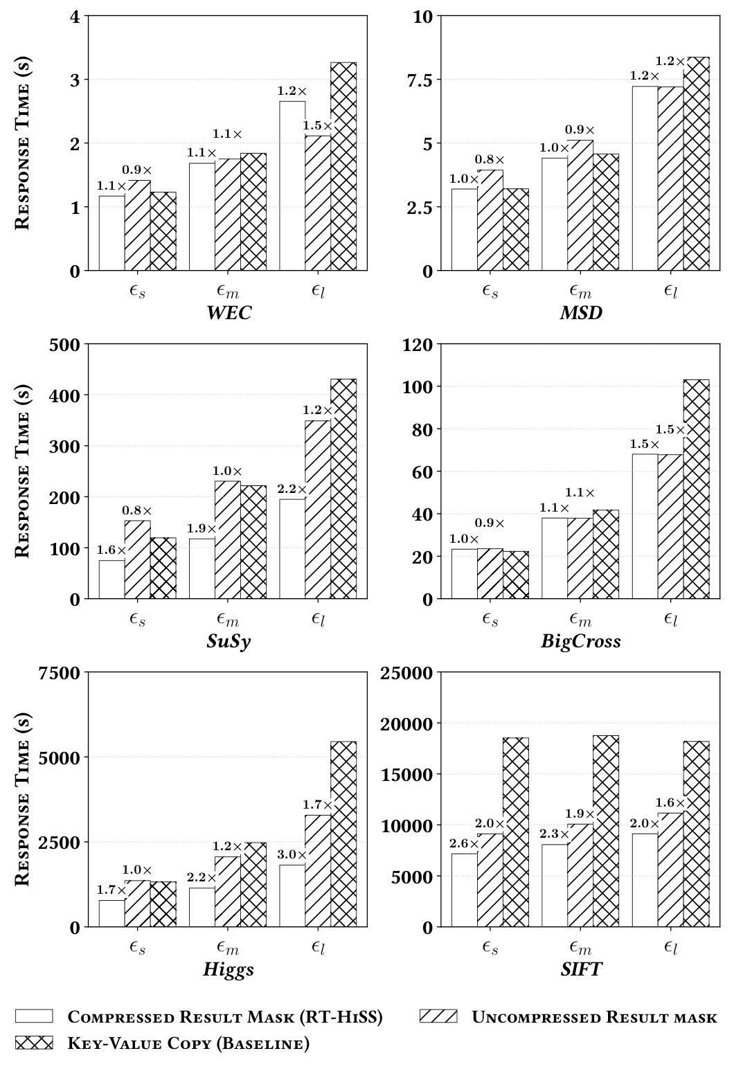
The overall performance of the algorithm is directly affected by the number of batches as each batch requires two RT kernel executions (Section IV-D). Figure 9 shows the response time of RT-HiSS compared to those in Table II. We observe that RT-HiSS outperforms key-value copy across all evaluation scenarios with an average speedup of 1.65. Similarly, except for a few evaluation scenarios, the compressed result mask copy (RT-HiSS) outperforms the uncompressed result mask copy method across all datasets and search distances with an average speedup of 1.24. This improvement is due to reduced data transfer time resulting from result mask compression.
Takeaway #2: While the representation of the result set may seem inconsequential to performance, the larger space requirements of storing key-value pairs necessitates additional batches to process all of the queries which directly corresponds to the additional overhead induced by the two-pass ray tracing approach during batching. In addition to using a result mask, compression reduces the result set size and improves data transfer time, which further improves performance.
V-H Comparison with the State-of-the-art
| Dataset | RT-HiSS | GDS-Join [6] | COSS [7] | cuVS-Brute (NVIDIA) [38] | PyTorch3D (Facebook) [37] | GTS [9] | |
| WEC | 1.16 | 1.51 (1.31) | 1.93 (1.67) | 14.88 (12.87) | 74.99 (64.87) | 3,739.45 (3,234.81) | |
| WEC | 1.67 | 3.27 (1.95) | 2.92 (1.74) | 14.88 (8.89) | 133.43 (79.71) | 5,006.74 (2,990.88) | |
| WEC | 2.71 | 7.10 (2.62) | 1.82 (0.67) | 14.88 (5.50) | 5,790.01 (2,139.69) | 5908.50 (2,183.48) | |
| MSD | 3.18 | 5.48 (1.72) | 5.00 (1.57) | 49.20 (15.46) | 544.75 (171.20) | 14,404.56 (4,526.89) | |
| MSD | 4.41 | 9.66 (2.19) | 7.38 (1.67) | 49.20 (11.17) | 1,378.92 (313.04) | 19,121.26 (4,340.81 | |
| MSD | 7.24 | 19.80 (2.74) | 15.75 (2.18) | 49.20 (6.80) | 30,243.18 (4,180.12) | 25,743.88 (3,558.24) | |
| SuSy | 74.48 | 52.14 (0.70) | 94.63 (1.27) | 9,616.54 (129.11) | 2,668.60 (35.83) | 31,704.42 (425.65 ) | |
| SuSy | 117.31 | 122.55 (1.04) | 196.50 (1.68) | 9,616.54 (81.97) | 14,846.70 (126.56) | 50,823.54 (433.24) | |
| SuSy | 195.39 | 424.32 (2.17) | 488.61 (2.50) | 9,616.54 (49.22) | TimeOut (307.08) | TimeOut (307.08) | |
| BigCross | 23.20 | 37.55 (1.62) | 94.63 (4.08) | 54,943.70 (2,368.26) | TimeOut (2,586.21) | 37,585.78 (1,620.08) | |
| BigCross | 37.87 | 143.88 (3.80) | 196.50 (5.19) | 54,943.70 (1,451.04) | TimeOut (1,584.58) | 51,911.63 (1,370.97) | |
| BigCross | 67.90 | 623.97 (9.19) | 488.61 (7.20) | 54,943.70 (809.21) | TimeOut (883.68) | TimeOut (883.68) | |
| Higgs | 775.55 | 1,801.58 (2.32) | 3,362.11 (4.34) | 46,551.90 (60.02) | 26,526.54 (34.20) | TimeOut (77.36) | |
| Higgs | 1,139.14 | 2,101.15 (1.84) | 3,292.26 (2.89) | 46,551.90 (40.87) | TimeOut (52.67) | TimeOut (52.67) | |
| Higgs | 1,81.49 | 2,819.33 (1.55) | 4,460.49 (2.45) | 46,551.90 (25.60) | TimeOut (32.99) | TimeOut (32.99) | |
| Sift | 7,169.15 | 7,732.33 (1.08 ) | TimeOut (8.37 ) | 43,250.30 (6.03 ) | TimeOut (8.37 ) | TimeOut (8.37 ) | |
| Sift | 8,070.70 | 9,232.53 (1.14 ) | TimeOut (7.43 ) | 43,250.30 (5.36 ) | TimeOut (7.43 ) | TimeOut (7.43 ) | |
| Sift | 9,134.09 | 11,290.50 (1.24 ) | TimeOut (6.57 ) | 43,250.30 (4.74 ) | TimeOut (6.57 ) | TimeOut (6.57 ) | |
| Speedup Range | [1.00, 1.00] | [0.70, 9.19] | [0.67, 8.37] | [4.74, 2,368.26] | [34.20, 4,180.12] | [425.65, 4,526.89] | |
We compare RT-HiSS with other GPU SOTA algorithms. Table IV reports the performance of RT-HiSS against the reference algorithms described in Section V-C.
Indexing Approaches: We compare to the SOTA GPU algorithms that employ an index to prune the search space. We observe that RT-HiSS outperforms GDS-Join achieving a speedup up to 9.19 across all datasets (RT-HiSS only yielded a slowdown for SuSy dataset with search distance). Similarly, RT-HiSS outperforms COSS across all datasets and distances, except for the WEC dataset with the search distance, yielding a maximum speedup of 8.37.
RT-HiSS also outperforms PyTorch3D across all datasets and search distances achieving speedup spanning 34.20 to 4,180.12 across all evaluation scenarios. Similarly, RT-HiSS outperforms GTS across all datasets and search distances. GTS reaches the timeout limit on several experiments, and is not competitive with RT-HiSS.
Brute-Force Approaches: Lastly, we compare to cuVS-Brute which is brute-force approach by NVIDIA [38]. RT-HiSS outperforms cuVS-Brute across all datasets and search distances, with minimum and maximum speedup of 4.74 and 2,368.26, respectively.
Overall, we find that RT-HiSS largely yields significant speedups as it addresses majority of the challenges of processing data-dependent workloads and scales well with dataset size. GDS-Join uses a grid-based indexing method for pruning the -neighborhood and employs an efficient batching scheme with overlapping host and GPU computation to achieve high performance. COSS uses metric-based indexing along with an efficient batching scheme. cuVS-Brute is an optimized brute-force algorithm that does not use a result estimator and allocates elements to store the result set, which limits the number of queries processed per batch and introduces batching overhead. PyTorch3D uses a maximum neighbors per query parameter to allocate memory for results, where the parameter value is set based on the selectivity level for each distance. GTS employs a pivot-based tree structure and performs poorly for large datasets and larger search distances.
Takeaway #3: The two-pass RT core approach yields two major advantages: it enables fast indexing and searching; and it enables an efficient batching scheme as it bounds the expected number of results based on the query-primitive intersections, which in turn results in saturating GPU resources. This enables significant speedups over the SOTA.
V-I Comparison with RT-based State-Of-the-art ()
| Dataset | RT-HiSS | RTNN | Speedup | |||
| Ionosphere [39] | 3 | 5,159,737 | 0.457142 | 6.22 | 8.79 | 1.41 |
| Gaia [40] | 3 | 5,000,000 | 0.374163 | 5.22 | 8.57 | 1.64 |
| Uniform | 3 | 5,000,000 | 0.023206 | 4.58 | 8.62 | 1.88 |
| Exponential | 3 | 5,000,000 | 0.001170 | 7.10 | 8.54 | 1.20 |
| Speedup Range | [1.20, 1.88] |
We compare RT-HiSS to RTNN to examine the performance on low dimensional datasets. Table V lists two real-world (Ionosphere and Gaia) and two synthetic (Uniform and Exponential) datasets used to compare the performance of RT-HiSS relative to RTNN using the search distance.44 4 We do not compare with and as RTNN does not have a batching scheme and runs out of global memory on our platform. The synthetic exponential dataset is generated using rate parameter . We observe that RT-HiSS outperforms RTNN across all datasets with speedups up to 1.88.
RT-HiSS is designed to accelerate high-dimensional distance similarity searches using RT cores; however, there are two design decisions for high-dimensional searches that reduce the performance of RT-HiSS in the low-dimensional setting as described above. Recall that RT-HiSS first identifies candidate neighbor points during the RT indexing step and later refines in a separate CUDA refinement kernel (Section IV-D). The performance of RT-HiSS for low dimensional DSS could be improved by refining within the RT kernel itself instead of using a separate kernel. Similarly, the result set compression optimization benefits high-dimensional DSS but introduces overhead for low-dimensional DSS.
V-J RT-HiSS Indexing Efficiency
Euclidean distance calculations are often the most expensive step in similarity searches due to their quadratic time complexity [10]. We compare the reduction in the number of Euclidean distance calculations performed by RT-HiSS and GDS-Join relative to cuVS-Brute using the search distance to understand the efficiency of the employed pruning method in mitigating these distance calculations. As shown in Table VI, RT-HiSS indexing using the BVH tree in 3 dimensions performs fewer distance calculations relative to GDS-Join using a grid indexing in 6 dimensions, except for the SuSy dataset where RT-HiSS is slower than GDS-Join (Table IV). This shows that RT-HiSS prunes the search space more efficiently despite indexing in only 3 dimensions. We observe a high degree of pruning for WEC, MSD, SuSy, and BigCross ( 64.7%), whereas low pruning is observed on Higgs (37.9%). Even though no pruning occurs on Sift, RT-HiSS and GDS-Join outperforms cuVS-Brute across all search distances due to locality aware computation and aborting the search early, among other optimizations.
| Dataset | RT-HiSS | GDS-Join |
| WEC | 76.4% | 74.4% |
| MSD | 71.7% | 67.9% |
| SuSy | 64.7% | 71.2% |
| BigCross | 99.2% | 99.0%) |
| Higgs | 37.9% | 0.8% |
| Sift | 0.0% | 0.0% |
V-K RT-HiSS Profiler Statistics
| Dataset | Compute Throughput | Global Memory Instructions | ||||
| RT-HiSS | Shared-None | Ratio | RT-HiSS | Shared-None | Reduction | |
| WEC | 72.75% | 28.97% | 2.51 | 1.18 G | 27.16 G | 95.66% |
| MSD | 61.00% | 26.45% | 2.31 | 7.22 G | 92.76 G | 92.22% |
| SuSy | 77.81% | 37.82% | 2.06 | 0.72 G | 37.43 G | 98.08% |
| BigCross | 60.23% | 23.66% | 2.55 | 3.41 G | 43.98 G | 92.25% |
| Higgs | 84.22% | 27.90% | 3.02 | 0.93 G | 56.38 G | 98.35% |
| Sift | 53.27% | 12.28% | 4.38 | 12.85 G | 89.49 G | 85.64% |
We profile the GPU kernel that refines candidate points to examine the impact of our proposed optimizations using Nvidia Nsight Compute. At present, RT kernels cannot be profiled using NVIDIA Nsight Compute. We compare RT-HiSS to the baseline variant that does not use shared memory tiling (Shared-None). Table VII compares the compute throughput and the number of global memory instructions for all datasets with .
We observe that compute throughput increases significantly when shared memory tiling is employed to read point data. Specifically, RT-HiSS achieves 2.06 to 4.38 compute throughout improvement compared to the baseline. Next, examining the number of global memory loads, we observe a reduction of 85.64% to 98.35% in RT-HiSS compared to the baseline. This highlights the benefit of staging data in shared memory and minimizing off-chip global memory access requests. Lastly, we find that the number of shared memory load bank conflicts spans 5.13% to 42.89% (average of 13.86%) across all datasets. These results demonstrate that the data path is well-optimized through efficient shared memory tiling and coalesced memory accesses (Section IV-C).
V-L Time Distribution Analysis

We examine the time distribution of each component of RT-HiSS. Figure 10 illustrates the fraction of total time spent in each component. The total time is averaged across all search distances (, , and ) and normalized to the range [0,1].
We observe that across all datasets, CUDA core time accounts for the majority of the total execution time (average of 59.54%) followed by the kd-tree construction time (average of 15.71%). CPU time (average of 11.30%) includes the time to identify bounding spheres of nearby points, and other host-side tasks. The FIT and two-pass RT-core approach together account for only an average of 6.58% of the total time, which is minimal compared to the other components. Thus, RT cores provide a lightweight method for efficient indexing and searching, while also enabling a batching scheme with near-perfect load balancing across batches.
VI Discussion & Conclusion
To address diverse workloads, HPC systems contain numerous processor types including tensor cores, ray tracing cores, data processing units, FPGAs, among others. We examine the design space for high-dimensional distance similarity searches and find that RT cores can be used for hardware-accelerated index searches. We address the inherent hardware limitations of RT cores with an algorithmic approach that leverages RT cores for indexing followed by CUDA cores for refinement for high-dimensional DSS, yielding significant performance gains over state-of-the-art GPU algorithms.
The paper focuses on accelerating distance similarity searches on a single-GPU system; however, our algorithm (RT-HiSS) and the proposed optimizations can be directly translated into multi-GPU systems and HPC environments with multiple nodes. In particular, after the first intersection test, RT-HiSS identifies the number of distance calculations required for each query based on the number of ray-bounding sphere intersections. This is then used to support the proposed batching scheme. In multi-GPU or HPC environments, instead of processing one batch at a time, work could be asynchronously offloaded to other GPUs or nodes while employing all the optimizations discussed in the paper. This improves scalability for large datasets and can also be exploited for near-real time distance similarity searches.
Our future work includes other types of similarity searches. Similarly to distance similarity searches, the high dimensional -nearest neighbors problem is also constrained by the inherent limitation of RT cores to three dimensions. This can be addressed by extending RT-HiSS to translate the -nearest neighbors problem into a recursive similarity search problem that expands the initial search radius () until neighbors are found. This approach yields the exact -nearest neighbors while indexing in three dimensions. All the optimizations proposed in the paper can be applied to this problem as well.
RT-HiSS is designed for large high-dimensional datasets and using it for small or low-dimensional datasets with insufficient work leads to resource underutilization including other limitations discussed in the paper, thereby resulting in degraded performance. We will examine this limitation in addition to extending RT-HiSS to support other distance similarity searches in future work.
Acknowledgment
The Chameleon testbed supported by the National Science Foundation [41] was used as part of our Artifact Description and Evaluation appendices.
References
- [1] (2017) DBSCAN Revisited, Revisited: Why and How You Should (Still) use DBSCAN. ACM Transactions on Database Systems (TODS) 42 (3), pp. 1–21. External Links: Link Cited by: §I.
- [2] (2017) A Comparative Study of Cluster Based Outlier Detection, Distance Based Outlier Detection and Density Based Outlier Detection Techniques. In 2017 International Conference on Intelligent Computing and Control Systems (ICICCS), pp. 931–935. External Links: Link Cited by: §I.
- [3] (2024) Vector Search Algorithms: A Brief Survey. In 2024 4th International Conference on Ubiquitous Computing and Intelligent Information Systems (ICUIS), pp. 365–371. External Links: Link Cited by: §I.
- [4] (2025) Blackwell GPU Architecture. Note: https://images.nvidia.com/aem-dam/Solutions/geforce/blackwell/nvidia-rtx-blackwell-gpu-architecture.pdf Cited by: §I.
- [5] (2020) Frontera: The Evolution of Leadership Computing at the National Science Foundation. In Practice and Experience in Advanced Research Computing 2020: Catch the Wave, pp. 106–111. External Links: Link Cited by: §I.
- [6] (2019) GPU-Accelerated Similarity Self-Join For Multi-Dimensional Data. In Proceedings of the 15th International Workshop on Data Management on New Hardware, pp. 1–9. External Links: Link Cited by: §I, §II-A1, §II-B1, §II-B2, §IV-A, §V-B, §V-C, TABLE IV.
- [7] (2020) A Coordinate-Oblivious Index for High-Dimensional Distance Similarity Searches on the GPU. In Proceedings of the 34th ACM International Conference on Supercomputing, pp. 1–12. External Links: Link Cited by: §I, §II-B2, §IV-A, §V-B, §V-C, TABLE IV.
- [8] (2022) RTNN: Accelerating Neighbor Search Using Hardware Ray Tracing. In Proceedings of the 27th ACM SIGPLAN Symposium on Principles and Practice of Parallel Programming, pp. 76–89. External Links: Link Cited by: §I, §I, §II-A, §II-B2, §III-A, §III, §IV-D, §V-E.
- [9] (2024) GTS: GPU-based Tree Index for Fast Similarity Search. Proceedings of the ACM on Management of Data 2 (3), pp. 1–27. External Links: Link Cited by: §I, §II-B2, §V-C, TABLE IV.
- [10] (2024) Multi-Space Tree with Incremental Construction for GPU-Accelerated Range Queries. In 2024 IEEE 31st International Conference on High Performance Computing, Data, and Analytics (HiPC), pp. 132–142. External Links: Link Cited by: §I, §I, §II-B1, §II-B2, §V-J, §V-B.
- [11] (2023) RT-kNNS unbound: Using RT Cores to Accelerate Unrestricted Neighbor Search. In Proceedings of the 37th International Conference on Supercomputing, pp. 289–300. External Links: Link Cited by: §I, §I, §II-B2, §III-A, §V-E.
- [12] (2019) Accelerating the Similarity Self-Join Using the GPU. Journal of Parallel and Distributed Computing 133, pp. 107–123. External Links: Link Cited by: §I.
- [13] (2021) Fast Radius Search Exploiting Ray-Tracing Frameworks. Journal of Computer Graphics Techniques Vol 10 (1), pp. 25–48. External Links: Link Cited by: §I, §II-A, §II-B2.
- [14] (2025) A Euclidean Distance-Based Novel Algorithm for Binary Feature Selection. Neural Processing Letters 57 (6), pp. 90. External Links: Link Cited by: §II-A.
- [15] (2024) A Review of Unsupervised Learning in Astronomy. Astronomy and Computing 48, pp. 100851. External Links: Link Cited by: §II-A.
- [16] (2010) Distance-Based Outlier Detection: Consolidation and Renewed Bearing. Proceedings of the VLDB Endowment 3 (1-2), pp. 1469–1480. External Links: Link Cited by: §II-A.
- [17] (2024) A Survey of Advancements in DBSCAN Clustering Algorithms for Big Data. In 2024 3rd International Conference on Power Electronics and IoT Applications in Renewable Energy and its Control (PARC), pp. 106–111. External Links: Link Cited by: §II-A.
- [18] (2015) Brute-Force k-Nearest Neighbors Search on the GPU. In International Conference on Similarity Search and Applications, pp. 259–270. External Links: Link Cited by: §II-A1.
- [19] (2015) Building a Balanced -d Tree in Time. Journal of Computer Graphics Techniques (JCGT) 4 (1), pp. 50–68. External Links: ISSN 2331-7418, Link Cited by: §II-B1.
- [20] (1984) R-Trees: A Dynamic Index Structure for Spatial Searching. In Proceedings of the 1984 ACM SIGMOD International Conference on Management of Data, pp. 47–57. External Links: Link Cited by: §II-B1.
- [21] (1980) Oct-Trees and Their Use in Representing Three-Dimensional Objects. Computer Graphics and Image Processing 14 (3), pp. 249–270. External Links: Link Cited by: §II-B1.
- [22] (2015) Ball*-tree: Efficient Spatial Indexing for Constrained Nearest-Neighbor Search in Metric Spaces. arXiv preprint arXiv:1511.00628. External Links: Link Cited by: §II-B1.
- [23] (1961) Adaptive Control Processes; A Guided Tour. Princeton University Press. External Links: Link Cited by: §II-B1.
- [24] (2011) 3D is Here: Point Cloud Library (PCL). In IEEE International Conference on Robotics and Automation (ICRA), Shanghai, China. External Links: Link Cited by: §II-B2.
- [25] (2026) Fixed Radius NN Search. Note: https://github.com/lxxue/FRNN Cited by: §II-B2.
- [26] (2026) Advancing RT Core-Accelerated Fixed-Radius Nearest Neighbor Search. arXiv preprint arXiv:2601.15633. External Links: Link Cited by: §II-B2.
- [27] (2026) Optix Documentation. External Links: Link Cited by: Fig. 1, Fig. 1, §III, §III.
- [28] (2024) GDBOD: Density-Based Outlier Detection Exploiting Efficient Tree Traversals on the GPU. In 2024 IEEE 31st International Conference on High Performance Computing, Data, and Analytics (HiPC), pp. 111–121. External Links: Link Cited by: §IV-A.
- [29] (2010) Optimizing Memory Access on GPUs using Morton Order Indexing. In Proceedings of the 48th annual ACM Southeast Conference, pp. 1–4. External Links: Link Cited by: §IV-C.
- [30] (2026) CUDA Toolkit Documentation. External Links: Link Cited by: §IV-D.
- [31] (2026) OWL: A Productivity Library for OptiX. Note: Available at: https://github.com/NVIDIA/OWL Cited by: §V-A.
- [32] (2014) Searching for Exotic Particles in High-Energy Physics with Deep Learning. Nature Communications 5, pp. 4308. External Links: Link Cited by: TABLE I, TABLE I.
- [33] (2018) A Detailed Comparison of Meta-Heuristic Methods for Optimising Wave Energy Converter Placements. In Proceedings of the Genetic and Evolutionary Computation Conference, pp. 1318–1325. External Links: Link Cited by: TABLE I.
- [34] (2012) StreamKM++ A Clustering Algorithm for Data Streams. Journal of Experimental Algorithmics (JEA) 17, pp. 2–1. External Links: Link Cited by: TABLE I.
- [35] (2011) The Million Song Dataset.. In Proceedings of the 12th International Conference on Music Information Retrieval (ISMIR 2011), pp. 591–596. External Links: Link Cited by: TABLE I.
- [36] (2016) SIFT10M. Note: UCI Machine Learning RepositoryDOI: https://doi.org/10.24432/C5S603 Cited by: TABLE I.
- [37] (2020) Accelerating 3D Deep Learning with PyTorch3D. arXiv:2007.08501. External Links: Link Cited by: §V-C, TABLE IV.
- [38] (2025) cuVS: GPU-Accelerated Vector Search and Clustering Library. Note: https://github.com/rapidsai/cuvsVersion 25.12.00, Apache-2.0 License Cited by: §V-C, §V-H, TABLE IV.
- [39] (2016) Exploiting Variant-Based Parallelism for Data Mining of Space Weather Phenomena. In 2016 IEEE International Parallel and Distributed Processing Symposium (IPDPS), pp. 760–769. External Links: Link Cited by: TABLE V.
- [40] (2018) Gaia Data Release 2 - Summary of the Contents and Survey Properties. Astronomy & Astrophysics 616, pp. A1. External Links: Document, Link Cited by: TABLE V.
- [41] (2020) Lessons Learned from the Chameleon Testbed. In Proceedings of the 2020 USENIX Annual Technical Conference (USENIX ATC ’20), External Links: Link Cited by: Acknowledgment.