Relative-Phase Control of Common-Bridge Survival in Collisions of Radially Excited Boson Stars
Abstract
We show that the relative phase primarily controls the survival, rather than the initial formation, of the common bridge in head-on collisions of radially excited boson stars. We vary the relative phase and track the post-contact bridge evolution across different boson-star configurations and scalar potentials. In the benchmark, all sampled phases form a common bridge, while larger phase offsets reduce its persistence; the same suppression persists across the configurations and potentials studied.
I Introduction
Boson stars are self-gravitating configurations of complex scalar fields, first constructed by Kaup and by Ruffini and Bonazzola [27, 36]. Self-interactions can substantially increase their characteristic mass scale [9]. Their equilibrium structure, stability, and dynamics have since been studied in a broad range of models; see Refs. [38, 28] for reviews. Bosonic compact objects can also form dynamically through scalar-field relaxation and gravitational cooling [39], with related formation and collapse scenarios explored for axion stars and oscillatons [23, 43, 42].
A broad range of extensions has been considered, including vector and multi-state configurations, tidal response, ultracompact solutions, and higher-dimensional models [41, 4, 7, 45, 32, 29, 31]. Ultracompact configurations have also been explored through light rings, lensing, shadows, and ray tracing [12, 25, 44, 40], while related bosonic stars have been considered in modified-gravity frameworks [14, 26, 8].
Radially excited boson stars provide a direct setting in which to study internal scalar-field structure. Their profiles contain radial nodes, and their stability differs from that of fundamental configurations. Early nonlinear evolutions found excited states to be dynamically fragile [3]. Self-interactions can extend their lifetime in spherical dynamics [37, 5], while multidimensional evolutions reveal additional instability channels and nonlinear morphologies [6]. Recent work has further examined their radial spectra and dynamical signatures [21]. Collisions of excited configurations can produce transient chain- and ring-like structures [6, 20].
Binary dynamics introduces another internal parameter: the relative phase of the complex scalar fields. Early head-on simulations showed that otherwise identical boson stars with different phases can follow different merger dynamics and radiate differently [35]. Phase dependence also appears in orbital binaries [34]. More recent work has examined scalar-soliton collisions [22], boson-star inspirals and merger signals [16, 17, 15], head-on merger studies [18, 19], relativistic scattering [13], and mixed black-hole–boson-star systems [30, 33]. For the chain-forming channel considered here, it remains unclear whether the relative phase acts mainly on the formation of the common structure or on its subsequent survival.
For radially excited boson stars, our previous work identified a separate control on chain formation [20]. Visible chain-like transients appeared only when the binary collision occurred at a stage compatible with the breathing dynamics of the corresponding isolated star. Varying the initial separation shifted the collision relative to the same internal clock and produced the corresponding turn-on and turn-off of the chain. Collision timing therefore selects whether the chain-forming channel is accessible.
The remaining question is what controls the common bridge once it has formed. Figure 1 shows the same evolution through the energy density and the scalar-field magnitude. The former emphasizes the density morphology, while the latter makes the developing bridge more apparent. The central region first fills as the stars approach, develops a finite-amplitude common bridge, and can later lose that connectivity. The maximum chain score identifies the most pronounced instantaneous morphology, but does not determine how long the bridge survives.


We study this question by varying the relative phase in equal-mass head-on collisions of radially excited boson stars. In the benchmark configuration, all five sampled phases reach both the common- and strong-bridge levels. Once the evolutions are aligned at first contact, their early bridge growth is similar; the phase dependence becomes clear only later in the post-contact evolution. Over the interval , the anti-phase case retains about of the accumulated bridge connectivity of the in-phase case.
The same phase-ordered suppression persists when the central scalar amplitude and quartic self-interaction strength are varied, and is also present for solitonic boson stars. Relative phase therefore acts primarily on the survival of an already formed common bridge rather than on its initial formation. We interpret this behaviour through the spatial phase variation required to connect finite-amplitude scalar configurations with a nonzero phase mismatch. Together with the timing-window mechanism of Ref. [20], this separates two controls on the dynamics: collision timing determines whether the chain-forming channel is reached, while relative phase controls how persistent the common bridge is once it forms.
Throughout this work, we employ geometric units with and set the scalar-field mass to .
II Model, numerical setup, and bridge diagnostics
II.1 Boson-star models
We consider a complex scalar field minimally coupled to gravity, with action
| (1) |
Our main simulations use the quartically self-interacting massive model,
| (2) |
while the robustness analysis also includes solitonic boson stars with
| (3) |
Equilibrium boson stars are constructed with the harmonic ansatz
| (4) |
where is the field frequency and is the central scalar-field amplitude. Throughout this work we consider the radially excited branch, where denotes the number of radial nodes. The boson-star construction and numerical framework follow our previous work [18, 19, 20].
II.2 Binary setup
The numerical evolutions use the same GRChombo-based modified-Cartoon framework [2], AMR hierarchy, and resolution as in Refs. [18, 19, 20], with the modified-Cartoon implementation following Refs. [11, 10, 1]. Binary initial data are constructed from two equal-mass, nonspinning boson stars using the improved superposition prescription of Refs. [22, 24, 16]. The stars are initially separated by and undergo a head-on collision. Unless stated otherwise, each star is given an inward velocity . Our benchmark configuration is
| (5) |
To introduce a relative phase, we denote the scalar field and momentum variable of the two individual stars entering the superposition by and , respectively. Taking star as the phase reference, we apply a global rotation to star ,
| (6) |
For the equal-mass head-on configurations considered here, and are related by interchange of the two stars, so it is sufficient to restrict the scan to . Thus we sample five relative phases,
| (7) |
All other initial parameters are held fixed within each phase scan.
II.3 Common-bridge diagnostics
We characterize the connectivity between the two stars using the bridge ratio , introduced in Ref. [20]. It compares the near-axis density weight in the central region with the weaker of the two stellar-side density peaks. Denoting these quantities by , , and , respectively, we write
| (8) |
Thus corresponds to two well-separated density concentrations, while increasing indicates progressive filling of the region between them. The detailed construction of , , and is given in Appendix A.
For the timing analysis we use three reference levels,
| (9) |
The corresponding event times are denoted by , , and . The three levels provide operational markers for weak initial contact, common-bridge formation, and strong-bridge formation, respectively. Once a strong bridge has formed, denotes its first sustained return below . The precise sustainment criteria are given in Appendix A.
To separate differences in collision timing from the subsequent bridge evolution, we define the contact-aligned time
| (10) |
Hereafter, denotes the same bridge ratio expressed in this shifted time coordinate. We quantify the accumulated bridge connectivity over an interval by
| (11) |
For comparisons between different equilibrium configurations, we also use the response normalized to the corresponding in-phase evolution,
| (12) |
We retain the chain score of Ref. [20] as an auxiliary morphology diagnostic and define . The corresponding time identifies the most pronounced chain-like configuration. We do not use or the number of chain episodes as the primary measure of bridge survival: these characterize instantaneous morphology, whereas provides a continuous measure of the accumulated bridge connectivity over a specified time interval.
III Relative phase and the survival of the common bridge
We first vary only the relative phase in the benchmark configuration of Eq. (5). Figure 2 summarizes the characteristic times for the five phase offsets. Increasing produces a modest but systematic delay: shifts from at to at , while shifts from to . All five cases nevertheless reach both the common- and strong-bridge thresholds. The relative phase therefore does not prevent the initial formation of a common bridge in this configuration.

The later evolution is more strongly phase dependent. Figure 3 (left) shows the bridge ratio directly. The low-phase cases develop a stronger and more persistent central connection, whereas the large-phase cases reach lower bridge ratios and weaken earlier. Sustained breakup occurs for , , and , while the low-phase cases remain strongly connected over the interval shown. The main phase dependence is therefore associated with the persistence of the bridge rather than with its initial formation.
This distinction becomes clearer after removing the phase-dependent shift in the contact time. Figure 3 (right) shows the same evolutions in the contact-aligned coordinate . During the first time units after contact, the five bridge ratios remain close, showing comparable initial bridge build-up. A clear separation develops only later, beginning around –. The low-phase systems remain strongly connected, whereas the large-phase systems turn over and progressively lose connectivity.


Motivated by this separation, we use
| (13) |
as a common post-contact window for the quantitative comparisons below. This interval lies after the initial bridge build-up and covers the stage where the phase-dependent loss of connectivity is pronounced. For the benchmark configuration, direct integration of gives
| (14) |
Normalizing to the in-phase evolution yields
| (15) |
Thus the anti-phase case retains about of the accumulated post-contact bridge connectivity of the in-phase case over the same interval.
The benchmark therefore points to a simple interpretation: relative phase primarily controls the post-contact survival of the common bridge, rather than its initial formation. In the next section we test whether this behaviour persists when the equilibrium configuration and scalar potential are changed.
IV Robustness of the phase response
We next test whether the phase response found in the benchmark persists away from the fiducial configuration. The same five relative phases are used throughout, with evaluated over the bridge-survival window .
IV.1 Central-amplitude dependence
We first keep and fixed and compare with the benchmark value . Figure 4 shows and its normalized counterpart . The benchmark has a larger throughout the phase scan, but both amplitudes show the same overall phase ordering.
At , for and for . For both configurations shown here, decreases monotonically across the sampled phases, although the strength of the response depends on .


IV.2 Quartic self-interaction
We next fix and , and compare with the benchmark value . The configuration has a larger throughout the phase scan, while the normalized curves in Fig. 5 are nearly coincident.
At , for and for . The anti-phase evolution therefore retains about of the corresponding in-phase accumulated connectivity in both cases. The normalized phase response is nearly unchanged under this factor-of-two variation in , despite the change in the absolute scale of .

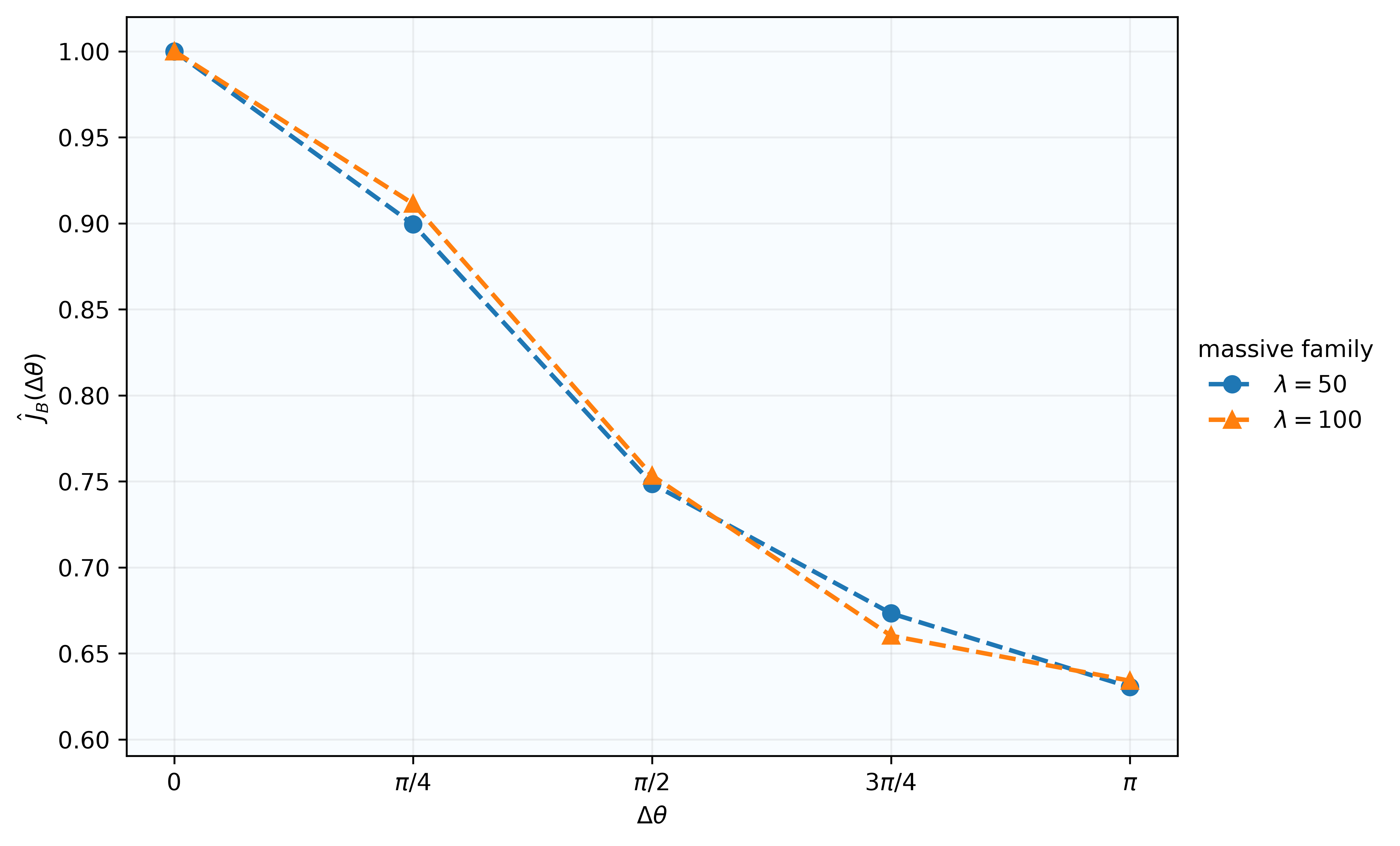
IV.3 Solitonic boson stars
We finally change the scalar potential itself. For the solitonic model of Eq. (3), we take and , keeping and . The results are shown in Fig. 6.
The unnormalized again depends on the equilibrium configuration, whereas the normalized curves remain close over the full phase range. At , the two configurations retain about – of their corresponding in-phase accumulated connectivity. Both solitonic scans decrease monotonically across the five sampled phases.


Across these scans, the absolute scale of remains configuration dependent. For all configurations shown here, however, decreases monotonically across the five sampled phases. The benchmark suppression is therefore not tied to a single central amplitude, quartic coupling, or scalar potential.
V Physical interpretation
The contact-aligned results constrain the interpretation of the phase dependence. Increasing produces a modest delay in the collision, but this delay alone cannot explain the subsequent bridge hierarchy. After alignment at , the five bridge ratios remain close for roughly the first time units and begin to separate only around –; see Fig. 3. The main dynamical effect of the relative phase therefore emerges during the post-contact evolution.
At the level of the initial overlap, the superposed field contains the phase-dependent term
| (16) |
The relative phase can therefore enhance or suppress the local field magnitude in the overlap region. The evolutions show, however, that this does not prevent the initial bridge from forming: all five benchmark phases reach both the common- and strong-bridge thresholds.
The subsequent evolution suggests a phase-gradient interpretation. Extending the notation of Eq. (4), we write the evolving field locally as , where is the local phase. Its spatial-gradient contribution is
| (17) |
where denotes the spatial gradient. For the in-phase case, no phase mismatch is imposed between the two sides by the initial data. At nonzero , a finite-amplitude connection must accommodate the mismatch through a spatial phase variation. The corresponding contribution is weighted by , and can therefore be reduced if the field amplitude decreases where the phase changes rapidly. A large phase offset thus disfavors a broad, persistent high-amplitude connection.
The amplitude scan provides a useful consistency check of this picture. At , the normalized response is for , compared with for the benchmark ; see Fig. 4. The lower-amplitude configuration is therefore less sensitive to the phase offset, consistent with the weighting in Eq. (17). Since changing also changes the underlying equilibrium star, this comparison supports rather than directly tests the phase-gradient interpretation.
The same picture is consistent with the robustness under changes of the scalar potential. The massive and solitonic models have different radial self-interactions, but both are -symmetric and share the same canonical phase-gradient structure. Their absolute bridge responses differ, while the suppression with increasing persists; see Figs. 5 and 6.
This interpretation is complementary to the timing-window mechanism of Ref. [20]. There the collision time controls whether the binary encounters a stage compatible with visible-chain formation. Here all five benchmark phases form a strong bridge, while the survival hierarchy remains after aligning the evolutions at . Relative phase therefore acts primarily on the persistence of an already formed common bridge. We do not separately measure the bridge-region phase-gradient contribution here, so Eq. (17) provides a physical interpretation rather than a direct diagnostic.
VI Conclusion
We have studied how relative phase affects the common bridge in head-on collisions of radially excited boson stars. In the benchmark configuration, all five sampled phases reach both the common- and strong-bridge thresholds. After aligning the evolutions at first contact, the bridge ratios remain close during the early post-contact stage and separate only later. Relative phase therefore affects primarily the survival of the common bridge rather than its initial formation.
Over the post-contact interval , the anti-phase benchmark retains about of the accumulated bridge connectivity of the in-phase case. The absolute response depends on the equilibrium configuration, but the phase-ordered suppression persists across the sampled central amplitudes, quartic couplings, and solitonic models.
The results are consistent with a phase-gradient interpretation. A finite-amplitude connection between regions with different phases must accommodate the mismatch through spatial phase variation, whose gradient contribution is weighted by . Large phase offsets therefore disfavor a broad, persistent high-amplitude connection. The phase-gradient argument is therefore an interpretation of the observed survival hierarchy rather than a direct diagnostic.
Together with the timing-window mechanism identified in our previous work, these results distinguish the conditions for chain formation from the subsequent survival of the common bridge. Collision timing determines whether the encounter occurs at a stage compatible with chain formation, whereas relative phase controls the persistence of the common bridge once it has formed.
Acknowledgements.
The author acknowledges HIAS for access to the “Quantum Universe Physical Simulation Platform”. This work was supported by the National Natural Science Foundation of China under Grant No. 12505066.Appendix A Bridge-diagnostic construction
The bridge diagnostic is constructed from the energy density in the axisymmetric sampling region. Let denote the centre of the -th sampling interval along the collision axis, with spacing . We define the near-axis density weight
| (18) |
where is the energy density and is the determinant of the spatial metric. The factor accounts for the axisymmetric volume element. In practice, Eq. (18) is evaluated as a discrete sum over the diagnostic grid.
The transverse extent of the near-axis region is chosen as
| (19) |
where is the radius of the diagnostic sampling region. For all runs considered in the main text we use
| (20) |
which gives
| (21) |
Restricting the transverse integration to this near-axis region suppresses contributions from off-axis material and makes the diagnostic sensitive to the filling of the region between the two stars.
Let be the midpoint of the initial binary and the sampling interval closest to it. The central bridge weight is obtained by averaging over seven neighbouring axial intervals,
| (22) |
This averaging prevents a single sampling interval from dominating the bridge estimate.
The left- and right-side peaks are extracted from the same near-axis profile, excluding the central bridge region,
| (23) |
The bridge ratio used throughout the main text is then
| (24) |
Normalizing by the weaker stellar-side peak reduces sensitivity to small left–right asymmetries. For two separated configurations the central region is depleted and ; increases as this region becomes filled during the collision.
We use the three reference levels
| (25) |
For each level , the corresponding event time is assigned to the first output of the earliest sequence of three consecutive diagnostic outputs satisfying
| (26) |
The sustainment condition removes isolated threshold crossings caused by short-time fluctuations.
After the strong-bridge level has been reached, bridge breakup is defined by the first downward crossing of for which
| (27) |
holds for three consecutive diagnostic outputs. We require an actual downward crossing, with the preceding output satisfying . Once the sustainment condition is met, is assigned to the crossing obtained by linear interpolation between the two outputs bracketing the crossing.
Appendix B Constraint monitoring and convergence tests
We monitor the Hamiltonian and momentum constraints throughout the benchmark phase scan. Figure 7 shows their norms for the five relative phases. Following the initial transient, the Hamiltonian and momentum norms remain at roughly and , respectively, until the strongly nonlinear late-time evolution. Their subsequent growth occurs at approximately the same stage for all five phases, reaching for the Hamiltonian constraint and for the momentum constraint before decreasing again.
The bridge-survival interval used in the main analysis, , ends at – for the benchmark runs and therefore precedes the sharp late-time increase of both constraint norms.


We repeated the full benchmark phase scan at three base-grid resolutions,
where denotes the number of grid points on the coarsest AMR level covering the full computational domain. The domain length is , and the same AMR setup is used throughout. The production runs use .
The diagnostic output cadence changes with resolution. For this comparison we therefore determine the , , and crossings directly from the raw data by linear interpolation. For breakup we use the first interpolated downward crossing of after the strong-bridge level has been reached. These interpolated times are used only for the resolution comparison; the event times quoted in the main text retain the sustainment criteria of Appendix A. This avoids mixing spatial-resolution effects with the different physical duration represented by three consecutive diagnostic outputs.
Table 1 lists the characteristic times for all five phases.
| 128 | 209.669 | 226.096 | 232.229 | — | |
|---|---|---|---|---|---|
| 256 | 209.686 | 226.100 | 232.211 | — | |
| 512 | 209.691 | 226.103 | 232.218 | — | |
| 128 | 210.330 | 226.778 | 232.731 | — | |
| 256 | 210.348 | 226.790 | 232.671 | — | |
| 512 | 210.351 | 226.797 | 232.593 | — | |
| 128 | 211.817 | 227.897 | 236.343 | 268.492 | |
| 256 | 211.804 | 227.907 | 236.378 | 268.410 | |
| 512 | 211.665 | 227.893 | 236.382 | 268.400 | |
| 128 | 214.782 | 231.419 | 238.117 | 263.733 | |
| 256 | 214.811 | 231.463 | 237.401 | 263.693 | |
| 512 | 214.819 | 231.462 | 237.401 | 263.678 | |
| 128 | 215.067 | 231.864 | 238.751 | 263.752 | |
| 256 | 215.065 | 231.871 | 238.698 | 263.752 | |
| 512 | 215.065 | 231.874 | 238.565 | 263.751 |
The characteristic times are stable across the three resolutions. The phase ordering of the three upward crossings, as well as the presence or absence of bridge breakup, is unchanged. Between the production and highest resolutions, and , the largest shifts over the full phase scan are , , and for the , , and crossings, respectively. For the three phases that undergo bridge breakup, the largest change in is .
The resolution study therefore leaves the characteristic bridge times, the ordering of the upward crossings, and the breakup classification unchanged. Since these are derived threshold-crossing times in an AMR evolution, we do not assign a formal Richardson convergence order to them.
References
- [1] (2001) Symmetry without symmetry: Numerical simulation of axisymmetric systems using Cartesian grids. Int. J. Mod. Phys. D 10, pp. 273–290. External Links: gr-qc/9908012, Document Cited by: §II.2.
- [2] (2021) GRChombo: An adaptable numerical relativity code for fundamental physics. J. Open Source Softw. 6 (68), pp. 3703. External Links: 2201.03458, Document Cited by: §II.2.
- [3] (1998) Dynamical Evolution of Boson Stars II: Excited States and Self-Interacting Fields. Phys. Rev. D 58, pp. 104004. External Links: gr-qc/9712064, Document Cited by: §I.
- [4] (2010) Multi-state Boson Stars. Phys. Rev. D 81, pp. 044031. External Links: 0908.2435, Document Cited by: §I.
- [5] (2023) Stability and physical properties of spherical excited scalar boson stars. Phys. Rev. D 107 (8), pp. 084022. External Links: 2302.08900, Document Cited by: §I.
- [6] (2026) Stability and collisions of excited spherical boson stars: Glimpses of chains and rings. Phys. Rev. D 113 (2). External Links: 2506.06442, Document Cited by: §I.
- [7] (2017) Testing strong-field gravity with tidal Love numbers. Phys. Rev. D 95 (8), pp. 084014. External Links: 1701.01116, Document Cited by: §I.
- [8] (2025) Proca stars and their frozen states in an infinite tower of higher-derivative gravity. External Links: 2512.24584 Cited by: §I.
- [9] (1986) Boson Stars: Gravitational Equilibria of Self-Interacting Scalar Fields. Phys. Rev. Lett. 57, pp. 2485–2488. External Links: Document Cited by: §I.
- [10] (2016) Dimensional reduction in numerical relativity: Modified cartoon formalism and regularization. Int. J. Mod. Phys. D 25 (09), pp. 1641013. External Links: 1603.00362, Document Cited by: §II.2.
- [11] (2017) Extraction of gravitational-wave energy in higher dimensional numerical relativity using the Weyl tensor. Class. Quant. Grav. 34 (3), pp. 035010. External Links: 1609.01292, Document Cited by: §II.2.
- [12] (2017) Lensing and dynamics of ultra-compact bosonic stars. Phys. Rev. D 96 (10), pp. 104040. External Links: 1709.06118, Document Cited by: §I.
- [13] (2026) Gravitational Scattering of Solitonic Boson Stars: Analytics vs Numerics. Phys. Rev. Lett. 137 (2), pp. 021401. External Links: 2512.00945, Document Cited by: §I.
- [14] (2023) Boson stars in massless and massive scalar-tensor gravity. Phys. Rev. D 108 (10), pp. 104064. External Links: 2310.05200, Document Cited by: §I.
- [15] (2026) Lessons from binary dynamics of inspiralling equal-mass boson-star mergers. External Links: 2604.25582 Cited by: §I.
- [16] (2023) Unequal-mass boson-star binaries: initial data and merger dynamics. Class. Quant. Grav. 40 (8), pp. 085009. External Links: 2212.08023, Document Cited by: §I, §II.2.
- [17] (2024) Gravitational-Wave Data Analysis with High-Precision Numerical Relativity Simulations of Boson Star Mergers. Phys. Rev. Lett. 133 (13), pp. 131401. External Links: 2406.02715, Document Cited by: §I.
- [18] (2024) Gravitational Waves in Boson Star Mergers. Ph.D. Thesis, King’s Coll. London, King’s College London. Cited by: §I, §II.1, §II.2.
- [19] (2026) Massive boson stars: Stability and GW emission in head-on mergers. Phys. Rev. D 113 (10), pp. 104065. External Links: 2512.15242, Document Cited by: §I, §II.1, §II.2.
- [20] (2026) Timing-Window Mechanism for Chain-Like Transients in Collisions of Radially Excited Boson Stars. External Links: 2605.19572 Cited by: §I, §I, §I, §II.1, §II.2, §II.3, §II.3, §V.
- [21] (2026) Radial spectra and dynamical signatures of excited boson stars. External Links: 2608.06067 Cited by: §I.
- [22] (2019) Gravitational Wave Emission from Collisions of Compact Scalar Solitons. Phys. Rev. D 99 (4), pp. 044046. External Links: 1802.06733, Document Cited by: §I, §II.2.
- [23] (2017) Black hole formation from axion stars. JCAP 03, pp. 055. External Links: 1609.04724, Document Cited by: §I.
- [24] (2022) Malaise and remedy of binary boson-star initial data. Class. Quant. Grav. 39 (7), pp. 074001. External Links: 2108.11995, Document Cited by: §II.2.
- [25] (2025) Orbits of photon in Bardeen-boson stars and their frozen states. External Links: 2503.14984 Cited by: §I.
- [26] (2026) Boson Stars in Teleparallel Gravity with a Nonminimally Coupled Field: The Violation of Energy Conditions and Gravitational Waveforms from EMRIs. External Links: 2607.02017 Cited by: §I.
- [27] (1968) Klein-Gordon Geon. Phys. Rev. 172, pp. 1331–1342. External Links: Document Cited by: §I.
- [28] (2023) Dynamical Boson Stars. Living Rev. Rel. 26 (1), pp. 1. External Links: 1202.5809, Document Cited by: §I.
- [29] (2025) Long-Term Stable Nonlinear Evolutions of Ultracompact Black-Hole Mimickers. Phys. Rev. Lett. 135 (13), pp. 131402. External Links: 2504.17775, Document Cited by: §I.
- [30] (2026) Black Hole-Boson Star Binaries: Gravitational Wave Signals and Tidal Disruption. External Links: 2604.06312 Cited by: §I.
- [31] (2026) Boson stars in dimensions: stability, oscillation frequencies, and dynamical evolutions. Class. Quant. Grav. 43 (8), pp. 085014. External Links: 2510.13988, Document Cited by: §I.
- [32] (2026) Perturbations of Solitonic Boson Stars: Nonlinear Radial Stability and Binding Energy. J. Phys. Conf. Ser. 3177 (1), pp. 012047. External Links: 2508.11757, Document Cited by: §I.
- [33] (2026) Boson star-black hole binaries: initial data and head-on collisions. External Links: 2604.15240 Cited by: §I.
- [34] (2008) Orbital Dynamics of Binary Boson Star Systems. Phys. Rev. D 77, pp. 044036. External Links: 0706.2435, Document Cited by: §I.
- [35] (2007) Head-on collisions of boson stars. Phys. Rev. D 75 (6), pp. 064005. External Links: gr-qc/0612067, Document Cited by: §I.
- [36] (1969) Systems of Self-Gravitating Particles in General Relativity and the Concept of an Equation of State. Phys. Rev. 187, pp. 1767–1783. External Links: Document Cited by: §I.
- [37] (2022) Self-interactions can stabilize excited boson stars. Class. Quant. Grav.. External Links: 2110.03000, Document Cited by: §I.
- [38] (2003) General Relativistic Boson Stars. Class. Quant. Grav. 20, pp. R301–R356. External Links: Document Cited by: §I.
- [39] (1994) Formation of Solitonic Stars Through Gravitational Cooling. Phys. Rev. Lett. 72, pp. 2516–2519. External Links: gr-qc/9309015, Document Cited by: §I.
- [40] (2026) Ray tracing ultracompact boson stars: visibility modulations and incomplete photon rings. External Links: 2606.30729 Cited by: §I.
- [41] (2024) General relativistic polarized Proca stars. Phys. Rev. D 109 (2), pp. 024019. External Links: 2309.04345, Document Cited by: §I.
- [42] (2020) Black hole formation in relativistic Oscillaton collisions. JCAP 01, pp. 027. External Links: 1910.01950, Document Cited by: §I.
- [43] (2018) Formation of Relativistic Axion Stars. JCAP 10, pp. 005. External Links: 1806.09367, Document Cited by: §I.
- [44] (2025) Emerging black hole shadow from collapsing boson star. External Links: 2503.14159 Cited by: §I.
- [45] (2026) Tidal Love numbers of multi-state Boson stars. External Links: 2607.27587 Cited by: §I.