Does the Power-Law Advantage in the Tails Outweigh the Global q-Gaussian Description?
Abstract
Financial markets are complex systems whose return distributions exhibit heavy tails, traditionally described by power laws. An alternative framework based on Tsallis nonextensive statistical mechanics allows both the central region and the tails of the distribution to be represented by a single q-Gaussian functional form. In this work, we systematically compare these two descriptions across different time scales, considering stock markets from Brazil and the United States, as well as traditional assets and cryptocurrencies. The q-Gaussian parameters are estimated using the method of moments ratio, whereas the power-law parameters are obtained by maximum likelihood estimation in the asymptotic region. The quality of the fits is assessed using goodness-of-fit measures, bootstrap resampling, and the Vuong test. When the analysis is restricted exclusively to the extreme tails, the power law generally provides a better description, as expected from the asymptotic power-law behavior of the q-Gaussian itself. However, this superiority is not sufficiently pronounced to outweigh the main advantage of the q-Gaussian: its ability to provide a consistent description of the entire distribution, including the central peak, bulk, and tails, over all investigated time scales. Moreover, the evolution of the parameter offers a simple and direct characterization of aggregational Gaussianity and of the transition between heavy- and short-tailed statistical regimes, without requiring separate fits for different regions of the distribution. These results indicate that, although the power law remains particularly suitable for describing extreme events, the q-Gaussian provides a broader and more practical framework for characterizing the statistical evolution of financial returns.
Keywords:
Econophysics , Tsallis statistics , Critical phenomena in economic markets , Stylized facts , Aggregational Gaussianity1 Introduction
The analysis of complex time series, ranging from fluid turbulence to the high-frequency dynamics of financial markets, has repeatedly revealed statistical properties that cannot be adequately described within the framework of conventional Gaussian statistics. In econophysics, financial returns are known to display a number of robust empirical regularities, commonly referred to as stylized facts, among which heavy-tailed distributions and aggregational Gaussianity are particularly prominent [1, 2, 3, 4, 5, 6]. At short aggregation intervals, , return distributions exhibit pronounced deviations from Gaussian behavior, with a substantially enhanced probability of extreme fluctuations. As increases, however, the distributions progressively approach a Gaussian form. This scale-dependent evolution constitutes one of the most characteristic statistical signatures of financial time series.
Heavy tails are traditionally associated with power-law behavior and have consequently been extensively analyzed within this framework. Nevertheless, identifying a genuine power law in empirical data is a subtle statistical problem, since power-law behavior is expected only beyond a sufficiently large threshold and its detection may depend strongly on the definition of the asymptotic region, the estimation procedure, and the finite amount of data available [7, 8, 9, 10]. Moreover, a pure power law is intrinsically a description of the tail and therefore does not provide a unified representation of the central region and the extreme fluctuations of the return distribution.
An alternative description arises naturally from the nonextensive statistical-mechanics formalism introduced by Tsallis [11, 12]. Within this framework, the Gaussian distribution is generalized to the -Gaussian, characterized by the entropic index . For , the -Gaussian exhibits heavy tails, whereas the standard Gaussian distribution is continuously recovered in the limit . Importantly, the -Gaussian provides a single functional form capable of describing the central peak, the intermediate region, and the tails of the distribution. In this sense, it offers a particularly appealing framework for financial returns, for which both the bulk of ordinary fluctuations and the occurrence of extreme events are relevant [13, 14, 15].
The connection between these two descriptions is especially important. For sufficiently large fluctuations, the -Gaussian itself asymptotically approaches a power law. Therefore, if the statistical analysis is restricted exclusively to the far-tail region, one may naturally expect a pure power-law fit, whose parameters are optimized specifically for that region, to perform at least as well as, and possibly better than, a -Gaussian whose parameters characterize the distribution more globally. Consequently, the relevant question is not simply whether a power law can provide a better fit to the most extreme observations, but whether such an improvement is sufficiently significant to justify abandoning a distribution that simultaneously describes the central peak, the bulk, and the tails.
This distinction becomes particularly relevant when different temporal aggregation scales are considered. Aggregational Gaussianity implies a progressive transformation of the return distribution from a heavy-tailed form at short time scales toward Gaussian statistics at longer scales. Within the nonextensive framework, this evolution can be monitored directly through the parameter : strongly non-Gaussian distributions are associated with , while the relaxation toward provides a simple quantitative representation of the approach to the Gaussian regime [6, 12, 16]. Thus, rather than fitting different functional forms independently to different portions of the distribution or at different aggregation scales, the evolution of a single parameter can be used to characterize the transition between heavy- and short-tailed statistical regimes.
This perspective suggests that the comparison between the -Gaussian and the pure power law should be performed at two complementary levels. On the one hand, the extreme-tail region must be analyzed separately in order to determine whether a genuine power-law description provides a statistically superior representation of rare events. On the other hand, the complete distribution must also be considered, since financial dynamics cannot be characterized exclusively by its most extreme fluctuations. A statistically meaningful comparison must therefore distinguish between local superiority in the asymptotic tail and the ability to provide a robust description of the distribution as a whole across different time scales.
In this work, we address precisely this issue by systematically comparing the -Gaussian and pure power-law descriptions of financial returns over a broad range of temporal aggregation scales. Our analysis encompasses conventional stock markets from both Brazil and the United States, as well as cryptocurrencies, allowing us to test the robustness of these statistical descriptions across different markets and classes of financial assets. We examine not only the quality of the global description provided by the -Gaussian, but also the relative performance of the two distributions when the comparison is restricted to the asymptotic tail. This allows us to investigate whether the expected advantage of the power law in the extreme region is sufficiently pronounced to outweigh the broader statistical information retained by the -Gaussian, while simultaneously using the evolution of to characterize aggregational Gaussianity and the relaxation between distinct statistical regimes.
The remainder of this paper is organized as follows. In Section 2, we describe the data employed in this study. Section 3 presents the methodology used to estimate, evaluate, and compare the different statistical fits. The results are presented and discussed in Section 4. Finally, Section 5 summarizes the main findings and presents our conclusions.
2 Data Description
In this study, we analyze financial data from three distinct groups: U.S. stocks traded on the New York Stock Exchange (NYSE) and NASDAQ, Brazilian stocks traded on BOVESPA, and cryptocurrencies. The U.S. stock data span 23 years, from 2003 to 2025; the Brazilian stock data cover the period from 2020 to 2025; and the cryptocurrency data extend over approximately seven years, from 2017 to 2025.
The assets included in each group were selected to provide a heterogeneous and representative sample. For the traditional equity markets, both in the United States and Brazil, we considered companies from a broad range of economic sectors, including technology, finance, health care, energy, consumer goods, and industry. The cryptocurrency sample was likewise chosen to reflect different technological and functional profiles, encompassing established stores of value, smart-contract platforms, privacy-oriented currencies, and networks designed for cross-border payments and remittances. This diversified selection allows us to assess whether the statistical properties investigated in this work persist across different markets, asset classes, sectors, and underlying economic or technological structures.
2.1 Data Collection
The data used in this study were obtained through the MetaTrader 5 trading platform, using the market data feed provided by XP Investimentos 11 1 https://www.xpi.com.br/. The entire data-acquisition procedure was automated in Python through the platform’s official integration library. The resulting financial time series have an intraday resolution of one minute, allowing us to exploit the longest historical records available on the broker’s server for each market. For the U.S. market, the dataset spans from 2003 to the end of 2025. For the Brazilian market, owing to limitations in the server-side storage of high-frequency historical data, the available period extends from late 2020 to the end of 2025.
Cryptocurrency data were obtained from Binance Data Vision 22 2 https://data.binance.vision/ , the official public data repository maintained by the Binance exchange. The acquisition procedure was likewise fully automated in Python, using programmed requests to retrieve the data directly from the repository. As for the traditional financial markets, cryptocurrency prices were sampled at a one-minute intraday resolution. The corresponding dataset spans from 2017 to the end of 2025.
3 Methodology for analysis
3.1 Returns
One of the fundamental concepts underlying this study is the financial return. It represents the relative price difference over a given time window. One could define this quantity as:
where denotes the asset price. However, many important properties can be lost with this linear approach, such as time additivity and numerical symmetry. To address this issue, the most widely used definition for financial returns is the log-return:
| (1) |
3.2 Power-Laws
A fundamental aspect in the statistical characterization of financial markets is the analysis of return distributions. One of their most robust empirical properties is the occurrence of heavy tails, indicating that extreme price fluctuations occur considerably more frequently than would be expected under a Gaussian description [4, 17, 18]. A commonly adopted representation for such tails is the pure power law in ,
| (2) |
where is the tail exponent and defines the lower bound above which the power-law behavior is assumed to hold. Power-law tails have been reported for several financial markets and over a broad range of temporal scales [1, 2, 3, 7, 8]. In particular, seminal studies of U.S. financial data found that the tails of return distributions for market indices and individual stocks could be described, over substantial ranges, by approximately inverse-cubic power laws [17, 18]. Similar scale-free behavior has motivated the widespread use of power laws in the characterization of large financial fluctuations and extreme events [19].
Nevertheless, such a description is not expected to remain valid at all aggregation scales. At relatively short time intervals, , return distributions are strongly leptokurtic and heavy-tailed, whereas increasing generally produces a progressive convergence toward a Gaussian distribution. This phenomenon, usually referred to as aggregational Gaussianity, is one of the best-known stylized facts of financial returns [4, 20]. Consequently, the range over which a pure power law provides an adequate representation is intrinsically scale dependent and may differ substantially among markets and asset classes.
An additional limitation is that a pure power law is intrinsically a model for the asymptotic tail rather than for the complete return distribution. Consequently, it does not retain information about the central peak and the bulk of the distribution, which contain the majority of the observations. Only data satisfying contribute directly to the fitting procedure, making the determination of a central statistical issue.
The choice of this threshold cannot, in general, be made arbitrarily. Different values of may lead to different estimates of the exponent , particularly when the available tail contains only a limited number of observations. Clauset, Shalizi, and Newman [9] emphasized this difficulty and proposed a systematic framework based on maximum-likelihood estimation, Kolmogorov–Smirnov statistics, and likelihood-ratio comparisons for identifying and testing power-law behavior in empirical data. Even within such a framework, the estimated cutoff and exponent remain data dependent, and their stability may vary considerably among different markets, assets, and aggregation scales.
These limitations motivate the search for more general statistical descriptions capable of representing a broader fraction of the empirical distribution and of accommodating the changes observed across different aggregation scales. In particular, it is desirable to employ functional forms that preserve the heavy-tail behavior observed at short time scales, while also allowing a smooth evolution toward the Gaussian regime as increases. Such generalized distributions provide the natural framework for the analysis developed in the following sections.
3.3 Generalized Exponential
This function is defined as follows:
| (3) |
The rationale for this formulation comes directly from the limit definition of the standard exponential function:
| (4) |
By defining , we obtain:
| (5) |
Thus, we arrive at the generalized exponential, which recovers the standard exponential in the limit . By omitting the limit, we recover the expression shown in Equation (3). In our work, we utilize the generalized Gaussian (q-Gaussian) distribution, formulated as:
| (6) |
where . The result of this integral depends on the value of the entropic index . There are three possible regimes:
- 1.
: Eventually, the term will exceed one. Given that must remain strictly positive, the PDF is defined as zero beyond this cutoff, which alters the integration limits.
- 2.
: In this limit, the q-Gaussian reduces to a standard Gaussian, yielding .
- 3.
: This is the regime of interest for our study (heavy tails). The term becomes negative, so we rewrite the integral using .
Following the third case, to solve the integral , we can draw a direct mathematical parallel to the probability density function (normalized) of the Student’s t-distribution:
| (7) |
By matching the exponents, we find the relation for the degrees of freedom , and by matching the arguments of the base, we define the variable substitution: , we conclude that
| (8) |
Recognizing that , we can rewrite the normalized q-Gaussian Probability Density Function (PDF) as:
| (9) |
3.4 The -th Absolute Moment of the q-Gaussian
To accurately model financial returns, we analyze the absolute moments of the distribution. The -th absolute moment is given by integrating over the entire real line:
| (10) |
Using the known identity for integrals of the form , which evaluates to (where is the Beta function), we can substitute , , and . This yields:
| (11) |
Note that this moment only converges if .
3.5 The Method of Moment Ratios
A major challenge in econophysics is that the absolute moments depend heavily on the scale parameter , which varies drastically across different assets. To isolate the shape of the tail (dictated solely by the entropic index ), we construct a dimensionless, scale-invariant quantity.
We achieve this by taking the ratio of the -th moment to the -th power of the first absolute moment (). Let us first define by setting in Equation (11):
| (12) |
Raising to the power of gives:
| (13) |
Now, we define the ratio . Notice how the scale-dependent term appears in both the numerator and the denominator, canceling out completely and rearranging the terms, we obtain:
| (14) |
which depends exclusively on and .
By plotting this theoretical curve against the empirical ratios extracted from the financial time series, we can optimize the index using numerical methods, successfully bypassing the scale parameter estimation. The most important point here is that does not depend on .
3.6 Maximum Likelihood Estimation (MLE) for Power Laws
While the moment ratio method is exceptionally powerful for mapping the global shape of the distribution, isolating the extreme tail requires a different statistical approach. The most robust and widely accepted method for fitting the tail exponent of a Power Law is the Maximum Likelihood Estimation (MLE).
The core principle of MLE is to find the parameter value that maximizes the probability (likelihood) of observing the given empirical data. Given a set of independent observations in the heavy tail, the likelihood function is the product of the individual probabilities defined as:
| (15) |
Because multiplication of many small probabilities leads to numerical underflow, it is mathematically more convenient to maximize the natural logarithm of the likelihood function, denoted as :
| (16) |
Solving , finally, we arrive at the exact analytical estimator for the Power Law tail exponent:
| (17) |
This MLE formula is computationally efficient and statistically consistent. By applying it to the truncated data (), we extract the pure tail behavior, which can then be formally compared to the asymptotic limit of the non-extensive q-Gaussian model.
3.7 Estimating the Optimal Tail Cutoff ()
The Maximum Likelihood Estimator (MLE) accurately dictates the scaling parameter given a specific starting point of the tail, . However, if is chosen too low, the power law model will be forcibly fitted to the body of the distribution, significantly biasing the exponent. Conversely, if is set too high, valuable empirical data is discarded, drastically increasing the statistical uncertainty of the estimate.
To rigorously define the boundary where the Gaussian-like body ends and the heavy tail begins, we employ the Kolmogorov-Smirnov (KS) statistic. The KS test quantifies the maximum absolute distance between the empirical Complementary Cumulative Distribution Function (CCDF) of the data and the theoretical CCDF of the fitted model. For the empirical data confined to , the empirical CCDF is defined as the fraction of data points with a value greater than or equal to , i.e., given a random sample of size , the function represents the proportion of observations that are greater than or equal to a real value . Formally, this relationship is expressed using the cardinality of the subset of observations that satisfy the condition, as shown in Equation (18):
| (18) |
where denotes the cardinality (or number of elements) of the set.
For the theoretical Power Law model, the CCDF represents the probability that a value is greater than or equal to , obtained by integrating the probability density function from to infinity:
| (19) |
Evaluating this integral yields the theoretical CCDF:
| (20) |
The Kolmogorov-Smirnov distance is defined as the supremum of the absolute difference between the empirical and theoretical distributions across all :
| (21) |
The optimization procedure dictates that we must iterate over every unique value in the dataset, treating each as a candidate for . For each candidate, we compute the corresponding MLE and then calculate the KS distance . The optimal cutoff is determined as the value that minimizes , thereby ensuring the empirical tail follows the theoretical power law model as closely as possible:
| (22) |
3.7.1 Convergence to the Asymptotic Relation
Once isolated to the extreme tail (), the constant in the q-Gaussian base becomes negligible:
| (23) |
Because the Power Law decays as , matching the asymptotic behavior of the functions requires matching their exponents directly:
| (24) |
The properly truncated moment curves collapse exactly onto this asymptotic relation, proving that in the extreme tail, the non-extensive q-Gaussian and the Power Law are mathematically indistinguishable.
3.8 The Fitting Procedure:
To fit empirical financial data, considering that we have values of returns , we compute the empirical ratios:
across a fractional array of values. We then minimize the residuals between these empirical values and the theoretical function using a non-linear least squares optimization, where:
| (25) |
where is a set of possible values of while the sum is made over a set of values: .
3.9 Statistics for Assessing Goodness of Fit
To assess the analytical fit of the q-Gaussian and power-law models to empirical financial data, we employ a two-layer statistical approach. The first layer consists of empirical distribution function (EDF) statistics, which quantify the geometric distance between the empirical data and the theoretical probability distributions. The second layer uses a likelihood-based model-selection framework to establish the statistical significance of the observed differences. This comprehensive methodology ensures that the assessment captures both global adherence and accuracy in the extreme tails.
3.9.1 Empirical Distribution Function (EDF) Statistics
Let be an independent and identically distributed sample extracted from a financial-return time series and sorted in increasing order. The empirical cumulative distribution function (ECDF), denoted by , represents the proportion of observations less than or equal to and is mathematically defined as . We compare this empirical step function with the continuous cumulative distribution function (CDF) of the theoretical model, 33 3 It is important to note that, unlike in the analysis used to estimate the optimal tail cutoff, here we employ the cumulative distribution function (CDF) rather than the complementary cumulative distribution function (CCDF). This choice does not affect the numerical results.. To assess the goodness of fit rigorously, we employ three distinct metrics, each with a specific structural sensitivity. For their computational evaluation, we use the probability integral transform and define for the ordered empirical data 44 4 We compute these goodness-of-fit metrics for the q-Gaussian distribution over both the full data domain and the tail region, and for the pure power law exclusively in the tail.When the analysis is restricted to the tail region (), the theoretical probabilities must be conditioned on this survival threshold to prevent scaling mismatches against the truncated empirical data. In this regime, we substitute with the conditional CDF ..
3.9.2 Kolmogorov–Smirnov (KS) Statistic
The Kolmogorov–Smirnov (KS) statistic is a nonparametric metric [21] that evaluates the supremum—the maximum absolute vertical distance—between the empirical distribution and the theoretical cumulative distribution. It is theoretically defined as:
| (26) |
For a discrete computational implementation, this distance is evaluated at each empirical data point, ensuring that both the upper and lower edges of the empirical step are compared with the theoretical curve:
| (27) |
Intuitively, the KS statistic identifies the single point of greatest divergence between the model and the empirical data, yielding a dimensionless probability error strictly bounded between 0 and 1. Because it evaluates only the maximum absolute deviation, it provides a strict worst-case assessment of the global fit. Its sensitivity, however, is generally concentrated near the median of the distribution, making it relatively insensitive to deviations in the asymptotic tails.
3.9.3 The Cramér–von Mises Test Statistic ()
Whereas the KS statistic isolates a single maximum error, the Cramér–von Mises (CvM) statistic [22] assesses the global discrepancy by integrating the squared deviations over the entire continuous distribution, scaled by the sample size :
| (28) |
In algorithmic practice, evaluating this integral over the transformed uniform variables yields the following operational sum:
| (29) |
The CvM statistic acts as a continuous score of global geometric divergence. By squaring and summing the errors, it inherently assigns greater mathematical weight to regions containing most of the empirical observations. Consequently, this metric is highly sensitive to the body (the mass) of the distribution and strongly penalizes models that exhibit systematic geometric deviations across broad regions of ordinary data.
3.9.4 Anderson–Darling (AD) Statistic
The Anderson–Darling (AD) statistic [23] is a structural refinement of the CvM metric, specifically designed to increase sensitivity near the boundaries of the distribution. This is achieved by introducing a logarithmic weighting function in the denominator that disproportionately penalizes discrepancies in the extreme quantiles:
| (30) |
Computationally, the discrete sum used to calculate the AD statistic accurately while avoiding floating-point underflow at the boundaries is given by:
| (31) |
The theoretical weighting factor diverges as or . Because of this mathematical amplification, even small predictive errors for the rarest market events (for example, severe financial crashes located deep in the tails) lead to a substantial increase in the AD error score. In econophysics, the AD statistic therefore acts as a strict tail inspector, ensuring that a model is judged by its ability to characterize extreme, scale-invariant asymptotic behavior rather than merely fitting the central noise.
3.10 Vuong Closeness Test (Log-Likelihood Ratio)
EDF statistics such as KS, CvM, and AD provide an absolute measure of geometric distance, but they cannot inherently determine whether the difference in fit between two competing models is statistically significant. To address this issue, we employ the Vuong closeness test, a likelihood-ratio-based method [24].
In our methodology, we compare a specialized model fitted exclusively to extreme events (the power law) with a unified model that captures the full market dynamics (the q-Gaussian). To ensure a fair and rigorous comparison, the Vuong test is evaluated strictly within the truncated tail domain ().
For each empirical observation in the tail, we calculate the pointwise log-likelihood ratio () between the conditional probability densities of the q-Gaussian () and the power law ():
| (32) |
The test operates under the null hypothesis that both models are equally close to the true data distribution. The test statistic is calculated by standardizing the mean of these pointwise likelihood ratios () by their empirical standard deviation (), rescaled by the number of observations in the tail ():
| (33) |
Under general conditions, the statistic follows a standard normal distribution, . Intuitively, it measures which model assigned a higher theoretical probability to the extreme events that actually occurred in the empirical data.
The statistical decision at the standard 95% confidence level is straightforward:
- 1.
(): The q-Gaussian is significantly superior in the tail regime.
- 2.
(): The power law is significantly superior in the tail regime.
- 3.
: A statistical tie. The available tail data are insufficient to establish conclusively that the predictive power of one model exceeds that of the other.
By combining the geometric rigor of EDF statistics with the Vuong likelihood framework, this approach ensures that any claim of model superiority in extreme regimes is rigorously validated against the inherent noise of financial markets.
3.11 Nonparametric Bootstrap Resampling for Goodness-of-Fit Metrics
To assess the comparative robustness of the q-Gaussian and the power law, and to determine whether the nominal superiority of one model over the other in the error metrics is statistically significant, we implement a nonparametric bootstrap resampling protocol [25]. The methodological objective of this stage is not to re-estimate parameters, but to isolate purely sampling variance in the extreme-tail region and observe how it affects the geometric distance between the data and the already optimized theoretical distributions.
The computational procedure was structured as follows:
- 1.
Fixing the Theoretical Parameters: The globally optimal q-Gaussian parameters ( and ) and the local power-law parameters ( and ) are held fixed after being fitted previously. We isolate the vector of returns composing the extreme tail ().
- 2.
Generation of Synthetic Samples: From this empirical tail of size , we generate a new synthetic sample by randomly drawing observations with replacement. This procedure is repeated to create independent bootstrap samples for each asset and each time scale.
- 3.
Calculation of Error Differences: For each generated synthetic sample, we calculate the three discrete empirical-distribution statistics (KS, CvM, and AD) relative to both theoretical models. We then obtain the performance difference for each metric, defined as .
- 4.
Confidence Intervals and Decision Criterion: After the iterations, we construct an empirical 95% confidence interval for the error differences by evaluating the 2.5% and 97.5% percentiles. The adopted criterion for statistical superiority is:
- (a)
If the lower bound of the interval is strictly greater than zero (), the power law exhibits a consistently smaller error in 95% of the scenarios and is declared significantly superior.
- (b)
If the upper bound of the interval is strictly less than zero (), the q-Gaussian is declared statistically superior.
- (c)
If the confidence interval contains zero, a statistical tie is declared. This shows that the natural sampling variability of the tail is greater than the actual performance difference between the models, rendering them statistically indistinguishable.
- (a)
This approach ensures that any claim of geometric superiority is not merely an artifact of isolated fluctuations in a finite sample, establishing a rigorous mathematical significance threshold for the direct comparison of deep-tail fits.
4 Results and Discussion
In this section, we present our main results, which are divided into two parts: stock markets and cryptocurrencies.
4.1 Stock-Market Data
The stock-market results first reveal a limitation of the power-law fit to capture aggregational Gaussianity. In both stock markets analyzed, the values of obtained using the method proposed by Clauset, Shalizi, and Newman [9] remain relatively stable as the return interval increases, contrary to what is expected from the theory of aggregational Gaussianity. From a theoretical standpoint, the exponential decay characteristic of a Gaussian distribution would imply that the power-law exponent diverges to infinity (). This behavior arises because the fitting procedure will always attempt to find a power law that matches the data, even when the presence of a genuine power law is no longer supported. Indeed, by examining the behavior of for U.S. stocks, the reader might incorrectly infer that market volatility increases with the time scale because of the downward trend of the parameter, a conclusion that is entirely inconsistent with the expected behavior of financial returns. By contrast, the -Gaussian fit captures aggregational Gaussianity remarkably well, as shown in Fig. 1. We can see four subfigures: Fig. 1 (a), which shows the behavior of the power-law exponent as a function of the time scale , Fig. 1 (b), showing the behavior of the parameter as a function of the time scale for Brazilian stocks. Similarly, Figs. 1 (c) and (d) show the behavior of the same parameters, respectively, for U.S. stocks.
Not only is the behavior of the fits more coherent and consistent with theory and observation, but the uncertainty associated with the points – in this case, the sample dispersion – is also considerably smaller for the –Gaussian in comparison with the power-law fit. The main reason is that fitting the global parameter uses all the data available at each time scale, whereas the power-law fit selects only the most extreme observations. The principal difficulty faced by the power law is that, as the time interval increases, the data become increasingly scarce and the tails progressively shorter, so the fit can no longer capture the system behavior reliably. This produces unstable results for small samples and large asset-to-asset differences. The global nature of the -Gaussian fit greatly mitigates this problem.


This discrepancy is also explained by the mathematical nature of the power-law fitting protocol itself. The standard and statistically robust methodology for extreme-tail modeling (again, following [9]) does not assess the distribution as a whole; instead, it employs a two-step procedure: MLE to determine the exponent , coupled with minimization of the KS distance to identify the optimal cutoff .
By minimizing the KS statistic strictly within the extreme region (), the algorithm is designed to isolate the subsample that best fits an algebraic density function, thereby mathematically separating it from the behavior of most of the distribution. Consequently, even when the empirical data lose the strict power-law property and the system as a whole converges toward the Gaussian regime, the domain restriction and KS minimization criterion force a local power-law fit over the few remaining deep-tail events. The result is a spurious finite exponent. The fitting procedure alone is therefore insufficient. In addition to estimating the parameters, further statistical tests are required to verify whether the power-law hypothesis actually provides an adequate representation of the dataset.
Taking the historical evolution of AMD (Advanced Micro Devices) as an example in Fig. 2, the results indicate that evaluating extreme events exclusively through this local-minimization protocol can obscure the macroscopic statistical behavior of the system. The persistence of finite values may incorrectly suggest the survival of heavy tails, whereas the global parameter indicates that the distribution is already transitioning toward the Gaussian regime. This observation provides a methodological justification for using nonextensive probability-density functions to characterize financial dynamics comprehensively across different temporal resolutions.
A direct comparison of the two stock markets also reveals a quantitative difference in the magnitude of extreme fluctuations, accurately captured by the Tsallis parameter. U.S. assets systematically exhibit higher values of the entropic parameter than Brazilian assets at intraday scales, reflecting a trading environment with substantially heavier tails in the United States. From an econophysics perspective, this difference in the level of may be attributed to market microstructure: the enormous liquidity, predominance of ultra-high-frequency algorithmic trading (HFT), and informational complexity of U.S. exchanges create a system that is more prone to very-short-term extreme shocks. The Brazilian market, in turn, exhibits slightly lower values of , indicating dynamics that, although still anomalous and non-Gaussian, are quantitatively less extreme and converge toward Gaussian behavior much more rapidly.


4.1.1 The Overnight Anomaly in Parameter Convergence
An interesting feature of the parameter evolution in the stock market is that, although the entropic index exhibits an overall decay toward the Gaussian boundary () because of temporal aggregation governed by the Central Limit Theorem, a distinct localized deviation occurs precisely at the one-day scale (“1 Day”). This statistical anomaly is mathematically associated with the inclusion, from this point onward, of the interval between trading days – the overnight effect. The interruption of continuous trading, combined with the accumulation of latent macroeconomic information while the market is closed, generates substantial price jumps at the subsequent opening [26, 27, 28, 29]. For intervals shorter than one day, these returns were removed to remain faithful to the definition of intraday returns; from the one-day scale onward, however, returns were calculated from differences between the closing prices of consecutive days.
To quantify this phenomenon explicitly, a separate analysis was performed using strictly overnight returns, measured between the previous day’s closing price and the current day’s opening price. The empirical estimate for this specific subset reveals an exceptionally heavy-tailed distribution, yielding a mean power-law exponent of and a mean -Gaussian entropic index of across the analyzed U.S. assets. These values indicate a severe departure from normality, confirming that information shocks outside trading hours strongly inflate the probability mass in the extreme quantiles. Consequently, when intraday data are aggregated at daily resolutions, the empirical distribution inherits this localized increase in nonextensivity, causing a temporary peak in and a corresponding decrease in before multi-day temporal aggregation resumes its convergence toward the normal characteristics.
4.1.2 Empirical Goodness of Fit
Tracking the behavior of the goodness-of-fit metrics reveals a consistent phenomenological pattern across all three test statistics – Kolmogorov–Smirnov, Cramér–von Mises, and Anderson–Darling – for both Brazilian and U.S. stocks, as shown in Fig. 3. We divide the analysis into three different fitting procedures: the –Gaussian fitted to the entire dataset (global fit), the –Gaussian fitted to the tail, and the power-law fit to the tail. The global –Gaussian fit improves continuously, as indicated by the decreasing error, with increasing time scale , reaching its best agreement near the one-day scale before tending to stabilize. This behavior reflects the increasing ability of the model to describe the return distribution as high-frequency microstructural effects are progressively suppressed under temporal aggregation. At the same time, the performance of the–Gaussian restricted to the tail remains relatively stable, with modest improvements at intermediate time scales. By contrast, the quality of the power-law fit deteriorates monotonically under temporal aggregation. Nevertheless, despite this continuous degradation, the absolute error associated with the power-law fit remains systematically smaller than that of the –Gaussian tail fit over all the time scales considered.


Although a superficial reading of these statistics might suggest a definitive victory for the power law in the extreme quantiles, it is essential to ask whether this localized advantage is statistically significant. The power law benefits from an in-sample optimization bias because its parameters are estimated by MLE explicitly to minimize discrepancies in the truncated tail, the q-Gaussian is constrained by the body of the distribution.
To determine whether this apparent superiority is statistically significant, we analyze the pointwise log-likelihood ratio using the Vuong test (see Fig. 4), considering only the tail region of the distribution. The behavior of the statistic reveals a clear structural transition. At ultra-high frequencies (for example, from 1 to 5 minutes), the power-law model is clearly favored (). However, as the time scale approaches approximately 15–25 minutes, rapidly converges toward the non-rejection interval (). This indicates that the two tail models become statistically indistinguishable: the empirical data no longer provide sufficient evidence to conclude that the power-law model is superior to the –Gaussian in describing the tail.


This loss of statistical distinguishability is further supported by nonparametric bootstrap simulations ( iterations per asset), whose results are shown in Fig. 5 for the three goodness-of-fit statistics – Kolmogorov–Smirnov, Cramér–von Mises, and Anderson–Darling – for both Brazilian and U.S. stocks, considering only the tail region of the distributions. In the figure, the color red indicates cases in which the power-law model is statistically favored, blue indicates cases in which the –Gaussian is favored, and gray denotes a statistical tie. The bootstrap results show that the dominance of the power law weakens rapidly as the temporal aggregation scale increases. Starting at the 15-minute scale, the power-law model exhibits statistically significant superiority for only a small fraction of the assets (approximately 20%–30%). As the aggregation scale increases further, the fraction of assets for which the power law is significantly favored progressively decreases and eventually vanishes. At the 194-minute scale, all assets exhibit a statistical tie for all three goodness-of-fit statistics.
It is important to emphasize that the success of the –Gaussian does not arise merely by exclusion because statistical scarcity penalizes the power law at macroscopic scales. The analytical quality of the model origined in the noxtensive extension of the entropy is already clearly demonstrated in the data-rich regime.
Within the mesoscale window (between 15 and 60 minutes), the number of extreme observations in the tail is still of the order of thousands, ensuring stability and high precision for the maximum-likelihood fits. Even in this highly populated regime, the Vuong test (Fig. 4) shows that the globally fitted –Gaussian reaches a rigorous statistical tie with the power law within the tail region.
This result is noteworthy from a modeling perspective. Whereas the power law has the statistical advantage of being optimized exclusively for the tail, discarding data below , the q-Gaussian is subjected to a much stricter constraint because it must simultaneously balance the probability density in the body and the asymptotic decay. The fact that the -Gaussian matches the performance of the power law in the deep tail immediately after the dissipation of microstructural noise ( min), and long before data scarcity becomes a problem, shows that its mathematical structure captures the behavior of financial returns as effectively as the power law, while providing a substantially simpler and more practical fit.


4.2 Considerations Regarding Cryptocurrency-Market Data
Extending the analysis to the cryptocurrency ecosystem reveals a phenomenological scenario that strongly corroborates the limitations of an isolated power-law fit while also exposing unique mechanical features of this market. Heavy-tailed return distributions and scale-dependent statistical properties have likewise been documented for Bitcoin and other cryptocurrency markets [30, 31, 32]. As observed for the stock market, the behavior of Fig. 6(a) fails to capture aggregational Gaussianity. Instead of diverging to infinity (), as predicted by the Central Limit Theorem at macroscopic scales, the MLE estimate fluctuates and stabilizes at finite values, predominantly between and . This spurious stabilization again demonstrates that the local-minimization criterion forces an algebraic-density fit over the remaining marginal events, masking the actual transition of the system toward normality.
By contrast, the entropic parameter of the q-Gaussian distribution [Fig. 6(b)] maps the relaxation dynamics of the fluctuations continuously and coherently. Because the q-Gaussian fit uses all the information available in the distribution, it is not affected by the scarcity of extreme-tail data that penalizes the power law at broader time windows. A crossover between two distinct linear regimes occurs at h.
Moreover, the quantitative analysis of the nonextensivity parameter reveals striking structural parallels and differences among the financial ecosystems. The absolute values of for cryptocurrencies are very similar to those observed in the U.S. stock market. This quantitative parity indicates that, despite their operational differences, both markets exhibit comparable levels of intermittency and frequencies of extreme events. On the other hand, the magnitude of in cryptocurrencies is markedly higher than in the Brazilian stock market. This discrepancy suggests that the cryptoasset ecosystem shares the high complexity, informational volume, and propensity for large shocks typical of the global U.S. market, while differing from the less extreme behavior observed in the microstructure of the Brazilian emerging market. A more detailed analysis may reveal correlations between the U.S. and cryptocurrency markets.


4.2.1 Absence of Structural Breaks: Continuous 24/7 Trading
A fundamental mechanical difference emerges when the evolution of the cryptocurrency parameter is compared with the previous stock-market results. On traditional exchanges, a pronounced statistical anomaly was observed at the one-day scale, generated by the overnight effect: information accumulated while the market was closed reintroduced volatility into the system, producing a jump in the degree of nonextensivity.
For cryptocurrencies, however, this anomaly is entirely absent. Because this ecosystem operates continuously, 24 hours a day and 7 days a week, it imposes no institutional bottlenecks on information processing. As shown in Fig. 6(b), the relaxation of follows a remarkably smooth and continuous trajectory from intraday scales to multi-day scales. The absence of structural breaks associated with closing and reopening hours allows volatility to dissipate without interruption, resulting in a much smoother and more consistent long-term Gaussianization process.
4.3 Empirical Goodness of Fit for Cryptocurrencies
The evolution of the goodness-of-fit metrics for cryptocurrencies reveals a convergence pattern analogous to that found for stocks. Analysis of the geometric Kolmogorov–Smirnov (KS), Cramér–von Mises (CvM), and Anderson–Darling (AD) distances, shown in Fig. 7, indicates that the global q-Gaussian fit improves continuously as high-frequency microstructural noise dissipates.
At the same time, the absolute error of the power law in the extreme region deteriorates monotonically as increases. Nevertheless, as in the traditional market, the power-law error remains nominally smaller than that of the q-Gaussian when evaluated strictly in the tail.


The illusion of this apparent geometric superiority of the power law is rigorously dismantled by applying the Vuong closeness test (Fig. 7(d)) and, more definitively, by the nonparametric bootstrap simulations ( iterations), whose results are summarized in Fig. 8.
The observed structural dynamics are clear: at very short time scales ( from 1 to 2 minutes), where microstructural effects assign disproportionate weight to the core of the distribution, the power law—by discarding this core and restricting the domain to —unanimously dominates the tail fit for 100% of the portfolio. This dominance, however, breaks down rapidly. Beginning with the 5-minute window, the proportion of strict power-law victories falls sharply, and the system continuously transitions toward a statistical-tie regime, indicating that sampling uncertainty becomes greater than the difference in error between the models.
At mesoscales between 25 and 60 minutes, statistical ties already account for the overwhelming majority of cases for all three geometric metrics (KS, CvM, and AD). As temporal aggregation proceeds, the power-law advantage disappears entirely. From the 1440-minute (one-day) scale onward, an absolute statistical tie is established for 100% of the analyzed assets.
Despite being subject to the stringent mathematical requirement of simultaneously describing the central dynamics and the asymptotic decay, the q-Gaussian reaches and maintains statistically indistinguishable performance in representing extreme events once the initial microstructural noise has been overcome. This bootstrap validation shows that the nominal error advantage of the power law observed at macroscopic scales does not reflect an underlying strictly fractal mechanism; rather, it is fundamentally an artifact generated by the intrinsic noise of a finite sample in the deep tail.


4.4 Computational Complexity of the Fitting Algorithms
When dealing with high-frequency financial time series, computational efficiency becomes as critical as statistical robustness. The volume of intraday data requires algorithms that scale efficiently. To assess rigorously the performance of the proposed methods, we analyze their asymptotic computational complexity using Big-O notation, where denotes the total number of observations in the empirical dataset.
4.4.1 Complexity of Power-Law Fitting (KS Minimization and MLE)
The standard procedure for fitting a power-law distribution involves determining the optimal lower bound and subsequently estimating the scaling parameter . The optimal cutoff is the value that minimizes , thereby ensuring that the empirical tail follows the theoretical power-law model as closely as possible.
Algorithmically, this requires iterating over every unique value in the dataset and treating each one as a candidate for . The computational steps are as follows:
- 1.
Sorting: The data must be sorted to calculate the empirical cumulative distribution function (CDF), which has a time complexity of .
- 2.
Iterative Evaluation: For each candidate , the algorithm calculates the maximum-likelihood estimate (MLE) of and evaluates the Kolmogorov–Smirnov (KS) distance over the remaining tail. If the candidate tail contains points, calculating the distance requires operations.
In the worst-case scenario (continuous data with no repeated values), the algorithm evaluates tails of sizes . The total number of operations in this stage scales as an arithmetic progression and therefore, performing the basic power-law fit once requires operations.
4.4.2 Complexity of the Moment-Ratio Method (q-Gaussian)
By contrast, the moment-ratio method used to fit the nonextensive q-Gaussian distribution decouples the optimization procedure from the time-series length . The algorithm operates in two distinct stages:
- 1.
Empirical Evaluation: The algorithm calculates the absolute moments for a predefined fractional vector of length . Scanning a dataset of size to calculate a single moment costs . Therefore, extracting all empirical moments requires operations.
- 2.
Theoretical Optimization: The nonlinear least-squares optimization iteratively proposes values of the entropic index . For each proposed , the theoretical moment ratio is calculated over the vector of length using algebraic Gamma functions, at a cost of . If the optimizer requires iterations to converge, the cost of this stage is .
The total computational complexity of the moment-ratio method is the sum of the two stages: . Because the number of fractional moments () and the number of optimization iterations () are small fixed constants that do not grow with dataset size, they may be omitted asymptotically. The final complexity of fitting the q-Gaussian distribution therefore reduces strictly to .
4.4.3 Algorithmic Verdict
The transition from KS-based power-law fitting to the moment-ratio method represents a change from quadratic computational complexity, , to linear complexity, . Whereas the traditional approach is fundamentally limited by the bottleneck of repeatedly reevaluating the empirical CDF over subsets of the data, the q-Gaussian methodology evaluates global statistical properties only once. This linear scaling makes the q-Gaussian approach not only statistically robust for mapping heavy tails without rigid cutoff points, but also substantially more suitable for large-scale econophysics applications.
5 Discussion, Conclusions, and Final Remarks
The detailed investigation of financial-return dynamics across multiple time scales () reveals that traditional heavy-tail modeling, often based on pure power laws, faces severe analytical and interpretative limitations when confronted with aggregational Gaussianity. Throughout this study, we have shown that the standard tail-estimation protocol—based on maximum-likelihood estimation (MLE) coupled with local minimization of the Kolmogorov–Smirnov (KS) distance—creates a critical methodological artifact. Because the algorithm actively seeks to isolate the extreme subset () that best matches an algebraic density, it imposes a spurious stabilization of the exponent at finite values. Consequently, the power law becomes “blind” to the macroscopic dynamics of the system, failing to capture the convergence imposed by the Central Limit Theorem and incorrectly suggesting the survival of strict scale-invariance properties in temporal regimes in which the market is already undergoing a clear normalization process.
By contrast, nonextensive statistical mechanics, implemented through the q-Gaussian distribution, emerges as a substantially more robust and reliable analytical framework for high-frequency financial modeling. By adopting a global parameterization based on the fractional moment-ratio method, the -Gaussian eliminates the need for dynamic cutoff thresholds () and the arbitrary discarding of data. The Tsallis index acts as a unified morphological descriptor, accurately mapping the continuous relaxation of anomalous fluctuations toward the Gaussian boundary (). The ability to use the information density in the body of the distribution to constrain the decay of its tails strongly mitigates the finite-size effects that undermine the reliability of pure-tail models at large aggregation windows.
The apparent geometric superiority of the power law in the tail region was rigorously dismantled through the Vuong closeness test and nonparametric bootstrap simulations. The nominal advantage of the power law was found to be restricted almost exclusively to the very-short-term regime (the first few minutes), where microstructural noise—including frictions and tick size—dominates the core of the distribution. Once this high-frequency inertia dissipates, the q-Gaussian reaches and maintains an absolute statistical tie in the representation of extreme events. The bootstrap results definitively show that, at mesoscopic and macroscopic scales, natural sampling variation exceeds any descriptive difference between the models, demonstrating that the structural flexibility of the q-Gaussian accommodates extreme volatility with accuracy comparable to that of a dedicated tail model despite being subject to much stricter mathematical constraints.
By extending the comparative analysis from traditional stock markets to the cryptocurrency ecosystem, we reveal how the trading architecture itself determines the rate of entropic dissipation. On stock exchanges, daily trading interruptions generate structural breaks marked by the overnight effect. The accumulation of latent informational shocks abruptly reinjects volatility into the system at each reopening, appearing as anomalous jumps in and interrupting intraday Gaussianization. In sharp contrast, the continuous and uninterrupted flow of cryptocurrency trading frees this market from such institutional bottlenecks. The absence of closing periods allows volatility to flow without restriction, producing a relaxation trajectory toward statistical equilibrium that is markedly smoother and more consistent over multiple days.
Beyond the temporal relaxation dynamics, the absolute magnitude of proved to be an intrinsic signature of the complexity of each financial ecosystem. Cryptocurrencies were found to operate at levels of nonextensivity quantitatively similar to those of the U.S. stock market, indicating comparable levels of intermittency and propensity for extreme shocks. Both, however, exhibit values of significantly higher than those found in the Brazilian market. This stratification suggests that, although the emerging market also preserves anomalous behavior and heavy tails, its microstructure generates extreme fluctuations of smaller magnitude and intensity than those associated with the volume, liquidity, and information density of the global U.S. markets and the decentralized cryptoasset network.
Finally, the empirical verdict is reinforced by an overwhelming computational advantage. The transition from statistical inference based on empirical CDF minimization (power law) to the mathematical evaluation of global moments (q-Gaussian) improves algorithmic efficiency from quadratic complexity, , to linear complexity, . In contemporary econophysics, where financial databases easily exceed millions of tick-by-tick observations, this asymptotic reduction is essential.
In summary, the q-Gaussian not only provides a more phenomenologically accurate account of the stylized facts of complex markets, capturing both central equilibrium behavior and tail criticality, but does so with strict statistical validation and optimal computational scalability. Monitoring the parameter therefore emerges as a promising and highly informative alternative for detecting regime changes, shock absorption, and the characterization of financial systems.


Additionally, we observed a change in the evolution rate over time, as is shown in Fig 10. To highlight the different regimes, we made a qualitative linear fitting in the semi-log plot and realize a pattern of dependence of the parameter on the log of time. Although a power-law fit also performs well due to its mathematical similarity for values close to , the log-linear approach clearly demonstrates this change of regime.
For Brazilian and American stock market returns (Fig. 10(b) and Fig 10(a)), until 1 hour both sustain a slower decrease compared to the following time intervals. Both markets present a steeper decrease of after 1 hour, with the Brazilian market showing a much more aggressive intraday decay () than the US market (). Even though the overnight break blurs the perception, in both markets it is clear that this change of regime persists.
In the cryptocurrency evolution (Fig. 10(c)), this change is even clearer. Since there is no overnight effect here, once the system changes, it consistently sustains the new regime. Unlike the stock market, the break occurs approximately at 3 hours and 30 minutes, meaning that the initial slow decay is sustained longer than in equity markets. The decay rate shifts from to , demonstrating a clear regime change across aggregation scales.
Regarding the approach to the Gaussian regime (), all three markets start with similar parameters at the 1-minute scale ( to ). However, the Brazilian market transitions to macroscopic behavior much faster, dropping to in 5 days. In contrast, the US and cryptocurrency markets remain around over similar macroscopic periods.


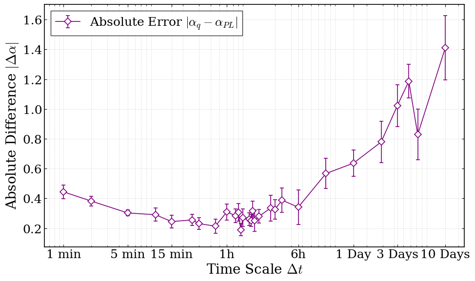
Comparing the tail parameters derived from the pure power-law fit and the asymptotic q-Gaussian approximation reveals significant differences, as shown in Fig. 11. A consistent pattern emerges across all three scenarios: at high-frequency scales, the q-Gaussian model underestimates relative to the power law, predominantly in the region where the power law is shown to provide a better fit. At mesoscales (approximately 1 hour), both fits converge to similar values, reaching their lowest absolute difference.
At longer, interday scales, the q-Gaussian model captures aggregational Gaussianity, causing to approach 1 and to increase, as the exponential decay characteristic of a Gaussian distribution would imply that the power-law exponent diverges to infinity (). In contrast, the pure power-law fit fails to capture this effect, which leads it to underestimate the exponent at these macroscopic scales. This demonstrates that even if both distributions are theoretically equivalent in the tail, the distinct fitting methodologies ultimately yield different exponents.
Finally, we believe that our contributions revisit and substantially extend some of the early investigations reported in [12, 33], which at that time were restricted to price changes in the U.S. dollar–German mark exchange rate. Here, the analysis is extended to stock markets and cryptocurrencies and is supported by a much finer and more detailed statistical investigation. These results may provide a useful framework for market analysts, scientists, investors, and other professionals working with economic and financial data. In particular, generalized functions based on () allow for a global description of the data, avoiding an a priori partition into distinct regions and the consequent need to identify distributional cutoffs before carrying out the analysis.
Funding: R. da Silva was partially supported by CNPq under grants 304575/2022-4 (Productivity Fellowship – PQ), 406820/2025-2 (Universal), 408596/2024-4 (INCT–NanoQuantSS), and 444867/2024-4 (CNPq/MCTI/FNDCT). J.R.Iglesias thanks to CNPq by the partial finantial support: 406820/2025-2 (Universal). R. da Silva also acknowledges financial support from FAPERGS (Fundação de Amparo à Pesquisa do Estado do Rio Grande do Sul) under Grant 25/2551-0002529-0.
References
- [1] (1963) The variation of certain speculative prices. The Journal of Business 36 (4), pp. 394–419. External Links: Document Cited by: §1, §3.2.
- [2] (1965) The behavior of stock-market prices. The Journal of Business 38 (1), pp. 34–105. External Links: Document Cited by: §1, §3.2.
- [3] (1995) Scaling behaviour in the dynamics of an economic index. Nature 376, pp. 46–49. External Links: Document Cited by: §1, §3.2.
- [4] (2001) Empirical properties of asset returns: stylized facts and statistical issues. Quantitative Finance 1 (2), pp. 223–236. External Links: Document Cited by: §1, §3.2, §3.2.
- [5] (2010) Stock markets and criticality in the current economic crisis. Physica A 389, pp. 5460–5467. Cited by: §1.
- [6] (2000) Generalized thermostatistical description of intermittency and non-extensivity in turbulence and financial markets. arXiv preprint cond-mat/0010435. Cited by: §1, §1.
- [7] (1996) The stable paretian hypothesis and the frequency of large returns: an examination of major german stocks. Applied Financial Economics 6 (6), pp. 463–475. External Links: Document Cited by: §1, §3.2.
- [8] (2005) Empirical distributions of stock returns: between the stretched exponential and the power law?. Quantitative Finance 5 (4), pp. 379–401. External Links: Document Cited by: §1, §3.2.
- [9] (2009) Power-law distributions in empirical data. SIAM review 51 (4), pp. 661–703. Cited by: §1, §3.2, §4.1, §4.1.
- [10] (2011) Power law distribution in high frequency financial data? an econometric analysis. Physica A 390, pp. 4433–4444. Cited by: §1.
- [11] (1988) Possible generalization of boltzmann–gibbs statistics. Journal of Statistical Physics 52 (1–2), pp. 479–487. External Links: Document Cited by: §1.
- [12] (1999) Nonextensive statistics: theoretical, experimental and computational evidences and connections. Brazilian Journal of Physics 29 (1), pp. 1–35. Cited by: §1, §1, §5.
- [13] (2003) Nonextensive statistical mechanics and economics. Physica A: Statistical Mechanics and its Applications 324 (1–2), pp. 89–100. External Links: Document Cited by: §1.
- [14] (2005) Bridging a paradigmatic financial model and nonextensive entropy. Europhysics Letters 69 (6), pp. 893–899. External Links: Document Cited by: §1.
- [15] (2002) A theory of non-gaussian option pricing. Quantitative Finance 2 (6), pp. 415–431. Cited by: §1.
- [16] (2008) On a q-central limit theorem consistent with nonextensive statistical mechanics. Milan Journal of Mathematics 76 (1), pp. 307–328. External Links: Document Cited by: §1.
- [17] (1999) Scaling of the distribution of fluctuations of financial market indices. Physical Review E 60, pp. 5305–5316. External Links: Document Cited by: §3.2, §3.2.
- [18] (1999) Scaling of the distribution of price fluctuations of individual companies. Physical Review E 60, pp. 6519–6529. External Links: Document Cited by: §3.2, §3.2.
- [19] (2003) A theory of power-law distributions in financial market fluctuations. Nature 423, pp. 267–270. External Links: Document Cited by: §3.2.
- [20] (2013) Aggregational gaussianity and barely infinite variance in financial returns. Journal of Empirical Finance 20, pp. 102–108. External Links: Document Cited by: §3.2.
- [21] (1933) Sulla determinazione empirica di una legge di distribuzione. Giornale dell’Istituto Italiano degli Attuari 4, pp. 83–91. Cited by: §3.9.2.
- [22] (1928) On the composition of elementary errors: second paper: statistical applications. Skandinavisk Aktuarietidskrift 11 (1), pp. 141–180. External Links: Document Cited by: §3.9.3.
- [23] (1952) Asymptotic theory of certain “goodness of fit” criteria based on stochastic processes. The Annals of Mathematical Statistics 23 (2), pp. 193–212. External Links: Document Cited by: §3.9.4.
- [24] (1989) Likelihood ratio tests for model selection and non-nested hypotheses. Econometrica 57 (2), pp. 307–333. External Links: Document Cited by: §3.10.
- [25] (1979) Bootstrap methods: another look at the jackknife. The Annals of Statistics 7 (1), pp. 1–26. External Links: Document Cited by: §3.11.
- [26] (1980) Stock returns and the weekend effect. Journal of Financial Economics 8 (1), pp. 55–69. External Links: Document Cited by: §4.1.1.
- [27] (1985) An investigation of transactions data for NYSE stocks. The Journal of Finance 40 (3), pp. 723–739. External Links: Document Cited by: §4.1.1.
- [28] (1985) Intraday and overnight returns and day-of-the-week effects. Journal of Financial Research 8 (2), pp. 119–126. External Links: Document Cited by: §4.1.1.
- [29] (1986) A transaction data study of weekly and intradaily patterns in stock returns. Journal of Financial Economics 16 (1), pp. 99–117. External Links: Document Cited by: §4.1.1.
- [30] (2018) Scaling properties of extreme price fluctuations in bitcoin markets. Physica A: Statistical Mechanics and its Applications 510, pp. 400–406. External Links: Document Cited by: §4.2.
- [31] (2018) Statistical properties and multifractality of bitcoin. Physica A: Statistical Mechanics and its Applications 506, pp. 507–519. External Links: Document Cited by: §4.2.
- [32] (2018) Bitcoin market route to maturity? evidence from return fluctuations, temporal correlations and multiscaling effects. Chaos 28 (7), pp. 071101. External Links: Document Cited by: §4.2.
- [33] (1999) Intermittency and nonextensivity in turbulence and financial markets. arXiv preprint cond-mat/9907348. Cited by: §5.