Multiple Nonlinear Waves by (Quantum) Neural Networks:
Checking the AI supremacy
Abstract
To test the potential of so-called quantum physics-informed neural network (QPINN) technology for solving evolutionary partial differential equations, we consider the problem of multiple wave propagation in a weakly nonlinear medium described by the Korteweg-de Vries equation with periodic boundary conditions. Although this problem is solvable analytically, high-genus solutions could represent a rather challenging testbed for numerical methods. Therefore, our idea is to test whether a QPINN is sufficiently mature for application in this context by providing a set of indicators of merit and performing several numerical experiments.
Keywords:
Machine Learning , Integrable Systems , Physics Informed Neural Network , Quantum Machine Learning1 Introduction
In recent years, many deep Neural Networks focused on the study of nonlinear Evolution Differential Equations (PDEs), such as the Physics-Informed Neural Networks (PINN) (Raissi et al., 2017; Raissi et al., 2019; Cuomo et al., 2022). This approach distances itself both from the traditional applications of Machine Learning (ML) techniques and from the much better-known analytical/numerical methods of PDEs. In fact, on the one hand, because of the explosive growth of available data and computing resources, the ML has been promoted from regression to classification problems and it has been shown that deep neural networks can be used as general function approximator (Hornik et al., 1989; Scarselli and Chung Tsoi, 1998). While traditional machine learning can be trained from (possibly labeled) data without knowing the underlying mechanism that produced it, physical system modeling, by contrast, relies on general theoretical principles and (differential) equations for specific dynamical variables that are generally known, in some cases even long ago. Under certain approximations, the equations of motion can be expressed in linear form, whose solutions can be obtained with well-known methods. However, most differential equations are nonlinear and their solutions can exhibit chaotic behavior, irregular and sensitive dependence on initial conditions and, generally, cannot be expressed analytically. However, several nonlinear evolution problems have been solved with analytical and numerical methods, profoundly clarifying their geometric meaning. This is especially true for fully integrable systems (Ablowitz and Segur, 1981; Ablowitz and Clarkson, 1991; Dunajski, 2024), mainly in 1+1 and 2+1 dimensions. But a lot remains of difficult cases to effectively solve, like the celebrated (1+1)D Kuramoto-Sivashinsky equation (Hyman and Nicolaenko, 1986), the 3D Navier-Stokes equation (Protas, 2022), the (N+1)D NonLinear Schroedinger (Kenig and Merle, 2006) and the analogous complex Ginzburg-Landau equation (Aranson and Kramer, 2002), the 4D Yang-Mills system (Beiner, ) and infinitely many other equations. Moreover, also in the case of the completely solvable or integrable PDEs, perturbations and boundary conditions may introduce non integrable effects. So special studies are required in such a cases. Thus, new mathematical tools, including machine learning, may be useful in investigating certain classes of solutions.
In this context, in a first step (Raissi et al., 2017) a PINN has been proposed to solve evolutionary nonlinear partial differential equations. Then, the soliton solutions of KdV, mKdV and KdV-Burgers equation were studied by using the PINN method (Li and Chen, 2020). A little later (Jagtap et al., 2020) the PINN method was enriched by of local conservation laws on discrete domain to solve Burgers and KdV equations. Then, the NLS equation was discussed in terms of the PINN approach by (Yin et al., 2021) and in particular rogue waves in the defocusing case was studied (Wang and Yan, 2021).
The main strategy of PINN is to minimize an appropriate loss function for the NPDE-related configurational variables, evaluated at the initial/boundary sampling points and on the evolution domain. In this way, the PINN method can provide feedback on the optimal parameters of the neural network. These requirements can be strengthened by imposing loss functions that involve any local NPDE conservation laws (Raissi et al., 2020; Lin and Chen, 2022; Fang et al., 2022).
The existence of conservation laws is particularly relevant in the case of fully integrable systems, as an infinite number of them can be found in commutation with each other. This aspect, however, has not yet been implemented. Furthermore, in such particular cases, Hamiltonian and bi-Hamiltonian structures emerge, opening up further possibilities for implementing numerical calculations and simulations, including PINN techiques. In any case, the key feature of integrable partial differential equations is that they are compatibility conditions for certain linear operators (Lax pairs). Analysis of the corresponding spectra leads to the identification of suitable separate variables, whose time evolution can be determined via quadratures. This allows for the writing of appropriate formulas for entire classes of global solutions. It is clear that in these situations, the machine learning approach offers no advantage in principle over analytical resolution, or its numerical transposition, unless there are significant difficulties in implementing the aforementioned formulas. These methods can be quite complex if they involve the calculation of numerous nonlinear modes (oscillations), which typically decompose into an exponentially large number of normal harmonic modes. Therefore, the first aspect we wish to explore in this work is whether the PINN approach is robust enough with respect to the complexity of the initial and boundary data, even for a well-known, fully integrable system. In particular, we chose to study the typical behavior of PINNs with respect to the propagation of multiple nonlinear waves (Stokes waves or cnoidal waves), described in the Korteweg-de Vries (KdV) model by higher-genus finite-gap solutions (Dubrovin et al., 1976; Dubrovin, 1981; Belokolos, 1994).
Such a kind of problem is relevant in our context since: 1) the initial and boundary conditions are not trivial at all, 2) a formal analytic solution exists in terms of Riemann Theta functions, but it may involve an exponentially large number of harmonic components in order to get a numerically meaningful solution, 3) alternatively numerical solutions may be expressed in terms of a smaller, but sufficiently large, number of hyperelliptic functions (Frauendiener and Klein, 2004; Trogdon and Deconinck, 2013) or by solving high order Riemann-Hilbert problems (Bilman et al., 2022) , 4) a quite generic initial problem for KdV may involve nonlinear superposition of solitons and cnoidal waves, 5) experimental data reported the nonlinear superposition of hundred of nonlinear wave components (Osborne, 2010).
For these studies, the analysis began using the standard PINN method. However, several different routes are possible. Certainly, the one involving conservation laws is mandatory. On the other hand, modern machine learning techniques also hope to benefit from quantum computing, which promises to speed up the most complex computational tasks by exploiting the nonlocal correlations between entangled qubits. This perspective is strongly supported by several studies (Schuld and Petruccione, 2018; Pastorello and others, 2023; Du et al., 2025), which currently have relatively few hardware implementations, but which could be very interesting even in the current NISQ era (Preskill, 2018).
In particular, we compared the classical PINN method with a quantum version of the neural networks (QPINN) based on Variational Quantum Algorithm (VQA) (Benedetti et al., 2019; Trahan et al., 2024; Jaderberg et al., 2024; Schuld and Petruccione, 2018).
The VQA were introduced for complex chemical calculations (Peruzzo et al., 2014). Applications such as simulating complicated quantum systems or solving large-scale linear algebra problems are very challenging for classical computers, owing to the extremely high computational cost. Quantum computing promises a solution, although fault-tolerant quantum computers will probably not be available in the near future. Current quantum devices have serious limitations, including low numbers of qubits and noise processes that limit circuit depth. VQAs have emerged as a leading strategy for addressing these constraints and use classical optimizers to control parameterized quantum circuits. VQAs have now been proposed for essentially all applications that researchers have envisaged for quantum computers, and they appear to be the best hope for obtaining quantum advantage. Nevertheless, challenges remain, including the trainability, accuracy and efficiency of VQAs.
In this work, we compared the capabilities of a QPINN with respect to a PINN in the study of specific PDEs solutions, highlighting the fact that a reduction in the number of variational parameters is typically achieved.
Therefore, our main goals in this work can be summarized as follows: 1. To use (Q)PINNs in large systems, where standard numerical techniques become computationally expensive and unstable; 2. To provide a standard tool for comparing relative performance by training (Q)PINNs on fully integrable systems before applying them to more general and less structured evolutionary partial differential equations.
The article is organized, after this Introduction, with Section 2 summarizing the most relevant results from the theory of multiperiodic KdV solutions. Section 3 summarizes the main characteristics of a PINN algorithm and subsequently of a QPINN. Section 4 illustrates the details of the calculations performed on some examples of genus 2, 3, and 5 waves, using both PINN and QPINN. Finally, Section 5 draws some conclusions from comparisons between the various examples reported and, more importantly, opens up new avenues for further investigation.
2 Multi-periodic solutions of the KdV
The celebrated Korteweg - de Vries equation (KdV) for the real field reads (Ablowitz and Segur, 1981)
| (1) |
It is a universal model for conservative dispersive non linear waves. For instance, it arises as a model for Non Linear Waves in Shallow Water (Whitham, 1974), but it playes a role also in quantum gravity (Okuyama and Sakai, 2020).
The key property for solving the KdV equation consists in the so-called Lax representation (Ablowitz and Segur, 1981):
| (2) | |||
| (3) |
The Schrödinger operator over allows to perform the mapping
KdV data spectral data ,
where understands for Inverse Spectral Transform. Precisely, in solving the problem with regular initial conditions with rapidly vanishing potentials , the following chain of three linear problems has to be performed: Here the Direct Prob. understands the Schroedinger operator scattering problem for the potential , described in the momentum complex plane . While by Inverse Prob. we indicate the solution of the Gelfand-Marchenko equation (Ablowitz and Segur, 1981). For reflectionless potentials (), one obtains the well-kown -soliton Hirota formula
| (4) | |||||
The computational complexity of such a formula is basically related to that one of the computation of the determinants, that is , but instabilities can occur in the asymptotic regions and . On the other hand, solving the initial data problem may results intriguing, mainly to prove reflectionless property of the potential. However, about such a topic there exists a wide literature (Ablowitz and Segur, 1981; Matveev and Salle, 1992).
On the other hand, one can pose the question of periodic potentials . This problem was approached by the classical Floquet theory for the time-independent Schrödinger equation (Dubrovin et al., 1976; Dubrovin, 1981; Belokolos, 1994).
Summarizing the main results, one looks at the matrix eigenfunction solution
| (5) |
of the Schroedinger equation with the initial periodic potential and "energy" eigenvalue , namely
| (6) |
The matrix is normalized at the point as follows
| (7) |
The periodicity of the potential implies the existence of a monodromy matrix such that
| (8) |
which, in its turn, defines the so-called main spectrum
| (9) |
The set of gaps determines forbidden zones for the existence of bounded regular solution to the system (6). If , is called a finite-gap potential of genus , and these are of greater interest to physics. For values of outside the gaps, the scalar wavefunctions are meromorphic on the two-sheeted Riemann surface covering the -plane
| (10) |
The wavefunctions have a simple pole in the complex -plane, located in the band-gaps at . The ends of the gap zones are branch-points. The following relations hold
| (11) |
where denotes the Wronskian of its arguments and are the so called hyperelliptic functions. Their values and the sheet where the poles are located complete the entire set of spectral data, together with the main spectrum (9).
The asymptotic series expansion in inverse power of , in right hand side of expression (11), allows to determine completely the evolution on time of the functions . Thus, one is led to the following compatible system
| (12) |
| (13) |
where and represent and derivative, respectively.
In the above formulation, the Inverse Spectral Transform for periodic potentials is given by the solution of the two separated ODEs systems presented in (13), sometimes called the Dubrovin curve. For the equation for correspond to uniform translation of a suitable Weierstrasse elliptic function. But already for the ODE system is challenging to be explicitely solved (Dubrovin et al., 1976) and numerical techniques are required for higher (Trogdon and Deconinck, 2013; Bilman et al., 2022).
On the other hand, Dubrovin discovered an implicit way to linearize the problem (13) in general, by using the algebraic geometry. The first step is to introduce on the elliptic curve (10) a family of non contractible oriented curves encircling the gap bands, or going from one sheet to the other one by crossig the gap band. They form a homotopy group and a base of such curves are cycles denoted by . A dual description is provided by a canonical bases of holomorphic differentials on
| (14) |
normalized in such a way
| (15) |
Thus one can introduce the symmetric matrix of periods with entries
| (16) |
The matrix has negative real part . Thus, the matrix allows to build the Riemann Theta function associated to the Rimannian surface , namely
| (17) |
where , and are suitable constant -component vectors belonging to .
The function is quasi-N-multiperiodic, in the sense that the relation
| (18) |
holds for any arbitrary -components vectors of integers and .
Then, the main result is that a -multi-periodic solution of the KdV equation (1) is expressed by
| (19) |
where the components of the variable introduced in (17) are specified by the so-called Abel map
| (20) |
in terms of the spectral data. This is a fundamental relationship between the solution in terms of hyperelliptic functions (12) and the one (19) in terms of the Riemann , or in Fourier expansion form, if it preferred. Both formulations are very useful, but each of them has computational limitations. From one side, the computation of the hyperelliptic functions is challenging, on the other hand the Fourier components to sum up increases exponentially with the genus N.

In order to be more explicit, the Riemann function of genus can be written as
| (21) | |||||
| (22) | |||||
| (23) |
where the last relation in (23) is specific of the KdV equation. So, even if the wave-vectors are commensurables, the same does not holds for the frequency vectors .
In the special case , the Riemann reduces to the Jacobi function. In fact, taking the definition (17) defined as
| (24) |
where
Setting with denoting the complete elliptic integral of first kind of module , one derives the KdV cnoidal solution
| (25) | |||||
Remarkably, the linear dispersive waves are the small amplitude limit
On the other hand, the limit of the expression (25) will lead to the 1-solitonic solution by the Hirota formula (4). Of course, the nonlinear one mode is the simplest and a very special case.
In principle, from an initial data point, one should derive the entire Riemann spectrum, i.e., the principal spectrum , i.e., the period matrix , and the phases. However, in general, this requires the use of several advanced numerical techniques. Note that in several concrete circumstances (see, for example, (Osborne, 2010)), hundreds of nonlinear modes overlap and interact. In typical experimental situations, the amount of computational resources required becomes an issue.
3 Briefs about standard numerical approaches for higher genus solutions
A first approach in numerical integration of the periodic KdV equation for given initial and boundary data consists in solving the system (12-13) in the following steps.
- 1.
One provides a space/time discretization of the domain by a lattice of points.
- 2.
Chose the genus value
- 3.
At , the initial data are given by the band edges of the hyperelliptic surface: and by the initial conditions for the hyperelliptic functions at the specific point .
- 4.
The integration procedure begins providing by solving the Cauchy problem
- 5.
At any space lattice site , perform the time integration of
for from the initial datum
- 6.
Update the value of the KdV solution
on the discretized lattice.
- 7.
Repeat the procedure from 5. while , then print .
The above equation where numerically studied in (Osborne, 2010; Frauendiener and Klein, 2004). In (Trogdon and Deconinck, 2013; Bilman et al., 2022) a differet approach was adopted.
4 PINN and QPINN methodology
Rewriting (1) in the generic form of an evolutive nonlinear 1-space dimensional PDE
| (26) |
where represents a nonlinear differential polynomial of the dependent variable w.r.t. . For sake of simplicity here we consider only constant coefficients w.r.t. the independent variables . The previous equation is supplemented with initial and boundary conditions:
| (27) | ||||
| (28) |
In this notation is a boundary operator (for instance the Dirichlet, or the Neumann boundary conditions, but also mixed or other types are possible).
The left hand side in (26) is a function in the jet space of the variables , which order equals the highest derivative appearing in . Thus, it is natural to introduce for any indexed family of elements the residual function
| (29) |
The best approximation for the solution of (1) can obtained by minimizing the Loss function
| (30) |
over the set of data used for the supervised training. The index here is understood as the set of trainable network parameters optimizing the approximation.
Explicitly writing out the individual terms of the Loss function one has:
- 1.
Mean square error of residual
(31) - 2.
Mean square error for initial condition
(32) - 3.
Mean square error for boundary condition (both Dirichlet and Neumann)
(33) (34)
4.1 Details about PINN calculations
The architecture used in this work is based on a relatively simple deep feed-forward neural networks architectures with hyperbolic tangent activation functions. The feedforward neural network called Multilayer Perceptron (MLP) is a parametrized approximator of functions
| (35) |
where, in our calculations, the tensor type input data is passed to a series of hidden layers with neurons for each layer.
Setting , the MLP is recursively defined by
| (36) |
Then, the final output layer yields
| (37) |
In the adopted notation above is the weight matrix in l-th layer, thus collectively represents all trainable parameters in the network.
Furthermore, the symbol denotes an element-wise activation function, which for our network is the hyperbolic tangent (Tanh).
Minimization of is made by performing an iterative gradient descent algorithm. Where, at the -th iteration, the trainable parameter is updated according to
being the learning rate and the gradients are calculated by using the Backward Automatic Differentiation method. Such a kind of algorithm is called Adam (Kingma and Ba, 2014).
4.2 Details about QPINN calculations
The architecture of the Quantum PINN is a modification of the classical one, where one hidden layer is replaced by a quantum node, simulated by resorting to the Pennylane library (Bergholm and et al., 2018). The quantum node is structured in a series of three different tools: i) the quantum data encoding of classical inputs (the quantum feature map), ii) a unitary quantum variational layer composed by a set of single-qubit parametric rotations alternated by a corresponding set of qubits entanglement operators, iii) a projective measurement apparatum. In our architecture we used variational layers of qubit embedded in the classical layers.
The quantum variational layer tunable parameters are the angles in the rotations. The entanglement is realized with the CNOT gate between nearby qubits in a closed chain. A prototypical example of a such type is drawn in Fig.2
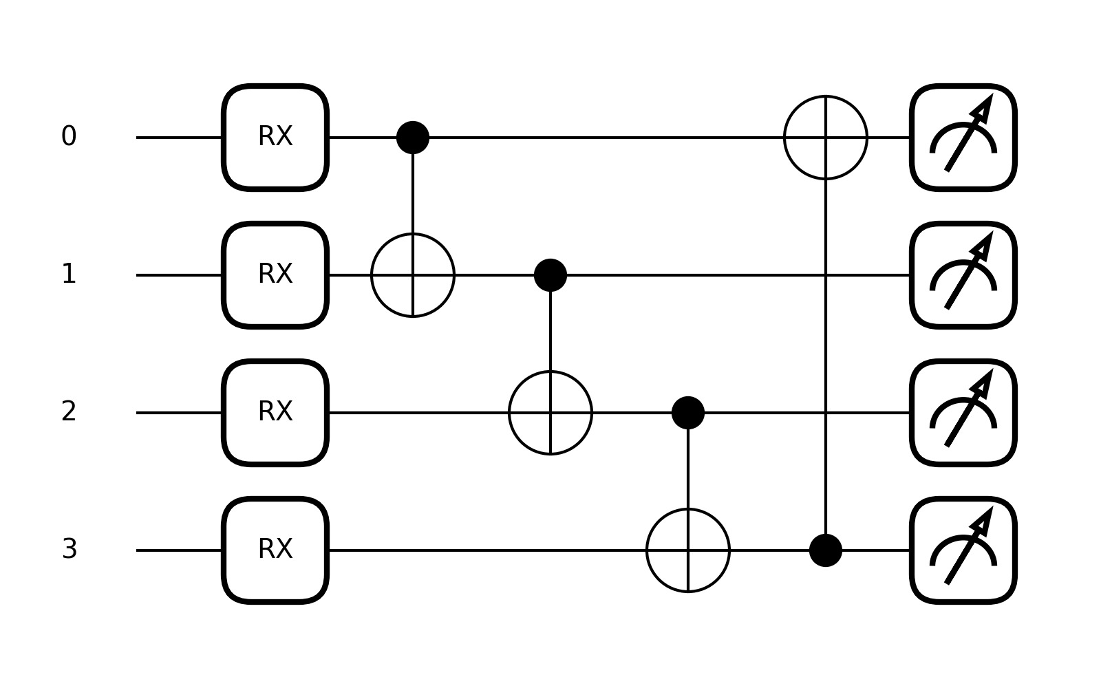
but other architectures are possible.
To produce a quantum parameterized output to add to the other "classical" parameters of the network, the qnode workflow is
- 1.
Initialize the quantum state
- 2.
Traslate the classical data , being the number of input features, by a suitable Angle Map and generate the quantum state
- 3.
Apply the variational circuit providing
- 4.
Measure the observable
- 5.
Output from the network ; .
The simulations performed in the present work used the Pennylane functions AngleEmbedding, to yield the state, and BasicEntanglerLayers in order to entangle the qubits.
Since currently does not exists an efficient quantum algorithm for computing derivatives, the parameters introduced by the qnode will enter in the Loss function (30) at the same foot of those coming from the classical layers. This leads to the idea of the hybrid training of variational algorithms, in which queries to a quantum device are optimized by a classical algorithm. The updated parameters are fed back to the quantum hardware in a closed loop, defining at each iteration a new quantum circuit.
The simulations performed in the present work do not take account of quantum noise effects.
5 Results Analysis

For the simulations we have used a time domain and a space domain . The numerical solutions were obtained by using standard integration methods for the Dubrovin’s curve (13). But, for convenience, the input data were normalized inside the neural network, both for space and time to be in the range by the relation
| (38) |
The training consist in Adams epochs, followed by LBFGS iterations. The latter belongs to the family of second-order quasi-Newtonian methods, i.e., based on the calculation of the Hessian matrix (Liu and Nocedal, 1989).
Below the table of the sampling points used to train the neural network:
| Sampling points | |
|---|---|
| PDE | , |
| IC () | , |
| BC value in | , |
| BC value in | , |
| BC deriv. | , |
| BC deriv. | , |
Generalization means to compute the values of the function in points not belonging to the sampling points and compare them with the true values of the numerical solution of (1). We proved this integration method for different but small genus configurations. Among several experiments, here we are going to show the results (see Fig.1 and Fig.3) concerning two particular choices, being meaningful representatives of total set:
- 1.
case:
Spectral endpoints
Auxiliary spectrum - 2.
Spectral endpoints . Auxiliary spectrum
For the PINN case with the aforementioned architecture, we summarize the final losses, the relative error with respect to the exact numerical solution defined by and the total number of trainable parameters in the following table:
| genus | 2 | 3 |
|---|---|---|
| Final Loss | 6,0597e-02 | 1.5073e+00 |
| error | 1,286e-01 | 2.912e-01 |
| Parameters | 10.001 | 10.001 |
For the QPINN approach, after replacing one hidden layer with a quantum node for qubits and variational layers, the corresponding results are
| genus | 2 | 3 |
|---|---|---|
| Final Loss | 1.4359e-01 | 1,9714e+00 |
| error | 1,342e-01 | 3.671e-01 |
| Parameters | 8.571 | 8.571 |
Furthermore, we have studied the variations of the relative error as a function of the number of layers ad neurons, both in the classical ad quantum approach.
6 Conclusions and Perpectives
From the study reported above we can draw some preliminary conclusions.
We have shown that it is possible to use (Q)PINNs in systems with a certain degree of complexity, here represented by the genus of the periodic KdV solutions sought. However, at the stage of this work, is still small, while we are interested in its values at least in the tens if not hundreds, where standard numerical techniques quickly become computationally expensive and unstable. This somewhat fulfills the goal 1. set in the Introduction. However, for the proposed architectures of neural network the typically fluctuates in the range . Thus, the accuracy of the computations is not yet well established.
Comparing the previous tables, we see that QPINNs can significantly reduce the number of network parameters. However, the quality in terms of the metric is slightly lower than the corresponding PINN in our scheme. In any case the relation among architecture - number of parameters - genus- relative error is far to be completely investigated and understood.
Another aspect not yet considered is the evaluation of the minimal sampling points number required by both (Q)PINN architectures in relation with a given .
We noticed also that the constructed (Q)PINNs are unstable at times greater than the training time domain. Furthermore, the stability of the network with respect to variations in the initial and boundary data parameters (, , ) needs to be verified.
These are the basic problems to be solved in order to establish an effective advantage of the ML techniques with respect the analytical numerical one in the context of the studies about the evolutive PDEs. Since in our research we are comparing the PINN approach with analytical very well controlled contexts, it is much harder to make definitive statements in the case of non integrable equations.
Analogously, it is still difficult to evaluate the effective advantages of the quantum ML, for a long series of arguments. First of all, during the training the computational speed of the quantum algorithm on a classical computer is quite slow in comparison with true quantum computations.
On the other hand, currently the implementation of variational quantum circuits is feasible with the NISQ quantum devices. Thus, the above problem can be directly evaluated and it is i the program of our future researches.
Differently, the implementation of the gradient descent algorithm on quantum hardware is still a hot research topic. Thus, the algorithm’s architecture will remain hybrid for a long time to come.
Thus, several aspects in the training of (Q)PINNs are largely to be investigated, so that tests on fully integrable systems could provide a standard tool for comparing their relative performance, before applying them to non-integrable cases.
Concerning the completely integrable systems, in particular the KdV equation, a very promising direction of investigation is to use the formulation of the Inverse Problem in terms of Riemann-Hilbert problem on the complex plane of the spectral parameter. This approach was implemented in numerical algorithms (Trogdon and Deconinck, 2013; Bilman et al., 2022) able to manage solutions with higher than previously. From point of view of the (Q)PINN approach this is a true challenge in terms of effectiveness of the method. This is the topic which we are currently studying.
Finally, another direction of investigation is to use (Q)PINN to compute spectral data for very complex cases observed in Nature. Indeed, this mathematical problem is analogous to, but much more extensive than, the Fourier transform method for linear PDEs. However, to our knowledge, there is currently no conventional quantum algorithm, such as the Quantum Fourier Transform, that significantly speeds up these calculations. Therefore, an alternative method could be a good contender.
Acknowledgements
ML thanks the MMNLP project of the INFN for partially supporting this project.
References
- Solitons, nonlinear evolution equations and inverse scattering. London Mathematical Society Lecture Note Series, Cambridge University Press. Cited by: §1.
- Solitons and the inverse scattering transform. SIAM. Cited by: §1, §2, §2, §2, §2.
- The world of the complex ginzburg-landau equation. Rev. Mod. Phys. 74, pp. 99–143. External Links: Document, Link Cited by: §1.
- [4] THE yang-mills equations: a pde perspective. External Links: Link Cited by: §1.
- Algebro-geometric approach to nonlinear integrable equations. Algebro-geometric Approach to Nonlinear Integrable Equations, Springer-Verlag. External Links: ISBN 9783540502654, LCCN 94019255, Link Cited by: §1, §2.
- Parameterized quantum circuits as machine learning models. Quantum science and technology 4 (4), pp. 043001. Cited by: §1.
- PennyLane: automatic differentiation of hybrid quantum-classical computations. arXiv:1811.04968. Cited by: §4.2.
- Computation of large-genus solutions of the korteweg-de vries equation. ArXiv abs/2205.00153. External Links: Link Cited by: §1, §2, §3, §6.
- Scientific machine learning through physics–informed neural networks: where we are and what’s next. Journal of Scientific Computing 92 (3), pp. 88. External Links: Document, ISBN 1573-7691, Link Cited by: §1.
- A gentle introduction to quantum machine learning. Springer Nature. External Links: Document Cited by: §1.
- Theta functions and non-linear equations. Russian Mathematical Surveys 36 (2), pp. 11. External Links: Document, Link Cited by: §1, §2.
- Non-linear equations of korteweg-de vries type, finite-zone linear operators, and abelian varieties. Russian mathematical surveys 31 (1), pp. 59. Cited by: §1, §2, §2.
- Solitons, instantons, and twistors. Oxford University Press. External Links: ISBN 9780198872535, Document, Link Cited by: §1.
- Data-driven soliton solutions and model parameters of nonlinear wave models via the conservation-law constrained neural network method. Chaos, Solitons & Fractals 158, pp. 112118. External Links: ISSN 0960-0779, Document, Link Cited by: §1.
- Hyperelliptic theta-functions and spectral methods. Journal of computational and applied mathematics 167 (1), pp. 193–218. Cited by: §1, §3.
- Multilayer feedforward networks are universal approximators. Neural Networks 2 (5), pp. 359–366. External Links: ISSN 0893-6080, Document, Link Cited by: §1.
- The kuramoto-sivashinsky equation: a bridge between pde’s and dynamical systems. Physica D: Nonlinear Phenomena 18 (1), pp. 113–126. External Links: ISSN 0167-2789, Document, Link Cited by: §1.
- Let quantum neural networks choose their own frequencies. Phys. Rev. A 109, pp. 042421. External Links: Document, Link Cited by: §1.
- Conservative physics-informed neural networks on discrete domains for conservation laws: applications to forward and inverse problems. Computer Methods in Applied Mechanics and Engineering 365, pp. 113028. External Links: ISSN 0045-7825, Document, Link Cited by: §1.
- Global well-posedness, scattering and blow-up for the energy-critical, focusing, non-linear schrödinger equation in the radial case. Inventiones mathematicae 166 (3), pp. 645–675. External Links: ISSN 1432-1297, Link, Document Cited by: §1.
- Adam: a method for stochastic optimization. arXiv preprint arXiv:1412.6980. Cited by: §4.1.
- A deep learning method for solving third-order nonlinear evolution equations. Communications in Theoretical Physics 72 (11), pp. 115003. External Links: Document, Link Cited by: §1.
- A two-stage physics-informed neural network method based on conserved quantities and applications in localized wave solutions. Journal of Computational Physics 457, pp. 111053. External Links: ISSN 0021-9991, Document, Link Cited by: §1.
- On the limited memory bfgs method for large scale optimization. Mathematical programming 45 (1), pp. 503–528. Cited by: §5.
- Darboux transformations and solitons. External Links: Link Cited by: §2.
- JT gravity, kdv equations and macroscopic loop operators. Journal of High Energy Physics 2020 (1), pp. 156. External Links: Document, ISBN 1029-8479, Link Cited by: §2.
- Nonlinear ocean waves and the inverse scattering transform. International Geophysics, Academic Press. External Links: ISBN 9780080925103, Link Cited by: §1, §2, §3.
- Concise guide to quantum machine learning. Springer. External Links: Document Cited by: §1.
- A variational eigenvalue solver on a photonic quantum processor. Nature Communications 5 (1), pp. 4213. External Links: Document, ISBN 2041-1723, Link Cited by: §1.
- Quantum Computing in the NISQ era and beyond. Quantum 2, pp. 79. External Links: Document, Link, ISSN 2521-327X Cited by: §1.
- Systematic search for extreme and singular behaviour in some fundamental models of fluid mechanics. Philosophical Transactions of the Royal Society A: Mathematical, Physical and Engineering Sciences 380 (2225), pp. 20210035. External Links: ISSN 1364-503X, Document, Link Cited by: §1.
- Physics-informed neural networks: a deep learning framework for solving forward and inverse problems involving nonlinear partial differential equations. Journal of Computational Physics 378, pp. 686–707. External Links: ISSN 0021-9991, Document, Link Cited by: §1.
- Physics informed deep learning (part i): data-driven solutions of nonlinear partial differential equations. arXiv preprint arXiv:1711.10561. Cited by: §1, §1.
- Hidden fluid mechanics: learning velocity and pressure fields from flow visualizations. Science 367 (6481), pp. 1026–1030. External Links: Document, Link Cited by: §1.
- Universal approximation using feedforward neural networks: a survey of some existing methods, and some new results. Neural Networks 11 (1), pp. 15–37. External Links: ISSN 0893-6080, Document, Link Cited by: §1.
- Supervised learning with quantum computers. Quantum science and technology 17. Cited by: §1, §1.
- Quantum physics-informed neural networks. Entropy 26 (8), pp. 649. Cited by: §1.
- Numerical computation of the finite-genus solutions of the korteweg–de vries equation via riemann–hilbert problems. Applied Mathematics Letters 26 (1), pp. 5–9. Cited by: §1, §2, §3, §6.
- Data-driven rogue waves and parameter discovery in the defocusing nonlinear schrödinger equation with a potential using the pinn deep learning. Physics Letters A 404, pp. 127408. External Links: ISSN 0375-9601, Document, Link Cited by: §1.
- Linear and nonlinear waves. Pure and applied mathematics, J. Wiley. External Links: ISBN 0471940909 Cited by: §2.
- Data-driven femtosecond optical soliton excitations and parameters discovery of the high-order nlse using the pinn. Nonlinear Dynamics 105, pp. 603–616. External Links: ISSN 1573-269X, Link, Document Cited by: §1.