GeoAgent: Evaluating VLM Geolocalization Through Embodied Navigation
Abstract
Modern Vision-Language Models (VLMs) perform well above the human baseline in image geolocalization, a task critically important in disaster response, OSINT verification, and location privacy. However, most efforts to study AI behavior on the task remain limited to static image-based retrieval, classification, and predictions. We argue that faithful recreation of the task should involve embodied navigation, where a multimodal agent autonomously explores its surroundings to gather observations before submitting a prediction. To this end, we introduce GeoAgent, an agentic environment-based benchmark that requires agents to navigate Street View environments to refine their geolocalization through sequential reasoning. Our analysis shows that modern VLMs struggle to discern regional patterns while succeeding at country- and continent-level predictions. When compared to static image-based baselines, agentic navigation significantly improves accuracy across established metrics. We also note severe bias in a developed/developing region context across frontier model architectures and poor self-improvement capabilities given incorrect priors. Overall, our work establishes the challenges of embodied navigation and geospatial reasoning. We publicly release our code and the GeoAgent environment: https://geoagent-benchmark.github.io
1 Introduction
Geolocalization from visual inputs has emerged as a challenging spatial reasoning task for modern AI systems. Among various tests, the popular game GeoGuessr11 1 https://www.geoguessr.com attracts the most attention Haas et al. (2024); Cheng et al. (2025); Talreja et al. (2026); Wazzan et al. (2024); Jay et al. (2025); Suresh et al. (2018), which requires accurate geospatial predictions within a limited Street View-like navigable environment. Early AI approaches to this game framed GeoGuessr as an image classification task (Haas et al., 2024). More recently, Vision-Language Models (VLMs) have demonstrated remarkable zero-shot performance on geolocalization tasks (Cheng et al., 2025; Yi and Shan, 2025; Zhang et al., 2025; Li et al., 2025a), owing to their web-scale generalizability in interpreting visual cues such as signage, architecture, and vegetation.

Beyond the game, visual geolocalization finds use in many real-world workflows, such as disaster response, where damage-assessment pipelines must localize ground-level photographs of affected areas when GPS metadata are stripped, spoofed, or never recorded Gupta et al. (2019). Further, it also finds usage in OSINT verification, fact-checking Song et al. (2026), autonomous navigation, and robotics. Understanding the limits of this capability is important to prevent misuse (Huang et al., 2025; Li et al., 2025b).
Most existing evaluations assess models on single, static images, which fail to capture how humans actually tackle geolocalization through active exploration of their environment. Vyas et al. (2022) provides richer contextual clues using video clips, but remains a passive observer. Passive inference traps the model in a fixed trajectory: critical identifying features cannot be captured by a constrained set of static images, and the most informative view for a given location may simply not be among them, leaving no room to seek disambiguating evidence. Embodied navigation resolves this bottleneck by letting the agent reason and execute navigational actions, such as movement and rotation, to maximize information gain. This mirrors how human players approach geolocalization and represents an unexplored frontier for evaluating spatial reasoning in VLMs. Evaluating VLMs only under passive inference therefore tests recognition, not reasoning under uncertainty, which is the distinction we achieve with GeoAgent.
Modern advances in tool calling Patil et al. (2025); Yao et al. (2023); Erdogan et al. (2024); Ehtesham et al. (2025); Singh et al. (2025) and agentic web navigation Wu et al. (2025); Deng et al. (2023); Zhou et al. (2023) have made simulating web-based workflows possible. Leveraging these capabilities, we introduce GeoAgent, both an open-source, modular, and reusable agentic environment and a benchmark that evaluates VLMs through embodied navigation in fully explorable Street View environments (Figure 1). The task involves two distinct steps: exploration actions with tool calls and geospatial reasoning for the final location guess. This enables us to study the following research questions that static evaluation does not capture:
- •
RQ1: Do VLMs improve geolocalization accuracy through active exploration, and does improvement depend on the correctness of initial hypotheses?
- •
RQ2: Do frontier VLMs exhibit systematic geographic bias between developed and developing regions?
- •
RQ3: How do exploration strategies differ across VLM architectures, and does action efficiency correlate with task performance?
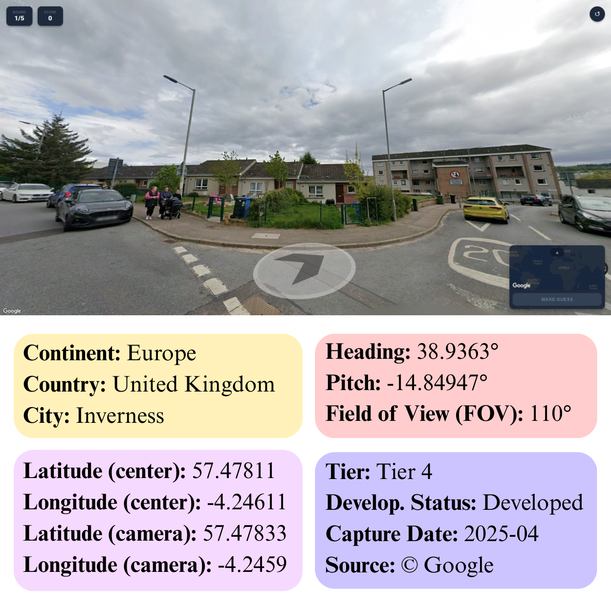
Our benchmark comprises 1,200 fully navigable Street View locations across 100 cities spanning developed and developing regions worldwide, with difficulty stratified by recognizability tiers, as shown in Figure 2. We conduct comprehensive agentic behavioral evaluations of five frontier VLMs plus Geo-R1 7B and compare them to static multiview baselines, revealing that models demonstrate limited self-correction capabilities when initial hypotheses are incorrect. Our analyses also reveal substantial bias among developed and developing geolocations across frontier model capabilities. To the best of our knowledge, our work represents the first comprehensive study of agentic behavior under geospatial embodied navigation constraints. We plan to release our data publicly upon acceptance to promote further research.
2 Related Work
| Tier | # Cities | Samples | Share (%) | Example Cities | Developed | Developing |
|---|---|---|---|---|---|---|
| Tier 1 | 5 | 34 | 2.85 | New York, Tokyo | 5 | 0 |
| Tier 2 | 10 | 86 | 7.14 | Rome, Mumbai | 5 | 5 |
| Tier 3 | 25 | 257 | 21.42 | Bern, Bangalore | 10 | 15 |
| Tier 4 | 25 | 343 | 28.56 | Oulu, Mombasa | 12 | 13 |
| Tier 5 | 35 | 480 | 40.00 | Inuvik, Siem Reap | 14 | 21 |
| Total | 100 | 1,200 | 100.00 | – | 46 | 54 |
| Action | Description |
|---|---|
| ROTATE:<degrees> | Rotate to a specific heading (0–360°) |
| ROTATE_LEFT | Rotate 90° left from current view |
| ROTATE_RIGHT | Rotate 90° right from current view |
| ROTATE_BEHIND | Rotate 180° to look behind |
| LOOK_UP | Tilt the camera up by 20° |
| LOOK_DOWN | Tilt the camera down by 20° |
| MOVE_FORWARD | Move forward along the road or path |
| RETURN_START | Return to the starting position |
| GUESS | Submit the final location guess |
2.1 Vision-based Geolocalization
Early foundational works treated planetary-scale geolocalization as a discrete prediction task. PIGEON (Haas et al., 2024) established state-of-the-art performance using semantic geocell clustering and contrastive pretraining on GeoGuessr data. Yi and Shan (2025) democratized this with GeoLocSFT, achieving competitive results via efficient supervised fine-tuning on small, high-quality datasets (2.7K pairs). Despite their effectiveness, these specialist models operate as black boxes on single static images, lacking interpretability.
To address this, the recent literature uses Vision-Language Models (VLMs) for explicit reasoning. GeoReasoner (Li et al., 2024) employs reasoning-tuning to extract visual cues (e.g., signage, vegetation), while GLOBE (Li et al., 2025a) introduces a bi-objective optimization framework to assess image localizability before predicting. Concurrently, Geo-R1 (Xu et al., 2025) utilizes reinforcement learning to instill a geospatial thinking paradigm, and GeoGuess (Cheng et al., 2025) establishes benchmarks for hierarchical reasoning (Country City). However, evaluations like IMAGEO-Bench (Li et al., 2025b) and FairLocator (Huang et al., 2025) reveal that general-purpose VLMs (GPT-4V and Gemini) exhibit geographic biases in non-Western regions. GAMa (Vyas et al., 2022) substitutes static images with video clips for cross-view geo-localization, yet the observer cannot act to resolve ambiguity. Crucially, all these approaches remain confined to passive inference by analyzing fixed views, unlike GeoGuessr.
2.2 Agentic Web Navigation
Recently, AI evaluation has shifted toward autonomous interaction, primarily in 2D web environments. Benchmarks like WebArena (Zhou et al., 2023) and Mind2Web (Deng et al., 2023) evaluate agents on long-horizon tasks requiring DOM manipulation. Advanced methods have since optimized this agency: Synapse (Zheng et al., 2024) introduces memory-augmented prompting (trajectory-as-exemplar) for complex workflows, RealWorldWebAgent (Gur et al., 2024) employs efficient planner models (HTML-T5), and WebWalker (Wu et al., 2025) focuses on systematic subpage traversal. In the geospatial domain, agency remains nascent. NAVIG (Zhang et al., 2025) introduces limited tool use (map retrieval, knowledge bases), and GeoComp (Song et al., 2026) models human-like deduction chains. However, these geo-agents remain physically static, unable to navigate the environment, while web agents operate in semantic (not spatial) 2D spaces.
GeoAgent bridges this gap by treating geolocation as embodied, interactive exploration. Unlike web agents navigating DOM trees, we formalize navigation actions (movement, rotation) within 3D environments (Google Street View). By evaluating models’ ability to actively reduce uncertainty through physical exploration, we establish a new paradigm for assessing spatial intelligence.
3 Method
3.1 Task Setup & Data Collection
GeoAgent involves a navigable web interface that can be navigated through tool calls to explore the surrounding street signs, vegetation, and architecture for the final guess. We design a minimal interface that simulates navigation environments akin to OpenGuessr22 2 https://openguessr.com with Google Street View. VLMs must autonomously explore a provided environment, explain their observations, and reason through a guess at every step.
A round is one full evaluation instance from a single spawn point in the dataset, played once by one model. An action is one complete agent turn within a round, comprising a rendered viewport screenshot, a model call that returns the structured JSON of Table 2, and the execution of the returned tool call. The terminal GUESS action consumes one action from the budget. The action budget is the maximum number of actions permitted in a round. A model may terminate early by emitting GUESS, and is force-terminated with its current best guess once the budget is exhausted. This makes the exploration setup a guess refinement procedure.
We limit exploration to 8 steps as a principled choice reflecting realistic agentic deployment constraints. Appendix B shows that mean Haversine distance plateaus and occasionally degrades beyond action 5, indicating that agents either commit to a hypothesis early or fail to update it meaningfully. An unconstrained budget does not help LLMs improve (Table 3) and instead amplifies confirmation bias (Appendix B) and inflates API costs (Appendix G) without added diagnostic value.
We initially collected a list of 100 cities across the globe based on two criteria: developed/developing status (according to the UN Council for Trade and Development33 3 https://unctadstat.unctad.org/EN/Classifications.html) and recognizability tiers (as outlined in Table 1). We classify cities based on annual visitor counts44 4 https://www.statista.com/chart/12742/the-worlds-most-visited-cities. This ensures a difficulty classification that closely resembles web-scale training data characteristics for most modern LLMs. For instance, urban agglomerates like New York City and Paris are ranked in Tier 1, while Butare, Rwanda, and Imphal, India are placed in Tier 5.
For each city, we randomly sample 100 latitude and longitude pairs within a 2-mile radius of their known coordinates as retrieved from Google’s Geocoding API, resulting in a dataset of 10,000 records. Coordinates that result in no navigable Street View environments are dropped, and we finally retain 1,200 samples in our dataset with an unbalanced bifurcation as shown in Table 1. This ensures the validity and difficulty of our data, as it would resist solutions from pure pattern matching or training data regurgitation and instead force fine-grained geospatial reasoning. A sample of the collected data is shown in Figure 2. A total of nine tool calls are defined for the model to interact with the environment, as shown in Table 2.
3.2 Evaluation Metrics
We evaluate agent performance using three complementary metrics that capture geolocation accuracy, exploration effectiveness, and reasoning patterns.
Geospatial Distance.
We measure geolocation quality using the great-circle (Haversine) distance between predicted and ground-truth coordinates. Given latitude/longitude pairs (prediction) and (ground truth) in radians:
| (1) | ||||
| (2) | ||||
| (3) |
where , , and km is Earth’s radius. We report both mean and median distances, as the distribution is highly skewed by catastrophic failures.
Improvement Rate.
To quantify the exploration effect, we measure how much the agent’s guess improves from its initial prediction to action :
| (4) |
where is the distance at action 1 (initial guess) and is the distance at action . Positive values indicate the agent moved closer to the correct location. We compute this separately for rounds with correct versus incorrect final city guesses to analyze exploration patterns.
TF-IDF Vocabulary Analysis.
We identify characteristic vocabulary used by VLMs about different geographic categories using term frequency-inverse document frequency (TF-IDF). For each round, we concatenate the observations and reasoning fields from all actions. We preprocess the resulting text by: (i) lowercasing, (ii) removing non-alphabetic characters, (iii) removing English stop words, (iv) extracting unigrams and bigrams (ngram_range=(1,2)), and (v) filtering terms appearing in of documents (max_df=0.95).
All extracted text segments from the same country are concatenated into a single document. For instance, the "Japan" document contains all observation and reasoning text from rounds where the ground-truth location was in Japan. Finally, we compute top- TF-IDF terms per country.
3.3 Baselines
To compare against agentic exploration, we establish 4-view and 8-view multi-view baselines that stitch several shots of the environment into a single image for direct inference. The 4-view captures a panorama at 0°, 90°, 180°, and 270°; the 8-view adds a second panorama taken after one MOVE_FORWARD action (examples in Appendix D). Further, to isolate what LLM-guided exploration contributes, we add two conditions:
- •
Random Baseline: A floor condition that samples a latitude/longitude pair uniformly at random for each round and submits it as the guess. It takes zero actions, produces no reasoning trace, and exists only to bound our measurements.
- •
Random Walk: The agent explores under the same 8-action budget as our primary limited agent setting, but each action is drawn entirely at random from Table 2 rather than chosen by the model. The VLM still sees every rendered viewport and still produces the final guess. This condition helps us hold visual coverage and inference budget fixed while removing goal-directed action selection. Further, we conduct an agentic-minus-random-walk gap analysis to understand performance differences due to exploration policy.
Finally, to test the effect of the exploration budget, an unlimited-step agent removes the 8-action limit and allows the VLM to gather as much evidence as it wants (detailed in Appendix E).
3.4 Human Reference Point
We recruited six volunteer annotators with a mix of beginner and intermediate GeoGuessr exposure, who completed 380 rounds in total on stratified subsets of the 1,200-sample pool used for the model evaluations. This allowed us to control for annotation quality and per-annotator workload. Annotators played through the same Street View interface used by the agents. Further breakdown and per-annotator analysis can be found in Appendix K. We note that between-annotator variance is large (mean distance ranges from 1,720 to 3,751 km) based on previous GeoGuessr experience. Readers must treat this baseline as a reference point that supports the claim that frontier VLMs exceed non-expert human performance on this task.
| Condition | Model | Mean Dist. | Median Dist. | Reas. Len. | Cont. Acc (%) | Country Acc (%) | City Acc (%) |
|---|---|---|---|---|---|---|---|
| Human Baseline | 2753.6 202.2 | 995.9 253.4 | – | 57.6 2.5 | 36.6 2.5 | 7.1 1.3 | |
| Claude Haiku 4.5 | 2951.7 48.9 | 1114.6 27.4 | 329.9 1.6 | 64.4 0.2 | 43.5 0.1 | 9.4 0.2 | |
| GPT-5 Mini | 776.7 10.9 | 232.5 0.1 | 205.9 0.1 | 90.3 0.7 | 80.4 0.6 | 30.3 0.4 | |
| Gemini 3.0 Flash | 1446.8 74.8 | 118.5 11.7 | 232.3 1.9 | 70.0 0.5 | 65.6 0.6 | 39.5 1.0 | |
| Static 4-View | Gemma 3 27B | 2669.2 18.0 | 754.7 0.5 | 198.0 0.2 | 49.5 0.3 | 37.1 0.2 | 12.7 0.2 |
| Llama 4 Scout | 1586.1 61.2 | 458.0 3.7 | 200.4 0.3 | 72.7 0.3 | 59.9 0.7 | 20.8 0.3 | |
| Geo-R1 7B | 2350.1 59.0 | 521.0 17.8 | 226.4 1.6 | 74.9 0.3 | 62.8 0.6 | 17.5 0.2 | |
| Random Baseline | 9958.2 73.8 | 9951.2 164.9 | – | 0.0 | 0.0 | 0.0 | |
| Claude Haiku 4.5 | 2603.2 39.6 | 944.7 36.3 | 338.6 2.1 | 68.7 0.4 | 47.9 0.6 | 9.9 0.6 | |
| GPT-5 Mini | 740.1 44.0 | 205.7 6.5 | 200.5 0.3 | 91.5 1.1 | 82.9 1.2 | 32.3 0.6 | |
| Gemini 3.0 Flash | 1247.3 34.1 | 84.1 5.2 | 231.9 1.3 | 71.9 0.7 | 67.3 0.8 | 41.5 0.5 | |
| Static 8-View | Gemma 3 27B | 3092.0 12.7 | 888.7 6.7 | 205.1 0.3 | 44.3 0.4 | 33.4 0.3 | 12.0 0.3 |
| Llama 4 Scout | 1592.6 36.7 | 453.5 8.9 | 203.2 0.4 | 75.0 0.4 | 61.5 0.7 | 20.3 0.8 | |
| Geo-R1 7B | 2154.4 31.0 | 439.8 3.0 | 226.6 0.2 | 77.4 0.4 | 67.0 0.6 | 18.7 0.4 | |
| Random Baseline | 9992.1 193.1 | 9951.7 268.0 | – | 0.0 | 0.0 | 0.0 | |
| Claude Haiku 4.5 | 3260.4 30.0 | 1031.9 50.9 | 710.2 2.3 | 49.7 0.3 | 43.2 0.5 | 11.7 0.7 | |
| GPT-5 Mini | 1581.3 50.3 | 283.8 17.1 | 239.5 1.7 | 73.0 0.7 | 71.2 0.6 | 30.0 1.3 | |
| Gemini 3.0 Flash | 1565.1 484.3 | 184.5 199.9 | 337.8 43.4 | 62.2 9.6 | 64.7 12.3 | 35.1 12.4 | |
| Random Walk | Gemma 3 27B | 2205.3 37.7 | 434.9 14.8 | 395.7 0.3 | 49.5 0.3 | 48.1 0.4 | 20.2 1.3 |
| Llama 4 Scout | 2782.5 55.6 | 701.5 21.9 | 340.3 1.4 | 52.9 0.8 | 44.9 0.5 | 16.2 0.3 | |
| Geo-R1 7B | 2404.5 38.9 | 521.0 8.2 | 229.9 0.6 | 56.9 0.0 | 53.8 0.7 | 9.2 0.2 | |
| Random Baseline | 7956.1 3652.4 | 6741.7 5838.9 | – | 0.0 | 0.0 | 0.0 | |
| Claude Haiku 4.5 | 2181.4 86.9 | 688.3 32.9 | 424.2 2.0 | 68.4 2.6 | 52.4 2.7 | 14.3 1.3 | |
| GPT-5 Mini | 900.0 73.5 | 182.3 11.6 | 182.8 0.7 | 88.6 0.2 | 81.2 0.7 | 34.5 1.4 | |
| Gemini 3.0 Flash | 1099.4 99.8 | 5.0 0.2 | 283.5 27.3 | 73.8 1.2 | 69.8 1.4 | 50.1 0.5 | |
| Limited Agentic Navigation | Gemma 3 27B | 1689.3 147.5 | 401.5 48.2 | 268.5 100.4 | 63.9 1.9 | 54.0 3.1 | 19.3 1.7 |
| Llama 4 Scout | 1779.5 35.5 | 579.7 12.7 | 200.4 0.2 | 70.1 1.2 | 58.4 1.3 | 14.7 1.0 | |
| Geo-R1 7B | 2549.0 188.2 | 575.8 94.8 | 224.1 4.3 | 61.8 1.9 | 54.6 1.6 | 17.9 1.6 | |
| Random Baseline | 10089.2 94.2 | 10210.3 184.1 | – | 0.0 | 0.0 | 0.0 | |
| Claude Haiku 4.5 | 3162.0 250.5 | 972.8 146.0 | 978.9 18.1 | 67.4 3.6 | 52.1 2.0 | 12.8 1.0 | |
| GPT-5 Mini | 1136.1 78.0 | 182.0 31.9 | 564.9 8.2 | 86.9 1.0 | 80.2 0.3 | 35.8 1.7 | |
| Gemini 3.0 Flash | 1229.2 435.6 | 149.8 204.8 | 517.7 58.8 | 84.5 7.3 | 76.5 10.4 | 39.5 15.3 | |
| Unlimited Agentic Navigation | Gemma 3 27B | 1610.8 222.9 | 441.0 72.5 | 595.8 3.8 | 73.4 4.0 | 59.3 3.2 | 20.1 2.3 |
| Llama 4 Scout | 3136.5 231.5 | 680.7 32.8 | 523.6 8.3 | 69.3 3.4 | 59.3 4.5 | 20.7 1.7 | |
| Geo-R1 7B | 2846.6 81.1 | 559.0 35.1 | 352.7 2.8 | 66.7 1.0 | 63.1 1.5 | 19.1 1.2 | |
| Random Baseline | 10089.2 94.2 | 10210.3 184.1 | – | 0.0 | 0.0 | 0.0 | |
3.5 Models Used
We test six leading VLMs on our task. Among open options, we choose Gemma 3 27B and Llama 4 Scout 109B with Claude Haiku 4.5, Gemini 3.0 Flash, and GPT-5 Mini forming the closed subset. We test all models through their official APIs, other than Llama 4, which we access through Groq. Geo-R1 7B is a specialized spatial reasoning model and is hosted locally on an Nvidia RTX 5070 Ti. We set the temperature to 0.3 when available.
4 Results
Table 3 summarizes our main results, where Gemini 3.0 Flash takes the lead over the remaining models (median Haversine distance of 5 km and 50.1% city prediction accuracy) with Claude Haiku 4.5 performing the worst (688.3 km median Haversine distance). Interestingly, GPT-5 Mini outperforms Gemini on mean Haversine distance (900 km), continent accuracy (88.6%), and country accuracy (81.2%). Notably, all models show significantly improved performance over the human reference point (995.9 km median Haversine distance, 7.1% city accuracy). Claude Haiku 4.5 falls below the human reference on mean distance under the 4-view ( km), random-walk ( km), and unlimited ( km) settings, as do Llama 4 Scout and Geo-R1 7B under unlimited exploration. Unlimited exploration fails to provide any meaningful gains despite its significantly higher cost (Appendix G), further motivating the proposition of the limited GeoAgent. The specialized Geo-R1 7B is competitive on the static settings (mean distance 2350.1 / 2154.4 km on 4-view / 8-view; continent accuracy up to 77.4%), but is the only model whose agentic performance degrades relative to its static baselines (2549.0 km mean distance, 61.8% continent accuracy) as it emits invalid tool calls in 87.1% turns. 99.8% if its navigation is not effective (Appendix I).
We also notice higher standard deviations on agentic navigation against the 4-view and 8-view baselines, but the numbers remain contextualized to the random baseline. The substantial gap between country-level accuracy (52.4–81.2%) and city-level accuracy (14.3–50.1%) across all models suggests that VLMs can identify broad geographic regions from macro-level cues (vegetation, climate indicators, driving side) but struggle with the "last-mile" localization based on municipal infrastructure, local business signage, or regional architectural variants. Gemma 3 27B demonstrates strong performance, beating both Claude Haiku 4.5 and Llama 4 Scout in city prediction accuracies and Haversine distance despite its smaller size.
Interestingly, across model averages, we observe that GPT-5 Mini is the strongest model on distance yet produces the least verbose traces (182.8 words), while Claude Haiku 4.5 is the weakest and the most verbose (424.2 words). However, at the level of individual rounds pooled across all runs, this relationship reverses and is statistically weakly positive (Appendix C). Finally, this remains just an observation as there’s no causal reading in which writing style makes a model more accurate.
In comparison to the 4-view and 8-view baselines, we notice significantly improved geolocalization performance across both Haversine distance ( km on 4-view to 1099.38 km on agentic for Gemini 3.0 Flash) and city-level accuracy, which sees the largest relative gains: Gemini 3.0 Flash improves from 39.5% (4-view) to 50.1% (agentic), a 26.8% relative increase, while GPT-5 Mini rises from 30.3% to 34.5%. The random-walk condition isolates the contribution of LLM-guided exploration, as every general-purpose VLM improves substantially over its random-walk counterpart on mean distance (GPT-5 Mini km, Gemma 3 27B km, Claude Haiku 4.5 km). Interestingly, Gemini 3.0 Flash shows large standard deviations in this setting, which is fully mitigated with agentic navigation. This suggests that step-wise exploration allows models to iteratively refine coarse regional guesses. Notably, not all models benefit equally from exploration: Llama 4 Scout’s mean distance actually worsens from 1586.08 km (4-view) to 1779.45 km (agentic).
4.1 Improving VLM geoguessing performance through embodied navigation
| Model | Exploration behavior | Mean Haversine distance (km) | |||||
|---|---|---|---|---|---|---|---|
| Actions | Moves | Rotations | Invalid (%) | Agentic | Random Walk | ||
| GPT-5 Mini | 4.940.07 | 2.420.12 | 1.510.06 | 0.00 | 90074 | 158150 | |
| Gemini 3.0 Flash | 4.960.25 | 3.570.25 | 0.390.02 | 0.00 | 1099100 | 1565484 | |
| Claude Haiku 4.5 | 5.610.49 | 2.790.36 | 1.590.14 | 0.04 | 218187 | 326030 | |
| Gemma 3 27B | 5.960.25 | 4.200.34 | 0.760.49 | 0.00 | 1689148 | 220537 | |
| Llama 4 Scout | 7.550.04 | 0.410.07 | 6.140.07 | 0.00 | 177936 | 278355 | |
| Geo-R1 7B | 7.850.22 | 0.000.00 | 0.000.00 | 87.3 | 2549188 | 240538 | |
To study whether additional navigation improves geoguessing capabilities, we quantify agent behavior over each action in Figure 3. For guesses that are finally correct, we notice that most models show significant performance improvement with more navigation. For incorrect guesses, however, most models show limited sensitivity to additional exploration. Gemini 3.0 Flash, interestingly, shows an exponential drop in accuracy with added navigation steps beyond action 5 (Figure 3, right). Claude Haiku 4.5, in contrast, shows the most calibration, as added navigation does not significantly improve or worsen its guesses. While exploration improves performance when initial hypotheses are approximately correct (RQ1), VLMs demonstrate poor self-correction capabilities. Additional actions rarely recover from incorrect priors, suggesting confirmation bias in sequential reasoning. Importantly, removing the action cap budget does not restore recovery (Appendix E).
We further investigate what distinguishes recoverable from non-recoverable initial errors by analyzing the relationship between first-action distance and final accuracy. For rounds where models ultimately succeed, the median initial distance is 847 km (IQR: 312–1,892 km), compared to 2,341 km (IQR: 1,156–4,872 km) for failed rounds. A logistic regression predicting final city accuracy from initial distance yields a negative coefficient (), confirming that exploration refines already-reasonable hypotheses instead of re-discovery. Our statistical tests (Appendix C) show that these results are significant.
4.2 Agent Behavior Analysis
Overall, VLMs are significantly better at guessing developed region locations than developing alternatives (Figure 4). Notably, we find that models explore developed more than developing regions (5.95 vs. 5.65 actions), and reasoning length is largely architecture-dependent. When models do explore developing-region locations fully, they exhibit higher rotation-to-move ratios (2.1:1 vs. 1.4:1 in developed regions). While this difference is not directly noticed in task accuracy (on average, developed regions lead by 2.07%), Haversine distance deviates by 50-103%, representing substantial bias across the tested models. The largest deltas appear at the country level under agentic navigation: Gemini 3.0 Flash shows a -25.9% country accuracy gap and GPT-5 Mini a -5.7% gap, while Claude Haiku 4.5 and Llama 4 Scout show -3.0% and -14.7% respectively. Gemma 3 27B is a notable exception, with slightly higher city accuracy in developing regions across all three conditions (Figure 4). Similar results are also noted in a city population tier-based analysis (Figure 5).
To better understand the agentic behavior of the tested VLMs, we dissect performance by development tiers and recognizability tiers. Table 4 shows how the number of exploration actions, defined as a sum of moves and rotations made by the model, differs, and whether agentic navigation helps it. Addressing RQ3, we note that GPT-5 Mini is quite efficient, completing its task in 4.20-4.95 steps out of 8. Llama 4 Scout shows higher utilization at 7.48-7.57 steps, but most of this remains concentrated to rotations across the spawn point instead of moving forward or backward. Our statistical results in Appendix C show that taking more screenshots helps up to a point, then plateaus or slightly hurts city-level precision. Geo-R1 7B, despite being a specialized model, struggles at exploration, which leads to slight performance degradation with agentic navigation (further forensics in Appendix I).
4.3 Reasoning Vocabulary Analysis
Finally, we conduct TF-IDF sampling to identify which visual cues and terminology are the most frequently encountered in geospatial reasoning. Finding more qualitative evidence for RQ2, we note that models focus on visible identification cues across tested nations, such as "gingko" for Japan, "tram tracks" and "shutters" for Switzerland, and the "Chao Phraya" river for Thailand. Most models reason with nationality-based terminology across the regions tested; however, a few noticeable patterns emerge. In Claude Haiku 4.5, we notice that "Japanese" is the leading term for Taiwan, and Gemma 3 27B leads with "German" for Switzerland. Table 5 shows that models share 36.6-52.7% of their frequent vocabulary across the tested settings, meaning this is an LLM-specific behavior and not an artifact of the GeoAgent framework. Qualitatively, we notice false positives cluster around visually similar regions: Southeast Asian countries are frequently confused (Thai locations misclassified as Vietnamese 23% of the time, and vice versa 18%). Notably, models often invoke the correct visual descriptors ("tropical vegetation," "weathered infrastructure," and "motorcycle traffic" for Southeast Asia), but map these to incorrect conclusions, suggesting fine-grained geographic grounding remains missing. Countries with the highest misclassification rates (Mozambique 67%, Thailand 54%) have no country-specific vocabulary in their reasoning chains at all, suggesting models fall back on generic regional descriptors when they lack distinctive cues. Targeted data augmentation with country-specific visual-textual pairs could help underperforming regions.
| Model | Agentic 4-View | Agentic 8-View |
|---|---|---|
| Claude Haiku 4.5 | 41.7% | 39.0% |
| Gemini 3.0 Flash | 52.7% | 51.9% |
| Gemma 3 27B | 37.2% | 36.6% |
| Llama 4 Scout | 39.7% | 43.2% |
| GPT-5 mini | 50.0% | 48.5% |
5 Discussion
First, active exploration can improve geolocation performance, but the improvements are highly conditional (RQ1). When agents begin with a reasonably good initial hypothesis (i.e., the initial guess is “in the right neighborhood”), additional navigation tends to refine that hypothesis and substantially reduce Haversine distance (see Figure 4 and Appendix B). However, for many trials where the initial guess is far off, extra exploration often fails to recover and sometimes reinforces incorrect priors. This suggests that VLMs are often better at confirmation than recovery, and established mistakes in context largely influence outcomes.
Second, our analyses uncover a marked and systematic bias favoring developed-region locations (RQ2). Although continent and country accuracies remain relatively high, mean Haversine distances and failure modes are substantially worse for developing-region samples (Table 4 and Figure 5), and the bias also surfaces in the regional vocabulary models rely on (Appendix L). This is a model behavior artifact, as developing regions have newer and marginally higher quality data per Google’s quality score. They are also indistinguishable from developed regions in sharpness (Appendix H). Third, exploration length and reasoning verbosity do not directly correlate to higher success (Appendix C).
Fourth, model architecture and pretraining regimes strongly affect how efficiently agents use the limited action budget (RQ3). Gemini 3.0 Flash and GPT-5 Mini achieved the best overall accuracies and the lowest median distances while using substantially fewer actions on average (Tables 3 and 4). In contrast, models such as Llama 4 Scout used many rotations but few forward moves. Moreover, Geo-R1 7B is limited by its tool calling capabilities, and its performance does not improve with agentic navigation. This suggests that good static-image geolocation performance does not directly translate into effective embodied exploration across frontier VLMs, and performance gains with agentic navigation are conditional on basic tool calling capabilities.
6 Conclusion
We introduce GeoAgent, a geolocation guessing task for VLMs that require embodied agentic web exploration. Our analyses reveal several behavioral caveats in current-generation models that are overlooked by benchmarks focusing on static image-based recognition: lack of self-correction when initial guesses are incorrect, poor efficiency tuning in models such as Claude Haiku 4.5 and Llama 4 Scout, and a significant developed/developing bias. Through our experiments, we argue for improved pre-training for embodied geospatial navigation and location predictions with alternate evaluation angles not studied in previous literature.
Limitations
There are several limitations to acknowledge. First, although we evaluate an unlimited-action variant with reflection prompts (Appendix E), our headline numbers use a fixed 8-action budget. Mean Haversine distance plateaus beyond action 5 (Appendix B) and the unlimited setup yields no consistent gains across the three models we re-ran, but a per-model adaptive budget could surface qualitatively different exploration regimes we leave to future work. Second, our action space (nine actions, with continuous heading control via ROTATE:<degrees>) mirrors Street View’s underlying capture topology but does not capture every real-world navigation strategy (e.g., zoom, multi-step planning, or cross-modal lookup). Third, our human baseline draws on six annotators with beginner-to-experienced GeoGuessr exposure (Appendix K); while it clearly establishes that frontier VLMs exceed non-expert human performance, an expert-player comparison would strengthen the human-mimicry framing further. Fourth, while our sample of 1,200 locations spans 100 designed cities across six continents (Appendix M), it is not intended as a comprehensive geographic benchmark. The value of GeoAgent lies in its agentic, embodied evaluation paradigm rather than absolute geographic coverage.
Finally, GeoAgent’s dependence on Google Street View and the Google Geocoding API raises a reproducibility concern. This is particularly data in the current corpus drifts, and Google can alter it without notice. Moreover, both APIs are commercial, rate-limited, and subject to terms that permit deprecation. However, we must note the limitations of open-source alternatives such as OpenStreetMap55 5 https://www.openstreetmap.org, which does not allow for a principled study with detailed navigable environments. To promote reproducibility, our released code and data include the resolved pano_id, capture date, heading, and pitch alongside the target coordinate, besides full per-action logs.
Acknowledgments
TIH IIT Tirupati (IITTNiF/TPD/202425/P16) partially supported this research work. We also thank Nvidia India for providing Blackwell-based RTX 50-series GPUs to run the experiments. Finally, we thank the six volunteer annotators who contributed the human reference point.
Ethical Considerations
Geolocalization systems like GeoAgent raise legitimate concerns around privacy and potential misuse, like surveillance applications and unauthorized location inference from personal media. GeoAgent does not process user-generated content and operates exclusively on publicly available Google Street View imagery, which blurs all privately identifiable information, such as license plates and faces. However, we acknowledge that advances in agentic geolocalization could lower the barrier for misuse if applied to unconstrained image sources. Additionally, our dataset inherits the well-documented geographic coverage bias of Street View, which disproportionately represents developed regions with higher-quality imagery, potentially amplifying performance disparities across nations. We encourage future work to incorporate explicit misuse safeguards, such as restricted API access and geofencing, alongside more geographically balanced data collection efforts.
References
- GeoGuess: multimodal reasoning based on hierarchy of visual information in street view. External Links: 2506.16633, Link Cited by: §1, §2.1.
- Mind2Web: towards a generalist agent for the web. External Links: 2306.06070 Cited by: §1, §2.2.
- A survey of agent interoperability protocols: model context protocol (mcp), agent communication protocol (acp), agent-to-agent protocol (a2a), and agent network protocol (anp). ArXiv abs/2505.02279. External Links: Link Cited by: §1.
- TinyAgent: function calling at the edge. In Proceedings of the 2024 Conference on Empirical Methods in Natural Language Processing: System Demonstrations, D. I. Hernandez Farias, T. Hope, and M. Li (Eds.), Miami, Florida, USA, pp. 80–88. External Links: Link, Document Cited by: §1.
- Datasheets for datasets. Commun. ACM 64 (12), pp. 86–92. External Links: ISSN 0001-0782, Link, Document Cited by: Appendix M.
- Creating xbd: a dataset for assessing building damage from satellite imagery. In Proceedings of the IEEE/CVF Conference on Computer Vision and Pattern Recognition (CVPR) Workshops, Cited by: §1.
- A real-world webagent with planning, long context understanding, and program synthesis. In The Twelfth International Conference on Learning Representations, External Links: Link Cited by: §2.2.
- PIGEON: predicting image geolocations. External Links: 2307.05845, Link Cited by: §1, §2.1.
- AI sees your Location—But with a bias toward the wealthy world. In Proceedings of the 2025 Conference on Empirical Methods in Natural Language Processing, C. Christodoulopoulos, T. Chakraborty, C. Rose, and V. Peng (Eds.), Suzhou, China, pp. 18019–18039. External Links: Link, Document, ISBN 979-8-89176-332-6 Cited by: §1, §2.1.
- Evaluating precise geolocation inference capabilities of vision language models. ArXiv abs/2502.14412. External Links: Link Cited by: §1.
- GeoReasoner: geo-localization with reasoning in street views using a large vision-language model. In Proceedings of the 41st International Conference on Machine Learning, ICML’24. Cited by: §2.1.
- Recognition through reasoning: reinforcing image geo-localization with large vision-language models. External Links: 2506.14674, Link Cited by: §1, §2.1.
- From pixels to places: a systematic benchmark for evaluating image geolocalization ability in large language models. External Links: 2508.01608, Link Cited by: §1, §2.1.
- The berkeley function calling leaderboard (BFCL): from tool use to agentic evaluation of large language models. In Forty-second International Conference on Machine Learning, External Links: Link Cited by: §1.
- Agentic reasoning and tool integration for llms via reinforcement learning. ArXiv abs/2505.01441. External Links: Link Cited by: §1.
- Geolocation with real human gameplay data: a large-scale dataset and human-like reasoning framework. External Links: 2502.13759, Link Cited by: §1, §2.2.
- DeepGeo: photo localization with deep neural network. External Links: 1810.03077, Link Cited by: §1.
- GeoRC: a benchmark for geolocation reasoning chains. External Links: 2601.21278, Link Cited by: §1.
- GAMa: cross-view video geo-localization. In Computer Vision – ECCV 2022: 17th European Conference, Tel Aviv, Israel, October 23–27, 2022, Proceedings, Part XXXVII, Berlin, Heidelberg, pp. 440–456. External Links: ISBN 978-3-031-19835-9, Link, Document Cited by: §1, §2.1.
- Comparing traditional and llm-based search for image geolocation. Proceedings of the 2024 Conference on Human Information Interaction and Retrieval. External Links: Link Cited by: §1.
- WebWalker: benchmarking llms in web traversal. ArXiv abs/2501.07572. External Links: Link Cited by: §1, §2.2.
- Geo-r1: unlocking vlm geospatial reasoning with cross-view reinforcement learning. External Links: 2510.00072, Link Cited by: Appendix I, §2.1.
- ReAct: synergizing reasoning and acting in language models. External Links: 2210.03629, Link Cited by: §1.
- GeoLocSFT: efficient visual geolocation via supervised fine-tuning of multimodal foundation models. External Links: 2506.01277, Link Cited by: §1, §2.1.
- NAVIG: natural language-guided analysis with vision language models for image geo-localization. External Links: 2502.14638, Link Cited by: §1, §2.2.
- Synapse: trajectory-as-exemplar prompting with memory for computer control. In The Twelfth International Conference on Learning Representations, External Links: Link Cited by: §2.2.
- WebArena: a realistic web environment for building autonomous agents. arXiv preprint arXiv:2307.13854. External Links: Link Cited by: §1, §2.2.
Appendices
This supplementary material presents additional details on the following aspects:
- •
Appendix A: Prompts
- •
Appendix B: Distance Convergence Across Actions
- •
Appendix C: Action-Outcome Correlation Analysis
- •
Appendix D: Multiview Baseline Implementation
- •
Appendix E: Unlimited Action Step Exploration
- •
Appendix F: to Improvement for Small
- •
Appendix G: Cost and Efficiency Analysis
- •
Appendix H: Data Quality Analysis
- •
Appendix I: Why Geo-R1 Degrades Under Navigation
- •
Appendix J: Subregion Breakdown and Retention
- •
Appendix K: Per-Annotator Breakdown of Human Baselines
- •
Appendix L: Full TF-IDF Tables
- •
Appendix M: Detailed Datasheet
Appendix A Prompts
Figure 6 presents the prompt template used across all evaluated VLMs. The prompt structure consists of four components: (1) task framing, establishing the GeoGuessr context, (2) dynamic state information including round number, remaining actions, and current heading, (3) contextual memory of up to five prior observations from the current round, and (4) the available action space.
We enforce structured JSON output to ensure consistent parsing across model architectures. Each response requires five fields: observations (salient visual cues), reasoning (geographic deduction), confidence level (four-point scale), selected action, and current location guess with city and country. The Google Geocoding API is then used to deduce the latitude and longitude for the guessed location to avoid any LLM-induced hallucination in coordinate calculations. Models are encouraged to keep the Observations and reasoning fields brief, as verbose outputs correlate negatively with task performance (see Appendix C).
GeoGuessr Agent Prompt You are playing GeoGuessr. Guess the location from the image. State: Round {round_num} | Actions left {max_actions - count} | Heading {heading}∘ Context: Up to the last five observations from the current round, if available. Available actions: ROTATE_LEFT, ROTATE_RIGHT, ROTATE_BEHIND, MOVE_FORWARD, RETURN_START, GUESS Response format (JSON only): {"observations": "Brief key clues", "reasoning": "Short deduction", "confidence": "low|medium|high|very_high", "action": "ROTATE_*|MOVE_*|GUESS", "guess": { "location": "Place, City, Country", "country": "Country or null", "city": "City or null" } }
Appendix B Distance Convergence Across Actions
Figure 7 presents the mean Haversine distance to ground truth across sequential actions, stratified by outcome correctness. For rounds culminating in correct city guesses (left panel), all models demonstrate monotonic convergence toward the target location, with GPT-5 Mini achieving sub-500 km distances by action 3. Notably, Llama 4 Scout and Claude Haiku 4.5 exhibit high initial uncertainty (>1500 km), but only the former converges effectively given sufficient exploration budget.
The right panel reveals that when final guesses are incorrect, models show minimal distance improvement regardless of exploration effort. Claude Haiku 4.5 and Gemma 3 27B maintain relatively stable (but incorrect) estimates, while GPT-5 Mini diverges after action 5. This asymmetry provides evidence for confirmation bias in sequential geospatial reasoning, where models struggle to abandon initial misconceptions even when presented with contradictory visual evidence.
Appendix C Action-Outcome Correlation Analysis
Table 6 reports Pearson and Spearman correlations between agent behavioral features and task outcomes across all model runs. We observe statistically significant positive correlations between reasoning length and all accuracy measures (continent: , country: , city: ), alongside a negative correlation with distance (), suggesting that longer reasoning traces are associated with more accurate geolocalization rather than mere verbosity. Reasoning length shows the strongest individual association with points (), reinforcing that deliberate multi-step analysis contributes to task performance.
Total actions and screenshots taken also correlate positively with continent and country accuracy ( and for total actions), though the relationship weakens considerably at the city level (Pearson , Spearman ), indicating that additional exploration aids broad localization but offers diminishing returns for fine-grained disambiguation. Move actions show a consistent positive association across all outcomes, with the strongest link to points () and distance (), suggesting that forward movement is a more productive exploration strategy than rotation. This aligns with our earlier finding that Llama 4 Scout’s rotation-heavy policy (6.14 rotations vs. 0.41 moves per round) underperforms relative to Gemini 3.0 Flash’s movement-dominant strategy (3.57 moves vs. 0.39 rotations). All correlations reject the null hypothesis at , supporting the finding that increased exploration effort correlates with improved geospatial reasoning, though effect sizes remain modest (), indicating that action quality continues to matter more than action quantity.
Appendix D Multiview Baseline Implementation
Figure represents a sample from the dataset curated for evaluation of the VLM for the Multiview-Baseline. The multiview baseline is a non-agentic pipeline in which the VLM is provided with a single, static composite image for each location, and performs exactly one inference, without interactive navigation or iterative reasoning.
Composite Capture. We use a fully automated script, producing deterministic composite images for all 1200 locations. For each location, the street view panorama is first positioned to the target coordinates. Four screenshots are captured at offsets of 0°, 90°, 180°, and 270° from the initial heading. To capture the 8-view composite, the system additionally performs a MOVE_FORWARD action by selecting the navigation link with the closest heading alignment, after which four more screenshots are taken with identical offsets. The eight views are arranged into a labeled 4×2 grid composite (2560×776 px), with original spawn-point views occupying the top row and post-move views the bottom. A 4-view spawn-only composite is produced similarly. Both are saved as JPEG and accompanied by a manifest recording per-location metadata including coordinates, development status, and recognizability tier.
Multiview Baseline Prompt You are playing GeoGuessr. Guess the location from the image. State: Round {N} Response format (JSON only): {"observations": "Brief key clues, "reasoning": "Short deduction", "confidence": "low|medium|high|very_high", "guess": { "location": "Specific place, City, Country", "country": "Country or null", "city": "City or null" } }
Offline Inference. The pre-captured composite is passed to each model alongside the prompt in Figure 8. The prompt omits state and action fields. All other prompt structure, output format requirements, temperature settings, and geocoding procedures are kept identical to the agentic condition. This ensures that performance differences between the agentic and multiview conditions are attributable to embodied navigation rather than prompt or scoring asymmetries.

| Feature | Outcome | Pearson | Pearson | Spearman | Rejects Null Hypothesis ()? |
|---|---|---|---|---|---|
| Reasoning Length | Continent Correct | YES | |||
| Country Correct | YES | ||||
| City Correct | YES | ||||
| Distance Km | YES | ||||
| Points | YES | ||||
| Screenshots Taken | Continent Correct | YES | |||
| Country Correct | YES | ||||
| City Correct | YES | ||||
| Distance Km | YES | ||||
| Points | YES | ||||
| Total Actions | Continent Correct | YES | |||
| Country Correct | YES | ||||
| City Correct | YES | ||||
| Distance Km | YES | ||||
| Points | YES | ||||
| Move Actions | Continent Correct | YES | |||
| Country Correct | YES | ||||
| City Correct | YES | ||||
| Distance Km | YES | ||||
| Points | YES |
| Model | Dev. Level | # Actions | # Moves | # Rotations | Mean Reas. Len. | Accuracy (%) | Mean Dist. (km) | ||
|---|---|---|---|---|---|---|---|---|---|
| Continent | Country | City | |||||||
| Random Baseline | Developed | - | - | - | - | ||||
| Developing | - | - | - | - | |||||
| Claude Haiku 4.5 | Developed | ||||||||
| Developing | |||||||||
| Gemma 3 27B | Developed | ||||||||
| Developing | |||||||||
| Llama 4 Scout | Developed | ||||||||
| Developing | |||||||||
| GPT-5 mini | Developed | ||||||||
| Developing | |||||||||
Appendix E Unlimited Action Step Exploration
To test whether the 8-action cap masks recoverable failure modes – i.e., whether the confirmation-bias signal in §B is an artefact of an exhausted action budget – we re-run three models (Gemma 3 27B, Llama 4 Scout, GPT-5 Mini) under an unlimited-action variant with explicit self-reflection. Models reason and act linearly for the first five actions; at the sixth action, we inject a reflection prompt asking the model to reconsider its exploration so far and either submit a guess or continue. If the model elects to continue, the reflection loop repeats until the model commits. Context windows are unbounded, so prior observations are never truncated.
Table 8 reports the comparison. Performance differences are model-dependent but generally favour the limited setup. GPT-5 Mini’s mean distance worsens ( km) despite using more than twice as many actions per round ( ), and Llama 4 Scout shows the most pathological behavior: its action count expands threefold ( ) while its mean distance worsens by 76% ( km). Only Gemma 3 27B improves on distance ( km) while keeping a nearly identical action count (), suggesting the gain is driven by the reflection prompt itself rather than by additional exploration. Across all three models, mean reasoning length roughly doubles or triples under the unlimited setup, yet continent and city accuracies move only by a few points. Together with the random-walk results in §3, these findings reinforce two claims: (i) the confirmation-bias signal in our main analysis is not an artefact of the action cap, and (ii) longer reasoning traces do not translate into more accurate localisation. We also note an order-of-magnitude increase in inference cost under the unlimited setting (Appendix G), which motivates our pragmatic 8-action design.
| Metric | Gemma-3-27B | Gemma-3-27B | Llama-4 Scout | Llama-4 Scout | GPT-5-mini | GPT-5-mini |
|---|---|---|---|---|---|---|
| (Unlimited Agent) | (Limited Agent) | (Unlimited Agent) | (Limited Agent) | (Unlimited Agent) | (Limited Agent) | |
| Avg Distance (km) | 1577.65323.61 | 1689.33147.50 | 3136.53228.14 | 1779.4535.50 | 1218.41311.27 | 899.9973.51 |
| Avg Actions / Round | 5.360.08 | 5.960.25 | 22.991.68 | 7.550.04 | 10.130.47 | 4.940.07 |
| Avg Reasoning Length | 586.4012.12 | 268.52100.38 | 523.638.27 | 200.350.20 | 566.3012.73 | 182.770.72 |
| Continent Accuracy | 79.07.0 | 63.92.0 | 69.03.0 | 70.11.0 | 88.05.0 | 88.60.0 |
| Country Accuracy | 61.08.0 | 54.03.0 | 59.05.0 | 58.41.0 | 79.07.0 | 81.21.0 |
| City Accuracy | 18.01.0 | 19.31.7 | 21.02.0 | 14.71.0 | 37.01.0 | 34.51.0 |
Appendix F to Improvement Analysis
The improvement-rate metric in Equation 4 is undefined at and, more importantly, can be dominated by very small values because the normalization is . A model that begins essentially on top of the ground truth can produce arbitrarily large negative “improvements” for any subsequent action that wanders even a few hundred meters. To check whether this destabilizes our main analysis, we stress-test the metric on the bottom 1% of values, pooled across the two best-performing models (GPT-5 Mini and Gemini 3.0 Flash). This slice contains rounds with median km.
Two observations stand out. First, the limited-action budget protects the metric: only 1 of 54 bottom-1% rounds reaches all eight actions, and that single round terminates at km – i.e., models with very-good initial guesses overwhelmingly commit early. Second, the more behaviorally meaningful diagnostic is whether the model drifts from a good start, which we quantify as across the round. This drift criterion fires in 20.4% of bottom-1% rounds versus 15.0% of the full dataset – a modest excess, not a catastrophic blow-up.
Because the central tendency (median improvement) is unaffected but the tails are dominated by amplification, we report median improvement throughout the main paper and exclude rounds with km from any mean-based aggregate reported in Figure 3. Figure 10 visualizes per-step distance distributions and drift fractions across all three of these stress-test models, confirming the modest-drift-but-no-blow-up pattern. We release per-step distributions, drift fractions, and per-model breakdowns in our code release.
Appendix G Cost and Efficiency Analysis
Tables 9 and 10 quantify the dollar cost of running each model across the full evaluation set (three runs over 1,200 samples). Two findings stand out. First, cost and task performance are sharply anti-correlated at the top of the distribution. While Claude Haiku 4.5 is the most expensive model in the study ($187.60 total, $0.0174 per round) yet is also the worst-performing closed model on every accuracy metric in Table 3, while Gemma 3 27B finishes the study for $2.33 ($0.00021 per round), an 83 cost reduction over Claude, but beats it on city-level accuracy under agentic navigation. GPT-5 Mini sits on the efficient frontier: it spends roughly one-fifth as much as Claude ($39.43) while delivering the strongest mean Haversine distance and country accuracy. The gap is driven by Claude’s verbosity (424 reasoning tokens/round, the longest in the study) compounding over an average of 5.6 actions per round.
Second, lifting the 8-action cap does not buy proportional accuracy. Table 10 shows the per-round cost of GPT-5 Mini increasing 30 ($0.000608 $0.018) and Llama 4 Scout’s 56 ($0.000186 $0.010) under the unlimited-action variant, while continent and city accuracies move by only a few points (Appendix E) and mean distance worsens for both models. Gemma 3 27B is the only model where unlimited setup is cheaper in aggregate ($0.129 vs $0.163), because its reflection-prompted runs terminate slightly earlier. Together, these numbers justify the 8-action design choice: it preserves the benchmark’s diagnostic signal at roughly an order-of-magnitude lower API spend than an unconstrained agent loop, and it does so without disadvantaging any of the evaluated model families.
| Model | Total Tokens | Total Cost ($) | Cost / Round ($) |
|---|---|---|---|
| Claude Haiku 4.5 | 42,416,725 | 187.60 | 0.0174 |
| GPT-5-mini | 54,747,219 | 39.43 | 0.00355 |
| Llama 4 Scout | 89,050,944 | 10.90 | 0.00098 |
| Gemini 3 Flash | 44,421,928 | 8.50 | 0.00079 |
| Gemma 3 27B | 23,296,767 | 2.33 | 0.00021 |
| Model | Actions/round | Limited | Limited | Actions/round | Unlimited | Unlimited |
|---|---|---|---|---|---|---|
| for Limited | $/round | Total $ | for Unlimited | $/round | Total $ | |
| Gemma 3 27B | 5.96 0.25 | $0.00004525 | $0.1629 | 5.36 0.08 | $0.000431 | $0.1292 |
| GPT-5 Mini | 4.94 0.07 | $0.00060825 | $2.1897 | 10.13 0.47 | $0.018215 | $5.4644 |
| Llama 4 Scout | 7.55 0.04 | $0.00018642 | $0.6713 | 22.99 1.68 | $0.010409 | $3.1226 |
Appendix H Data Quality Analysis
A natural concern with the developed/developing performance gap reported in the main results (§4) is that it might reflect Google Street View’s well-known coverage and image-quality skew towards developed regions, rather than genuine model behaviour. To rule this out, we compute three per-panorama metrics across all 1,200 evaluation samples: capture date (image age in years relative to collection date), Google’s internal quality score, and empirical sharpness, defined as the variance of the Laplacian over the rendered viewport. Table 11 reports medians for developed and developing samples with two-sided Mann–Whitney tests; Figure 11 shows the full per-tier violin distributions.
| Metric | Developed | Developing | ||
|---|---|---|---|---|
| Image age (years) | 3.09 | 2.51 | (dev’g newer) | |
| Quality score | 0.979 | 0.982 | (dev’g higher) | |
| Sharpness (Var. Laplacian) | 1,499 | 1,540 | (n.s.) |
Contrary to the assumption that Street View visually favors developed regions, developing-region panoramas in our dataset are statistically newer (median 2.51 vs 3.09 years; ), marginally higher in quality score (), and indistinguishable in sharpness (). The per-tier violin distributions in Figure 11 further show no monotonic degradation from Tier 1 to Tier 5 in any of the three metrics. Our dataset construction (§3.1) had already dropped target coordinates without navigable Street View coverage, so every retained sample carries at least the coverage required for the 8-action budget. The developed/developing performance gap is therefore attributable to model behavior rather than to data availability or image-quality artifacts.
Appendix I Why Geo-R1 Degrades Under Navigation
Geo-R1 7B is the only model in our evaluation whose agentic performance falls below its own static baselines (2549.0 km agentic vs. 2350.1 / 2154.4 km on 4-view / 8-view (Table 3). Because Geo-R1 is explicitly fine-tuned for geospatial reasoning (Xu et al., 2025), we audited all 28,258 emitted actions across its agentic runs.
Table 12 shows that the failure is entirely in tool calling as Geo-R1 emits an action string that the environment cannot parse in 87.1% of its turns. Instead of selecting one action, the model copies the pipe-delimited menu of legal actions from the prompt verbatim into the action field, returning strings such as ROTATE_LEFT|ROTATE_RIGHT| MOVE_FORWARD|RETURN_START|GUESS. The consequence is that Geo-R1 never actually navigates as it only executed 5 MOVE_FORWARD actions, 1 ROTATE_LEFT, and 43 RETURN_START actions in total across 3,600 rounds. This means 99.8% of rounds contain no effective navigation at all.
The model’s “agentic” condition is therefore, in substance, a single-view static evaluation conducted from the spawn heading, which is strictly less visual information than either the 4-view or the 8-view baseline receives. This explains why its agentic score lands between its random-walk and static scores.
| Model | Invalid actions (%) | Rounds w/ no nav. (%) |
|---|---|---|
| Claude Haiku 4.5 | 0.04 | – |
| GPT-5 Mini | 0.00 | – |
| Gemini 3.0 Flash | 0.00 | – |
| Gemma 3 27B | 0.00 | – |
| Llama 4 Scout | 0.00 | – |
| Geo-R1 7B | 87.1 | 99.8 |
Moreover, a regression with standard errors clustered by each city in a population tier (Table 13) shows that the development coefficient is not significant by any model (all ). Therefore, the development gap is largely based on which tiers of cities are represented, which directly motivates our tier-based segregation choice beyond the developed/developing division.
| Model | mean dist (km) | city acc | country acc | Dev. coef. log-dist OLS | Dev. coef. city logit |
|---|---|---|---|---|---|
| [95% CI] | [95% CI] | [95% CI] | (p) | (p) | |
| GPT-5 Mini | |||||
| Gemini 3.0 Flash | |||||
| Claude Haiku 4.5 | |||||
| Gemma 3 27B | |||||
| Llama 4 Scout | |||||
| Geo-R1 |
Appendix J Subregion Breakdown and Retention
We constructed the GeoAgent corpus through a two-step filtering process. First, we sampled a 10,000-row reference collection using the tier design in Table 1, which overweigh small and remote cities. Table 14 shows the characteristics of this collection in the % ref. column. Noticing significant variability in the reference corpus, we sub-sampled the corpus across 18 of the 22 UN M49 subregions to ensure balanced representation and fit our design requirement. This gave us a 1,994-row candidate pool, which was further stratified to the final 1,200-row evaluation set after filtering for unnavigable coordinates. No region was significantly over- or under-represented in this process (every subregion shift is at most 0.9 percentage points), helping us construct a corpus true to the designated tier stratification.
| UN M49 Subregion | % ref. | % parent | % sample | |
|---|---|---|---|---|
| Northern America | 294 | 22.8 | 24.0 | 24.5 |
| Northern Europe | 139 | 11.2 | 11.3 | 11.6 |
| South America | 136 | 3.5 | 11.0 | 11.3 |
| Southern Asia | 124 | 3.8 | 10.6 | 10.3 |
| South-Eastern Asia | 101 | 5.8 | 8.0 | 8.4 |
| Eastern Europe | 77 | 6.0 | 5.7 | 6.4 |
| Eastern Asia | 59 | 5.2 | 4.9 | 4.9 |
| Southern Europe | 55 | 6.0 | 4.4 | 4.6 |
| Western Europe | 42 | 14.5 | 3.9 | 3.5 |
| Australia & N. Zealand | 42 | 7.5 | 3.5 | 3.5 |
| Eastern Africa | 30 | 1.6 | 2.2 | 2.5 |
| Southern Africa | 29 | 1.7 | 3.3 | 2.4 |
| Western Africa | 25 | 1.8 | 3.0 | 2.1 |
| Central America | 14 | 6.2 | 1.2 | 1.2 |
| Western Asia | 14 | 1.5 | 1.8 | 1.2 |
| Melanesia | 8 | 0.7 | 0.6 | 0.7 |
| Northern Africa | 6 | 0.8 | 0.5 | 0.5 |
| Polynesia | 5 | 0.7 | 0.4 | 0.4 |
| Total | 1,200 | 100 | 100 | 100 |
| Sub-region (M49) | GPT-5 Mini | Gemini Flash | Claude Haiku | Gemma 3 27B | Llama4 Scout | Geo-R1 7B |
|---|---|---|---|---|---|---|
| Western Asia | 215 | 343 | 1,245 | 419 | 1,558 | 728 |
| Eastern Europe | 350 | 698 | 834 | 540 | 1,387 | 300 |
| Western Europe | 572 | 560 | 407 | 1,117 | 918 | 404 |
| Northern America | 656 | 783 | 2,061 | 1,143 | 1,370 | 872 |
| Southern Asia | 1,173 | 1,202 | 1,507 | 1,263 | 1,279 | 1,159 |
| South America | 1,326 | 1,151 | 3,810 | 2,841 | 4,077 | 3,483 |
| Northern Africa | 3,961 | 2,746 | 2,231 | 2,992 | 3,615 | 4 |
| Polynesia | 8,578 | 6,834 | 11,782 | 8,687 | 11,954 | 235 |
| Melanesia | 11,523 | 11,203 | 11,142 | 11,797 | 11,706 | 10,524 |
We analyzed the outputs by UN M49 sub-region breakdown, with a few exemplar sub-regions in Table 15. We find that every model collapses in Melanesia/Polynesia (mean error 10,500-11,950 km with country accuracy, while Northern/Western Europe and Northern America stay under 1,100 km for the stronger models).
Further, we ran a city-level cluster bootstrap in Table 2 stratified by development status, showing that the developed-developing mean-distance gap is significant for all six models (e.g., GPT-5 Mini km, 95% CI ). However, city and country accuracies are not significant.
Appendix K Per-Annotator Breakdown of Human Baselines


Figures 12 and 13 show our human annotation collection software, which includes a speech-to-text feature. We require all participants to think out loud to record accurate human geolocalization reasoning chains. All annotators were recruited from KIIT University’s undergraduate program and assessed through a detailed test on geographic and geolocalization performance. We selected across the spectrum, from beginner to experienced GeoGuessr capabilities, to maintain fairness in our test sample of annotators. At the end of the task, all annotators were awarded lunch coupons as payment.
Table 16 disaggregates the human baseline reported in Table 3 across the six volunteer annotators. We recruited annotators with a mix of beginner and intermediate GeoGuessr exposure (no expert-level players), and each annotator scored a stratified subset drawn from the same 1,200-sample pool used for the model evaluations; sample sizes per annotator are reflected in the spread of the standard errors and 95% bootstrap intervals.
First, we note that between-annotator variance is large: distance error ranges from 1,720 km (Annotator C) to 3,751 km (Annotator E), and continent accuracy from 0.20 (Annotators A and B) to 0.71 (Annotator C). Second, even the strongest human in our pool (Annotator C: 1,720 km mean distance, 46.8% country accuracy, 4.3% city accuracy) is decisively beaten by GPT-5 Mini and Gemini 3.0 Flash under both agentic and static conditions in Table 3. Only Claude Haiku 4.5 under random walk approaches non-expert human performance. Third, the country-to-city accuracy gap visible across all annotators (46.8% 4.3% for Annotator C; 38.0% 10.0% for Annotator F) mirrors the “last-mile” localization failure we report for VLMs in §4, which is an expected difficulty asymmetry of the task itself.
| Annotator | Distance Error (km) | Continent Acc. | Country Acc. | City Acc. |
|---|---|---|---|---|
| Annotator A | [956, 4692] | |||
| Annotator B | [1062, 5545] | |||
| Annotator C | [1237, 2273] | |||
| Annotator D | [1829, 4319] | |||
| Annotator E | [2966, 4598] | |||
| Annotator F | [2257, 4033] |
Appendix L Full TF-IDF Tables
Table 17 summarises the top-5 TF-IDF terms per country across all five evaluated models for a curated set of countries spanning developed and developing regions, and Tables 18–20 give unabridged top-10 lists for the three agentic conditions on which we collected sufficient round-level reasoning text (Claude Haiku 4.5, Llama 4 Scout via Groq, and GPT-5 Mini). The corpora are built per the preprocessing pipeline described in §3.2: per-round observations and reasoning fields are concatenated by ground-truth country and treated as one document per country, so the TF-IDF scores reflect what each model characteristically writes about a region rather than its raw token frequencies.
Three patterns emerge. (i) Granularity tracks accuracy. GPT-5 Mini, the strongest country-level model, anchors its descriptors at city and sub-city granularity (paris, central paris, haussmann; tokyo, kei, utility; bangkok, soi, stayed bridge), whereas weaker models default to script-family or regional fallbacks (north american, suburban, houses for Llama on the US; american, flat, midwest for Gemma on Canada). (ii) Script recognition is near-universal but does not entail country disambiguation. Every model surfaces bengali script, devanagari, thai script, and chinese characters for the appropriate countries, yet the same script cues trigger misattribution elsewhere. Llama 4 Scout’s Switzerland entry contains chinese, chinese characters, presence chinese, and Claude conflates Taiwan with Japan (japanese, chinese, urban, taiwan). (iii) Failure modes are model-specific and interpretable. Claude Haiku 4.5’s Egypt descriptors (orthodox, georgia, caucasus, tbilisi, georgian) reveal a systematic Georgia/Egypt confusion that is invisible in the aggregate accuracy numbers; Gemma 3 27B’s China entry (japanese, garden, lanterns, japanese writing) shows a Japan-prior leak for East Asian imagery; and Llama 4 Scout’s China entry contains geographic features, features signs, google logo, indicating reliance on Street View interface chrome rather than scene content. These per-model error signatures complement the quantitative bias analysis in Figure 4 by exposing the linguistic basis of where each model’s geographic prior is brittle.
| Country | Claude Haiku 4.5 | Gemini 3.0 Flash | Gemma 3 27B | Llama 4 Scout | GPT-5 mini |
|---|---|---|---|---|---|
| India | indian, india, auto, tropical, market | india, delhi, indian, rickshaws, auto | india, hindi, indian, hindi signage, auto rickshaws | india, tuk, english, urban, script | indian, india, tropical, south asian, south |
| Japan | japanese, japanese residential, ginkgo, japan, tokyo | japanese, japan, tokyo, utility, nakano | japanese, autumn, japanese writing, retaining, concrete retaining | japanese, plaque, japanese characters, presence japanese, japan | ginkgo, ginkgo leaves, japanese, leaves, tokyo |
| Norway | nordic, norway, norwegian, road, scandinavian | norway, norwegian, oslo, sweden, birch | norway, scandinavian, road, sweden, norwegian | picket, european, white picket, picket fence, white | norway, norwegian, scandinavian, picket, birch |
| Switzerland | swiss, tunnel, alpine, european, roofs ivy | switzerland, bern, swiss, zurich, shutters | german, tram tracks, tram tracks, park | shutters, chinese, european, architecture shutters, chinese characters | swiss, park, switzerland, european, chinese |
| Taiwan | japanese, chinese, urban, taiwan, taiwanese | taipei, taiwan, traditional chinese, chinese, xinyi | chinese characters, chinese, characters, taiwan, scooters | chinese, chinese characters, characters, presence chinese, asian | chinese, taiwan, taipei, traditional chinese, traditional |
| Thailand | river, bridge, cable, mekong, stayed | bangkok, soi, thai, thailand, bridge | river, chao phraya, chao, phraya, phraya river | river, bridge, water, stayed bridge, cable | river, phraya, chao, chao phraya, bangkok |
| United States | american, midwest, road, flat, north american | midwest, residential, alaska, united states, american | american, lawns, maintained lawns, american cars, homes | suburban, north, north american, houses, road | north american, american, north, english, alaska |
| Country | Top Words |
|---|---|
| Argentina | spanish, andean, colombian, colonial, white, argentine, argentina, altitude, high altitude, urban |
| Australia | australian, modern, australia, melbourne, red, brick, white, tropical, trees, vegetation |
| Bangladesh | bengali, tropical, india, indian, vegetation, bengali script, bangladesh, tropical vegetation, kerala, script |
| Brazil | brazilian, brazil, tropical, portuguese, vegetation, tropical vegetation, modern, urban, portuguese signage, portuguese language |
| Cambodia | cambodia, rural, tropical, vegetation, red, soil, tropical vegetation, laterite, red laterite, laos |
| Canada | canadian, north american, american, prairie, canada, rural, midwest, trees, flat, road |
| Chile | arid, spanish, andean, peru, terrain, colonial, mexican, vegetation, palm, peruvian |
| China | elevated pedestrian, highway, modern, elevated, wet, overpass, highway overpass, urban, lighting wet, lighting |
| Egypt | orthodox, pollution, chinese, egyptian, georgia, caucasus, tbilisi, georgian, religious, fence religious |
| Estonia | european, birch, rural, nordic, road, wooden, russia, birch trees, baltic, trees |
| Eswatini | rural, vegetation, soil, road, red, landscape, highland, brazil, rwanda, terrain |
| Fiji | tropical, palm, palm trees, vegetation, white, road, island, trees, rural, caribbean |
| Finland | finland, nordic, finnish, birch, forest, birch trees, sweden, road, snow, finland sweden |
| France | paris, french, haussmann, parisian, shopping, haussmann style, arcade, pedestrian shopping, modern, shopping street |
| Germany | german, european, urban, berlin, modern, germany, brick, courtyard, radiator, german city |
| India | indian, india, hindi, tropical, typical indian, devanagari, auto, urban, devanagari script, script |
| Japan | japanese, japan, japanese residential, modern, typical japanese, distinctly japanese, suburban, urban, japanese suburban, modern japanese |
| Norway | nordic, road, birch, finland, sweden, norwegian, scandinavian, white, german, norway |
| Switzerland | swiss, german, alpine, european, switzerland, modern, green shutters, green, french, tunnel |
| Taiwan | chinese, taiwan, urban, chinese characters, taiwanese, tropical, characters, taipei, modern, chinese city |
| Thailand | thai, monument, thai script, tropical, temple, thailand, bangkok, tropical vegetation, vegetation, alley |
| United Kingdom | scottish, uk, london, scotland, british, victorian, modern, white, rendered, red |
| United States | midwest, american, road, landscape, terrain, rural, trees, flat, vegetation, suburban |
| Vietnam | vietnamese, vietnam, tropical, chi minh, minh, minh city, ho chi, ho, chi, vietnamese city |
| Country | Top Words |
|---|---|
| Argentina | spanish, spanish speaking, presence spanish, spanish text, latin american, latin, south, american, speaking country, speaking |
| Australia | australian, english, palm, palm trees, australia, modern, city, skyline, city skyline, cars |
| Bangladesh | bengali, bangladesh, script, bengali script, tuk, tropical, rickshaws, presence bengali, south asian, palm |
| Brazil | portuguese, portuguese speaking, brazil, presence portuguese, cars, portuguese text, latin american, speaking, speaking country, spanish |
| Cambodia | dirt, khmer, tropical, cambodia, dirt road, khmer script, southeast, shows dirt, wall, dirt path |
| Canada | north, north american, typical north, american, suburban, canada, suggest north, houses, vehicles, cars |
| China | walkway, walkway overpass, overpass, wet, chinese, characters, china, chinese characters, city, metal railing |
| Egypt | arabic, arabic script, desert, desert like, like environment, script, presence arabic, middle eastern, middle, straight |
| France | french, france, european, likely france, presence french, french signage, buildings french, claire, city, modern |
| India | india, tuk, hindi, script, english, indian, devanagari, tuks, tuk tuks, likely india |
| Japan | japanese, japanese characters, characters, japan, presence japanese, likely japan, characters sign, characters signs, location japan, japan urban |
| Norway | european, norwegian, houses, nordic, norway, red, european style, suburban, rural, brick |
| Switzerland | european, german, european style, green shutters, green, shutters, european city, tram, green dome, city |
| Taiwan | chinese, chinese characters, characters, presence chinese, taiwan, scooters, asian, characters signs, east asian, chinese speaking |
| Thailand | thai, murky, river, thailand, brown murky, murky water, thai script, water, river brown, presence thai |
| United Kingdom | uk, houses, british style, british, european, semi detached, detached, brick, detached houses, suburban |
| United States | north, suburban, north american, typical north, american, houses, states, united states, united, typical |
| Vietnam | vietnamese, vietnam, motorbikes, presence vietnamese, likely vietnam, southeast, vietnamese text, motorcycles, asian, vietnamese characters |
| Country | Top Words |
|---|---|
| Argentina | spanish, argentina, argentine, buenos aires, buenos, aires, ushuaia, spanish language, uruguay, american |
| Australia | australian, melbourne, australia, sydney, laneway, australian style, english, darwin, tropical, inner |
| Bangladesh | bengali, bangladesh, bengali script, tropical, dhaka, rickshaws, rickshaw, script, cycle, india |
| Brazil | portuguese, brazilian, brazil, tropical, portuguese language, brazilian style, indicate brazil, portuguese signage, curitiba, brazilian city |
| Canada | prairie, canadian, north american, american, north, canada, saskatchewan, alberta, canadian prairie, flat prairie |
| France | paris, french, central paris, france, parisian, haussmann, haussmann style, lib, french language, le |
| Germany | german, berlin, european, germany, bahn, german language, eu, brick, beer garden, courtyard |
| India | india, indian, devanagari, hindi, tropical, south asian, rickshaw, auto, indian city, english |
| Japan | japanese, tokyo, kei, japan, residential, japanese text, utility, japanese style, typical japanese, indicate japan |
| Norway | norway, norwegian, birch, scandinavian, sweden, norway sweden, wooden, scandinavia, nordic, oslo |
| Switzerland | swiss, switzerland, alpine, european, zurich, german, swiss style, parking, french, shutters |
| Taiwan | taiwan, taipei, chinese, traditional chinese, traditional, characters, scooters, chinese characters, taiwanese, taiwan urban |
| Thailand | thai, bangkok, soi, thailand, boat, bridge, thai script, river, tropical, stayed bridge |
| United Kingdom | uk, scotland, uk style, dash, pebble dash, pebble, london, central london, scottish, georgian |
| United States | midwestern, american, north american, north, united states, english, deciduous, ranch, united, town |
| Vietnam | vietnamese, vietnam, minh, chi minh, chi, ho chi, hanoi, ho, minh city, motorbikes |
Appendix M Detailed Datasheet
This document is based on Datasheets for Datasets by Gebru et al. Gebru et al. (2021). Please see the most updated version here.
MOTIVATION
For what purpose was the dataset created?
Was there a specific task in mind? Was there
a specific gap that needed to be filled? Please provide a description.
The GeoAgent evaluation set was created to benchmark the geographic-reasoning and geolocation capabilities of large vision-language models (LVLMs) in a controlled, reproducible setting. Existing evaluation corpora either focus on well-navigated regions (biasing towards Europe/North America) or lack the diversity needed to diagnose performance differences across population density, development level, and world region. The dataset is described in full in §3.1 of the paper.
Who created this dataset (e.g., which team, research group) and on behalf
of which entity (e.g., company, institution, organization)?
The dataset was created by the paper authors for the purpose of evaluating LVLMs on the task of predicting the country and city of a Street View panorama across a stratified global sample. It is intended for evaluation only, not training.
What support was needed to make this dataset?
(e.g., who funded the creation of the dataset? If there is an associated
grant, provide the name of the grantor and the grant name and number, or if
it was supported by a company or government agency, give those details.)
No external funding was received for data collection. Google Street View imagery is subject to Google’s Terms of Service; all images were retrieved via the Google Street View Static API under its standard terms.
Any other comments?
N/A
COMPOSITION
What do the instances that comprise the dataset represent (e.g., documents,
photos, people, countries)?
Are there multiple types of instances (e.g., movies, users, and ratings;
people and interactions between them; nodes and edges)? Please provide a
description.
Each instance is a single Google Street View panorama anchored to a known geographic location. For each panorama, the dataset records are in Table 21.
| Field | Type | Description |
| image_id | string | MD5 hash of the panorama image bytes — unique instance identifier |
| pano_id | string | Google Street View panorama ID |
| image_filename | string | Filename within the collection archive |
| image_path | string | Relative path to the stored image file |
| ground_truth_lat / ground_truth_lng | float | Coordinates of the Street View camera |
| actual_lat / actual_lng | float | Coordinates of the Google-reported actual location |
| country | string | Country name |
| continent | string | Continent name (one of 6) |
| city | string | City name (one of 100) |
| region | string | UN M49 geographic subregion (see §Collection Process) |
| population_tier | string | Population-density tier: tier_1–tier_5 |
| tier | string | Same as population_tier (added for downstream compatibility) |
| development_level | string | developed or developing (World Bank income group) |
| date | string | Panorama capture month (YYYY-MM) |
| copyright | string | Street View imagery rights holder |
| heading | float | Camera heading (degrees) |
| pitch | float | Camera pitch (degrees) |
| fov | float | Field of view (degrees) |
| collection_timestamp | datetime | API retrieval timestamp |
| quality_score | float | Model-based image quality score (higher = better) |
| batch_source | string | Collection batch identifier (batch_XXXX) |
| Total instances: 1,200 | ||
| Total fields: 23 | ||
How many instances are there in total (of each type, if appropriate)?
The released evaluation set contains 1,200 panorama instances, one per row of the metadata file. Each instance corresponds to a single Street View viewpoint with all 23 fields in Table 21.
Does the dataset contain all possible instances or is it a sample (not
necessarily random) of instances from a larger set?
If the dataset is a sample, then what is the larger set? Is the sample
representative of the larger set (e.g., geographic coverage)? If so, please
describe how this representativeness was validated/verified. If it is not
representative of the larger set, please describe why not (e.g., to cover a
more diverse range of instances, because instances were withheld or
unavailable).
The dataset is a stratified sample drawn from a much larger candidate pool of Google Street View panoramas. We began with 100 designed target cities across five population-density tiers and sampled coordinates within a 2-mile radius of each city centre. Coordinates without a retrievable navigable Street View environment were dropped, after which a tier-stratified random sample (proportions 5/10/20/27/38 % for Tier 1 – Tier 5; random_state=42) was drawn to yield the 1,200-row evaluation set. The sample is intentionally not representative of unconstrained Street View coverage, which is heavily skewed toward developed regions and major cities; our tier-stratified design over-represents small/remote cities (Tier 5 is 38% of the sample) to support bias-auditing analyses (§3.1).
What data does each instance consist of?
“Raw” data (e.g., unprocessed text or images) or features? In either case,
please provide a description.
Each instance comprises raw Street View viewport images (640640 JPEGs at fov=90) captured at four cardinal headings (0°, 90°, 180°, 270°), together with the 23 metadata fields listed in Table 21. No cropping, resizing, watermarking, or augmentation was applied.
Is there a label or target associated with each instance?
If so, please provide a description.
Yes. Each instance carries the ground-truth latitude/longitude of the Street View camera, the country, city, continent, UN M49 subregion, population tier (Tier 1 – Tier 5), and development level (developed / developing). These serve as targets for the geolocation prediction task and as strata for bias-auditing analyses.
Is any information missing from individual instances?
If so, please provide a description, explaining why this information is
missing (e.g., because it was unavailable). This does not include
intentionally removed information, but might include, e.g., redacted text.
No fields are missing across the 1,200 retained samples. UN M49 subregion labels were not returned by the API and were back-filled in post-processing using a hand-curated citysubregion mapping validated against the published UN M49 standard.
Are relationships between individual instances made explicit (e.g., users’
movie ratings, social network links)?
If so, please describe how these relationships are made explicit.
Relationships between instances are encoded via shared metadata: instances sharing the same city, country, region, population_tier, or development_level can be grouped for stratified analysis. No other within-dataset relationships (e.g., social links) exist.
Are there recommended data splits (e.g., training, development/validation,
testing)?
If so, please provide a description of these splits, explaining the
rationale behind them.
No. The dataset is evaluation-only and is released as a single test set; train/dev/test partitions are intentionally not provided to discourage repurposing for fine-tuning.
Are there any errors, sources of noise, or redundancies in the dataset?
If so, please provide a description.
Panorama age varies substantially (date field ranges from 2007 to 2025; median 2022), so older imagery may not reflect current street conditions. A minority of panoramas are user-contributed rather than © Google captures, and may exhibit different framing or exposure characteristics. The quality_score field is model-derived and was not human-validated. No duplicate pano_id entries are present.
Is the dataset self-contained, or does it link to or otherwise rely on
external resources (e.g., websites, tweets, other datasets)?
If it links to or relies on external resources, a) are there guarantees
that they will exist, and remain constant, over time; b) are there official
archival versions of the complete dataset (i.e., including the external
resources as they existed at the time the dataset was created); c) are
there any restrictions (e.g., licenses, fees) associated with any of the
external resources that might apply to a future user? Please provide
descriptions of all external resources and any restrictions associated with
them, as well as links or other access points, as appropriate.
The metadata is self-contained, but the raw imagery is owned by Google and licensed under the Google Street View Terms of Service. We release the pano_id for every instance so that imagery can be reconstituted via the Street View Static API. (a) Google has historically maintained pano-ID stability, but does not formally guarantee perpetual availability of any specific panorama; (b) we additionally archive the as-collected image bytes under their MD5 hash (image_id) for reproducibility; (c) future users must comply with Google Street View ToS, including the standard Static API quota and attribution requirements.
Does the dataset contain data that might be considered confidential (e.g.,
data that is protected by legal privilege or by doctor-patient
confidentiality, data that includes the content of individuals’ non-public
communications)?
If so, please provide a description.
No. All imagery depicts publicly accessible exterior locations captured by Google Street View; no confidential, privileged, or non-public communications are present.
Does the dataset contain data that, if viewed directly, might be offensive,
insulting, threatening, or might otherwise cause anxiety?
If so, please describe why.
No content known to be offensive or distressing has been identified. The imagery is street-level outdoor footage; Google’s preprocessing pipeline blurs faces and licence plates prior to publication. We did not encounter content requiring redaction during inspection of randomly drawn samples.
Does the dataset relate to people?
If not, you may skip the remaining questions in this section.
Only incidentally. Google Street View captures public spaces and may capture passers-by; all such individuals are face-blurred by Google’s pipeline prior to publication. The dataset is not about people.
Does the dataset identify any subpopulations (e.g., by age, gender)?
If so, please describe how these subpopulations are identified and
provide a description of their respective distributions within the dataset.
No human subpopulations (e.g., by age or gender) are tagged. The dataset does, however, tag geographic subpopulations – country, continent, UN M49 subregion, population tier (Tier 1 – Tier 5), and development level – for bias-auditing analyses. Distributional summaries appear in Table 1 and §3.1.
Is it possible to identify individuals (i.e., one or more natural persons),
either directly or indirectly (i.e., in combination with other data) from
the dataset?
If so, please describe how.
Not from the released metadata. Re-identification of any incidentally captured person is mitigated by Google’s pre-publication face- and licence-plate-blurring pipeline, which applies to all panoramas in the dataset.
Does the dataset contain data that might be considered sensitive in any way
(e.g., data that reveals racial or ethnic origins, sexual orientations,
religious beliefs, political opinions or union memberships, or locations;
financial or health data; biometric or genetic data; forms of government
identification, such as social security numbers; criminal history)?
If so, please provide a description.
The dataset contains geographic location data (latitude/longitude of public street-level views). While these are not private locations, location-bearing imagery is sensitive in aggregate because it can enable surveillance or unauthorised location inference if misused; we discuss this explicitly in the Ethical Considerations section of the main paper. No financial, health, biometric, or governmental-identifier data is present.
Any other comments?
N/A.
COLLECTION
How was the data associated with each instance acquired?
Was the data directly observable (e.g., raw text, movie ratings),
reported by subjects (e.g., survey responses), or indirectly
inferred/derived from other data (e.g., part-of-speech tags, model-based
guesses for age or language)? If data was reported by subjects or
indirectly inferred/derived from other data, was the data
validated/verified? If so, please describe how.
Imagery and camera metadata are directly observable, retrieved programmatically via the Google Street View Static and Metadata APIs. Country/continent/city labels are returned by the API and were verified against the camera coordinates (ground_truth_lat, ground_truth_lng). UN M49 subregion labels are post-processing additions, derived from a hand-curated citysubregion mapping validated against the published UN M49 standard. Population-tier and development-level labels are programmatically assigned from the city design list and the World Bank income-group classification, respectively.
Over what timeframe was the data collected?
Does this timeframe match the creation timeframe of the data associated
with the instances (e.g., recent crawl of old news articles)? If not,
please describe the timeframe in which the data associated with the
instances was created. Finally, list when the dataset was first published.
All API retrievals were issued in a single 23-minute window on 2025-09-01; the exact call time is recorded in each row’s collection_timestamp. The retrieval timeframe does not match the creation timeframe of the underlying panoramas: capture dates range from 2007 to 2025, with a median around 2022 and roughly two-thirds of panoramas captured in 2021 or later. The dataset is first published alongside this paper.
What mechanisms or procedures were used to collect the data (e.g., hardware
apparatus or sensor, manual human curation, software program, software
API)?
How were these mechanisms or procedures validated?
Custom Python collection scripts using the official Google Street View Static API (size=640x640, fov=90, headings ) and Metadata API. Each retrieved panorama is validated by computing an MD5 hash of the image bytes (stored as image_id) and by cross-checking the API-returned pano_id against the request. The hand-curated cityUN M49 mapping was cross-checked against the published UN M49 standard.
What was the resource cost of collecting the data?
(e.g. what were the required computational resources, and the associated
financial costs, and energy consumption - estimate the carbon footprint.)
Modest. The full retrieval ran on a single workstation in well under one five hours of wall-clock time. The Google Static and Metadata APIs incur nominal per-call fees that fall within Google’s free monthly quota for the volume collected. Carbon footprint is negligible compared to model inference for the experiments in the main paper (Appendix G).
If the dataset is a sample from a larger set, what was the sampling
strategy (e.g., deterministic, probabilistic with specific sampling
probabilities)?
Probabilistic, with tier-stratified sampling probabilities and a fixed random seed. For each of 100 designed target cities, we randomly sampled candidate coordinates within a 2-mile radius of the city centre; coordinates without a navigable Street View environment were dropped. Within each population tier, panoramas were sampled at fixed proportions (5 / 10 / 20 / 27 / 38 % for Tier 1 – Tier 5) totalling 1,200 instances. random_state=42 for reproducibility.
Who was involved in the data collection process (e.g., students,
crowdworkers, contractors) and how were they compensated (e.g., how much
were crowdworkers paid)?
The paper authors. No crowdworkers, contractors, or external annotators were involved in data collection; collection ran fully automatically against the Google Street View APIs. Annotators for the human baseline (Appendix K) are unpaid volunteers and were not involved in collecting the underlying panoramas.
Were any ethical review processes conducted (e.g., by an institutional
review board)?
If so, please provide a description of these review processes, including
the outcomes, as well as a link or other access point to any supporting
documentation.
No formal IRB review was conducted. The dataset consists exclusively of publicly accessible Google Street View imagery with no human-subject interaction at collection time; this is consistent with prior Street View geolocation benchmarks. Privacy and dual-use considerations are discussed in the Ethical Considerations section of the main paper.
Does the dataset relate to people?
If not, you may skip the remainder of the questions in this section.
Not as a primary focus. Persons may appear incidentally in Street View imagery but are face-blurred by Google before publication. The remaining questions in this subsection therefore do not strictly apply, but we provide minimal answers for completeness.
Did you collect the data from the individuals in question directly, or
obtain it via third parties or other sources (e.g., websites)?
Indirectly, through Google Street View. We did not interact with any individuals during data collection.
Were the individuals in question notified about the data collection?
If so, please describe (or show with screenshots or other information) how
notice was provided, and provide a link or other access point to, or
otherwise reproduce, the exact language of the notification itself.
Not applicable. Any individuals incidentally captured were photographed by Google Street View’s camera vehicles in public spaces, with face-blurring applied prior to publication. Notification protocols are governed by Google’s data-collection policies.
Did the individuals in question consent to the collection and use of their
data?
If so, please describe (or show with screenshots or other information) how
consent was requested and provided, and provide a link or other access
point to, or otherwise reproduce, the exact language to which the
individuals consented.
Not applicable for the same reason: we did not interact with depicted individuals. Consent and removal mechanisms are administered by Google through Street View’s reporting interface.
If consent was obtained, were the consenting individuals provided with a
mechanism to revoke their consent in the future or for certain uses?
If so, please provide a description, as well as a link or other access
point to the mechanism (if appropriate)
Not applicable. Google provides a public reporting mechanism for individuals who wish to have specific Street View imagery blurred or removed; we honour those upstream decisions by referencing panoramas by pano_id rather than redistributing fixed bytes, so any subsequent removal at Google’s end propagates to the dataset.
Has an analysis of the potential impact of the dataset and its use on data
subjects (e.g., a data protection impact analysis)been conducted?
If so, please provide a description of this analysis, including the
outcomes, as well as a link or other access point to any supporting
documentation.
Privacy and dual-use risks are discussed in the Ethical Considerations section of the main paper, including the standard concerns around surveillance applications, unauthorised location inference, and amplification of Street View’s regional coverage bias. No formal DPIA was filed because the dataset contains no personally identifying information beyond what Google has already published with face- and licence-plate-blurring applied.
Any other comments?
N/A.
PREPROCESSING / CLEANING / LABELING
Was any preprocessing/cleaning/labeling of the data
done(e.g.,discretization or bucketing, tokenization, part-of-speech
tagging, SIFT feature extraction, removal of instances, processing of
missing values)?
If so, please provide a description. If not, you may skip the remainder of
the questions in this section.
Yes, at the level of instance selection and label assignment rather than image manipulation. (i) Candidate coordinates without a navigable Street View environment were dropped before sampling. (ii) Panoramas with insufficient image quality were excluded. (iii) Country/continent/city labels assigned by the API metadata response were verified against the camera coordinates. (iv) Population-tier and development-level labels were assigned programmatically from the city design list and the World Bank income-group classification. (v) UN M49 subregion labels were back-filled using a hand-curated citysubregion mapping. No image-level operations (cropping, resizing, watermarking, augmentation, colour normalisation) were performed.
Was the “raw” data saved in addition to the preprocessed/cleaned/labeled
data (e.g., to support unanticipated future uses)?
If so, please provide a link or other access point to the “raw” data.
Yes. The full set of API-retrieved panorama bytes and the unfiltered candidate-pool metadata are retained alongside the filtered 1,200-row evaluation set, so the filtering pipeline can be re-run with different criteria. All artifacts are released through the GeoAgent HuggingFace repository.
Is the software used to preprocess/clean/label the instances available?
If so, please provide a link or other access point.
Yes. All collection, filtering, and label-assignment scripts are released as part of the GeoAgent code repository.
Any other comments?
N/A.
USES
Has the dataset been used for any tasks already?
If so, please provide a description.
Yes – for the experiments reported in this paper: static 4-view and 8-view multiview baselines, random-walk baseline, and the agentic-navigation evaluation across six VLMs (§4).
Is there a repository that links to any or all papers or systems that use the dataset?
If so, please provide a link or other access point.
The GeoAgent HuggingFace repository is the canonical reference for the dataset; future uses will be listed there as they appear.
What (other) tasks could the dataset be used for?
Cross-modal geographic-reasoning evaluation, bias auditing across world regions or development levels, qualitative analysis of VLM reasoning over geographic categories, and as a controlled evaluation harness for future embodied geo-agents (including non-VLM agents that use Street View as an environment). The metadata fields are also suitable for analyses of Street View coverage age, regional quality skew, and licensing composition.
Is there anything about the composition of the dataset or the way it was
collected and preprocessed/cleaned/labeled that might impact future uses?
For example, is there anything that a future user might need to know to
avoid uses that could result in unfair treatment of individuals or groups
(e.g., stereotyping, quality of service issues) or other undesirable harms
(e.g., financial harms, legal risks) If so, please provide a description.
Is there anything a future user could do to mitigate these undesirable
harms?
The tier-stratified design deliberately over-represents small / remote (Tier 5) cities so absolute accuracy numbers should not be interpreted as estimates of real-world performance on a uniform population sample. Users should always report accuracy stratified by tier and by development level (§4). The dataset inherits Street View’s documented coverage and demographic biases (e.g., higher density in developed urban areas) and our quality analysis (Appendix H) characterises these. Finally, downstream models built on this data should not be deployed for surveillance or for unauthorised location inference.
Are there tasks for which the dataset should not be used?
If so, please provide a description.
The dataset should not be used to train or fine-tune models – its size and stratification are unsuited to training objectives, and using a tier-stratified evaluation set as a training distribution would distort downstream behaviour. It should also not be used to power production geolocation services, to make country-level performance claims that would generalise beyond the cities covered, or in any application that could identify or surveil specific individuals incidentally captured in Street View imagery.
Any other comments?
N/A.
DISTRIBUTION
Will the dataset be distributed to third parties outside of the entity
(e.g., company, institution, organization) on behalf of which the dataset
was created?
If so, please provide a description.
Yes. The full metadata (including pano_id for image reconstitution) is released publicly through the GeoAgent code repository. Raw images are not redistributed; users must reconstitute them via the Google Street View Static API under Google’s Terms of Service.
How will the dataset will be distributed (e.g., tarball on website, API,
GitHub)?
Does the dataset have a digital object identifier (DOI)?
Through the project website and code repository (https://geoagent-benchmark.github.io).
When will the dataset be distributed?
Yes, the dataset and full model outputs are being distributed through our HuggingFace repository.
Will the dataset be distributed under a copyright or other intellectual
property (IP) license, and/or under applicable terms of use (ToU)?
If so, please describe this license and/or ToU, and provide a link or other
access point to, or otherwise reproduce, any relevant licensing terms or
ToU, as well as any fees associated with these restrictions.
The dataset is released under the MIT license, permitting academic and research use. Since the underlying source materials are publicly available Street View imagery, no additional licensing restrictions apply beyond standard academic attribution requirements and Google’s Street View Terms of Service for the image bytes themselves. Per-row copyright is recorded in the copyright field (81.8% © Google, 18.2% individual contributors).
Have any third parties imposed IP-based or other restrictions on the data
associated with the instances?
If so, please describe these restrictions, and provide a link or other
access point to, or otherwise reproduce, any relevant licensing terms, as
well as any fees associated with these restrictions.
Google retains image rights as described above. User-contributed panoramas (18.2% of the sample) carry per-contributor attribution recorded in the copyright field. No additional third-party restrictions apply.
Do any export controls or other regulatory restrictions apply to the
dataset or to individual instances?
If so, please describe these restrictions, and provide a link or other
access point to, or otherwise reproduce, any supporting documentation.
None known. The imagery is drawn from publicly accessible Street View coverage and contains no export-controlled content.
Any other comments?
N/A.
MAINTENANCE
Who is supporting/hosting/maintaining the dataset?
The dataset and the project repository will be maintained by the paper authors for the foreseeable future following publication.
How can the owner/curator/manager of the dataset be contacted (e.g., email
address)?
Please contact the first-author through the provided email address for any queries.
Is there an erratum?
If so, please provide a link or other access point.
No erratum at the time of release. Any future corrections will be posted as versioned patch CSVs in the project repository with a dated changelog.
Will the dataset be updated (e.g., to correct labeling errors, add new
instances, delete instances)?
If so, please describe how often, by whom, and how updates will be
communicated to users (e.g., mailing list, GitHub)?
Corrections (label fixes, coordinate adjustments) will be issued as versioned patches; the original batch_2.csv will remain accessible for reproducibility. Updates will be announced through the project repository.
If the dataset relates to people, are there applicable limits on the
retention of the data associated with the instances (e.g., were individuals
in question told that their data would be retained for a fixed period of
time and then deleted)?
If so, please describe these limits and explain how they will be enforced.
The dataset does not directly relate to identifiable individuals; the retention question is therefore not applicable. The image bytes are not redistributed and are accessed only via Google’s API, whose retention is itself governed by Google’s policies.
Will older versions of the dataset continue to be
supported/hosted/maintained?
If so, please describe how. If not, please describe how its obsolescence
will be communicated to users.
Yes. Older versions will remain available through tagged releases in the project repository so that prior published results can be reproduced exactly.
If others want to extend/augment/build on/contribute to the dataset, is
there a mechanism for them to do so?
If so, please provide a description. Will these contributions be
validated/verified? If so, please describe how. If not, why not? Is there a
process for communicating/distributing these contributions to other users?
If so, please provide a description.
Contributions (additional cities, corrected labels, supplementary metadata) can be proposed via pull requests to the project repository. Accepted contributions will be released as a new versioned batch (e.g., batch_3.csv) with explicit attribution.
Any other comments?
N/A.