Finite-Width Dissolution of Radial Spectroscopy in
Single-Top Mesonic Correlations

The four-dimensional Bethe–Salpeter equation for a quark–antiquark bound state is [24, 13, 25, 26, 27]

$$\chi(P,q)=S_{1}(p_{1})\int\frac{d^{4}k}{(2\pi)^{4}}K(P,q,k)\,\chi(P,k)\,S_{2}(-p_{2}),$$

(1)

where $\chi(P,q)$ is the BS wave function, $S_{1,2}$ are the fermion propagators, and $K$ is the interaction kernel. Introducing $p_{1}=\alpha_{1}P+q$ and $p_{2}=\alpha_{2}P-q$ with $\alpha_{i}=m_{i}/(m_{1}+m_{2})$, and adopting the instantaneous approximation $K(P,q,k)\simeq K(q_{\perp},k_{\perp})$ in the center-of-mass frame, the equation reduces to the Salpeter form

	$\displaystyle(M-\omega_{1}-\omega_{2})\varphi^{++}$	$\displaystyle=\Lambda_{1}^{+}\eta\Lambda_{2}^{+},$
	$\displaystyle(M+\omega_{1}+\omega_{2})\varphi^{--}$	$\displaystyle=-\Lambda_{1}^{-}\eta\Lambda_{2}^{-},$
	$\displaystyle\varphi^{+-}$	$\displaystyle=\varphi^{-+}=0,$		(2)

where $\omega_{i}=\sqrt{m_{i}^{2}+q_{\perp}^{2}}$, the three-dimensional wave function is $\varphi(q_{\perp})=i\int dq_{P}/(2\pi)\,\chi(P,q)$, and the interaction convolution is

$$\eta(q_{\perp})=\int\frac{d^{3}k_{\perp}}{(2\pi)^{3}}V(q_{\perp},k_{\perp})\,\varphi(k_{\perp}).$$

(3)

The projected Salpeter wave functions are

$$\varphi^{\pm\pm}(q_{\perp})=\Lambda_{1}^{\pm}(q_{\perp})\frac{\not{P}}{M}\varphi(q_{\perp})\frac{\not{P}}{M}\Lambda_{2}^{\pm}(q_{\perp}),$$

(4)

with the energy projection operators

$$\Lambda_{i}^{\pm}(q_{\perp})=\frac{1}{2\omega_{i}}\left[\frac{\not{P}}{M}\omega_{i}\pm(\not{p}_{i\perp}+\eta_{i}m_{i})\right],$$

(5)

where $\eta_{i}=+1$ for the quark and $\eta_{i}=-1$ for the antiquark.

For the $0^{-}$ (${}^{1}S_{0}$) pseudoscalar channel, the Salpeter wave function decomposes as

$$\varphi_{0^{-}}(q_{\perp})=\bigl[Mf_{1}(q)+\not{P}f_{2}(q)+\not{q}_{\perp}f_{3}(q)+\frac{\not{P}\not{q}_{\perp}}{M}f_{4}(q)\bigr]\gamma_{5},$$

(6)

with four scalar functions $f_{1},\dots,f_{4}$. The Salpeter constraints $\varphi^{+-}=\varphi^{-+}=0$ give

	$\displaystyle f_{3}(q)$	$\displaystyle=\frac{M(\omega_{2}-\omega_{1})}{m_{1}\omega_{2}+m_{2}\omega_{1}}f_{2}(q),$
	$\displaystyle f_{4}(q)$	$\displaystyle=-\frac{M(\omega_{1}+\omega_{2})}{m_{1}\omega_{2}+m_{2}\omega_{1}}f_{1}(q),$		(7)

leaving $f_{1}(q)$ and $f_{2}(q)$ as the two independent radial amplitudes. For the $1^{-}$ (${}^{3}S_{1}$) vector channel, the wave function is expanded as

	$\displaystyle\varphi_{1^{-}}(q_{\perp})$	$\displaystyle=(q_{\perp}\!\cdot\!\varepsilon)\Bigl[f_{1}(q)+\frac{\not{P}}{M}f_{2}(q)+\frac{\not{q}_{\perp}}{M}f_{3}(q)+\frac{\not{P}\not{q}_{\perp}}{M^{2}}f_{4}(q)\Bigr]$
		$\displaystyle\quad+M\not{\varepsilon}f_{5}(q)+\not{\varepsilon}\not{P}f_{6}(q)+\frac{\not{P}\not{\varepsilon}\not{q}_{\perp}}{M}f_{7}(q)+\frac{(\not{P}\not{\varepsilon}-\not{\varepsilon}\not{P})}{2M}f_{8}(q).$		(8)

The Salpeter constraints reduce the number of independent radial functions analogously. The Salpeter normalization condition is

$\displaystyle\int\frac{d^{3}q_{\perp}}{(2\pi)^{3}}{\rm Tr}\Bigl[$

$\displaystyle\bar{\varphi}^{++}\frac{\not{P}}{M}\varphi^{++}\frac{\not{P}}{M}-\bar{\varphi}^{--}\frac{\not{P}}{M}\varphi^{--}\frac{\not{P}}{M}\Bigr]=2M.$

(9)

The interaction kernel is the color-screened Cornell potential [28, 29, 30, 31, 32, 33, 25, 34], with scalar confinement and vector one-gluon-exchange contributions

$$V=V_{S}+\gamma^{0}\otimes\gamma^{0}V_{V},$$

(10)

$\displaystyle V_{S}(r)$

$\displaystyle=\lambda r\frac{1-e^{-\alpha r}}{\alpha r},\qquad V_{V}(r)=-\frac{4}{3}\frac{\alpha_{s}}{r}e^{-\alpha r}.$

(11)

We use $m_{b}=4.96$ GeV, $m_{c}=1.62$ GeV, $m_{u}=0.305$ GeV, $m_{t}=172.7$ GeV, $\alpha_{s}=0.11$, $\alpha=0.06$ GeV, and $\lambda=0.18$ GeV² [13]. The momentum grid has $n_{1}=501$ points, $\Delta q=0.008$ GeV, and $q_{\max}=4.0$ GeV. Parameter variations (Appendix A) show that moderate changes of the screened Cornell interaction shift the radial splittings but do not bring them close to the physical top width. The absolute reference eigenvalues are model dependent and are not interpreted as physical resonance masses. The conclusions below depend on the radial separations and their finite-width continuation, not on the absolute threshold placement. A complete treatment would include the constituent weak decay $t\to Wb$ and the corresponding $Wb\bar{q}$ continuum, which can generate additional shifts and widths. The color-screened potential used here discretizes the continuum spectrum onto the finite momentum grid, so the “reference poles” should be understood as well-defined mathematical poles of the correlation problem with a complex top mass. The radial splittings $\Delta M$, however, are generated by the confining dynamics at the sub-GeV scale and are insensitive to the overall threshold offset; the resolvability conclusion depends only on the hierarchy $\Gamma_{t}\gg\Delta M$, not on the absolute pole positions.

After using the Salpeter constraints to eliminate dependent radial amplitudes and discretizing the remaining coupled integral equations, the problem can be written as a generalized matrix eigenvalue equation. The resulting matrix has the block form $H=\left(\begin{smallmatrix}0&B\\ C&0\end{smallmatrix}\right)$ with $B\neq C^{T}$, and it is neither Hermitian nor normal in the standard Euclidean inner product. The eigenvalue problem is solved by standard numerical diagonalization; after the complex-mass replacement, the matrix becomes non-Hermitian and left and right eigenvectors are required.

Near the pole of the dressed top propagator, the leading constant-width approximation is the complex-pole mass prescription [35]

$$m_{t}\longrightarrow\mu_{t}=m_{t}-\frac{i}{2}\Gamma_{t}.$$

(12)

We insert the same $\mu_{t}$ in $\omega_{t}(q)=\sqrt{\mu_{t}^{2}+q^{2}}$, the projection operators $\Lambda_{t}^{\pm}$, and every mass-dependent coefficient of the discretized Salpeter operator. All mass-dependent coefficients entering the constraints and radial kernels are analytically continued through the same replacement. The square-root branch is continued from $\Gamma_{t}=0$ with $\operatorname{Re}\omega_{t}>0$ and $\operatorname{Im}\omega_{t}<0$. This constant-width complex-mass prescription for the reference Salpeter operator retains the pole part of the unstable propagator but omits the energy dependence of $\Sigma_{t}$, explicit $Wb\bar{q}$ continuum channels, nonresonant weak-decay amplitudes, and gauge-complete production and decay matrix elements [19]. It is therefore used as a complex-pole mass continuation of a bound-state reference operator, not as a stand-alone gauge-invariant prediction for an LHC cross section. The small ratios

$$\frac{\Gamma_{t}}{m_{t}}\simeq 8.2\times 10^{-3},\qquad\frac{\Lambda_{\rm QCD}}{m_{t}}\sim 2\times 10^{-3}$$

(13)

make the pole-mass expansion controlled even though $\Delta M/\Gamma_{t}\simeq 0.15$–$0.23$ prevents radial spectroscopy.

The complex eigenvalues are written as

$$\mathcal{M}_{n}=M_{n}-\frac{i}{2}\Gamma_{n}.$$

(14)

The discretized Salpeter operator is non-normal [36], so its right and left eigenvectors are defined by

$$H(\mu_{t})R_{n}=\mathcal{M}_{n}R_{n},\qquad L_{n}^{\dagger}H(\mu_{t})=\mathcal{M}_{n}L_{n}^{\dagger},\qquad L_{n}^{\dagger}R_{n}=1.$$

(15)

Differentiation with respect to the complex top mass gives the exact biorthogonal Hellmann–Feynman identity [37]

$$\frac{\partial\mathcal{M}_{n}}{\partial\mu_{t}}=L_{n}^{\dagger}\frac{\partial H}{\partial\mu_{t}}R_{n}.$$

(16)

Analytic continuation from $\mu_{t}=m_{t}-i\Gamma_{t}/2$ gives

	$\displaystyle\mathcal{M}_{n}(m_{t}-i\Gamma_{t}/2)={}$	$\displaystyle M_{n}(m_{t})-\frac{i\Gamma_{t}}{2}\left.\frac{\partial M_{n}}{\partial m_{t}}\right|_{\Gamma_{t}=0}$
		$\displaystyle-\frac{\Gamma_{t}^{2}}{8}\left.\frac{\partial^{2}M_{n}}{\partial m_{t}^{2}}\right|_{\Gamma_{t}=0}+\mathcal{O}(\Gamma_{t}^{3}/m_{t}^{2}).$		(17)

The quadratic term is real for the stable operator, so the pole width obeys

$$\Gamma_{n}=\Gamma_{t}\left.\frac{\partial M_{n}}{\partial m_{t}}\right|_{\Gamma_{t}=0}+\mathcal{O}(\Gamma_{t}^{3}/m_{t}^{2}).$$

(18)

For a single-top system with fixed spectator mass, the heavy-top expansion $M_{n}=m_{t}+E_{n}^{(0)}+\mathcal{O}(\Lambda_{\rm kin}^{2}/m_{t})$ implies

$$\Gamma_{n}=\Gamma_{t}\left[1+\mathcal{O}\!\left(\frac{\Lambda_{\rm kin}^{2}}{m_{t}^{2}}\right)\right].$$

(19)

The dominant kinetic part of the mass derivative can be estimated from the normalized stable-limit radial weight as

$$\Gamma_{n}^{\rm kin}=\Gamma_{t}\left\langle\frac{m_{t}}{\sqrt{m_{t}^{2}+q^{2}}}\right\rangle_{n}^{\rm st}=\Gamma_{t}\left[1-\frac{\langle q^{2}\rangle_{n}^{\rm st}}{2m_{t}^{2}}+\mathcal{O}\!\left(\frac{q^{4}}{m_{t}^{4}}\right)\right].$$

(20)

This kinetic expression is an auxiliary estimator; the exact biorthogonal identity in Eq. (16) is the fundamental relation. The complete complex-matrix calculation below provides the numerical test of Eqs. (18) and (19).

A symmetric finite-difference evaluation of the stable-spectrum mass derivative $\partial M_{n}/\partial m_{t}$ at $\Gamma_{t}=0$ gives values within a few $10^{-5}$ of unity for the four lowest $t\bar{b}$ radial states. Multiplying these derivatives by the physical top width reproduces the full complex-eigenvalue widths $\Gamma_{n}^{\rm full}$ at the same level, with relative differences below $10^{-5}$ in units of $\Gamma_{t}$, providing a direct numerical verification of the biorthogonal width-inheritance relation in Eq. (18). The state-by-state comparison is summarized in Table 1; detailed $\delta m$ stability tests are collected in Appendix A.

The agreement demonstrates that the near-universal pole width is generated by the mass sensitivity of the complete Salpeter eigenvalue rather than imposed as an external broadening prescription.

For adjacent poles we define

$$\mathcal{R}_{n}=\frac{M_{n+1}-M_{n}}{(\Gamma_{n}+\Gamma_{n+1})/2}.$$

(21)

Values $\mathcal{R}\gg 1$ indicate parametrically separated poles, while $\mathcal{R}\ll 1$ indicates strong overlap. A useful analytic benchmark is provided by two positive Lorentzians of equal width $\Gamma$, equal strength, and separation $\Delta M$. The midpoint changes from a maximum to a minimum when

$$\frac{\Delta M}{\Gamma}>\frac{1}{\sqrt{3}}.$$

(22)

Thus even the most symmetric two-pole problem does not use $\mathcal{R}=1$ as an exact crossover. In the present systems, the computed $\mathcal{R}$ values are so far below $1/\sqrt{3}$ that the conclusion is not sensitive to this ambiguity.

Before specializing to the top quark, it is useful to state the general heavy-mass-expansion result for a system containing one unstable heavy constituent with complex pole mass $\mu_{Q}=m_{Q}-i\Gamma_{Q}/2$ and a fixed spectator of mass $m_{s}$. The stable ($\Gamma_{Q}=0$) poles admit the expansion

$$\mathcal{M}_{n}(\mu_{Q};m_{s})=\mu_{Q}+E_{n}^{(0)}(m_{s})+\frac{C_{n}(m_{s})}{\mu_{Q}}+\mathcal{O}\!\left(\frac{\Lambda_{\rm kin}^{3}}{m_{Q}^{2}}\right),$$

(23)

where $E_{n}^{(0)}(m_{s})$ includes the spectator rest mass and static correlation energy (not necessarily $\mathcal{O}(\Lambda_{\rm QCD})$), $C_{n}(m_{s})=\mathcal{O}(\Lambda_{\rm kin}^{2})$ with $\Lambda_{\rm kin}^{2}\sim\langle q^{2}\rangle$ the kinetic scale, and $\Lambda_{\rm rad}\sim\Delta M_{n}$ is the radial excitation scale. Expanding $1/\mu_{Q}$ in powers of $\Gamma_{Q}/m_{Q}$ and collecting the imaginary part gives

$$\Gamma_{n}=\Gamma_{Q}\left[1+\mathcal{O}\!\left(\frac{\Lambda_{\rm kin}^{2}}{m_{Q}^{2}}\right)\right].$$

(24)

The radial splittings, by contrast, satisfy

$$\Delta M_{n}=E_{n+1}^{(0)}-E_{n}^{(0)}+\mathcal{O}\!\left(\frac{\Lambda_{\rm kin}^{2}}{m_{Q}}\right)=\mathcal{O}(\Lambda_{\rm rad}),$$

(25)

which do not grow linearly with $m_{Q}$. Since $\Delta E_{n}^{(0)}=\mathcal{O}(\Lambda_{\rm rad})$, the relative correction to the splitting is generically $\mathcal{O}(\Lambda_{\rm kin}^{2}/(m_{Q}\,\Lambda_{\rm rad}))$. Consequently,

$$\frac{\Delta M_{n}}{\Gamma_{n}}=\frac{\Delta E_{n}^{(0)}}{\Gamma_{Q}}\left[1+\mathcal{O}\!\left(\frac{\Lambda_{\rm kin}^{2}}{m_{Q}\,\Lambda_{\rm rad}}\right)\right].$$

(26)

Within the fixed-spectator heavy-mass expansion and the constant complex-pole-mass continuation, an unstable system with one heavy constituent has a parametrically simple structure: the pole width is inherited from the unstable heavy constituent up to $\mathcal{O}(\Lambda_{\rm kin}^{2}/m_{Q}^{2})$ corrections, whereas radial splittings remain $\mathcal{O}(\Lambda_{\rm rad})$. Therefore, if $\Gamma_{Q}\gg\Lambda_{\rm rad}$, the existence of complex poles does not imply a resolvable radial spectrum. This leading-power result is independent of the detailed Salpeter kernel within the fixed-spectator heavy-mass expansion, conditional on the constant complex-pole-mass prescription.

The biorthogonal Hellmann–Feynman identity of Eq. (16) provides the operator-level realization of this general result: $\partial\mathcal{M}_{n}/\partial\mu_{Q}$ is computed directly from the left and right eigenvectors, and the numerical result $\Gamma_{n}/\Gamma_{t}=0.99995$–$1.00000$ serves as a quantitative test of Eq. (24) for $m_{Q}=m_{t}$, not as the source of the relation. An artificial heavy-mass scaling test (Sec. III.1) verifies the predicted $m_{Q}^{-2}$ suppression of $|1-\partial M_{n}/\partial m_{Q}|$.

For the top quark, $\Gamma_{t}\simeq 1.42$ GeV and $\Lambda_{\rm rad}\sim 0.2$–$0.3$ GeV, so $\Gamma_{t}\gg\Lambda_{\rm rad}$ and the top is the extreme realization of this hierarchy.

To verify the $\mathcal{O}(\Lambda_{\rm kin}^{2}/m_{Q}^{2})$ suppression predicted by Eq. (24), we perform an artificial heavy-mass scan: the heavy-quark mass is varied as $m_{Q}=40$, $60$, $80$, $120$, $172.7$, $250$ GeV while the spectator mass ($m_{b}=4.96$ GeV), kernel parameters, and source definition are held fixed. For each $m_{Q}$ the stable ($\Gamma_{Q}=0$) Salpeter eigenvalues and their symmetric finite-difference mass derivatives $D_{n}(m_{Q})\equiv\partial M_{n}/\partial m_{Q}$ are computed. The deviation

$$\delta_{n}(m_{Q})=\left|1-D_{n}(m_{Q})\right|$$

(27)

measures the departure of the width-inheritance relation from exactness. Figure 1 shows a log-log plot of $\delta_{n}$ versus $m_{Q}$ for the four lowest radial states, together with a reference $\propto m_{Q}^{-2}$ slope.

The artificial heavy-mass scan provides a direct numerical validation of the $m_{Q}^{-2}$ suppression predicted by the fixed-spectator heavy-mass expansion. The fitted exponents $p_{n}\simeq 1.95$–$1.99$ are consistent with the expected scaling within the fit uncertainty, confirming that the width-inheritance relation $\Gamma_{n}\simeq\Gamma_{Q}$ is controlled by the heavy-quark expansion and its correction is parametrically suppressed as $\Lambda_{\rm kin}^{2}/m_{Q}^{2}$. At $m_{Q}=172.7$ GeV the derivatives used in the scaling analysis reproduce those in Table 1, since both are evaluated with the same Hamiltonian and finite-difference pipeline.

As a complementary check, the fixed-spectator residual energies $E_{n}^{\rm res}(m_{Q})=M_{n}(m_{Q})-m_{Q}$ are nearly $m_{Q}$-independent across the scan:

$m_{Q}$ (GeV)	$E_{1S}^{\rm res}$	$E_{2S}^{\rm res}$	$E_{3S}^{\rm res}$	$E_{4S}^{\rm res}$
$40$	$5.148$	$5.448$	$5.654$	$5.821$
$80$	$5.141$	$5.436$	$5.640$	$5.804$
$172.7$	$5.137$	$5.430$	$5.632$	$5.795$
$250$	$5.136$	$5.428$	$5.630$	$5.792$

The variation is below $0.3\%$ across $m_{Q}=40$–$250$ GeV, showing that the fixed-spectator residual energies remain nearly independent of $m_{Q}$, as expected in the heavy-mass limit. Their radial differences, $E_{n+1}^{\rm res}-E_{n}^{\rm res}$, remain of $\mathcal{O}(\Lambda_{\rm rad})$, confirming that the radial excitation scale does not grow with the heavy-quark mass, as predicted by Eq. (25).

The source vector $s$ is a Gaussian momentum-space wave packet with width $\beta=0.5$ GeV,

$$s_{a}(q_{i})={\cal N}_{\beta}\,c_{a}\,\exp\!\left(-\frac{q_{i}^{2}}{2\beta^{2}}\right),$$

(28)

where $q_{i}$ is the $i$-th discrete momentum grid point, $a$ indexes the independent Salpeter radial amplitudes, $c_{a}$ specifies the component weights, and ${\cal N}_{\beta}$ is a normalization constant such that $s^{\dagger}s=1$. The source is constructed with the $0^{-}$ Salpeter projection structure, coupling to both independent radial components $f_{1}(q)$ and $f_{2}(q)$ with the same Gaussian envelope; we choose $c_{1}=c_{2}=1$ before overall normalization. The Gaussian source is introduced as a smooth diagnostic probe of the low-momentum Salpeter subspace and is not identified with a unique collider production current or with a physical electroweak current. Smaller $\beta$ emphasizes the very-low-momentum region, whereas larger $\beta$ samples a broader momentum range and corresponds to a more localized coordinate-space probe. The left and right source vectors are taken to have the same component profile in the discretized basis.

The quadrature factors from the momentum-space integration are absorbed into the discretized basis vectors, so the biorthogonal products in the following equations are ordinary Euclidean products in the weighted basis. The numerical implementation maintains $L_{m}^{\dagger}R_{n}=\delta_{mn}$ to better than $10^{-13}$ for the low-lying eigenpairs.

For the source vector $s$ in the discretized Salpeter space, the projected resolvent is

$$G(E)=s^{\dagger}\frac{1}{E-H}s=\sum_{n\in{\cal S}}\frac{Z_{n}^{\rm raw}}{E-\mathcal{M}_{n}}+G_{\rm rem}^{({\cal S})}(E),$$

(29)

with the exact biorthogonal pole residues

$$Z_{n}^{\rm raw}=\frac{(s^{\dagger}R_{n})(L_{n}^{\dagger}s)}{L_{n}^{\dagger}R_{n}}.$$

(30)

Here ${\cal S}$ denotes a selected set of low-lying poles. For the four-pole analysis below, ${\cal S}=\{1S,2S,3S,4S\}$. Within the finite Salpeter basis, $G_{\rm rem}^{({\cal S})}$ denotes the contribution of eigenmodes omitted from this low-pole set. Physical continuum contributions are not contained in the present finite-dimensional bound-state resolvent and would have to be incorporated separately in a process-level correlation function. The Gaussian source defines a controlled resolution probe of the bound-state subspace rather than a collider production operator, and the residues $Z_{n}^{\rm raw}$ are therefore source-dependent Salpeter residues rather than universal physical couplings.

The low-pole source-projected spectral response is defined as

$$\rho_{G}^{(N)}(E)=-\frac{1}{\pi}\operatorname{Im}G_{N}(E)=-\frac{1}{\pi}\operatorname{Im}\sum_{n=1}^{N}\frac{Z_{n}^{\rm raw}}{E-\mathcal{M}_{n}},$$

(31)

where $N=|{\cal S}|$ and $Z_{n}^{\rm raw}$ is the complex biorthogonal residue of Eq. (30). The sum is truncated at $N$ physical poles; higher modes enter through $G_{\rm rem}^{({\cal S})}$. This quantity is the primary spectral diagnostic of the present work: it uses the raw residues without taking real parts, positive-normalizing, or sum-normalizing. A truncated non-Hermitian pole-sector response is not guaranteed to be globally positive, and the distinction between the raw low-pole response and the normalized positive response discussed below is exactly the distinction between a pole-sector spectral diagnostic and a positive visualization aid. We therefore report both, with $\rho_{G}^{(N)}(E)$ as the central quantity and the normalized positive response as an auxiliary diagnostic.

For the relative comparison of radial weights across channels and across source parameters, we also use the normalized residues

$$\widehat{Z}_{n}=\frac{\operatorname{Re}Z_{n}^{\rm raw}}{\sum_{k=1}^{4}\operatorname{Re}Z_{k}^{\rm raw}},$$

(32)

which are quoted in Table 5 and used for the positive line-shape plots in Sec. IV.3. The normalization in Eq. (32) is convenient for displaying the relative structure of the response but does not reproduce the full-resolvent normalization; the two quantities must not be interchanged. Because the imaginary parts of the raw residues are below $2.5\times 10^{-5}$ in absolute value (Table 5), we use their real parts to define the positive pole response, but the raw complex residues enter $\rho_{G}^{(N)}(E)$ without any such projection.

Table 5 lists the raw biorthogonal residues $Z_{n}^{\rm raw}$ for the three channels. The real parts dominate the imaginary parts by more than four orders of magnitude, justifying the use of $\operatorname{Re}Z_{n}^{\rm raw}$ in forming the positive pole response of Sec. IV.3. The residue patterns differ significantly across channels: $t\bar{u}$ is strongly $1S$-dominated, while $t\bar{b}$ and $t\bar{c}$ show substantial $2S$ and $3S$ weight. These differences reflect the varying overlap of the Gaussian source with the radial wave functions at different spectator masses. The biorthogonality relation $L_{m}^{\dagger}R_{n}=\delta_{mn}$ is maintained to better than $10^{-13}$ and the eigen-residual norms $\|HR_{n}-\mathcal{M}_{n}R_{n}\|_{2}/|\mathcal{M}_{n}|$ and $\|L_{n}^{\dagger}H-\mathcal{M}_{n}L_{n}^{\dagger}\|_{2}/|\mathcal{M}_{n}|$ are below $10^{-13}$ for all physical poles and all channels.

The low-pole source-projected response $\rho_{G}^{(4)}(E)=-(1/\pi)\operatorname{Im}\sum_{n=1}^{4}Z_{n}^{\rm raw}/(E-\mathcal{M}_{n})$ of Eq. (31) uses the full complex biorthogonal residues of Table 5, with no real-part projection or positive-normalization step. The physical-width response in the $t\bar{b}$ channel is shown in Fig. 2 (solid curve). It has a single broad maximum at $E\simeq 178.22$ GeV, located inside the pole band $[177.84,178.50]$ GeV and shifted away from any individual pole because the four contributions overlap strongly. The response is strictly positive: across the displayed energy window the minimum-to-maximum ratio is $+4.6\times 10^{-2}$ for $t\bar{b}$, $+4.5\times 10^{-2}$ for $t\bar{c}$, and $+4.1\times 10^{-2}$ for $t\bar{u}$. No negative excursion appears, so the single broad maximum is not an artifact of replacing the raw biorthogonal residues by normalized positive weights.

For comparison we also display the normalized positive pole response

$$\rho^{(+)}(E)=\sum_{n=1}^{4}\frac{\widehat{Z}_{n}}{\pi}\frac{\Gamma_{n}/2}{(E-M_{n})^{2}+\Gamma_{n}^{2}/4},$$

(33)

using the normalized residues $\widehat{Z}_{n}$ from Table 5. The two curves coincide in peak position to machine precision and differ only slightly in the tails. The positive response $\rho^{(+)}(E)$ is a visualization aid rather than the primary diagnostic: it retains the pole locations and widths while excluding process-dependent phases, nonresonant interference, and detector smearing, and it is a bound-state pole response rather than a collider production line-shape prediction or a gauge-complete observable. Because the residues are real to within $2.5\times 10^{-5}$ in absolute value for all channels, the positivity $\rho^{(+)}(E)\geq 0$ serves as a numerical consistency check on the source construction.

Figure 3 compares the three channels on a relative energy scale. Despite the different residue patterns in Table 5, all three low-pole responses consist of a single broad maximum. The loss of radial resolvability persists directly in the low-pole source-projected response and is not an artifact of replacing the raw biorthogonal residues by normalized positive weights.

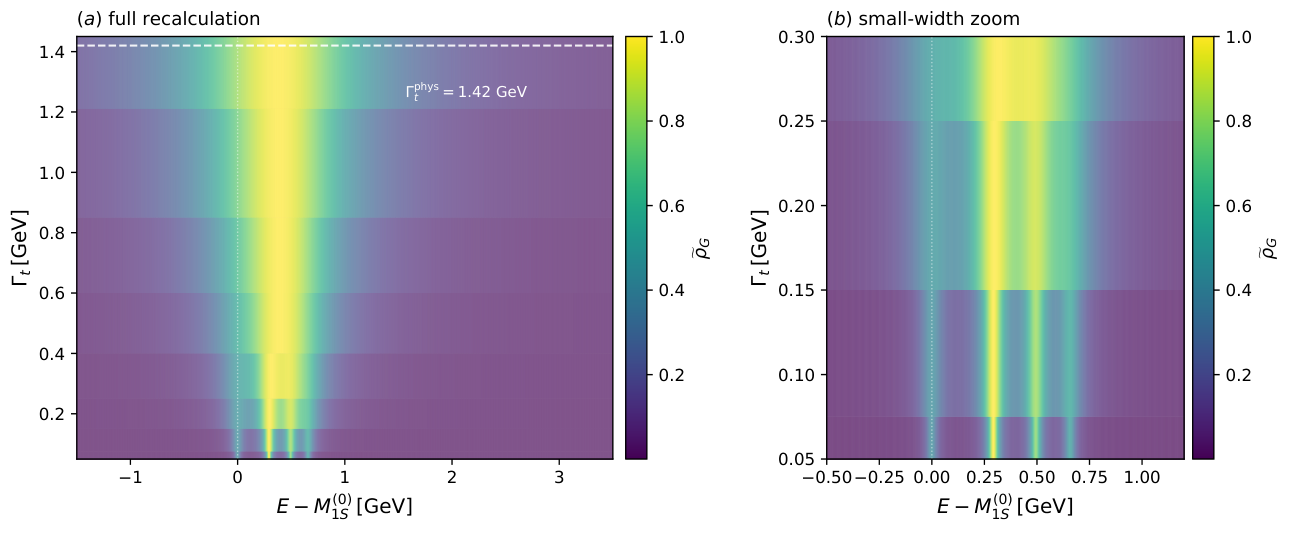
The title of this work emphasizes the loss of radial resolvability as the inherited top width increases. To establish that this loss is not a frozen-residue artifact, we perform a full width-dependent non-Hermitian re-diagonalization: for each value of $\Gamma_{t}$ the Salpeter operator $H(m_{t}-i\Gamma_{t}/2)$ is reconstructed from scratch and the biorthogonal eigenproblem is solved anew, giving $\mathcal{M}_{n}(\Gamma_{t})$, $L_{n}(\Gamma_{t})$, $R_{n}(\Gamma_{t})$, and the raw residues $Z_{n}^{\rm raw}(\Gamma_{t})$. The full-recalculation response is

$$\rho_{G}(E;\Gamma_{t})=-\frac{1}{\pi}\operatorname{Im}\sum_{n=1}^{4}\frac{Z_{n}^{\rm raw}(\Gamma_{t})}{E-\mathcal{M}_{n}(\Gamma_{t})}.$$

(34)

The state tracking across widths uses the biorthogonal overlap $\mathcal{O}_{mn}=|L_{m}^{\dagger}(\Gamma_{i})R_{n}(\Gamma_{i+1})|$, with greedy maximum-overlap assignment; the resulting assignment is the identity across all transitions, with maximum off-diagonal overlap below $4\times 10^{-5}$ for all three channels.

For direct comparison we also retain the leading heavy-top-limit frozen-residue approximation,

$$\rho_{\rm frozen}(E;\Gamma_{t})=-\frac{1}{\pi}\operatorname{Im}\sum_{n=1}^{4}\frac{Z_{n}^{\rm raw}(\Gamma_{t}^{\rm phys})}{E-M_{n}^{(0)}+i\Gamma_{t}/2},$$

(35)

which fixes the real pole positions at the stable-limit values $M_{n}^{(0)}$, sets $\Gamma_{n}=\Gamma_{t}$, and freezes the residues at their physical-width values. The frozen-residue scan captures the qualitative dissolution pattern, while the full non-Hermitian evolution modifies the intermediate-width crossover quantitatively; both prescriptions agree that the physical-width response has a single broad maximum.

The scan is performed at $\Gamma_{t}=0$, $0.05$, $0.10$, $0.20$, $0.30$, $0.50$, $0.70$, $1.00$, and $1.42$ GeV (Table 6). For the heatmap, $\Gamma_{t}$ is sampled at $N_{\Gamma}=50$ uniformly spaced points between $0.05$ and $1.42$ GeV. Only the four lowest radial poles are retained, so that the figure isolates the resolvability of the $1S$–$4S$ pattern without incorporating additional discretized-basis eigenmodes. The $\Gamma_{t}=0$ limit is excluded from the heatmap because the Lorentzian peaks approach delta distributions whose sampled heights become grid dependent. For visualization, each response is normalized to its own maximum,

$$\widetilde{\rho}_{G}(E;\Gamma_{t})=\frac{\rho_{G}(E;\Gamma_{t})}{\max_{E}\rho_{G}(E;\Gamma_{t})}.$$

(36)

Each curve is normalized to its own maximum for visualization, so that the narrow small-width peaks do not compress the physical-width response. This normalization removes the absolute response strength and is used only to compare the number and locations of resolvable maxima.

The peak count is determined with scipy.signal.find_peaks, using a relative prominence threshold of $5\%$ of the curve maximum and a minimum separation of five grid points. Table 6 reports the peak count for the full-recalculation response $\rho_{G}(E;\Gamma_{t})$ of Eq. (34). In the $t\bar{b}$ channel, four resolved maxima remain visible up to $\Gamma_{t}=0.10$ GeV. At $\Gamma_{t}=0.20$ GeV, the weakest $4S$ feature falls below the operational prominence threshold, so the four-peak pattern is no longer fully resolvable. By $\Gamma_{t}\geq 0.30$ GeV, only one maximum remains. The $t\bar{c}$ channel shows the same progression (four peaks at $\Gamma_{t}\leq 0.05$ GeV, three at $0.10$ GeV, two at $0.20$–$0.30$ GeV, one at $\Gamma_{t}\geq 0.50$ GeV). The $t\bar{u}$ channel shows only two resolvable peaks at small width because the $1S$ residue is $77.8\%$ of the sum, so the $3S$ and $4S$ features are too weak to register as separate maxima under the $5\%$ prominence threshold; the $2S$ feature is clearly visible and merges with $1S$ by $\Gamma_{t}=0.20$ GeV. The peak count is operational and should not be interpreted as a universal experimental boundary. The channel-dependent peak count at small width illustrates that, at the quantitative level, the resolvability criterion is source-dependent; however, the physical-width single-broad-maximum conclusion is robust across all channels and source variations.

Crucially, the real pole positions move by less than $1.4\times 10^{-7}$ GeV across the entire scan, far smaller than $\Gamma_{t}$ itself, and the ratio $\Gamma_{n}/\Gamma_{t}$ at the physical width is $0.99995$–$1.00000$ for all four radial states and all three channels (Table 9). The simple heavy-top-limit width inheritance $\Gamma_{n}\simeq\Gamma_{t}$ is therefore quantitatively validated by the full non-Hermitian re-diagonalization.

Together with the source-parameter tests in Sec. IV.5, this full evolution illustrates how the hierarchy $\Gamma_{t}\gg\Delta M$ removes the resolvability of the four-pole pattern, and confirms that the conclusion does not rely on a frozen-residue approximation.

The single-maximum conclusion at the physical width is unchanged under variations of the Gaussian source width $\beta$ (scanned at $0.3$, $0.5$, $0.8$, $1.0$ GeV) and the component-weight ratio $c_{2}/c_{1}$ (scanned at $0$, $0.5$, $1$, $2$). The random positive-residue scan described in Appendix B now plays an auxiliary role: with the pole-sector source-projected response in hand, the positive-residue scan is no longer a core piece of evidence but a robustness check on the normalized positive diagnostic. Detailed residue tables and peak-count tests are collected in Appendix A and Appendix B.

Resolving two levels separated by $\Delta M$ requires coherence over a time of order $t_{\rm res}\sim 1/\Delta M$. The probability that the top survives weak decay over that interval is

$$P_{\rm surv}(t_{\rm res})\simeq\exp(-\Gamma_{t}t_{\rm res})=\exp\!\left(-\frac{\Gamma_{t}}{\Delta M}\right)\simeq\exp\!\left(-\frac{1}{\mathcal{R}}\right).$$

(37)

For the first radial splitting, Table 3 gives a survival factor of order $10^{-2}$. The definition $t_{\rm res}\sim 1/\Delta M$ carries an order-one convention dependence; the individual percentages are not precision predictions. Equation (37) is a timescale estimate rather than a top-meson formation probability.

References

- [1] (2025) Observation of a pseudoscalar excess at the top quark pair production threshold. Rept. Prog. Phys. 88 (8), pp. 087801. External Links: 2503.22382, Document Cited by: §I.
- [2] (2026) Observation of a cross-section enhancement near the production threshold in TeV collisions with the ATLAS detector. Rept. Prog. Phys. 89 (5), pp. 057801. External Links: 2601.11780, Document Cited by: §I.
- [3] (2025) Third-order correction to top-quark pair production near threshold. Part I. Effective theory set-up and matching coefficients. JHEP 07, pp. 273. External Links: 1312.4791, Document Cited by: §I.
- [4] (2025) Third-order correction to top-quark pair production near threshold II. Potential contributions. JHEP 07, pp. 274. External Links: 2409.05960, Document Cited by: §I.
- [5] (2025) Updated predictions for toponium production at the LHC. Phys. Lett. B 866, pp. 139532. External Links: 2412.16685, Document Cited by: §I.
- [6] (2025) Analytic NNLO transverse-momentum-dependent soft function for heavy quark pair hadroproduction at threshold. JHEP 10, pp. 164. External Links: 2506.23791, Document Cited by: §I, §I.
- [7] (2021) Signatures of toponium formation in LHC run 2 data. Phys. Rev. D 104 (3), pp. 034023. External Links: 2102.11281, Document Cited by: §I.
- [8] (2025) Simulating toponium formation signals at the LHC. Eur. Phys. J. C 85 (2), pp. 157. External Links: 2411.18962, Document Cited by: §I.
- [9] (2024) Toponium hunter’s guide. Phys. Rev. D 110 (5), pp. 054032. External Links: 2407.20330, Document Cited by: §I, §I.
- [10] (2025) QCD Sum Rule Study of Topped Mesons Within Heavy Quark Effective Theory. Universe 11 (10), pp. 334. External Links: 2508.03422, Document Cited by: §I, §I.
- [11] (2025) Topped baryons from QCD sum rules. arXiv preprint arXiv:2507.05895. External Links: 2507.05895 Cited by: §I.
- [12] (2025) The quest for topped hadrons. arXiv preprint arXiv:2508.17646. External Links: 2508.17646 Cited by: §I.
- [13] (2026) The S-wave topped meson. Chin. Phys. C 50 (9), pp. 093108. External Links: 2602.09684, Document Cited by: §I, §I, §I, §II.1, §II.3.
- [14] (2026) Top-quark mass interpretation from simulation of top-flavoured mesons. arXiv:2607.24935. External Links: 2607.24935 Cited by: §I.
- [15] (1998) Top mesons. Eur. Phys. J. C 2, pp. 345–350. External Links: hep-ph/9704261, Document Cited by: §I.
- [16] (1986) Production and Decay Properties of Ultraheavy Quarks. Phys. Lett. B 181, pp. 157–163. External Links: Document Cited by: §I, §I.
- [17] (2024) Review of particle physics. Phys. Rev. D 110 (3), pp. 030001. External Links: Document Cited by: §I.
- [18] (2026) Toponium Spectrum in the Complex-Energy Plane. arXiv:2607.14554. External Links: 2607.14554 Cited by: §I, §V.
- [19] (2026) Top-Antitop Production and Decay at Threshold at the LHC in QCD Perturbation Theory. arXiv:2607.09539. External Links: 2607.09539 Cited by: §I, §II.4, §V.
- [20] (2025) Mass spectra and wave functions of toponia. Phys. Rev. D 111 (9), pp. 096016. External Links: 2411.17955, Document Cited by: §I.
- [21] (2025) Toponium: The smallest bound state and simplest hadron in quantum mechanics. Phys. Rev. D 111 (11), pp. 114020. External Links: 2412.11254, Document Cited by: §I.
- [22] (2025) Ensuring that toponium is glued, not nailed. Phys. Lett. B 866, pp. 139510. External Links: 2411.19180, Document Cited by: §I.
- [23] (2025) Spin correlations in production and decay at the LHC in QCD perturbation theory. JHEP 10, pp. 149. External Links: 2505.00096, Document Cited by: §I.
- [24] (1951) A Relativistic Equation for Bound-State Problems. Phys. Rev. 82, pp. 309–310. External Links: Document Cited by: §II.1.
- [25] (1996) Possible retardation effects of quark confinement on the meson spectrum. Phys. Rev. D 54, pp. 2273–2278. External Links: hep-ph/9603274, Document Cited by: §II.1, §II.3.
- [26] (2006) Decay constants of heavy vector mesons in relativistic Bethe-Salpeter method. Phys. Lett. B 633, pp. 492–496. External Links: math-ph/0512009, Document Cited by: §II.1.
- [27] (2004) Decay constants of heavy meson of 0- state in relativistic Salpeter method. Phys. Lett. B 596, pp. 84–89. External Links: hep-ph/0405112, Document Cited by: §II.1.
- [28] (1978) Charmonium: Comparison with experiment. Phys. Rev. D 17, pp. 3090. External Links: Document Cited by: §II.3.
- [29] (1984) The Heavy Quark Potential in SU(3) Lattice Gauge Theory. Phys. Rev. D 29, pp. 1213. External Links: Document Cited by: §II.3.
- [30] (1984) SU (3) Heavy-Quark Potential with High Statistics. Phys. Rev. Lett. 53, pp. 1028–1028. External Links: Document Cited by: §II.3.
- [31] (1984) The Force Between Static Quarks. Phys. Rev. D 30, pp. 1293. External Links: Document Cited by: §II.3.
- [32] (1987) Spin Spin and Spin - Orbit Potentials From Lattice Gauge Theory. Nucl. Phys. B 286, pp. 211–230. External Links: Document Cited by: §II.3.
- [33] (1986) The Long Range Spin Orbit Potential. Phys. Rev. Lett. 56, pp. 1219. External Links: Document Cited by: §II.3.
- [34] (1986) The Interquark Potential: SU(2) Color Gauge Theory With Fermions. Phys. Lett. B 173, pp. 437–442. External Links: Document Cited by: §II.3.
- [35] (2006) The Complex-mass scheme for perturbative calculations with unstable particles. Nucl. Phys. B Proc. Suppl. 160, pp. 22–26. External Links: hep-ph/0605312, Document Cited by: §II.4.
- [36] (2005) Spectra and pseudospectra: the behavior of nonnormal matrices and operators. Princeton University Press, Princeton. Cited by: §II.5.
- [37] (2024) Hellmann-Feynman theorem in non-Hermitian systems. Phys. Rev. A 109 (2), pp. 022227. External Links: Document Cited by: §II.5.