The method of ellipcenters with momentum and relaxation for convex quadratic minimization

Roger Behling

Department of Mathematics, UFSC

Blumenau, Santa Catarina, Brazil

rogerbehling@gmail.com

Vincent Guigues

School of Applied Mathematics, FGV

Praia de Botafogo, Rio de Janeiro, Brazil

vincent.guigues@fgv.br

Harry Oviedo

Department of Mathematics

Instituto Tecnológico Autónomo de México, ITAM

Mexico city, Mexico

harry.oviedo@uai.cl

Abstract. The method of ellipcenters (ME) is a recent technique developed for unconstrained minimization. Its iteration relies only on first order information and consists of building a suitable two-dimensional ellipse that tries to capture intrinsic ill-conditioning of the problem. The center of the ellipse is taken as the next iterate, which justifies the name of the method. ME was already shown to converge linearly when the objective function is smooth and strongly convex. The special case when the objective is quadratic was studied in the first paper on ME and is also the subject of our work here. In this paper, we propose two variants of ME: RelaxME which adds in ME an additional relaxation step at each iteration and MomME which embeds momentum in ME. We prove linear convergence of RelaxME and MomME and, in particular, we show convergence of RelaxME and MomME (and also of ME) in one iteration when the matrix of the quadratic form has only two distinct eigenvalues. Finally, we provide the results of numerical experiments which compare on five optimization problems (and different combinations of parameters defining these problems) ME, RelaxME, and MomME, with 3 other optimizers: the conjugate gradient method [10], Barzilai and Borwein gradient method with long step [2], and the gradient method with adaptive spectral step length [7]. On most instances, MomME provides the smallest number of iterations and conjugate gradient and MomME provide the smallest CPU times and similar CPU times. This opens optimistic possibilities for ME with momentum in broader settings.

Keywords. Quadratic optimization, ellipcenter, relaxation, optimization method with momentum, finite convergence, image smoothing.

1 Introduction

We present two procedures (relaxation and momentum) in order to accelerate the Method of Ellipcenters (ME), a recent first order technique that employs centers of suitable two-dimensional ellipses for minimizing a strongly convex and differentiable function $f:\mathbb{R}^{n}\rightarrow\mathbb{R}$ . ME iterates by moving from a current iterate $x_{k}\in\mathbb{R}^{n}$ to a point $x_{k+1}\in\mathbb{R}^{n}$ that is the center of a special ellipse $E_{k}$ .

Let us start by describing ME formally as it was introduced in [4]. Consider that $x_{k}\in\mathbb{R}^{n}$ is the current iterate of ME. If it is stationary, that is, $\nabla f(x_{k})=0$ , we are already at the unique minimizer of $f$ and ME stops with success. When $x_{k}$ is non-stationary, ME computes the unique point $y_{k}\neq x_{k}$ such that $y_{k}=x_{k}-t_{k}\nabla f(x_{k})$ and $f(y_{k})=f(x_{k})$ . Then, if $\mbox{span}\{\nabla f(x_{k}),\nabla f(y_{k})\}$ is one-dimensional, ME returns $(x_{k}+y_{k})/2$ . If $\nabla f(x_{k})$ and $\nabla f(y_{k})$ are linearly independent, ME takes the next iterate as the center of an ellipse $E_{k}$ fulfilling the following three properties:

ME1

$E_{k}$ is an ellipse contained in

\Pi_{k}:=\Big\{x\in\mathbb{R}^{n}:x=x_{k}+\mbox{span}\{\nabla f(x_{k}),\nabla f(y_{k})\}\Big\};

(1)

ME2

$E_{k}$ is orthogonal to $\nabla f(x_{k})$ at $x_{k}$ ;

ME3

$E_{k}$ is orthogonal to $\nabla f(y_{k})$ at $y_{k}$ .

The intention of ME is to capture ill-conditioning through two-dimensional elliptical interpolations. Its geometry is illustraded in Figure 1.

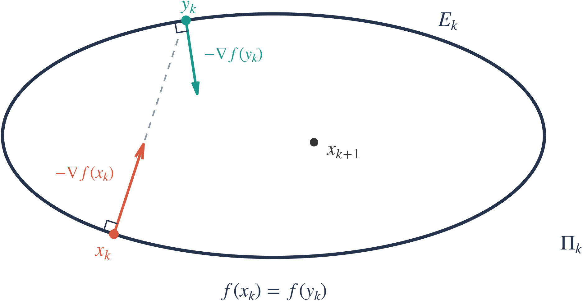
Refer to caption — Figure 1: Illustration of an iteration of ME.

The construction of an ellipse, i.e., a two-dimensional ellipsoid is not in vain. There are several reasons for that. One is that the zigzagging of the Cauchy method (steepest descent with optimal line-search) for a strictly convex quadratic objective gets, in the limit, smashed into a two-dimensional affine space related to the two extreme eigenvalues of the Hessian (see [1], [14], and [9]). Moreover, level sets of strictly convex quadratics are ellipsoids which, in turn, provide good approximations of level sets of a wide range of smooth convex functions. So ME is somewhat designed to encage the minimizer by ellipsoids constrained to the two-dimensional affine spaces $\Pi_{k}$ described above. For a strictly convex quadratic in $\mathbb{R}^{2}$ , ME fences in the minimizer perfectly and yields finite convergence in one single step. In particular, it coincides with Newton’s method in this simple context.

Very recently, ME has been studied for strongly convex minimization. In [3], the set of ellipses and associated centers has been characterized using standard Analytic Geometry. It turns out that there is an infinite number of ellipses satisfying ME1, ME2, and ME3. Furthermore, the correspondent centers lie in an appropriate half-line starting at $\frac{1}{2}(x_{k}+y_{k})$ and going in a certain direction $d_{k}$ , that depends on $x_{k},y_{k}$ and their gradients with respect to $f$ (see the formula in [3]). The starting point $\frac{1}{2}(x_{k}+y_{k})$ is somewhat degenerate, as the associated ”ellipse” becomes simply the segment with end points $x_{k}$ and $y_{k}$ . One can then, among all ellipcenters, look for the point $x_{k+1}$ that minimizes $f$ along this half-line $S_{k}:=\{x\in\mathbb{R}^{n}:x=\frac{1}{2}(x_{k}+y_{k})+td_{k},\mbox{ }t\geq 0\}$ of centers of ellipses. This particular center of ellipse given by the minimizer of $f$ in $S_{k}$ will be referred to as the best ellipcenter with respect to $x_{k}$ and denoted by $\mbox{ME}(x_{k})$ . It was shown in [3] that, by defining ME in this way, the method achieves linear convergence to the unique global minimizer of the smooth strongly convex objective $f$ .

As said earlier, this work will focus on $f$ being not only strongly convex and differentiable, but also quadratic. That said, it will not be necessary for us to go further into details on the construction of the half-line of ellipcenters $S_{k}$ . We can avoid this discussion, because the best ellipcenter $\mbox{ME}(x_{k})$ happens to be the minimizar of $f$ in the plane $\Pi_{k}$ when $f$ is quadratic, see [4], and thus $\mbox{ME}(x_{k})$ is essentially provided by the outcome of a simple $2\times 2$ linear system of equations. We observe that this characterization of $\mbox{ME}(x_{k})$ being the minimizer of $f$ in $\Pi_{k}$ is no longer true for general smooth strongly convex minimization, see the discussion in [3] and how it implies that the method in [5] is different from ME.

For the rest of the paper, we consider optimization methods to solve the problem

\min_{x\in\mathbb{R}^{n}}f(x):=\frac{1}{2}x^{T}Ax-b^{T}x+c

(2)

where is $f$ a strongly convex quadratic function, i.e., $A\in\mathbb{R}^{n\times n}$ is a symmetric positive definite matrix, $b\in\mathbb{R}^{n}$ , and $c$ is a scalar. We will denote by $x_{*}$ the optimal solution of (2).

We now list the three main contributions of our paper. The first one regards the improvement on the rate of convergence of ME itself. In [4], it was shown that ME, for minimizing the quadratic $f$ , has a convergence rate better or equal to $\eta$ , where $\eta$ is the linear rate for the Cauchy method. We show that, actually, the rate of ME is at least as good as the rate provided by two successive Cauchy steps, that is, ME converges with rate $\eta^{2}$ . Our second contribution consists of considering in ME the general relaxation framework by [17]. We call RelaxME the corresponding variant of ME. We prove that RelaxME also enjoys linear convergence and shares the same theoretical linear rate $\eta^{2}$ of ME for the case when the relaxation parameter is $1$ . In our experiments, however, RelaxME consistently outperforms ME. Finally, we employ Nesterov’s momentum [12] within ME, getting what we call MomME. MomME still maintains the rate $\eta^{2}$ in theory, but behaves way faster than both ME and RelaxME, in practice. Moreover, we prove finite convergence of ME, RelaxME, and MomME when $A$ has at most two different eigenvalues.

Before moving on with the presentation of the organization of the paper, let us briefly point out some facts that may already help with the understanding of the sections ahead. We note that $f$ being a strictly convex quadratic gives us some nice properties. Indeed, it turns out that the Cauchy point computed at the non-stationary iterate $x_{k}$ , denoted here by $\mbox{Cauchy}(x_{k})$ is simply given by $\frac{1}{2}(x_{k}+y_{k})$ , with $y_{k}$ being the auxiliary point defined in ME. More than that, $\nabla f(\mbox{Cauchy}(x_{k}))=A(\frac{1}{2}(x_{k}+y_{k}))-b=\frac{1}{2}\nabla f(x_{k})+\frac{1}{2}\nabla f(y_{k})$ . This means, in particular, that $\nabla f(\mbox{Cauchy}(x_{k}))\in\mbox{span}\{\nabla f(x_{k}),\nabla f(y_{k})\}$ . Also, one can prove that if $\nabla f(x_{k})$ and $\nabla f(y_{k})$ are linearly dependent, $\nabla f(\mbox{Cauchy}(x_{k}))=0$ and ME (and also RelaxME and MomME) is done with the minimization of $f$ , see Lemma 2.2 below. Finally, when $\mbox{span}\{\nabla f(x_{k}),\nabla f(y_{k})\}$ is two-dimensional, it follows trivially from our observations that $\mbox{Cauchy}(\mbox{Cauchy}(x_{k}))\in\Pi_{k}$ . However, recall that $x_{k+1}:=\mbox{ME}(x_{k})$ is the minimizer of $f$ in $\Pi_{k}$ now that $f$ is quadratic. Long story short, we are saying that one iteration of ME is better or equal, by means of function value, than two consecutive steps of the Cauchy method. This is the main reason for us to get the rate $\eta^{2}$ mentioned above.

Our paper is organized as follows. In Section 2, we describe RelaxME, show several properties of this method, and show its convergence. In Section 3, we describe the variant MomME of ME and prove its convergence. In Section 4, we prove the convergence of ME, RelaxME, and MomME in one iteration when $A$ has at most two different eigenvalues. Finally, in Section 5, we provide the results of numerical experiments which compare on five optimization problems (and different combinations of parameters defining these problems) ME, RelaxME, MomME, with 3 other optimizers: the conjugate gradient method [10], Barzilai and Borwein gradient method with long step [2], and the gradient method with adaptive spectral step length [7]. In most instances, MomME provides the smallest number of iterations and conjugate gradient and MomME provide the smallest CPU times and similar CPU times. This opens optimistic possibilities for ME with momentum in broader settings.

Notation and terminology

For $x\in\mathbb{R}^{n}$ , and $A$ an $n\times n$ definite positive matrix, we denote by $\|\cdot\|_{A}$ the norm defined by

\|x\|_{A}=\sqrt{x^{T}Ax}

induced by the scalar product $\langle x,y\rangle_{A}=x^{T}Ay$ for $x,y\in\mathbb{R}^{n}$ . Given an $n\times n$ definite positive matrix $A$ , we say that vectors $x,y\in\mathbb{R}^{n}$ are $A$ -conjugate if $\langle x,y\rangle_{A}=0$ .

For vectors $x,y\in\mathbb{R}^{n}$ , we will use the notation $\langle x,y\rangle$ for the scalar product $x^{T}y$ with corresponding norm $\|\cdot\|$ .

2 RelaxME

2.1 Motivation and algorithm

In this subsection, we introduce and analyze the convergence of the relaxed variant RelaxME of ME. More precisely, at a given iteration where $x_{k}$ was the last point computed by RelaxME (the point computed in the previous iteration), we first compute $\tilde{x}_{k+1}$ performing one iteration of ME. Given a relaxation parameter $\theta\in(0,1]$ , we then compute the next iterate $x_{k+1}$ as the convex combination $x_{k+1}=(1-\theta)x_{k}+\theta\tilde{x}_{k+1}$ between the previous iterate $x_{k}$ and $\tilde{x}_{k+1}$ . We recall that given $x_{k}$ such that $\nabla f(x_{k})\neq 0$ , an iteration of ME first computes $y_{k}=x_{k}-t_{k}\nabla f(x_{k})$ such that $f(y_{k})=f(x_{k})$ . If $\nabla f(y_{k})$ and $\nabla f(x_{k})$ are linearly independent, then $\tilde{x}_{k+1}$ minimizes $f$ in the affine space $x_{k}+\mbox{Span}(\nabla f(x_{k}),\nabla f(y_{k}))$ . It is worth mentioning that the minimizer $x_{k}+\alpha_{k}\nabla f(x_{k})+\beta_{k}\nabla f(y_{k})$ of $f$ in this affine space is known in analytic form. If $\nabla f(y_{k})$ and $\nabla f(x_{k})$ are linearly dependent, then $\tilde{x}_{k+1}=(1/2)(x_{k}+y_{k})$ . The statement of Relaxed ME is given in Algorithm 1. As shown in [4], the formula given for $t_{k}$ in this algorithm ensures that $f(y_{k})=f(x_{k})$ . Moreover, as shown in Lemma 2.1, the sequences $(g_{k})$ and $(r_{k})$ computed iteratively satisfy $g_{k}=\nabla f(x_{k})$ and $r_{k}=\nabla f(y_{k})$ for all $k\geq 0$ .

Algorithm 1 Relaxed Method of Ellipcenters for Convex Quadratic Minimization (RelaxME)

1: Initialization.

2: Let

A\in\mathbb{R}^{n\times n}

be symmetric positive definite,

b\in\mathbb{R}^{n}

, and

x_{0}\in\mathbb{R}^{n}

3: Set

\widetilde{x}_{0}=x_{0},\qquad g_{0}=\nabla f(x_{0}),\qquad\theta\in(0,1],\qquad k=0.

4: while

\lVert g_{k}\rVert\geq\varepsilon

w_{k}=Ag_{k}

\displaystyle t_{k}=\frac{2\lVert g_{k}\rVert^{2}}{g_{k}^{\top}w_{k}}

y_{k}=x_{k}-t_{k}g_{k}

r_{k}=g_{k}-t_{k}w_{k}

9: if

g_{k}

and

r_{k}

are linearly independent then

10:

\displaystyle(\alpha_{k},\beta_{k})=\operatorname*{arg\,min}_{\alpha,\beta}f\bigl(x_{k}+\alpha g_{k}+\beta r_{k}\bigr)

11:

\widetilde{x}_{k+1}=x_{k}+\alpha_{k}g_{k}+\beta_{k}r_{k}

12: else

13:

\displaystyle\widetilde{x}_{k+1}=\frac{1}{2}(x_{k}+y_{k})

14:

x_{k+1}=\widetilde{x}_{k+1}

15:

g_{k+1}=\nabla f(\widetilde{x}_{k+1})

16: break

17: end if

18: if

k=0

then

19:

x_{k+1}=\widetilde{x}_{k+1}

20:

g_{k+1}=\nabla f(\widetilde{x}_{k+1})

21: else

22:

x_{k+1}=(1-\theta)x_{k}+\theta\widetilde{x}_{k+1}

23:

g_{k+1}=(1-\theta)g_{k}+\theta\nabla f(\widetilde{x}_{k+1})

24: end if

25:

k=k+1

26: end while

In the next subsection, we prove several properties of RelaxME.

2.2 Properties of RelaxME

In the following lemma, we show that for every $k\geq 0$ , $g_{k}$ is the gradient of $f$ at $x_{k}$ and $r_{k}$ is the gradient of $f$ at $y_{k}$ .

Lemma 2.1.

For every $k\geq 0$ , we have $g_{k}=\nabla f(x_{k})$ and $r_{k}=\nabla f(y_{k})$ .

Proof: The proof is by induction on $k$ . For $k=0$ , the initialization step of the algorithm gives $g_{0}=\nabla f(x_{0})$ and for $k=1$ the algorithm computes $g_{1}=\nabla f(x_{1})$ . Now assume that for $k\geq 1$ we have $g_{k}=\nabla f(x_{k})$ . We want to show that $g_{k+1}=\nabla f(x_{k+1})$ . At iteration $k+1$ , if the algorithm stops at the break command at line 15, we have $g_{k+1}=\nabla f(x_{k+1})$ by definition of $g_{k+1}$ . Otherwise, we have ${x}_{k+1}=(1-\theta)x_{k}+\theta{\tilde{x}}_{k+1}$ , which implies

$\displaystyle\nabla f(x_{k+1})$	$\displaystyle=$	$\displaystyle Ax_{k+1}-b$	(3)
	$\displaystyle=$	$\displaystyle A\Big((1-\theta)x_{k}+\theta{\tilde{x}}_{k+1}\Big)-b$
	$\displaystyle=$	$\displaystyle(1-\theta)(Ax_{k}-b)+\theta(A\tilde{x}_{k+1}-b)$
	$\displaystyle=$	$\displaystyle(1-\theta)\nabla f(x_{k})+\theta(A\tilde{x}_{k+1}-b)$
	$\displaystyle=$	$\displaystyle(1-\theta)g_{k}+\theta\nabla f(\tilde{x}_{k+1})\;\;\mbox{ (by the induction assumption)}$
	$\displaystyle=$	$\displaystyle g_{k+1}\;\;\mbox{(by definition of $g_{k+1}$)}$

which shows the relation $g_{k}=\nabla f(x_{k})$ for all $k\geq 0$ . Finally,

r_{k}=g_{k}-t_{k}w_{k}=\nabla f(x_{k})-t_{k}Ag_{k}=Ax_{k}-b-t_{k}Ag_{k}=Ay_{k}-b=\nabla f(y_{k}),

which achieves the proof of the lemma.

Observe that the condition $g_{k}=\nabla f(x_{k})$ and $r_{k}=\nabla f(y_{k})$ linearly dependent can be written $\|\nabla f(x_{k})\|=\|\nabla f(y_{k})\|$ . Indeed, it is easy to check that $\langle\nabla f(x_{k}),\nabla f(y_{k})\rangle=-\|\nabla f(x_{k})\|^{2}$ and vectors $g_{k}$ and $r_{k}$ are linearly dependent if and only if $|\cos(\angle(\nabla f(x_{k}),\nabla f(y_{k})))|=1$ which can be written equivalently

1=\left|\frac{\langle\nabla f(x_{k}),\nabla f(y_{k})\rangle}{\|\nabla f(x_{k})\|\|\nabla f(y_{k})\|}\right|=\frac{\|\nabla f(x_{k})\|}{\|\nabla f(y_{k})\|}.

We now introduce error terms

e_{k}=x_{k}-x_{*}\mbox{ and }\tilde{e}_{k}=\tilde{x}_{k}-x_{*}

(4)

that will be useful in our analysis as well as

d_{k}=e_{k}-\tilde{e}_{k+1}.

(5)

Another interesting property of RelaxME, shown in the following lemma, is that if at a given iteration $k$ , vectors $g_{k}$ and $r_{k}$ are linearly dependent then this is the last iteration of the method which outputs the optimal solution $x_{*}$ . This justifies the break command at line 15 of the algorithm.

Lemma 2.2.

If $g_{k}$ and $r_{k}$ are linearly dependent we have $x_{k+1}=\tilde{x}_{k+1}=x_{*}$ , i.e., RelaxME has computed the minimum of $f$ in a finite number of iterations.

Proof: If $g_{k}$ and $r_{k}$ are linearly dependent, there is $\lambda$ such that $Ag_{k}=\lambda g_{k}$ . Therefore $\lambda>0$ is eigenvalue and $g_{k}$ eigenvector of $A$ . It follows that

t_{k}=\frac{2\|g_{k}\|^{2}}{g_{k}^{T}Ag_{k}}=\frac{2}{\lambda}

and from the iterations of the method, we have

\tilde{x}_{k+1}=\frac{1}{2}(x_{k}+y_{k})=x_{k}-\frac{t_{k}}{2}g_{k}=x_{k}-\frac{1}{\lambda}g_{k}.

(6)

Since $Ax_{*}=b$ , we then have

Ae_{k}\stackrel{{\scriptstyle\eqref{defeketk}}}{{=}}A(x_{k}-x_{*})=Ax_{k}-b=\nabla f(x_{k})=g_{k}

(7)

where the last equality comes from Lemma 2.1. Therefore we have

e_{k}=A^{-1}g_{k}=\frac{1}{\lambda}g_{k}

(8)

and

x_{k+1}=\tilde{x}_{k+1}\stackrel{{\scriptstyle\eqref{ekfc0},\eqref{ekfc1}}}{{=}}x_{k}-e_{k}\stackrel{{\scriptstyle\eqref{defeketk}}}{{=}}x_{*}.

(9)

The following lemma provides additional insights on RelaxME which are useful for its convergence analysis.

Lemma 2.3.

The following holds for error terms $(e_{k})$ , $(\tilde{e}_{k})$ , and sequence $(d_{k})$ : for every $k\geq 0$ such that $g_{k}$ and $r_{k}$ are linearly independent,

(A)

$d_{k}$ and $\tilde{e}_{k+1}$ are $A$ -conjugate;
(B)

we have

$\|e_{k}\|_{A}^{2}=\|\tilde{e}_{k+1}\|_{A}^{2}+\|d_{k}\|_{A}^{2};$ (10)
(C)

we have

$\|e_{k+1}\|_{A}^{2}=\|\tilde{e}_{k+1}\|_{A}^{2}+(1-\theta)^{2}\|d_{k}\|_{A}^{2}.$ (11)

Proof: (A) Observe that if $g_{k}$ and $r_{k}$ are linearly independent,

d_{k}=x_{k}-\tilde{x}_{k+1}\in\mbox{Span}(g_{k},r_{k}).

(12)

Next, by the optimality conditions for the problem solved in the linearly independent case,

\langle\nabla f(\tilde{x}_{k+1}),g_{k}\rangle=0\mbox{ and }\langle\nabla f(\tilde{x}_{k+1}),r_{k}\rangle=0

which implies

\nabla f(\tilde{x}_{k+1})\in\mbox{Span}(g_{k},r_{k})^{\perp}.

(13)

Combining (12) and (13), we obtain

0=d_{k}^{T}\nabla f(\tilde{x}_{k+1})=d_{k}^{T}[A\tilde{x}_{k+1}-b]=d_{k}^{T}A\tilde{e}_{k+1}=\langle d_{k},\tilde{e}_{k+1}\rangle_{A},

(14)

which achieves the proof of (A).

(B) We deduce from (A) that

$\displaystyle\\|e_{k}\\|_{A}^{2}$	$\displaystyle=$	$\displaystyle\\|\tilde{e}_{k+1}+d_{k}\\|_{A}^{2}$	(15)
	$\displaystyle=$	$\displaystyle\\|\tilde{e}_{k+1}\\|_{A}^{2}+\\|d_{k}\\|_{A}^{2}+2\langle d_{k},\tilde{e}_{k+1}\rangle_{A}$
	$\displaystyle\stackrel{{\scriptstyle\eqref{span3}}}{{=}}$	$\displaystyle\\|\tilde{e}_{k+1}\\|_{A}^{2}+\\|d_{k}\\|_{A}^{2},$

which proves (10).

$\displaystyle e_{k+1}$	$\displaystyle=$	$\displaystyle x_{k+1}-x_{*}$	(16)
	$\displaystyle=$	$\displaystyle(1-\theta)x_{k}+\theta\tilde{x}_{k+1}-x_{*}$
	$\displaystyle=$	$\displaystyle(1-\theta)(x_{k}-x_{})+\theta(\tilde{x}_{k+1}-x_{})$
	$\displaystyle=$	$\displaystyle(1-\theta)e_{k}+\theta\tilde{e}_{k+1}$
	$\displaystyle=$	$\displaystyle(1-\theta)({\tilde{e}}_{k+1}+d_{k})+\theta\tilde{e}_{k+1}$
	$\displaystyle=$	$\displaystyle\tilde{e}_{k+1}+(1-\theta)d_{k}.$

Using (14), (16), and the Pythagorean theorem, we have

\|e_{k+1}\|_{A}^{2}=\|\tilde{e}_{k+1}\|_{A}^{2}+(1-\theta)^{2}\|d_{k}\|_{A}^{2},

(17)

which achieves the proof of (11).

In what follows we denote by $0<\lambda_{1}\leq\lambda_{2}\leq\ldots\leq\lambda_{n}$ the eigenvalues of matrix $A$ .

The following lemma will be useful for the convergence analysis of RelaxME, shown in Section 2.3.

Lemma 2.4.

For every $k\geq 0$ , we have

f(\tilde{x}_{k+1})-f(x_{*})\leq\rho^{4}(f(x_{k})-f(x_{*}))

(18)

where

\rho=\frac{\kappa-1}{\kappa+1}\mbox{ with }\kappa=\frac{\lambda_{n}}{\lambda_{1}}.

(19)

Proof: We consider two cases: the case where $g_{k}$ and $r_{k}$ are linearly independent and the case where they are linearly dependent.

Case where $g_{k}$ and $r_{k}$ are linearly independent.¹¹ 1 The reader can find a second proof of (18) in this case in the Appendix.

In this case, $\tilde{x}_{k+1}\in x_{k}+\mbox{Span}(g_{k},r_{k})$ . Since $r_{k}=g_{k}-t_{k}Ag_{k}$ with $t_{k}>0$ , we have $\mbox{Span}(g_{k},r_{k})=\mbox{Span}(g_{k},Ag_{k})$ . Therefore, $\tilde{x}_{k+1}$ minimizes $f$ on the affine 2-dimensional Krylov space $x_{k}+\mbox{Span}(g_{k},Ag_{k})$ and for a point $x_{k}(\alpha,\beta)=x_{k}+\alpha g_{k}+\beta Ag_{k}$ in this affine space the error is

\displaystyle x_{k}+\alpha g_{k}+\beta Ag_{k}-x_{*}

\displaystyle\stackrel{{\scriptstyle\eqref{Aek}}}{{=}}

\displaystyle e_{k}+\alpha Ae_{k}+\beta A^{2}e_{k}=P(A)e_{k}

where $P$ is the polynomial of degree 2 given by

P(\lambda)=1+\alpha\lambda+\beta\lambda^{2}

satisfying $P(0)=1$ . For any polynomial $P$ of degree 2 with $P(0)=1$ , we therefore have

	$\displaystyle f(\tilde{x}_{k+1})-f(x_{*})$	$\displaystyle=$	$\displaystyle\frac{1}{2}\\|\tilde{x}_{k+1}-x_{*}\\|_{A}^{2}$		(20)
		$\displaystyle\leq$	$\displaystyle\frac{1}{2}\\|P(A)e_{k}\\|_{A}^{2}.$		(20)

Now consider the polynomial of degree 2

P(\lambda)=\left(1-\frac{2\lambda}{\lambda_{1}+\lambda_{n}}\right)^{2}

that satisfies $P(0)=1$ . Observe that for every $\lambda\in[\lambda_{1},\lambda_{n}]$ , we have

\left\lvert 1-\frac{2\lambda}{\lambda_{1}+\lambda_{n}}\right\rvert\leq\rho.

It follows that

\lvert P(\lambda)\rvert\leq\rho^{2}\;\;\forall\lambda\in[\lambda_{1},\lambda_{n}].

(21)

Let $(v_{i})_{i=1}^{n}$ be an orthonormal basis of eigenvectors of $A$ with $Av_{i}=\lambda_{i}v_{i}$ . Writing $e_{k}=\sum_{i=1}^{n}a_{i}v_{i}$ , we have

P(A)e_{k}=\sum_{i=1}^{n}a_{i}P(\lambda_{i})v_{i}

which gives

\|P(A)e_{k}\|_{A}^{2}=\sum_{i=1}^{n}\lambda_{i}a_{i}^{2}P(\lambda_{i})^{2}.

(22)

Using (21), we obtain $\lvert P(\lambda_{i})\rvert\leq\rho^{2}$ for all $i=1,\ldots,n,$ which, plugged into (22), yields

\|P(A)e_{k}\|_{A}^{2}\leq\rho^{4}\sum_{i=1}^{n}\lambda_{i}a_{i}^{2}=\rho^{4}\|e_{k}\|_{A}^{2}.

(23)

Combining (20) and (23), we obtain

f(\tilde{x}_{k+1})-f(x_{*})\leq\frac{1}{2}\rho^{4}\|e_{k}\|_{A}^{2}=\rho^{4}(f(x_{k})-f(x_{*})),

(24)

which achieves the proof of (18) in the linearly independent case.

Case where $g_{k}$ and $r_{k}$ are linearly dependent. In this case, using Lemma 2.2, we have $\tilde{x}_{k+1}=x_{*}$ and (18) holds trivially since the left-hand side $f(\tilde{x}_{k+1})-f(x_{*})$ is equal to zero.

2.3 Convergence Analysis

The following theorem shows that RelaxME converges linearly to $x_{*}$ , the minimum of $f$ , at a rate a least equal to

\bar{\eta}:=(1-\theta)+\theta\left(\frac{\kappa-1}{\kappa+1}\right)^{4}\in[0,1)

(25)

where $\kappa=\frac{\lambda_{n}}{\lambda_{1}}$ is the condition number of matrix $A$ .

Theorem 2.5.

Let $x_{0}\in\mathbb{R}^{n}$ be any initial point for RelaxME. Let $0<\lambda_{1}\leq\lambda_{2}\leq\dots\leq\lambda_{n}$ be the eigenvalues of $A$ and let $\kappa$ be the condition number of $A$ . Then, RelaxME generates a sequence $\{x_{k}\}\subset\mathbb{R}^{n}$ that converges to $x_{*}$ , the unique minimizer of the quadratic $f$ . Moreover, the convergence is linear and there is $\eta\leq\bar{\eta}$ where $\bar{\eta}$ is given by (25) such that for all $k\geq 0$ , we have

f(x_{k})-f(x_{*})\leq\eta^{k}(f(x_{0})-f(x^{*}))

(26)

and

\|x_{k}-x_{*}\|_{A}\leq\sqrt{\eta^{k}}\|x_{0}-x_{*}\|_{A}.

(27)

Proof: Using the update for $x_{k+1}$ in RelaxME, the convexity of $f$ , and (18), we have

$\displaystyle f(x_{k+1})-f(x_{*})$	$\displaystyle\leq$	$\displaystyle(1-\theta)(f(x_{k})-f(x_{}))+\theta(f(\tilde{x}_{k+1})-f(x_{}))$
	$\displaystyle\stackrel{{\scriptstyle\eqref{ineqfriststep}}}{{\leq}}$	$\displaystyle((1-\theta)+\theta\rho^{4})(f(x_{k})-f(x_{*}))$
	$\displaystyle=$	$\displaystyle{\bar{\eta}}(f(x_{k})-f(x_{*}))$

where $\rho$ is given by (19), which achieves the proof of (26).

Next, we have

$\displaystyle f(x_{k})-f(x_{*})$	$\displaystyle=$	$\displaystyle\frac{1}{2}x_{k}^{T}Ax_{k}-b^{T}x_{k}-\frac{1}{2}x_{}^{T}Ax_{}+b^{T}x_{*}$	(28)
	$\displaystyle=$	$\displaystyle\frac{1}{2}x_{k}^{T}Ax_{k}-x_{}^{T}Ax_{k}+\frac{1}{2}x_{}^{T}Ax_{*}$
	$\displaystyle=$	$\displaystyle\frac{1}{2}\\|e_{k}\\|_{A}^{2}=\frac{1}{2}\\|x_{k}-x_{*}\\|_{A}^{2}$
	$\displaystyle\leq$	$\displaystyle{\bar{\eta}}^{k}(f(x_{0})-f(x_{*}))$
	$\displaystyle=$	$\displaystyle\frac{1}{2}{\bar{\eta}}^{k}\\|x_{0}-x_{*}\\|_{A}^{2}$

which achieves the proof of (27).

We now provide an iteration complexity result for the relaxed method of ellipcenters which is an immediate Corollary of Theorem 2.5. It provides an explicit expression for the number of iterations $K$ for $f(x_{k})-f(x_{*})$ to be below some desired tolerance $\epsilon$ .

Corollary 2.6.

Let $(x_{k})$ be the sequence generated by RelaxME and $\epsilon>0$ be a given positive real number. Then $f(x_{K})-f(x_{*})\leq\epsilon$ , for every $K$ such that

K\geq\frac{1}{\ln(1/\bar{\eta})}\emph{ln}\,\left(\frac{f(x_{0})-f(x_{*})}{\epsilon}\right).

Moreover, $\|x_{N}-x_{*}\|_{A}\leq\epsilon$ , for every $N$ satisfying

N\geq\frac{2}{\ln(1/\bar{\eta})}\emph{ln}\,\left(\frac{\|x_{0}-x_{*}\|_{A}}{\epsilon}\right).

Next, we show that the convergence rate can be improved for RelaxME. More precisely, we have the following:

Theorem 2.7.

Let $x_{0}\in\mathbb{R}^{n}$ be any initial point for RelaxME. Let $0<\lambda_{1}\leq\lambda_{2}\leq\dots\leq\lambda_{n}$ be the eigenvalues of $A$ and let $\kappa$ be the condition number of $A$ . Then, RelaxME converges linearly to $x_{*}$ , the unique minimizer of the quadratic $f$ : there is $\eta\leq\eta^{*}$ where

\eta^{*}:=1-\theta+\theta\frac{(\lambda_{n}-\lambda_{1})^{4}}{(\lambda_{n}^{2}+6\lambda_{1}\lambda_{n}+\lambda_{1}^{2})^{2}}=1-\theta+\theta\frac{(\kappa-1)^{4}}{(\kappa^{2}+6\kappa+1)^{2}}

such that for all $k\geq 0$ inequalities (26) and (27) hold.

Rate $\eta^{*}$ given by Theorem 2.7 is better than rate $\bar{\eta}$ given by Theorem 2.5 for $\lambda_{1}<\lambda_{n}$ since in this case we have $\eta^{*}<\bar{\eta}$ .

Proof of Theorem 2.7. It is easy to see that it suffices to show that (18) holds with $\rho^{4}$ replaced by $\tilde{\rho}^{4}$ where

\tilde{\rho}^{2}=\frac{(\lambda_{n}-\lambda_{1})^{2}}{\lambda_{n}^{2}+6\lambda_{1}\lambda_{n}+\lambda_{1}^{2}}.

Following the proof of Lemma 2.4, it suffices to consider the case where $g_{k}$ and $r_{k}$ are linearly independent. Let $T_{2}$ be the Chebyshev polynomial of degree 2 given by $T_{2}(x)=2x^{2}-1$ and define the polynomial of degree 2

\displaystyle P(\lambda)=\frac{T_{2}\left(\frac{2\lambda-(\lambda_{n}+\lambda_{1})}{\lambda_{n}-\lambda_{1}}\right)}{T_{2}\left(-\frac{\lambda_{n}+\lambda_{1}}{\lambda_{n}-\lambda_{1}}\right)}.

Using the fact that for all $\lambda\in[\lambda_{1},\lambda_{n}]$ , we have

\frac{2\lambda-(\lambda_{n}+\lambda_{1})}{\lambda_{n}-\lambda_{1}}\in[-1,1],

and $\lvert T_{2}(x)\rvert\leq 1$ for all $x\in[-1,1]$ , we deduce that

\lvert P(\lambda)\rvert\leq\tilde{\rho}^{2}=\frac{1}{\left\lvert{T_{2}\left(-\frac{\lambda_{n}+\lambda_{1}}{\lambda_{n}-\lambda_{1}}\right)}\right\rvert}=\frac{(\lambda_{n}-\lambda_{1})^{2}}{\lambda_{n}^{2}+6\lambda_{1}\lambda_{n}+\lambda_{1}^{2}}

(29)

for all $\lambda\in[\lambda_{1},\lambda_{n}]$ .

Since $P$ is a polynomial of degree 2 with $P(0)=1$ , we can reproduce the proof of Theorem 2.5 replacing inequality (21) by this inequality (29) to obtain

f(\tilde{x}_{k+1})-f(x_{*})\leq\frac{1}{2}{\tilde{\rho}}^{4}\|e_{k}\|_{A}^{2}={\tilde{\rho}}^{4}(f(x_{k})-f(x_{*})).

(30)

This shows that inequalities (26) and (27) hold for every $\eta\leq\eta^{*}$ . $\hfill\square$

We can still improve this rate, as shown in the following theorem.

Theorem 2.8.

Let $x_{0}\in\mathbb{R}^{n}$ be any initial point for RelaxME. Let $0<\lambda_{1}\leq\lambda_{2}\leq\dots\leq\lambda_{n}$ be the eigenvalues of $A$ and let $\kappa$ be the condition number of $A$ . Then, RelaxME converges linearly to $x_{*}$ , the unique minimizer of the quadratic $f$ : there is $\eta\leq\hat{\eta}$ where

\hat{\eta}=(1-\theta)^{2}+\theta(2-\theta)\frac{(\kappa-1)^{4}}{(\kappa^{2}+6\kappa+1)^{2}}

such that for all $k\geq 0$ inequalities (26) and (27) hold. Moreover, if $\lambda_{1}<\lambda_{n}$ then we have $\hat{\eta}<\eta^{*}$ .

Proof of Theorem 2.8. We have already seen that if $g_{k}$ and $r_{k}$ are linearly dependent, then this is the last iteration of the algorithm which has computed in a finite number of iterations the optimal solution. It suffices to consider the case when for all iterations $k$ , vectors $g_{k}$ and $r_{k}$ are linearly independent. In this case, it follows from (15) and (17) that

$\displaystyle f(x_{k+1})-f(x_{*})=\frac{1}{2}\\|e_{k+1}\\|_{A}^{2}$	$\displaystyle=$	$\displaystyle\frac{1}{2}\Big((1-\theta)^{2}\\|e_{k}\\|_{A}^{2}+\theta(2-\theta)\\|\tilde{e}_{k+1}\\|_{A}^{2}\Big)$
	$\displaystyle\stackrel{{\scriptstyle\eqref{crucxtilde2}}}{{\leq}}$	$\displaystyle\frac{1}{2}\Big(\Big[(1-\theta)^{2}+\theta(2-\theta){\tilde{\rho}}^{4}\Big]\\|e_{k}\\|_{A}^{2}\Big)$
	$\displaystyle=$	$\displaystyle\Big[(1-\theta)^{2}+\theta(2-\theta){\tilde{\rho}}^{4}\Big](f(x_{k})-f(x_{*})).$

We have therefore shown that (26) and (27) also hold with $\bar{\eta}$ replaced by $\hat{\eta}$ and if $\lambda_{1}<\lambda_{n}$ then $\hat{\eta}<\eta^{*}$ . $\hfill\square$

3 The method of ellipcenters with momentum

3.1 Algorithm

This section introduces a second acceleration strategy for the method of ellipcenters, which incorporates inertial terms. Specifically, we develop a two–step update scheme that first computes an intermediate point, $\tilde{x}_{k+1}$ , using a standard iteration of the method of ellipcenters (Algorithm 1 with $\theta=1$ ). This point is then improved by incorporating momentum, defining $x_{k+1}$ as a weighted sum of between $\tilde{x}_{k+1}$ and $x_{k-1}$

x_{k+1}=(1-\mu_{k})\tilde{x}_{k+1}+\mu_{k}x_{k-1},

(31)

where the weight $\mu_{k}\in\mathbb{R}$ is optimally determined as follows

\mu_{k}=\textrm{arg}\min_{\mu\in\mathbb{R}}f(\,(1-\mu)\tilde{x}_{k+1}+\mu x_{k-1}\,).

(32)

The method of ellipcenters with momentum is given in Algorithm 2.

Algorithm 2 Ellipcenter Method with Momentum for Convex Quadratic Minimization (MomME)

A\in\mathbb{R}^{n\times n}

symmetric positive definite,

b\in\mathbb{R}^{n}

x_{0}\in\mathbb{R}^{n}

, and tolerance

\varepsilon>0

\widetilde{x}_{0}=x_{0}

g_{0}=\nabla f(x_{0})

k=0

5: while

\lVert g_{k}\rVert>\varepsilon

w_{k}=Ag_{k}

\displaystyle t_{k}=\frac{2\lVert g_{k}\rVert^{2}}{g_{k}^{\top}w_{k}}

y_{k}=x_{k}-t_{k}g_{k}

r_{k}=g_{k}-t_{k}w_{k}

10: if

g_{k}

and

r_{k}

are linearly independent then

11:

\displaystyle(\alpha_{k},\beta_{k})=\operatorname*{arg\,min}_{(\alpha,\beta)\in\mathbb{R}^{2}}f\bigl(x_{k}+\alpha g_{k}+\beta r_{k}\bigr)

12:

\widetilde{x}_{k+1}=x_{k}+\alpha_{k}g_{k}+\beta_{k}r_{k}

13: else

14:

\displaystyle\widetilde{x}_{k+1}=\frac{1}{2}(x_{k}+y_{k})

15:

x_{k+1}=\widetilde{x}_{k+1}

16:

g_{k+1}=\nabla f(\widetilde{x}_{k+1})

17: break

18: end if

19: if

k=0

then

20:

x_{k+1}=\widetilde{x}_{k+1}

21:

g_{k+1}=\nabla f(\widetilde{x}_{k+1})

22: else

23:

\widetilde{s}_{k-1}=\widetilde{x}_{k+1}-x_{k-1}

24:

\widetilde{v}_{k-1}=\nabla f(\widetilde{x}_{k+1})-g_{k-1}

25:

\displaystyle\mu_{k}=\frac{\nabla f(\widetilde{x}_{k+1})^{\top}\widetilde{s}_{k-1}}{\widetilde{s}_{k-1}^{\top}\widetilde{v}_{k-1}}

26:

x_{k+1}=(1-\mu_{k})\widetilde{x}_{k+1}+\mu_{k}x_{k-1}

27:

g_{k+1}=(1-\mu_{k})\nabla f(\widetilde{x}_{k+1})+\mu_{k}g_{k-1}

28: end if

29:

k=k+1

30: end while

Same as Algorithm 1, we have that $g_{k}=\nabla f(x_{k})$ , which can be shown easily by induction on $k$ . Indeed, the relation holds for $k=0$ and $k=1$ . Now assume that $g_{k}=\nabla f(x_{k})$ for some $k\geq 1$ . Then

$\displaystyle\nabla f(x_{k+1})$	$\displaystyle=$	$\displaystyle Ax_{k+1}-b$	(33)
	$\displaystyle=$	$\displaystyle A\Big(\mu_{k}x_{k-1}+(1-\mu_{k}){\tilde{x}}_{k+1}\Big)-b$
	$\displaystyle=$	$\displaystyle(1-\mu_{k})\nabla f(\tilde{x}_{k+1})+\mu_{k}\nabla f(x_{k-1})$
	$\displaystyle=$	$\displaystyle(1-\mu_{k})\nabla f(\tilde{x}_{k+1})+\mu_{k}g_{k-1}\;\;\mbox{ (by the induction assumption)}$
	$\displaystyle=$	$\displaystyle g_{k+1}\;\;\mbox{(by definition of $g_{k+1}$)}$

which achieves the proof that $g_{k}=\nabla f(x_{k})$ for all $k\geq 0$ by induction. As in Algorithm 1, this implies that $r_{k}=\nabla f(y_{k})$ . This shows that, same as in Algorithm 1, at every iteration, given $x_{k}$ , Algorithm 2 computes $\tilde{x}_{k+1}$ using an iteration of the method of ellipcenters, as announced before. Next, we check that the computations of $\tilde{s}_{k-1}$ , $\tilde{v}_{k-1}$ , and $\mu_{k}$ amount to choosing $\mu_{k}$ that solves problem (32), as announced before. Indeed, the optimality conditions for problem (32) that $\mu_{k}$ solves is

$\displaystyle 0$	$\displaystyle=$	$\displaystyle\langle x_{k-1}-\tilde{x}_{k+1},\nabla f(\tilde{x}_{k+1}+\mu_{k}(x_{k-1}-{\tilde{x}}_{k+1}))\rangle$
	$\displaystyle=$	$\displaystyle\langle x_{k-1}-\tilde{x}_{k+1},\nabla f(\tilde{x}_{k+1})+\mu_{k}(\nabla f(x_{k-1})-\nabla f({\tilde{x}}_{k+1}))\rangle$
	$\displaystyle=$	$\displaystyle\langle x_{k-1}-\tilde{x}_{k+1},\nabla f(\tilde{x}_{k+1})+\mu_{k}(g_{k-1}-\nabla f({\tilde{x}}_{k+1}))\rangle,$

which gives

\mu_{k}=\frac{\nabla f(\tilde{x}_{k+1})^{\top}(\tilde{x}_{k+1}-x_{k-1})}{(\tilde{x}_{k+1}-x_{k-1})^{\top}(\nabla f(\tilde{x}_{k+1})-g_{k-1})}

(34)

and which indeed corresponds to the formula used in Algorithm 2 for $\mu_{k}$ . We have therefore justified all the computations in Algorithm 2.

Observe also that in the linearly independent case, the auxiliary point $\tilde{x}_{k+1}$ can be re–written as

\tilde{x}_{k+1}=x_{k}+(\alpha_{k}+\beta_{k})g_{k}-\beta_{k}t_{k}\,Ag_{k}.

(35)

Combining (35) with (31) we obtain

x_{k+1}=x_{k}+(1-\mu_{k})(\alpha_{k}+\beta_{k})g_{k}-(1-\mu_{k})\beta_{k}t_{k}\,Ag_{k}-\mu_{k}s_{k-1},

where $s_{k-1}=x_{k}-x_{k-1}$ is the commonly called momentum term. Thus, $x_{k+1}$ belongs to three-dimensional affine space $x_{k}+\textrm{span}\{g_{k},Ag_{k},s_{k-1}\}$ . Note that this differs from the conjugate gradient method which computes $x_{k+1}$ as the unique minimizer of $f(\cdot)$ over the bi-dimensional space $x_{k}+\textrm{span}\{g_{k},s_{k-1}\}$ .

3.2 Convergence of MomME

By the minimization property (32), we directly have

f(x_{k+1})-f(x_{*})\leq f(\tilde{x}_{k+1})-f(x_{*}).

This shows that the method of ellipcenters with momentum is at least as good as the method of ellipcenters and therefore inherits the convergence rate of Algorithm 1 with $\theta=1$ . Hence, we can state the following convergence result.

Theorem 3.1.

Let $x_{0}\in\mathbb{R}^{n}$ be any initial point. Let $0<\lambda_{1}\leq\lambda_{2}\leq\dots\leq\lambda_{n}$ be the eigenvalues of $A$ . Then, Algorithm 2 generates a sequence $(x_{k})\subset\mathbb{R}^{n}$ that converges to $x_{*}$ , the unique minimizer of the quadratic $f$ . Moreover, the convergence is linear and we have $\eta\leq\frac{(\kappa-1)^{4}}{(\kappa^{2}+6\kappa+1)^{2}}$ such that for all $k\geq 0$ ,

f(x_{k})-f(x_{*})\leq\eta^{k}(f(x_{0})-f(x^{*}))

(36)

and

\|x_{k}-x_{*}\|_{A}\leq\sqrt{\eta^{k}}\|x_{0}-x_{*}\|_{A}.

(37)

4 Finite convergence of ME, RelaxME, and MomME in one single iteration

In this section, we prove Theorem 4.1 below which states that ME, RelaxME, and MomME converge in at most one iteration when the matrix $A$ has either one single eigenvalue or has only two distinct eigenvalues.

Theorem 4.1.

Sequences $(x_{k})$ generated by ME, RelaxME, and MomME converge to the minimizer $x_{*}$ of $f$ in at most one iteration when the matrix $A$ has either one single eigenvalue or has only two distinct eigenvalues.

Proof: First, observe that all first iterations of the three algorithms ME, RelaxME, and MomME are the same. If $g_{0}=0$ then $x_{0}=x_{*}$ and no iteration is performed. Assume now that $g_{0}\neq 0$ . By (4),

g_{0}=Ax_{0}-b=Ae_{0}\mbox{ or equivalently }e_{0}=A^{-1}g_{0}.

(38)

Moreover, $r_{0}=g_{0}-t_{0}Ag_{0}$ for $t_{0}>0$ which gives

\mbox{span}(g_{0},r_{0})=\mbox{span}(g_{0},Ag_{0}).

(39)

We now consider two cases: the case when $A$ has a single eigenvalue $\lambda>0$ and the case when $A$ has only two distinct eigenvalues $\lambda_{1},\lambda_{2}>0$ .

Case when $A$ has a single eigenvalue $\lambda>0$ . In this case, $A=\lambda I$ , $\mathbb{R}^{n}=\mbox{Ker}(A-\lambda I)$ and $Ag_{0}=\lambda g_{0}$ . By (38), we then have $e_{0}=(1/\lambda)g_{0}$ which implies

t_{0}=\frac{2\|g_{0}\|^{2}}{g_{0}^{T}Ag_{0}}=\frac{2}{\lambda}

and it follows that

r_{0}=g_{0}-\frac{2}{\lambda}Ag_{0}=-g_{0}.

We are therefore in the situation where $r_{0}$ and $g_{0}$ are linearly dependent and we can follow the proof of Lemma 2.2 to show that $\tilde{x}_{1}=x_{1}$ . Indeed, using $y_{0}=x_{0}-t_{0}g_{0}$ , we have

	$\displaystyle\tilde{x}_{1}$	$\displaystyle=$	$\displaystyle\frac{1}{2}(x_{0}+y_{0})=x_{0}-\frac{t_{0}}{2}g_{0}=x_{0}-\frac{1}{\lambda}g_{0}$		(40)
		$\displaystyle=$	$\displaystyle x_{0}-e_{0}=x_{*}.$		(40)

Since at the first iteration, the algorithm sets $x_{1}=\tilde{x}_{1}$ , it outputs in one iteration the optimal solution $x_{*}$ .

Case when $A$ has only two distinct eigenvalues $\lambda_{1}>0$ and $\lambda_{2}>0$ . Since $A$ is symmetric, by the spectral theorem, there is an orthogonal matrix $U=[u_{1},u_{2},\ldots,u_{n}]$ whose columns $u_{1},u_{2},\ldots,u_{n}$ , are eigenvectors of $A$ and a diagonal matrix $\Lambda$ whose positive entries in the diagonal are the eigenvalues of $A$ such that $A=U\Lambda U^{T}$ with $UU^{T}=I$ . Then

(A-\lambda_{1}I)(A-\lambda_{2}I)=U(\Lambda-\lambda_{1}I)U^{T}U(\Lambda-\lambda_{2}I)U^{T}=U(\Lambda-\lambda_{1}I)(\Lambda-\lambda_{2}I)U^{T}.

(41)

It is easy to check that $(\Lambda-\lambda_{1}I)(\Lambda-\lambda_{2}I)=0$ , which, combined with (41), gives

(A-\lambda_{1}I)(A-\lambda_{2}I)=0.

(42)

Relation (42) can be written equivalently

A^{2}-(\lambda_{1}+\lambda_{2})A+\lambda_{1}\lambda_{2}I=0

which gives

A^{-1}=\frac{\lambda_{1}+\lambda_{2}}{\lambda_{1}\lambda_{2}}I-\frac{1}{\lambda_{1}\lambda_{2}}A.

(43)

Using (43), we obtain

e_{0}=A^{-1}g_{0}=\frac{\lambda_{1}+\lambda_{2}}{\lambda_{1}\lambda_{2}}g_{0}-\frac{1}{\lambda_{1}\lambda_{2}}Ag_{0}.

(44)

Therefore,

e_{0}\in\mbox{span}(e_{0},Ag_{0})=\mbox{span}(g_{0},r_{0}).

(45)

It follows that

x_{*}=x_{0}-e_{0}\in x_{0}+\mbox{span}(g_{0},r_{0}).

Using the relation

\mathbb{R}^{n}=\mbox{Ker}(A-\lambda_{1}I)\oplus\mbox{Ker}(A-\lambda_{2}I),

we obtain

g_{0}=g_{0}^{(1)}+g_{0}^{(2)}

for $g_{0}^{(1)},$ $g_{0}^{(2)}$ orthogonal with $g_{0}^{(1)}\in\mbox{Ker}(A-\lambda_{1}I)$ and $g_{0}^{(2)}\in\mbox{Ker}(A-\lambda_{2}I)$ .

If $g_{0}^{(1)}$ or $g_{0}^{(2)}$ is null, we can reproduce the computations of the first case where $A$ has a single eigenvalue to show that $\tilde{x}_{1}=x_{*}$ and the algorithm terminates in one iteration. Indeed, in this case, we can assume without loss of generality that $g_{0}^{(2)}=0$ and $g_{0}=g_{0}^{(1)}$ which gives $Ag_{0}=\lambda_{1}g_{0}$ . By (38), we then have $e_{0}=(1/\lambda_{1})g_{0}$ which implies

t_{0}=\frac{2\|g_{0}\|^{2}}{g_{0}^{T}Ag_{0}}=\frac{2}{\lambda_{1}}

and it follows that

r_{0}=g_{0}-\frac{2}{\lambda_{1}}Ag_{0}=-g_{0}.

We are therefore in the situation where $r_{0}$ and $g_{0}$ are linearly dependent and we can follow the proof of Lemma 2.2 to show that $x_{1}=\tilde{x}_{1}=x_{1}$ .

Otherwise, if both $g_{0}^{(1)}$ and $g_{0}^{(2)}$ are nonnull, then $g_{0}$ and $Ag_{0}$ are linearly independent. To see this, we compute $Ag_{0}=Ag_{0}^{(1)}+Ag_{0}^{(2)}=\lambda_{1}g_{0}^{(1)}+\lambda_{2}g_{0}^{(2)}$ . By contradiction, if $Ag_{0}=\alpha g_{0}$ then

(\lambda_{1}-\alpha)g_{0}^{(1)}+(\lambda_{2}-\alpha)g_{0}^{(2)}=0.

Since vectors $g_{0}^{(1)}$ and $g_{0}^{(2)}$ are orthogonal, they are linearly independent which implies $\alpha=\lambda_{1}=\lambda_{2}$ , a contradiction. We have therefore shown that $g_{0}$ and $Ag_{0}$ are linearly independent which implies, by (39), that $g_{0}$ and $r_{0}$ are linearly independent. In this case, the algorithm computes the minimizer $\tilde{x}_{1}$ of $f$ in the affine space $x_{0}+\mbox{span}(g_{0},r_{0})$ . Since we have shown that $x_{*}$ , the unique global minimizer of $f$ , belongs to this affine space, we have that $\tilde{x}_{1}=x_{*}$ , $x_{1}=\tilde{x}_{1}=x_{*}$ and again the algorithm terminates in one iteration.

5 Numerical Experiments

In this section, we illustrate the effectiveness of our proposed algorithms on a variety of convex quadratic problems. We implemented RelaxME and MomME in Julia setting $\theta=0.9$ in all experiments. In order to compare our proposal with other methodologies existing in the literature, we include comparisons with the following methods: the conjugate gradient method (CG) [10], Barzilai and Borwein gradient method with long step (BB1) [2], the gradient method with adaptive spectral step length (ABBmin1) with $\tau=0.8$ and $m=9$ , proposed in [7] and the original method of ellipcenters (ME) [4]. All experiments were performed with an AMD Ryzen 5 2600 processor, with access to 24GB of RAM and 3.4GHz. The Julia code of all implementations corresponding to these experiments can be found on github at https://github.com/vguigues/MomME.

5.1 Experiment 1: random convex quadratic problems

Our first experiment assesses the performance of the algorithms when applied to the large-scale dense problems considered in [8]. In particular, the matrix $A$ is randomly generated as follows: $A=PDP^{\top}\in\mathbb{R}^{n\times n}$ where $P$ is the product of three Householder matrices,

P=(I-2v_{1}v_{1}^{\top})(I-2v_{2}v_{2}^{\top})(I-2v_{3}v_{3}^{\top})

where $v_{1}$ , $v_{2}$ and $v_{3}$ are three random vectors belonging to the unitary sphere, and

D=\textrm{diag}(d_{1},d_{2},\ldots,d_{n})

is a diagonal matrix whose $i$ –th diagonal entry is given by

d_{i}=\textrm{exp}\left(\frac{i-1}{n-1}\mbox{ncond}\right),\quad\forall i\in\{1,2,\ldots,n\},

where ncond is a positive integer. Note that $A$ becomes increasingly ill–conditioned as ncond increases. The vector $b\in\mathbb{R}^{n}$ is assembled as $b=Ax_{*}$ , where $x_{*}=2\textrm{rand}(n,1)-\textrm{ones}(n,1)$ using Matlab notation and the initial point is the null vector. We let all algorithms run up to $K=50000$ iterations and stop them at iteration $k<K$ if $\|g_{k}\|<1e$ - $7$ . In this experiment, we consider three values of $n$ ( $n\in\{1000,2500,5000\}$ ) and four values of ncond ( $\text{ncond}\in\{3,6,9,12\}$ ). For each pair $(n,\text{ncond})$ , we evaluate the algorithms across five independent problems. We report the average number of iterations (Iter), CPU time in seconds (Time), and final gradient norm (NrmG) for all methods. Table 1 collects the numerical results associated with this experiment. It can be seen from this table that our method MomME requires much less iterations that all competing optimizers on all instances. For $n=2500$ and ncond= $6$ , CG, MomME, and ABBmin1 are the quickest optimizers and provide close mean CPU times. For the remaining 11 combinations of the pair $(n,\mbox{ncond})$ , CG and MomME are the quickest and provide very close mean CPU times.

Table 1: Numerical results corresponding to Experiment 1.

Method	Iter	Time	NrmG	Iter	Time	NrmG
	$(n,\emph{ncond})=(1000,3)$			$(n,\emph{ncond})=(1000,6)$
ME	48.7	0.0254	$<$ e-16	845.7	0.4172	$<$ e-16
RelaxME	34.0	0.0154	$<$ e-16	184.0	0.0701	$<$ e-16
CG	45.3	0.0103	$<$ e-16	206.3	0.0371	$<$ e-16
BB1	62.7	0.0163	$<$ e-16	259.0	0.0581	$<$ e-16
ABBmin1	58.0	0.0119	$<$ e-16	250.0	0.0424	$<$ e-16
MomME	23.0	0.0111	$<$ e-16	105.7	0.0407	$<$ e-16
	$(n,\emph{ncond})=(1000,9)$			$(n,\emph{ncond})=(1000,12)$
ME	16712.3	9.7304	$<$ e-16	329493.7	140.8681	$<$ e-16
RelaxME	874.0	0.5789	$<$ e-16	3901.7	1.5546	$<$ e-16
CG	887.0	0.2324	$<$ e-16	3686.3	0.4768	$<$ e-16
BB1	1448.7	0.3648	$<$ e-16	8498.3	1.7435	$<$ e-16
ABBmin1	1141.7	0.3426	$<$ e-16	5015.3	0.6843	$<$ e-16
MomME	484.7	0.1953	$<$ e-16	2254.7	0.6829	$<$ e-16
	$(n,\emph{ncond})=(2500,3)$			$(n,\emph{ncond})=(2500,6)$
ME	49.0	0.5899	$<$ e-16	871.7	10.4034	$<$ e-16
RelaxME	35.3	0.2910	$<$ e-16	165.0	1.4051	$<$ e-16
CG	46.0	0.1825	$<$ e-16	215.3	0.9570	$<$ e-16
BB1	56.7	0.4171	$<$ e-16	302.0	2.1332	$<$ e-16
ABBmin1	59.0	0.2318	$<$ e-16	246.0	0.9561	$<$ e-16
MomME	23.0	0.1830	$<$ e-16	108.0	1.0381	$<$ e-16
	$(n,\emph{ncond})=(2500,9)$			$(n,\emph{ncond})=(2500,12)$
ME	17013.7	207.8736	$<$ e-16	341493.0	3445.9426	$<$ e-16
RelaxME	925.7	8.5134	$<$ e-16	4318.7	29.9695	$<$ e-16
CG	964.3	4.3331	$<$ e-16	4270.7	14.4453	$<$ e-16
BB1	1597.7	12.8237	$<$ e-16	9026.0	58.8927	$<$ e-16
ABBmin1	1117.7	4.7207	$<$ e-16	5081.7	19.0859	$<$ e-16
MomME	496.7	4.4994	$<$ e-16	2281.7	15.9311	$<$ e-16
	$(n,\emph{ncond})=(5000,3)$			$(n,\emph{ncond})=(5000,6)$
ME	50.0	1.7424	$<$ e-16	884.3	31.0129	$<$ e-16
RelaxME	33.7	0.7976	$<$ e-16	179.7	4.2374	$<$ e-16
CG	47.0	0.5710	$<$ e-16	220.0	2.7046	$<$ e-16
BB1	59.0	1.3261	$<$ e-16	285.0	6.4330	$<$ e-16
ABBmin1	58.7	0.6993	$<$ e-16	250.7	2.9492	$<$ e-16
MomME	23.0	0.5638	$<$ e-16	109.3	2.7710	$<$ e-16
	$(n,\emph{ncond})=(5000,9)$			$(n,\emph{ncond})=(5000,12)$
ME	17370.3	592.4319	$<$ e-16	349393.7	13728.9943	$<$ e-16
RelaxME	795.0	18.5366	$<$ e-16	4193.7	124.5071	$<$ e-16
CG	1000.3	11.3145	$<$ e-16	4510.3	65.1129	$<$ e-16
BB1	1275.7	28.5448	$<$ e-16	7518.0	202.3553	$<$ e-16
ABBmin1	1181.3	13.6488	$<$ e-16	5369.3	74.6858	$<$ e-16
MomME	505.0	11.4702	$<$ e-16	2321.3	66.0011	$<$ e-16

5.2 Experiment 2: two point boundary value problems

In the second group of experiments, we evaluate the performance of the considered procedures using a practical test problem. Specifically, the linear system involves a tridiagonal matrix $A=[a_{ij}]\in\mathbb{R}^{n\times n}$ defined by

a_{i,i}=\frac{2}{h^{2}},\quad a_{i,i-1}=-\frac{1}{h^{2}}\,\,(i\neq 1),\quad a_{i,i+1}=-\frac{1}{h^{2}}\,\,(i\neq n),

for all $i\in\{1,2,\dots,n\}$ , where $h=11/n$ . This class of linear systems frequently arises when numerically solving two–point boundary–value problems, see [11, 16]. For this experiment, the initial point $x_{0}$ is set to the null vector in $\mathbb{R}^{n}$ and the entries of vector $b$ are randomly generated in the interval $[-1,1]$ . For the stopping criterion, we used a maximum number of iterations of $K=50000$ and a tolerance for the gradient norm of $\epsilon=1e$ - $4$ . We test all the algorithms across different dimensions ( $n=100,200,300,400,500,600$ ). Table 2 summarizes the average number of iterations, average CPU time (in seconds), and the average final gradient norm computed over five independent runs for each dimension. On this experiment, all optimizers are quick but CG and our method MomME provide the smallest number of iterations and are the two quickest on 5 of the 6 instances.

Table 2: Numerical results corresponding to Experiment 2.

Method	Iter	Time	NrmG	Iter	Time	NrmG
	$n=100$			$n=200$
ME	7907.6	0.0067	$<$ e-16	32116.2	0.0463	$<$ e-16
RelaxME	608.6	0.0097	$<$ e-16	1086.4	0.0810	$<$ e-16
CG	100.0	0.0002	$<$ e-16	200.0	0.0007	$<$ e-16
BB1	861.4	0.0013	$<$ e-16	1997.8	0.0057	$<$ e-16
ABBmin1	464.2	0.0006	$<$ e-16	964.8	0.0017	$<$ e-16
MomME	117.4	0.0006	$<$ e-16	209.6	0.0024	$<$ e-16
	$n=300$			$n=400$
ME	70926.4	0.1603	$<$ e-16	122748.8	0.3327	$<$ e-16
RelaxME	1670.2	0.1233	$<$ e-16	2063.2	0.1052	$<$ e-16
CG	300.0	0.0017	$<$ e-16	400.0	0.0030	$<$ e-16
BB1	2643.4	0.0160	$<$ e-16	3826.8	0.0233	$<$ e-16
ABBmin1	1377.4	0.0077	$<$ e-16	1774.8	0.0160	$<$ e-16
MomME	306.0	0.0066	$<$ e-16	402.8	0.0086	$<$ e-16
	$n=500$			$n=600$
ME	187710.6	0.6338	$<$ e-16	278392.8	1.0913	$<$ e-16
RelaxME	2333.0	0.0529	$<$ e-16	3433.0	0.0835	$<$ e-16
CG	500.0	0.0038	$<$ e-16	600.0	0.0056	$<$ e-16
BB1	4593.4	0.0298	$<$ e-16	6490.4	0.0474	$<$ e-16
ABBmin1	2304.8	0.1006	$<$ e-16	2942.0	0.0951	$<$ e-16
MomME	507.0	0.0139	$<$ e-16	609.0	0.0165	$<$ e-16

5.3 Experiment 3: sparse quadratic problems with real–data

For the third experiment, we evaluated 28 strictly convex quadratic test functions using large–scale sparse matrices $A\in\mathbb{R}^{n\times n}$ ( $n\geq 1000$ ) taken from the UF Sparse Matrix Collection [6]²² 2 The matrices used, belonging to the UF Sparse Matrix Collection, can be downloaded from https://sparse.tamu.edu/. The vector $b$ was generated via $b=Ax_{*}$ , assuming that the unique solution is given by $x_{*}=(1,2,3,\dots,n)^{\top}$ , while the initial point was selected as $x_{0}=(1,-1,1,-1,\ldots,1)^{\top}$ , in other words, the $i$ –th entry of the vector $x_{0}$ is equal to $-1$ if $i$ is even and is $1$ otherwise. The algorithms were executed for up to $K=50,000$ iterations and stopped at iteration $k\leq K$ if the relative residual satisfied $\|\nabla f(x_{k})\|_{2}<\epsilon$ with $\epsilon=10^{-7}$ . Comparative results are detailed in Tables 3, 4, and 5. In these tables, “NrmG” denotes the last gradient norm, “’Iter’ denotes the number of iterations carried out by the method and “Time” denotes the total computational time in seconds. Remarkably, on two instances, ME, RelaxME, and MomME only require 1 iteration. Among the 28 optimization problems, MomME was not competitive only for the two instances mhd3200b and mhd4800b but for instance mhd3200b RelaxME and CG are the quickest, providing similar CPU times while for instance mhd4800b RelaxME is by far the quickest method. On most of the remaining 26 instances, MomME provides the smallest number of iterations and MomME and CG provide the smallest CPU times.

Table 3: Numerical results corresponding to Experiment 3.

Method	Iter	Time	NrmG	Iter	Time	NrmG
	bcsstm02			bcsstm05
ME	19	5.9300e-5	$<$ e-16	27	0.0003170	$<$ e-16
RelaxME	14	5.2200e-5	$<$ e-16	20	0.0002062	$<$ e-16
CG	12	1.7600e-5	$<$ e-16	18	8.9700e-5	$<$ e-16
BB1	26	5.1200e-5	$<$ e-16	32	0.0002476	$<$ e-16
ABBmin1	23	2.8100e-5	$<$ e-16	35	0.0001560	$<$ e-16
MomME	9	3.1000e-5	$<$ e-16	13	0.0001420	$<$ e-16
	bcsstm07			bcsstm09
ME	12524	1.0564755	$<$ e-16	1	0.0003488	$<$ e-16
RelaxME	596	0.0438500	$<$ e-16	1	0.0002017	$<$ e-16
CG	369	0.0124541	$<$ e-16	2	0.0004870	$<$ e-16
BB1	1808	0.0936485	$<$ e-16	4	0.0009644	$<$ e-16
ABBmin1	899	0.0256824	$<$ e-16	5	0.0007340	$<$ e-16
MomME	284	0.0210263	$<$ e-16	1	0.0002030	$<$ e-16
	bcsstm21			bcsstm22
ME	5	0.0625872	$<$ e-16	563	0.0050422	$<$ e-16
RelaxME	6	0.0540492	$<$ e-16	72	0.0006352	$<$ e-16
CG	3	0.0179260	$<$ e-16	43	0.0001700	$<$ e-16
BB1	16	0.1357834	$<$ e-16	122	0.0007351	$<$ e-16
ABBmin1	12	0.0643630	$<$ e-16	121	0.0004375	$<$ e-16
MomME	2	0.0180344	$<$ e-16	35	0.0752466	$<$ e-16
	bibd_81_2			fv1
ME	1	0.0074366	$<$ e-16	26	2.1586330	$<$ e-16
RelaxME	1	0.0037551	$<$ e-16	20	1.0995248	$<$ e-16
CG	1	0.0073586	$<$ e-16	29	0.8554080	$<$ e-16
BB1	2	0.0142210	$<$ e-16	35	2.0301761	$<$ e-16
ABBmin1	2	0.0073830	$<$ e-16	33	0.9284978	$<$ e-16
MomME	1	0.0038024	$<$ e-16	14	0.8209626	$<$ e-16
	LF10			lund_b
ME	500000	0.2910678	1.0700e-1	52184	0.5145678	$<$ e-16
RelaxME	11119	0.0139615	$<$ e-16	1354	0.0141224	$<$ e-16
CG	47	2.2800e-5	$<$ e-16	414	0.0048636	$<$ e-16
BB1	56469	0.0345160	$<$ e-16	3399	0.0237002	$<$ e-16
ABBmin1	2911	0.0015184	$<$ e-16	1730	0.0068376	$<$ e-16
MomME	576	0.0011270	$<$ e-16	455	0.0049819	$<$ e-16

Table 4: Numerical results corresponding to Experiment 3.

Method	Iter	Time	NrmG	Iter	Time	NrmG
	mesh1e1			mesh1em1
ME	15	3.6400e-5	$<$ e-16	45	8.1800e-5	$<$ e-16
RelaxME	15	4.3500e-5	$<$ e-16	29	6.1800e-5	$<$ e-16
CG	20	2.0200e-5	$<$ e-16	32	3.1800e-5	$<$ e-16
BB1	25	3.3000e-5	$<$ e-16	51	6.3200e-5	$<$ e-16
ABBmin1	24	2.0600e-5	$<$ e-16	52	4.0200e-5	$<$ e-16
MomME	10	3.5600e-5	$<$ e-16	20	5.0100e-5	$<$ e-16
	mesh1em6			mesh3em5
ME	17	3.4600e-5	$<$ e-16	14	0.0005317	$<$ e-16
RelaxME	16	4.2200e-5	$<$ e-16	14	0.0007271	$<$ e-16
CG	20	1.6600e-5	$<$ e-16	18	0.0004160	$<$ e-16
BB1	27	2.9900e-5	$<$ e-16	24	0.0007407	$<$ e-16
ABBmin1	26	1.9400e-5	$<$ e-16	23	0.0004774	$<$ e-16
MomME	11	2.4400e-5	$<$ e-16	10	0.0005913	$<$ e-16
	mhd3200b			mhd4800b
ME	500000	5545.1650430	$<$ e-16	500000	11668.4923408	$<$ e-16
RelaxME	2764	20.4574440	$<$ e-16	971	15.9464792	$<$ e-16
CG	5198	20.1367672	$<$ e-16	6743	55.1318183	$<$ e-16
BB1	13327	92.9306453	$<$ e-16	13745	212.1669788	$<$ e-16
ABBmin1	9094	34.0988301	$<$ e-16	9816	78.6274421	$<$ e-16
MomME	17874	134.4756059	$<$ e-16	22479	357.5722142	$<$ e-16
	nos4			plat362
ME	1887	0.0106610	$<$ e-16	500000	33.1807635	$<$ e-16
RelaxME	154	0.0014792	$<$ e-16	1178	0.0740119	$<$ e-16
CG	79	0.0002374	$<$ e-16	612	0.0171572	$<$ e-16
BB1	527	0.0018996	$<$ e-16	7680	0.3378808	$<$ e-16
ABBmin1	161	0.0003997	$<$ e-16	4545	0.1108690	$<$ e-16
MomME	64	0.0004834	$<$ e-16	1848	0.1181252	$<$ e-16

Table 5: Numerical results corresponding to Experiment 3.

Method	Iter	Time	NrmG	Iter	Time	NrmG
	t2dal_e			Trefethen_20
ME	284	9.8335001	$<$ e-16	136	0.0001072	$<$ e-16
RelaxME	33	0.7411674	$<$ e-16	48	7.3500e-5	$<$ e-16
CG	93	1.0684064	$<$ e-16	20	1.3800e-5	$<$ e-16
BB1	84	1.8225858	$<$ e-16	88	5.3200e-5	$<$ e-16
ABBmin1	72	0.8267886	$<$ e-16	75	2.9800e-5	$<$ e-16
MomME	35	0.8094578	$<$ e-16	25	5.0900e-5	$<$ e-16
	Trefethen_20b			Trefethen_150
ME	71	7.1400e-5	$<$ e-16	1600	0.0173730	$<$ e-16
RelaxME	32	6.2400e-5	$<$ e-16	227	0.0024992	$<$ e-16
CG	19	9.9000e-6	$<$ e-16	114	0.0005268	$<$ e-16
BB1	67	4.7200e-5	$<$ e-16	403	0.0032595	$<$ e-16
ABBmin1	60	2.7600e-5	$<$ e-16	294	0.0012258	$<$ e-16
MomME	20	3.2600e-5	$<$ e-16	82	0.0009541	$<$ e-16
	Trefethen_300			Trefethen_500
ME	3674	0.1375534	$<$ e-16	6598	0.7816970	$<$ e-16
RelaxME	386	0.0159382	$<$ e-16	421	0.0402854	$<$ e-16
CG	178	0.0029016	$<$ e-16	242	0.0116076	$<$ e-16
BB1	450	0.0128855	$<$ e-16	765	0.0508177	$<$ e-16
ABBmin1	411	0.0060859	$<$ e-16	498	0.0183909	$<$ e-16
MomME	119	0.0049866	$<$ e-16	155	0.0138524	$<$ e-16
	Trefethen_2000			fv2
ME	32102	164.8055842	$<$ e-16	24	2.1007780	$<$ e-16
RelaxME	1175	4.0813674	$<$ e-16	20	1.1607601	$<$ e-16
CG	545	0.9439436	$<$ e-16	29	0.8901184	$<$ e-16
BB1	1598	4.3126404	$<$ e-16	35	2.0813600	$<$ e-16
ABBmin1	1165	2.0048808	$<$ e-16	33	0.9790256	$<$ e-16
MomME	323	1.1291722	$<$ e-16	14	0.9435173	$<$ e-16
	Kuu			Muu
ME	29513	1368.3078077	$<$ e-16	41	1.9187869	$<$ e-16
RelaxME	1144	35.2583332	$<$ e-16	21	0.6481658	$<$ e-16
CG	712	11.1337830	$<$ e-16	32	0.5324427	$<$ e-16
BB1	1376	42.0703310	$<$ e-16	39	1.2222348	$<$ e-16
ABBmin1	1122	17.2900812	$<$ e-16	37	0.6568082	$<$ e-16
MomME	413	12.7089510	$<$ e-16	16	0.5087381	$<$ e-16

5.4 Experiment 4: grayscale images smoothing

Image smoothing is an important step in image processing, acting as a digital filter that cleans up images, see [18]. A simple optimization model for smoothing a grayscale image $Y\in\mathbb{R}^{n\times m}$ is given by

\min_{X=[X_{i,j}]\in\mathbb{R}^{n\times m}}\frac{1}{2}\|X-Y\|_{F}^{2}+\frac{\lambda}{2}\sum_{i=2}^{n}\sum_{j=1}^{m}(X_{i,j}-X_{i-1,j})^{2}+\frac{\lambda}{2}\sum_{i=1}^{n}\sum_{j=2}^{m}(X_{i,j}-X_{i,j-1})^{2},

(46)

where $\lambda>0$ is the smoothing parameter, which regularizes the objective function by penalizing large intensity variations between adjacent pixels both vertically and horizontally. Thus, adjusting $\lambda$ , we directly control the intensity of the smoothing effect. Notice that the objective function of problem (46) is quadratic and strictly convex.

For this experiment, we consider the images boat.tiff ( $512\times 512$ ) and male.tiff ( $1024\times 1024$ ) which are available in the USC--SIPI Image Database, Miscellaneous volume³³ 3 The images can be downloaded from https://sipi.usc.edu/database/. In addition, we solve the optimization problem (46) with $\lambda=1$ and $\lambda=100$ , considering the following iterative methods: BB1, ABBmin1, RelaxME, ME, CG, and MomME. The initial point for all the methods was taken as $X_{0}=Y$ , that is, the initial point corresponds to the image that we want to smooth. The tolerance used to stop the methods was $1e$ - $7$ . Table 8 summarizes the numerical results obtained by the methods for each image. Figure 2 shows the images (global minimizers) obtained by each method for boat.tiff, $\lambda=1$ and for male.tiff, $\lambda=100$ . For boat.tiff and both $\lambda=1$ and $\lambda=100$ , CG is the quickest method. For image male.tiff of larger size $1024\times 1024$ , our method MomME is the quickest, by far when $\lambda=100$ . Therefore on this experiment too, MomME is competitive with the other optimizers for large scale problems. Of course, the larger $\lambda$ the more the smoothed image is different from the original image.

Table 6: Numerical results corresponding to Experiment 4.

Method	Iter	Time	NrmG	Iter	Time	NrmG
	boat ( $512\times 512$ ), $\lambda=1$			boat ( $512\times 512$ ), $\lambda=100$
RelaxME	23	2.74	$<10^{-6}$	217	48.83	$<10^{-6}$
MomME	14	2.63	$<10^{-6}$	155	40.38	$<10^{-6}$
ME	23	2.37	$<10^{-6}$	1615	357.69	$<10^{-6}$
CG	29	1.25	$<10^{-6}$	310	19.62	$<10^{-6}$
BB1	34	4.51	$<10^{-6}$	404	34.31	$<10^{-6}$
ABBmin1	34	1.70	$<10^{-6}$	399	32.98	$<10^{-6}$
	male ( $1024\times 1024$ ), $\lambda=1$			male ( $1024\times 1024$ ), $\lambda=100$
RelaxME	23	11.65	$<10^{-6}$	232	232.00	$<10^{-6}$
MomME	14	7.75	$<10^{-6}$	160	140.62	$<10^{-6}$
ME	24	17.88	$<10^{-6}$	1719	1711.10	$<10^{-6}$
CG	30	16.24	$<10^{-6}$	322	172.61	$<10^{-6}$
BB1	38	8.92	$<10^{-6}$	418	199.59	$<10^{-6}$
ABBmin1	34	7.82	$<10^{-6}$	386	177.88	$<10^{-6}$

5.5 Experiment 5: large scale matrices with two different eigenvalues

To check fininte convergence in one iteration for ME, RelaxME, and MomME, we build an $n\times n$ definite positive matrix $A$ with two different eigenvalues as follows and take $n\in\{5000,10000,20000\}$ . We take $D$ diagonal with $D=\mbox{diag}(d_{1},d_{2},\ldots,d_{n})$ where $d_{i}=1$ for $i=1,\ldots,n/2$ and $d_{i}=2$ for $i=1+n/2,\ldots,n$ . We then build a random orthogonal matrix $P$ and matrix A as $A=PDP^{T}$ . To build $P$ , we take $B$ an $n\times n$ matrix whose entries are realizations of independent random variables with uniform distribution on $[0,1]$ . Then we compute the QR decomposition $B=QR$ of $B$ and take $P=Q$ . For these three matrices $A$ , generated as we have just explained and taking the three values $5000$ , $10000$ , $20000$ of the matrix size, we run 10 times BB1, MomME, ME, RelaxME, ABBmin1, and CG and report in Table 8 the mean number of iterations, the mean CPU time, and the mean norm of the gradient at termination, where the means are computed over the 10 runs.

Table 7: Numerical results corresponding to Experiment 5.

Method	Iter	Time	NrmG
$n=5000$
BB1	9	0.11	$<10^{-6}$
MomME	1	0.03	$<10^{-6}$
ABBmin1	9	0.09	$<10^{-6}$
RelaxME	1	0.02	$<10^{-6}$
ME	1	0.02	$<10^{-6}$
CG	2	0.03	$<10^{-6}$
$n=10000$
BB1	9	0.41	$<10^{-6}$
MomME	1	0.08	$<10^{-6}$
ABBmin1	9	0.37	$<10^{-6}$
RelaxME	1	0.08	$<10^{-6}$
ME	1	0.13	$<10^{-6}$
CG	2	0.13	$<10^{-6}$
$n=20000$
BB1	9	2.34	$<10^{-6}$
MomME	1	0.50	$<10^{-6}$
ABBmin1	9	1.84	$<10^{-6}$
RelaxME	1	0.46	$<10^{-6}$
ME	1	0.93	$<10^{-6}$
CG	2	0.73	$<10^{-6}$

Table 8: Convergence in one iteration of ME, RelaxME, and MomME for matrices of size

n

having 2 distinct eigenvalues. Mean number of iterations, mean CPU time, and mean norm of the gradient at termination for BB1, MomME, ME, RelaxME, ABBmin1, and CG.

In Table 8, in accordance with Theorem 4.1, we observe the convergence in one iteration of ME, RelaxME, and MomME for three instances where matrix $A$ has two distinct eigenvalues. We also see that the mean CPU time with at least one of these methods is the smallest among all optimizers. In particular, ME, Relax ME, and MomME are competitive with CG which requires 2 iterations on these instances.

References

[1] Akaike, H. (1959) On a successive transformation of probability distribution and its application to the analysis of the optimum gradient method. Annals of the Institute of Statistical Mathematics, 11(1):1-16. DOI: https://doi.org/10.1007/BF01831719
[2] Barzilai, J. and Borwein, J. M. (1988). Two-point step size gradient methods. IMA journal of numerical analysis, 8(1), 141-148. DOI: https://doi.org/10.1093/imanum/8.1.141
[3] Behling, R., Corrêa Aquines, R., Ferreira Zanatta, E. and Guigues, V. (2026). The Method of Ellipcenters for strongly convex minimization. Technical Report https://arxiv.org/abs/2605.12820
[4] Behling, R., Corrêa Aquines, R., Ferreira Zanatta, E. and Guigues, V. (2026). The method of ellipcenters: a new first-order technique for unconstrained optimization. Optimization Methods and Software, 1-17. DOI: https://doi.org/10.1080/10556788.2026.2689640
[5] Bello-Cruz, Y. (2026). The Method of Ellipcenters for Strongly Convex Functions. Technical Report https://arxiv.org/abs/2604.21132
[6] Davis, T.A. The University of Florida Sparse Matrix Collection, Technical Report. University of Florida, Florida (2010).
[7] Frassoldati, G., Zanni, L. and Zanghirati, G. (2008). New adaptive stepsize selections in gradient methods. Journal of industrial and management optimization, 4(2), 299-312. DOI:https://doi.org/10.3934/jimo.2008.4.299
[8] Friedlander, A., Martínez, J. M., Molina, B. and Raydan, M. (1998). Gradient method with retards and generalizations. SIAM Journal on Numerical Analysis, 36(1), 275-289. DOI: https://doi.org/10.1137/S003614299427315X
[9] Gonzaga, C. and Karas E. (2013). Fine tuning Nesterov’s steepest descent algorithm for differentiable convex programming Mathematical Programming, 138:141–166.
[10] Hestenes, M. R. and Stiefel, E. (1952). Methods of conjugate gradients for solving linear systems. Journal of research of the National Bureau of Standards, 49(6), 409-436.
[11] Meyer, C. D. (2000). Matrix analysis and applied linear algebra. Society for Industrial and Applied Mathematics.
[12] Nesterov, Y. (1983). A method of solving a convex programming problem with convergence rate $O(1/k^{2})$ , Soviet Mathematics Doklady, 27(2):372–376, 1983.
[13] Nesterov, Y. (2015). Universal gradient methods for convex optimization problems, Mathematical Programming, 152(1):381–404. DOI: https://doi.org/10.1007/s10107-014-0790-0
[14] Nocedal, J. and Sartenaer, A., and Zhu, C. (2002). On the Behavior of the Gradient Norm in the Steepest Descent Method, Computational Optimization and Applications, 22(1):5–35. DOI: https://doi.org/10.1023/A:1014897230089
[15] Oviedo Leon, H. F. (2019). A delayed weighted gradient method for strictly convex quadratic minimization. Computational Optimization and Applications, 74(3), 729-746. DOI: https://doi.org/10.1007/s10589-019-00125-6
[16] Oviedo, H., Dalmau, O. and Herrera, R. (2021). A hybrid gradient method for strictly convex quadratic programming. Numerical Linear Algebra with Applications, 28(4), e2360. DOI: https://doi.org/10.1002/nla.2360
[17] Raydan, M., Svaiter, B.F. (2002). Relaxed Steepest Descent and Cauchy-Barzilai-Borwein Method. Computational Optimization and Applications 21, 155–167. DOI: https://doi.org/10.1023/A:1013708715892
[18] Tomasi, C. and Manduchi, R. (1998, January). Bilateral filtering for gray and color images. In Sixth international conference on computer vision (IEEE Cat. No. 98CH36271) (pp. 839-846). IEEE. DOI:https://doi.org/10.1109/ICCV.1998.710815

Appendix

New proof of (18) when $g_{k}$ and $r_{k}$ are linearly independent

In this section, we provide a new proof of (18) when $g_{k}$ and $r_{k}$ are linearly independent. This proof uses Kantorovich inequality. Let us define the auxiliary sequence of real numbers $(b_{k})$ by $b_{k}:=\frac{\|\nabla f(z_{k})\|^{2}}{\nabla f(z_{k})^{T}A\nabla f(z_{k})}$ , where $z_{k}=x_{k}-\frac{t_{k}}{2}g_{k}$ , for all $k\geq 0$ . Using the Taylor expansion of $f$ , we have

	$\displaystyle f(z_{k}-b_{k}\nabla f(z_{k}))$	$\displaystyle=$	$\displaystyle f(z_{k})-b_{k}\\|\nabla f(z_{k})\\|^{2}+\frac{b_{k}^{2}}{2}\nabla f(z_{k})^{T}A\nabla f(z_{k})^{T}$		(47)
		$\displaystyle=$	$\displaystyle f(z_{k})-\frac{b_{k}}{2}\\|\nabla f(z_{k})\\|^{2}.$		(47)

Using this relation and the optimality of the step–sizes $(\alpha_{k},\beta_{k})$ we have that

$\displaystyle f(\tilde{x}_{k+1})$	$\displaystyle\leq$	$\displaystyle f(x_{k}+\alpha_{k}g_{k}+\beta_{k}r_{k})$	(48)
	$\displaystyle\leq$	$\displaystyle f\left(x_{k}-\frac{1}{2}(t_{k}+b_{k})g_{k}-\frac{1}{2}b_{k}r_{k}\right)$
	$\displaystyle=$	$\displaystyle f\left(z_{k}-\frac{b_{k}}{2}(g_{k}+r_{k})\right)$
	$\displaystyle=$	$\displaystyle f\left(z_{k}-\frac{b_{k}}{2}(\nabla f(x_{k})+\nabla f(y_{k}))\right)$
	$\displaystyle=$	$\displaystyle f\left(z_{k}-\frac{b_{k}}{2}(Ax_{k}+A(x_{k}-t_{k}g_{k})-2b)\right)$
	$\displaystyle=$	$\displaystyle f(z_{k}-b_{k}\nabla f(z_{k}))$
	$\displaystyle\stackrel{{\scriptstyle\eqref{firstrelapp}}}{{=}}$	$\displaystyle f(z_{k})-\frac{b_{k}}{2}\\|\nabla f(z_{k})\\|^{2}.$

Subtracting $f(x_{*})$ from both sides of (48), we get

f(\tilde{x}_{k+1})-f(x_{*})\leq f(z_{k})-f(x_{*})-\frac{b_{k}}{2}\|\nabla f(z_{k})\|^{2}.

(49)

Now, using Kantorovich inequality with $v=\nabla f(z_{k})\neq 0$ and noting that $\nabla f(z_{k})=Az_{k}-b=A(z_{k}-x_{*})$ , we obtain

\frac{1}{2}b_{k}\|\nabla f(z_{k})\|^{2}\geq{\eta}(f(z_{k})-f(x_{*})),

(50)

where ${\eta}:=\frac{4\lambda_{1}\lambda_{n}}{(\lambda_{1}+\lambda_{n})^{2}}>0$ . Thus, in view of (49) and (50), we arrive at

	$\displaystyle f(\tilde{x}_{k+1})-f(x_{})\leq\left(1-{\eta}\right)(f(z_{k})-f(x_{}))$
	$\displaystyle\leq\left(\frac{\lambda_{n}-\lambda_{1}}{\lambda_{n}+\lambda_{1}}\right)^{2}(f(z_{k})-f(x_{*})).$		(51)

On the other hand, from the definition of $z_{k}$ , we have

f(z_{k})-f(x_{*})=(f(x_{k})-f(x_{*}))-\frac{t_{k}}{4}\|g_{k}\|^{2}.

(52)

Again, using Kantorovich’s inequality in the last term of (52) we have

\frac{t_{k}}{4}\|g_{k}\|^{2}\geq\bar{\eta}(f(x_{k})-f(x_{*})).

Substituting this last result into (52), we obtain

f(z_{k})-f(x_{*})\leq(1-\bar{\eta})(f(x_{k})-f(x_{*}))\leq\left(\frac{\lambda_{n}-\lambda_{1}}{\lambda_{n}+\lambda_{1}}\right)^{2}(f(x_{k})-f(x_{*})).

(53)

Finally, combining (51) with (53), we arrive at

\displaystyle f(\tilde{x}_{k+1})-f(x_{*})

\displaystyle\leq

\displaystyle\left(\frac{\lambda_{n}-\lambda_{1}}{\lambda_{n}+\lambda_{1}}\right)^{4}(f(x_{k})-f(x_{*})),

(54)

which achieves the proof of (18). $\hfill\square$

The method of ellipcenters with momentum and relaxation for convex quadratic minimization

1 Introduction

Notation and terminology

2 RelaxME

2.1 Motivation and algorithm

2.2 Properties of RelaxME

Lemma 2.1.

Lemma 2.2.

Lemma 2.3.

Lemma 2.4.

2.3 Convergence Analysis

Theorem 2.5.

Corollary 2.6.

Theorem 2.7.

Theorem 2.8.

3 The method of ellipcenters with momentum

3.1 Algorithm

3.2 Convergence of MomME

Theorem 3.1.

4 Finite convergence of ME, RelaxME, and MomME in one single iteration

Theorem 4.1.

5 Numerical Experiments

5.1 Experiment 1: random convex quadratic problems

5.2 Experiment 2: two point boundary value problems

5.3 Experiment 3: sparse quadratic problems with real–data

5.4 Experiment 4: grayscale images smoothing

5.5 Experiment 5: large scale matrices with two different eigenvalues

References

Appendix

New proof of (18) when gkg_{k} and rkr_{k} are linearly independent

New proof of (18) when $g_{k}$ and $r_{k}$ are linearly independent