STARLINC: Satellite Trail Artifact Removal using Inter-Frame Correlation
Abstract
The rapid expansion of low Earth orbit satellites such as Starlink is increasingly contaminating astronomical surveys. In practice, contaminated images are often identified through inspection. However, modern surveys generate terabytes of data each night, making manual screening infeasible and necessitating reliable automated methods for satellite trail removal. Unfortunately, existing general-domain line detection methods fail to generalize to astronomical images due to domain mismatch, which are mostly grayscale with sparse bright stars and have a low signal-to-noise ratio. Moreover, training new models from scratch is impractical due to the lack of large-scale annotated astronomical datasets. To address these challenges, we introduce STARLINC, the first ML-based framework for satellite trail removal without requiring tedious pixel-level annotation of astronomical images. STARLINC combines synthetic satellite trail generation for training, inter-frame differential maps from temporally adjacent exposures to highlight transient trails, and heatmaps to provide additional localization cues for pixel-level segmentation. Extensive experiments on real-world data demonstrate substantial improvements over baselines, establishing STARLINC as a scalable solution for next-generation astronomical surveys. Code is available at https://github.com/starioKim/STARLINC.
Keywords:
satellite trail removal astronomical imagery1 Introduction

Satellite contamination [24] has emerged as a significant and rapidly worsening obstacle to astronomical surveys11 1 Throughout this paper, we use astronomical survey to denote datasets of telescopic images acquired for scientific analysis.. This challenge is driven primarily by the unprecedented growth of low Earth orbit (LEO) satellite constellations [22, 14]. With the number of active LEO satellites now exceeding 12,000 and increasing at an annual rate of approximately 30% [5, 21], satellite trails are no longer rare artifacts but a recurring source of image degradation across modern surveys. Previous studies estimate that they affect about 18% of astronomical survey images [24, 21], and recent SPHEREx observations report contamination in of images, with trails per exposure on average [6]. These contaminations occur when satellites reflect sunlight during exposure, producing bright linear trail segments (see Figure 1). Such trails introduce artificial light flux into the observations, leading to substantial errors in downstream astrophysical measurements [7, 14].
Unfortunately, the typical astronomical research pipeline still relies on manual inspection, due to the lack of a reliable automated trail removal method. As modern astronomical surveys generate terabytes of data each night, manual inspection can no longer keep pace with the volume of incoming images. Moreover, once an image is identified as containing a satellite trail, manual workflows typically exclude the entire image from the dataset, resulting in substantial loss of otherwise valuable observational data.
One might expect satellite trails would be easy to recognize for modern computer vision methods, as the trails appear as simple straight lines against a starry, mostly black sky. Contrary to this intuition, our empirical evaluation shows that existing line detection methods remain largely ineffective on real astronomical data. Classical approaches (Hough transform [11, 9], Radon-based detectors [29]) are highly sensitive to background noise. Several deep learning-based general domain line detectors [28, 44, 23] fail to reliably detect satellite trails, as they do not account for the extreme sparsity and distinct photometric statistics of astronomical imagery. Meanwhile, astronomy-specific approaches [33, 17, 10, 26] typically rely on pixel-level annotations and exhibit limited generalization. Despite strong performance on their original benchmarks, these methods degrade substantially when evaluated on unseen datasets.
To this end, we propose STARLINC, the first ML-based framework for satellite trail removal without requiring pixel-level annotation of astronomical images. STARLINC performs pixel-level segmentation to selectively mask contaminated pixels while preserving valid astronomical data.
Through empirical analyses of datasets, we identify two key characteristics:
- 1.
The satellite trails typically appear as sharp, narrow lines that occupy only a small fraction of the image.
- 2.
Astronomical surveys acquire multiple frames as a time series for noise reduction, which are largely identical.
For conventional machine learning methods, both characteristics can be detrimental: the high similarity among frames may confuse the model during training, while the weak signals of thin trails are easily obscured by other image structures.
In contrast, STARLINC is explicitly designed to exploit these properties, resulting in a simple yet effective framework. First, we provide a synthetic satellite trail generation method to enable effective training of a trail segmentation model without tedious manual pixel-level annotation. Secondly, STARLINC leverages temporal inter-frame differential maps across consecutive observations to focus on the transient satellite trail. Lastly, we obtain heatmaps highlighting trail-relevant regions from a classifier trained to predict trail presence, and use them as additional visual cues for pixel-level segmentation. We conduct extensive experiments on real astronomical datasets from an ongoing astronomical survey [19, 13], where STARLINC consistently outperforms existing baselines by up to +102% relative mIoU improvement over satellite trail segmentation. We further evaluate cross-dataset transfer to ZTF [13] and NGC-region [19] observations, showing that a STARLINC generalizes to unseen observing conditions.
Our contributions are summarized as follows:
- •
We propose STARLINC, a practical satellite trail removal framework that preserves scientifically valid content by masking only contaminated pixels.
- •
We reduce reliance on pixel-level annotations by introducing synthetic trail generation for training and enhancing localization via temporal inter-frame differential maps and pseudo-localization via heatmaps.
- •
2 Motivation
2.1 Scientific Impact of Satellite Trail Contamination
In this section, we investigate the detrimental impact of satellite trail contamination on astronomical research. Satellite trails corrupt raw observation data, leading to systematic errors in scientific measurements. We illustrate the risks by presenting real-world cases of degradation induced by satellite trails.
The primary threat of satellite trails is the corruption of stellar photometry. A single contaminated exposure can inflate variability metrics or distort statistics (See Figure 2(a)). One datapoint affected by a satellite trail distorts the observed trend. This highlights that a single streak can impair the reliability of time-domain analyses. The findings call for robust mitigation of such trails.
Such errors in magnitude and brightness can propagate into significant inaccuracies in derived physical quantities (e.g., stellar mass and age). An actual demonstration is shown in Figure 2(b), with three real-world stellar sources [39]. For this illustrative analysis, we assume that the contaminated sources are main-sequence stars and use the main-sequence lifetime as an age proxy. We propagate the magnitude bias using , for fixed distance, , and , with other properties fixed. The results introduce substantial bias, up to 3.9% deviation in mass, and 10% deviation in age. Thus, satellite trails remain a major unresolved source of systematic error in stellar photometry.
2.2 Limitations of Existing Line Detection Techniques
To understand the unique challenge of satellite trail detection, we identify the fundamental gap between astronomical and natural imagery. We characterize this gap using the signal-to-noise ratio (SNR), which quantifies the strength of meaningful signals relative to background noise. We further demonstrate that this discrepancy limits existing line detection methods for astronomical images.
From Figure 3(a), we observe a significant disparity in SNR between two image domains: astronomical images exhibit much lower SNR, compared to images from general vision datasets. While astronomical images exhibit SNR values of at most 16.84, general image datasets show median SNR values ranging from 35 to 116. Unlike ordinary photography, which receives abundant photon flux, astronomical observations operate in a photon-starved regime where faint signals are often dominated by instrumental and atmospheric noise. As a result, astronomical survey images operate in an inherently low-SNR regime.
This observation sheds light on how linear structures exist in each domain. In natural images, lines mostly exist as high-contrast boundaries between adjacent objects. Satellite trails, however, are isolated features independent of stellar objects or noisy backgrounds. Without surrounding contextual cues or strong contrast, these trails are faint and extremely thin signals embedded within noise.
Such features counter the assumptions underlying existing line detection methods, which are devised for high-contrast edges and rich contextual information. To demonstrate this limitation, we evaluate DeepLSD [28], a representative learning-based line detector for natural images, on Wireframe images [15] while progressively adding synthetic noise to reduce their SNR to astronomical levels. As shown in Figure 3(b), detection performance remains stable in the high-SNR regime typical of natural images (SNR > 70), but degrades rapidly as the SNR approaches that of astronomical imagery. In the single-digit SNR regime, detection metrics drop sharply, confirming that conventional vision-based methods are ill-suited for detecting faint linear structures under astronomical noise and motivating the need for a tailored approach. A visualized example of this noise-degradation process is presented in Figure 13 at Appendix 0.H.
3 Related Work
3.1 Classical Methods for Line Detection
There were several early attempts to detect line structures in images through mathematical heuristics. The Hough [11] and Radon [29] transforms reformulate the task as identifying local peaks by mapping colinear pixels to a point. The LSD [37], ED [36], EDLines [2], AG3line [42], and ELSED [34] construct line segments faster by aggregating pixels with consistent gradients from local anchors. These detectors are often paired with the Canny edge detector [9]. They often lack flexibility when pixel-intensity variations are too subtle to elicit stable responses, thus requiring extensive parameter tuning.
3.2 Deep Learning Approaches for Line Detection
To overcome the limitations of prior handcrafted heuristics, deep learning techniques have been integrated into line detection. Such methods often reframe the line segment detection problem into alternative learning tasks, such as region coloring [40] or graph inference [43] by constructing graphs for detected junction points in an image. Another strategy [35, 44] is to apply the Hough transform to CNN features, training the model in the parameter space. DeepLSD [28] refines line segment predictions by leveraging deep image gradients to produce accurate endpoints and orientations. DT-LSD [16] introduces deformable transformers that adapt receptive fields to capture geometric variations in line structure. Most learned line detectors are designed for general-domain images, where lines typically correspond to object boundaries with rich contextual information.
3.3 Automated Satellite Trail Detection in Astronomical Images
To address the challenges posed by the unique properties of astronomical trails, several works [33, 25, 18, 12, 4, 17, 10, 27, 26] have focused on detecting satellite trails in astronomical survey. Early techniques leveraged geometric algorithms such as boundary-tracing [18], and morphological filtering [4] to capture and remove trails from telescope exposures. Several methods [12, 17, 26] train CNN models or ML-based classifiers to identify satellite trails. More recent approaches, such as ASTA, MaxiMask, UNetLSD [27, 33, 10], combine segmentation networks with geometric detectors or multi-class contaminant labels to localize trails at the pixel level.
For model training, these methods require pixel-level trail annotations as supervision. However, obtaining annotations relies on expensive manual examination. This motivates the necessity for approaches that can train trail detectors without such expensive pixel-level supervision.

4 Method
Our framework (Figure 4) comprises four components that progressively generate pixel-level masks of satellite trails while preserving uncontaminated image regions. To address the lack of pixel-level annotation and class imbalance problem, we first generate synthetic training samples by injecting simulated satellite trails into clean astronomical images (§ 4.1). We then exploit temporal redundancy in repeated observations by computing inter-frame differential maps across adjacent exposures, which suppress persistent celestial backgrounds and emphasize transient satellite artifacts (§ 4.2). These inter-frame representations are used to obtain heatmaps that provide pseudo-localization cues for the later segmentation stage, which are extracted from a ResNet-based classifier trained to predict trail presence (§ 4.3). Finally, a U-Net-based [30] segmentation model takes the original image, the corresponding inter-frame differential map, and the heatmap to produce pixel-level masks without requiring manual annotations (§ 4.4).
4.1 Synthetic Trail Generation for Training
We introduce a synthetic trail generation strategy tailored to astronomical survey to address two limitations of real survey data. First, large-scale datasets typically lack pixel-level trail annotations, and off-the-shelf line detectors generalize poorly to astronomical survey. Second, the data are highly imbalanced, with only about 20% of images containing satellite trails. To address both issues, we generate synthetic trails without manual masks for scalable training and for controlled sampling of trail occurrences.
We generate synthetic training samples by injecting simulated satellite trails into clean astronomical images. The resulting synthetic data provide paired images and pixel-level ground-truth masks, enabling direct training of the segmentation model without manual pixel-level annotations.
To maintain visual authenticity and physical fidelity, each synthetic trail is parameterized by four attributes: length , orientation , thickness , and brightness . The trail length, orientation, thickness, and brightness are sampled as
| (1) | ||||
| (2) | ||||
| (3) | ||||
| (4) |
Here, denotes a normal distribution with mean and variance , denotes a uniform distribution over , and denotes a beta distribution with shape parameters and .
The trail position is sampled uniformly over the image plane. To better reflect real astronomical observations, the trail thickness is drawn from a Beta distribution that favors smaller values. This bias increases the frequency of thin trails in the synthetic data, which is important because satellite trails often appear as faint and narrow structures under low signal-to-noise conditions. By emphasizing such thin trails during training, the model learns to detect subtle linear artifacts that are difficult to distinguish from background noise.
4.2 Inter-Frame Differential Map for Background Suppression
STARLINC leverages a key property of time-domain astronomical surveys: the same sky region is repeatedly imaged under nearly identical conditions. As a result, static celestial structures (e.g., stars and galaxies) remain highly consistent while transient artifacts such as satellite trails appear only in a subset of frames. We explicitly capture these temporal cues using inter-frame differential maps.
Given two normalized grayscale images , we construct a pixel-wise differential map . Rather than computing a purely point-wise distance, we aggregate local structural differences within a sliding window:
| (5) |
where denotes a distance function and is a neighborhood of pixel . This local aggregation enables the differential map to capture regional variations rather than pixel noise, thereby improving robustness.
An important consideration in selecting is robustness to inherent observational noise of ground-based surveys. To this end, we adopt the Structural Similarity Index (SSIM) to define the distance as its complement:
| (6) |
where and denote local means, and denote local variances, and denotes the local covariance computed within the window. and are small constants that stabilize the computation when local statistics are close to zero. A visualized example of this process is presented in Figure 7 at Appendix 0.C.
For each target frame, the mean differential map is computed by aggregating pairwise SSIM distances against the remaining frames. Since static background structures are shared across frames, they are largely suppressed despite natural observational noise. In contrast, a satellite trail appearing in only one frame induces a localized peak in the distance measure. These differential maps serve as the primary input representation for the subsequent segmentation stages (§ 4.3).
4.3 Pseudo-localization via Activation Maps
Even with temporal differential maps, the segmentation stage benefits from a spatial prior indicating where the trail is likely to appear. To provide a lightweight localization signal, we use an auxiliary trail-presence classifier as a pseudo-localizer. The resulting gradient-based activation maps [32] highlight the regions most responsible for the trail prediction and guide the segmentation network.
We train a classifier that takes input of the original grayscale frames and their corresponding differential maps. The classifier outputs a probability of trail presence, . To obtain a spatial localization cue from the trained classifier, we extract activation maps using Grad-CAM [32]. Let denote the feature maps of the final convolutional layer, and let denote the logit for the trail-present class. We compute channel-wise importance weights by globally averaging the gradient of with respect to each feature map.
| (7) |
These weights are then used to produce a coarse localization heatmap via a weighted combination followed by a ReLU activation,
| (8) |
The resulting heatmap highlights spatial regions that contribute most to trail prediction and are directly fed into the segmentation network (§ 4.4), without requiring pixel-level supervision.
4.4 Overall Pipeline for Trail Masking
The final stage of STARLINC produces pixel-level binary trail masks using a segmentation network trained on synthetic supervision from § 4.1. For each target image, the segmentation network receives a three-channel input consisting of the original grayscale image , the mean inter-frame differential map , and the Grad-CAM heatmap :
| (9) |
Given this composite input, the U-Net segmentation network predicts a single-channel trail probability map,
| (10) |
which is thresholded at inference time to obtain the final binary trail mask.
Training. During training, STARLINC constructs the same three-channel representation that is used at inference. We first select a subset of target images within each temporal group and inject synthetic trails into those images. Each temporal group contains 30 repeated exposures of the same sky field. For a synthetic target image , the mean differential map is computed by comparing the target image against the remaining exposures in the group using the procedure in § 4.2. The trail-presence classifier then produces a Grad-CAM heatmap as described in § 4.3. The resulting training input is
| (11) |
The segmentation network predicts and is supervised by the known synthetic binary trail mask . Thus, pixel-level supervision is obtained without manually annotated real trail masks.
Inference. Given a target image from a temporal group of repeated exposures, STARLINC computes the two auxiliary inputs: the mean differential map and the classifier heatmap . The trained U-Net predicts
| (12) |
and converts the probability map into a binary satellite-trail mask. The predicted mask can be applied to the original astronomical image to exclude contaminated pixels while retaining uncontaminated regions.
5 Experiments
5.1 Experimental Settings
To evaluate the performance of STARLINC on real astronomical observations, we construct the primary dataset from 7DT [19] observations of the Orion Molecular Clouds region. The 7DT project is a wide-field ground-based survey that repeatedly observes the same sky field, providing multi-epoch exposures. Temporally adjacent frames are used to construct inter-frame differential maps with window size , and we evaluate our method on classification, segmentation, and trail removal tasks. The dataset contains 1,140 samples, which we divided into 720 training, 180 validation, and 240 test samples. For synthetic trail generation, the parameters in Eq. (1)–(4) are set as , , , , , and . More detailed experiment settings are included in appendix Appendix 0.A.
5.2 Evaluation on Satellite Trail Segmentation Task
| Category | Method | Metrics | |||||
| mIoU | Dice | Prec. | Recall | ROC AUC | PR AUC | ||
| Classical | Hough [11] | 0.142 | 0.202 | 0.785 | 0.293 | 0.692 | 0.741 |
| Radon [29] | 0.000 | 0.001 | 0.653 | 0.001 | 0.670 | 0.696 | |
| LSD [37] | 0.074 | 0.126 | 0.077 | 0.517 | 0.776 | 0.714 | |
| Learning-based | DeepLSD [28] | 0.116 | 0.192 | 0.120 | 0.642 | 0.867 | 0.827 |
| DT-LSD [16] | 0.240 | 0.332 | 0.663 | 0.507 | 0.769 | 0.838 | |
| Trail detection | ASTA [33] | 0.148 | 0.217 | 0.399 | 0.236 | 0.730 | 0.511 |
| MaxiMask [27] | 0.155 | 0.268 | 0.838 | 0.159 | 0.795 | 0.830 | |
| UnetLSD [10] | 0.197 | 0.329 | 0.303 | 0.359 | 0.622 | 0.399 | |
| Proposed | STARLINC | 0.485 | 0.653 | 0.815 | 0.545 | 0.918 | 0.865 |
In this section, we evaluate the satellite trail segmentation ability of STARLINC by measuring pixel-level localization. Table 1 reports mIoU, Dice, Precision, Recall, ROC-AUC, and PR-AUC across classical line detectors, learning-based line detectors, and trail detection methods, together with our method. All metrics are computed against ground-truth masks manually annotated using LabelMe [31].
STARLINC outperforms all baselines on overlap-based metrics (mIoU/Dice), suggesting substantially more spatially coherent masks. Notably, several baselines show non-trivial ROC-AUC/PR-AUC yet still fail to yield meaningful pixel-level overlap, indicating that discrimination metrics alone do not imply accurate localization. For example, Hough attains high precision (0.785) but misses much of the trail extent (recall 0.293), resulting in limited overlap (mIoU 0.142), while Radon and LSD provide little to no usable masks (mIoU 0.000/0.074).
Among learning-based baselines, DeepLSD achieves the highest recall (0.642) but extremely low precision (0.120), consistent with overly dense predictions. While DT-LSD provides a better balance (mIoU 0.240, Dice 0.332) than DeepLSD, it remains far behind STARLINC. The other methods underperform: ASTA yields low scores across metrics, and MaxiMask shows a mismatch between image-level recognition and localization, with high precision (0.838) but low recall (0.159), leading to limited overlap (mIoU 0.155, Dice 0.268). In contrast, STARLINC achieves the best localization (mIoU 0.485, Dice 0.653) with high precision (0.815) and strong recall (0.545), doubling the best baseline mIoU.
In addition, Figure 5 visualizes the ROC and PR curves whose trends match the AUC metrics in Tab. 1. In particular, STARLINC maintains a more favorable trade-off, with higher ROC-AUC (0.918) and PR-AUC (0.865) than all baselines. This agreement further supports that the gains are not confined to a single operating point, but persist across a broad range of decision thresholds.

5.3 Qualitative Analysis of Satellite Trail Segmentation
Qualitative results are shown in Figure 6. The Hough transform produces short, fragmented mask segments, while DT-LSD outputs thicker, more dispersed masks than the trail. MaxiMask produces no visible mask in most cases, consistent with its near-zero quantitative scores. In contrast, STARLINC produces continuous masks that closely follow the true trail geometry. This performance is enabled by the three-channel input design, where the mean differential map and heatmap encode temporal structure, allowing a model trained on synthetic data to generalize effectively to real observations. These results demonstrate that reliable pixel-level segmentation can be achieved by directly extending image-level classification with synthetic supervision, without requiring costly manual annotation of real astronomical survey. A comparison among all models is provided in Appendix 0.D.
5.4 Cross-Dataset Validation
In this section, we evaluate the cross-dataset generalizability of STARLINC. For this evaluation, we use two additional datasets: an NGC-region dataset captured with the 7DT telescope [19] and a publicly available ZTF dataset [13]. The NGC-region dataset contains 4,812 images, and the ZTF dataset contains 4,875 images. To construct evaluation ground truth, human annotators manually masked the satellite trails in these datasets. The STARLINC model is trained only on the original Orion Molecular Clouds region 7DT training set and directly applied to both target datasets without target-dataset fine-tuning. For learning-based baselines, we report their fine-tuned settings when applicable, denoted by †.
| Dataset | Metric | Method | ||||||||
| Hough | Radon | LSD | DeepLSD† | DT-LSD† | ASTA† | MaxiMask† | UnetLSD† | STARLINC | ||
| ZTF | mIoU | 0.166 | 0.029 | 0.288 | 0.321 | 0.019 | 0.067 | 0.365 | 0.163 | 0.469 |
| Dice | 0.285 | 0.057 | 0.447 | 0.486 | 0.038 | 0.126 | 0.535 | 0.280 | 0.639 | |
| NGC | mIoU | 0.115 | 0.001 | 0.050 | 0.199 | 0.011 | 0.020 | 0.008 | 0.120 | 0.471 |
| Dice | 0.206 | 0.002 | 0.095 | 0.331 | 0.021 | 0.040 | 0.015 | 0.215 | 0.640 | |
As shown in Table 2, STARLINC achieves the best mIoU and Dice on both datasets, demonstrating that STARLINC generalizes well beyond the original Orion Molecular Clouds region. Notably, STARLINC leverages inter-frame differential maps that emphasize frame-specific satellite trails while suppressing persistent celestial structures, allowing the learned representation to transfer effectively across different observational fields and surveys.
6 Analysis
6.1 Ablation Study
We perform an ablation study to analyze the contribution of the key components in the segmentation pipeline. Tab. 3 reports the effect of the inter-frame differential map (§ 4.2) and the pseudo-localization via heatmap (§ 4.3). When both components are removed, the model fails to produce meaningful masks, resulting in zero
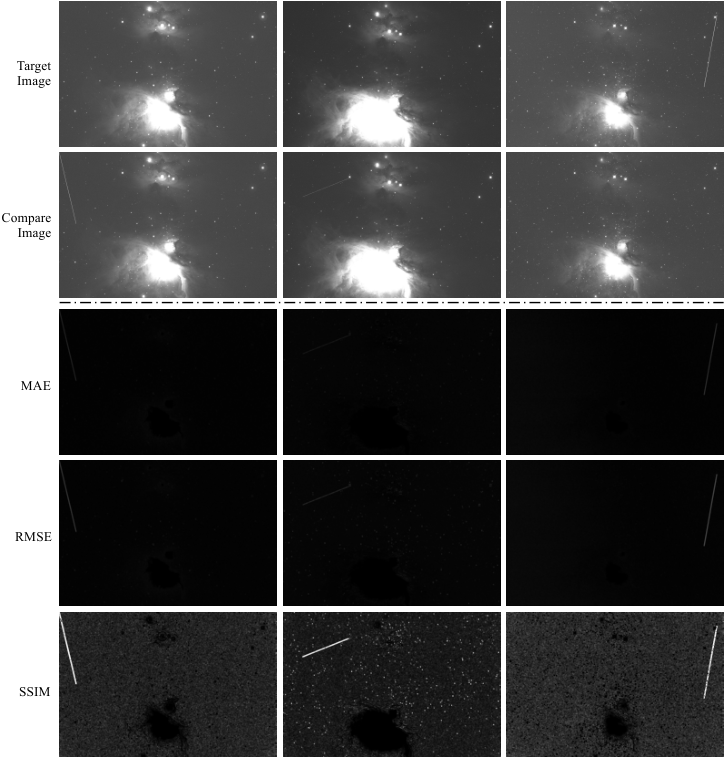
segmentation performance. Using only the inter-frame differential map already yields strong segmentation performance, and adding the heatmap further improves the results. Their combination performs best because the differential map suppresses persistent celestial structures while the heatmap guides trail localization. Additional sensitivity analysis is provided in Appendix 0.F.
| Method | mIoU |
| RMSE | |
| MAE | |
| ZOGY | |
| OIS | |
| DIA | |
| SSIM |
| Category | Method | mIoU | Dice | Prec. | Recall |
| Image-only segmentation | SAM† [20] | 0.358 | 0.528 | 0.449 | 0.640 |
| Synthetic supervision | PSF | 0.539 | 0.700 | 0.748 | 0.658 |
| Inter-frame representation | Otsu | 0.045 | 0.004 | 0.002 | 0.761 |
| Morph. | 0.158 | 0.270 | 0.172 | 0.630 | |
| Hough | 0.259 | 0.178 | 0.105 | 0.741 | |
| Localization cue | IRNet† [1] | 0.131 | 0.232 | 0.373 | 0.169 |
| SEAM† [38] | 0.039 | 0.074 | 0.106 | 0.057 | |
| Proposed | STARLINC | 0.485 | 0.653 | 0.815 | 0.545 |
6.2 Comparison of Inter-Frame Differential Maps
The inter-frame differential map is a central cue in STARLINC, suppressing persistent celestial content while highlighting frame-specific satellite trails. We compare the SSIM-based structural dissimilarity map with RMSE, MAE, and astronomy-oriented subtraction methods, including ZOGY [41], OIS [3], and DIA [8]. These methods are treated as differential-map alternatives rather than stand-alone segmentation baselines, since they produce difference images rather than binary masks. All variants use the same segmentation architecture and training setup, with only the differential-map construction changed.
As shown in Tab. 5, SSIM performs best among the differential maps. RMSE and MAE are sensitive to brightness fluctuations and residual stellar cores, while ZOGY, OIS, and DIA are mainly optimized for point-source variability and normalized subtraction. Since satellite trails are line-like outliers, SSIM better captures frame-specific structural changes than pixel-wise flux differences. Thus, the SSIM-based map provides a stronger masking cue, while physical subtraction methods may still require tuning for extended artifacts. Qualitative comparisons are provided in Figure 12.
6.3 Analysis of Alternative Designs
The three-channel design of STARLINC naturally suggests several alternatives. Instead of combining the original image , inter-frame differential map , and heatmap , we consider whether each cue can be used alone or replaced by an existing technique. We organize these alternatives by their target cue in Tab. 5.
Image-only segmentation.
A natural baseline is to apply a general-purpose segmentation model directly to the astronomical image. We evaluate SAM [20] as an image-only segmentation alternative, without using inter-frame differential maps or classifier heatmaps. As shown in Tab. 5, SAM obtains 0.358 mIoU and 0.528 Dice, which is below STARLINC. This suggests that generic image segmentation alone is insufficient for low-SNR satellite trail masking, where trails are thin and lack the object-like appearance priors of natural images.
Synthetic supervision.
We further examine whether improved synthetic-trail realism can enhance segmentation performance. For this purpose, we replace the geometric trail renderer with a PSF-aware renderer while keeping the remaining STARLINC pipeline unchanged. As shown in Tab. 5, PSF-aware rendering improves mIoU and Dice from 0.485/0.653 to 0.539/0.700, suggesting that more realistic synthetic trails can improve mask overlap. However, its lower precision relative to the main STARLINC configuration (0.748 compared with 0.815) suggests that these gains in overlap metrics are accompanied by reduced precision. We therefore include it as an additional analysis.
Inter-frame representation.
We assess whether the inter-frame differential map can serve as a direct basis for mask generation. Specifically, we apply Otsu thresholding, morphological filtering, and Hough-based line extraction to the differential map. Although these methods achieve relatively high recall (Tab. 5), their precision remains very low because residual stellar cores, detector artifacts, and background fluctuations also produce strong responses. This shows that the differential map is effective as a localization cue but requires a learned segmentation model to distinguish satellite trails from other transient structures.
Localization cue.
Since the heatmap provides coarse localization of trail-like regions, we examine whether it can be used for weakly supervised segmentation. We evaluate IRNet [1] and SEAM [38], which derive masks from classifier localization cues. Both perform substantially worse than STARLINC. Their activation maps typically capture only the most discriminative trail fragments, not the full thin trail extent. Instead, STARLINC uses the heatmap only as an auxiliary cue while obtaining pixel-level supervision from synthetic trail masks.
7 Conclusion
Satellite trail contamination is becoming a persistent problem for modern astronomical surveys as low Earth orbit constellations expand. We presented STARLINC, which leverages temporal redundancy across repeated observations to isolate transient satellite artifacts. Using inter-frame differential maps, synthetic trail generation, and activation-map-based pseudo-localization, STARLINC enables pixel-level segmentation without manually annotated masks from real survey data. Experiments on the 7DT dataset show clear gains over classical and learning-based baselines, and cross-dataset evaluations further demonstrate that STARLINC maintains strong performance across survey datasets, indicating strong generalizability. By selectively masking contaminated regions instead of discarding entire frames, STARLINC offers a practical and scalable approach for handling satellite-induced artifacts in large-scale astronomical surveys.
Acknowledgements
This work has been mainly supported by the Basic Research Laboratory Program through the National Research Foundation of Korea (NRF) funded by the Korea government (MSIT) (RS-2024-00416859). Jinho Lee is the corresponding author, and he is also funded by: RS-2024-00395134, RS-2024-00347394, RS-2026-25548502, RS-2026-25495605, RS-2025-00564840, RS-2023-00256081, RS-2026-25549926
References
- [1] (2019) Weakly supervised learning of instance segmentation with inter-pixel relations. In Proceedings of the IEEE/CVF conference on computer vision and pattern recognition, pp. 2209–2218. Cited by: §6.3, Table 5.
- [2] (2011) EDLines: a real-time line segment detector with a false detection control. Pattern Recognition Letters 32 (13), pp. 1633–1642. Cited by: §3.1.
- [3] (1998) A method for optimal image subtraction. The Astrophysical Journal 503 (1), pp. 325–331. Cited by: §6.2.
- [4] (2006) Satellite tracks removal in astronomical images. In Iberoamerican Congress on Pattern Recognition, pp. 892–901. Cited by: §3.3.
- [5] (2022) Analytical simulations of the effect of satellite constellations on optical and near-infrared observations. Astronomy & Astrophysics 657, pp. A75. Cited by: §1.
- [6] (2026) SPHEREx confirms predictions for artificial satellite trail pollution in low earth orbit. arXiv preprint arXiv:2605.27501. Cited by: §1.
- [7] (2025) Satellite megaconstellations will threaten space-based astronomy. Nature (), pp. . Note: Published online December 2025 External Links: Document Cited by: §1.
- [8] (2008) A new algorithm for difference image analysis. Monthly Notices of the Royal Astronomical Society: Letters 386 (1), pp. L77–L81. Cited by: §6.2.
- [9] (1986) A computational approach to edge detection. IEEE Transactions on Pattern Analysis and Machine Intelligence 8 (6), pp. 679–698. Cited by: §1, §3.1.
- [10] (2025) Artificial satellite trails detection using u-net deep neural network and line segment detector algorithm. Publications of the Astronomical Society of the Pacific 137 (9), pp. 094504. Cited by: §1, §3.3, Table 1.
- [11] (1972) Use of the hough transformation to detect lines and curves in pictures. Communications of the ACM 15 (1), pp. 11–15. Cited by: Table 6, §1, §3.1, Figure 6, Figure 6, Table 1.
- [12] (2019) DeepStreaks: identifying fast-moving objects in the zwicky transient facility data with deep learning. Monthly Notices of the Royal Astronomical Society 486 (3), pp. 4158–4165. Cited by: §3.3.
- [13] (2019) The zwicky transient facility: science objectives. Publications of the Astronomical Society of the Pacific 131 (1001), pp. 078001. Cited by: Appendix 0.B, 3rd item, §1, §5.4.
- [14] (2020) Impact of satellite constellations on astronomical observations with eso telescopes in the visible and infrared domains. Astronomy & Astrophysics 636, pp. A121. Cited by: §1.
- [15] (2018) Learning to parse wireframes in images of man-made environments. In Proceedings of the IEEE Conference on Computer Vision and Pattern Recognition, pp. 626–635. Cited by: Figure 13, Figure 13, Appendix 0.H, §2.2.
- [16] (2025) Dt-lsd: deformable transformer-based line segment detection. In 2025 IEEE/CVF Winter Conference on Applications of Computer Vision (WACV), pp. 3477–3486. Cited by: Table 6, §3.2, Figure 6, Figure 6, Table 1.
- [17] (2024) Detection of streaks in astronomical images using machine learning. Journal of Artificial Intelligence and Technology 4 (1), pp. 1–8. Cited by: §1, §3.3.
- [18] (2016) Astride: automated streak detection for astronomical images. Astrophysics Source Code Library, pp. ascl–1605. Cited by: §3.3.
- [19] (2024) Introduction to the 7-dimensional telescope: commissioning procedures and data characteristics. In Ground-based and Airborne Telescopes X, Vol. 13094, pp. 442–452. Cited by: Appendix 0.J, Appendix 0.B, 3rd item, §1, §5.1, §5.4.
- [20] (2023) Segment anything. In Proceedings of the IEEE/CVF international conference on computer vision, pp. 4015–4026. Cited by: §6.3, Table 5.
- [21] (2026) Starlink statistics. Note: Jonathan’s Space Pages https://planet4589.org/space/con/star/stats.htmlAccessed: 2026-02-18 Cited by: §1.
- [22] (2020) The low earth orbit satellite population and impacts of the spacex starlink constellation. The Astrophysical Journal Letters 892 (2), pp. L36. Cited by: §1.
- [23] (2021) Deep learning-based method to recognize line objects and flow arrows from image-format piping and instrumentation diagrams for digitization. Applied sciences 11 (21), pp. 10054. Cited by: §1.
- [24] (2022) Impact of the spacex starlink satellites on the zwicky transient facility survey observations. The Astrophysical Journal Letters 924 (2), pp. L30. Cited by: §1.
- [25] (2018) Optimal and efficient streak detection in astronomical images. The Astronomical Journal 156 (5), pp. 229. Cited by: §3.3.
- [26] (2026) Deep learning approach for automated detection of space objects in astronomical imaging. Astronomy and Computing 55, pp. 101081. Cited by: §1, §3.3.
- [27] (2020) MAXIMASK and maxitrack: two new tools for identifying contaminants in astronomical images using convolutional neural networks. Astronomy & Astrophysics 634, pp. A48. Cited by: Table 6, §3.3, Figure 6, Figure 6, Table 1.
- [28] (2023) Deeplsd: line segment detection and refinement with deep image gradients. In Proceedings of the IEEE/CVF Conference on Computer Vision and Pattern Recognition, pp. 17327–17336. Cited by: Figure 13, Figure 13, Table 6, Appendix 0.H, §1, §2.2, §3.2, Table 1.
- [29] (1986) On the determination of functions from their integral values along certain manifolds. IEEE transactions on medical imaging 5 (4), pp. 170–176. Cited by: Table 6, §1, §3.1, Table 1.
- [30] (2015) U-net: convolutional networks for biomedical image segmentation. In International Conference on Medical image computing and computer-assisted intervention, pp. 234–241. Cited by: §4.
- [31] (2008) LabelMe: a database and web-based tool for image annotation. International Journal of Computer Vision. Cited by: §5.2.
- [32] (2017) Grad-cam: visual explanations from deep networks via gradient-based localization. In Proceedings of the IEEE international conference on computer vision, pp. 618–626. Cited by: §4.3, §4.3.
- [33] (2024) Automated detection of satellite trails in ground-based observations using u-net and hough transform. Astronomy & Astrophysics 692, pp. A199. Cited by: Table 6, §1, §3.3, Table 1.
- [34] (2022) ELSED: enhanced line segment drawing. Pattern Recognition 127, pp. 108619. Cited by: §3.1.
- [35] (2021) Line detection via a lightweight cnn with a hough layer. In Thirteenth International Conference on Machine Vision, Vol. 11605, pp. 376–385. Cited by: §3.2.
- [36] (2012) Edge drawing: a combined real-time edge and segment detector. Journal of Visual Communication and Image Representation 23 (6), pp. 862–872. Cited by: §3.1.
- [37] (2010) LSD: a fast line segment detector with a false detection control. IEEE Transactions on Pattern Analysis & Machine Intelligence 32 (04), pp. 722–732. Cited by: Table 6, §3.1, Table 1.
- [38] (2020) Self-supervised equivariant attention mechanism for weakly supervised semantic segmentation. In Proceedings of the IEEE/CVF conference on computer vision and pattern recognition, pp. 12275–12284. Cited by: §6.3, Table 5.
- [39] (2000) The simbad astronomical database-the cds reference database for astronomical objects. Astronomy and Astrophysics Supplement Series 143 (1), pp. 9–22. Cited by: §2.1.
- [40] (2019) Learning attraction field representation for robust line segment detection. In Proceedings of the IEEE/CVF Conference on Computer Vision and Pattern Recognition, pp. 1595–1603. Cited by: §3.2.
- [41] (2016) Proper image subtraction—optimal transient detection, photometry, and hypothesis testing. The Astrophysical Journal 830 (1), pp. 27. Cited by: §6.2.
- [42] (2021) AG3line: active grouping and geometry-gradient combined validation for fast line segment extraction. Pattern Recognition 113, pp. 107834. Cited by: §3.1.
- [43] (2019) Ppgnet: learning point-pair graph for line segment detection. In Proceedings of the IEEE/CVF Conference on Computer Vision and Pattern Recognition, pp. 7105–7114. Cited by: §3.2.
- [44] (2021) Deep hough transform for semantic line detection. IEEE Transactions on Pattern Analysis and Machine Intelligence 44 (9), pp. 4793–4806. Cited by: §1, §3.2.
Appendix
Appendix 0.A Detailed Experiment Settings
We adopt a U-Net architecture with four encoder and decoder stages and three-channel inputs. The model is trained using the Adam optimizer with a batch size of 8 and an initial learning rate of for 200 epochs. Input images are padded to multiples of 32 to match the U-Net downsampling structure, and a threshold of 0.3 is applied during inference to obtain binary masks. All experiments are implemented in Python 3.11 using PyTorch 2.1 with CUDA 12.8 and are conducted on NVIDIA A6000 and RTX 4090 GPUs. During inference, STARLINC runs at 0.543s/img with 2.25GiB peak GPU memory.
Appendix 0.B Additional Cross-Dataset Generalization on Astronomical Observations
In this section, we evaluate the cross-dataset generalizability of STARLINC. The model used in this experiment is trained on our dataset and directly applied to astronomical images from different observational fields without additional retraining. Figure 9 shows qualitative examples from two different astronomical fields, Serpens and Messier 81. The Serpens images are drawn from the 7DT dataset [19], while the Messier 81 images are obtained from the IRSA archive [13].
Despite the differences in background structure and object distribution, STARLINC successfully localizes satellite trails while preserving surrounding celestial sources. In the Serpens example, STARLINC detects a very faint trail that is barely visible in the original image. In the Messier 81 example, the method reliably identifies multiple trails within a single frame, further demonstrating strong cross-dataset generalization to unseen fields and trail configurations. These results suggest that STARLINC is not restricted to a specific dataset or observational domain and can be effectively applied to diverse astronomical images.
Appendix 0.C Qualitative Results of Inter-Frame Differential Maps and Heatmaps

In this section, we present qualitative examples of the three input modalities used by the segmentation model: the original image, the mean inter-frame differential map, and the heatmap. Figure 7 illustrates these three representations across consecutive frames. The original image provides the full astronomical scene, including both static celestial objects and possible trail contamination. The mean inter-frame differential map (§ 4.2) is obtained by averaging pairwise SSIM distances between the target frame and other frames in the same observation group. This process emphasizes transient structures while suppressing static celestial objects that remain consistent across the group. The heatmap provides an additional localization cue derived from the classification model.
Frames containing satellite trails (, , ) exhibit a clear pattern. In these cases, the trail produces a strong response in the differential map because it appears only in the target frame and is absent from the comparison frame, creating a localized structural inconsistency. The heatmap also highlights regions around the trail, indicating that the classifier attends to trail-contaminated areas. In contrast, a trail-free frame such as exhibits only weak responses in both the differential map and the heatmap, indicating that both representations respond selectively to the presence of trails rather than to static background content.
These observations support our design choice for the segmentation input. The differential map captures temporal anomalies caused by moving satellite trails, while the heatmap provides complementary visual localization cues. Together, the differential map, heatmap, and original image form a complementary three-channel input for accurate trail segmentation.
Appendix 0.D Further Qualitative Comparison
In this section, we present additional qualitative comparisons as shown in Figure 11. While Figure 6 provides representative cases of satellite trail removal, Figure 11 presents a larger set of examples, enabling evaluation across a wider variety of trail appearances and background conditions.
Classical line detection methods such as Hough, Radon, and LSD frequently fail to robustly capture satellite trails in astronomical images. These approaches often produce false detections on bright celestial structures and galaxy edges, while missing faint or partially visible trails. Learning-based line detectors, including DeepLSD and DT-LSD, demonstrate improved sensitivity in some cases but still produce fragmented detections or unstable responses, especially when trails are weak or blended with dense background structures. Masking-based approaches such as ASTA and MaxiMask sometimes remove portions of the trail, but they often leave residual artifacts or remove excessive background regions, leading to excessive removal of valid astronomical data.
In contrast, STARLINC consistently produces cleaner and more coherent trail localization and removal results. The proposed method effectively captures the full extent of satellite trails while preserving surrounding celestial structures, even in challenging scenarios involving faint trails, complex backgrounds, and trails of varying brightness. These results highlight the robustness of STARLINC for practical satellite trail removal in real astronomical survey.
Appendix 0.E Classification-based Trail Detector Details
To provide localization cues for segmentation, we train a classification model as described in § 4.3 to generate heatmap-based representations. In this section, we report additional details and experimental results of the classifier.
0.E.1 Architecture and Training Details
For classification, we employ a ResNet-34 backbone trained using the Adam optimizer with an initial learning rate of and a batch size of 8 for 50 epochs. A ReduceLROnPlateau scheduler is applied with a reduction factor of 0.5 and patience of 5 epochs, with a minimum learning rate of .
As described in § 4.1, synthetic satellite trails are injected into clean images to balance the training distribution. This augmentation mitigates the inherent class imbalance in satellite trail detection and facilitates stable training of the classification model.
| Category | Method | Metrics | |||||
| Acc | Pre | Recall | F1 | ROC-AUC | PR-AUC | ||
| Classical | Hough [11] | 0.875 | 0.913 | 0.429 | 0.583 | 0.692 | 0.756 |
| Radon [29] | 0.863 | 0.944 | 0.347 | 0.507 | 0.671 | 0.708 | |
| LSD [37] | 0.204 | 0.204 | 1.000 | 0.339 | 0.777 | 0.723 | |
| Learning-based | DeepLSD [28] | 0.204 | 0.204 | 1.000 | 0.339 | 0.868 | 0.834 |
| DT-LSD [16] | 0.917 | 1.000 | 0.592 | 0.744 | 0.796 | 0.838 | |
| Trail detection | ASTA [33] | 0.429 | 0.244 | 0.857 | 0.380 | 0.677 | 0.384 |
| MaxiMask [27] | 0.913 | 0.967 | 0.592 | 0.734 | 0.795 | 0.830 | |
| Proposed | STARLINC (Ours) | 0.983 | 0.959 | 0.959 | 0.959 | 0.998 | 0.996 |
0.E.2 Evaluation on Satellite Trail Classification
Beyond segmentation, we evaluate the classifier stage of STARLINC, which serves as an upstream detector and provides image-level predictions and localization cues through a heatmap to the segmentation module. Table 6 summarizes the results, and Appendix (Figure 8) provides the ROC and PR curves.
Overall, classical detectors exhibit a clear precision–recall trade-off. Hough and Radon achieve high precision (0.913/0.944) but low recall (0.429/0.347), while LSD over-triggers positives (precision 0.204). Learning-based baselines improve performance, with DT-LSD achieving the strongest results among them (F1 0.744), whereas DeepLSD shows over-detection consistent with the domain gap. Trail-specific methods are mixed: ASTA degrades on 7DT (F1 0.380) and MaxiMask is more competitive (F1 0.734) but remains limited in recall.
STARLINC achieves the best performance across all metrics (accuracy 0.983, F1 0.959, ROC-AUC 0.998) with balanced precision and recall (0.959/0.959). We further provide ablation study of classification pipeline in Tab. 8. The results show that removing synthetic trail generation and the inter-frame differential map degrades performance, while combining them yields the best results, indicating complementary benefits.
0.E.3 Additional Experimental Results of the Classifier
| Synthetic ratio (%) | Number of data | |||||
| 150 | 300 | 450 | 600 | 750 | 900 | |
| 30 | 0.651 | 0.863 | 0.835 | 0.863 | 0.882 | 0.865 |
| 50 | 0.515 | 0.653 | 0.662 | 0.756 | 0.824 | 0.959 |
| 70 | 0.626 | 0.626 | 0.492 | 0.364 | 0.492 | 0.545 |
| 90 | 0.371 | 0.339 | 0.345 | 0.344 | 0.344 | 0.375 |
| Method | Metrics | ||||
| § 4.1 | § 4.2 | F1 | Acc | Pre | Recall |
| ✗ | ✗ | 0.314 | 0.708 | 0.302 | 0.327 |
| ✓ | ✗ | 0.381 | 0.783 | 0.457 | 0.327 |
| ✗ | ✓ | 0.779 | 0.913 | 0.804 | 0.755 |
| ✓ | ✓ | 0.959 | 0.983 | 0.959 | 0.959 |
Figure 8 further illustrates the classification performance using ROC and PR curves, complementing the quantitative results presented in subsection 0.E.2. The curves show that the proposed classifier maintains a favorable precision–recall trade-off across different decision thresholds.
Tab. 7 presents the sensitivity analysis of the classification detector with respect to the synthetic data ratio and the number of training samples. All results are reported in terms of the F1 score. Overall, increasing the number of training samples generally improves performance, particularly when the dataset size increases from 150 to 450 samples, indicating that the classifier benefits from additional training data.
Among the tested configurations, a synthetic ratio of 50% achieves the best overall performance, reaching the highest F1 score of 0.959 when 900 training samples are used. This suggests that a balanced mixture of real and synthetic samples provides the most effective training signal for the detector.
In contrast, higher synthetic ratios (e.g., 70% and 90%) lead to noticeably degraded performance across most dataset sizes. This indicates that excessive reliance on synthetic samples may introduce a distribution mismatch with real astronomical images, ultimately harming detection performance. Based on these observations, we adopt a synthetic ratio of 50% and 900 training samples as the default configuration for the classification detector.
Appendix 0.F Synthetic Fraction Sensitivity
Tab. 9 reports the sensitivity analysis of the segmentation model with respect to the fraction of synthetic trail images among total trail images. This quantity mainly controls the class balance between trail and non-trail images. To directly evaluate the effect of synthetic trails, we vary the synthetic fraction among trail-containing images and report the segmentation performance in Table 9. The reference STARLINC setting corresponds to a synthetic fraction of 57.3%.
| Synthetic fraction (%) | 57.3 | 65.1 | 70.0 | 75.1 | 80.0 | 85.1 | 90.0 | 95.1 |
| mIoU |
The results show that STARLINC is not highly sensitive to the fraction of synthetic trails among trail-containing images. Even at 95.1% synthetic trails, the model achieves 0.504 mIoU, which is comparable to the reference setting. These results support the use of synthetic trail injection as a scalable source of pixel-level supervision. At the same time, the synthetic trail realism study in § 6.3 shows that improving the rendering model, such as by adding PSF-aware trail profiles, can further improve real-image segmentation performance.
Appendix 0.G Fine-tuned Baseline Results
For completeness, we report the 7DT results of the fine-tuned learning-based baselines.The baselines include DeepLSD, DT-LSD, ASTA, and MaxiMask, which are adapted to the target 7DT setting. As shown in Tab. 10, fine-tuning improves the applicability of existing line or trail detectors to astronomical images, but their performance remains below STARLINC. These results indicate that adapting existing detectors alone is insufficient for robust pixel-level satellite-trail segmentation on 7DT observations.
| Method | mIoU | Dice | Precision | Recall |
| DeepLSD† | 0.269 | 0.380 | 0.293 | 0.628 |
| DT-LSD† | 0.381 | 0.474 | 0.482 | 0.477 |
| ASTA† | 0.285 | 0.394 | 0.360 | 0.506 |
| MaxiMask† | 0.220 | 0.289 | 0.734 | 0.180 |
Appendix 0.H Additional Motivational Results on Low-SNR Images
In this section, we present qualitative examples of how decreasing SNR degrades line detection. To generate images with controlled SNR levels, we inject synthetic noise into the original images. Specifically, background noise is modeled using a Gaussian component, and the noise magnitude is adjusted to achieve a desired target SNR level. For each image, a target SNR () is specified, and the noise standard deviation () is tuned such that the effective SNR of the resulting image approximates . This procedure allows us to systematically construct low-SNR samples that mimic challenging observational conditions frequently encountered in astronomical imaging, such as weak linear structures and increased background fluctuations.
Figure 13 shows predictions of DeepLSD [28] on the Wireframe dataset [15] under different SNR levels, alongside ground truth annotations. As the SNR decreases, structural line patterns become increasingly difficult to distinguish from background noise, causing the detector to miss valid segments and produce fragmented or unstable predictions. These results highlight the inherent difficulty of reliably detecting lines in low-SNR environments.
While modern line detectors perform well on natural images with relatively clean edges, their accuracy degrades substantially when the signal is weak relative to the background noise, a condition frequently encountered in astronomical observations. This motivates the development of methods robust to low-SNR conditions for satellite trail detection.
Appendix 0.I Network Size Sensitivity
We evaluate the sensitivity of STARLINC to the size of the U-Net segmentation backbone by varying the number of parameters while keeping the rest of the pipeline fixed.
| # Params(M) | 3.67 | 4.67 | 5.94 | 6.82 | 7.76 (Ours) | 8.96 | 10.97 | 20.61 |
| mIoU | 0.475 | 0.480 | 0.480 | 0.488 | 0.485 | 0.480 | 0.483 | 0.473 |
As shown in Table 11, the mIoU remains stable across the tested U-Net sizes, varying only from 0.473 to 0.488, with only minor drops at the smallest and largest scales. This stability suggests that the performance is driven more by the three-channel input representation than by increasing the segmentation backbone size, and we therefore use the 7.76M-parameter U-Net as the default setting.
Appendix 0.J Effect of Input Bit Depth
We further examine whether the 8-bit preprocessing used in the main pipeline limits the detection of faint satellite trails. This concern is important because astronomical CCD images are commonly stored with higher bit depth, whereas display-oriented 8-bit conversions may compress or clip low-contrast flux variations. Such loss could be especially harmful for trails close to the noise floor.
We focus on detectable faint trails with SNR , following the common observational convention that signals below this level are close to the sensitivity limit of ground-based telescopes and are difficult to distinguish reliably from background noise [19]. This threshold defines the regime where a visual or algorithmic trail label is meaningful, rather than a limitation specific to STARLINC.
To test whether bit-depth conversion is the dominant performance bottleneck in our setting, we evaluate a 16-bit variant of STARLINC using the same overall training and inference pipeline. As shown in Table 12, the 16-bit variant achieves comparable but slightly lower performance than the main 8-bit setting. This suggests that bit depth alone does not explain the remaining missed trail pixels in our current pipeline. One possible reason is that long, coherent linear structures remain detectable after 8-bit scaling when their SNR is above the target threshold, whereas other factors, such as residual stellar structures, seeing variation, and the training distribution, also affect segmentation quality.
We therefore use the 8-bit setting as the reference configuration for the main experiments, while treating FITS-native or fully 16-bit processing as an important direction for future work. In particular, future pipelines may benefit from jointly optimizing bit-depth handling, normalization, and faint-trail supervision rather than changing the input representation alone. The predicted masks from the main 8-bit pipeline can also be applied directly to the original FITS images, so the 8-bit representation is used for mask prediction rather than for replacing the scientific data product.
| Setting | mIoU | Dice | Precision | Recall |
| STARLINC-8bit(ours) | 0.485 | 0.653 | 0.815 | 0.545 |
| STARLINC-16bit | 0.450 | 0.621 | 0.816 | 0.501 |
Appendix 0.K Data Preservation through Pixel-Level Trail Removal
Conventional survey pipelines often discard entire exposures once satellite trails are detected. Although this prevents contamination from propagating into downstream analysis, it also leads to substantial data loss because valid astronomical information outside the trail region is removed together with the artifact.
| Baseline | Ours | |
| Ratio | 79.58% | 99.95% |
As discussed in Sec. 1, the number of LEO satellites is rapidly increasing, implying that the fraction of contaminated exposures will continue to grow. Under such conditions, image-level removal becomes increasingly inefficient, as a larger portion of the observational data would be discarded. In contrast, the proposed method removes satellite trails at the pixel level, allowing uncontaminated regions of the image to remain usable for scientific analysis. To quantify this effect, we measure the preservation ratio defined as the fraction of pixels that remain usable after artifact removal. Appendix 0.K compares this metric between conventional image removal and the proposed approach. While the conventional strategy retains only about 79.58% of the data due to full-image rejection, our method preserves approximately 99.95% of valid pixels by selectively masking the trail region. This difference highlights the practical advantage of pixel-level artifact removal, which becomes increasingly important for future large-scale surveys where the frequency of satellite contamination is expected to rise.
Appendix 0.L Limitations
In this work, we evaluate STARLINC using the available astronomical datasets containing satellite trails. However, the evaluation scope is currently limited by the availability of public datasets. Many modern astronomical observations remain proprietary to the survey teams that collected them and are typically released only after a proprietary period. As a result, comprehensive evaluation across a wider range of observational datasets is still limited at present. As more astronomical survey become publicly available in the future, broader validation across diverse astronomical observations would further demonstrate the applicability of STARLINC.