Machine Learning Unveils Finite-volume Energy Shifts in Three-body System
Abstract
Finite-volume extrapolation (FVE) is essential for extracting physical observables in the lattice calculation. While rigorous FVE formulations are well established for short-range potentials in both two- and three-body systems, long-range interactions with force ranges comparable to the lattice size remain challenging. Extending a previous data-driven scheme for two-body systems, we apply symbolic regression (PySR) to uncover universal three-body FVE formulae. For short-range potentials, we reproduce the two limiting cases, i.e. and . For pure long-range potentials, we obtain a dedicated analytic expression, and after incorporating short-range contributions, we uncover a unified formula consistent with the original PySR solution, which performs excellently in the intermediate force range around 1 fm. This work demonstrates that combining machine learning with physical constraints can yield novel analytical results inaccessible to conventional theoretical tools, advancing data-driven methodologies in hadron physics.
I Introduction
Lattice effective field theory (LEFT) provides an alternative framework in which nucleons, rather than quarks and gluons, are placed on a discretized spacetime lattice. The interactions between nucleons are organized according to chiral effective theory, and ground-state properties are computed via Auxiliary-Field Quantum Monte Carlo simulations [1]. A central challenge in LEFT, as in any other lattice calculations, is finite-volume effects. For few-body systems, the Lüscher formalism and its extensions to composite particles [2] provide analytic control over volume dependence, with topological corrections that depend only on the mass ratios of the constituents. For medium-mass nuclei, systematic Euclidean time extrapolation (“triangulation”) using multiple trial states enables reliable extraction of infinite-volume observables [3, 4]. More recently, symmetry sign extrapolation has extended these methods to neutron-rich systems [5]. Volume extrapolation in LEFT corrects for the finite-volume contamination, ensuring that the observables converge to their infinite-volume limits.
As the result, finite-volume extrapolation (FVE) is the bridge combining the results from finite volume and infinite volume and it can also extract some physical observables. In two-body system, FVE for short-range potential case has been derived by Lüscher formula [6]. However, the long-range interactions, in which force range is comparable to the box size and light particles serve as mediators in scattering states, present non-negligible challenges caused by the changeable force range and the significant partial wave mixing [7]. A typical example is the light-meson exchange in system [8]. Two methods struggle to explore the law of FVE, one is modifying Lüscher formula numerically by rewriting the zeta function and separating short-range and long-range potential [9, 10, 11, 7, 12, 13], the other is handling long-range interactions within the Hamiltonian framework and constructing irreducible representations and solve Lippmann-Schwinger equation to extract phase shifts [14]. However, neither approach yields a general formula. In three-body system, studies for short-range potential bound states have been thoroughly studied [15, 16, 17, 6, 18, 19] and present the formula in unitary limit by solving Schrödinger equation [15], or adopt effective field theory based on particle-dimer picture to derive FVE in two extreme situations [19, 16]. For example, there exists a bound state using effective field theory approach, a short-range repulsive three-body force is included [20]. Nevertheless, unlike two-body system, FVE in three-body system for long-range potential faces is a more complicated situation due to the disruption of the invariance of the Efimov continuous scale in finite volume [21].
Symbolic regression (SR) [22] can be applied to solve these problems; its advantages include the ability to uncover mathematical relationships from data [23] which has already exhibited its strengths in physics field [24]. Based on the genetic programming [25] a vast space containing variables, constants and signs can be searched and finally a new formula is constructed [26]. Compared with the traditional SR, some mathematics operations,i.e., symmetry, additive or multiplicative separability, variable substitution and modularity are utilized to add the physics limit and forge to present more effective results. For example, PhyE2E algorithm successfully improves the solar activity formula and discovers new analytical expressions for star formation rates from the simulation of the FIRE-2 galaxy [27]. AI Feynman algorithm combing with neural networks, large language model, deep learning and some necessary physics limits, perfectly derived more than 100 equations in Feynman Lectures on Physics [28, 29]. In fact, its capability of generating mathematical expression has been widely used and accelerated the researches in high-energy physics [30, 31]. For instance, model building and background fitting for data processing in experiments [32, 33, 34]. SR prompts rediscovery of dual relation of Kawai–Lewellen–Tye and Bern–Carrasco–Johansson in scattering amplitudes [35]. Fragmentation functions extracted from data are good candidates for global fitting [36]. Besides, SR plays a vital role in exploring Beyond the Standard Model (BSM) physics [37, 38], unveiling deeper relationships like constants of standard model [39] and Feynman integral singularities [40], exploring unknown phenomena like Tsallis distribution [41].
FVE formula for short-range potential in two-body system has already reproduced by neural network [42]. We have already rediscovered the FVE formula derived by Lüscher formula and have found a general formula in both short-range and long-range potentials by SR in two-body system [43]. The similar method is utilized in three-body system in our research. Before applying SR, samples need to prepared. Hadron Lattice Effective Field Theory (HLEFT) [20], which is analogous to Nuclear Lattice Effective Field Theory (NLEFT) [44, 45, 46], a powerful method for ab initio nuclear structure calculation [46] combining Chiral Effective Field Theory and Lattice quantum Monte Carlo (QMC) [1, 47, 48] to solve many-body problems. Continuous spacetime is discretized on a lattice where nucleons are placed [45] and the interaction between nucleus originates from Chiral Perturbation Theory.
NLEFT has already demonstrated its irreplaceable role in exploring structures and interactions in nucleus, especially in some characteristics of nucleon like its ground states [49, 50, 51, 3, 52, 53, 54] and excited states [55, 56, 57, 58], distributions of nuclear intrinsic density and clustering phenomena [59, 60, 61, 62, 63], scattering of nucleus-nucleus [64, 65], investigation of both zero-temperature and finite-temperature nuclear matter properties [66, 67, 68, 69] calculation of -cluster structure and light nuclei [1, 48, 70, 71, 47] explanation of exotic quantum phase transition [1, 72] and structure of exotic nucleon [73, 74]. The researches have also been expanded to hypernuclear systems [20, 75, 76, 74]. However, FVE challenges still exist in nucleon system.
In Ref. [43], we have already discussed FVE formula using SR in two-body identical bosons system, and SR provides the result combining short-range and long-range potential. Following the approach in two-body system, in this work, we introduce SR approach to study FVE formula in three-body identical bosons system, our workflow can be divided into these parts below. In Sec. II, we introduce the samples, generated in limited box sizes, for both short-range and long-range potential cases. The details of SR are presented in Sec. III. In Sec. IV, we describe the discovery of three-body FVE formulae applicable to both short-range and long-range potentials, deriving a unified formula.
II Samples Generation
For a simplicity, we consider a system of three identical spinless particles under a non-relativisitc framework. All the particles masses are set to . Considering only the pairwise interactions, the short-range potential in coordinate space takes the form:
| (1) |
where is the relative coordinate between the th and th particles in the center-of-mass frame. represents the strength of potential. From the effective field theory point of view, for the potential , a physical cutoff is needed to distinguish the short-range contribution from the long-range one, which keeps the renormalization group invariant. Here a single-particle regulator [77, 78, 79] can be utilized, where exp [80] is a soft cutoff function with and the momenta of the incoming and outgoing of the th particle [20]. Thus the Hamiltonian can be written as:
| (2) |
where is the mass of the th particle, is the transferred momentum of the two particles and () represents the relative incoming (outgoing) momentum between () and (). The corresponding potential in momentum space = can be obtained by a Fourier transformation from the expression in coordinate space.
In our framework, HLEFT [20] is used to generate the samples for both short-range and long-range potentials. The solution of the Schrödinger equation can be obtained by directly diagonalizing the Hamiltonian defined on lattice coordinate space. The matrix exact diagonalization scheme borrows the implicitly restarted Lanczos method, which finds the eigenvalues and eigenvectors [81] by SciPy [82] in Python. In short-range potential case, we perform simulations on cubic lattice . The potential strength has various values to generate the samples. More details of these samples are listed in Appendix A.

In the case of long-range potential, in each pair of particles, we define the potential like Yukawa potential form [9],
| (3) |
where reflects the range of the force. and are the strengths of the short-range potential and long-range potential. For simplicity, we set when generating samples. The details of the ranges of the force and values can be found in Appendix A. The reason of the existence of a short-range potential term in Eq. (3) is due to the divergence of the Yukawa potential in , which means that it needs a regularization. Similarly to the short-range potential case, a reasonable cutoff is applied, which gives reasonable physical observables. For the short-range potential term, is still applied to each pair of particles. At the same time, the regulator of the long-range potential 11 1 Here, is the cutoff to regularize the long-range potential, which is set equal to that for the short-range one above. is = exp [8, 83]. With the definition of the regulators, the Hamiltonian can be written as:
| (4) |
Here, both the short-range potential and the long-range potential can be transformed into their coordinate forms by Fourier transformation. The simulations are performed in cubic lattice of box sizes fm3. Finally, analogous to our treatment for the pure short-range potential case, we solve the Schrödinger equation and extract the finite-volume binding energy via the HLEFT. Representative examples are provided in Appendix A.
III Symbolic Regression
Samples generated by HLEFT are performed for SR to explore FVE formula. SR model based on genetic algorithms (GA) [84, 85] and can search for the mathematical relationship between inputs and outputs through multi-population evolutionary [26]. PySR model [86] explores the analytic expression space constructing by the sets of input(output) variables, constant terms and operators. The input variable here is box size and the output variable is binding energy . The operators contain addition, multiplication, division, exponential, sqrt, cube and some custom-defined operators. Compared with the massive samples utilized in deep learning, few samples are sufficient for PySR. The model performs 200 iterations of 200 different population samples, with each population containing 100 individuals. The evaluation of the output formula contains two vital elements: loss and complexity. Loss is used to measure how well the output formula describes the samples, which is defined as mean square error (MSE):
| (5) |
Here, is the formula output by the PySR model, and is the energy of a system in a box of size calculated by HLEFT. Complexity is an indicator for measuring the degree of redundancy in a formula. Values of complexity for each variable, constant and operator can be set. PySR model combines these two elements and evaluates the formula using score, which rewards minimal loss and penalizes more complicated formula. It can be defined as
| (6) |
Here, is the complexity 22 2 The upper limit of the value can be set larger to allow higher order contributions as that in analytic analysis [6]. (each complexity of variables, constants and operators can be found in the Appendix B), which is defined as the total number of operations, variables, and constants used in a formula. Score can help PySR choose the best formula.
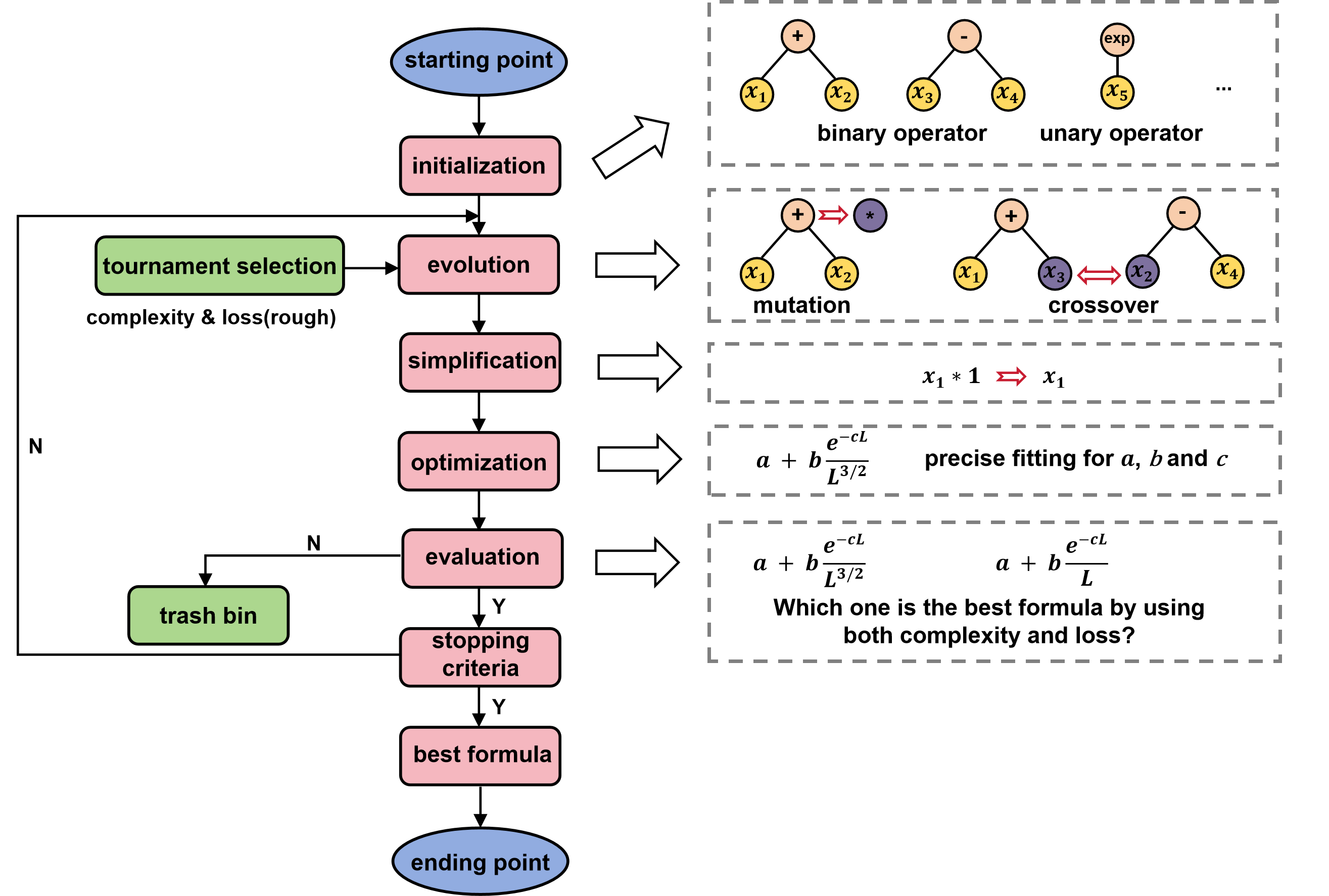
The whole evolution process in PySR is similar to the process in nature. 200 populations are included in evolutions and each of them has their own mechanism. For each evolution, initial formulae are randomly constructed by variables, constants and operators and experience mutations and crossovers in each iteration. PySR chooses some performed-well individuals as the parents for next iteration until triggering the stop condition set before. Each evolution process can be seen in Fig. 1. Different evolutions happen at the same time and populations exchange some elements and the best formula can be chosen through this process.
IV Results
As discussed in the previous section, we consider three identical spinless bosons with mass , forming a bound state with binding momentum , interacting via two-body forces only. The generated samples for short-range potential case input to PySR model, the best result presented by PySR is:
| (7) |
Here are free parameters, with representing the binding energy in the infinite-volume limit, and characterizing to the wave-function normalization coefficient, and scaling with the binding momentum. In fact, in short-range potential case, theoretical research of FVE formula has already reached conclusions [15, 19]. FVE formula depends on both two-body binding momentum and three-body binding momentum . Under unitary limit (), theoretical formula is obtained based on Lüshcer method in Ref. [6]. By solving the three-body Schrödinger equation in a finite cubic box and employing the asymptotic form of the infinite-volume three-body bound state wave function, the exponential decay behavior of the energy correction is obtained [15].
| (8) |
Here, represents the binding energy in infinite volume. is the free parameter. For the case each pair of particles is tightly bound, i.e. , formula [19] in short-range potential is governed by:
| (9) |
To compare the performance of different formulae against the samples, we present the fitting results in Fig. 2 for the short-range potential using three candidate expressions: Eq. (7) (pink dashed line), Eq. (8) (orange dashed solid line), and Eq. (9) (seagreen long-dashed line). The gray dot-dashed line is the fitting result of in Eq. (7), which represents . For all samples of different strength of potential , Eq. (7) provides the best description of these samples across the full ranges of box sizes compared with Eq. (8) and Eq. (9).
Taking it a step further, we analyze the properties of the parameters in Eq. (7), especially the power of in the third term, the important ratio between the third term compared and the second term. and values with different potential strengths are shown in Fig. 3. Here, the blue dots and the red squares represent the parameters and in Eq. (7), respectively. It can be seen that when the potential strengths increases from 2.0 to 2.9 , parameter gradually decreases and converges to 1, which approaches to that in Eq. (9) as . In contrast, when the potential strengths decrease from 2.9 to 2.0 , ratio gradually decreases and converges to 0, which recover the formula in Eq. (8), i.e. the case of . It should be noted that, is strongly correlated with the momentum ratio . In Fig. 3, the region where the color approaches colorless indicates that and approaches orange means . A smaller value of indicates the more loosely bound states for three-body system, whereas a larger value of represents more tightly binding for two-body subsystem. Thus, when three particles bind as a loosely bound state, i.e., , the second term of the Eq. (7) plays the main role, i.e., , and if two-body subsystem tightly binds together, i.e., , the third term of the formula plays the main role, i.e., , which has rediscovered the theoretical formula Eqs. (8) and (9). However, the LEFT data considered here do not reach either of the two extreme regimes, and ; consequently, the exponent is distinct from both the exponent in Eq. (8) and that in Eq. (9). Nevertheless, within uncertainties, still lies between these two values. Finally, our results show that between these two extreme situations, there’s a linear combination of Eqs. (8) and (9) in the intermediate region. All the results of data mentioned above are listed in Appendix C.
For long-range potential, we set force range parameter to three values, which correspond to the force ranges of about 3, 5, 8 fm, and then generate samples and feed them into PySR model. The best result presented by PySR is:
| (10) |
Here, are free parameters. The fitting results for long-range potential samples using this formula are listed in Fig. 4, described by the purple dashed line, which matches well with the samples in both small box sizes and large box sizes. The gray dashed line is the fitting value of in Eq. (10), which represents . Overall, the Eq. (10) provides a robust and physically meaningful description of the system.
However, the contribution of short-range potential in the FVE formula should not be ignored. Based on the theoretical formula [15, 19] from short-range potential case, i.e., Eqs. (8) and (9), our formula is rewritten as,
| (11) |
keeping the last two terms as the short-range expression. Here, are free parameters, and represents , the second term represents the contribution of the long-range, while the third and fourth terms represent the contribution of the short-range potential. The fitting results for the long-range potential samples are also listed in Fig. 4, with the pink dashed line representing Eq. (11) and the orange line showing the contribution of the short-range potential in Eq. (11). For all samples of different strength of potential , Eq. (11) provides well description of these samples, and similar to Eq. (10). It’s worth mentioning that the contribution of the short-range potential in Eq. (11) hardly affect the fitting results.
Taking a further step, we analyze the properties of the parameters in Eq. (10) and Eq. (11), especially the parameters , and , in the contribution of long-range potential in the second term. The fitting results of the parameters for all samples with different potential strengths and force ranges are shown in Fig. 5. Here, the dots(triangles) and diamonds(squares) represent the parameters () and () in Eq. (10) and Eq. (11), respectively. Fitting results of samples with force ranges of about 3, 5, and 8 fm, distinguished by red, blue, and green, respectively. It can be seen that the values of parameters and are close to each other, and so are those of and . This shows that the contribution of the short-range potential in Eq. (11) hardly affect the fitting results. It’s worth mentioning that, parameters and correlate with both the range of the force and the strength of the potential. Particularly, their absolute values are positively correlated to the force range and the force strength. In contrast, and depend almost entirely on the range of the force and are negatively corrected with it. The behavior of all the parameters indicates that the correction of FVE is positively correlated with the range of the force, which matches what we expect physically. It follows that, Eq. (10) is equivalent to Eq. (11) in long-range potential case, and PySR gives a simple FVE formula.
To explore the reliability of our formula, i.e. Eq. (11), when the samples with a force range tend to be short-range, we specifically generate samples by HLEFT with a force range of about 1 fm and fit them. The fitting results are presented in Fig. 6. Here, the pink long-dashed line, orange short-dashed line and seagreen dashed line correspond to Eq. (11), its short‑range contribution and its long‑range contribution, separately. The gray dashed line is the fitting value of in Eq. (11). It should be noted that, since the samples satisfies , the short-range contribution in our formula only considers the third term of Eq. (11) for fitting. For all samples of different strength of potential , Eq. (11) provides well description of these samples. Compared to the fitting results of the samples with force range of 3, 5, 8 fm in Fig. 4, the short-range contribution of Eq. (11) significantly increases in 1 fm case. Due to the short-range contributions, the values of parameters and for the long-range contribution do not follow the rules in Fig. 5. Overall, in order to find a unified formula to describe the finite volume effects of samples under different force ranges, the formula needs to include contributions of both short-range and long-range terms, as shown in Eq. (11).
V Summary and Outlook
FVE is a vital step to extract some physical observables for lattice calculations. In two-body system and three-body system, FVE has been rigorously derived in the case of short-range potential. However, challenge exists in long-range potential, especially when the range of the force is comparable to the box size . Several works on two-body system have numerically modified Lüscher formula to extract the FVE formula but a gap still remains in three-body system. Two-body system has already explored a general formula by SR and the same way are utilized in three-body system.
In short-range potential, formulae in theory are well rediscovered for two extreme cases, i.e., and , and between these two situations, the formula is the liner combination of these two cases, which is greatly influenced by the strength of short-range potential. For the long-range potential, PySR yields the expression given in Eq. (10). Once short-range potential contributions are included, the formula can be recast into Eq. (11), which is equivalent to the original PySR solution. In the intermediate force range (approximately 1 fm), Eq. (11) exhibits outstanding performance. Consequently, Eq. (11) can serve as a general formula for describing three-body systems.
Our work makes a notable step forward in the application of data-driven methodologies to explore previously inaccessible regimes in particle physics. By integrating modern learning architectures with physical priors, we demonstrate a viable pathway toward discovering novel signatures that lie beyond the reach of conventional analytical tools.
VI Acknowledgments
This work was supported in part by the National Natural Science Foundation of China (Grant Nos. 12375073, 12547105, and 12375072); CAS Project for Young Scientists in Basic Research (Grant No. YSBR-117).
References
- [1] T. A. Lähde and U.-G. Meißner, Nuclear Lattice Effective Field Theory: An introduction, Vol. 957 (Springer, 2019).
- [2] S. Bour, S. Koenig, D. Lee, H. W. Hammer, and U.-G. Meissner, Topological phases for bound states moving in a finite volume, Phys. Rev. D 84, 091503 (2011).
- [3] T. A. Lähde, E. Epelbaum, H. Krebs, D. Lee, U.-G. Meißner, and G. Rupak, Lattice effective field theory for medium-mass nuclei, Phys. Lett. B 732, 110 (2014a).
- [4] T. A. Lähde, E. Epelbaum, H. Krebs, D. Lee, U.-G. Meißner, and G. Rupak, Uncertainties of Euclidean time extrapolation in lattice effective field theory, J. Phys. G 42, 034012 (2015a).
- [5] T. A. Lähde, T. Luu, D. Lee, U.-G. Meißner, E. Epelbaum, H. Krebs, and G. Rupak, Nuclear lattice simulations using symmetry-sign extrapolation, Eur. Phys. J. A 51, 92 (2015b).
- [6] M. Lüscher, Volume dependence of the energy spectrum in massive quantum field theories. 1. stable particle states, Commun. Math. Phys. 104, 177 (1986).
- [7] R. Bubna, H.-W. Hammer, B.-L. Hoid, J.-Y. Pang, A. Rusetsky, and J.-J. Wu, Modified Lüscher zeta-function and the modified effective range expansion in the presence of a long-range force, JHEP 10, 197.
- [8] L. Meng, V. Baru, E. Epelbaum, A. A. Filin, and A. M. Gasparyan, Solving the left-hand cut problem in lattice QCD: from finite volume energy levels, Phys. Rev. D 109, L071506 (2024).
- [9] R. Bubna, H.-W. Hammer, F. Müller, J.-Y. Pang, A. Rusetsky, and J.-J. Wu, Lüscher equation with long-range forces, JHEP 05, 168, arXiv:2402.12985 [hep-lat] .
- [10] S. M. Dawid, F. Romero-López, and S. R. Sharpe, Finite- and infinite-volume study of scattering, JHEP 01, 060.
- [11] F. Romero-López, A. Rusetsky, N. Schlage, and C. Urbach, Relativistic -particle energy shift in finite volume, JHEP 02, 060.
- [12] T. Iritani, S. Aoki, T. Doi, T. Hatsuda, Y. Ikeda, T. Inoue, N. Ishii, H. Nemura, and K. Sasaki (HAL QCD), Consistency between Lüscher’s finite volume method and HAL QCD method for two-baryon systems in lattice QCD, JHEP 03, 007.
- [13] K. Yu, G.-J. Wang, J.-J. Wu, and Z. Yang, Finite volume Hamiltonian method for two-particle systems containing long-range potential on the lattice, JHEP 04, 108.
- [14] L. Meng and E. Epelbaum, Two-particle scattering from finite-volume quantization conditions using the plane wave basis, JHEP 10, 051.
- [15] U.-G. Meißner, G. Ríos, and A. Rusetsky, Spectrum of three-body bound states in a finite volume, Phys. Rev. Lett. 114, 091602 (2015), [Erratum: Phys.Rev.Lett. 117, 069902 (2016)].
- [16] H.-W. Hammer, J.-Y. Pang, and A. Rusetsky, Three-particle quantization condition in a finite volume: 1. the role of the three-particle force, JHEP 09, 109.
- [17] M. T. Hansen and S. R. Sharpe, Applying the relativistic quantization condition to a three-particle bound state in a periodic box, Phys. Rev. D 95, 034501 (2017).
- [18] S. König and D. Lee, Volume dependence of -body bound states, Phys. Lett. B 779, 9 (2018).
- [19] M. Döring, H. W. Hammer, M. Mai, J. Y. Pang, t. A. Rusetsky, and J. Wu, Three-body spectrum in a finite volume: The role of cubic symmetry, Phys. Rev. D 97, 114508 (2018).
- [20] Z. Zhang, X.-Y. Hu, G. He, J. Liu, J.-A. Shi, B.-N. Lu, and Q. Wang, Binding of the three-hadron system from the lattice effective field theory, Phys. Rev. D 111, 036002 (2025a).
- [21] S. Kreuzer and H. W. Hammer, Three-body physics in a finite volume, Few Body Syst. 54, 157 (2013).
- [22] J. R. Koza, Genetic programming: On the programming of computers by means of natural selection (MIT Press,bridge, MA, USA, 1992).
- [23] M. Schmidt and H. Lipson, Distilling free-form natural laws from experimental data, Science 324, 81 (2009).
- [24] N. M. Amil, N. Bredeche, C. Gagné, S. Gelly, M. Schoenauer, and O. Teytaud, A statistical learning perspective of genetic programming, in Genetic Programming, edited by L. Vanneschi, S. Gustafson, A. Moraglio, I. De Falco, and M. Ebner (Springer, Berlin, Heidelberg, 2009) pp. 327–338.
- [25] D. Angelis, F. Sofos, and T. E. Karakasidis, Artificial intelligence in physical sciences: Symbolic regression trends and perspectives, Archives of Computational Methods in Engineering 30, 3845 (2023).
- [26] M. Cranmer, A. Sanchez-Gonzalez, P. Battaglia, R. Xu, K. Cranmer, D. Spergel, and S. Ho, Discovering symbolic models from deep learning with inductive biases, (2020), arXiv:2006.11287 .
- [27] J. Ying, H. Lin, C. Yue, Y. Chen, C. Xiao, Q. Shi, Y. Liang, S.-T. Yau, Y. Zhou, and J. Ma, A neural symbolic model for space physics, Nature Machine Intelligence 7, 1726 (2025).
- [28] S.-M. Udrescu and M. Tegmark, AI Feynman: A physics-inspired method for symbolic regression, Sci. Adv. 6, eaay2631 (2020).
- [29] S.-M. Udrescu, A. Tan, J. Feng, O. Neto, T. Wu, and M. Tegmark, AI Feynman 2.0: Pareto-optimal symbolic regression exploiting graph modularity, (2020), arXiv:2006.10782 .
- [30] W. Tenachi, R. Ibata, and F. I. Diakogiannis, Deep symbolic regression for physics guided by units constraints: Toward the automated discovery of physical laws, The Astrophysical Journal 959, 99 (2023).
- [31] Z. Dong, K. Kong, K. T. Matchev, and K. Matcheva, Is the machine smarter than the theorist: Deriving formulas for particle kinematics with symbolic regression, Phys. Rev. D 107, 055018 (2023).
- [32] H. F. Tsoi, D. Rankin, C. Caillol, M. Cranmer, S. Dasu, J. Duarte, P. Harris, E. Lipeles, and V. Loncar, SymbolFit: Automatic parametric modeling with symbolic regression, Comput. Softw. Big Sci. 9, 12 (2025).
- [33] A. Butter, T. Plehn, N. Soybelman, and J. Brehmer, Back to the formula - LHC edition, SciPost Phys. 16, 037 (2024).
- [34] T. Mengel, P. Steffanic, C. Hughes, A. C. O. da Silva, and C. Nattrass, Interpretable machine learning methods applied to jet background subtraction in heavy-ion collisions, Phys. Rev. C 108, L021901 (2023).
- [35] N. Moynihan, Learning the S-matrix from data: Rediscovering gravity from gauge theory via symbolic regression, (2026), arXiv:2602.15169 .
- [36] N. Makke and S. Chawla, Inferring interpretable models of fragmentation functions using symbolic regression, Mach. Learn. Sci. Tech. 6, 025003 (2025).
- [37] S. AbdusSalam, S. Abel, D. Bartlett, and M. Crispim Romão, Symbolic regression and differentiable fits in beyond the standard model physics, Phil. Trans. Roy. Soc. Lond. A 384, 20240593 (2026).
- [38] S. AbdusSalam, S. Abel, and M. Crispim Romão, Symbolic regression for beyond the standard model physics, Phys. Rev. D 111, 015022 (2025).
- [39] S. V. Chekanov and H. Kjellerstrand, Discovering the underlying analytic structure within standard model constants using artificial intelligence, Particles 8, 95 (2025).
- [40] Y. Liu, Y. Xu, and Y. Zhang, Uncovering singularities in Feynman integrals via machine learning, (2025).
- [41] N. Makke and S. Chawla, Data-driven discovery of Tsallis-like distribution using symbolic regression in high-energy physics, PNAS Nexus 3, 467 (2024).
- [42] Y. Lu, Y.-J. Wang, Y. Chen, and J.-J. Wu, Rediscovery of numerical Lüscher’s formula from the neural network*, Chin. Phys. C 48, 073101 (2024).
- [43] W.-J. Zhang, Z. Zhang, J. Hu, B.-N. Lu, J.-Y. Pang, and Q. Wang, Machine Learning Unveils the Power Law of Finite-Volume Energy Shifts, Chin. Phys. Lett. 42, 070202 (2025b), arXiv:2503.06496 [hep-ph] .
- [44] U.-G. Meißner and A. Rusetsky, Effective field theories (Cambridge University Press, 2022).
- [45] D. Lee, Lattice effective field theory simulations of nuclei, Ann. Rev. Nucl. Part. Sci. 75, 109 (2025).
- [46] D. Lee, Lattice simulations for few- and many-body systems, Prog. Part. Nucl. Phys. 63, 117 (2009).
- [47] T. A. Lähde, E. Epelbaum, H. Krebs, D. Lee, U.-G. Meißner, and G. Rupak, Lattice effective field theory for nuclei from = 4 to = 28, PoS LATTICE2013, 231 (2014b).
- [48] T. A. Lähde, E. Epelbaum, H. Krebs, D. Lee, U.-G. Meißner, and G. Rupak, The Hoyle state in nuclear lattice effective field theory, Pramana 83, 651 (2014c).
- [49] B. Borasoy, E. Epelbaum, H. Krebs, D. Lee, and U.-G. Meißner, Lattice simulations for light nuclei: Chiral effective field theory at leading order, Eur. Phys. J. A 31, 105 (2007).
- [50] E. Epelbaum, H. Krebs, D. Lee, and U.-G. Meißner, Lattice effective field theory calculations for = 3, 4, 6, 12 nuclei, Phys. Rev. Lett. 104, 142501 (2010a).
- [51] E. Epelbaum, H. Krebs, D. Lee, and U.-G. Meißner, Lattice calculations for =3, 4, 6, 12 nuclei using chiral effective field theory, Eur. Phys. J. A 45, 335 (2010b).
- [52] B.-N. Lu, N. Li, S. Elhatisari, D. Lee, E. Epelbaum, and U.-G. Meißner, Essential elements for nuclear binding, Phys. Lett. B 797, 134863 (2019).
- [53] B.-N. Lu, N. Li, S. Elhatisari, Y.-Z. Ma, D. Lee, and U.-G. Meißner, Perturbative quantum Monte Carlo method for nuclear physics, Phys. Rev. Lett. 128, 242501 (2022).
- [54] S. Elhatisari et al., Wavefunction matching for solving quantum many-body problems, Nature 630, 59 (2024).
- [55] E. Epelbaum, H. Krebs, T. A. Lähde, D. Lee, U.-G. Meißner, and G. Rupak, initio calculation of the spectrum and structure of 16O, Phys. Rev. Lett. 112, 102501 (2014).
- [56] S. Shen, S. Elhatisari, T. A. Lähde, D. Lee, B.-N. Lu, and U.-G. Meißner, Emergent geometry and duality in the carbon nucleus, Nature Commun. 14, 2777 (2023).
- [57] U.-G. Meißner, S. Shen, S. Elhatisari, and D. Lee, initio calculation of the alpha-particle monopole transition form factor, Phys. Rev. Lett. 132, 062501 (2024).
- [58] S. Shen, S. Elhatisari, D. Lee, U.-G. Meißner, and Z. Ren, initio study of the beryllium isotopes 7Be to 12Be, Phys. Rev. Lett. 134, 162503 (2025).
- [59] E. Epelbaum, H. Krebs, D. Lee, and U.-G. Meißner, Ab initio calculation of the Hoyle state, Phys. Rev. Lett. 106, 192501 (2011), arXiv:1101.2547 [nucl-th] .
- [60] E. Epelbaum, H. Krebs, T. A. Lahde, D. Lee, and U.-G. Meißner, Structure and rotations of the Hoyle state, Phys. Rev. Lett. 109, 252501 (2012), arXiv:1208.1328 [nucl-th] .
- [61] E. Epelbaum, H. Krebs, T. A. Lähde, D. Lee, and U.-G. Meißner, Viability of Carbon-Based Life as a Function of the Light Quark Mass, Phys. Rev. Lett. 110, 112502 (2013), arXiv:1212.4181 [nucl-th] .
- [62] S. Elhatisari, E. Epelbaum, H. Krebs, T. A. Lähde, D. Lee, N. Li, B.-N. Lu, U.-G. Meißner, and G. Rupak, Ab initio Calculations of the Isotopic Dependence of Nuclear Clustering, Phys. Rev. Lett. 119, 222505 (2017), arXiv:1702.05177 [nucl-th] .
- [63] S. Zhang, S. Elhatisari, U.-G. Meißner, and S. Shen, Lattice simulation of nucleon distribution and shell closure in the proton-rich nucleus 22Si, Phys. Lett. B 869, 139839 (2025c), arXiv:2411.17462 [nucl-th] .
- [64] S. Bour, H. W. Hammer, D. Lee, and U.-G. Meißner, Benchmark calculations for elastic fermion-dimer scattering, Phys. Rev. C 86, 034003 (2012), arXiv:1206.1765 [nucl-th] .
- [65] S. Elhatisari, D. Lee, G. Rupak, E. Epelbaum, H. Krebs, T. A. Lähde, T. Luu, and U.-G. Meißner, initio alpha-alpha scattering, Nature 528, 111 (2015), arXiv:1506.03513 [nucl-th] .
- [66] S. Elhatisari et al., Nuclear binding near a quantum phase transition, Phys. Rev. Lett. 117, 132501 (2016), arXiv:1602.04539 [nucl-th] .
- [67] B.-N. Lu, N. Li, S. Elhatisari, D. Lee, J. E. Drut, T. A. Lähde, E. Epelbaum, and U.-G. Meißner, nuclear thermodynamics, Phys. Rev. Lett. 125, 192502 (2020), arXiv:1912.05105 [nucl-th] .
- [68] Z. Ren, S. Elhatisari, T. A. Lähde, D. Lee, and U.-G. Meißner, Ab initio study of nuclear clustering in hot dilute nuclear matter, Phys. Lett. B 850, 138463 (2024), arXiv:2305.15037 [nucl-th] .
- [69] Y.-Z. Ma, Z. Lin, B.-N. Lu, S. Elhatisari, D. Lee, N. Li, U.-G. Meißner, A. W. Steiner, and Q. Wang, Structure Factors for Hot Neutron Matter from Ab Initio Lattice Simulations with High-Fidelity Chiral Interactions, Phys. Rev. Lett. 132, 232502 (2024), arXiv:2306.04500 [nucl-th] .
- [70] B.-G. Deng, Y.-Z. Ma, and B.-N. Lu, Renormalization group invariance of light nuclei in lattice effective field theory, Sci. Sin. Phys. Mech. Astro. 54, 292009 (2024).
- [71] J. M. Alarcón, Recent developments in neutron-proton scattering with Lattice Effective Field Theory, PoS CD15, 091 (2016), arXiv:1511.04744 [nucl-th] .
- [72] O. Agar, Z. Ren, and S. Elhatisari, From binding and saturation to criticality in nuclear matter with lattice effective field theory, (2026), arXiv:2604.09154 [nucl-th] .
- [73] J. Haidenbauer, U.-G. Meißner, and A. Nogga, Ab initio description of hypernuclei, Prog. Part. Nucl. Phys. 149, 104242 (2026), arXiv:2508.05243 [nucl-th] .
- [74] F. Hildenbrand, S. Elhatisari, Z. Ren, and U.-G. Meißner, Towards hypernuclei from nuclear lattice effective field theory, Eur. Phys. J. A 60, 215 (2024), arXiv:2406.17638 [nucl-th] .
- [75] S. Bour, D. Lee, H. W. Hammer, and U.-G. Meißner, Ab initio Lattice Results for Fermi Polarons in Two Dimensions, Phys. Rev. Lett. 115, 185301 (2015), arXiv:1412.8175 [cond-mat.quant-gas] .
- [76] V. Scarduelli, L. R. Gasques, L. C. Chamon, and A. Lépine-Szily, A method to optimize mass discrimination of particles identified in – silicon surface barrier detector systems, Eur. Phys. J. A 56, 24 (2020).
- [77] B.-N. Lu and B.-G. Deng, Renormalization of many-body effective field theory, (2023), arXiv:2308.14559 [nucl-th] .
- [78] D. R. Entem and R. Machleidt, Accurate charge dependent nucleon nucleon potential at fourth order of chiral perturbation theory, Phys. Rev. C 68, 041001 (2003), arXiv:nucl-th/0304018 .
- [79] E. Epelbaum, W. Glockle, and U.-G. Meißner, The Two-nucleon system at next-to-next-to-next-to-leading order, Nucl. Phys. A 747, 362 (2005), arXiv:nucl-th/0405048 .
- [80] C.-C. Wang, J.-A. Shi, and B.-N. Lu, Cutoff-independent predictions from nuclear lattice effective field theory, arXiv:2604.20681 [nucl-th] (2026).
- [81] R. B. Lehoucq, D. C. Sorensen, and C. Yang, Arpack users’ guide: Solution of large-scale eigenvalue problems with implicitly restarted arnoldi methods (SIAM, Philadelphia, PA, 1998).
- [82] P. Virtanen et al., SciPy 1.0–fundamental algorithms for scientific computing in Python, Nature Meth. 17, 261 (2020), arXiv:1907.10121 [cs.MS] .
- [83] P. Reinert, H. Krebs, and E. Epelbaum, Semilocal momentum-space regularized chiral two-nucleon potentials up to fifth order, Eur. Phys. J. A 54, 86 (2018), arXiv:1711.08821 [nucl-th] .
- [84] D. G. Ireland, S. Janssen, and J. Ryckebusch, A genetic algorithm analysis of resonances in () reactions, Nucl. Phys. A 740, 147 (2004), arXiv:nucl-th/0312103 .
- [85] C. Fernández-Ramírez, E. Moya de Guerrra, A. Udías, and J. M. Udías, Properties of nucleon resonances by means of a genetic algorithm, Phys. Rev. C 77, 065212 (2008), arXiv:0805.4178 [nucl-th] .
- [86] M. Cranmer, Interpretable machine learning for science with pysr and symbolicregression.jl, (2023), arXiv:2305.01582 [astro-ph.IM] .
Appendix A The Samples from Lattice Effect Field Theory
For the short-range case, the two-body system samples generated by HLEFT are listed in Tab.1. HLEFT is used to generate the in the box size ranging from to fm3. The potential in two-body system is -potential, whose strength is controlled by ranging from 2.0 to 2.9 MeV-2. Using formula , two-body system binding energy can be fitted and the binding momentum can be also calculated by . The lattice spacing MeV-1 cannot be smaller than the typical hadron size, as hadrons are degrees of freedom in HLEFT. The soft cutoff = 350 MeV makes sure that it is much larger than the binding momentum but smaller than . In three-body system, only short-range potential in each pair of particles is considered.
| (MeV) | -2.244 | -2.879 | -3.560 | -4.280 | -5.035 | -5.820 | -6.631 | -7.466 | -8.322 | -9.197 |
|---|---|---|---|---|---|---|---|---|---|---|
| (MeV) | 66.471 | 75.291 | 83.724 | 91.800 | 99.569 | 107.049 | 114.265 | 121.246 | 128.008 | 134.569 |
| 2.0 | 2.1 | 2.2 | 2.3 | 2.4 | 2.5 | 2.6 | 2.7 | 2.8 | 2.9 | |
| (MeV) | ||||||||||
| 5 | -5.785 | -6.265 | -6.767 | -7.293 | -7.841 | -8.412 | -9.006 | -9.622 | -10.260 | -10.920 |
| 6 | -4.738 | -5.252 | -5.804 | -6.395 | -7.025 | -7.691 | -8.394 | -9.131 | -9.901 | -10.701 |
| 7 | -3.867 | -4.372 | -4.925 | -5.525 | -6.169 | -6.855 | -7.581 | -8.343 | -9.138 | -9.962 |
| 8 | -3.216 | -3.705 | -4.247 | -4.840 | -5.481 | -6.166 | -6.889 | -7.648 | -8.438 | -9.255 |
| 9 | -2.913 | -3.429 | -4.004 | -4.635 | -5.315 | -6.040 | -6.803 | -7.600 | -8.425 | -9.275 |
| 10 | -2.708 | -3.248 | -3.851 | -4.511 | -5.220 | -5.971 | -6.757 | -7.574 | -8.417 | -9.283 |
| 11 | -2.545 | -3.102 | -3.723 | -4.399 | -5.122 | -5.883 | -6.677 | -7.500 | -8.347 | -9.214 |
| 12 | -2.443 | -3.017 | -3.655 | -4.345 | -5.079 | -5.849 | -6.650 | -7.477 | -8.328 | -9.199 |
| 13 | -2.379 | -2.969 | -3.621 | -4.321 | -5.063 | -5.840 | -6.646 | -7.478 | -8.331 | -9.204 |
| 14 | -2.334 | -2.936 | -3.596 | -4.304 | -5.051 | -5.830 | -6.639 | -7.472 | -8.326 | -9.200 |
| 15 | -2.303 | -2.915 | -3.581 | -4.293 | -5.043 | -5.824 | -6.634 | -7.468 | -8.323 | -9.197 |
| 16 | -2.284 | -2.902 | -3.573 | -4.288 | -5.040 | -5.823 | -6.633 | -7.468 | -8.323 | -9.198 |
| 17 | -2.271 | -2.894 | -3.568 | -4.285 | -5.038 | -5.821 | -6.632 | -7.467 | -8.323 | -9.198 |
| 18 | -2.262 | -2.888 | -3.565 | -4.283 | -5.036 | -5.821 | -6.632 | -7.466 | -8.322 | -9.197 |
| 19 | -2.256 | -2.885 | -3.563 | -4.282 | -5.036 | -5.820 | -6.631 | -7.466 | -8.322 | -9.197 |
| 20 | -2.252 | -2.883 | -3.562 | -4.281 | -5.035 | -5.820 | -6.631 | -7.466 | -8.322 | -9.197 |
| 21 | -2.250 | -2.882 | -3.561 | -4.281 | -5.035 | -5.820 | -6.631 | -7.466 | -8.322 | -9.197 |
| 22 | -2.248 | -2.881 | -3.561 | -4.280 | -5.035 | -5.820 | -6.631 | -7.466 | -8.322 | -9.197 |
| 23 | -2.247 | -2.880 | -3.560 | -4.280 | -5.035 | -5.820 | -6.631 | -7.466 | -8.322 | -9.197 |
| 24 | -2.246 | -2.880 | -3.560 | -4.280 | -5.035 | -5.820 | -6.631 | -7.466 | -8.322 | -9.197 |
| 25 | -2.245 | -2.880 | -3.560 | -4.280 | -5.035 | -5.820 | -6.631 | -7.466 | -8.322 | -9.197 |
| 26 | -2.245 | -2.879 | -3.559 | -4.280 | -5.035 | -5.820 | -6.631 | -7.466 | -8.322 | -9.197 |
| 27 | -2.245 | -2.879 | -3.560 | -4.280 | -5.035 | -5.820 | -6.631 | -7.466 | -8.322 | -9.197 |
| 28 | -2.244 | -2.879 | -3.560 | -4.280 | -5.035 | -5.820 | -6.631 | -7.466 | -8.322 | -9.197 |
| 29 | -2.244 | -2.879 | -3.560 | -4.280 | -5.035 | -5.820 | -6.631 | -7.466 | -8.322 | -9.197 |
| 30 | -2.244 | -2.879 | -3.560 | -4.280 | -5.035 | -5.820 | -6.631 | -7.466 | -8.322 | -9.197 |
| 31 | -2.244 | -2.879 | -3.560 | -4.280 | -5.035 | -5.820 | -6.631 | -7.466 | -8.322 | -9.197 |
| 32 | -2.244 | -2.879 | -3.560 | -4.280 | -5.035 | -5.820 | -6.631 | -7.466 | -8.322 | -9.197 |
| 33 | -2.244 | -2.879 | -3.560 | -4.280 | -5.035 | -5.820 | -6.631 | -7.466 | -8.322 | -9.197 |
| 34 | -2.244 | -2.879 | -3.560 | -4.280 | -5.035 | -5.820 | -6.631 | -7.466 | -8.322 | -9.197 |
HLEFT are used to generate in different box sizes , and = 7, 8, 9,,24 are utilized as input for PySR. The detail data is listed in Tab.2.
| (MeV) | -12.003 | -13.790 | -15.614 | -17.469 | -19.352 | -21.259 | -23.187 | -25.134 | -27.097 | -29.076 |
|---|---|---|---|---|---|---|---|---|---|---|
| (MeV) | 153.733 | 164.780 | 175.340 | 185.463 | 195.203 | 204.595 | 213.671 | 222.461 | 230.985 | 239.271 |
| 2.0 | 2.1 | 2.2 | 2.3 | 2.4 | 2.5 | 2.6 | 2.7 | 2.8 | 2.9 | |
| (MeV) | ||||||||||
| 7 | -13.688 | -15.336 | -17.048 | -18.814 | -20.624 | -22.472 | -24.352 | -26.260 | -28.193 | -30.146 |
| 8 | -12.525 | -14.204 | -15.939 | -17.721 | -19.542 | -21.395 | -23.276 | -25.182 | -27.108 | -29.052 |
| 9 | -12.283 | -14.024 | -15.814 | -17.644 | -19.508 | -21.400 | -23.318 | -25.257 | -27.214 | -29.189 |
| 10 | -12.142 | -13.907 | -15.715 | -17.559 | -19.434 | -21.335 | -23.259 | -25.203 | -27.164 | -29.141 |
| 11 | -12.049 | -13.824 | -15.639 | -17.488 | -19.365 | -21.268 | -23.193 | -25.137 | -27.098 | -29.074 |
| 12 | -12.024 | -13.806 | -15.626 | -17.478 | -19.359 | -21.265 | -23.192 | -25.138 | -27.101 | -29.079 |
| 13 | -12.014 | -13.799 | -15.621 | -17.475 | -19.357 | -21.264 | -23.191 | -25.138 | -27.102 | -29.080 |
| 14 | -12.007 | -13.793 | -15.616 | -17.470 | -19.353 | -21.259 | -23.187 | -25.134 | -27.097 | -29.076 |
| 15 | -12.004 | -13.791 | -15.615 | -17.470 | -19.352 | -21.259 | -23.187 | -25.134 | -27.097 | -29.076 |
| 16 | -12.004 | -13.791 | -15.614 | -17.469 | -19.352 | -21.259 | -23.187 | -25.134 | -27.097 | -29.076 |
| 17 | -12.003 | -13.790 | -15.614 | -17.469 | -19.352 | -21.259 | -23.187 | -25.134 | -27.097 | -29.076 |
| 18 | -12.003 | -13.790 | -15.614 | -17.469 | -19.352 | -21.259 | -23.187 | -25.134 | -27.097 | -29.076 |
| 19 | -12.003 | -13.790 | -15.614 | -17.469 | -19.352 | -21.259 | -23.187 | -25.134 | -27.097 | -29.076 |
| 20 | -12.003 | -13.790 | -15.614 | -17.469 | -19.352 | -21.259 | -23.187 | -25.134 | -27.097 | -29.076 |
| 21 | -12.003 | -13.790 | -15.614 | -17.469 | -19.352 | -21.259 | -23.187 | -25.134 | -27.097 | -29.076 |
| 22 | -12.003 | -13.790 | -15.614 | -17.469 | -19.352 | -21.259 | -23.187 | -25.134 | -27.097 | -29.076 |
| 23 | -12.003 | -13.790 | -15.614 | -17.469 | -19.352 | -21.259 | -23.187 | -25.134 | -27.097 | -29.076 |
| 24 | -12.003 | -13.790 | -15.614 | -17.469 | -19.352 | -21.259 | -23.187 | -25.134 | -27.097 | -29.076 |
For the long-range potential case, samples for two-body system and three-body system are also considered and generated by HLEFT. Tab.3 and Tab.4 are the samples for two-body system constrained in long-range potential with the force range parameter MeV, which correspond force range about fm. The lattice spacing and the soft cutoff are the same as those in short-range potential case. ranges from 10 to 49. For MeV case, we adopt MeV-2. For MeV case, we adopt MeV-2. For MeV case, we adopt MeV-2. For MeV case, we adopt MeV-2. Binding energy in infinite volume is fitted by formula, in our previous work and binding momentum .
| force range(fm) | 1 | 1 | 1 | 1 | 3 | 3 | 3 | 3 |
|---|---|---|---|---|---|---|---|---|
| (MeV) | -1.541 | -2.206 | -2.949 | -3.757 | -4.266 | -7.795 | -10.457 | -13.295 |
| (MeV) | 55.084 | 65.906 | 76.201 | 86.009 | 91.650 | 123.888 | 143.492 | 161.796 |
| 1.5 | 1.6 | 1.7 | 1.8 | 1.3 | 1.6 | 1.8 | 2.0 | |
| (MeV) | ||||||||
| 10 | -2.198 | -2.728 | -3.352 | -4.065 | -5.509 | -8.927 | -11.625 | -14.539 |
| 11 | -2.006 | -2.551 | -3.196 | -3.931 | -5.022 | -8.468 | -11.155 | -14.042 |
| 12 | -1.872 | -2.436 | -3.103 | -3.859 | -4.731 | -8.207 | -10.889 | -13.760 |
| 13 | -1.779 | -2.361 | -3.048 | -3.820 | -4.557 | -8.056 | -10.733 | -13.595 |
| 14 | -1.711 | -2.310 | -3.011 | -3.794 | -4.449 | -7.961 | -10.634 | -13.488 |
| 15 | -1.662 | -2.275 | -2.988 | -3.779 | -4.382 | -7.902 | -10.572 | -13.420 |
| 16 | -1.628 | -2.253 | -2.973 | -3.770 | -4.341 | -7.865 | -10.533 | -13.378 |
| 17 | -1.603 | -2.237 | -2.965 | -3.765 | -4.314 | -7.841 | -10.507 | -13.350 |
| 18 | -1.585 | -2.227 | -2.959 | -3.762 | -4.298 | -7.826 | -10.490 | -13.332 |
| 19 | -1.573 | -2.220 | -2.955 | -3.760 | -4.287 | -7.816 | -10.480 | -13.320 |
| 20 | -1.564 | -2.216 | -2.953 | -3.759 | -4.280 | -7.809 | -10.472 | -13.312 |
| 21 | -1.557 | -2.213 | -2.951 | -3.758 | -4.275 | -7.805 | -10.467 | -13.307 |
| 22 | -1.553 | -2.211 | -2.950 | -3.757 | -4.272 | -7.802 | -10.464 | -13.303 |
| 23 | -1.550 | -2.209 | -2.950 | -3.757 | -4.270 | -7.800 | -10.462 | -13.300 |
| 24 | -1.547 | -2.208 | -2.949 | -3.757 | -4.269 | -7.798 | -10.460 | -13.299 |
| 25 | -1.546 | -2.208 | -2.949 | -3.757 | -4.268 | -7.797 | -10.459 | -13.298 |
| 26 | -1.544 | -2.207 | -2.949 | -3.757 | -4.267 | -7.797 | -10.459 | -13.297 |
| 27 | -1.544 | -2.207 | -2.949 | -3.757 | -4.267 | -7.796 | -10.458 | -13.296 |
| 28 | -1.543 | -2.207 | -2.949 | -3.757 | -4.267 | -7.796 | -10.458 | -13.296 |
| 29 | -1.542 | -2.206 | -2.949 | -3.757 | -4.267 | -7.796 | -10.458 | -13.296 |
| 30 | -1.542 | -2.206 | -2.948 | -3.757 | -4.266 | -7.795 | -10.457 | -13.295 |
| 31 | -1.542 | -2.206 | -2.948 | -3.757 | -4.266 | -7.795 | -10.457 | -13.295 |
| 32 | -1.542 | -2.206 | -2.949 | -3.757 | -4.266 | -7.795 | -10.457 | -13.295 |
| 33 | -1.542 | -2.206 | -2.949 | -3.757 | -4.266 | -7.795 | -10.457 | -13.295 |
| 34 | -1.541 | -2.206 | -2.949 | -3.757 | -4.266 | -7.795 | -10.457 | -13.295 |
| 35 | -1.541 | -2.206 | -2.949 | -3.757 | -4.266 | -7.795 | -10.457 | -13.295 |
| 36 | -1.541 | -2.206 | -2.949 | -3.757 | -4.266 | -7.795 | -10.457 | -13.295 |
| 37 | -1.541 | -2.206 | -2.949 | -3.757 | -4.266 | -7.795 | -10.457 | -13.295 |
| 38 | -1.541 | -2.206 | -2.949 | -3.757 | -4.266 | -7.795 | -10.457 | -13.295 |
| 39 | -1.541 | -2.206 | -2.949 | -3.757 | -4.266 | -7.795 | -10.457 | -13.295 |
| 40 | -1.541 | -2.206 | -2.949 | -3.757 | -4.266 | -7.795 | -10.457 | -13.295 |
| 41 | -1.541 | -2.206 | -2.949 | -3.757 | -4.266 | -7.795 | -10.457 | -13.295 |
| 42 | -1.541 | -2.206 | -2.949 | -3.757 | -4.266 | -7.795 | -10.457 | -13.295 |
| 43 | -1.541 | -2.206 | -2.949 | -3.757 | -4.266 | -7.795 | -10.457 | -13.295 |
| 44 | -1.541 | -2.206 | -2.949 | -3.757 | -4.266 | -7.795 | -10.457 | -13.295 |
| 45 | -1.541 | -2.206 | -2.949 | -3.757 | -4.266 | -7.795 | -10.457 | -13.295 |
| 46 | -1.541 | -2.206 | -2.949 | -3.757 | -4.266 | -7.795 | -10.457 | -13.295 |
| 47 | -1.541 | -2.206 | -2.949 | -3.757 | -4.266 | -7.795 | -10.457 | -13.295 |
| 48 | -1.541 | -2.206 | -2.949 | -3.757 | -4.266 | -7.795 | -10.457 | -13.295 |
| 49 | -1.541 | -2.206 | -2.949 | -3.757 | -4.266 | -7.795 | -10.457 | -13.295 |
| force range(fm) | 5 | 5 | 5 | 5 | 8 | 8 | 8 | 8 |
|---|---|---|---|---|---|---|---|---|
| (MeV) | -4.632 | -7.073 | -9.816 | -12.785 | -4.472 | -6.941 | -8.312 | -11.265 |
| (MeV) | 95.501 | 118.012 | 139.024 | 158.662 | 93.837 | 116.905 | 127.931 | 148.932 |
| 1.2 | 1.4 | 1.6 | 1.8 | 1.1 | 1.3 | 1.4 | 1.6 | |
| (MeV) | ||||||||
| 10 | -8.717 | -11.472 | -14.651 | -18.128 | -16.257 | -20.392 | -22.650 | -27.463 |
| 11 | -7.381 | -10.031 | -13.083 | -16.406 | -12.880 | -16.536 | -18.551 | -22.854 |
| 12 | -6.517 | -9.111 | -12.079 | -15.301 | -10.599 | -13.948 | -15.800 | -19.757 |
| 13 | -5.948 | -8.506 | -11.416 | -14.569 | -9.021 | -12.162 | -13.898 | -17.610 |
| 14 | -5.564 | -8.096 | -10.963 | -14.066 | -7.902 | -10.893 | -12.546 | -16.079 |
| 15 | -5.301 | -7.813 | -10.649 | -13.716 | -7.096 | -9.975 | -11.565 | -14.967 |
| 16 | -5.118 | -7.615 | -10.427 | -13.469 | -6.503 | -9.298 | -10.841 | -14.145 |
| 17 | -4.989 | -7.473 | -10.269 | -13.292 | -6.062 | -8.791 | -10.298 | -13.527 |
| 18 | -4.897 | -7.371 | -10.154 | -13.164 | -5.727 | -8.405 | -9.884 | -13.057 |
| 19 | -4.830 | -7.297 | -10.070 | -13.070 | -5.472 | -8.109 | -9.567 | -12.695 |
| 20 | -4.781 | -7.242 | -10.008 | -13.000 | -5.273 | -7.879 | -9.320 | -12.413 |
| 21 | -4.745 | -7.201 | -9.962 | -12.949 | -5.118 | -7.699 | -9.126 | -12.193 |
| 22 | -4.718 | -7.171 | -9.928 | -12.910 | -4.996 | -7.556 | -8.973 | -12.018 |
| 23 | -4.698 | -7.148 | -9.902 | -12.881 | -4.899 | -7.442 | -8.851 | -11.879 |
| 24 | -4.682 | -7.130 | -9.882 | -12.859 | -4.821 | -7.352 | -8.753 | -11.767 |
| 25 | -4.671 | -7.117 | -9.867 | -12.842 | -4.759 | -7.278 | -8.674 | -11.678 |
| 26 | -4.662 | -7.107 | -9.855 | -12.829 | -4.708 | -7.219 | -8.610 | -11.605 |
| 27 | -4.655 | -7.099 | -9.847 | -12.819 | -4.667 | -7.171 | -8.558 | -11.546 |
| 28 | -4.650 | -7.093 | -9.840 | -12.812 | -4.633 | -7.131 | -8.516 | -11.497 |
| 29 | -4.646 | -7.089 | -9.835 | -12.806 | -4.606 | -7.099 | -8.481 | -11.457 |
| 30 | -4.643 | -7.085 | -9.831 | -12.801 | -4.583 | -7.072 | -8.452 | -11.425 |
| 31 | -4.641 | -7.082 | -9.827 | -12.798 | -4.564 | -7.050 | -8.429 | -11.398 |
| 32 | -4.639 | -7.080 | -9.825 | -12.795 | -4.548 | -7.031 | -8.409 | -11.375 |
| 33 | -4.637 | -7.079 | -9.823 | -12.793 | -4.535 | -7.016 | -8.392 | -11.356 |
| 34 | -4.636 | -7.077 | -9.822 | -12.791 | -4.525 | -7.004 | -8.379 | -11.341 |
| 35 | -4.635 | -7.076 | -9.820 | -12.790 | -4.516 | -6.993 | -8.367 | -11.328 |
| 36 | -4.634 | -7.075 | -9.819 | -12.789 | -4.508 | -6.984 | -8.358 | -11.317 |
| 37 | -4.634 | -7.075 | -9.819 | -12.788 | -4.502 | -6.977 | -8.350 | -11.308 |
| 38 | -4.633 | -7.074 | -9.818 | -12.788 | -4.496 | -6.970 | -8.343 | -11.300 |
| 39 | -4.633 | -7.074 | -9.818 | -12.787 | -4.492 | -6.965 | -8.337 | -11.294 |
| 40 | -4.633 | -7.073 | -9.817 | -12.787 | -4.488 | -6.961 | -8.333 | -11.288 |
| 41 | -4.633 | -7.073 | -9.817 | -12.786 | -4.485 | -6.957 | -8.329 | -11.284 |
| 42 | -4.633 | -7.073 | -9.817 | -12.786 | -4.482 | -6.954 | -8.325 | -11.280 |
| 43 | -4.633 | -7.073 | -9.817 | -12.786 | -4.480 | -6.951 | -8.322 | -11.276 |
| 44 | -4.632 | -7.073 | -9.817 | -12.786 | -4.478 | -6.949 | -8.320 | -11.273 |
| 45 | -4.632 | -7.073 | -9.816 | -12.785 | -4.476 | -6.947 | -8.318 | -11.271 |
| 46 | -4.632 | -7.073 | -9.816 | -12.785 | -4.475 | -6.945 | -8.316 | -11.269 |
| 47 | -4.632 | -7.073 | -9.816 | -12.785 | -4.474 | -6.944 | -8.314 | -11.267 |
| 48 | -4.632 | -7.073 | -9.816 | -12.785 | -4.473 | -6.943 | -8.313 | -11.266 |
| 49 | -4.632 | -7.073 | -9.816 | -12.785 | -4.472 | -6.941 | -8.312 | -11.265 |
In three-body system, lattice spacing and the soft cutoff are the same as what we have set in two-body system. ranges from 10 to 24. adjust the strength of short-range potential and long-range potential separately. The binding energies in force ranges about 1, 3, 5, and 8 fm samples are fitted by Eq. (10) and Eq. (11). The binding momentum . The samples can be seen in Tab.5 and Tab.6.
| force range(fm) | 1 | 1 | 1 | 1 | 3 | 3 | 3 | 3 |
|---|---|---|---|---|---|---|---|---|
| (MeV) | -10.458 | -12.666 | -14.944 | -17.281 | -19.860 | -30.347 | -37.653 | -45.131 |
| (MeV) | 143.498 | 157.922 | 171.536 | 184.462 | 197.748 | 244.445 | 272.284 | 298.099 |
| 1.5 | 1.6 | 1.7 | 1.8 | 1.3 | 1.6 | 1.8 | 2.0 | |
| (MeV) | ||||||||
| 10 | -10.622 | -12.789 | -15.041 | -17.361 | -22.279 | -33.239 | -40.882 | -48.702 |
| 11 | -10.521 | -12.708 | -14.973 | -17.301 | -21.333 | -32.119 | -39.634 | -47.324 |
| 12 | -10.486 | -12.684 | -14.956 | -17.290 | -20.783 | -31.464 | -38.904 | -46.517 |
| 13 | -10.471 | -12.674 | -14.950 | -17.286 | -20.449 | -31.062 | -38.454 | -46.019 |
| 14 | -10.463 | -12.669 | -14.946 | -17.282 | -20.240 | -30.809 | -38.171 | -45.704 |
| 15 | -10.460 | -12.667 | -14.945 | -17.282 | -20.109 | -30.649 | -37.992 | -45.507 |
| 16 | -10.459 | -12.666 | -14.944 | -17.282 | -20.024 | -30.546 | -37.877 | -45.379 |
| 17 | -10.458 | -12.666 | -14.944 | -17.281 | -19.969 | -30.480 | -37.802 | -45.296 |
| 18 | -10.458 | -12.666 | -14.944 | -17.281 | -19.933 | -30.436 | -37.753 | -45.241 |
| 19 | -10.458 | -12.666 | -14.944 | -17.281 | -19.910 | -30.407 | -37.721 | -45.206 |
| 20 | -10.458 | -12.666 | -14.944 | -17.281 | -19.894 | -30.387 | -37.699 | -45.181 |
| 21 | -10.458 | -12.666 | -14.944 | -17.281 | -19.883 | -30.375 | -37.684 | -45.165 |
| 22 | -10.458 | -12.666 | -14.944 | -17.281 | -19.876 | -30.366 | -37.675 | -45.154 |
| 23 | -10.458 | -12.666 | -14.944 | -17.281 | -19.871 | -30.360 | -37.668 | -45.147 |
| 24 | -10.458 | -12.666 | -14.944 | -17.281 | -19.868 | -30.356 | -37.663 | -45.142 |
| force range(fm) | 5 | 5 | 5 | 5 | 8 | 8 | 8 | 8 |
|---|---|---|---|---|---|---|---|---|
| (MeV) | -20.992 | -28.575 | -36.490 | -44.634 | -20.308 | -28.288 | -32.404 | -40.908 |
| (MeV) | 203.306 | 237.201 | 268.046 | 296.453 | 199.966 | 236.007 | 252.593 | 283.810 |
| 1.2 | 1.4 | 1.6 | 1.8 | 1.1 | 1.3 | 1.4 | 1.6 | |
| (MeV) | ||||||||
| 10 | -31.662 | -40.928 | -50.558 | -60.430 | -53.610 | -67.467 | -74.578 | -89.047 |
| 11 | -28.250 | -36.995 | -46.085 | -55.411 | -44.168 | -56.379 | -62.655 | -75.444 |
| 12 | -26.046 | -34.445 | -43.183 | -52.153 | -37.806 | -48.895 | -54.604 | -66.254 |
| 13 | -24.574 | -32.739 | -41.237 | -49.968 | -33.384 | -43.685 | -48.998 | -59.854 |
| 14 | -23.567 | -31.569 | -39.904 | -48.470 | -30.232 | -39.969 | -44.998 | -55.286 |
| 15 | -22.866 | -30.755 | -38.975 | -47.427 | -27.939 | -37.265 | -42.088 | -51.963 |
| 16 | -22.370 | -30.178 | -38.317 | -46.688 | -26.242 | -35.263 | -39.933 | -49.501 |
| 17 | -22.014 | -29.764 | -37.846 | -46.158 | -24.967 | -33.758 | -38.313 | -47.652 |
| 18 | -21.756 | -29.464 | -37.503 | -45.773 | -23.996 | -32.612 | -37.080 | -46.243 |
| 19 | -21.567 | -29.245 | -37.253 | -45.492 | -23.248 | -31.730 | -36.130 | -45.159 |
| 20 | -21.428 | -29.082 | -37.068 | -45.284 | -22.667 | -31.044 | -35.392 | -44.316 |
| 21 | -21.324 | -28.962 | -36.930 | -45.129 | -22.211 | -30.506 | -34.813 | -43.654 |
| 22 | -21.246 | -28.871 | -36.827 | -45.013 | -21.850 | -30.080 | -34.354 | -43.131 |
| 23 | -21.188 | -28.803 | -36.749 | -44.926 | -21.563 | -29.741 | -33.989 | -42.714 |
| 24 | -21.143 | -28.751 | -36.690 | -44.860 | -21.332 | -29.470 | -33.697 | -42.380 |
Appendix B Introduction of PySR Model
High-Performance Symbolic Regression in Python and Julia (PySR) is a multi-population evolutionary algorithm with multiple evolutions performed asynchronously. Each population operates the loop of PySR independently and selects the new individual by several mutations and crossovers based on tournament selection. In this work, PySR receives two kinds of inputs and , which lie on both sides of the equation sign, then it will find the formula as a output according to not only the given samples but also some limits set by individuals.
The process of the PySR is modeled after natural evolution. During the initialization stage, PySR produces a series of “Expression Tree” (some simple formulae) randomly. These trees contain constants, variables and operators (like ), which combine together as formulae. Then mutations and crossovers occur in every population, and new formulae are obtained. Before next evolution, PySR will choose the best-performed formula as the next beginning through “tournament” law, in which the complexity and loss are under rough consideration. For the newly generated formula, some wordy expression like can be simplified by PySR, which is one of the advantages of PySR compared to traditional SR so that the search can focus on the more effective structure of results. After determining the structure of formula, the unknown parameters in formula will be fitted precisely by optimizer, which produces the most completed formula to evaluation. If the expression of the formula is better than before, it can be accepted and judged whether the process of evolution can be terminated, otherwise the formula is without adoption. Besides, based on traditional SR methods, PySR uses “Island Model”, which means that each island operates a complete set of evolutionary processes mentioned above independently. However, some outstanding genes can be spread between different islands after several generations. Fig. 7 expresses these presents in detail.

Some parameters of PySR played a decisive role in the production of the formula. For example, the unary operators must obtains the operator “” term. Different from the two-body case, formula for the short-range case in the three-body system has term, therefore, parameter “extra sympy mappings” needs to construct this term. Besides, the nesting of operators is presented by “nested constraints”. According to the evaluation mechanism of PySR, namely complexity and loss, the complexity of variable is denoted by “complexity of variables”. The complexity of the constants is denoted by “complexity of constants” and the complexity of the operators is denoted by “complexity of operators”. All the setting of complexity mentioned above can assign specific values. The other evaluation index, loss, is presented by parameter “elementwise loss”. Usually, the loss can be calculated by mean square error (MSE). The selection process of PySR is dominated by parameter “model selection”, which means the chose of formula will consider both complexity and loss. Always, it will be set “model selection” = best. More parameters are listed in Tab. 7
| Parameter | Function | Value |
|---|---|---|
| populations | determine the number of populations in each generation during evolution | 200 |
| population_size | number of the candidate in each population | 100 |
| ncycles_per_iteration | number of total mutations to run, per 10 samples of population, per iteration | 800 |
| niterations | number of iterations of the algorithm to run | 200 |
| maxsize | upper complexity limit of final result | 30 |
| extra_sympy_mappings | custom operator not provided | ‘‘func”, ‘‘inv”11 1 The complete form of definition: “func”: sqrt(abs(x))3, ‘”inv”: 1/x |
| binary_operators | operators which take two scalar as inputs | “+”, “”, “/” |
| unary_operators | operators which only take a single scalar as input | “neg”, “exp”, “sqrt”, “cube”, “func” |
| nested_constraints | specify how many times a combination of operators can be nested | “exp”:{“exp:0”,“func”:0.}22 2 The complete form of definition: “exp”:{“exp:0”, “func”:0, “sqrt”:0, “cube”:0, “”:1, “func”:0}, “sqrt”:{“sqrt”:0,“+”:0,“func”:0}, “cube”:{“cube”:0,“func”:0}, “/”:{“+”:0}, “func”:{“func”:0,“+”:0} |
| complexity_of_variables | global complexity of variables | 1 |
| complexity_of_constants | complexity of constants | 3 |
| complexity_of_operators | complexity of different operators | “exp”:0, “func”:0, “cube”:0, “sqrt”:0, “”:1.5 |
| optimizer_iterations | number of iterations that the constants optimizer can take | 15 |
| perturbation_factor | constants are perturbed by a max factor of (perturbation factorT + 1), either multiplied by this or divided by this | 0.5 |
| parsimony | multiplicative factor for how much to punish complexity | 0.005 |
| adaptive_parsimony_scaling | weigh of simple formula | 15.0 |
| model_selection | select a final expression from the list of best expression at each complexity | “best” |
| elementwise_loss | elementwise loss function | “L2DistLoss” |
Appendix C PySR Results
PySR model presents us not only formulae but also other physical results. In short-range case, we have already get Eq. (7). The of third term, the importance ratio of and the power of exponential have correlation with the strength of -potential . In addition, the correlation between momentum ratio of and has also been calculated and can be read in Tab.8 and Fig. 8.
| (MeV-2) | 2.0 | 2.1 | 2.2 | 2.3 | 2.4 | 2.5 | 2.6 | 2.7 | 2.8 | 2.9 |
|---|---|---|---|---|---|---|---|---|---|---|
| 2.31 | 2.19 | 2.09 | 2.02 | 1.96 | 1.91 | 1.87 | 1.84 | 1.80 | 1.78 | |
| 7.08(43) | 6.10(36) | 3.44(17) | 2.27(6) | 1.81(3) | 1.76(2) | 1.36(1) | 1.16(3) | 1.13(3) | 1.03(4) | |
| 0.00(0) | 0.00(0) | 0.00(0) | 0.05(2) | 0.31(4) | 0.38(4) | 1.71(10) | 3.62(52) | 4.03(60) | 5.85(110) | |
| 148.67 (3251) | 160.40 (3221) | 183.60 (2806) | 201.04 (2733) | 214.28 (2793) | 189.45 (1368) | 230.78 (3011) | 233.85 (3110) | 240.28 (3116) | 243.36 (3219) |

In long-range force range cases, PySR model presents Eq. (10) Then short-range potential terms are added and the formula is Eq. (11). In long-range cases, different force ranges and their parameters of these two formulae are listed in Tab. 9.
| force range(fm) | 3 | |||
|---|---|---|---|---|
| (MeV-2) | 1.3 | 1.6 | 1.8 | 2.0 |
| -0.04 | -0.05 | -0.06 | -0.06 | |
| 54.37 | 53.79 | 53.67 | 53.61 | |
| -0.04 | -0.05 | -0.06 | -0.06 | |
| 54.35 | 54.13 | 54.05 | 54.0 | |
| -267.70 | -4743.07 | -26640.88 | -132948.81 | |
| 320.08 | 3285.39 | 12328.08 | 41419.10 | |
| force range(fm) | 5 | |||
| (MeV | 1.2 | 1.4 | 1.6 | 1.8 |
| -0.067 | -0.075 | -0.086 | -0.096 | |
| 33.54 | 32.87 | 32.81 | 32.78 | |
| -0.063 | -0.073 | -0.083 | -0.094 | |
| 32.47 | 32.42 | 32.43 | 32.43 | |
| -20.69 | 917.11 | 8510.04 | 60875.87 | |
| -243.97 | 1762.74 | -8170.65 | -33750.36 | |
| force range(fm) | 8 | |||
| (MeV | 1.1 | 1.3 | 1.4 | 1.6 |
| -0.12 | -0.15 | -0.15 | -0.17 | |
| 22.39 | 23.09 | 21.77 | 22.26 | |
| -0.11 | -0.13 | -0.14 | -0.16 | |
| 21.05 | 21.43 | 21.18 | 21.23 | |
| 3333.15 | 20624.56 | 99740.08 | 740155.35 | |
| -5461.59 | -22159.10 | -77866.93 | -365810.18 |
Note that parameters and in Eq. (11) are much larger than while the values in the exponent and are sufficiently large to completely offset the influence of and .
| force range(fm) | 1 | |||
|---|---|---|---|---|
| (MeV | 1.5 | 1.6 | 1.7 | 1.8 |
| -2.49 | -6.15 | -33.65 | -169.97 | |
| 149.64 | 166.74 | 184.19 | 199.08 | |
| 45.29 | 114.47 | 615.57 | 3186.15 |
*