Benchmarking Quantum Feature Encoding Strategies for Binary Classification with QSVM
Abstract
The way in which classical data are encoded into quantum states plays a significant role in both classification performance and quantum circuit complexity in Quantum Machine Learning. In this study, the effects of different quantum feature encoding strategies on Quantum Support Vector Machine performance were investigated using five binary classification datasets. In particular, the statistical relationships between features were incorporated into quantum circuits through and controlled- gates, and this approach was compared with conventional quantum feature maps. The results demonstrate that incorporating statistical relationships into the encoding process can influence classification performance. However, more complex and densely entangled circuits do not necessarily yield higher performance. In addition, a composite evaluation metric was employed to jointly assess predictive performance, generalization, and circuit cost. The findings across the five datasets indicate that the choice of quantum feature encoding strategy should account for the underlying structure of the data and that predictive performance should be evaluated together with quantum circuit complexity.
Keywords: QML, QSVM, Quantum Feature map, Statistical dependence, Quantum data encoding, ZZ FeatureMap
1 Introduction
Quantum computing (QC) is a rapidly developing research field that enables computational problems to be addressed within a framework fundamentally different from classical approaches by exploiting quantum mechanical properties such as superposition and entanglement. In particular, with the development of Noisy Intermediate Scale Quantum (NISQ) devices, algorithms aimed at the efficient utilization of limited quantum resources have gained increasing importance [1, 2, 3, 4, 5]. In this context, Quantum Machine Learning (QML) has emerged at the intersection of classical machine learning and QC as an important research area that aims to address problems such as classification, regression, pattern recognition, and optimization using quantum computational methods [6, 7, 8, 9, 10, 11, 12, 13, 14].
One of the fundamental stages of QML is the representation of classical data in quantum systems. For a classical dataset to be processed by a quantum algorithm, the data must first be encoded into quantum states. This process is performed through different data encoding methods or quantum feature maps [15, 16, 17, 18, 19, 20, 21, 22]. Quantum feature maps transform classical feature vectors into quantum states in a Hilbert space, thereby enabling data samples to be represented within a quantum system. Therefore, the structure of the encoding method is one of the fundamental factors that determine the representation of classical data in quantum space and the similarities formed between quantum states.
QSVMs represent an important application of quantum feature maps to classification problems. In the QSVM approach, classical data samples are transformed into quantum states through quantum feature maps, and a quantum kernel matrix is constructed based on the similarities between these states. The resulting kernel matrix is then used in the classification process of a support vector machine. Consequently, the performance of a QSVM depends not only on the classification algorithm but also on how classical data are mapped into the quantum state space and how the selected quantum feature map represents the underlying structure of the data [23, 24, 25, 26, 27, 28, 29].
Various encoding and feature mapping approaches have been developed to map classical data into quantum states. Angle encoding, which maps classical features onto the angles of parameterized quantum rotation gates, is one of the commonly used approaches due to its relatively simple circuit structure. In this context, rotations allow each classical feature to be represented through the rotation angle of the corresponding qubit. In addition, Pauli-based quantum feature maps such as Z feature Map and ZZ feature Map are widely used, particularly in quantum kernel methods. Z feature Map focuses on encoding individual features into quantum states, whereas ZZ feature Map contains two-qubit operations that enable interactions between pairs of features to be represented within the quantum circuit. These interactions can be constructed using different entanglement topologies, such as linear, circular or fully connected structures [30, 31, 32, 33, 34, 35, 36].
In conventional feature maps, interactions between qubits are generally constructed according to predefined entanglement structures, such as linear, circular or fully connected topologies. However, these connectivity patterns are not directly determined based on the statistical relationships between features in the dataset. This raises the question of how the dependency structure inherent in classical data can be incorporated into the design of quantum feature maps. Therefore using statistical relationships between features to determine interactions within a quantum circuit represents a promising direction for developing data-driven quantum feature maps.
In classical data analysis, various statistical measures are used to identify relationships between variables. The Pearson correlation coefficient evaluates the direction and strength of linear relationships between variables, whereas Spearman correlation and Kendall’s Tau are used to identify rank-based monotonic relationships. Mutual Information provides a means of evaluating more general dependency structures between variables within an information-theoretic framework while Distance Correlation can capture nonlinear dependencies [37, 38, 39, 40, 41, 42]. Although these methods are based on different mathematical principles they can provide complementary information for identifying relationships among features in the data.
Incorporating these statistical relationships between features into the quantum data encoding process provides an alternative approach for directly transferring the structure of classical data into a quantum circuit. In standard angle encoding, each feature can be represented independently by a rotation angle. By contrast, incorporating relationships between feature pairs through controlled quantum gates enables dependency information between features, in addition to individual feature information, to be embedded into the quantum state. In this way, interactions between qubits can be constructed not only according to a predefined connectivity pattern but also by taking into account the statistical characteristics of the analyzed dataset.
In this study, the effect of incorporating statistical relationships between classical features into quantum feature maps on QSVM classification is systematically investigated. For this purpose, classical features are encoded into quantum states using rotations, while the relationships between feature pairs are incorporated into the quantum circuit using controlled- (CRY) gates. Five different statistical dependency measures—Pearson correlation, Spearman correlation, Kendall’s Tau, Mutual Information, and Distance Correlation—are considered to determine feature interactions implemented through CRY gates. This framework enables the data structures identified by different dependency measures to be incorporated into the quantum encoding process and their effects on QSVM performance to be examined within a common experimental setting.
The proposed approach is evaluated on five different datasets. For comparison, standard angle encoding, Z Feature Map, and ZZ Feature Map with linear, circular, and full entanglement structures are employed. The models are evaluated using classification metrics including accuracy, F1 score, ROC-AUC, and log-loss. In addition, the differences between training and test performance are examined to assess the generalization behavior of the models. Circuit depth and gate counts are also included in the analysis to evaluate the computational requirements of the quantum feature maps. Thus, the different data encoding approaches are compared not only in terms of classification performance but also with respect to their quantum circuit structures.
The main contribution of this study is the direct incorporation of statistical dependency information among classical features into the construction of quantum feature maps and the systematic comparison of the effects of different dependency measures on this process. Through experiments conducted on five different datasets, feature interactions based on Pearson correlation, Spearman correlation, Kendall’s Tau, Mutual Information, and Distance Correlation are evaluated within a common framework alongside standard quantum feature maps. In this context, the study provides an experimental framework for investigating the relationship between the statistical structure of classical data and quantum data encoding, and for evaluating data-aware quantum feature maps for QSVM based classification.
2 Materials and Methods
In this study, a state vector based computational framework was developed to investigate the effect of incorporating statistical relationships among features into the quantum data encoding process on QSVM performance. The experimental workflow consisted of dataset preparation, data preprocessing, estimation of statistical relationships among features, construction of quantum feature maps, computation of quantum kernel matrices, and evaluation of classification performance.
2.1 Datasets
Five datasets representing different binary classification problems were used in this study. All datasets were obtained from the Kaggle data-sharing platform. The use of datasets with different characteristics was intended to evaluate the proposed approach under different feature distributions and inter-feature dependency structures rather than under conditions specific to a single dataset.
For each dataset, a target variable was defined and the problem was treated as a binary classification task. Identifier-like variables that did not provide meaningful information for classification were excluded from the analysis. Categorical variables were converted into numerical form so that they could be processed by the QSVM without unnecessarily increasing the input dimensionality. Each dataset was divided into training and test sets, and scaling parameters were estimated exclusively from the training data to prevent data leakage. Before quantum encoding, feature values were scaled to an appropriate numerical range compatible with quantum rotation angles.
2.2 Determination of Statistical Relationships Among Features
Five statistical dependency measures were employed to characterize relationships between pairs of features: Pearson correlation, Spearman correlation, Kendall’s Tau, Mutual Information (MI), and Distance Correlation. These measures were selected because they capture different forms of statistical dependence within the data.
The Pearson correlation coefficient was used to quantify the direction and strength of the linear relationship between two variables. For two variables and , the Pearson correlation coefficient is calculated as
| (1) |
Spearman correlation was used to evaluate monotonic relationships based on the ranks of the variables. When rank differences are used, the Spearman coefficient is expressed as
| (2) |
where denotes the difference between the ranks of the corresponding observations.
Kendall’s Tau evaluates the ordinal association between two variables based on concordant and discordant observation pairs. The coefficient is expressed as
| (3) |
where and denote the numbers of concordant and discordant pairs, respectively.
MI was used to quantify statistical dependence between two variables within an information-theoretic framework and is defined as
| (4) |
DC was employed as a measure capable of identifying nonlinear as well as linear dependencies. Thus, the five dependency measures, which are based on different mathematical principles, were compared within the same experimental framework to investigate their effects on quantum data encoding.
2.3 Quantum Data Encoding
The proposed encoding approach consists of two main stages. In the first stage, each classical feature is encoded into a quantum state using a single qubit rotation. An rotation is defined as
| (5) |
Accordingly, for a data sample containing features, each feature determines the rotation angle of the gate applied to the corresponding qubit.
In the second stage, the statistical relationships calculated between feature pairs are incorporated into the quantum circuit using controlled (CRY) gates. If the dependency measure between features and is denoted by , the corresponding controlled rotation is generally represented as
| (6) |
where denotes the rotation angle derived from the statistical relationship calculated for the corresponding feature pair. Thus, individual feature values are encoded using gates while the statistical dependency structure among features is incorporated into the quantum feature map through CRY gates.
The same underlying encoding structure was retained for Pearson, Spearman, Kendall’s Tau, MI, and Distance Coleration . The principal difference among these experiments was the statistical dependency measure used to determine the CRY interactions. This design enabled the effects of different dependency measures on the QSVM kernel and classification performance to be compared under equivalent experimental conditions.
2.4 Baseline Quantum Feature Maps
To evaluate the proposed approach, standard angle encoding, Z Feature Map, and ZZ Feature Map were employed as baseline encoding strategies.
Z Feature Map maps classical features into quantum states through single qubit phase operations, whereas ZZ Feature Map additionally incorporates interactions between feature pairs into the quantum feature map. For ZZ Feature Map, three entanglement topologies were evaluated: linear, circular, and full entanglement. These structures allowed the proposed statistical dependency-based interaction strategy to be compared with predefined quantum feature-map connectivity patterns.
2.5 state vector Based Quantum Kernel Computation
The experiments in this study were not executed on a physical Quantum Processing Unit (QPU). Instead, the quantum circuits and the resulting quantum states were evaluated on a classical computer using state vector based numerical computation. Therefore, the reported results are not experimental measurements obtained from physical quantum hardware but are based on the state vector representation of ideal quantum states.
For each data sample , let denote the corresponding quantum feature map. The resulting quantum state is given by
| (7) |
The quantum kernel value between two data samples and was calculated as the squared magnitude of the inner product between their corresponding state vectors:
| (8) |
This calculation was performed for all pairs of samples in the training set to construct the training kernel matrix . During testing, quantum kernel values between the test and training samples were calculated to obtain . The resulting kernel matrices were subsequently supplied to the support vector machine as precomputed kernels.
The state vector approach eliminates sampling uncertainty associated with a finite number of measurement shots and excludes noise effects specific to physical quantum hardware from the experimental comparison. The primary objective was therefore to compare the behavior of different quantum data encoding and feature-map designs under ideal conditions. Consequently, the reported results should not be interpreted as direct indicators of performance on physical quantum hardware, but rather as a state vector-based comparison of the theoretical behavior of the investigated quantum feature maps.
2.6 QSVM Classification
The training and test kernel matrices computed for each quantum feature map were used for QSVM classification. During training, the support vector machine was fitted using and the corresponding training labels. During testing, class predictions were generated using .
The same training–test split and preprocessing procedure were used for all methods to ensure comparisons under equivalent conditions. This design was intended to ensure that observed performance differences could primarily be associated with the selected quantum feature map and statistical dependency measure rather than variations in data splitting or preprocessing.
2.7 Evaluation of Classification Performance and Circuit Complexity
Classification performance was evaluated using accuracy, F1 score, ROC-AUC, and log-loss. Training and test performance were also jointly examined to evaluate the generalization behavior of the models.
Circuit depth and gate count were calculated to evaluate the quantum feature maps in terms of circuit structure in addition to classification performance. This enabled the structural complexity of the quantum circuits generated by different encoding strategies to be considered together with their predictive performance.
Throughout all experiments, data preprocessing, training–test splitting, and evaluation procedures were kept fixed to systematically isolate and compare the effects of the quantum data encoding strategies.
2.8 Datasets and Data Preprocessing
Five datasets were used to evaluate the effects of different data structures on quantum feature encoding strategies: the EEG Eye State Classification Dataset, Heart Failure Prediction Dataset, Credit Risk Dataset, Student Performance Dataset, and Alzheimer’s Disease Dataset. All datasets were obtained from Kaggle. Each dataset was formulated as a binary classification problem, and the same training–test split and preprocessing steps were retained across all quantum feature encoding strategies compared within each dataset.
EEG Eye State Classification Dataset.
The EEG Eye State Classification Dataset is a binary classification dataset designed to determine whether the eyes are open or closed from electroencephalography (EEG) signals [43]. The dataset is based on continuous EEG measurements acquired using an Emotive EEG Neuro headset. To reduce the influence of class imbalance on the experimental results, a balanced subset containing an equal number of samples from the two classes was constructed, resulting in a total of 2000 samples. After separating the target variable, all 14 input features corresponding to the 14 EEG channels were retained. Consequently, the quantum feature maps were constructed with an input dimension of .
Heart Failure Prediction Dataset.
The Heart Failure Prediction Dataset was obtained from Kaggle [44]. The original dataset contains 918 observations and 11 clinical input features associated with the prediction of heart disease. The target variable was defined as Heart Disease. In this study, FastingBS was excluded from the analysis, while Age, Sex, ChestPainType, RestingBP, Cholesterol, RestingECG, MaxHR, ExerciseAngina, Oldpeak, and ST_Slope were retained, resulting in a total of 10 input features. Categorical variables were converted into numerical values without increasing the input dimensionality, and the experiments were therefore conducted with .
Credit Risk Dataset.
The Credit Risk Dataset was obtained from Kaggle [45]. The dataset contains demographic, financial, and credit-related variables used to classify credit default risk. To control the computational cost of the state vector-based experiments, 1000 observations were used in this study. The target variable was separated from the input features, and categorical variables were converted into numerical values without increasing the number of columns. Following preprocessing, a total of nine input features were retained. Thus, all quantum feature encoding strategies were evaluated in the same dimensional feature space.
Student Performance Dataset.
The Student Performance Dataset was obtained from Kaggle [46]. It contains variables describing student demographics, study habits, absences, tutoring support, parental support, extracurricular activities, and Grade Point Average (GPA). The StudentID variable was excluded from the analysis. A binary target label was derived from GPA: students with were classified as successful (), whereas those with were classified as unsuccessful (). Because GPA was used to construct the target label, it was removed from the input features. The remaining 13 variables were used in the QSVM experiments, resulting in an input dimension of .
Alzheimer’s Disease Dataset.
The Alzheimer’s Disease Dataset was obtained from Kaggle [47]. The original dataset contains 2149 patient records with demographic information, lifestyle factors, medical history, clinical measurements, cognitive and functional assessments, and symptom-related variables. The target variable was defined as Diagnosis, while PatientID and other identifier-like variables without meaningful classification information were excluded from the analysis. To reduce the memory requirements associated with the high-dimensional feature space in state vector-based computation, Principal Component Analysis (PCA) was applied and the first 14 principal components (PCs) were retained. Consequently, all quantum feature encoding strategies were evaluated within the same reduced dimensional feature space.
3 Results and Discussion
3.1 EEG Eye State Classification Dataset
The experiments conducted on the EEG Eye State Classification Dataset compared Angle-RY, H+RY, RY+CRY encodings based on different statistical dependency measures, Z Feature Map, and ZZ Feature Map with different entanglement structures. The evaluation was performed in terms of classification performance, generalization behavior, quantum circuit complexity, and computational cost.
3.1.1 Classification Performance
| Encoding | Train Acc. | Test Acc. | Acc. Gap | Test Prec. | Test Rec. | Test F1 | Test AUC |
| Angle-RY | 0.749 | 0.748 | 0.001 | 0.824 | 0.560 | 0.667 | 0.823 |
| H+RY | 0.749 | 0.748 | 0.001 | 0.824 | 0.560 | 0.667 | 0.823 |
| RY+CRY-Pearson | 0.883 | 0.806 | 0.077 | 0.811 | 0.742 | 0.775 | 0.889 |
| RY+CRY-Spearman | 0.865 | 0.802 | 0.063 | 0.818 | 0.720 | 0.766 | 0.883 |
| RY+CRY-Kendall | 0.842 | 0.786 | 0.056 | 0.814 | 0.680 | 0.741 | 0.873 |
| RY+CRY-MI | 0.829 | 0.778 | 0.051 | 0.800 | 0.676 | 0.733 | 0.868 |
| RY+CRY-Distance | 0.876 | 0.796 | 0.080 | 0.806 | 0.720 | 0.761 | 0.886 |
| Z | 0.894 | 0.834 | 0.060 | 0.866 | 0.747 | 0.802 | 0.910 |
| ZZ linear | 0.994 | 0.842 | 0.152 | 0.888 | 0.742 | 0.809 | 0.918 |
| ZZ circular | 0.995 | 0.846 | 0.149 | 0.898 | 0.742 | 0.813 | 0.927 |
| ZZ full | 1.000 | 0.850 | 0.150 | 0.908 | 0.742 | 0.817 | 0.928 |

Table 1 and Fig. 1 show that the choice of quantum feature encoding strategy has a clear effect on QSVM performance for the EEG dataset. The lowest test accuracies were obtained with Angle-RY and H+RY, both achieving a test accuracy of 0.748. The identical classification results obtained with H+RY and Angle-RY indicate that, under the present experimental conditions, applying Hadamard gates before the RY rotations did not provide an additional performance benefit.
Incorporating statistical relationships between features into the encoding through CRY gates generally resulted in higher test performance than Angle-RY. Among the RY+CRY methods, the highest test accuracy was obtained with Pearson-based encoding at 0.806, followed by Spearman (0.802), Distance Correlation (0.796), Kendall’s Tau (0.786), and MI (0.778).
The absolute increase in test accuracy achieved by Pearson-based RY+CRY relative to Angle-RY was
| (9) |
corresponding to an improvement of approximately 5.8 percentage points. Thus, transferring inter-feature relationships into controlled rotation angles can produce a more discriminative quantum feature space than independent RY angle encoding.
Nevertheless, the highest test accuracies were observed for Z feature Map and, in particular, the ZZ based feature maps. Z feature Map achieved a test accuracy of 0.834, whereas ZZ linear, ZZ circular, and ZZ full achieved 0.842, 0.846, and 0.850, respectively. Therefore, the highest test accuracy for the EEG dataset was obtained with ZZ full.

Figure 2 provides a more detailed view of the accuracy results in terms of Precision, Recall, and F1. The F1 score increased from 0.667 for Angle-RY to 0.775 for Pearson-based RY+CRY. Z feature Map achieved an F1 score of 0.802, whereas ZZ linear, ZZ circular, and ZZ full achieved 0.809, 0.813, and 0.817, respectively.
The highest Precision value, 0.908, was obtained with ZZ full. ZZ circular and ZZ linear achieved Precision values of 0.898 and 0.888, respectively. In contrast, the Recall values of all three ZZ encodings remained at approximately 0.742. This result indicates that the increases in F1 and Accuracy observed from ZZ linear to ZZ full were primarily associated with improvements in Precision rather than Recall.
The Recall value of Pearson-based RY+CRY, 0.742, is also noteworthy, as it is very close to those obtained with the ZZ based methods. However, its lower Precision resulted in a lower F1 score than those of the ZZ methods.

The ROC-AUC results exhibited a similar trend (Fig. 3). The ROC-AUC value of 0.823 obtained with Angle-RY and H+RY increased to 0.889 with Pearson-based RY+CRY and to 0.910 with Z feature Map. ZZ linear, ZZ circular, and ZZ full achieved ROC-AUC values of 0.918, 0.927, and 0.928, respectively.
The difference in ROC-AUC between ZZ circular and ZZ full was only 0.001. Similarly, their test accuracies differed by only 0.004. Therefore, the additional contribution of the full connectivity structure over the circular structure to class discrimination was limited. The significance of this finding becomes more apparent when considered together with the circuit complexity results.
3.1.2 Generalization Behavior and Log-Loss
Encoding Prec. Gap Recall Gap F1 Gap AUC Gap Train F1 Test F1 Train Log-Loss Test Log-Loss Angle-RY 0.022 -0.022 -0.009 0.029 0.658 0.667 0.479 0.513 H+RY 0.022 -0.022 -0.009 0.029 0.658 0.667 0.479 0.513 RY+CRY-Pearson 0.101 0.075 0.087 0.059 0.862 0.775 0.297 0.416 RY+CRY-Spearman 0.090 0.057 0.072 0.054 0.837 0.766 0.323 0.424 RY+CRY-Kendall 0.083 0.053 0.065 0.051 0.806 0.741 0.354 0.440 RY+CRY-MI 0.091 0.030 0.055 0.047 0.788 0.733 0.375 0.449 RY+CRY-Distance 0.102 0.085 0.093 0.057 0.854 0.761 0.307 0.420 Z 0.068 0.075 0.072 0.048 0.874 0.802 0.262 0.373 ZZ linear 0.112 0.244 0.185 0.082 0.993 0.809 0.030 0.361 ZZ circular 0.101 0.249 0.182 0.073 0.995 0.813 0.021 0.345 ZZ full 0.092 0.258 0.183 0.072 1.000 0.817 0.001 0.339

Figure 4 illustrates how the improvement in classification performance is reflected in model generalization. The Accuracy Gap for Angle-RY and H+RY was approximately 0.001. However, since both methods achieved a test accuracy of only 0.748, the small gap should not by itself be interpreted as evidence of superior generalization. Instead, it indicates that training and test performance remained similar but at a relatively low level.
For the RY+CRY methods, the Accuracy Gap ranged from 0.051 to 0.080. Pearson-based RY+CRY achieved the highest test accuracy within this group, 0.806, with an Accuracy Gap of 0.077. Spearman-based RY+CRY achieved a similar test accuracy of 0.802 with a smaller gap of 0.063. Therefore, Spearman-based RY+CRY provides a noteworthy balance between performance and generalization within this group.
Z feature Map achieved a test accuracy of 0.834 with an Accuracy Gap of 0.060. This indicates that the method maintained relatively high test performance with a smaller training–test difference than the ZZ based methods.
In contrast, the Accuracy Gap values for ZZ linear, ZZ circular, and ZZ full were 0.152, 0.149, and 0.150, respectively. Although the training accuracy of ZZ full reached 1.000, its test accuracy was 0.850, indicating a very strong fit to the training data. Thus, the high test performance of the ZZ-based feature maps was accompanied by a more pronounced training–test gap.

The Log-Loss results support these observations (Fig. 5). For Angle-RY, the Train and Test Log-Loss values were 0.479 and 0.513, respectively, whereas for Pearson-based RY+CRY they decreased to 0.297 and 0.416. Z feature Map achieved a Train Log-Loss of 0.262 and a Test Log-Loss of 0.373.
For the ZZ-based feature maps, the training loss decreased much more sharply. The Train Log-Loss values for ZZ linear, ZZ circular, and ZZ full were 0.030, 0.021, and 0.001, respectively, whereas the corresponding Test Log-Loss values remained at 0.361, 0.345, and 0.339.
In particular, the training loss of 0.001 and training accuracy of 1.000 obtained with ZZ full indicate an extremely strong fit to the training data. However, it is also important that the same method achieved the lowest Test Log-Loss among all methods, at 0.339. Therefore, the result of ZZ full should not be interpreted as poor test performance, but rather as strong fitting to the training data and a pronounced training–test gap accompanied by high test performance.
3.1.3 Quantum Circuit Complexity
Encoding H RY CRY CX Total Depth Dec. CX Dec. Gates Dec. Depth Angle-RY 0 14 0 0 14 1 0 14 1 H+RY 14 14 0 0 28 2 0 28 2 RY+CRY-Pearson 0 14 91 0 105 26 182 378 89 RY+CRY-Spearman 0 14 91 0 105 26 182 378 89 RY+CRY-Kendall 0 14 91 0 105 26 182 378 89 RY+CRY-MI 0 14 91 0 105 26 182 378 89 RY+CRY-Distance 0 14 91 0 105 26 182 378 89 Z 14 0 0 0 28 2 0 28 2 ZZ linear 14 0 0 26 67 41 26 67 41 ZZ circular 14 0 0 28 70 44 28 70 44 ZZ full 14 0 0 182 301 77 182 301 77


Table 3 and Fig. 6 reveal substantial differences in circuit complexity among the encoding strategies. Angle-RY produced the simplest circuit structure, with only 14 RY gates and a circuit depth of 1. Although H+RY contained 28 logical gates and had a depth of 2, it produced exactly the same classification performance as Angle-RY. Thus, adding the Hadamard layer increased circuit cost without providing a performance gain in the present experiment.
The RY+CRY methods used 91 CRY operations in addition to 14 RY gates. For 14 features, the number of unique feature pairs is
| (10) |
Therefore, the employed structure connects all feature pairs through controlled rotations. The fact that the five dependency-based methods have identical gate counts and circuit depths indicates that their performance differences arise not from circuit size but from the statistical dependency measure used to determine the CRY rotation angles.

As shown in Fig. 7, the RY+CRY structures contain 91 CRY gates at the logical level. In contrast, ZZ full contains 182 CX gates, resulting in a substantially denser connectivity structure than ZZ linear and ZZ circular.
This result indicates that the higher classification performance of ZZ full was obtained together with substantially denser feature interactions. However, the magnitude of the performance improvement was not proportional to the increase in circuit cost.

From a hardware implementation perspective, evaluating the decomposed circuit structure is more informative than considering only the number of logical gates. As shown in Fig. 8, after decomposition, the RY+CRY circuits contain 378 total gates, 182 CX gates, and a circuit depth of 89.
Therefore, the performance improvement achieved by RY+CRY over Angle-RY comes at the cost of a substantial increase in entangling gates and circuit depth. In particular, encoding all 91 feature pairs is the primary source of circuit complexity in the current structure.
Within the ZZ family, ZZ linear, ZZ circular, and ZZ full contain 67, 70, and 301 total logical gates, respectively. Moving from ZZ circular to ZZ full increases the total gate count by a factor of
| (11) |
In contrast, the increase in test accuracy is only
| (12) |
corresponding to 0.4 percentage points. Similarly, ROC-AUC increases only from 0.927 to 0.928. Therefore, for the EEG dataset, the additional classification gain provided by full ZZ connectivity over the circular structure is relatively limited compared with the corresponding increase in circuit complexity.
3.1.4 Computational Cost
Encoding state vector Time Kernel Time Training Time Angle-RY 5.578 5.037 0.066 H+RY 10.348 4.967 0.078 RY+CRY-Pearson 56.071 4.949 0.087 RY+CRY-Spearman 56.015 5.431 0.113 RY+CRY-Kendall 56.845 5.042 0.083 RY+CRY-MI 57.408 5.023 0.079 RY+CRY-Distance 56.771 5.043 0.084 Z 9.964 5.001 0.087 ZZ linear 25.799 4.972 0.168 ZZ circular 27.975 5.013 0.182 ZZ full 126.616 5.029 0.148

Table 4 and Fig. 9 show that differences in circuit complexity are also reflected in computational time. Angle-RY had the lowest state vector computation time at approximately 5.58 seconds. The corresponding times for H+RY and Z feature Map were approximately 10.35 and 9.96 seconds, respectively.
The RY+CRY methods required approximately 56–57 seconds for state vector computation. The similar execution times of the five methods are consistent with their identical circuit topology and equal numbers of RY and CRY gates.
The state vector computation times for ZZ linear and ZZ circular were approximately 25.8 and 28.0 seconds, respectively, whereas the time for ZZ full increased to 126.6 seconds. Thus, ZZ full required approximately
| (13) |
times the state vector computation cost of Angle-RY.
An even more informative comparison can be made between ZZ circular and ZZ full. ZZ full required approximately 126.6 seconds, whereas ZZ circular required approximately 28.0 seconds. Thus, full connectivity required approximately 4.5 times more state vector computation time while providing an additional test accuracy of only 0.004.
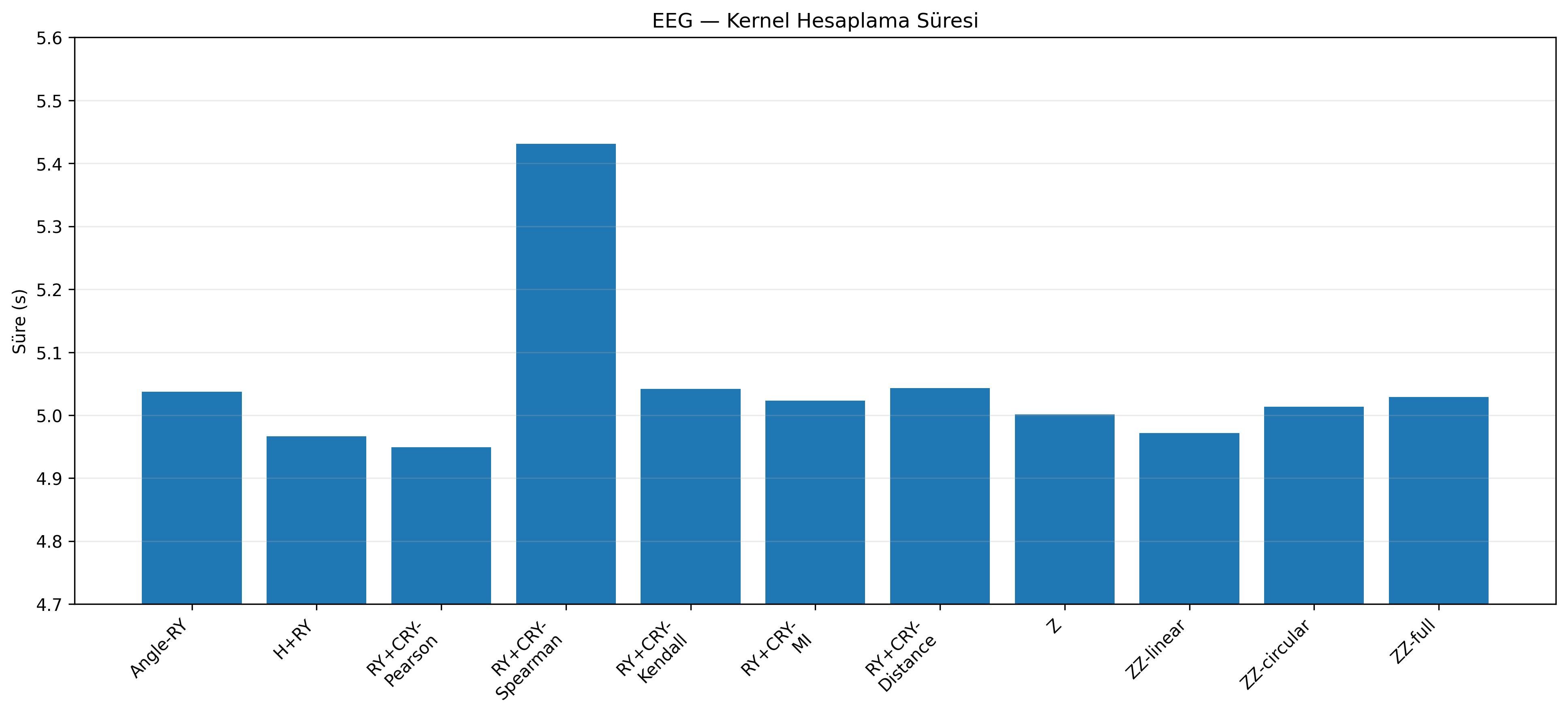
In contrast, Fig. 10 shows that Kernel Time remained largely constant across the encoding methods, ranging from approximately 4.95 to 5.43 seconds. Despite the substantial differences in circuit complexity, the similar kernel computation times indicate that the main differences in total computational cost did not originate from the kernel calculation stage.

Similarly, QSVM training times remained relatively low for all methods (Fig. 11), ranging from approximately 0.066 to 0.182 seconds. Although the highest value, 0.182 seconds, was observed for ZZ circular, this time is negligible compared with the computational cost of state vector generation.
Taken together, these results indicate that the differences in computational cost among the encoding methods arise primarily from quantum-state preparation and state vector computation rather than from classical SVM optimization.
3.1.5 Overall Evaluation of the EEG Dataset
The experiments on the EEG dataset demonstrate that the quantum feature encoding strategy can substantially affect QSVM classification performance. ZZ full achieved the highest test performance, with a Test Accuracy of 0.850, an F1 score of 0.817, and a ROC-AUC of 0.928. However, the same method also exhibited a training accuracy of 1.000, an Accuracy Gap of approximately 0.150, 301 logical gates, a circuit depth of 77, and a state vector computation time of 126.6 seconds. Thus, the maximum test performance was achieved at the cost of high circuit and computational complexity, together with a pronounced training–test gap.
ZZ circular achieved nearly equivalent test performance, with a Test Accuracy of 0.846 and a ROC-AUC of 0.927, while requiring only 70 logical gates and approximately 28 seconds of state vector computation. Therefore, for the EEG dataset, ZZ circular can be regarded as a more efficient alternative to ZZ full in terms of the trade-off between classification performance and circuit complexity.
Z feature Map is particularly notable for its substantially lower circuit complexity. With only 28 logical gates and a circuit depth of 2, it achieved a Test Accuracy of 0.834, an F1 score of 0.802, and a ROC-AUC of 0.910. Furthermore, its Accuracy Gap of 0.060 indicates that Z feature Map provides a strong balance among classification performance, generalization, and circuit cost.
The RY+CRY results demonstrate that incorporating statistical relationships between features into quantum encoding can provide a meaningful performance improvement over Angle-RY. With Pearson-based RY+CRY, test accuracy increased from 0.748 to 0.806. However, representing all 91 feature pairs with CRY gates resulted in 182 CX gates and a decomposed circuit depth of 89.
This observation suggests that, although statistical dependency information can be beneficial, transferring all pairwise relationships into the quantum circuit may not be optimal from an efficiency perspective. Sparser structures in which only the strongest or most meaningful feature relationships are encoded using CRY gates may represent a promising direction for reducing circuit depth and the number of entangling gates while preserving the performance advantage of the RY+CRY approach.
Overall, the EEG experiments show that more complex quantum feature maps can generally provide higher classification performance; however, as connectivity density increases, the marginal performance gain may become increasingly limited while circuit complexity and computational cost rise rapidly. Therefore, the evaluation of quantum feature encoding strategies should not focus exclusively on maximum classification accuracy, but rather on the overall balance among classification performance, generalization behavior, and quantum circuit cost.
3.2 Heart Failure Prediction Dataset
The experiments conducted on the Heart Failure Prediction Dataset compared Angle-RY, H+RY, RY+CRY encodings based on different statistical dependency measures, Z feature Map, and ZZ feature Map with different entanglement structures. The evaluation was performed in terms of classification performance, generalization behavior, quantum circuit complexity, and computational cost.
3.2.1 Classification Performance
| Encoding | Train Acc. | Test Acc. | Acc. Gap | Test Prec. | Test Rec. | Test F1 | Test AUC |
| Angle-RY | 0.903 | 0.874 | 0.029 | 0.850 | 0.937 | 0.891 | 0.909 |
| H+RY | 0.903 | 0.874 | 0.029 | 0.850 | 0.937 | 0.891 | 0.909 |
| RY+CRY-Pearson | 0.914 | 0.883 | 0.032 | 0.873 | 0.921 | 0.897 | 0.927 |
| RY+CRY-Spearman | 0.914 | 0.878 | 0.036 | 0.867 | 0.921 | 0.893 | 0.928 |
| RY+CRY-Kendall | 0.910 | 0.878 | 0.032 | 0.867 | 0.921 | 0.893 | 0.925 |
| RY+CRY-MI | 0.919 | 0.874 | 0.045 | 0.866 | 0.913 | 0.889 | 0.930 |
| RY+CRY-Distance | 0.916 | 0.883 | 0.033 | 0.873 | 0.921 | 0.897 | 0.929 |
| Z | 0.894 | 0.878 | 0.016 | 0.851 | 0.945 | 0.896 | 0.919 |
| ZZ linear | 0.991 | 0.804 | 0.187 | 0.781 | 0.898 | 0.835 | 0.887 |
| ZZ circular | 0.994 | 0.757 | 0.238 | 0.726 | 0.898 | 0.803 | 0.856 |
| ZZ full | 1.000 | 0.843 | 0.157 | 0.810 | 0.937 | 0.869 | 0.911 |

Table 5 and Fig. 12 show that the highest test accuracy for the Heart Failure Prediction Dataset was obtained with the Pearson- and Distance Correlation-based RY+CRY encodings, both achieving 0.883. These methods were followed by Spearman, Kendall, and Z feature Map, each achieving a test accuracy of 0.878. Angle-RY and H+RY both achieved a test accuracy of 0.874.
Compared with Angle-RY, the absolute increase in test accuracy obtained by the Pearson- and Distance Correlation-based RY+CRY encodings was
| (14) |
corresponding to approximately 0.9 percentage points. Therefore, encoding inter-feature relationships through CRY gates improved performance over the basic RY encoding for this dataset, although the improvement was more limited than that observed for the EEG dataset.
It is also noteworthy that H+RY produced exactly the same training and test performance as Angle-RY. Although the addition of the Hadamard layer increased circuit complexity, it did not provide a measurable improvement in classification performance in the present experiment.
A different behavior was observed for the ZZ-based feature maps. Although the training accuracies reached 0.991 for ZZ linear, 0.994 for ZZ circular, and 1.000 for ZZ full, their test accuracies decreased to 0.804, 0.757, and 0.843, respectively. These results indicate that denser ZZ connectivity did not directly translate into improved test performance for the Heart Failure Prediction Dataset.

Figure 13 presents the Precision, Recall, and F1 results together. The highest F1 score, 0.897, was obtained with the Pearson- and Distance Correlation-based RY+CRY encodings. Z feature Map produced a very similar result, with an F1 score of 0.896.
Z feature Map achieved a Recall of 0.945, the highest test Recall among all methods. In contrast, the Pearson- and Distance Correlation-based RY+CRY methods exhibited a more balanced distribution, with a Precision of 0.873 and a Recall of 0.921, resulting in an F1 score of 0.897.
The decrease in the Precision of ZZ circular to 0.726 and its F1 score to 0.803 indicates that the very high performance obtained on the training set was not transferred to the test set to the same extent.

In terms of ROC-AUC, the highest value of 0.930 was obtained with the MI-based RY+CRY encoding. Distance Correlation, Spearman, and Pearson closely followed with values of 0.929, 0.928, and 0.927, respectively.
This result is noteworthy because MI achieved the highest ROC-AUC while its test accuracy of 0.874 remained below those of Pearson and Distance Correlation. Thus, different performance metrics may emphasize different aspects of the quantum feature maps.
ZZ linear and particularly ZZ circular remained behind the other methods, with ROC-AUC values of 0.887 and 0.856, respectively. Therefore, denser ZZ connectivity did not result in greater class-separation capability for this dataset.
3.2.2 Generalization Behavior and Log-Loss
| Encoding | Acc. Gap | Prec. Gap | Recall Gap | F1 Gap | AUC Gap | Train Loss | Test Loss |
| Angle-RY | 0.029 | 0.031 | 0.016 | 0.024 | 0.061 | 0.251 | 0.345 |
| H+RY | 0.029 | 0.031 | 0.016 | 0.024 | 0.061 | 0.251 | 0.345 |
| RY+CRY-Pearson | 0.032 | 0.021 | 0.037 | 0.029 | 0.049 | 0.231 | 0.319 |
| RY+CRY-Spearman | 0.036 | 0.028 | 0.037 | 0.032 | 0.048 | 0.232 | 0.319 |
| RY+CRY-Kendall | 0.032 | 0.021 | 0.037 | 0.029 | 0.050 | 0.237 | 0.321 |
| RY+CRY-MI | 0.045 | 0.034 | 0.047 | 0.040 | 0.047 | 0.227 | 0.317 |
| RY+CRY-Distance | 0.033 | 0.022 | 0.039 | 0.030 | 0.046 | 0.228 | 0.316 |
| Z | 0.016 | 0.026 | -0.005 | 0.012 | 0.047 | 0.273 | 0.345 |
| ZZ linear | 0.187 | 0.204 | 0.102 | 0.157 | 0.112 | 0.047 | 0.425 |
| ZZ circular | 0.238 | 0.263 | 0.102 | 0.192 | 0.144 | 0.031 | 0.472 |
| ZZ full | 0.157 | 0.190 | 0.063 | 0.131 | 0.089 | 0.001 | 0.372 |

Figure 15 clearly illustrates the generalization behavior of the different methods. The lowest Accuracy Gap, 0.016, was obtained with Z feature Map. The corresponding value was 0.029 for Angle-RY and H+RY, whereas the RY+CRY methods remained within the range of approximately 0.032–0.045.
These results indicate relatively small differences between the training and test performance of the RY+CRY methods. In particular, Pearson and Distance Correlation produced the highest test accuracies while maintaining Accuracy Gap values of approximately 0.03. Therefore, the performance improvement achieved by the RY+CRY methods was not accompanied by a pronounced loss of generalization.
In contrast, the Accuracy Gap values for ZZ linear, ZZ circular, and ZZ full were 0.187, 0.238, and 0.157, respectively. The largest gap was observed for ZZ circular. Its training accuracy of 0.994 decreased to a test accuracy of 0.757, indicating a pronounced separation between training and test performance.

The Log-Loss results support the findings obtained from the Accuracy Gap. RY+CRY-Distance Correlation achieved the lowest Test Log-Loss of 0.316, while MI, Pearson, and Spearman produced very similar values of 0.317, 0.319, and 0.319, respectively.
In contrast, although the Train Log-Loss values for ZZ linear and ZZ circular were only 0.047 and 0.031, respectively, their Test Log-Loss values increased to 0.425 and 0.472. In particular, ZZ circular produced the highest test loss among all methods despite its very low training loss, clearly demonstrating the divergence between its training and test behavior.
For ZZ full, the Train Log-Loss was only 0.001, whereas the Test Log-Loss was 0.372. Therefore, for all three ZZ-based methods, the very strong fit to the training data was not transferred to test performance to the same extent.
3.2.3 Quantum Circuit Complexity
| Encoding | H | RY | CRY | CX | Total Gates | Depth | Dec. CX | Dec. Gates | Dec. Depth |
| Angle-RY | 0 | 11 | 0 | 0 | 11 | 1 | 0 | 11 | 1 |
| H+RY | 11 | 11 | 0 | 0 | 22 | 2 | 0 | 22 | 2 |
| RY+CRY-Pearson | 0 | 11 | 55 | 0 | 66 | 20 | 110 | 231 | 68 |
| RY+CRY-Spearman | 0 | 11 | 55 | 0 | 66 | 20 | 110 | 231 | 68 |
| RY+CRY-Kendall | 0 | 11 | 55 | 0 | 66 | 20 | 110 | 231 | 68 |
| RY+CRY-MI | 0 | 11 | 55 | 0 | 66 | 20 | 110 | 231 | 68 |
| RY+CRY-Distance | 0 | 11 | 55 | 0 | 66 | 20 | 110 | 231 | 68 |
| Z | 11 | 0 | 0 | 0 | 22 | 2 | 0 | 22 | 2 |
| ZZ linear | 11 | 0 | 0 | 20 | 52 | 32 | 20 | 52 | 32 |
| ZZ circular | 11 | 0 | 0 | 22 | 55 | 35 | 22 | 55 | 35 |
| ZZ full | 11 | 0 | 0 | 110 | 187 | 59 | 110 | 187 | 59 |


Since 11 features were used for the Heart Failure Prediction Dataset, the basic RY-based encoding consists of 11 RY gates. The number of all unique feature pairs is
| (15) |
Therefore, each RY+CRY method contains 55 CRY gates. These circuits have a total logical gate count of 66 and a circuit depth of 20.
It is important to note that the Pearson, Spearman, Kendall, MI, and Distance Correlation methods have identical circuit complexities. Consequently, differences in classification performance among these methods do not arise from circuit size but from the statistical dependency values used to determine the CRY rotation angles.
Z feature Map achieved a test accuracy of 0.878 with only 22 gates and a circuit depth of 2. This makes Z feature Map a particularly efficient option in terms of circuit cost for the Heart Failure Prediction Dataset.

As the density of ZZ connectivity increases, the number of CX gates also increases substantially. ZZ linear, ZZ circular, and ZZ full contain 20, 22, and 110 CX gates, respectively. Nevertheless, the test accuracy of ZZ full was only 0.843, remaining below the results obtained with RY+CRY and Z feature Map.
This finding is important for the Heart Failure Prediction Dataset: a denser entanglement structure alone does not guarantee higher classification performance. The compatibility between the structure of the feature space and the selected entanglement topology appears to be more important than the number of entangling gates alone.

After decomposition, the RY+CRY circuits contain 231 total gates, 110 CX gates, and a circuit depth of 68. These values indicate a substantial circuit cost compared with Angle-RY and Z feature Map.
Nevertheless, the fact that the Pearson- and Distance Correlation-based RY+CRY methods achieved the highest test accuracy of 0.883 indicates that incorporating dependency information into quantum encoding can be beneficial for classification performance. However, an accuracy improvement of approximately 0.9 percentage points requires 231 decomposed gates and 110 CX gates, emphasizing the need to evaluate the trade-off between performance and circuit cost.
3.2.4 Computational Cost
| Encoding | State vector Time | Kernel Time | Training Time |
| Angle-RY | 1.044 | 0.1510 | 0.0208 |
| H+RY | 1.757 | 0.1500 | 0.0194 |
| RY+CRY-Pearson | 6.594 | 0.1524 | 0.0200 |
| RY+CRY-Spearman | 6.549 | 0.1515 | 0.0208 |
| RY+CRY-Kendall | 6.702 | 0.1525 | 0.0206 |
| RY+CRY-MI | 6.668 | 0.1509 | 0.0207 |
| RY+CRY-Distance | 6.939 | 0.1521 | 0.0213 |
| Z | 1.910 | 0.1518 | 0.0228 |
| ZZ linear | 3.837 | 0.1495 | 0.0314 |
| ZZ circular | 4.173 | 0.1525 | 0.0324 |
| ZZ full | 13.633 | 0.1510 | 0.0311 |

The computation times generally follow the differences in circuit complexity. Angle-RY had the lowest state vector computation time at approximately 1.04 seconds, whereas the corresponding value for Z feature Map was approximately 1.91 seconds.
The state vector computation times of the RY+CRY methods ranged from approximately 6.55 to 6.94 seconds. The similarity of these values is consistent with the identical circuit topology used by these methods.
The highest state vector computation time, 13.63 seconds, was obtained with ZZ full. Compared with Angle-RY, this corresponds to approximately
| (16) |
times higher computational cost. Nevertheless, because the test accuracy of ZZ full was lower than that of Angle-RY, the increased circuit cost did not translate into improved performance for this dataset.
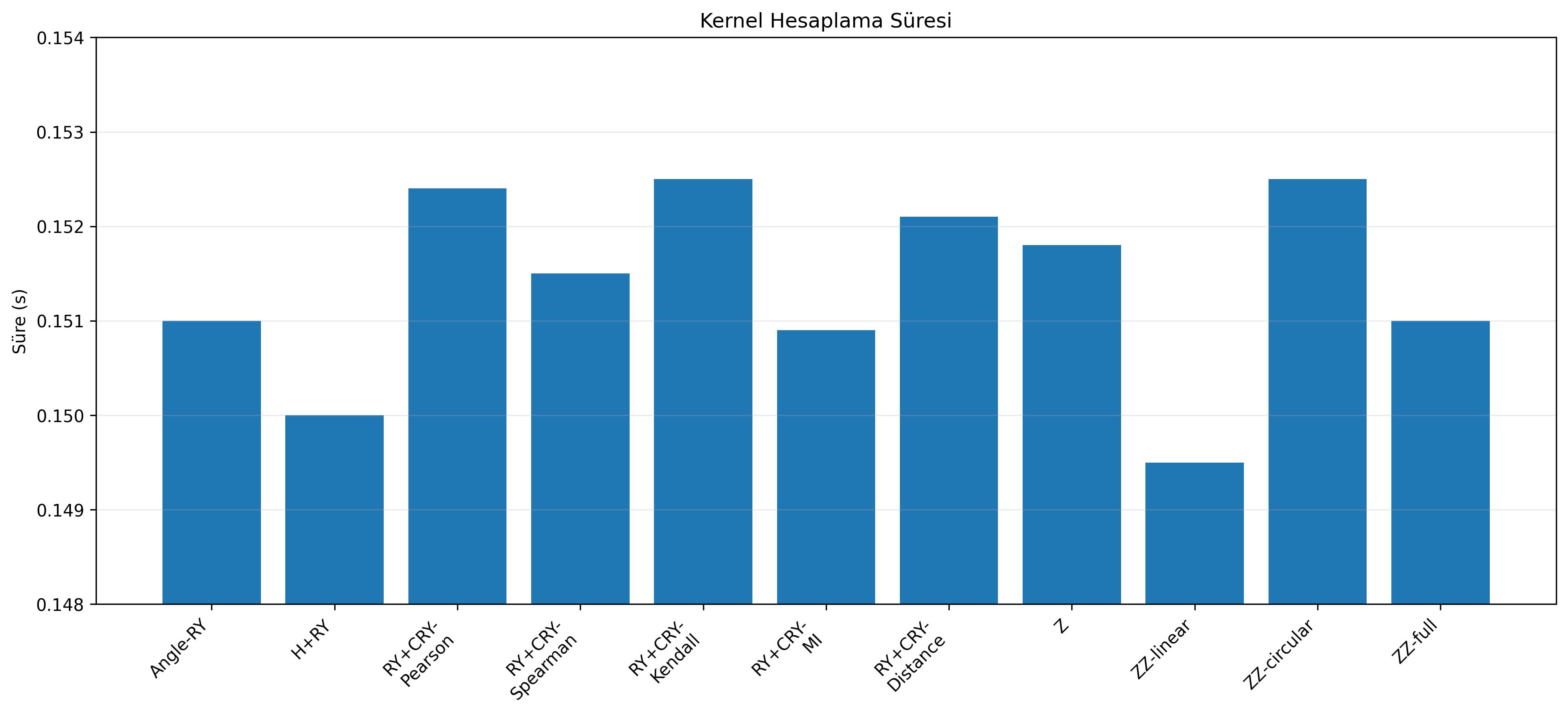
Kernel computation times remained highly stable across the methods, ranging from approximately 0.150 to 0.153 seconds. Despite substantial differences in circuit complexity, the similar kernel times indicate that the main differences in total computational cost did not originate from the kernel computation stage.

QSVM training times were also very low for all methods. The training time was approximately 0.021 seconds for Angle-RY and approximately 0.031–0.032 seconds for ZZ linear, ZZ circular, and ZZ full.
Therefore, the primary source of the computational cost differences among the methods in the Heart Failure Prediction experiments was the preparation of quantum states and state vector computation rather than the classical SVM training stage.
3.2.5 Overall Evaluation of the Heart Failure Prediction Dataset
The results obtained for the Heart Failure Prediction Dataset clearly show that more complex quantum feature maps do not necessarily provide higher classification performance. The highest test accuracy, 0.883, was achieved with the Pearson- and Distance Correlation-based RY+CRY encodings. These methods also exhibited relatively balanced training and test behavior, with Accuracy Gap values of approximately 0.03.
Z feature Map is particularly noteworthy in terms of the performance–complexity trade-off. With only 22 logical gates and a circuit depth of 2, it achieved a test accuracy of 0.878, an F1 score of 0.896, and a ROC-AUC of 0.919. Furthermore, it produced the lowest Accuracy Gap among all methods, at 0.016. Therefore, when maximum test accuracy is not the sole objective, Z feature Map can be considered a highly efficient option for the Heart Failure Prediction Dataset.
The RY+CRY methods provided a limited but consistent improvement over Angle-RY. In particular, Pearson and Distance Correlation achieved the highest test accuracy. However, encoding all 55 feature pairs using CRY gates resulted in 231 gates, 110 CX gates, and a decomposed circuit depth of 68. Therefore, the observed performance improvement should be evaluated together with the associated circuit cost.
The most pronounced behavior was observed for the ZZ-based feature maps. Although these methods achieved nearly perfect performance on the training set, their test performance decreased substantially and the training–test gaps increased. In particular, ZZ circular achieved a training accuracy of 0.994 but only a test accuracy of 0.757, resulting in an Accuracy Gap of 0.238.
Overall, the Heart Failure Prediction experiments demonstrate that the effectiveness of a quantum feature encoding strategy is not determined solely by the density of circuit connectivity. Greater entanglement and more complex feature maps may fail to produce higher classification performance when they are not well matched to the underlying data structure. Therefore, the evaluation of feature encoding strategies for QSVM should jointly consider test performance, generalization behavior, and quantum circuit complexity.
3.3 Credit Risk Dataset
The experiments conducted on the Credit Risk Dataset compared Angle-RY, H+RY, RY+CRY encodings based on different statistical dependency measures, Z feature Map, and ZZ feature Map with linear, circular, and full entanglement structures. The evaluation was performed in terms of classification performance, generalization behavior, quantum circuit complexity, and computational cost.
3.3.1 Classification Performance
| Encoding | Train Acc. | Test Acc. | Acc. Gap | Test Prec. | Test Rec. | Test F1 | Test AUC |
| Angle-RY | 0.907 | 0.908 | -0.001 | 0.824 | 0.908 | 0.864 | 0.654 |
| H+RY | 0.907 | 0.908 | -0.001 | 0.824 | 0.908 | 0.864 | 0.654 |
| RY+CRY-Pearson | 0.907 | 0.908 | -0.001 | 0.824 | 0.908 | 0.864 | 0.658 |
| RY+CRY-Spearman | 0.907 | 0.908 | -0.001 | 0.824 | 0.908 | 0.864 | 0.659 |
| RY+CRY-Kendall | 0.907 | 0.908 | -0.001 | 0.824 | 0.908 | 0.864 | 0.654 |
| RY+CRY-MI | 0.907 | 0.908 | -0.001 | 0.824 | 0.908 | 0.864 | 0.654 |
| RY+CRY-Distance | 0.908 | 0.908 | 0.000 | 0.824 | 0.908 | 0.864 | 0.663 |
| Z | 0.915 | 0.908 | 0.007 | 0.824 | 0.908 | 0.864 | 0.464 |
| ZZ linear | 0.933 | 0.908 | 0.025 | 0.824 | 0.908 | 0.864 | 0.619 |
| ZZ circular | 0.933 | 0.908 | 0.025 | 0.824 | 0.908 | 0.864 | 0.606 |
| ZZ full | 0.945 | 0.908 | 0.037 | 0.824 | 0.908 | 0.864 | 0.613 |

Table 9 and Fig. 23 show that all encoding methods produced the same test accuracy (0.908) on the Credit Risk Dataset. Therefore, changing the quantum feature encoding strategy did not alter the final classification accuracy under the decision threshold used in this study.
Differences were nevertheless observed in training accuracy. Angle-RY, H+RY, and the Pearson-, Spearman-, Kendall-, and MI-based RY+CRY methods produced training accuracies of approximately 0.907. The training accuracy increased to 0.915 for Z feature Map, 0.933 for both ZZ linear and ZZ circular, and 0.945 for ZZ full.
These results indicate that more complex feature maps provided a stronger fit to the training data; however, this additional fit did not translate into an improvement in test accuracy.

As shown in Fig. 24, not only Accuracy but also Precision, Recall, and F1 were identical across all methods. Test Precision was 0.824, Recall was 0.908, and F1 was 0.864.
This result highlights an important observation. Although different quantum feature maps may generate different similarity structures in the kernel space, they produced the same class labels under the classification threshold used in this experiment. Consequently, threshold-dependent metrics such as Accuracy, Precision, Recall, and F1 were unable to differentiate the methods in this case.
Therefore, ROC-AUC and probability-based measures such as Log-Loss provide more informative criteria for distinguishing the encoding strategies on this dataset.

Although the test Accuracy was identical across all methods, the ROC-AUC results differed considerably, as illustrated in Fig. 25.
The highest test ROC-AUC, 0.663, was obtained with the Distance Correlation-based RY+CRY encoding. It was followed by Spearman at 0.659 and Pearson at 0.658. Angle-RY and H+RY both produced ROC-AUC values of approximately 0.654.
These results indicate that although the dependency-based controlled rotations did not change the test Accuracy, they could provide a limited improvement in the relative ranking or separability of the classes.
Notably, Z feature Map produced a ROC-AUC of only 0.464. Despite its test accuracy of 0.908, this low value indicates weak class discrimination in terms of the underlying decision scores.
The ROC-AUC values for ZZ linear, ZZ circular, and ZZ full were 0.619, 0.606, and 0.613, respectively. Thus, the higher circuit complexity of these feature maps did not provide an advantage in terms of ROC-AUC.
3.3.2 Generalization Behavior and Log-Loss
| Encoding | Acc. Gap | Prec. Gap | Recall Gap | F1 Gap | AUC Gap | Train Loss | Test Loss |
| Angle-RY | -0.001 | -0.002 | -0.001 | -0.002 | -0.109 | 0.365 | 0.361 |
| H+RY | -0.001 | -0.002 | -0.001 | -0.002 | -0.109 | 0.365 | 0.361 |
| RY+CRY-Pearson | -0.001 | -0.002 | -0.001 | -0.002 | -0.118 | 0.368 | 0.363 |
| RY+CRY-Spearman | -0.001 | -0.002 | -0.001 | -0.002 | -0.119 | 0.367 | 0.363 |
| RY+CRY-Kendall | -0.001 | -0.002 | -0.001 | -0.002 | -0.112 | 0.366 | 0.362 |
| RY+CRY-MI | -0.001 | -0.002 | -0.001 | -0.002 | -0.115 | 0.368 | 0.362 |
| RY+CRY-Distance | 0.000 | 0.040 | 0.000 | 0.001 | -0.130 | 0.373 | 0.363 |
| Z | 0.007 | 0.098 | 0.007 | 0.016 | -0.154 | 0.414 | 0.373 |
| ZZ linear | 0.025 | 0.113 | 0.025 | 0.052 | 0.369 | 0.282 | 0.369 |
| ZZ circular | 0.025 | 0.113 | 0.025 | 0.052 | 0.353 | 0.283 | 0.370 |
| ZZ full | 0.037 | 0.124 | 0.037 | 0.071 | -0.056 | 0.341 | 0.369 |

Figure 26 demonstrates differences in generalization behavior among the methods. For Angle-RY, H+RY, and the first four RY+CRY methods, the Accuracy Gap was approximately -0.001. This small negative value indicates that test accuracy was approximately 0.001 higher than training accuracy and, in practical terms, shows that training and test performance were nearly identical.
For the Distance Correlation-based RY+CRY encoding, the training and test accuracies were identical, resulting in an Accuracy Gap of zero.
The gap increased to 0.007 for Z feature Map, 0.025 for ZZ linear and ZZ circular, and 0.037 for ZZ full. Nevertheless, these values remain considerably smaller than the large generalization gaps observed for the ZZ-based methods on some of the other datasets.
The important observation is that training accuracy increased with circuit complexity, whereas test accuracy remained fixed at 0.908. Thus, the additional fit of the ZZ encodings to the training data did not improve test performance on this dataset.

The Log-Loss results reveal differences among the methods that are not apparent from Accuracy alone.
The Test Log-Loss was approximately 0.361 for Angle-RY and H+RY. For the RY+CRY methods, the values were very similar and ranged from approximately 0.362 to 0.363.
Z feature Map produced a higher Test Log-Loss of 0.373. The corresponding values for ZZ linear, ZZ circular, and ZZ full were 0.369, 0.370, and 0.369, respectively.
In particular, although the Train Log-Loss values of ZZ linear and ZZ circular decreased to approximately 0.282, their Test Log-Loss remained close to 0.370. This indicates that the stronger fit obtained on the training data was not transferred to the test data to the same extent.
Therefore, although Accuracy was identical for all methods on the Credit Risk Dataset, the Log-Loss and ROC-AUC results reveal meaningful differences among the quantum feature maps.
3.3.3 Quantum Circuit Complexity
| Encoding | H | RY | CRY | CX | Total Gates | Depth | Dec. CX | Dec. Gates | Dec. Depth |
| Angle-RY | 0 | 9 | 0 | 0 | 9 | 1 | 0 | 9 | 1 |
| H+RY | 9 | 9 | 0 | 0 | 18 | 2 | 0 | 18 | 2 |
| RY+CRY-Pearson | 0 | 9 | 36 | 0 | 45 | 16 | 72 | 153 | 54 |
| RY+CRY-Spearman | 0 | 9 | 36 | 0 | 45 | 16 | 72 | 153 | 54 |
| RY+CRY-Kendall | 0 | 9 | 36 | 0 | 45 | 16 | 72 | 153 | 54 |
| RY+CRY-MI | 0 | 9 | 36 | 0 | 45 | 16 | 72 | 153 | 54 |
| RY+CRY-Distance | 0 | 9 | 36 | 0 | 45 | 16 | 72 | 153 | 54 |
| Z | 9 | 0 | 0 | 0 | 18 | 2 | 0 | 18 | 2 |
| ZZ linear | 9 | 0 | 0 | 16 | 42 | 26 | 16 | 42 | 26 |
| ZZ circular | 9 | 0 | 0 | 18 | 45 | 29 | 18 | 45 | 29 |
| ZZ full | 9 | 0 | 0 | 72 | 126 | 47 | 72 | 126 | 47 |


Nine features were used in the Credit Risk experiment. Therefore, the Angle-RY encoding consists of nine RY gates, while the number of all possible pairwise feature relationships is
| (17) |
Consequently, each RY+CRY method contains 36 CRY gates.
The RY+CRY circuits have a total logical gate count of 45 and a circuit depth of 16. Since the circuit structure is identical for all five dependency measures, the differences in ROC-AUC cannot be attributed to circuit size but instead arise from the dependency measures used to determine the CRY rotation angles.
Z feature Map achieved the same test accuracy of 0.908 with only 18 logical gates and a circuit depth of 2. However, its low ROC-AUC demonstrates that an evaluation based solely on Accuracy could overlook important differences between the methods.

In terms of entangling gates, the RY+CRY methods contain 36 logical CRY operations, which result in 72 CX gates after decomposition.
The numbers of CX gates for ZZ linear, ZZ circular, and ZZ full are 16, 18, and 72, respectively. Nevertheless, all three methods achieved the same test accuracy of 0.908.
This result clearly demonstrates that increasing entanglement density did not provide an additional improvement in classification accuracy on the Credit Risk Dataset.

After decomposition, the RY+CRY circuits contain 153 total gates, 72 CX gates, and a circuit depth of 54. In contrast, Angle-RY contains only 9 gates and has a circuit depth of 1.
Despite this substantial increase in circuit complexity, Angle-RY and the RY+CRY methods achieved identical test accuracies. Therefore, the increase in circuit complexity did not translate into an improvement in threshold-dependent classification performance for this dataset.
The potential advantage of RY+CRY is more apparent in the ROC-AUC results. For example, the ROC-AUC increased from 0.654 for Angle-RY to 0.663 for the Distance Correlation-based RY+CRY method. However, this limited improvement should be considered together with the cost of 153 decomposed gates and 72 CX gates.
ZZ full is the most complex ZZ-based structure, with 126 logical gates, 72 CX gates, and a circuit depth of 47. Nevertheless, its test Accuracy, Precision, Recall, and F1 values were identical to those obtained with the simplest Angle-RY encoding.
3.3.4 Computational Cost
| Encoding | state vector Time | Kernel Time | Training Time |
| Angle-RY | 0.774 | 0.0547 | 0.0234 |
| H+RY | 1.254 | 0.0546 | 0.0231 |
| RY+CRY-Pearson | 3.761 | 0.0538 | 0.0238 |
| RY+CRY-Spearman | 3.935 | 0.0543 | 0.0235 |
| RY+CRY-Kendall | 4.072 | 0.0554 | 0.0235 |
| RY+CRY-MI | 4.033 | 0.0540 | 0.0236 |
| RY+CRY-Distance | 3.652 | 0.0607 | 0.0247 |
| Z | 1.403 | 0.0540 | 0.0268 |
| ZZ linear | 2.768 | 0.0547 | 0.0425 |
| ZZ circular | 2.899 | 0.0547 | 0.0442 |
| ZZ full | 7.396 | 0.0548 | 0.0493 |

The state vector computation time generally followed the circuit complexity. The lowest computation time, 0.774 seconds, was obtained with Angle-RY. H+RY and Z feature Map required approximately 1.25 and 1.40 seconds, respectively.
The state vector computation times of the RY+CRY methods ranged from approximately 3.65 to 4.07 seconds, whereas ZZ full had the highest state vector cost at 7.40 seconds.
The state vector computational cost of ZZ full relative to Angle-RY was approximately
| (18) |
Thus, ZZ full required approximately 9.6 times more state vector computation time than Angle-RY. Nevertheless, the two methods produced identical test Accuracy, Precision, Recall, and F1 values. This result strongly indicates that the increase in circuit complexity did not directly translate into improved classification output for the Credit Risk Dataset.
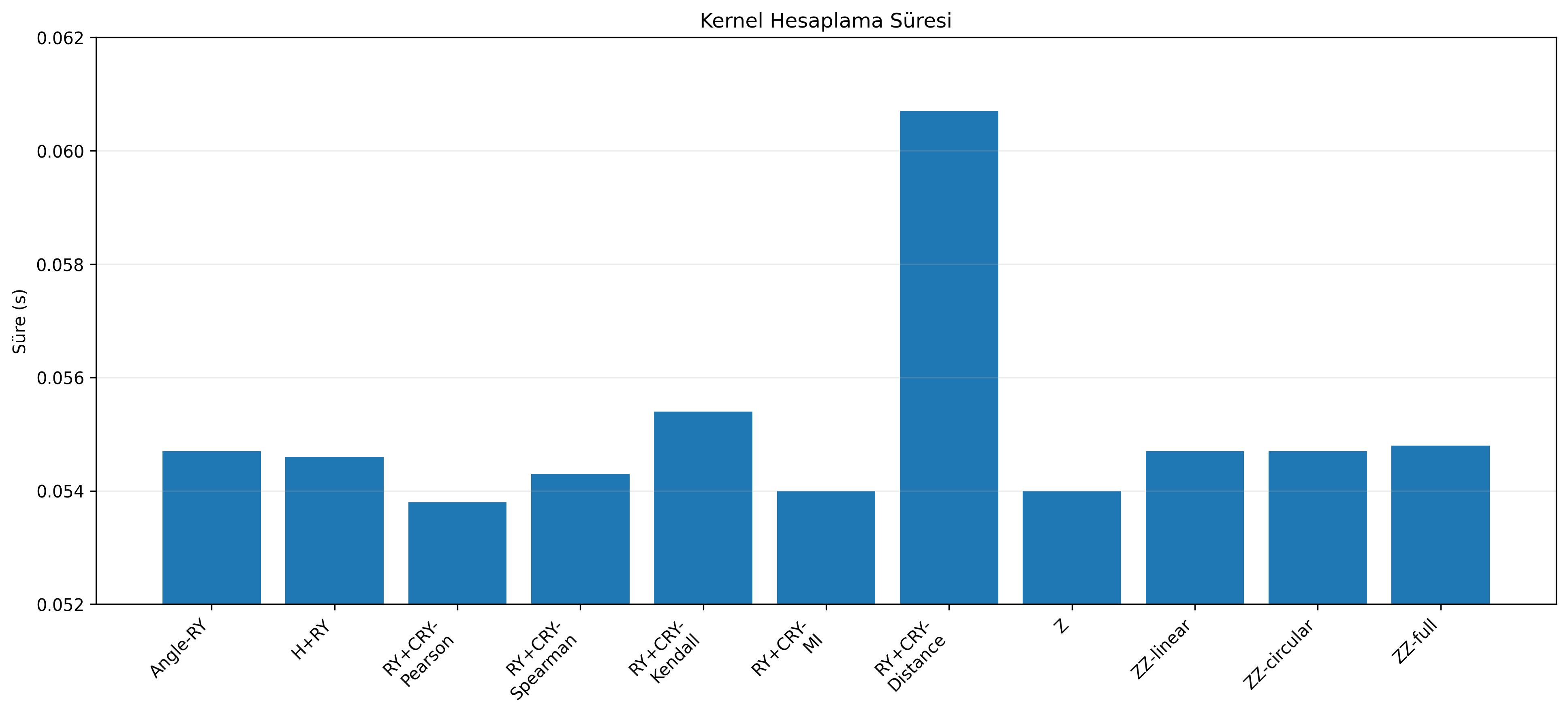
Kernel computation times generally remained within approximately 0.054–0.055 seconds. Although a value of approximately 0.061 seconds was observed for the Distance Correlation-based RY+CRY method, the differences among the methods were generally small.
This result indicates that the differences in total computational cost primarily arose during quantum-state preparation rather than from the subsequent processing of the kernel matrix.

The training times for Angle-RY and the RY+CRY methods were approximately 0.023–0.025 seconds. They increased to approximately 0.043–0.044 seconds for ZZ linear and ZZ circular and to approximately 0.049 seconds for ZZ full.
Nevertheless, all training times were substantially smaller than the state vector computation times. Therefore, the primary source of the computational cost differences among the methods was again the preparation of the quantum feature states.
3.3.5 Overall Evaluation of the Credit Risk Dataset
The Credit Risk Dataset exhibited a different behavior from the other datasets. All quantum feature encoding strategies produced the same test Accuracy of 0.908, Precision of 0.824, Recall of 0.908, and F1 score of 0.864. Therefore, when only these metrics are considered, no performance difference among the methods is observed.
However, the ROC-AUC results demonstrate that the quantum feature maps are not entirely equivalent. The highest ROC-AUC, 0.663, was obtained with the Distance Correlation-based RY+CRY method, whereas Z feature Map produced only 0.464. Thus, despite identical final classification accuracy, the ranking of samples according to their decision scores may differ substantially.
In terms of generalization, the training–test accuracy gaps for Angle-RY and the RY+CRY methods were nearly zero. In contrast, as the ZZ connectivity density increased, training accuracy improved while test accuracy remained unchanged. This indicates that greater feature-map complexity improved the fit to the training data without providing an additional benefit in generalization performance.
A similar conclusion can be drawn from circuit cost. Angle-RY achieved a test accuracy of 0.908 using only 9 logical gates and a circuit depth of 1, whereas ZZ full produced the same test accuracy using 126 gates and a circuit depth of 47. The state vector computation time also increased from approximately 0.77 seconds to 7.40 seconds.
Therefore, the use of more complex encodings does not provide a clear advantage in terms of threshold-dependent classification performance for the Credit Risk Dataset. The limited advantage of the RY+CRY methods is primarily observed in threshold-independent discrimination metrics such as ROC-AUC.
Overall, the Credit Risk experiments demonstrate that higher circuit complexity does not necessarily translate into higher classification performance for every dataset. For this dataset in particular, quantum feature encoding strategies should be evaluated not only in terms of Accuracy but also by jointly considering ROC-AUC, Log-Loss, generalization gap, and circuit cost.
3.4 Student Performance Dataset
The experiments conducted on the Student Performance Dataset compared Angle-RY, H+RY, RY+CRY encodings based on different statistical dependency measures, Z feature Map, and ZZ feature Map with different entanglement structures. The evaluation was performed in terms of classification performance, generalization behavior, quantum circuit complexity, and computational cost.
3.4.1 Classification Performance
| Encoding | Train Acc. | Test Acc. | Acc. Gap | Test Prec. | Test Rec. | Test F1 | Test AUC |
| Angle-RY | 0.995 | 0.882 | 0.113 | 0.900 | 0.673 | 0.770 | 0.953 |
| H+RY | 0.995 | 0.882 | 0.113 | 0.900 | 0.673 | 0.770 | 0.953 |
| RY+CRY-Pearson | 0.998 | 0.890 | 0.108 | 0.918 | 0.687 | 0.786 | 0.962 |
| RY+CRY-Spearman | 0.998 | 0.890 | 0.108 | 0.918 | 0.687 | 0.786 | 0.962 |
| RY+CRY-Kendall | 0.997 | 0.890 | 0.107 | 0.918 | 0.687 | 0.786 | 0.961 |
| RY+CRY-MI | 0.997 | 0.886 | 0.111 | 0.902 | 0.687 | 0.780 | 0.960 |
| RY+CRY-Distance | 0.998 | 0.890 | 0.108 | 0.918 | 0.687 | 0.786 | 0.963 |
| Z | 0.968 | 0.944 | 0.024 | 0.947 | 0.857 | 0.900 | 0.975 |
| ZZ linear | 0.997 | 0.908 | 0.089 | 0.932 | 0.741 | 0.826 | 0.960 |
| ZZ circular | 0.996 | 0.888 | 0.108 | 0.925 | 0.673 | 0.780 | 0.948 |
| ZZ full | 1.000 | 0.712 | 0.288 | 1.000 | 0.020 | 0.040 | 0.909 |

Table 13 and Fig. 34 show that the highest test accuracy on the Student Performance Dataset was obtained with Z feature Map, which achieved 0.944. ZZ linear produced the second-highest test accuracy at 0.908, whereas the Pearson-, Spearman-, Kendall-, and Distance Correlation-based RY+CRY methods achieved 0.890.
Angle-RY and H+RY both achieved a test accuracy of 0.882. Although the improvement provided by the RY+CRY encodings over this baseline was limited, it was consistent. For example, the absolute increase in accuracy for the Pearson-based RY+CRY method was
| (19) |
corresponding to approximately 0.8 percentage points.
In contrast, the improvement of Z feature Map over Angle-RY was
| (20) |
corresponding to approximately 6.2 percentage points. This result suggests that the Z-based feature map provides a representation better suited to the structure of the Student Performance Dataset than the other investigated encodings.
ZZ full, however, achieved a training accuracy of 1.000 while its test accuracy decreased to only 0.712. This clearly demonstrates that greater model complexity does not guarantee improved test performance.

Figure 35 further highlights the superior performance of Z feature Map. It achieved a Precision of 0.947, Recall of 0.857, and F1 score of 0.900, providing the most balanced test performance among all methods.
The Pearson-, Spearman-, Kendall-, and Distance Correlation-based RY+CRY methods achieved a Precision of 0.918, Recall of 0.687, and an F1 score of approximately 0.786. Although Precision remained high for these methods, their lower Recall values reduced the overall F1 score.
ZZ linear achieved a Precision of 0.932 and a Recall of 0.741, resulting in an F1 score of 0.826. This performance exceeded that of the RY+CRY methods, but remained below the F1 score of 0.900 obtained with Z feature Map.
The most striking result was observed for ZZ full. Although its Precision reached 1.000, its Recall was only 0.020, resulting in an F1 score of 0.040. Thus, while ZZ full was highly accurate for the very small number of samples it predicted as positive, it failed to identify nearly all actual positive samples.

The ROC-AUC results also support the superiority of Z feature Map. The highest test ROC-AUC value, 0.975, was obtained with Z feature Map.
Among the RY+CRY methods, Distance Correlation achieved the highest ROC-AUC at 0.963, followed closely by Pearson and Spearman at approximately 0.962. This finding indicates that dependency-based CRY rotations can improve class separability relative to Angle-RY to some extent.
ZZ linear achieved a strong ROC-AUC value of 0.960, whereas ZZ circular and ZZ full decreased to 0.948 and 0.909, respectively. Therefore, increasing the connectivity density did not provide a systematic advantage in terms of ROC-AUC for this dataset.
3.4.2 Generalization Behavior and Log-Loss
| Encoding | Acc. Gap | Prec. Gap | Recall Gap | F1 Gap | AUC Gap | Train Loss | Test Loss |
| Angle-RY | 0.113 | 0.093 | 0.318 | 0.222 | 0.047 | 0.022 | 0.260 |
| H+RY | 0.113 | 0.093 | 0.318 | 0.222 | 0.047 | 0.022 | 0.260 |
| RY+CRY-Pearson | 0.108 | 0.080 | 0.308 | 0.211 | 0.038 | 0.013 | 0.236 |
| RY+CRY-Spearman | 0.108 | 0.080 | 0.308 | 0.211 | 0.038 | 0.013 | 0.237 |
| RY+CRY-Kendall | 0.107 | 0.077 | 0.306 | 0.208 | 0.039 | 0.015 | 0.240 |
| RY+CRY-MI | 0.111 | 0.094 | 0.306 | 0.214 | 0.040 | 0.016 | 0.245 |
| RY+CRY-Distance | 0.108 | 0.080 | 0.308 | 0.211 | 0.037 | 0.012 | 0.233 |
| Z | 0.024 | 0.043 | 0.044 | 0.043 | 0.021 | 0.079 | 0.160 |
| ZZ linear | 0.089 | 0.068 | 0.247 | 0.169 | 0.040 | 0.011 | 0.217 |
| ZZ circular | 0.108 | 0.075 | 0.313 | 0.214 | 0.052 | 0.008 | 0.252 |
| ZZ full | 0.288 | 0.000 | 0.980 | 0.960 | 0.091 | 0.001 | 0.349 |

In terms of generalization behavior, Z feature Map produced the most notable result. Its training accuracy was 0.968 and its test accuracy was 0.944, resulting in an Accuracy Gap of only 0.024.
In contrast, Angle-RY and H+RY produced an Accuracy Gap of approximately 0.113, whereas the RY+CRY methods produced values in the range of approximately 0.107–0.111. These methods achieved training accuracies of approximately 0.997–0.998 but remained near 0.89 in test accuracy.
The Accuracy Gap was 0.089 for ZZ linear and increased to 0.108 for ZZ circular. The highest generalization gap, 0.288, was obtained with ZZ full.
Although ZZ full achieved a training accuracy of 1.000, its test accuracy decreased to 0.712, indicating a strong overfitting tendency. This behavior is even more apparent from its Recall Gap of approximately 0.980 and F1 Gap of 0.960.

The Log-Loss results support the generalization analysis. The Test Log-Loss was approximately 0.260 for Angle-RY and H+RY, whereas it decreased to approximately 0.236 for the Pearson- and Spearman-based RY+CRY methods.
RY+CRY-Distance Correlation achieved the lowest test loss within the RY+CRY group, at 0.233. However, the lowest overall Test Log-Loss, 0.160, was obtained with Z feature Map.
The fact that Z feature Map achieved both the highest test accuracy and the lowest Test Log-Loss indicates that it not only predicted class labels more accurately but also produced more reliable prediction confidence.
In contrast, ZZ full achieved a Train Log-Loss of only 0.001 while its Test Log-Loss increased to 0.349. This sharp divergence clearly indicates that the extremely strong fit to the training data did not generalize to the test set.
3.4.3 Quantum Circuit Complexity
| Encoding | H | RY | CRY | CX | Total Gates | Depth | Dec. CX | Dec. Gates | Dec. Depth |
| Angle-RY | 0 | 13 | 0 | 0 | 13 | 1 | 0 | 13 | 1 |
| H+RY | 13 | 13 | 0 | 0 | 26 | 2 | 0 | 26 | 2 |
| RY+CRY-Pearson | 0 | 13 | 78 | 0 | 91 | 24 | 156 | 325 | 82 |
| RY+CRY-Spearman | 0 | 13 | 78 | 0 | 91 | 24 | 156 | 325 | 82 |
| RY+CRY-Kendall | 0 | 13 | 78 | 0 | 91 | 24 | 156 | 325 | 82 |
| RY+CRY-MI | 0 | 13 | 78 | 0 | 91 | 24 | 156 | 325 | 82 |
| RY+CRY-Distance | 0 | 13 | 78 | 0 | 91 | 24 | 156 | 325 | 82 |
| Z | 13 | 0 | 0 | 0 | 26 | 2 | 0 | 26 | 2 |
| ZZ linear | 13 | 0 | 0 | 24 | 62 | 38 | 24 | 62 | 38 |
| ZZ circular | 13 | 0 | 0 | 26 | 65 | 41 | 26 | 65 | 41 |
| ZZ full | 13 | 0 | 0 | 156 | 260 | 71 | 156 | 260 | 71 |


Since 13 features were used in the Student Performance experiment, the Angle-RY circuit consists of 13 RY gates. The number of all unique feature pairs is
| (21) |
Therefore, the RY+CRY methods contain 78 CRY gates.
At the logical level, the RY+CRY methods contain 91 gates and have a circuit depth of 24. After decomposition, the total gate count increases to 325, the number of CX gates to 156, and the circuit depth to 82.
In contrast, Z feature Map achieved the highest test performance among all methods with only 26 logical gates and a circuit depth of 2. This result demonstrates that greater circuit complexity was not required for strong performance on the Student Performance Dataset.

ZZ linear, ZZ circular, and ZZ full contain 24, 26, and 156 CX gates, respectively. Nevertheless, test performance did not systematically improve as connectivity density increased.
In particular, although ZZ full contains 156 CX gates, it achieved only 0.712 test accuracy and an F1 score of 0.040. Thus, the dense entanglement structure did not provide a suitable representation for classification on this dataset.

The decomposed circuit complexity shows that the RY+CRY methods require 325 total gates, 156 CX gates, and a circuit depth of 82. In contrast, Z feature Map requires only 26 total gates and a circuit depth of 2.
The difference in classification performance between these two structures also favors Z feature Map. Z feature Map achieved a Test Accuracy of 0.944 and an F1 score of 0.900, whereas the RY+CRY methods remained at approximately 0.890 Test Accuracy and 0.786 F1.
Therefore, for this dataset, the more complex RY+CRY structure that connects all feature pairs did not provide a performance advantage over the lower-cost Z feature Map.
3.4.4 Computational Cost
| Encoding | state vector Time | Kernel Time | Training Time |
| Angle-RY | 3.584 | 2.480 | 0.135 |
| H+RY | 6.072 | 2.461 | 0.127 |
| RY+CRY-Pearson | 26.061 | 2.457 | 0.134 |
| RY+CRY-Spearman | 26.122 | 2.459 | 0.129 |
| RY+CRY-Kendall | 26.533 | 2.502 | 0.127 |
| RY+CRY-MI | 26.879 | 2.531 | 0.136 |
| RY+CRY-Distance | 26.635 | 2.500 | 0.134 |
| Z | 6.228 | 2.500 | 0.086 |
| ZZ linear | 13.595 | 2.482 | 0.147 |
| ZZ circular | 14.758 | 2.465 | 0.144 |
| ZZ full | 59.357 | 2.470 | 0.137 |

The state vector computation times generally follow the differences in circuit complexity. Angle-RY had the lowest computation time at approximately 3.58 seconds, whereas Z feature Map required approximately 6.23 seconds.
The RY+CRY methods required approximately 26–27 seconds for state vector computation. The highest value, approximately 59.36 seconds, was observed for ZZ full.
The state vector cost of ZZ full relative to Z feature Map was approximately
| (22) |
Thus, although ZZ full required approximately 9.5 times more state vector computation time than Z feature Map, its test accuracy of 0.712 remained far below the 0.944 achieved by Z feature Map. This result demonstrates that higher computational cost did not translate into improved performance for this dataset.
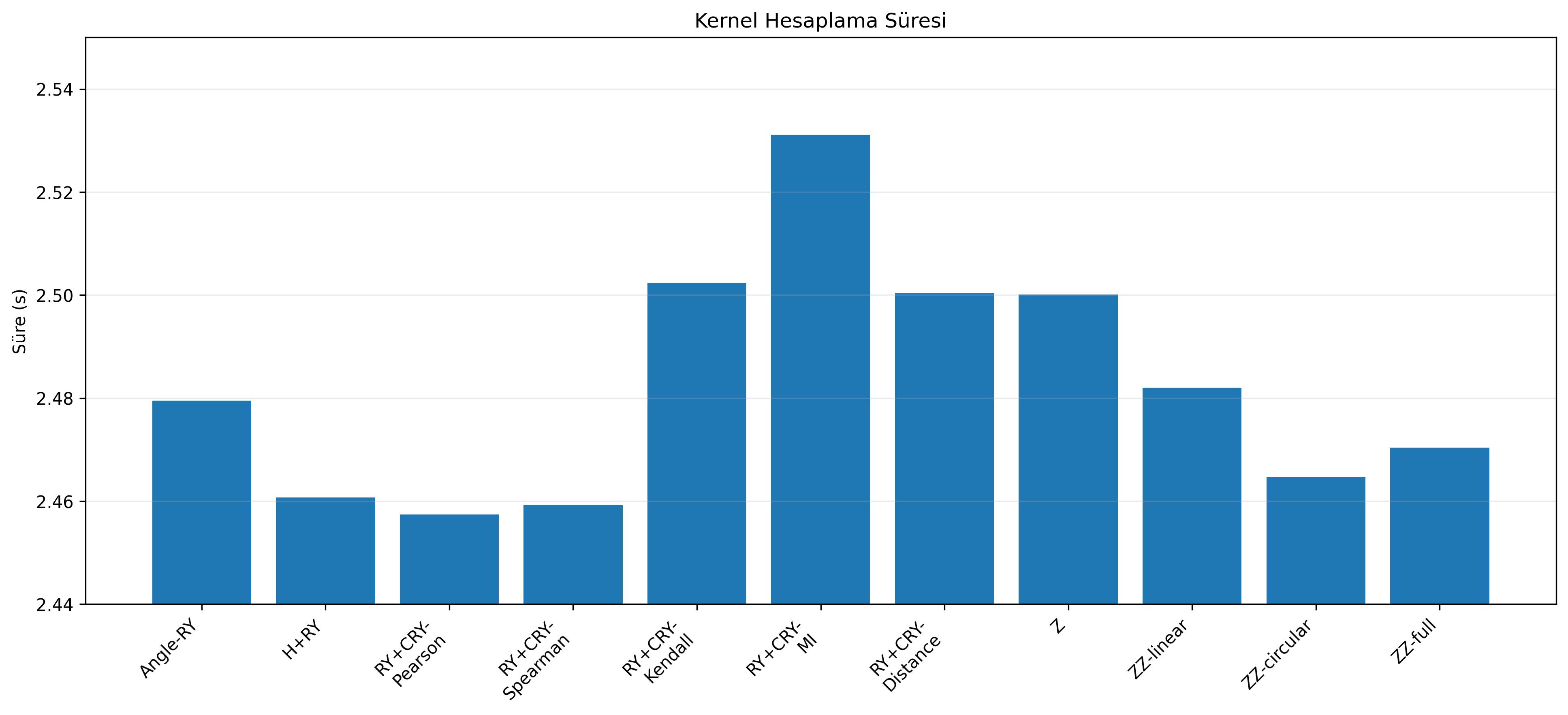
Kernel Time remained within approximately 2.46–2.53 seconds for all methods. Despite substantial differences in circuit complexity, the similar kernel computation times indicate that the primary differences in total computational cost arose from the state vector generation stage.

Training Time ranged from approximately 0.086 to 0.147 seconds across all methods. The lowest training time, approximately 0.086 seconds, was obtained with Z feature Map.
These values are relatively small compared with the state vector computation costs. Therefore, in the Student Performance experiments, the primary source of total computational cost was again the preparation of quantum feature states rather than classical SVM training.
3.4.5 Overall Evaluation of the Student Performance Dataset
The results obtained for the Student Performance Dataset clearly demonstrate that more complex quantum feature maps do not necessarily provide better performance.
Z feature Map achieved the highest test performance among all methods, with a Test Accuracy of 0.944, an F1 score of 0.900, and a ROC-AUC of 0.975. Furthermore, its Accuracy Gap was only 0.024 and its Test Log-Loss was 0.160. At the same time, the circuit required only 26 logical gates and a depth of 2. Therefore, Z feature Map provides the most balanced encoding strategy for this dataset in terms of performance, generalization, and circuit cost.
The RY+CRY methods provided limited but consistent performance improvements over Angle-RY. In particular, the Distance Correlation-based RY+CRY method achieved the highest class-discrimination performance within this group, with a ROC-AUC of 0.963. However, encoding all 78 feature pairs required 325 total gates, 156 CX gates, and a decomposed circuit depth of 82.
Although ZZ linear achieved the second-highest test accuracy of 0.908, it remained behind Z feature Map in terms of Accuracy, F1, ROC-AUC, and generalization gap.
The poorest result was obtained with ZZ full. Despite achieving a training accuracy of 1.000, its test accuracy decreased to 0.712, Recall to 0.020, and F1 to 0.040. Its Accuracy Gap reached 0.288 and its F1 Gap reached 0.960. These results indicate a pronounced overfitting behavior for the fully connected ZZ feature map on the Student Performance Dataset.
Overall, the Student Performance experiments demonstrate that feature-map complexity is not as important as compatibility with the underlying data structure. For this dataset, the low-depth Z feature Map outperformed the more complex RY+CRY and ZZ structures in terms of classification performance, generalization, and computational cost.
3.5 Alzheimer’s Disease Dataset
In the experiments conducted on the Alzheimer’s Disease Dataset, Principal Component Analysis (PCA) was applied to reduce the computational cost associated with the high feature dimensionality in state vector-based calculations. The first 14 principal components (PCs) were retained for quantum feature encoding.
Following PCA, Angle-RY, H+RY, RY+CRY encodings based on different statistical dependency measures, Z feature Map, and ZZ feature Map with different entanglement structures were compared. The evaluation considered classification performance, generalization behavior, quantum circuit complexity, computational cost, and the explained variance retained by PCA.
3.5.1 Dimensionality Reduction with PCA
| Component | Explained Variance | Cumulative Variance |
| PC1 | 0.0403 | 0.0403 |
| PC2 | 0.0387 | 0.0790 |
| PC3 | 0.0379 | 0.1169 |
| PC4 | 0.0370 | 0.1539 |
| PC5 | 0.0364 | 0.1903 |
| PC6 | 0.0363 | 0.2266 |
| PC7 | 0.0355 | 0.2621 |
| PC8 | 0.0350 | 0.2971 |
| PC9 | 0.0341 | 0.3312 |
| PC10 | 0.0337 | 0.3649 |
| PC11 | 0.0334 | 0.3983 |
| PC12 | 0.0331 | 0.4314 |
| PC13 | 0.0327 | 0.4641 |
| PC14 | 0.0320 | 0.4961 |

Table 17 and Fig. 45 show that the first principal component explains approximately 4.03% of the total variance and that no single component dominates the representation. The cumulative explained variance of the first 14 PCs is
| (23) |
The relatively similar explained variance ratios of the components, approximately 3.2–4.0%, indicate that the variance is not concentrated in a small number of dominant components. In other words, the variance structure of the Alzheimer’s Disease Dataset is distributed over a relatively broad feature space.
This observation is important for interpreting the results. Reducing the data to 14 PCs made the quantum simulation computationally feasible, but only approximately half of the variance in the original data was retained. Therefore, the QSVM results reported below reflect not only the effects of the quantum feature encoding strategies but also the amount of information preserved after PCA.
Accordingly, lower test performance obtained with some complex feature maps should not be attributed solely to their quantum circuit structures. Information potentially useful for classification may also have been excluded from the first 14 PCs during dimensionality reduction.
3.5.2 Classification Performance
| Encoding | Train Acc. | Test Acc. | Acc. Gap | Test Prec. | Test Rec. | Test F1 | Test AUC |
| Angle-RY | 0.813 | 0.764 | 0.049 | 0.732 | 0.525 | 0.612 | 0.813 |
| H+RY | 0.813 | 0.764 | 0.049 | 0.732 | 0.525 | 0.612 | 0.813 |
| RY+CRY-Pearson | 0.813 | 0.764 | 0.049 | 0.732 | 0.525 | 0.612 | 0.813 |
| RY+CRY-Spearman | 0.814 | 0.762 | 0.052 | 0.727 | 0.525 | 0.610 | 0.812 |
| RY+CRY-Kendall | 0.813 | 0.762 | 0.051 | 0.727 | 0.525 | 0.610 | 0.812 |
| RY+CRY-MI | 0.871 | 0.760 | 0.111 | 0.752 | 0.480 | 0.586 | 0.803 |
| RY+CRY-Distance | 0.832 | 0.748 | 0.084 | 0.707 | 0.492 | 0.580 | 0.810 |
| Z | 0.965 | 0.706 | 0.259 | 0.683 | 0.316 | 0.432 | 0.768 |
| ZZ linear | 1.000 | 0.646 | 0.354 | 0.000 | 0.000 | 0.000 | 0.593 |
| ZZ circular | 1.000 | 0.646 | 0.354 | 0.000 | 0.000 | 0.000 | 0.579 |
| ZZ full | 1.000 | 0.650 | 0.350 | 1.000 | 0.011 | 0.022 | 0.810 |

Table 18 and Fig. 46 show that the highest test accuracy, 0.764, was obtained with Angle-RY, H+RY, and the Pearson-based RY+CRY encoding.
The Spearman- and Kendall-based RY+CRY methods achieved test accuracies of 0.762, while MI and Distance Correlation achieved 0.760 and 0.748, respectively. Thus, incorporating statistical dependency information through CRY gates did not produce a clear improvement in Accuracy over Angle-RY.
In particular, the identical Accuracy, Precision, Recall, F1, and ROC-AUC values obtained with Pearson-based RY+CRY and Angle-RY indicate that the Pearson-based controlled rotations did not alter the classification decisions within the current PCA-transformed feature space.
In contrast, training accuracy increased substantially as circuit complexity increased. Z feature Map achieved a training accuracy of 0.965, whereas all three ZZ-based methods achieved 1.000. However, their test accuracies decreased to 0.706, 0.646, 0.646, and 0.650, respectively.
These results show that the more complex quantum feature maps represented the training data more strongly, but this increased representational capacity did not translate into improved test performance.

Figure 47 provides a clearer view of the classification behavior, particularly for the ZZ-based feature maps.
For Angle-RY, H+RY, and Pearson-based RY+CRY, Precision, Recall, and F1 were 0.732, 0.525, and 0.612, respectively. Although MI produced a higher Precision of 0.752, its Recall decreased to 0.480, resulting in a lower F1 score of 0.586.
For Z feature Map, Precision was 0.683, whereas Recall was only 0.316 and F1 was 0.432. Thus, despite its high training accuracy, Z feature Map was not able to identify a sufficient proportion of positive-class samples in the test set.
The most pronounced behavior was observed for ZZ linear and ZZ circular. Both methods produced test Precision, Recall, and F1 values of zero, indicating that they failed to correctly identify any positive-class samples in the test set.
Although ZZ full achieved a Precision of 1.000, its Recall was only 0.011 and its F1 score was 0.022. Therefore, high Precision alone does not indicate successful classification. The model produced very few positive predictions and missed nearly all actual positive samples.

The ROC-AUC results provide additional information beyond the threshold-dependent classification metrics. Angle-RY, H+RY, and Pearson-based RY+CRY achieved the highest values at approximately 0.813.
Spearman and Kendall achieved approximately 0.812, while Distance Correlation and MI produced 0.810 and 0.803, respectively. Therefore, changing the statistical dependency measure within the RY+CRY group produced only limited differences in class-separation capability.
Although ZZ full achieved an Accuracy of only 0.650 and an F1 score of only 0.022, its ROC-AUC was 0.810. This result suggests that the model retained some ability to rank samples according to its decision scores, while producing very poor positive-class decisions at the selected classification threshold.
Therefore, ROC-AUC should be interpreted together with F1 and Recall for the Alzheimer’s Disease Dataset.
3.5.3 Generalization Behavior and Log-Loss
| Encoding | Acc. Gap | Prec. Gap | Recall Gap | F1 Gap | AUC Gap | Train Loss | Test Loss |
| Angle-RY | 0.049 | 0.055 | 0.118 | 0.096 | 0.068 | 0.427 | 0.496 |
| H+RY | 0.049 | 0.055 | 0.118 | 0.096 | 0.068 | 0.427 | 0.496 |
| RY+CRY-Pearson | 0.049 | 0.055 | 0.118 | 0.096 | 0.068 | 0.427 | 0.496 |
| RY+CRY-Spearman | 0.052 | 0.063 | 0.120 | 0.100 | 0.070 | 0.425 | 0.496 |
| RY+CRY-Kendall | 0.051 | 0.061 | 0.118 | 0.098 | 0.070 | 0.426 | 0.496 |
| RY+CRY-MI | 0.111 | 0.131 | 0.250 | 0.213 | 0.129 | 0.374 | 0.515 |
| RY+CRY-Distance | 0.084 | 0.111 | 0.182 | 0.159 | 0.083 | 0.412 | 0.499 |
| Z | 0.259 | 0.291 | 0.608 | 0.516 | 0.227 | 0.220 | 0.551 |
| ZZ linear | 0.354 | 1.000 | 1.000 | 1.000 | 0.407 | 0.001 | 0.636 |
| ZZ circular | 0.354 | 1.000 | 1.000 | 1.000 | 0.421 | 0.006 | 0.642 |
| ZZ full | 0.350 | 0.000 | 0.989 | 0.978 | 0.190 | 0.001 | 0.507 |

The lowest Accuracy Gap, 0.049, was obtained with Angle-RY, H+RY, and Pearson-based RY+CRY. Spearman and Kendall also maintained gaps of approximately 0.05.
The gap increased to 0.111 for MI and to 0.259 for Z feature Map. The highest values were obtained with ZZ linear and ZZ circular at 0.354, followed by ZZ full at 0.350.
Thus, as the complexity of the quantum feature map increased, training performance improved while test performance did not improve to the same extent and, in several cases, deteriorated substantially.
In particular, although ZZ linear and ZZ circular classified the training data with an accuracy of 1.000, their test accuracy decreased to 0.646, indicating pronounced overfitting.

The Log-Loss results support the same trend. Angle-RY and Pearson-based RY+CRY produced a Train Log-Loss of approximately 0.427 and a Test Log-Loss of 0.496.
Although Z feature Map reduced the training loss to 0.220, its test loss increased to 0.551. This indicates that the model produced more confident predictions for the training samples, while the quality of its predictions on unseen samples deteriorated.
For ZZ linear and ZZ circular, the training loss approached zero, whereas the Test Log-Loss increased to 0.636 and 0.642, respectively. These were the highest test losses among all methods and further support the evidence of strong overfitting.
The Test Log-Loss of ZZ full was lower than those of the linear and circular variants at 0.507. Nevertheless, since its training loss was only 0.001, the separation between training and test behavior remained substantial.
3.5.4 Quantum Circuit Complexity
| Encoding | H | RY | CRY | CX | Total Gates | Depth | Dec. CX | Dec. Gates | Dec. Depth |
| Angle-RY | 0 | 14 | 0 | 0 | 14 | 1 | 0 | 14 | 1 |
| H+RY | 14 | 14 | 0 | 0 | 28 | 2 | 0 | 28 | 2 |
| RY+CRY-Pearson | 0 | 14 | 91 | 0 | 105 | 26 | 182 | 378 | 89 |
| RY+CRY-Spearman | 0 | 14 | 91 | 0 | 105 | 26 | 182 | 378 | 89 |
| RY+CRY-Kendall | 0 | 14 | 91 | 0 | 105 | 26 | 182 | 378 | 89 |
| RY+CRY-MI | 0 | 14 | 91 | 0 | 105 | 26 | 182 | 378 | 89 |
| RY+CRY-Distance | 0 | 14 | 91 | 0 | 105 | 26 | 182 | 378 | 89 |
| Z | 14 | 0 | 0 | 0 | 28 | 2 | 0 | 28 | 2 |
| ZZ linear | 14 | 0 | 0 | 26 | 67 | 41 | 26 | 67 | 41 |
| ZZ circular | 14 | 0 | 0 | 28 | 70 | 44 | 28 | 70 | 44 |
| ZZ full | 14 | 0 | 0 | 182 | 301 | 77 | 182 | 301 | 77 |


Since 14 PCs were retained after PCA, the Angle-RY circuit contains 14 RY gates. The number of all unique pairwise relationships among the 14 components is
| (24) |
Therefore, each RY+CRY method contains 91 CRY gates.
At the logical level, these circuits contain 105 gates and have a depth of 26. After decomposition, the circuits increase to 378 total gates, 182 CX gates, and a circuit depth of 89.
However, Pearson-based RY+CRY produced exactly the same test performance as Angle-RY. Therefore, within the 14-dimensional PCA representation, encoding all 91 pairwise relationships did not provide an additional test-performance benefit over basic Angle-RY for the Pearson measure.

ZZ linear, ZZ circular, and ZZ full contain 26, 28, and 182 CX gates, respectively. Despite the increase in entanglement density, Test Accuracy, Recall, and F1 did not improve and, particularly for the ZZ variants, decreased substantially.
This result demonstrates that a higher level of entanglement does not necessarily imply better classification performance for the Alzheimer’s Disease Dataset.

In terms of decomposed circuit complexity, the RY+CRY structures are among the most resource-intensive approaches. They require 378 total gates, 182 CX gates, and a circuit depth of 89. By comparison, Angle-RY requires only 14 gates and a depth of 1.
The absence of any test-performance difference between Angle-RY and Pearson-based RY+CRY indicates that encoding all pairwise relationships with controlled rotations is not resource-efficient in the PCA-transformed Alzheimer feature space.
Although ZZ full is substantially more complex, with 301 gates and a depth of 77, its test accuracy decreases from 0.764 for Angle-RY to 0.650. Therefore, no positive relationship between increasing circuit complexity and classification performance was observed for this dataset.
3.5.5 Computational Cost
| Encoding | state vector Time | Kernel Time | Training Time |
| Angle-RY | 5.038 | 4.985 | 0.093 |
| H+RY | 9.268 | 4.871 | 0.094 |
| RY+CRY-Pearson | 53.200 | 4.892 | 0.098 |
| RY+CRY-Spearman | 53.790 | 4.917 | 0.092 |
| RY+CRY-Kendall | 54.285 | 4.965 | 0.091 |
| RY+CRY-MI | 53.897 | 4.969 | 0.125 |
| RY+CRY-Distance | 54.379 | 4.863 | 0.088 |
| Z | 9.380 | 4.905 | 0.130 |
| ZZ linear | 24.458 | 4.915 | 0.151 |
| ZZ circular | 25.650 | 4.906 | 0.160 |
| ZZ full | 119.889 | 5.034 | 0.148 |

The state vector computation times follow the differences in circuit complexity. Angle-RY had the lowest state vector cost at approximately 5.04 seconds. Z feature Map required approximately 9.38 seconds, whereas the RY+CRY methods required approximately 53–54 seconds.
The highest computation time, 119.89 seconds, was obtained with ZZ full.
The state vector cost of ZZ full relative to Angle-RY was approximately
| (25) |
Thus, ZZ full required approximately 23.8 times more state vector computation time, despite producing lower test accuracy and a dramatically lower F1 score.
This observation strongly demonstrates that increased quantum circuit cost did not translate into improved classification performance for the Alzheimer’s Disease Dataset.

Kernel Time remained between approximately 4.86 and 5.03 seconds for all methods. Therefore, the substantial differences in computational cost among the circuit structures originated primarily from state vector generation rather than the kernel computation stage.

Training Time ranged from approximately 0.088 to 0.160 seconds across all methods. These values are very small compared with the state vector computation times.
Therefore, the primary determinant of the total computational cost in the Alzheimer experiments was the preparation of quantum feature states rather than classical SVM optimization.
3.5.6 Overall Evaluation of the Alzheimer’s Disease Dataset
The results obtained for the Alzheimer’s Disease Dataset differ substantially from those observed for the other datasets in this study.
First, the feature space reduced to 14 PCs through PCA retained approximately 49.61% of the total variance. Although this dimensionality reduction was necessary to make the quantum simulation computationally feasible, some information potentially relevant to classification may have been lost. Therefore, the effect of PCA cannot be considered independently of the quantum encoding methods when interpreting the Alzheimer results.
Second, the highest test performance was obtained with the simpler methods. Angle-RY, H+RY, and Pearson-based RY+CRY achieved a Test Accuracy of 0.764, an F1 score of 0.612, and a ROC-AUC of 0.813. Although Pearson-based RY+CRY used a substantially more complex circuit, it provided no test performance advantage over Angle-RY.
Third, training performance increased sharply as circuit complexity increased, while test performance decreased. This behavior was particularly pronounced for the ZZ-based feature maps. All three ZZ methods achieved a training Accuracy of 1.000, whereas their test Accuracy decreased to approximately 0.65.
The Recall and F1 values of ZZ linear and ZZ circular decreased to zero, indicating that these methods were unable to correctly identify the positive class in the test set. Although ZZ full achieved a Precision of 1.000, its Recall was only 0.011 and its F1 score remained at 0.022.
In terms of generalization, the lowest Accuracy Gap, approximately 0.049, was obtained with Angle-RY, H+RY, and Pearson-based RY+CRY, whereas the corresponding values for the ZZ methods increased to approximately 0.35.
A similar pattern is observed in circuit cost. Angle-RY achieved one of the highest test performances with only 14 gates and a circuit depth of 1, whereas ZZ full required 301 logical gates, a circuit depth of 77, and approximately 120 seconds of state vector computation while producing lower test performance.
Overall, the Alzheimer experiments clearly demonstrate that more complex quantum feature maps do not necessarily lead to stronger classification performance. For this dataset, the simple Angle-RY encoding provides a highly competitive solution in terms of performance, generalization, and computational cost.
However, the use of PCA should be explicitly considered when directly comparing the Alzheimer results with those of the other datasets. Since the first 14 PCs explain only approximately half of the total variance, the observed performance limitations may reflect not only the choice of quantum feature map but also the representational feature space produced by dimensionality reduction.
Thus, the Alzheimer’s Disease Dataset demonstrates the importance of jointly considering feature representation, dimensionality reduction, generalization, and circuit complexity when evaluating quantum feature encoding strategies.
3.6 Cross-Dataset Discussion
This study comparatively investigated the effects of different quantum feature encoding strategies on QSVM classification performance, generalization behavior, and quantum circuit complexity across the EEG Eye State Classification, Heart Failure Prediction, Credit Risk, Student Performance, and Alzheimer’s Disease datasets. In addition to relatively simple angle encoding strategies such as Angle-RY and H+RY, RY+CRY structures based on different statistical dependency measures, Z feature Map, and ZZ feature Map variants with different connectivity topologies were evaluated. The results demonstrate that the effect of the quantum feature encoding strategy is neither dataset-independent nor unidirectional; instead, it depends on the interaction among data structure, feature representation, entanglement topology, and model complexity.
When the five datasets are considered together, the first important finding is that more complex quantum feature maps do not consistently provide higher test performance. On the EEG dataset, ZZ full achieved the highest test accuracy of 0.850, but it was also associated with an Accuracy Gap of approximately 0.150 and a high circuit cost. ZZ circular achieved a very similar test accuracy of 0.846 while requiring substantially fewer gates and a much shorter state vector computation time. This observation indicates that maximum test accuracy alone is insufficient to determine the optimal encoding strategy.
A different pattern emerged for the Heart Failure Prediction Dataset. The highest test accuracy, approximately 0.883, was obtained with the Pearson- and Distance Correlation-based RY+CRY structures, whereas Z feature Map achieved a very similar test accuracy of 0.878. In contrast, ZZ linear, ZZ circular, and ZZ full achieved very high training accuracies but decreased in test performance. In particular, ZZ circular achieved a training accuracy of 0.994 but only a test accuracy of 0.757, demonstrating that high circuit complexity did not provide a strong generalization advantage.
For the Credit Risk Dataset, no differences were observed among the quantum feature maps in terms of Test Accuracy, Precision, Recall, or F1; all methods achieved a test accuracy of 0.908. However, ROC-AUC values differed substantially. The Distance Correlation-based RY+CRY method achieved the highest ROC-AUC of 0.663, whereas Z feature Map produced only 0.464. Thus, feature maps that appear equivalent when only Accuracy is considered can behave differently in terms of decision scores and class separability. Accordingly, complementary measures such as ROC-AUC and Log-Loss should be considered together with threshold-dependent metrics when evaluating quantum kernel methods.
For the Student Performance Dataset, Z feature Map produced the strongest and most balanced overall result. It achieved a test accuracy of 0.944, an F1 score of 0.900, and a ROC-AUC of 0.975, while its Accuracy Gap remained only 0.024. In contrast, although ZZ full achieved a training accuracy of 1.000, its test accuracy decreased to 0.712, Recall to 0.020, and F1 to 0.040. This finding clearly demonstrates that a highly expressive quantum feature map can represent the training data very strongly while losing its ability to generalize to unseen data.
The Alzheimer’s Disease Dataset differs methodologically from the other datasets because PCA was applied to manage the high feature dimensionality, and the first 14 PCs were retained. These PCs explained approximately 49.61% of the total variance. Therefore, the Alzheimer results reflect not only the effect of the quantum feature map but also the amount of information retained after dimensionality reduction. Angle-RY, H+RY, and Pearson-based RY+CRY achieved the highest test accuracy of 0.764. In contrast, the Z- and ZZ-based structures substantially increased training performance while test performance decreased. For ZZ linear and ZZ circular, the test F1 score decreased to zero, whereas ZZ full achieved a Precision of 1.000 but only a Recall of 0.011 and an F1 score of 0.022. Therefore, the Alzheimer results should not be attributed solely to the entanglement structure; the amount of classification-relevant information preserved in the PCA-reduced feature space must also be considered.
These differences among the datasets demonstrate that no single quantum feature map is universally superior for all classification problems. ZZ full achieved the highest test accuracy for EEG; Pearson- and Distance Correlation-based RY+CRY were strongest for HEART; Z feature Map was superior for Student Performance; and the simpler Angle-RY and Pearson-based RY+CRY structures performed best for Alzheimer. For Credit Risk, all methods produced the same Accuracy. Thus, the effectiveness of a feature map appears to depend not only on circuit complexity or entanglement density but also on the compatibility between the data distribution and the structure of the resulting quantum feature space.
When the RY+CRY results are considered separately, incorporating statistical relationships between features into controlled rotations was beneficial for some datasets, although the magnitude of the effect was dataset-dependent. For EEG, Pearson-based RY+CRY increased test accuracy from 0.748 with Angle-RY to 0.806, representing a clear improvement. For HEART, the same approach provided a smaller but consistent improvement. For Credit Risk, classification accuracy remained unchanged, but an advantage was observed in ROC-AUC. For Alzheimer, Pearson-based RY+CRY produced exactly the same test performance as Angle-RY. These results indicate that statistical dependency information can be useful for quantum encoding, but its effectiveness depends on the structure of the data.
The cost of RY+CRY circuits must also be considered. For an input dimension , encoding all pairwise relationships requires
| (26) |
controlled connections. For EEG and Alzheimer, 91 CRY connections were used for 14 features or PCs; Student Performance required 78 connections for 13 features; HEART required 55 connections for 11 features; and Credit Risk required 36 connections for 9 features. Thus, an RY+CRY structure in which all pairwise relationships are encoded grows approximately quadratically with the number of input features. In the EEG and Alzheimer experiments, the decomposed RY+CRY circuits reached 182 CX gates and a circuit depth of 89. This indicates that limited performance improvements may sometimes be obtained at the cost of substantial circuit complexity.
An important design implication follows from this observation. It may not be necessary to transfer all pairwise feature relationships into the quantum circuit. Sparse RY+CRY structures in which only the strongest, most stable, or most informative relationships are selected may reduce circuit depth and the number of entangling gates while preserving the performance contribution of dependency information. Such an approach may be particularly important for reducing error accumulation and implementation cost on NISQ devices.
The Z feature Map results also represent an important finding of this study. Z feature Map achieved the strongest overall test performance on the Student Performance Dataset and produced competitive results on both EEG and HEART despite its low circuit complexity. In particular, for Student Performance, it achieved a test accuracy of 0.944 and ROC-AUC of 0.975 using only 26 logical gates and a circuit depth of 2. For EEG, it achieved a test accuracy of 0.834 with 28 logical gates and a depth of 2, while maintaining an Accuracy Gap of 0.060. Therefore, Z feature Map provides a strong balance among performance, generalization, and circuit cost for some datasets.
The ZZ feature Map results clearly demonstrate that the relationship between circuit complexity and classification performance is not linear. Although ZZ full achieved the highest test accuracy for EEG, its improvement over ZZ circular was only 0.004, while the logical gate count increased from 70 to 301. In contrast, denser ZZ connectivity generally increased training accuracy but reduced test performance for HEART, Student Performance, and Alzheimer. Thus, increasing entanglement density does not automatically produce a more effective quantum feature space.
Generalization behavior represents another important common dimension across the five datasets. Particularly for the more complex ZZ-based feature maps, training accuracies frequently approached 1.000 while test performance declined. This behavior was especially pronounced for the Student Performance and Alzheimer’s Disease datasets. When Accuracy Gap, F1 Gap, and Log-Loss are considered together, increasing circuit complexity appears to cause some models to represent the training samples excessively strongly. Therefore, quantum feature encoding strategies should be evaluated not only according to test accuracy but also according to the differences between training and test performance.
A common trend was also observed in computation times. The largest differences among methods occurred during state vector generation, whereas Kernel Time and classical SVM Training Time generally exhibited much smaller variations. For example, ZZ full required approximately 126.6 seconds for EEG and 119.9 seconds for Alzheimer, whereas Angle-RY remained near 5 seconds. In contrast, kernel computation times within the same dataset remained largely stable. This indicates that the primary computational cost in the investigated QSVM framework arises from the generation of quantum feature states rather than classical SVM optimization.
The PCA application to the Alzheimer’s Disease Dataset further emphasizes the relationship between classical preprocessing and quantum feature encoding. The first 14 PCs explained only approximately 49.6% of the total variance, indicating that a substantial amount of variance was excluded during dimensionality reduction. Therefore, particularly for high-dimensional datasets, QML performance should be understood as depending not only on feature-map selection but also on the classical dimensionality reduction strategy. Changing the number of PCA components or employing alternative dimensionality reduction methods may alter the results obtained for the Alzheimer’s Disease Dataset.
3.7 Quantum Feature Encoding Score (QFES)
Evaluating different quantum feature encoding strategies solely in terms of classification performance may overlook differences in generalization ability and computational cost. More complex quantum feature maps may provide high classification performance while also requiring greater circuit depth, larger gate counts, and longer computation times. Therefore, the Quantum Feature Encoding Score (QFES) was defined in this study to jointly evaluate classification performance, generalization behavior, and computational cost.
The performance component of QFES is constructed from Accuracy (), Precision (), Recall (), F1-score (), and ROC-AUC () obtained on the test set. Since all these metrics naturally lie within the interval, they are used directly without additional normalization. The classification performance component is defined as
| (27) |
A higher value therefore indicates stronger overall classification performance for the corresponding quantum feature encoding strategy.
To evaluate generalization behavior, the absolute difference between training and test accuracy is used. The Accuracy Gap () is defined as
| (28) |
A low value indicates that training and test performance are close to each other and that the model exhibits more consistent generalization, whereas a larger indicates greater separation between training and test performance. Since Accuracy Gap naturally lies within , no additional normalization is applied.
Circuit depth (), total gate count (), and state vector computation time () are used to represent quantum circuit complexity and computational cost. Since these variables have different numerical scales, Min–Max normalization is applied before they are incorporated into QFES.
The normalized circuit depth is calculated as
| (29) |
The normalized total gate count is calculated as
| (30) |
Similarly, the normalized state vector computation time is defined as
| (31) |
Thus, , , and are all transformed into the interval. Min–Max normalization is performed separately across the quantum feature encoding strategies compared within each dataset.
To account for the effect of different input dimensions on circuit and computational cost, the generalization and cost terms are scaled by the number of inputs . Here, denotes the number of input features transferred to the quantum feature map. When a direct feature–qubit mapping is used, also corresponds to the number of qubits.
The generalization and computational cost per input are defined as
| (32) |
By combining performance, generalization, and computational cost, QFES is defined as
| (33) |
In Eq. 33, the numerator represents the classification performance of the quantum feature encoding strategy. Increasing Accuracy, Precision, Recall, F1-score, and ROC-AUC therefore increases both the numerator and QFES.
In contrast, increasing Accuracy Gap, normalized circuit depth, gate count, or state vector computation time increases the denominator and consequently reduces QFES.
The constant in the denominator prevents the denominator from approaching zero when the generalization and computational cost terms approach their minimum values. This prevents methods with minimal circuit complexity from obtaining artificially inflated QFES values.
No weighting coefficients are used in the QFES formulation. Accuracy, Precision, Recall, F1-score, and ROC-AUC contribute equally to the classification performance component, whereas Accuracy Gap, circuit depth, gate count, and state vector computation time represent generalization and computational cost. This design avoids introducing subjective predefined weights into the final ranking of the methods.
Consequently, a higher QFES indicates a quantum feature encoding strategy that achieves a more favorable balance among high classification performance, a small training–test accuracy gap, low circuit complexity, and low computation time. QFES is therefore used as a composite evaluation criterion to identify not only the method with the highest predictive performance, but also the method that provides a more balanced performance–generalization–computational cost trade-off.
3.7.1 EEG Eye State Classification Dataset
| Rank | Encoding | Gap | QFES | ||||
| 1 | Z feature Map | 4.1589 | 0.0600 | 0.0132 | 0.0488 | 0.0362 | 4.1124 |
| 2 | ZZ circular | 4.2255 | 0.1493 | 0.5658 | 0.1951 | 0.1850 | 3.9189 |
| 3 | ZZ linear | 4.1993 | 0.1520 | 0.5263 | 0.1847 | 0.1671 | 3.9115 |
| 4 | RY+CRY-Pearson | 4.0224 | 0.0767 | 0.3289 | 0.3171 | 0.4172 | 3.7196 |
| 5 | RY+CRY-Spearman | 3.9891 | 0.0627 | 0.3289 | 0.3171 | 0.4167 | 3.6923 |
| 6 | RY+CRY-Distance | 3.9689 | 0.0800 | 0.3289 | 0.3171 | 0.4229 | 3.6679 |
| 7 | Angle-RY | 3.6212 | 0.0007 | 0.0000 | 0.0000 | 0.0000 | 3.6210 |
| 8 | RY+CRY-Kendall | 3.8937 | 0.0560 | 0.3289 | 0.3171 | 0.4236 | 3.6039 |
| 9 | H+RY | 3.6212 | 0.0007 | 0.0132 | 0.0488 | 0.0394 | 3.5950 |
| 10 | RY+CRY-MI | 3.8539 | 0.0513 | 0.3289 | 0.3171 | 0.4282 | 3.5671 |
| 11 | ZZ full | 4.2441 | 0.1500 | 1.0000 | 1.0000 | 1.0000 | 3.4646 |
For the EEG dataset, Z feature Map achieved the highest QFES value of 4.1124. Although ZZ full had the highest overall classification performance component, , it ranked last in QFES because its normalized circuit depth, gate count, and state vector computation time reached their maximum values. In contrast, Z feature Map combined strong classification performance with low circuit and computational cost, resulting in the highest composite score. ZZ circular and ZZ linear ranked second and third, respectively, because they provided strong predictive performance at substantially lower resource cost than ZZ full.
3.7.2 Heart Failure Prediction Dataset
| Rank | Encoding | Gap | QFES | ||||
| 1 | Angle-RY | 4.4610 | 0.0287 | 0.0000 | 0.0000 | 0.0000 | 4.4493 |
| 2 | Z feature Map | 4.4883 | 0.0156 | 0.0172 | 0.0625 | 0.0688 | 4.4223 |
| 3 | H+RY | 4.4610 | 0.0287 | 0.0172 | 0.0625 | 0.0566 | 4.3950 |
| 4 | RY+CRY-Pearson | 4.5008 | 0.0316 | 0.3276 | 0.3125 | 0.4409 | 4.0874 |
| 5 | RY+CRY-Distance | 4.5028 | 0.0331 | 0.3276 | 0.3125 | 0.4682 | 4.0795 |
| 6 | RY+CRY-Spearman | 4.4872 | 0.0360 | 0.3276 | 0.3125 | 0.4373 | 4.0748 |
| 7 | RY+CRY-Kendall | 4.4842 | 0.0316 | 0.3276 | 0.3125 | 0.4495 | 4.0695 |
| 8 | RY+CRY-MI | 4.4718 | 0.0447 | 0.3276 | 0.3125 | 0.4468 | 4.0547 |
| 9 | ZZ linear | 4.2052 | 0.1869 | 0.5345 | 0.2330 | 0.2218 | 3.7990 |
| 10 | ZZ circular | 4.0394 | 0.2377 | 0.5862 | 0.2500 | 0.2486 | 3.6059 |
| 11 | ZZ full | 4.3696 | 0.1565 | 1.0000 | 1.0000 | 1.0000 | 3.3953 |
For the Heart Failure Prediction Dataset, the highest QFES value, 4.4493, was obtained with Angle-RY. Z feature Map produced a very similar second-best score of 4.4223. Although RY+CRY-Distance and RY+CRY-Pearson produced higher classification performance components than Angle-RY, their greater circuit and state vector costs reduced their overall QFES rankings. In particular, the maximum normalized resource costs of ZZ full reduced its QFES to 3.3953. These results indicate that the simple Angle-RY structure provided the most efficient performance–cost balance for this dataset.
3.7.3 Credit Risk Dataset
| Rank | Encoding | Gap | QFES | ||||
| 1 | Angle-RY | 4.1585 | 0.0013 | 0.0000 | 0.0000 | 0.0000 | 4.1579 |
| 2 | H+RY | 4.1585 | 0.0013 | 0.0217 | 0.0769 | 0.0725 | 4.0803 |
| 3 | Z feature Map | 3.9686 | 0.0067 | 0.0217 | 0.0769 | 0.0949 | 3.8822 |
| 4 | RY+CRY-Distance | 4.1681 | 0.0000 | 0.3261 | 0.3077 | 0.4346 | 3.7259 |
| 5 | RY+CRY-Pearson | 4.1624 | 0.0013 | 0.3261 | 0.3077 | 0.4511 | 3.7142 |
| 6 | RY+CRY-Spearman | 4.1636 | 0.0013 | 0.3261 | 0.3077 | 0.4773 | 3.7056 |
| 7 | RY+CRY-MI | 4.1587 | 0.0013 | 0.3261 | 0.3077 | 0.4921 | 3.6958 |
| 8 | RY+CRY-Kendall | 4.1586 | 0.0013 | 0.3261 | 0.3077 | 0.4981 | 3.6936 |
| 9 | ZZ linear | 4.1236 | 0.0253 | 0.5435 | 0.2821 | 0.3011 | 3.6557 |
| 10 | ZZ circular | 4.1103 | 0.0253 | 0.6087 | 0.3077 | 0.3209 | 3.6047 |
| 11 | ZZ full | 4.1179 | 0.0373 | 1.0000 | 1.0000 | 1.0000 | 3.0788 |
For the Credit Risk Dataset, Angle-RY achieved the highest QFES value of 4.1579. Because Test Accuracy, Precision, Recall, and F1 were largely identical across the methods, resource costs became more influential in the QFES ranking. Although RY+CRY-Distance produced one of the highest performance components, its greater circuit depth, gate count, and state vector cost resulted in fourth place. ZZ full produced the lowest QFES, 3.0788, because it achieved similar test performance at substantially higher resource cost.
3.7.4 Student Performance Dataset
| Rank | Encoding | Gap | QFES | ||||
| 1 | Z feature Map | 4.6238 | 0.0240 | 0.0143 | 0.0526 | 0.0474 | 4.5752 |
| 2 | Angle-RY | 4.1791 | 0.1133 | 0.0000 | 0.0000 | 0.0000 | 4.1430 |
| 3 | H+RY | 4.1791 | 0.1133 | 0.0143 | 0.0526 | 0.0446 | 4.1081 |
| 4 | ZZ linear | 4.3672 | 0.0887 | 0.5286 | 0.1984 | 0.1795 | 4.0567 |
| 5 | RY+CRY-Pearson | 4.2431 | 0.1080 | 0.3286 | 0.3158 | 0.4030 | 3.8968 |
| 6 | RY+CRY-Spearman | 4.2429 | 0.1080 | 0.3286 | 0.3158 | 0.4041 | 3.8963 |
| 7 | RY+CRY-Distance | 4.2441 | 0.1080 | 0.3286 | 0.3158 | 0.4133 | 3.8948 |
| 8 | RY+CRY-Kendall | 4.2421 | 0.1067 | 0.3286 | 0.3158 | 0.4115 | 3.8939 |
| 9 | ZZ circular | 4.2139 | 0.1080 | 0.5714 | 0.2105 | 0.2003 | 3.8879 |
| 10 | RY+CRY-MI | 4.2150 | 0.1107 | 0.3286 | 0.3158 | 0.4177 | 3.8663 |
| 11 | ZZ full | 2.6811 | 0.2880 | 1.0000 | 1.0000 | 1.0000 | 2.1399 |
For the Student Performance Dataset, Z feature Map clearly achieved the highest QFES value, 4.5752. It also produced the highest total performance component, , while maintaining a low Accuracy Gap and very low normalized circuit costs. Angle-RY ranked second because of its minimum circuit cost despite its lower performance component. ZZ full produced a substantially lower QFES of 2.1399 because of its poor test Recall and F1, large Accuracy Gap, and maximum resource costs.
3.7.5 Alzheimer’s Disease Dataset
| Rank | Encoding | Gap | QFES | ||||
| 1 | Angle-RY | 3.4464 | 0.0487 | 0.0000 | 0.0000 | 0.0000 | 3.4345 |
| 2 | H+RY | 3.4464 | 0.0487 | 0.0132 | 0.0488 | 0.0368 | 3.4105 |
| 3 | RY+CRY-Pearson | 3.4464 | 0.0487 | 0.3289 | 0.3171 | 0.4193 | 3.1924 |
| 4 | RY+CRY-Spearman | 3.4360 | 0.0520 | 0.3289 | 0.3171 | 0.4245 | 3.1809 |
| 5 | RY+CRY-Kendall | 3.4362 | 0.0507 | 0.3289 | 0.3171 | 0.4288 | 3.1805 |
| 6 | RY+CRY-MI | 3.3820 | 0.1107 | 0.3289 | 0.3171 | 0.4254 | 3.1186 |
| 7 | RY+CRY-Distance | 3.3373 | 0.0840 | 0.3289 | 0.3171 | 0.4296 | 3.0820 |
| 8 | Z feature Map | 2.9053 | 0.2587 | 0.0132 | 0.0488 | 0.0378 | 2.8327 |
| 9 | ZZ full | 2.4938 | 0.3500 | 1.0000 | 1.0000 | 1.0000 | 2.0123 |
| 10 | ZZ linear | 1.2391 | 0.3540 | 0.5263 | 0.1847 | 0.1691 | 1.1387 |
| 11 | ZZ circular | 1.2246 | 0.3540 | 0.5658 | 0.1951 | 0.1795 | 1.1210 |
For the Alzheimer’s Disease Dataset, Angle-RY achieved the highest QFES value of 3.4345. Although H+RY and Pearson-based RY+CRY produced the same overall classification performance component, their additional circuit complexity and computation time caused them to rank below Angle-RY. Z feature Map exhibited a lower QFES because its higher training performance was accompanied by a large Accuracy Gap. The ZZ methods ranked near the bottom because of both low test Recall and F1 values and higher resource costs. Since the dataset was represented using 14 PCs after PCA, these results should also be interpreted in the context of the information retained in the reduced feature space.
When the QFES results across all five datasets are considered together, no single quantum feature encoding method is optimal for every dataset. Z feature Map achieved the highest QFES for the EEG Eye State Classification and Student Performance datasets, whereas Angle-RY ranked first for the Heart Failure Prediction, Credit Risk, and Alzheimer’s Disease datasets.
This finding demonstrates that the method with the highest raw classification performance does not necessarily produce the highest QFES. In particular, methods with high circuit complexity, such as ZZ full, can produce strong Accuracy or ROC-AUC values on some datasets but receive lower QFES rankings because of increased Accuracy Gap, circuit depth, gate count, and state vector computation time.
In contrast, simpler structures such as Angle-RY and Z feature Map frequently provided sufficient classification performance at substantially lower computational cost, resulting in a more favorable performance–generalization–resource cost balance.
4 Conclusion
This study systematically evaluated different quantum feature encoding strategies for QSVM-based binary classification across multiple datasets. The results demonstrate that the choice of quantum feature encoding affects not only classification performance but also model generalization, quantum circuit complexity, and computational cost.
When the results obtained from the different datasets are considered together, no single quantum feature map was found to be universally superior across all classification problems. While more complex and highly entangled feature maps achieved higher test performance for some datasets, simpler encoding strategies provided better generalization and a more favorable balance between predictive performance and circuit cost for others. These findings indicate that the effectiveness of a quantum feature map depends not only on its circuit structure but also on the statistical characteristics of the dataset and the structure of the corresponding feature space.
Incorporating statistical dependencies between features into quantum encoding through RY and CRY gates improved classification performance over basic angle encoding for some datasets. However, encoding all pairwise feature relationships through controlled rotations substantially increased circuit depth and the number of entangling gates. Therefore, the benefit of transferring statistical dependency information into quantum circuits should be evaluated by considering the resulting improvement in classification performance together with the additional circuit cost.
Similarly, the results obtained with ZZ feature Map demonstrate that increasing entanglement density does not necessarily produce a more effective quantum feature space. In several experiments, denser connectivity structures substantially increased training performance without providing a comparable improvement in test performance, resulting in larger training–test gaps. This observation suggests that the expressive capacity of a quantum feature map should be considered together with its ability to generalize to unseen data.
To provide a unified assessment of classification performance, generalization, and quantum computational cost, the Quantum Feature Encoding Score (QFES) was also employed in this study. The QFES results showed that the encoding strategy with the highest raw classification performance was not necessarily the most favorable overall approach. Methods that achieved competitive test performance with lower circuit depth, fewer gates, and shorter state vector computation times could provide a better balance among predictive performance, generalization, and resource requirements.
Overall, the selection of a feature encoding strategy for QSVM and quantum-kernel-based classification should not be based solely on individual performance measures such as Accuracy or ROC-AUC. Classification performance, training–test differences, circuit depth, gate count, and computational time should instead be considered jointly. The findings of this study suggest that data-aware and resource-conscious approaches to quantum feature encoding may provide a more appropriate framework for designing efficient quantum machine learning models.
Future studies may investigate sparse RY+CRY structures in which only the strongest or most informative statistical relationships are encoded, rather than introducing controlled rotations between all feature pairs. Such an approach may preserve the benefits of dependency-aware encoding while reducing circuit depth and entangling-gate requirements. Furthermore, experiments involving different input dimensions, alternative dimensionality reduction techniques, and real NISQ hardware may provide further insight into the scalability, robustness, and practical applicability of quantum feature encoding strategies.
References
- [1] (1980) The computer as a physical system: a microscopic quantum mechanical hamiltonian model of computers as represented by turing machines. Journal of Statistical Physics 22 (5), pp. 563–591. External Links: Document Cited by: §1.
- [2] (1985) Quantum theory, the church–turing principle and the universal quantum computer. Proceedings of the Royal Society of London. Series A, Mathematical and Physical Sciences 400 (1818), pp. 97–117. External Links: Document Cited by: §1.
- [3] (1997) On the power of quantum computation. SIAM Journal on Computing 26 (5), pp. 1474–1483. External Links: Document Cited by: §1.
- [4] (1997) Polynomial-time algorithms for prime factorization and discrete logarithms on a quantum computer. SIAM Journal on Computing 26 (5), pp. 1484–1509. External Links: Document Cited by: §1.
- [5] (1997) Quantum mechanics helps in searching for a needle in a haystack. Physical Review Letters 79 (2), pp. 325–328. External Links: Document Cited by: §1.
- [6] (2015) An introduction to quantum machine learning. Contemporary Physics 56 (2), pp. 172–185. External Links: Document Cited by: §1.
- [7] (2017) Quantum machine learning. Nature 549 (7671), pp. 195–202. External Links: Document Cited by: §1.
- [8] (2019) Quantum machine learning. National Science Review 6 (1), pp. 26–28. External Links: Document Cited by: §1.
- [9] (2023) Quantum machine learning: a review and case studies. Entropy 25 (2), pp. 287. External Links: Document Cited by: §1.
- [10] (2024) Systematic literature review: quantum machine learning and its applications. Computer Science Review 51, pp. 100619. External Links: Document Cited by: §1.
- [11] (2024) Quantum machine learning: classifications, challenges, and solutions. Journal of Industrial Information Integration 42, pp. 100736. External Links: Document Cited by: §1.
- [12] (2025) Quantum machine learning: a comprehensive review of integrating ai with quantum computing for computational advancements. MethodsX 14, pp. 103318. External Links: Document, ISSN 2215-0161 Cited by: §1.
- [13] (2026) A survey of quantum machine learning: foundations, algorithms, frameworks, data and applications. ACM Computing Surveys 58 (4), pp. 91. External Links: Document Cited by: §1.
- [14] (2026) Quantum machine learning: a comprehensive survey of models, challenges, and future directions. Theoretical Computer Science 1074, pp. 115923. External Links: Document Cited by: §1.
- [15] (2024) Quantum data encoding: a comparative analysis of classical-to-quantum mapping techniques and their impact on machine learning accuracy. EPJ Quantum Technology 11, pp. 72. External Links: Document Cited by: §1.
- [16] (2021) Universal approximation property of quantum machine learning models in quantum-enhanced feature spaces. Physical Review Letters 127, pp. 090506. External Links: Document Cited by: §1.
- [17] (2023) Quantum feature maps for graph machine learning on a neutral atom quantum processor. Physical Review A 107, pp. 042615. External Links: Document Cited by: §1.
- [18] (2024) Quantum visual feature encoding revisited. Quantum Machine Intelligence 6, pp. 61. External Links: Document Cited by: §1.
- [19] (2025) Effective quantum feature maps in quantum extreme reservoir computation from the xy model. Physical Review A 111, pp. 022431. External Links: Document Cited by: §1.
- [20] (2026) Comparative performance analysis of quantum feature maps for quantum kernel-based machine learning. Scientific Reports 16, pp. 8142. External Links: Document Cited by: §1.
- [21] (2026) Quantum feature-map learning with reduced resource overhead. Physical Review Research 8, pp. 023247. External Links: Document Cited by: §1.
- [22] (2026) A correlation aware quantum feature map for variational quantum classification. External Links: 2606.21570 Cited by: §1.
- [23] (2014) Quantum support vector machine for big data classification. Physical Review Letters 113 (13), pp. 130503. External Links: Document Cited by: §1.
- [24] (2024) The complexity of quantum support vector machines. Quantum 8, pp. 1225. External Links: Document Cited by: §1.
- [25] (2024) Quantum support vector machines for classification and regression on a trapped-ion quantum computer. Quantum Machine Intelligence 6, pp. 31. External Links: Document Cited by: §1.
- [26] (2023) Universal expressiveness of variational quantum classifiers and quantum kernels for support vector machines. Nature Communications 14, pp. 576. External Links: Document Cited by: §1.
- [27] (2023) Quantum support vector machine without iteration. Information Sciences 635, pp. 25–41. External Links: Document Cited by: §1.
- [28] (2022) Pairwise classification using quantum support vector machine with kronecker kernel. Quantum Machine Intelligence 4, pp. 22. External Links: Document Cited by: §1.
- [29] (2026) Quantum support vector machines and quantum kernel methods. Software: Practice and Experience. External Links: Document Cited by: §1.
- [30] (2023) Application of quantum machine learning using quantum kernel algorithms on multiclass neuron m-type classification. Scientific Reports 13, pp. 11541. External Links: Document Cited by: §1.
- [31] (2024) An enhanced approach for predicting air pollution using quantum support vector machine. Scientific Reports 14, pp. 19521. External Links: Document Cited by: §1.
- [32] (2024) Implementation and performance evaluation of quantum machine learning algorithms for binary classification. Software 3 (4), pp. 498–513. External Links: Document Cited by: §1.
- [33] (2025) Benchmarking quantum machine learning kernel training for classification tasks. IEEE Transactions on Quantum Engineering, pp. 1–15. External Links: Document Cited by: §1.
- [34] (2025) Investigating quantum feature maps in quantum support vector machines for lung cancer classification. Journal of Artificial Intelligence Research and Innovation 1 (1), pp. 100–110. External Links: Document Cited by: §1.
- [35] (2025) Enhancing quantum support vector machine for healthcare applications using custom feature maps. Knowledge-Based Systems 320, pp. 113669. External Links: Document Cited by: §1.
- [36] (2025) Quantum kernel methods under scrutiny: a benchmarking study. Quantum Machine Intelligence 7, pp. 58. External Links: Document Cited by: §1.
- [37] (2015) Time domain measures of inter-channel eeg correlations: a comparison of linear, nonparametric and nonlinear measures. Cognitive Neurodynamics 9, pp. 1–15. Cited by: §1.
- [38] (1994) Using mutual information for selecting features in supervised neural net learning. IEEE Transactions on Neural Networks 5 (4), pp. 537–550. External Links: Document Cited by: §1.
- [39] (2012) Feature screening via distance correlation learning. Journal of the American Statistical Association 107 (499), pp. 1129–1139. Cited by: §1.
- [40] (2022) Feature selection based on distance correlation: a filter algorithm. Journal of Applied Statistics 49 (2), pp. 411–426. External Links: Document Cited by: §1.
- [41] (2023) Distance correlation-based feature selection in random forest. Entropy 25 (9), pp. 1250. External Links: Document Cited by: §1.
- [42] (2024) Feature selection with distance correlation. Physical Review D 109, pp. 054009. External Links: Document Cited by: §1.
- [43] (2022) Eye state classification eeg dataset. Kaggle. Note: Kaggle DatasetAccessed: 2026-08-21 External Links: Link Cited by: §2.8.
- [44] (2021) Heart failure prediction dataset. Kaggle. Note: Kaggle DatasetAccessed: 2026-08-21 External Links: Link Cited by: §2.8.
- [45] Credit risk dataset. Kaggle. Note: Kaggle DatasetAccessed: 2026-08-21 External Links: Link Cited by: §2.8.
- [46] Student performance dataset. Kaggle. Note: Kaggle DatasetAccessed: 2026-08-21 External Links: Link Cited by: §2.8.
- [47] (2024) Alzheimer’s disease dataset. Kaggle. External Links: Document, Link Cited by: §2.8.