Long-time Dynamics of Many-body Open Quantum Systems using Quantum Generating Functions
Abstract
The interplay between coherent unitary evolution and environment-induced dissipation can give rise to a wide range of non-equilibrium dynamics in open quantum systems, ranging from interesting transport phenomena to dynamical phase transitions. However, accessing such long-time dynamics remains challenging for the existing methods developed for the simulation of many-body open quantum systems. We address this problem by developing a quantum generating function (QGF) formalism for open many-body systems for both ensemble-averaged dynamics governed by a Markovian quantum master equation and trajectory-resolved dynamics described by the quantum trajectory formalism, including quantum jumps, and quantum state diffusion. Our approach computes the dynamics of higher-order moments and fluctuation statistics without explicitly evolving the quantum state, thereby providing an efficient and scalable approach for investigating many-body open quantum systems. We demonstrate the versatility of the formalism by applying it to both the integrable open XXZ chain and the nonintegrable open next-nearest-neighbor XXZ spin chain, where it uncovers distinct initial state dependent long-time transport regimes. Our work establishes quantum generating functions as an efficient and scalable framework for investigating long-time dynamics in open quantum many-body systems.
Introduction.– Understanding the dynamics of many-body open quantum systems is a central challenge in modern condensed matter physics, both from theoretical [32, 49, 11, 25, 38, 69, 43, 47, 60, 52] and experimental perspectives [6, 7, 29, 42, 35, 71, 76, 34]. These systems offer a rich playground of nonequilibrium phenomena with interesting long time dynamics and steady state properties which are the result of the interplay between coherent unitary dynamics and environment induced dissipation [51, 20, 22, 16]. This can result in a variety of transport regimes, e.g. ballistic, diffusive, subdiffusive, superdiffusive, and insulating [38, 50, 57, 56], different thermodynamics functioning regimes [5, 55], and dynamical transitions [36, 18]. However, understanding the long time behaviour of large open many-body systems has remained a central challenge due to the exponential growth of Hilbert space dimension. Over the years, several numerical techniques have been developed which have their own advantages and limitations, for example, tensor network based matrix product states (MPS) are useful to represent low entangled state, whereas numerics become expensive with increasing entanglement [59, 12]. On the other hand, neural network states can efficiently represent states with volume-law entanglement, but limited to short times or steady states [39, 61, 64, 28, 68, 27, 65, 73, 41, 53, 66, 75].
A recent breakthrough in the simulation of long-time dynamics in isolated quantum many-body systems has been achieved through the introduction of the quantum generating function (QGF) formalism [63], which is based on full counting statistics of an observable and introduces a counting operator whose operator-space entanglement can remain comparatively low even at long times. The idea of evolving the counting operator instead of states facilitates the computation of different moments of an observable over significantly long timescales. This approach has recently been applied to isolated many-body systems to compute the statistics of integrated charge currents where various interesting long time dynamics is observed [44, 46]. However, an efficient generalization of the QGF formalism to open quantum many-body systems is still an open problem. Establishing such a framework would potentially provide access to a wide range of long-time dynamical phenomena, including transport, dynamical phase transitions, and other emergent nonequilibrium behaviors that have remained largely inaccessible to existing numerical approaches. Furthermore, studies of long-time quantum dynamics and transport in many-body systems have largely focused on initial states close to infinite temperature or highly polarized states, such as domain-wall configurations. In contrast, our work investigates dynamical transport in a fundamentally different manner, which broadens significantly the types of initial conditions that can be considered.
In this work, we show how one can study the long-time dynamics of many-body open quantum systems in regimes where the conventional state-evolution methods by various numerical techniques become computationally impractical. This relies on extending the methods based on QGF to open quantum systems. Importantly, Markovian open quantum dynamics in the Gorini-Kossakowski-Sudarshan-Lindblad (GKSL) form, [26, 40], is commonly described within two complementary frameworks [8, 10, 54, 15]: (i) Ensemble-averaged description governed by the GKSL quantum master equation (QME) [40, 26], and (ii) trajectory-resolved description provided by quantum trajectory formalism, whether with quantum jump or with a state diffusion equation [48, 24, 9, 10, 13]. Each approach can allow to better study different quantum systems, depending on the specific features of the setup. Here, we show how to formulate the QGF approach within both frameworks.
QGF Procedure for open systems.– The time evolution of the system is governed by the Liouvillian superoperator according to , where comprises both the unitary contribution generated by the Hamiltonian and the dissipative contribution arising from environmental interactions. Within the QGF framework, one can compute either the moments of the observable itself (single time measurement protocol) or that of the net transferred quantity (two time measurement protocol). To compute the QGF for , we employ the two-time measurement protocol–measuring the state at initial time and at time . Therefore, starting from the the initial state , a projective measurement of the observable is performed which leads to the post measurement state , where is an eigenvalue of the operator . The state is then evolved by the effect of Liouvillian followed by a second projective measurement at time which gives the final post-measurement state . Hence, the probability distribution of the net transferred charge during the time interval is given by [2],
| (1) |
The QGF is obtained by performing a Fourier transformation of with respect to the counting field . It is given as
| (2) |
where , which we refer to as the counting operator. To obtain Eq. (2), we have replaced the Dirac delta function by and used the relation where is the adjoint Liouvillian. Interestingly, for , for all times which is a trivial matrix product operator (MPO). This follows from the fact that the identity operator is the right eigenvector of with eigenvalue , a property referred to as the unitality of . Consequently, for small values of , the counting operator can remain close to the identity operator up to a significantly large time window. As a result, the bond dimension of remains low throughout the dynamics and can always be controlled by appropriately tuning . However, choosing to be too small is also not optimal, as it requires a larger bond dimension to accurately capture the dynamics [1]. This controllability of the bond dimension makes the simulation of particularly advantageous for simulating long-time open many-body dynamics, especially in comparison with conventional state evolution using MPS, where the bond dimension can, in principle, grow uncontrollably with time.
In this work, we use the Time Evolution Block Decimation (TEBD) algorithm to simulate the time dynamics of and use that to compute the QGF at each time instant. From the QGF, we analytically continue to the complex plane and expand in orders of as [63],
| (3) |
This complex plane extension helps to obtain different moments appropriately by choosing proper real and imaginary part of for a given value. For example, the first and second moment of are given by
| (4) | ||||
| (5) |


where we choose . To obtain the higher moments , one may need to choose much smaller value of and an appropriate phase [63]. Following this recipe, one can analyze the long time dynamics of different moments in open many body systems.
Long time dynamics of many-body quantum systems with a localized particle injection.– We now apply the developed QGF framework to an open many-body spin- lattice system governed by the QME
| (6) |
Here, the Hamiltonian is given by
| (7) |
For , Eq. (7) reduces to the integrable XXZ model, whereas corresponds to the non-integrable next-nearest-neighbour XXZ (nnn-XXZ) model. The dissipative dynamics is encoded in the jump operators , appearing in the second and third terms of Eq. (6). For these models, we focus on the quantum dynamics of the moments of transferred magnetization operator where , when the lattice is subjected to a single dissipative channel with jump operator , corresponding to a local injection of spin excitations at the left boundary of the chain, thereby driving it out of equilibrium. Here is the injection rate and is the spin-excitation operator acting on the first lattice site. We consider three different initial states for both XXZ and nnn-XXZ models: (a) the Néel state, ; (b) an Ising-type state [33], , where if and otherwise; and (c) a fully polarized state with all spins down, . We investigate quantum dynamics for the first and second moment and observe interesting initial condition dependent long-time dynamics. Open quantum dynamics study for such a setup over a large time-window is significantly limited. For example, performing the conventional state evolution via MPS under such a scenario can result in an uncontrolled growth of the bond dimension. The developed QGF method, instead, can provide access to long time dynamics and hence can potentially showcase different interesting dynamical transport regimes. The different transport regimes can be distinguished by the dynamical scaling of the moments of the transferred charge with time. In particular, ballistic transport is characterized by , whereas diffusive transport exhibits the scaling . Superdiffusive and subdiffusive transport are characterized by , with and , respectively.
In Fig. 1, we present the results of the long time dynamics for the three different initial states discussed previously. The open quantum dynamics is simulated using the TEBD algorithm by evolving the initial counting operator under the action of adjoint Liouvillian which is given by,
| (8) |
Here we employ a second-order Suzuki-Trotter decomposition of with a time step , and set and . In Fig. 1(a)-(c), we plot the first and second moments, and , for the XXZ chain with anisotropy parameter starting from the Néel state [Fig. 1(a)], the Ising-type state [Fig. 1(b)], and the fully polarized down state [Fig. 1(c)]. We find a striking dependence of the long-time transport dynamics on the initial state. For the Néel state, both and exhibit an initial growth proportional to at very early times , followed by a ballistic transport regime characterized by and . In contrast, for the Ising-type initial state, the initial growth crosses over to a superdiffusive regime at late times, with and . For the fully polarized down state, the early-time behavior is qualitatively different: both moments initially grow linearly in time rather than . This is followed by a transient superdiffusive regime, with and , before crossing over to diffusive behavior at late times, characterized by and . These results demonstrate that the nonequilibrium transport dynamics of the open XXZ chain can depend sensitively on the initial state, giving rise to a plethora of transient and asymptotic transport regimes. These intriguing dynamical regimes warrant a more thorough theoretical investigation. In contrast, the results for the nnn-XXZ chain presented in Fig. 1(d)-(f) are qualitatively similar for all three initial states, i.e., and . This insensitivity to the choice of initial state can be attributed to the chaotic nature of the underlying Hamiltonian. To highlight the limitations of conventional state evolution, we further plot obtained from direct state evolution (scattered plots in Fig. 1), where the density matrix is evolved under the GKSL equation. We find that state evolution rapidly becomes inaccurate at long times for both the Néel and Ising-type initial states, whereas it remains reliable for the fully polarized down state. The QGF therefore provides access to long-time transport dynamics revealing initial state dependent rich transport phenomena that are otherwise inaccessible through conventional state evolution. We further investigate the dependence of on at different times and extract the probability distribution of the injected charge via inverse Fourier transform [1].
In the Supplemental Material, we further apply the developed QGF framework to a different open many-body setup, where the XXZ and nnn-XXZ chains are subjected to weak local dephasing at every lattice site. Owing to the weak dephasing, the conventional state-evolution approach once again becomes computationally intractable at long times, making the QGF framework necessary for investigating the long-time dynamics.
QGF approach for quantum trajectories.– An alternative and widely employed approach to study open quantum systems is the quantum trajectories formalism. In this approach, instead of evolving the mixed quantum state , one evolves pure-state trajectories in a stochastic manner by unraveling the QME. As we will show later, this approach naturally gives insight into the statistics of the measurements. Furthermore, this approach offers a significant numerical advantage because a pure state is represented by a -dimensional vector in Hilbert space, whereas a vectorized mixed state is represented by a -dimensional vector in Liouville space. To accurately recover the open-system dynamics, however, averaging over sufficiently large ensemble of stochastic trajectories is required. Since individual trajectories are statistically independent, the required ensemble averaging can be performed efficiently using parallel computation. Beyond this computational advantage, individual quantum trajectories have been experimentally accessed, for example through continuous monitoring [72, 30, 31] across a variety of quantum platforms [58, 67, 45]. It has thus enabled the observation and investigation of a variety of emergent phenomena, such as measurement-induced phase transitions [62, 19, 4], measurement-induced symmetry restoration [14, 21], and charge-sharpening transitions [3, 17].
Motivated by these developments, we extend the QGF approach to individual quantum trajectories to avoid evolving the pure quantum states explicitly. We can write the evolution of a stochastic trajectory as , where we refer as the generator of the evolution for the quantum trajectory from time to . Note that in general, the generator can depend on the instantaneous state . For a single quantum trajectory, we then define a trajectory-resolved quantum generating function (QGF) as,
| (9) |
where, represents the evolution operator evolving a single trajectory. Consequently, the counting operator evolves as . For notational simplicity, we suppress the explicit dependence on hereafter and write instead of . Similar to the ensemble-averaged evolution governed by the GKSL master equation, the trajectory propagator also satisfies the unitality property i.e., at every time step. Therefore, for sufficiently small , remains close to the identity operator, making its propagation computationally efficient.


In what follows, we discuss two different kinds of stochastic trajectory protocols, namely the quantum jump (QJ), and the quantum state diffusion (QSD) for the XXZ setup with locally injected spin excitation, as discussed before. For the (QJ) protocol [13, 37] the quantum state evolves via stochastic Schrödinger equation (SSE) given by,
| (10) |
where . is a Poisson stochastic variable that takes value with probability and with probability . For this protocol, we compute the total injected charge along each quantum-jump trajectory using the QGF in Eq. (9) starting from the Néel state for XXZ chain with . It is obtained as,
| (11) |
where we choose to be real by setting . Here, we are interested in the distribution of the injected charge by sampling a large number of quantum trajectories. Interestingly, for the QJ protocol, if one samples a sufficiently large number of quantum trajectories and computes the total injected charge for each trajectory, and finally constructs its distribution (here ), the resulting distribution is exactly identical to obtained from the Fourier transform of the ensemble-averaged generating function under the GKSL master equation [37] [1]. We sample an ensemble of quantum trajectories to obtain the probability distribution , shown in Fig. 2(a) at different time snapshots. Owing to the discrete nature of quantum jumps generated by , the injected charge is always quantized in integer units, increasing by one with each jump event. The inset of Fig. 2(a) shows the time evolution of the injected charge for trajectories. The staircase-like evolution, consisting of unit-height jumps separated by plateaus, clearly distinguishes the jump events from the no-jump evolution which is governed by .
For the same setup, we next implement the quantum state diffusion (QSD) protocol [23] which is another type of quantum trajectory and corresponds to a different continuous and weak measurement scheme. The experimental realization of such a process is possible through homodyne detection experiments [74, 70, 37]. The evolution of the pure state under the QSD is given by,
| (12) |
Here, is Gaussian noise with mean and variance describing a Wiener process. Once again, we sample quantum trajectories and obtain the injected charge for each trajectories using QGF in Eq. (10). We plot the distribution of injected charge in the diffusive trajectories for different time snapshots in Fig. 2(b), and the evolution of different trajectories in its inset. The distribution is Gaussian due to the underlying Wiener process. Moreover, unlike the QJ scenario, here the injected charge can take non-integer values as well, which makes this distribution significantly different from . Overall, the average injected charge remains identical for both the QJ and QSD protocols.
Summary.– In this work, we have developed a QGF formalism for Markovian open quantum systems. We have formulated the QGF framework for both the ensemble-averaged GKSL quantum master equation and stochastic quantum trajectories, each giving different insights into the dynamics, and each having different computational advantages. This generalization is fundamentally enabled by the unitality of the adjoint Liouvillian superoperator for the GKSL dynamics and of the trajectory propagator for quantum trajectories, both of which admit the identity operator as an eigenoperator.
We have demonstrated the versatility of the proposed framework in open quantum many-body systems, where conventional state-evolution methods become computationally extensive due to the rapid growth of operator-space or trajectory entanglement. In particular, we have studied the integrable XXZ and next-nearest-neighbor XXZ chains subjected to boundary spin injection and shown that the QGF formalism efficiently computes the higher-order moments of magnetization transport at long times. This allowed us to uncover a intriguing initial state dependence on the long-time transport regimes for the XXZ model. Furthermore, we have generalized the framework to both quantum-jump and quantum-state-diffusion unravelings by introducing a trajectory-resolved QGF, in this way allowing the simulate different types of measurement scenarios.
Overall, this work establishes the QGF formalism as a computationally efficient framework for probing long time dynamics in many-body open quantum systems, particularly in regimes where conventional state-based approaches become intractable. Promising future directions include extending the framework to non-Markovian open-system dynamics and strong system-environment coupling regimes.
Acknowledgements.– BKA acknowledges the CRG grant No. CRG/2023/003377 from ANRF, Government of India. KG would like to acknowledge the Prime Minister’s Research Fellowship (ID- 0703043), Government of India for funding. KG and BKA acknowledge the National Supercomputing Mission (NSM) for providing computing resources of ‘PARAM Brahma’ at IISER Pune, which is implemented by C-DAC and supported by the Ministry of Electronics and Information Technology (MeitY) and DST, Government of India. DP acknowledges support from the Singapore Ministry of Education from grant MOE-T2EP50123-0017.
References
- [1] (-) . See Supplementary Material , pp. . External Links: Document Cited by: Long-time Dynamics of Many-body Open Quantum Systems using Quantum Generating Functions, Long-time Dynamics of Many-body Open Quantum Systems using Quantum Generating Functions, Long-time Dynamics of Many-body Open Quantum Systems using Quantum Generating Functions.
- [2] (2012) Full-counting statistics of heat transport in harmonic junctions: transient, steady states, and fluctuation theorems. Phys. Rev. E 85, pp. 051142. External Links: Document, Link Cited by: Long-time Dynamics of Many-body Open Quantum Systems using Quantum Generating Functions.
- [3] (2022) Entanglement and charge-sharpening transitions in u(1) symmetric monitored quantum circuits. Phys. Rev. X 12, pp. 041002. External Links: Document, Link Cited by: Long-time Dynamics of Many-body Open Quantum Systems using Quantum Generating Functions.
- [4] (2021) Entanglement transition in a monitored free-fermion chain: from extended criticality to area law. Phys. Rev. Lett. 126, pp. 170602. External Links: Link Cited by: Long-time Dynamics of Many-body Open Quantum Systems using Quantum Generating Functions.
- [5] F. Binder, L. A. Correa, C. Gogolin, J. Anders, and G. Adesso (Eds.) (2018) Thermodynamics in the quantum regime: fundamental aspects and new directions. Fundamental Theories of Physics, Vol. 195, Springer International Publishing. External Links: Document, ISBN 978-3-319-99045-3 Cited by: Long-time Dynamics of Many-body Open Quantum Systems using Quantum Generating Functions.
- [6] (2012) Quantum simulations with trapped ions. Nature Physics 8 (4), pp. 277–284. External Links: Link Cited by: Long-time Dynamics of Many-body Open Quantum Systems using Quantum Generating Functions.
- [7] (2012) Quantum simulations with ultracold quantum gases. Nature Physics 8 (4), pp. 267–276. External Links: Link Cited by: Long-time Dynamics of Many-body Open Quantum Systems using Quantum Generating Functions.
- [8] (2007) The theory of open quantum systems. Oxford University Press. External Links: ISBN 9780199213900, Document, Link Cited by: Long-time Dynamics of Many-body Open Quantum Systems using Quantum Generating Functions.
- [9] (2000) Continuous measurements, quantum trajectories, and decoherent histories. Phys. Rev. A 61, pp. 042107. External Links: Document, Link Cited by: Long-time Dynamics of Many-body Open Quantum Systems using Quantum Generating Functions.
- [10] (2009) An open systems approach to quantum optics: lectures presented at the université libre de bruxelles, october 28 to november 4, 1991. Springer Berlin Heidelberg. External Links: Link Cited by: Long-time Dynamics of Many-body Open Quantum Systems using Quantum Generating Functions.
- [11] (2017) Quantum simulation of generic many-body open system dynamics using classical noise. Phys. Rev. Lett. 118, pp. 140403. External Links: Document, Link Cited by: Long-time Dynamics of Many-body Open Quantum Systems using Quantum Generating Functions.
- [12] (2014) Quantum trajectories and open many-body quantum systems. Advances in Physics 63 (2), pp. 77–149. External Links: Document, Link Cited by: Long-time Dynamics of Many-body Open Quantum Systems using Quantum Generating Functions.
- [13] (1992) Wave-function approach to dissipative processes in quantum optics. Phys. Rev. Lett. 68, pp. 580–583. External Links: Document, Link Cited by: Long-time Dynamics of Many-body Open Quantum Systems using Quantum Generating Functions, Long-time Dynamics of Many-body Open Quantum Systems using Quantum Generating Functions.
- [14] (2025) Measurement-induced symmetry restoration and quantum mpemba effect. Entropy 27 (4). External Links: Link Cited by: Long-time Dynamics of Many-body Open Quantum Systems using Quantum Generating Functions.
- [15] (2025) An introduction to markovian open quantum systems. arXiv:2510.26530. External Links: Link Cited by: Long-time Dynamics of Many-body Open Quantum Systems using Quantum Generating Functions.
- [16] (2025) Many-body open quantum systems. SciPost Phys. Lect. Notes, pp. 99. External Links: Document, Link Cited by: Long-time Dynamics of Many-body Open Quantum Systems using Quantum Generating Functions.
- [17] (2025) Charge and spin sharpening transitions on dynamical quantum trees. Quantum 9, pp. 1692. External Links: Link, Document Cited by: Long-time Dynamics of Many-body Open Quantum Systems using Quantum Generating Functions.
- [18] (2017) Observation of a dissipative phase transition in a many-body cavity qed system. Phys. Rev. X 7, pp. 011016. External Links: Document Cited by: Long-time Dynamics of Many-body Open Quantum Systems using Quantum Generating Functions.
- [19] (2020) Measurement-induced quantum criticality under continuous monitoring. Phys. Rev. B 102, pp. 054302. External Links: Document, Link Cited by: Long-time Dynamics of Many-body Open Quantum Systems using Quantum Generating Functions.
- [20] (2022) Impact of dissipation on universal fluctuation dynamics in open quantum systems. Phys. Rev. Lett. 129, pp. 110403. External Links: Document, Link Cited by: Long-time Dynamics of Many-body Open Quantum Systems using Quantum Generating Functions.
- [21] (2026) Measurement induced faster symmetry restoration in quantum trajectories. arXiv:2601.18458. External Links: Link Cited by: Long-time Dynamics of Many-body Open Quantum Systems using Quantum Generating Functions.
- [22] (2024) Transport in open quantum systems in the presence of lossy channels. Phys. Rev. B 110, pp. 235425. External Links: Document, Link Cited by: Long-time Dynamics of Many-body Open Quantum Systems using Quantum Generating Functions.
- [23] (1992) The quantum-state diffusion model applied to open systems. Journal of Physics A: Mathematical and General 25 (21), pp. 5677. External Links: Document, Link Cited by: Long-time Dynamics of Many-body Open Quantum Systems using Quantum Generating Functions.
- [24] (1992) Wave-function approach to dissipative processes: are there quantum jumps?. Physics Letters A 167 (4), pp. 315–318. External Links: ISSN 0375-9601, Document, Link Cited by: Long-time Dynamics of Many-body Open Quantum Systems using Quantum Generating Functions.
- [25] (2017) Noise-induced subdiffusion in strongly localized quantum systems. Phys. Rev. Lett. 119, pp. 046601. External Links: Document, Link Cited by: Long-time Dynamics of Many-body Open Quantum Systems using Quantum Generating Functions.
- [26] (1976) Completely positive dynamical semigroups of n-level systems. Journal of Mathematical Physics 17 (5), pp. 821–825. External Links: Link Cited by: Long-time Dynamics of Many-body Open Quantum Systems using Quantum Generating Functions.
- [27] (2019) Neural-network approach to dissipative quantum many-body dynamics. Phys. Rev. Lett. 122 (25), pp. 250502. External Links: Document, Link Cited by: Long-time Dynamics of Many-body Open Quantum Systems using Quantum Generating Functions.
- [28] (2026) A global spacetime optimization approach to the real-space time-dependent schödinger equation. Machine Learning: Science and Technology 7 (3), pp. 035012. External Links: Document, Link Cited by: Long-time Dynamics of Many-body Open Quantum Systems using Quantum Generating Functions.
- [29] (2012) On-chip quantum simulation with superconducting circuits. Nature Physics 8 (4), pp. 292–299. External Links: Link Cited by: Long-time Dynamics of Many-body Open Quantum Systems using Quantum Generating Functions.
- [30] (2014) Quantum measurement theory and its applications. Cambridge University Press. External Links: ISBN 9781107025486, LCCN 2014011297, Link Cited by: Long-time Dynamics of Many-body Open Quantum Systems using Quantum Generating Functions.
- [31] (2006) A straightforward introduction to continuous quantum measurement. Contemporary Physics 47 (5), pp. 279–303. External Links: Document, Link Cited by: Long-time Dynamics of Many-body Open Quantum Systems using Quantum Generating Functions.
- [32] (1982) Nondiffusive quantum transport in a dynamically disordered medium. Phys. Rev. Lett. 48, pp. 553–556. External Links: Document, Link Cited by: Long-time Dynamics of Many-body Open Quantum Systems using Quantum Generating Functions.
- [33] (2026) Universal scaling of higher-order cumulants in quantum isotropic spin chains. Chinese Physics Letters 43 (7), pp. 070302. External Links: Document, Link Cited by: Long-time Dynamics of Many-body Open Quantum Systems using Quantum Generating Functions.
- [34] (2025) Measuring full counting statistics in a trapped-ion quantum simulator. Phys. Rev. Lett. 135, pp. 160601. External Links: Document, Link Cited by: Long-time Dynamics of Many-body Open Quantum Systems using Quantum Generating Functions.
- [35] (2022) Observing emergent hydrodynamics in a long-range quantum magnet. Science 376 (6594), pp. 720–724. External Links: Document, Link Cited by: Long-time Dynamics of Many-body Open Quantum Systems using Quantum Generating Functions.
- [36] (2012) Dissipative phase transitions. Phys. Rev. A 86, pp. 012116. External Links: Document Cited by: Long-time Dynamics of Many-body Open Quantum Systems using Quantum Generating Functions.
- [37] (2024) Current fluctuations in open quantum systems: bridging the gap between quantum continuous measurements and full counting statistics. PRX Quantum 5, pp. 020201. External Links: Document, Link Cited by: Long-time Dynamics of Many-body Open Quantum Systems using Quantum Generating Functions, Long-time Dynamics of Many-body Open Quantum Systems using Quantum Generating Functions, Long-time Dynamics of Many-body Open Quantum Systems using Quantum Generating Functions.
- [38] (2022) Nonequilibrium boundary-driven quantum systems: models, methods, and properties. Rev. Mod. Phys. 94, pp. 045006. External Links: Document, Link Cited by: Long-time Dynamics of Many-body Open Quantum Systems using Quantum Generating Functions.
- [39] (2024) From architectures to applications: a review of neural quantum states. Quantum Science and Technology 9 (4), pp. 040501. External Links: Document, Link Cited by: Long-time Dynamics of Many-body Open Quantum Systems using Quantum Generating Functions.
- [40] (1976) On the generators of quantum dynamical semigroups. Communications in mathematical physics 48 (2), pp. 119–130. External Links: Link Cited by: Long-time Dynamics of Many-body Open Quantum Systems using Quantum Generating Functions.
- [41] (2022) Autoregressive neural network for simulating open quantum system dynamics. Phys. Rev. Lett. 128 (9), pp. 090501. External Links: Document, Link Cited by: Long-time Dynamics of Many-body Open Quantum Systems using Quantum Generating Functions.
- [42] (2019) Environment-assisted quantum transport in a 10-qubit network. Phys. Rev. Lett. 122, pp. 050501. External Links: Document, Link Cited by: Long-time Dynamics of Many-body Open Quantum Systems using Quantum Generating Functions.
- [43] (2025) Quantum dynamics with stochastic non-hermitian hamiltonians. arXiv:2407.07746. External Links: Link Cited by: Long-time Dynamics of Many-body Open Quantum Systems using Quantum Generating Functions.
- [44] (2026) Dynamic scaling and family-vicsek universality in quantum spin chains. Phys. Rev. B 113, pp. L020405. External Links: Document, Link Cited by: Long-time Dynamics of Many-body Open Quantum Systems using Quantum Generating Functions.
- [45] (2013) Observing single quantum trajectories of a superconducting quantum bit. Nature 502 (7470). External Links: Link Cited by: Long-time Dynamics of Many-body Open Quantum Systems using Quantum Generating Functions.
- [46] (2026) Superdiffusion and anomalous fluctuations in chiral integrable dynamics. Phys. Rev. B 113, pp. 184305. External Links: Document, Link Cited by: Long-time Dynamics of Many-body Open Quantum Systems using Quantum Generating Functions.
- [47] (2025) Quantum dynamics in krylov space: methods and applications. Physics Reports 1125-1128. External Links: Link Cited by: Long-time Dynamics of Many-body Open Quantum Systems using Quantum Generating Functions.
- [48] (1998) The quantum-jump approach to dissipative dynamics in quantum optics. Rev. Mod. Phys. 70, pp. 101–144. External Links: Document, Link Cited by: Long-time Dynamics of Many-body Open Quantum Systems using Quantum Generating Functions.
- [49] (2012) Diffusive high-temperature transport in the one-dimensional hubbard model. Phys. Rev. B 86, pp. 125118. External Links: Document, Link Cited by: Long-time Dynamics of Many-body Open Quantum Systems using Quantum Generating Functions.
- [50] (2021) Subdiffusive phases in open clean long-range systems. Phys. Rev. Lett. 127, pp. 240601. External Links: Document, Link Cited by: Long-time Dynamics of Many-body Open Quantum Systems using Quantum Generating Functions.
- [51] (2018) Anomalous transport in the aubry-andré-harper model in isolated and open systems. Phys. Rev. B 97, pp. 174206. External Links: Document, Link Cited by: Long-time Dynamics of Many-body Open Quantum Systems using Quantum Generating Functions.
- [52] (2026) Quantum dynamics in lattices in the presence of bulk dephasing and a localized source. Phys. Rev. B 113, pp. 054307. External Links: Document, Link Cited by: Long-time Dynamics of Many-body Open Quantum Systems using Quantum Generating Functions.
- [53] (2021) Time-dependent variational principle for open quantum systems with artificial neural networks. Phys. Rev. Lett. 127 (23), pp. 230501. External Links: Document, Link Cited by: Long-time Dynamics of Many-body Open Quantum Systems using Quantum Generating Functions.
- [54] (2015) A review of progress in the physics of open quantum systems: theory and experiment. Reports on Progress in Physics 78 (11), pp. 114001. External Links: Document, Link Cited by: Long-time Dynamics of Many-body Open Quantum Systems using Quantum Generating Functions.
- [55] (2025) Quantum thermal machines and the emergence of different thermodynamic functioning regimes from finite coupling to a load. Phys. Rev. A 112, pp. L050201. External Links: Document, Link Cited by: Long-time Dynamics of Many-body Open Quantum Systems using Quantum Generating Functions.
- [56] (2023) Environment assisted superballistic scaling of conductance. Phys. Rev. B 108, pp. L161115. External Links: Document, Link Cited by: Long-time Dynamics of Many-body Open Quantum Systems using Quantum Generating Functions.
- [57] (2023) Universal subdiffusive behavior at band edges from transfer matrix exceptional points. Phys. Rev. Lett. 130, pp. 187101. External Links: Document, Link Cited by: Long-time Dynamics of Many-body Open Quantum Systems using Quantum Generating Functions.
- [58] (1986) Observation of quantum jumps. Phys. Rev. Lett. 57, pp. 1696–1698. External Links: Document, Link Cited by: Long-time Dynamics of Many-body Open Quantum Systems using Quantum Generating Functions.
- [59] (2011) The density-matrix renormalization group in the age of matrix product states. Annals of Physics 326 (1). External Links: Link Cited by: Long-time Dynamics of Many-body Open Quantum Systems using Quantum Generating Functions.
- [60] (2025) Dephasing enabled fast charging of quantum batteries. npj Quantum Information 11 (1), pp. 9. External Links: Link Cited by: Long-time Dynamics of Many-body Open Quantum Systems using Quantum Generating Functions.
- [61] (2026) Time-dependent neural galerkin method for quantum dynamics. Phys. Rev. Lett. 136 (12), pp. 120402. External Links: Document, Link Cited by: Long-time Dynamics of Many-body Open Quantum Systems using Quantum Generating Functions.
- [62] (2019) Measurement-induced phase transitions in the dynamics of entanglement. Phys. Rev. X 9, pp. 031009. External Links: Document, Link Cited by: Long-time Dynamics of Many-body Open Quantum Systems using Quantum Generating Functions.
- [63] (2025) Efficient computation of cumulant evolution and full counting statistics: application to infinite temperature quantum spin chains. Phys. Rev. Lett. 135, pp. 100401. External Links: Document, Link Cited by: Long-time Dynamics of Many-body Open Quantum Systems using Quantum Generating Functions, Long-time Dynamics of Many-body Open Quantum Systems using Quantum Generating Functions, Long-time Dynamics of Many-body Open Quantum Systems using Quantum Generating Functions.
- [64] (2025) Many-body dynamics with explicitly time-dependent neural quantum states. Machine Learning: Science and Technology 6 (4), pp. 045011. External Links: Document, Link Cited by: Long-time Dynamics of Many-body Open Quantum Systems using Quantum Generating Functions.
- [65] (2019) Variational neural-network ansatz for steady states in open quantum systems. Phys. Rev. Lett. 122 (25), pp. 250503. External Links: Document, Link Cited by: Long-time Dynamics of Many-body Open Quantum Systems using Quantum Generating Functions.
- [66] (2022) Positive-definite parametrization of mixed quantum states with deep neural networks. SciPost Physics 12 (3), pp. 100. External Links: Document, Link Cited by: Long-time Dynamics of Many-body Open Quantum Systems using Quantum Generating Functions.
- [67] (2011) Observation of quantum jumps in a superconducting artificial atom. Phys. Rev. Lett. 106, pp. 110502. External Links: Document, Link Cited by: Long-time Dynamics of Many-body Open Quantum Systems using Quantum Generating Functions.
- [68] (2026) Continuous-time parametrization of neural quantum states for quantum dynamics. arXiv:2507.08418. External Links: Link Cited by: Long-time Dynamics of Many-body Open Quantum Systems using Quantum Generating Functions.
- [69] (2025) Superdiffusive transport in chaotic quantum systems with nodal interactions. Phys. Rev. Lett. 135, pp. 166303. External Links: Document, Link Cited by: Long-time Dynamics of Many-body Open Quantum Systems using Quantum Generating Functions.
- [70] (2002) Quantum trajectories for realistic photodetection: i. general formalism. Journal of Optics B: Quantum and Semiclassical Optics 5 (1). External Links: Link Cited by: Long-time Dynamics of Many-body Open Quantum Systems using Quantum Generating Functions.
- [71] (2024) Emergence of fluctuating hydrodynamics in chaotic quantum systems. Nature Physics 20 (11). External Links: Link Cited by: Long-time Dynamics of Many-body Open Quantum Systems using Quantum Generating Functions.
- [72] (2010) Quantum measurement and control. Cambridge University Press. External Links: ISBN 9780521804424, LCCN 2009034266, Link Cited by: Long-time Dynamics of Many-body Open Quantum Systems using Quantum Generating Functions.
- [73] (2019) Constructing neural stationary states for open quantum many-body systems. Phys. Rev. B 99 (21), pp. 214306. External Links: Document, Link Cited by: Long-time Dynamics of Many-body Open Quantum Systems using Quantum Generating Functions.
- [74] (1983) Noise in homodyne and heterodyne detection. Opt. Lett. 8 (3), pp. 177–179. External Links: Link, Document Cited by: Long-time Dynamics of Many-body Open Quantum Systems using Quantum Generating Functions.
- [75] (2025) Neural quantum propagators for driven-dissipative quantum dynamics. Phys. Rev. Res 7 (1), pp. L012013. External Links: Document, Link Cited by: Long-time Dynamics of Many-body Open Quantum Systems using Quantum Generating Functions.
- [76] (2025) Learning and forecasting open quantum dynamics with correlated noise. Communications Physics 8 (1), pp. 29. External Links: Link Cited by: Long-time Dynamics of Many-body Open Quantum Systems using Quantum Generating Functions.
Supplemental Material for “Long-time Dynamics of Many-body Open Quantum Systems using Quantum Generating Functions”
I Proof of the equivalence between the full counting statistics of the ensemble-averaged dynamics and the distribution obtained from quantum jumps
In this section, we prove the equivalence between the FCS obtained from the ensemble-averaged GKSL dynamics and the probability distribution obtained from quantum jump trajectories, i.e., , for setup-I. Recall that the GKSL equation governing the ensemble-averaged dynamics of the open quantum many-body system under local particle injection is given by
| (S1) |
For this dynamics, the quantum generating function (QGF) is defined as . Since the GKSL dynamics can be unraveled into stochastic quantum trajectories, we write , where labels a stochastic trajectory. The QGF can therefore be expressed as
| (S2) |
A stochastic trajectory can be represented by a sequence of stochastic outcomes corresponding to each time step between and . The variables depend on the particular unraveling protocol. For example, in a continuous measurement protocol, they correspond to the measurement outcomes which are either (no jump event) or (jump). For the quantum jump unraveling, the trajectory operator is given by . Here, if corresponds to a no-jump event, then , whereas if corresponds to a jump event, then . For a no-jump event, , while for a jump event, . If the -th trajectory contains number of jump events, then . Consequently, the QGF becomes
| (S3) |
where is the probability of the -th quantum jump trajectory. Now performing the Fourier transform in Eq. (S3) yields
| (S4) |
Eq. (S4) gives the probability distribution of the total injected charge into the system for the dynamics governed by the GKSL equation. An alternative approach is to sample the injected charge directly from individual quantum jump trajectories. Since each jump injects one excitation into the system, the total number of jumps in a trajectory is equal to the change in the total excitation number. Hence, we can write . The probability distribution of the injected charge obtained from quantum jump trajectories is therefore
| (S5) |
Thus, we conclude that .
It is important to note that this equivalence does not hold for quantum state diffusion (QSD) trajectories. If one samples the total injected charge from QSD trajectories to construct the distribution , the resulting distribution is, in general, different from . The reason is that, unlike the quantum jump unraveling, the QSD measurement operators do not satisfy the relation . Therefore, the counting field cannot be factored out in the same manner, and the above derivation no longer applies.
II Convergence of moments with counting field
In this section, we discuss the convergence of the moments with the counting field . Recall that the moments are obtained from the generating function by expanding it in powers of as
| (S6) |
As we are only interested in the first and second moments of the net transferred charge, i.e., and , we retain the terms up to the lowest order in to compute real and imaginary parts of . The expressions for and are obtained from as
| (S7) | ||||
| (S8) |
Hence, an obvious choice for simulating the dynamics is to use small values of . Also for small , the counting operator remains very close to Identity (), thereby facilitating the simulation with less bond dimension. Another reason to choose small is, for a given , the expansion in Eq. (S6) is valid only up to a certain time , within which
| (S9) |
Therefore, at very large times, when the moments become larger in magnitude, the perturbative expansion in Eq. (S6) eventually breaks down. Thus, to simulate the dynamics up to a sufficiently long time , one needs to choose a sufficiently small .


On the other hand, choosing to be very small counterintuitively makes the computation more difficult, as it requires a larger bond dimension and a much smaller Schmidt-value cutoff. This is because, for very small , when the counting operator approaches the identity, , it contains a very small -dependent correction. In this regime, the Schmidt values scale as , while remains very close to unity up to long times. Consequently, the difference becomes extremely small, and resolving this difference accurately requires both a larger number of Schmidt values and higher numerical precision to extract the moments reliably. Hence, choosing an excessively small is also not numerically efficient.
In Fig. S1(a), we present the first and second moments for , , and , respectively. For all three values of , the long-time dynamics of the moments remain trustworthy up to , which is the timescale of interest in this work. We observe that, for a fixed bond dimension , provides better numerical performance than the smaller values of . In Fig. S1(b), we show the growth of the bond dimension at the middle bond of the lattice, which in general contains the largest bond dimension, for both the state evolution as well as the QGF method choosing . For the same Schmidt value cutoff, , we observe that the bond dimension grows much more rapidly for the state evolution than for the QGF approach. Hence, the QGF approach with an optimal enables the simulation of open many-body dynamics to substantially longer times, which are otherwise inaccessible via state evolution, as also observed in Fig. 1 of the main text.


III Results for as a function of and corresponding probability distribution
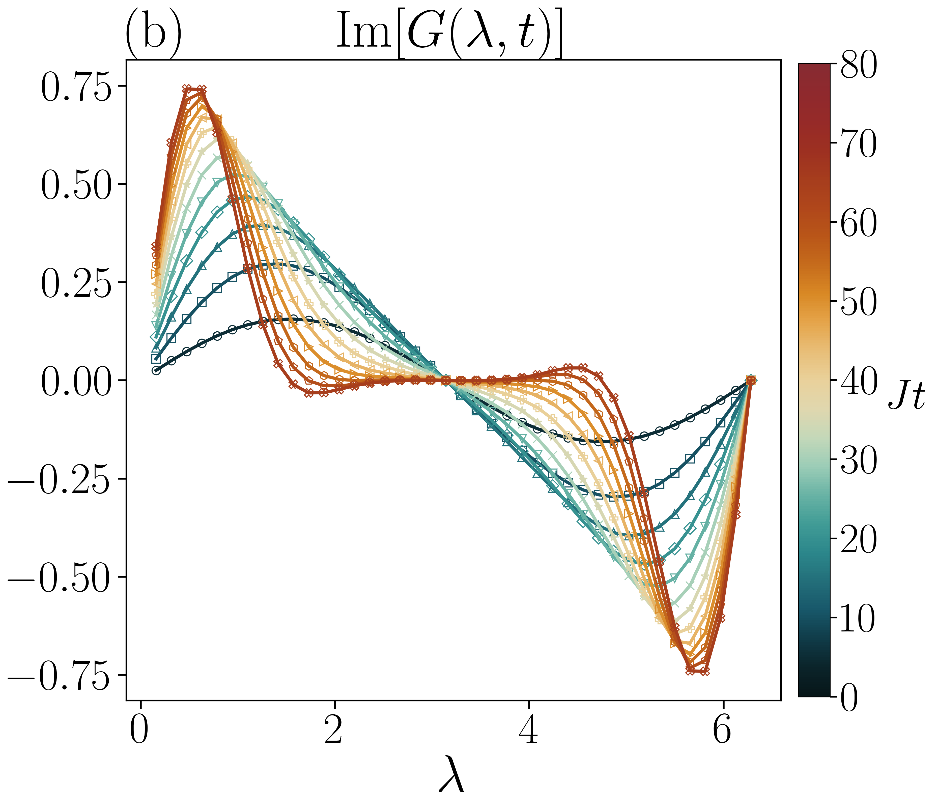
In this section, we present the quantum generating function as a function of . In Fig. S2(a) and (b), we plot both the real and imaginary part of the generating function respectively, by varying between at different time snapshots. In Fig. S2(c), we present the corresponding probability distribution of the injected charge by performing inverse Fourier transform .
IV QGF approach for weakly dephased XXZ chain
In this section, we discuss another setup where the developed QGF approach is efficient for long time dynamics. We consider XXZ and nnn-XXZ chain subjected to local dephasing at each lattice site. The corresponding GKSL equation is given by,
| (S10) |
where is the dephasing strength. The lattice is initialized in the Néel state . Here we are interested in the statistics of the transferred magnetization within a domain of size for a lattice of length (. We choose this domain in the middle of the lattice starting from the site to the site . Therefore, the magnetization operator in the domain and the transferred magnetization operator is . For small dephasing strength , the evolution of the state using the GKSL equation is nontrivial due to the growth of operator space entanglement entropy. Hence we again evolve the counting operator under the adjoint Liouvillian superoperator to obtain and using the QGF, we obtain the moments. All the odd moments of transferred magnetization are zero for this setup. Hence, we compute the second cumulant following Eq. (5) which is same as second moment. This corresponds to the fluctuation of the transferred magnetization in the domain.
In Fig. S3, we plot fluctuations in the transfer magnetization, for domain sizes , and in both the XXZ and nnn-XXZ chains with . To eliminate boundary effects, the total system size is chosen to be much larger than the domain size i.e., in our case. The numerical implementation of the dynamics using the TEBD algorithm, as well as the choice of and , is identical to that employed in Setup-I discussed in the main text. We use a bond dimension of and cutoff . The transport classes can be identified from the dynamics of as: ballistic class correponds to , diffusive class corresponds to , superdiffusive and subdiffusive class correspond to with and respectively. For both models, the early-time behavior of exhibits a quadratic growth in time, . In the XXZ chain, this is followed by a transient ballistic transport and finally diffusive dynamics due to the presence of dephasing. In contrast, the nnn-XXZ chain does not display a ballistic regime beyond the initial quadratic growth and instead exhibits diffusive dynamics at later times.

