Cavity Solitons
W.J. FIRTH and G.K. HARKNESS
Department of Physics and Applied Physics,
University of Strathclyde,
Glasgow G4 0NG, Scotland
A driven optical cavity containing a nonlinear medium can support stable, soliton-like objects, bright non-diffracting spots of light on a uniform background. Importantly, the nonlinear medium need not support ordinary (propagating) spatial solitons, and cavity solitons have been both predicted and observed in a saturable absorber, and predicted to even exist in self-defocusing media. The history, present status, and physical interpretation of such cavity solitons is reviewed. Recent research predicts cavity solitons in semiconductor cavity models with properties interesting for applications to optical information processing. Cavity solitons are natural ‘bits’ for spatial information, possessing both robustness and plasticity, and some potential applications of their unique properties are mentioned.
Introduction
Optical solitons are pulses (or beams) of light in which nonlinearity counter-balances dispersion (or diffraction), leading to a robust structure which propagates without change of form. Strictly speaking, true solitons are exact solutions of integrable nonlinear partial differential equations, but in nonlinear optics mathematical nicety is often foregone in favour of physical robustness. Thus the term ‘soliton’ is increasingly used for any pulse or beam in which dispersion and/or diffraction is compensated on the average by nonlinearity.
Many interesting spontaneous spatial structures have recently been predicted and/or observed in nonlinear optical systems[1]. Among such structures are localised bright spots in driven optical cavities [2, 3, 4, 5, 6, 7, 8, 9, 10, 11, 12, 13, 14, 15, 16, 17, 18, 19, 20, 21, 22, 23]. They share some properties with spatial solitons, counterparts of the soliton pulses being developed as ‘bits’ for long-haul fibre-optic communications, and we will refer to them as cavity solitons. Such structures could be natural ‘bits’ for parallel processing of optical information, especially if they exist in semiconductor micro-resonators. Recent work by the authors and others [16, 17, 19] are very encouraging in that respect.
In this paper we briefly review the history and underlying nonlinear optics of cavity solitons. We then describe in more detail some models which show these soliton-like structures. It is somewhat paradoxical that stable cavity solitons can exist in media with properties different from, even opposite to, those required for Kerr solitons. We therefore consider several candidate physical interpretations of these structures: ‘soliton-in-a-box’, ‘self-trapped switching wave’, ‘pattern element’, and ‘local nonlinear resonance’. We examine the perturbation eigenmodes of the cavity solitons in a sample system, to see whether their shape and nature helps us to reach a global interpretation of these solitons. These eigenmodes also give information on the soliton’s stability and response to external influences such as noise, neighbouring solitons or phase gradients of the holding (or control) field. This leads a discussion of the applications of cavity solitons, which have also been called ‘optical bullet-holes’ (OBH) because they can be created by localised pulses (bullets) of light[8], and can thus be used to store images or information – Fig. 1 shows a cartoon version of such a system. The ability to control and manipulate these solitons offers potential advantages over competing systems, and we speculate about device ideas which might capitalize on these advantages.

Rather than an exhaustive review of the field, this article is subjective, concentrating on our own work. We hope, however, that it succeeds as an overview, if not a review, and we have tried to use our own work primarily to illustrate points of general relevance, without dwelling on their detailed description.
History
The story of cavity solitons can perhaps be divided into three Ages: the Stone Age, the Space Age, and the Information Age. The Stone Age lasted roughly until 1990. During it a few pioneers[2, 3, 4] considered relevant spatial phenomena in cavities. A special journal issue[24] ended that stage, and roughly marks the transition into the Space Age. In the Space Age several favourable circumstances combined to stimulate a huge expansion of interest in spatio-temporal nonlinear optics. Workstation development made dynamical simulation of two-dimensional field patterns widely available. In addition, simple mean-field models of such systems provided a convenient framework which readily matched on to studies of pattern formation in fluids and other fields. A later special issue, in 1994, [1] shows how dramatically the field changed in just a few years. This special issue includes some papers predicting mean-field cavity solitons[12, 13], a trickle which has become a flood in the last few years. As yet the Information Age has barely dawned: in it the emphasis will switch from mere existence of cavity solitons to their engineering and applications.
The history of optical cavity solitons probably began with the seminal paper of Moloney and co-workers[2], who used split-step FFT methods to simulate transverse effects in optical bistability (OB)[25, 26]. The model system was a ring cavity, driven by a gaussian beam, and containing a self-focusing Kerr-like medium. The field was propagated around the cavity, and added coherently to the driving beam at the input beam-splitter. The simulation was one-dimensional (1D), i.e. the intra-cavity field was described by with counting the cavity round-trips. When the input field was ramped up to exceed the OB switch-up threshold, the beam centre switched, and a switching wave moved out, switching up most of the beam (Fig. 2). Then something unexpected happened: a new instability. The interface between the ‘on’ and ‘off’ domains spawned what would now be termed a modulational instability (MI) of the ‘on’ region, which broke up into a set of distinct peaks[2]. These were interpreted as a group of spatial solitons circulating in the medium, perturbed by the output coupling losses and sustained by the input field. Here, therefore, the model was clearly ‘soliton-in-a-box’. Such an interpretation implies that only a medium which could sustain solitons in the bulk can sustain solitons in a cavity.

The original cavity soliton work[2], however, considered a beam either with no solitons, or full of solitons: just two states, and therefore only a one-bit memory in applications terms. McDonald and Firth[4] showed that it was possible to make the individual solitons independently switchable by using a pump beam with a spatially-varying amplitude. They modeled a 20-bit memory of this kind, and also showed that it was possible to switch solitons ‘off’ as well as ‘on’ (with an out-of-phase address pulse)[6].
The other key Stone Age pioneer was Rosanov, who from study of switching waves developed the idea of ‘diffractive autosolitons’ [3], originally in the context of OB. Switching waves between co-existent stable states are known in many fields, such as reaction-diffusion systems. Purely diffusive switching waves have monotonic profiles, and the more stable state simply wipes out the less stable, as was shown in an OB model with pure diffusion[27]. When diffraction is present, however, the switching wave typically has ripples. These can trap other switching waves, and thus two can trap each other. Or, in 2D, one switching wave can bend around and close on itself forming a stable island of one phase surrounded by the other – a diffractive autosoliton (DAS)[3]. Here, then, is a second physical interpretation of cavity solitons: self-trapped switching waves. Note that here there is no requirement for bulk solitons: indeed Rosanov showed that DAS can occur even in a saturable absorber. Nor is OB required: one can have switching waves, e.g. between homogeneous and patterned states, even in the absence of OB.
Rosanov has made many significant contributions to OB and related fields, too many to describe here: the interested reader is referred to his review article[28]. He has also investigated DAS in lasers[29], in which context we remark that we will not deal here with cavity solitons in lasers, nor with the self-imaging oscillators in which single soliton-like structures have been experimentally observed[30, 31].
Mean-Field Models and Cavity Solitons
We now enter the Space Age, characterised by so-called mean-field cavity models, in which alternation of propagation around the cavity with coherent addition of the input field is replaced by a single partial differential equation with a driving term. In the context of spatial pattern formation, this approach is ascribed to the seminal paper of Lugiato and Lefever[32]. Here we give a heuristic derivation of their LL equation, starting from the Nonlinear Schrödinger Equation (NLS). This basically means we are going to consider ‘boxing-in’ a spatial soliton.
Spatial solitons, in a strict sense, exist only for the case of a single transverse dimension, which corresponds to propagation in a planar waveguide. This system is describable to a good approximation by the 1D NLS, one of the best studied and understood of all nonlinear partial differential equations:
| (1) |
Here the first and second order derivatives describe propagation and diffraction respectively, while the term in describes the Kerr effect. This dimensionless form of the NLS is able to describe nonlinear waves in many areas of science[33]. It has a set of ‘soliton’ solutions, which are filaments or pulses of hyperbolic secant shape. The simplest of these is the ‘single soliton’, which in these scaled units has the rather simple formula:
| (2) |
Note that the amplitude and shape propagate without distortion or dispersion, because the z-dependence is just a phase rotation. Though the NLS is idealised, in real optical media soliton-like solutions persist when the NLS is perturbed by inevitable complications such as gain or absorption loss.
A further important idealisation of the NLS is that it assumes an infinite nonlinear medium. Real nonlinear optical media have finite dimensions and, except in glass fibre, solitons can rarely propagate more than a few centimetres before running out of material. This, perhaps, makes it natural to put mirrors around the medium, confining the soliton into a finite slab of material. With perfect reflection and zero absorption, one could indeed confine a soliton in a box. Real mirrors and materials are lossy, but we can make good the loss by ‘feeding’ the caged soliton with an input field. We are thus led to consider a perturbed NLS:
| (3) |
We have added three terms on the right side of the NLS, all small if is. The first is just a linear loss (), and the last is the driving field needed to sustain against that loss. Less obvious is the middle term, in , but we must remember that coherent light confined between mirrors lies within an optical cavity, and so the response to the driving field will strongly depend on whether or not it is in resonance with the cavity. Hence, therefore, we need , the cavity mistuning (if we ignore the left side of (3), then , showing a Lorentzian resonance in ). There is one further change from the NLS: propagation (in ) has now been replaced by evolution (in ). This is natural: the soliton is now in a box, and not going anywhere.
In the limit Eq. (3) recovers the NLS, with a soliton solution of sech-profile in , time independent except for a phase rotation. We might expect, therefore, that for finite it has sech-like cavity soliton solutions for suitable , and indeed it has. It is usual to consider to be a plane wave, independent of and , in which case the soliton sits on a homogeneous non-zero background field .
If we instead set , as we henceforth do, we get the Lugiato-Lefever (LL) equation, which was originally introduced [32] as a model for pattern formation. Note that in the LL equation time is scaled to the cavity loss time. Having removed in this way, to recover the NLS we should now take the limit . The LL equation can also be considered as a ‘mean-field’ model for OB with transverse effects. Mean-field because it is usually derived by assuming a high finesse, so that the cavity field is approximately constant along the cavity axis. The high finesse allows the Airy function response of the cavity to be approximated by a single longitudinal mode, giving the Lorentzian resonance mentioned above. For a plane-wave pump, the plane-wave cavity field obeys , which is three-valued for , showing that the model exhibits OB[32]. In fact, Lugiato and Lefever showed that is stable if , but usually unstable because of spontaneous pattern formation above that threshold[32]. We can now confess that Fig. 2 was generated by simulating the LL equation (for , for (a) and for (b) and (c)), rather than the original full model of Moloney et al.[2]. The strong similarity to the behaviour of the full model shows how such mean-field models can capture the essential features of a full cavity model while being both cheaper to simulate and easier to analyse.
Before developing the theme of mean-field models, it may be worthwhile to describe an important result which shows that cavity solitons can have properties beyond those of propagating spatial solitons. It is well known that the 2D NLS has a cylindrically symmetric soliton-like solution , but that it is unstable, either diffracting away or collapsing to a singularity[33]. What about the cavity equivalent? Firth and Lord[9] found stationary solutions to the 2D LL in the form . For these cavity solitons is plotted against in Fig. 3, for various values of . The solution curve is typical of cavity solitons, forming a loop coexisting with the homogeneous background solution (here ), in the range where the latter is stable.

Our present interest is in the stability of these cavity soliton solutions. As might be expected, the lower branch of the loop is always unstable, but the upper branch may be stable[10]. The domain of stability is shown in Fig. 4, where , the real part of the most unstable perturbation eigenvalue of the upper-branch cavity soliton solution, is shown as a contour plot in the () plane. The stable domain is small, vanishing as is increased - recall that the NLS limit is . Direct simulation confirms the stability analysis. A perturbed cavity soliton exhibits damped oscillations in the stable domain, which become undamped as is increased and the stability boundary crossed. For large the cavity soliton either decays or gets very narrow, suggestive of collapse[9], much as the bulk material solitons do.

Thus we find stable 2D cavity solitons in the Lugiato-Lefever mean-field model, a behaviour qualitatively different from its bulk-medium equivalent. Even if the stable domain is quite small, it perhaps encourages us to look more closely at the LL equation, to see which features we can vary, and which we should maintain, in exploring the world of cavity solitons. Comparing our version of the LL equation to the NLS, we note that the time derivative, and all three terms on the right side, are features associated with the cavity, and thus ought to be maintained. This leaves the diffraction term, and the nonlinearity, as terms we can play with. We already modified the diffraction term when we considered the 2D cylindrically symmetric Kerr cavity solitons. We can go further, by having a true 2D diffraction, and can even add dispersion to make ‘3D’ cavity solitons[23]. Or we can replace diffraction with dispersion, and consider e.g. fibre cavities, where Mitschke and co-workers[15] have found evidence of soliton-like structures in synchronously-pumped fibre loops, and Wabnitz[5] has examined data storage issues. We have assumed a simple cavity with planar mirrors: a nonlinear medium placed within a curved-mirror cavity can be described using a generalised mean-field model involving terms in e.g. , dependent on the ABCD matrix of the cavity[34]. We will not consider such cases[30, 31] here.
The nonlinearity offers great scope for variation. Perhaps the obvious generalisation from the Kerr nonlinearity is to a two-level atom-like response, which becomes Kerr-like far from the atomic resonance[3, 7, 8]. In particular, we will consider the converse of the Kerr limit, namely exact atomic resonance, in which the medium is simply a saturable absorber, with neither a nonlinear nor even a linear refractive index contribution. Again we will find stable, robust cavity solitons, again in a medium with no bulk spatial solitons[8]. A further generalisation is to consider a nonlinearity mediated by a material excitation. This opens up the further possibility that the medium can have its own dynamics and spatial (usually diffusive) coupling. Semiconductors are particularly interesting among such media, and it has been shown[17] that cavity solitons extend to semiconductor models, even in the presence of such ‘soliton-antagonistic’ effects as diffusion and a measure of self-defocusing. Perhaps even more surprisingly, Michaelis et al. [19] found bright solitons in a cavity model with a purely-defocusing, diffusive saturable Kerr medium, such as is found in semiconductors just below the band edge. A different approach is to couple several optical fields through, for example, a nonlinearity. This has been shown in mean-field models to support cavity solitons in both second-harmonic-generation (SHG)[18] and optical parametric oscillator (OPO)[14, 20, 21] configurations.
These cited examples may be just the beginning of an exploration of cavity solitons in a wide range of configurations and media. We will not attempt to detail the cited papers, or to speculate on future developments. What may be worthwhile, however, is to discuss possible physical interpretations of these structures, both because their existence is sometimes counter-intuitive and as a guide to future theory and experiments. We have already considered ‘soliton-in-a-box’ and ‘self-trapped switching wave’. The other pictures mentioned in the Introduction were ‘pattern element’, and ‘local nonlinear resonance’. We now flesh out these pictures, using the saturable absorber cavity as example system[8].
This system is modeled by a modified LL equation in which the Kerr nonlinearity is replaced by a two-level saturable absorption. This takes the form, after appropriate scaling:
| (4) |
The new parameter can be regarded as the density of the saturable medium, expressed in terms of absorptivity. The field, and thus the intensity of the homogeneous solution , is scaled to the saturation intensity. As is well known[26] can become unstable provided , either through OB or, if transverse effects are considered[35], through spatial modulational instability leading to pattern formation[36]. The transverse wave vector of the favoured pattern obeys , which shows immediately that patterns form only in a detuned cavity, and furthermore only if the mistuning is negative. It was shown in[36] that this relation has the simple physical interpretation that the pattern is a ‘tilted-wave resonance’, in which the transverse wave vector just compensates for the cavity mistuning. It was also shown that the favoured pattern is hexagonal.
Now we consider cavity solitons in this model. The profile of a cavity soliton found by direct simulation of the pde (4) is shown in Fig. 5, inset to a plot of its field in the phase plane (note that it lies wholly in the positive quadrant, so there is no significant phase variation associated with the soliton). The continuous line in Fig. 5 is the same solution found by direct radial integration of the time-independent equation for . These phase plots are seen to closely follow that of the hexagonal pattern which coexists with the cavity soliton at these parameters. The plots deviate at the lower left, where the soliton asymptotes to while the hexagon spike must match on to the periodic hexagonal pattern. Fig. 5 essentially defines the ‘pattern element’ interpretation: the soliton as an isolated hexagon spike. Indeed in this example, and by experience in general, cavity solitons are found only for parameter ranges where a stable pattern (usually hexagonal in 2D) also exists. We should point out, however, that we know of no analytic proof of this conjecture applicable to all the cavity soliton models mentioned here. Since switching waves can involve patterns as well as homogeneous solutions, one could also interpret this soliton as a self-trapped switching wave between the hexagonal and the flat state.
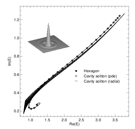
There is a fourth interpretation, however, linked to the ‘tilted-wave’ interpretation of the patterns. Suppose that the curvature of the field profile at the soliton’s centre allows the Laplacian term to cancel the mistuning term due to . Then the cavity is (locally) brought into resonance, bleaching the medium, and making a ‘hole’ in the spatial profile of the absorption. This is equivalent to a gain guide, which confines the beam, activating the Laplacian term , and so on, forming a self-consistent feedback loop. This ‘local nonlinear resonance’ interpretation seems to include some aspects of the other three pictures: for example, one could view the hexagonal pattern as a close-packed collection of local resonances. Note that the local nonlinear resonance picture stresses key features: the cavity (!), and the need for it to be off-resonance in the linear limit. It thus contrasts with ‘soliton-in-a-box’, where the cavity merely keeps the soliton supplied with medium. Our other two pictures lie somewhere in between.
One way to investigate the relative validity and utility of these pictures is to look at the perturbation response of cavity solitons. We have already said that cavity solitons are stable, but the shape and nature of their least stable eigenmodes should give information on their nature via their response to perturbations. For example, in a ‘self-trapped switching wave’ model of the soliton one might expect a prominent eigenmode corresponding to un-trapping.
Investigations of these questions are in at a very early early stage. Here we outline some preliminary results, again for the saturable absorber cavity solitons, and only in one transverse dimension. These results may not be typical, of course, but we believe that they already suggest that this approach has much to contribute to the physics and applications of cavity solitons.
Stationary Solutions and Stability
For convenience, we rewrite equation (4) in terms of the variable , where :
We look for stationary solutions () to this equation in one spatial dimension, , by discretising in space. We thus obtain a large set of coupled nonlinear equations. We use a Fast Fourier Transform (FFT) to compute the spatial derivatives in Fourier space. This gives high accuracy (of order , the number of spatial grid points). From suitably chosen initial conditions a Newton method is used to find solution(s) of the set.
The benefit of such a procedure over the more usual direct simulation of the pde is that it can yield all the stationary solutions, not just those which are dynamically stable. Further, any solution’s stability is determined by the eigenvalues and eigenvectors of the Jacobian matrix obtained by linearising around it, a matrix which is already calculated for use in the Newton method. If any of the eigenvalues of the Jacobian have a positive real part then the solution is unstable. The associated eigenvector gives the spatial profile of the mode, whether stable, unstable,or neutral.
By this technique, we have computed a number of solutions and their stability. Some typical results are shown in Fig. 6.

Of particular interest is the solution branch corresponding to a singly-peaked localised state (labelled ), i.e. the cavity soliton. Just as for the Kerr cavity case in Fig. 3, this cavity soliton co-exists with the homogeneous background solution and the pattern state, in this case rolls (these would correspond to stripes in 2D). There also exist solutions which are like multiple cavity solitons, , , etc.

Turning now to the stability of the cavity soliton, as mentioned this information is readily derived from the solution method used. The eigenfrequencies (imaginary parts of the eigenvalues) are responsible for the response spectrum of the cavity soliton to perturbations. Driving an eigenmode will make the cavity soliton oscillate at the driving frequency, with an amplitude which will be maximum when the driving field resonates with the mode, with the height and width of the resonance determined by the real part of the eigenvalue. For the present problem, the spectrum is very simple: the modes with smallest damping all have real eigenvalues. This means that, despite the fact that the pump field is detuned by from the empty-cavity resonance, the perturbation response of the loaded cavity is primarily at the pump frequency (nonlinear resonance).
We plot as a function of the intensity in Fig. 7 some of the perturbation eigenvalues of the cavity soliton, to be precise the eight most ‘dangerous’ ones, i.e. with least-negative eigenvalues. From the plot we see that the cavity soliton is stable over the approximate range . Note that there always exists a zero eigenvalue. It occurs because of the translational symmetry in the -direction. Its existence is of great importance for applications, as will be discussed in the next section. As is common for other solitons, this neutral mode has an eigenvector which is the gradient of the state itself, because the gradient operator is the generator of translations.
At the lower limit of this range in , a second eigenvalue approaches zero, and the cavity soliton loses stability at its existence limit (see Fig. 6). The corresponding eigenvector is shown in panel (b). It is highly localised on the cavity soliton, and this mode thus strongly supports the picture of a cavity soliton as a ‘local nonlinear resonance’. As is increased, it can be seen from Fig. 7 that this mode becomes more damped (but its form changes only slightly). At about this eigenvalue seems to undergo an anti-crossing with that of another mode. The latter mode, in conjunction with a third one, then assumes dominance, until, at the upper limit of its range in , the cavity soliton loses stability to a degenerate pair of modes, with eigenvectors shown as full and dotted lines in panel (c). The instability occurs where the CS branch collides with the 1.5CS branch. These eigenvectors seem to be of switching-wave type, being located where a neighbour soliton would be expected to appear. This type of mode supports the ‘trapped switching wave’ picture. Incidentally, the modes associated with the other eigenvalues in Fig. 7 are extended, pattern-like states. The damping of such states is expected to weaken as the homogeneous solution becomes less stable on approach to the MI threshold (, see Fig. 6) [8].
Thus the eigenmodes of the cavity soliton for this model seem to suggest that it is primarily a local nonlinear resonance at low powers, but that at the upper end of its range, it becomes more akin to the self-trapped switching wave picture. For applications, one might want to work in the most stable region, where the two modes cross over. At that point, the correct interpretation is far from clear: trapped switching wave? local nonlinear resonance? a bit of both?
Applications
Arrays of cavity solitons may have applications in parallel information processing[16]. They can be created at any location by a suitable address pulse, are non-diffracting and dynamically stable, all of which makes them suitable ‘bits’ for image or data capture, storage and processing. This has been demonstrated numerically in [8] and confirmed in a prototype experiment[16]. A simple binary memory array, such as implied by Fig. 1, is unlikely to to be competitive with electronic storage. Cavity solitons, however, also offer functionalities which are beyond any micro-structured material array, whether optical or electronic. In particular, they can be optically manipulated, e.g. by imposing a spatial phase profile on the driving field. Processing schemes which take advantage of their unique properties may avert the unequal competition with silicon which has plagued other all-optical processing schemes.
The plasticity of cavity solitons can be linked to the ‘neutral mode’ identified in the previous section, which is associated with the translational invariance of the underlying equations defining the cavity solitons. Any perturbation to the pump field which has a finite gradient at the soliton location will couple to the neutral
mode and cause the soliton to move. The speed of the motion is essentially proportional to this gradient, and so the soliton will continue to move until it reaches a gradient-free location. This has implications for the response of the cavity solitons to noise and to any stray gradients, and also for interaction between solitons. Here we will consider only its use to control the motion and location of the solitons through the spatial phase profile of the pump field. It is as though the solitons inhabit a ‘landscape’ determined by the phase of the holding (control) field, a landscape in which they move in response to phase gradients. Thus a simple memory array[8] consists of a regular landscape of ‘hills’ and ‘valleys’, with the solitons attracted to the peaks. Unlike one formed from machined pixels, however, this landscape is reconfigurable by changing the phase profile of the control field. This allows cavity soliton bits to be manipulated, by either global or local reconfigurations of the control field. No such manipulation is possible in material arrays, whether of optoelectronic pixels or in silicon. This plasticity opens up possibilities for novel processing functions and applications such as a ‘soliton carousel’, a ‘soliton assembly-line processor’ and a ‘zoom memory’. One can also expect useful applications in digital image processing, for example in feature extraction.
Conclusion
We have discussed a class of stable soliton-like structures predicted to exist in driven optical cavities containing any of a wide variety of nonlinear materials. This class includes semiconductor micro-resonators, which is promising for possible applications of these cavity solitons. They can be formed into two-dimensional arrays of information bits which can be written, stored, read, erased [11], and spatially manipulated in various ways. They can thus act as the basis of a new kind of all-optical parallel processor, with functionalities not available to other processing and storage devices in information technology.
The first experimental verifications of these solitons have been made [16], while they have been found theoretically in quite a wide variety of cavity systems containing a nonlinear optical medium. We believe that in the coming years they will find an important role both in optics and in optoelectronic technology.
Acknowledgements
We thank Angus Lord and Andrew Scroggie for important contributions to this paper, which is based on an invited talk delivered by WJF at the Nonlinear Guided Waves ’98 conference in Victoria, Canada, in April 1998. WJF would like to thank the organisers and sponsors of that meeting. GKH acknowledges a grant from the RDF of the University of Strathclyde. We thank our partners in PASS, and its successor project PIANOS, for many helpful discussions and insights.
References
- [1] Lugiato L A (editor), Special issue on “Nonlinear Optical Systems, Chaos, Noise”, Chaos, Solitons & Fractals 4(1994)1307
- [2] McLaughlin D W, Moloney J V & Newell A C, Phys Rev Lett, 51(1983)75. See also Moloney J V & Newell A C, Nonlinear Optics, (Addison-Wesley, Redwood City), 1992 Fig. 5.16, p225, and associated text.
- [3] Rosanov N N & Khodova G V, Opt Spektrosk, 65(1988)1375; J Opt Soc Am B, 7(1990)1065.
- [4] McDonald G S & Firth W J, J Opt Soc Am B, 7(1990)1328.
- [5] Wabnitz S, Opt Lett, 18(1993)601.
- [6] McDonald G S & Firth W J, J Opt Soc Am B, 10(1993)1081.
- [7] Tlidi M, Mandel P & Lefever R, Phys Rev Lett, 73(1994)640.
- [8] Firth W J & Scroggie A J, Phys Rev Lett, 76(1996)1623.
- [9] Firth W J & Lord A, J Mod Optics, 43(1996)1071.
- [10] Firth W J, Lord A, & Scroggie A J, Phys Scripta, T67(1996)12.
- [11] Brambilla M, Lugiato L A & Stefani M, Europhys Lett, 34(1996)109.
- [12] Tlidi M & Mandel P, Chaos, Solitons & Fractals, 4(1996)1475.
- [13] Scroggie A J, Firth W J, McDonald G S, Tlidi M, Lefever R & Lugiato L A, Chaos, Solitons & Fractals, 4(1996)1323.
- [14] Longhi S, Opt Lett, 21(1996)860.
- [15] Steinmeyer G, Schwache A & Mitschke F, Phys Rev, E53(1996)5399.
- [16] Weiss C O et al, ESPRIT LTR Project 21112 PASS: Report.
- [17] Brambilla M, Lugiato L A, Prati F, Spinelli L and Firth W J, Phys Rev Lett, 79(1997)2042.
- [18] Etrich C, Peschel U & Lederer F, Phys Rev Lett, 79(1997)2454.
- [19] Michaelis D, Peschel U & Lederer F, Phys Rev, A56(1997)R3366.
- [20] Staliunas K & Sanchez-Morillo V J, Opt Commun, 139(1997)306.
- [21] Tlidi M, Mandel P & Haelterman M, Phys Rev, E56(1997)6524.
- [22] Michaelis D, Peschel U & Lederer F, NLGW’98 paper NWA3 (unpublished).
- [23] Tlidi M & Haelterman M, PINOS Euroconference 1998 (unpublished).
- [24] Abraham N B & Firth W J, J Opt Soc Am B, 7(1990)951.
- [25] Gibbs H M, Optical Bistability – Controlling Light with Light, (Academic Press), 1985.
- [26] Lugiato L A, Progress in Optics (Wolf E, ed.), XXI(1984)69 (North Holland).
- [27] Firth W J & Galbraith I, IEEE J Quant Elec, QE-21(1985)1399.
- [28] Rosanov N N, Progress in Optics (Wolf E, ed.), XXXV(1996)1.
- [29] Rosanov N N, Fedorov S V & Khodova G V, J Exp Theor Phys, 107(1995)376; Rosanov N N, Fedorov S V & Khodova G V, Physica D, 96(1996)272.
- [30] Bazhenov V Yu, Taranenko V B & Vasnetsov M V, Proc. SPIE, 1840(1992)183; Taranenko V B, Staliunas K & Weiss C O, Phys Rev, A56(1997)1582.
- [31] Saffman M, Montgomery D & Anderson D Z, Opt Lett, 19(1994)518.
- [32] Lugiato L A & Lefever R, Phys Rev Lett, 58(1987)2209.
- [33] Newell A C, Solitons in Mathematics & Physics, (Philadelphia: SIAM), 1987.
- [34] Dunlop A M, Firth W J & Wright E M, Opt Commun, 138(1997)211.
- [35] Lugiato L A & Oldano C, Phys Rev, A37(1988)3898.
- [36] Scroggie A J & Firth W J, Europhys Lett, 26(1994)521.