Linear and Nonlinear Latent-Space Reduced-Order Models for the
Rayleigh–Taylor Instability
Abstract
We use a large database of direct numerical simulations to investigate the transition of the Rayleigh–Taylor instability to turbulence and its evolution toward a late-time self-similar regime. In addition to tracking the growth of the mixing layer through the mean heavy-fluid concentration profile, we analyze one-dimensional profiles of turbulent kinetic energy and dissipation, two key quantities in classical turbulent-mixing models. We consider two reduced-order modeling strategies that differ in where nonlinearity is introduced: either in the construction of the latent space or in the description of its temporal evolution. The first method uses a linear encoder–decoder obtained using Proper Orthogonal Decomposition (POD), with nonlinear reduced dynamics learned by a physics-informed neural network (PINN). The second uses a nonlinear encoder–decoder learned by an autoencoder, while constraining the latent dynamics to remain linear and satisfy physical constraints. Both approaches achieve satisfactory performance in reconstructing, interpolating, and extrapolating the dynamics of the Rayleigh–Taylor instability.
Keywords: Rayleigh–Taylor instability, Turbulence, Reduced-order modeling, POD, PINNs, LaSDI, Autoencoder.
1 Introduction
The Rayleigh–Taylor instability (RTI) (Rayleigh, 1882; Taylor, 1950), which develops when a heavier fluid lies above a lighter fluid in a gravitational field, is an efficient mechanism for converting potential energy into turbulent mixing (Zhou, 2017a; Zhou, 2017b). In the context of inertial confinement fusion (ICF), this instability develops at the interface between the ablator and the fuel, leading to mixing that causes additional cooling and weakens fusion reactions (Lindl, 1995; Betti and Hurricane, 2016; Remington et al., 2019; Zhou et al., 2025).
Direct numerical simulations of turbulent mixing flows remain scarce and costly in many applications, including the Rayleigh–Taylor instability, despite ongoing advances in computational resources. This forces the engineering community, and in particular researchers developing predictive models for ICF, to rely on more computationally efficient approaches, such as Reynolds-Averaged Navier–Stokes (RANS) models.
Developing a consistent RANS model for turbulent flows driven by RTI remains a formidable task, not only because the large scales of RTI are highly anisotropic, but also because the flow is strongly unsteady, transitioning from a laminar to a turbulent regime while retaining some memory of the initial conditions.
These features challenge classical RANS assumptions, such as spectral equilibrium within the turbulent cascade or the Boussinesq approximation for the Reynolds stress tensor. This motivates the development of surrogate and reduced-order models (ROMs) capable of extracting the essential dynamics from high-fidelity simulations while remaining computationally affordable.
Beyond their use as computational accelerators, reduced-order and surrogate models have become essential tools for the analysis and modeling of complex fluid systems. Their low computational cost enables large-scale parameter explorations, uncertainty quantification, flow control, and optimization studies that would be prohibitively expensive with high-fidelity simulations alone (Noack et al., 2011). In turbulence modeling, surrogates also provide a convenient framework for data assimilation, model calibration, and the development of improved closure models by disentangling parametric and structural modeling errors (Creusy et al., 2026). Such applications have motivated the development of reduced representations capable of accurately reproducing the essential dynamics of high-dimensional systems while remaining computationally tractable.
Many nonlinear dynamical systems encountered in fluid mechanics involve an extremely large number of degrees of freedom. Nevertheless, their evolution is often effectively confined to a low-dimensional manifold. Reduced-order models exploit this property by seeking compact representations that retain the essential features of the underlying high-dimensional dynamics while drastically reducing the computational complexity. The construction of an efficient ROM therefore relies on two fundamental ingredients: the identification of a suitable low-dimensional representation of the flow structures and the development of an accurate model for the dynamics evolving on this reduced manifold.
Modal decomposition techniques provide a natural framework to address the first of these challenges. By separating spatial and temporal dependencies, they represent the flow field as a superposition of modes weighted by time-dependent amplitudes. Such approaches have become central tools in fluid mechanics for identifying coherent structures, analyzing nonlinear dynamics, and constructing low-dimensional models (Taira et al., 2017). Among them, the Proper Orthogonal Decomposition (POD), introduced through the method of snapshots by Sirovich (Sirovich, 1987) and extensively reviewed by Berkooz et al. (Berkooz et al., 1993), remains one of the most widely used reduction techniques owing to its optimality in representing a dataset with a low-dimensional linear basis.
The second challenge consists in modeling the evolution of the reduced variables. A classical strategy relies on Galerkin projection of the governing equations onto the POD basis, yielding a dynamical system for the modal amplitudes. However, the accuracy of such models relies on the adequacy of the reduced basis to describe the underlying dynamics. Additional modeling strategies may therefore be required, as illustrated by Noack et al. (2003), who introduced a shift mode to improve the representation of transient dynamics in the periodic cylinder wake by accounting for the displacement between the steady solution and the averaged flow.
Despite their success, classical POD-Galerkin models suffer from several well-known limitations. First, the POD basis is constructed from a specific ensemble of snapshots and therefore defines a reduced space associated with a particular dynamical regime and set of physical parameters. As a consequence, the POD eigenspace itself may change when control parameters are varied, reducing the predictive capability of the resulting ROM. This lack of robustness away from the reference configuration was already emphasized by (Deane et al., 1991). Such a dependence on the training conditions becomes particularly restrictive for parametric studies, where the objective is to interpolate or extrapolate the system dynamics over a broad range of physical parameters.
Second, the assumption that a fixed set of modes can efficiently represent the flow becomes questionable for transport-dominated phenomena (Rowley and Marsden, 2000). Because the spatial modes are fixed, advected or moving coherent structures often require a large number of modes to be represented accurately, thereby reducing the efficiency of linear modal decompositions. This issue has motivated the development of alternative nonlinear representations and machine-learning-based mappings capable of representing transport-dominated flows more efficiently (Kim et al., 2020).
Third, the truncation of the governing equations introduces unresolved interactions between retained and discarded modes, raising important closure and stability issues. The long-time behavior of truncated POD-Galerkin models remains a challenging issue, as emphasized in (Ma and Karniadakis, 2002). More generally, accurately reproducing the energy transfer between resolved and unresolved scales remains one of the major challenges of projection-based ROMs and requires suitable closure strategies (Callaham et al., 2023).
Recent advances in machine learning have opened new perspectives for overcoming these limitations by learning reduced representations and reduced dynamics directly from data (Brunton et al., 2020). Deep-learning-based approaches have been proposed to improve closure modeling and long-time predictive capabilities of reduced-order models. For example, the Complemented Deep Reduced-Order Model (CD-ROM) combines projection-based techniques with neural networks to represent unresolved dynamics and improve predictive robustness (Menier et al., 2023). Similarly, physics-informed neural networks (Raissi et al., 2019) have recently been employed to construct surrogate models that enforce governing equations and physical constraints while maintaining low computational costs (Thévenin et al., 2025b; Volk et al., 2025).
Machine learning has also enabled the development of nonlinear latent representations through autoencoders. From a theoretical perspective, linear autoencoders are closely related to POD and recover the same optimal subspace under appropriate assumptions (Bourlard and Kamp, 1988; Bourlard and Kabil, 2022; Bousquet et al., 2026). More generally, autoencoders may be interpreted as nonlinear extensions of POD in which the data are projected onto a nonlinear manifold rather than onto a linear subspace (Bousquet et al., 2025). Such embeddings provide an accurate framework for representing strongly nonlinear dynamics (Champion et al., 2019; Messenger et al., 2025). Combined with latent-space dynamics identification techniques (LasDI), they further enable the construction of parametric surrogate models by learning the evolution equations directly in the nonlinear latent space (Bonneville et al., 2024; Farenga et al., 2025).
The combination of encoders with dynamical systems identification has led to a new generation of reduced-order models. Neural networks have been employed to correct truncation errors within POD subspaces while simultaneously learning additional latent dynamics (Lepage et al., 2025). More generally, the Koopman operator framework (Koopman, 1931; Koopman and v. Neumann, 1932), provides a powerful perspective by seeking approximately linear representations of nonlinear dynamics in appropriately chosen observables. Recent works have combined autoencoders and Koopman theory to identify finite-dimensional latent spaces in which nonlinear systems evolve approximately linearly (Lusch et al., 2018). Similarly, (Champion et al., 2019) proposed to identify governing ordinary differential equations directly in the latent space of an autoencoder, although the resulting dynamics are not parameterized with respect to physical control parameters.
Finally, recent developments in scientific machine learning increasingly blur the distinction between purely physics-based and purely data-driven approaches (Vinuesa et al., 2026). Hybrid strategies that combine physical knowledge with data-driven representations offer promising avenues to construct compact, interpretable, and robust surrogates for complex dynamical systems.
The present work uses this hybrid approach. We compare two reduced-order modeling strategies for the evolution of the one-dimensional profiles of a Rayleigh–Taylor flow that transitions to turbulence. Both strategies share the same overall pipeline: an encoding-decoding step that reduces the profiles to a low-dimensional representation, followed by a model of the temporal evolution of that representation. They differ in which of the two stages is allowed to be nonlinear. The first strategy encodes and decodes the profiles linearly, through a Proper Orthogonal Decomposition basis. It then learns nonlinear reduced dynamics with a physics-informed neural network (PINN). The second strategy reverses this choice. The profiles are encoded and decoded nonlinearly, by an autoencoder. The reduced-order dynamics are instead constrained to remain linear, and to satisfy physics-informed constraints. Modeling dynamics in a reduced-order latent space has been standard practice for many decades. This approach is now commonly referred to as Latent Space Dynamics Identification (LaSDI), (Bonneville et al., 2024; Farenga et al., 2025). Under this terminology, both strategies we consider can be seen as particular realizations of LaSDI.
2 DNS dataset for the Rayleigh-Taylor instability
In this section, we describe the theoretical framework underlying the RT database, define the key quantities that we aim to reproduce, and provide insight into the physical phenomena observed in the simulations. The dataset comprises direct numerical simulations spanning a broad range of initial interface perturbations, as introduced by Thévenin et al. (2025b); Thévenin and Gréa (2025). The simulations were performed on a grid of points using the in-house pseudo-spectral code STRATOSPEC (Gréa and Briard, 2019; Briard et al., 2020; Briard et al., 2025a; Briard et al., 2025b).
2.1 Governing equations and nondimensionalization
The present study is conducted within the Boussinesq approximation, which is valid for a small Atwood number , where quantifies the relative density contrast between the two fluids.
The flow is described by the velocity field and the heavy-fluid concentration field . Under these assumptions, their evolution is governed by the incompressible Navier–Stokes and advection–diffusion equations:
| (1a) | ||||
| (1b) | ||||
| (1c) | ||||
where repeated indices are summed over and denotes the Kronecker delta. Equation (1a) enforces incompressibility; Eq. (1b) expresses momentum conservation; and Eq. (1c) governs the advection–diffusion of the concentration field. Here, denotes the reduced pressure, is the magnitude of the gravitational acceleration directed downward along the -axis, and and are the constant kinematic viscosity and molecular diffusivity, respectively. In all simulations, , corresponding to a Schmidt number .
Physical quantities are rendered dimensionless using the characteristic length and time , constructed from the kinematic viscosity and the reduced acceleration :
| (2) |
Hereafter, the quantities are considered dimensionless. This nondimensionalization is particularly important because the surrogate models presented in this work are intended to predict physical quantities across a broad range of conditions, thereby promoting generalizability.
2.2 Initial setup
A complete description of the initial setup used in the simulations is provided by Thévenin et al. (2025b); Thévenin et al. (2025a). The heavy fluid is initially placed above the lighter fluid along the vertical -direction, with the two fluids separated by a diffuse interface. The initial velocity field is zero, and the interface is subjected to a random perturbation. The two-dimensional spectrum of this perturbation is characterized by its mean wavenumber, spectral bandwidth, and mean amplitude. The initial condition can therefore be summarized by four dimensionless parameters: the initial Reynolds number , which characterizes the mean wavelength of the perturbation and the buoyancy strength; the normalized spectral bandwidth ; the mean interface steepness ; and the normalized thickness of the unperturbed diffuse interface.
2.3 Mean fields and turbulent 1D quantities
In the RT simulations, the flow is statistically homogeneous within each horizontal – plane. The instantaneous concentration and velocity fields can therefore be decomposed into their Reynolds averages and corresponding fluctuations as
| (3a) | ||||
| (3b) | ||||
Here, and denote averages over the horizontal plane, whereas and denote the corresponding fluctuations. For the present configuration, the mean velocity vanishes, such that .
At this stage, it is useful to introduce the width of the RT mixing zone, denoted by , which is the primary quantity to be reproduced from the dataset. Following Andrews and Spalding (1990), this width is defined in terms of the mean concentration profile as
| (4) |
The prefactor ensures that coincides with the geometrical thickness of a piecewise-linear mean concentration profile, as is commonly observed in turbulent mixing layers.
Accordingly, the profiles of turbulent kinetic energy and its dissipation rate are defined as
| (5a) | ||||
| (5b) | ||||
In addition to the mean concentration, turbulent kinetic-energy, and dissipation profiles, which are the main quantities of interest in this study, we introduce the vertical component of the turbulent kinetic energy, defined by
| (6) |
The vertical turbulent mass flux and concentration variance are defined by
| (7) | ||||
| (8) |
These additional quantities are used to enforce the physical consistency of the reduced-order models.
2.4 Spatially integrated quantities (0D)
In addition to the one-dimensional profiles, spatially integrated quantities are considered throughout this work. These zero-dimensional observables provide a compact description of the global evolution of the instability. For a generic profile , we define
| (9) |
The zero-dimensional turbulent kinetic energy, dissipation rate, and mass flux are denoted by , , and , respectively.
2.5 Phenomenology of the RT dynamics
The evolution of a Rayleigh–Taylor mixing layer proceeds through several distinct regimes: the linear regime, the weakly nonlinear regime, the transition to turbulence, and, at late times, the self-similar regime (Sharp, 1984). These regimes have been extensively studied; see, in particular, Thévenin and Gréa (2025), who proposed a simple phenomenological model describing their evolution. In this section, we first present the evolution of the zero and one-dimensional quantities and then discuss the late-time scaling laws that underpin the analysis developed throughout this manuscript.
2.5.1 Example of trajectory 0D/1D dynamics
Figure 1 illustrates the temporal evolution of the one-dimensional profiles of the mean concentration, turbulent kinetic energy and its dissipation rate, together with their zero-dimensional counterparts. These quantities form the basis of most Reynolds-averaged Navier–Stokes (RANS) turbulence models.
As the initial multimode perturbation grows, dominant spikes and bubbles develop and subsequently undergo secondary instabilities, ultimately triggering the transition to turbulence. This process is marked by a peak in the dissipation rate, also referred to as an enstrophy blow-up, which reflects a transient imbalance in the transfer of energy across scales. Notably, this phenomenology is highly sensitive to the initial conditions, which are characterized here by the parameters , , , and .
Capturing the dependence of these trajectories on the initial conditions is, therefore, one of the primary objectives of the surrogate model. At late times, the Rayleigh–Taylor mixing layer enters a self-similar regime, whose characteristic scaling laws are examined in greater detail below.

2.5.2 Self-similar scaling
The late-time self-similar regime of Rayleigh–Taylor mixing, which can be anticipated from dimensional analysis (Youngs, 1984), is characterized by a quadratic growth of the mixing-layer width:
| (10) |
where is the asymptotic self-similar growth coefficient, which has been shown to exhibit universal behavior in our database (Thévenin and Gréa, 2025). By contrast, denotes the virtual origin of the self-similar solution. Because it is closely related to the transition to turbulence, remains strongly dependent on the initial conditions. It follows directly that the growth velocity of the mixing layer scales linearly with the shifted time:
| (11) |
Introducing the self-similar coordinate
| (12) |
and appropriately rescaling the various one-dimensional profiles, the resulting quantities are expected to become independent of time and to collapse, at sufficiently late times, onto corresponding self-similar profiles (see also Ristorcelli and Clark (2004)). More precisely,
| (13a) | ||||
| (13b) | ||||
| (13c) | ||||
| (13d) | ||||
| (13e) | ||||
In Fig. 2, we show the collapse of the one-dimensional self-similar profiles obtained from a similar trajectory previously depicted in Fig. 1. As expected, the mean concentration profile, , approaches a nearly piecewise-linear shape, whereas the other turbulent quantities converge toward approximately parabolic profiles.

During the transition to turbulence, near the peak of dissipation, more complex profile shapes may emerge. Localized vortical structures generated by secondary instabilities during the breakup of bubbles and spikes can produce bumps or flattened regions in the one-dimensional profiles near the centerline of the mixing zone. These structural variations are also intended to be captured by the surrogate models.
3 POD-based surrogate modeling framework
This first strategy places nonlinearity in the temporal dynamics rather than in the profile representation. The one-dimensional fields, expressed using the self-similar scaling defined in Eq. (13), are projected onto a truncated Proper Orthogonal Decomposition (POD) basis. This constitutes a linear encoding–decoding step: both the reduction of the profiles to modal amplitudes and their reconstruction are linear operations. The evolution of these amplitudes as functions of time and the initial-condition parameters is then learned by a physics-informed neural network (PINN), which provides an explicitly nonlinear model of the reduced dynamics.
3.1 Physics-regulated POD
We employ the POD to construct a reduced representation of the self-similar profiles defined in Eq. (13). A generic transformed quantity is represented in an -dimensional modal space as
| (14) |
where are the spatial modes and their associated temporal amplitudes. Because the dominant temporal scaling has already been removed, approaches the stationary profile in the self-similar regime and the corresponding modal amplitudes remain bounded at late times. The POD identifies the set of modes that provides the optimal orthogonal basis for a quantity with the norm induced by the inner product
| (15) |
which is defined on the spatial domain for profiles and . We approximate this integral using a Simpson quadrature, yielding a weighted sum on the discrete approximations of and using 201 points.
The POD modes are computed using the method of snapshots combined with singular value decomposition (SVD) (Sirovich, 1987). This decomposition provides the optimal rank- approximation of the snapshot matrix in the sense (Eckart and Young, 1936).
The objective is to identify modes that efficiently represent the complete ensemble of initial conditions considered in the database, rather than a single trajectory. Because the different quantities exhibit distinct spatial structures and symmetries, a common basis would provide no clear reduction advantage and would compromise the optimal rank- approximation obtained for each field separately. We therefore construct an independent POD basis for each quantity, thereby improving reconstruction accuracy for a fixed number of retained modes.
To this end, a snapshot matrix is constructed independently for each rescaled quantity expressed self-similarly from 10,000 profiles uniformly sampled over the trajectories and time steps of the training set. These matrices represent approximately 10% of the available profiles for each quantity.
Self-similar representation
The POD is performed on the rescaled quantities , , , , , and . The transformations defined in Eq. (13) map the expanding physical profiles onto the fixed coordinate and remove their known growth with the mixing length; is scaled in the same manner as .
This formulation prevents late-time snapshots from dominating the POD solely because of their larger physical magnitude. More importantly, the transformed profiles become time independent in the asymptotic self-similar regime. The POD modes can therefore separate the stationary late-time structure from the transient deformations associated with the instability development and transition to turbulence.
Symmetry
Under the weak-density-contrast approximation, the Rayleigh–Taylor instability is statistically symmetric about . Accordingly, , , , , and are treated as even quantities, whereas is treated as odd. Because individual DNS realizations do not satisfy these symmetries exactly, each snapshot is replaced by its appropriate symmetric component before applying the POD.
This preprocessing reduces the effective number of degrees of freedom and guarantees that every profile reconstructed from the POD basis satisfies the required symmetry, thereby preventing spurious asymmetric predictions and preserving physical consistency.
Realizability
Some of the self-similar quantities are positive because they are defined from squared fluctuations (, , , and ). Their low-rank reconstruction should therefore preserve realizability, although a standard POD expansion provides no such guarantee.
To retain a linear SVD-based encoding while enforcing non-negativity after reconstruction, the POD is applied to the square root of these quantities. The resulting representations are
| (16) |
The square-root transformation is applied directly to the sampled self-similar snapshots before the SVD. One POD basis is thus obtained for each of , , , , , and .
No temporal or ensemble mean profile is subtracted before the decomposition. In self-similar variables, the late-time state is stationary but nonzero. Removing the mean would therefore eliminate a substantial part of the asymptotic profile that the ROM is intended to reproduce. Retaining it allows the leading POD mode to represent the stationary self-similar structure, while the higher-order modes describe transient departures from that state.
3.2 Identification of self-similar and transitional modes
The POD framework introduced in the previous section forms the basis of the reduced-order model employed to predict the profile evolution as a function of the initial conditions. To determine an appropriate truncation rank, a modal analysis of the training database is first performed.
The POD is computed from randomly selected self-similar snapshots of the training set. For each quantity, the amplitude associated with the leading mode approaches a nonzero asymptotic value once the self-similar regime is reached, while the amplitudes of the higher-order modes decay. Consequently, the leading mode provides a direct modal representation of the stationary self-similar profile: up to a multiplicative factor given by its asymptotic amplitude, captures the asymptotic profile shape (see Appendix A.1.2).
All POD modes are presented in Appendix A.1, Fig. 10, while the temporal amplitudes of the first two modes for all quantities are shown in Fig. 11.
The temporal amplitudes associated with the leading modes also provide a direct representation of the corresponding zero-dimensional quantities obtained by spatial averaging of the profiles. Consistently with the usual interpretation of POD decompositions, the first mode captures the dominant average structure of the dataset. Indeed, its temporal amplitude times the mixing layer width closely follows the evolution of the corresponding spatially averaged quantity (see Appendix A.1.1), with relative errors around over the entire dataset (about mean error using all modes).
The secondary modes, , display more complex spatial structures, characterized by localized extrema near the boundaries of the mixing layer. Their temporal amplitudes indicate that they are predominantly active during the early stages of the instability (), while they become negligible compared with the leading mode at later times. Moreover, their amplitudes tend to zero in the turbulent regime, suggesting that they play only a minor role in the asymptotic dynamics. A plausible physical interpretation is that these modes capture the initialization phase and the transition towards fully developed turbulence.
The higher-order modes, , exhibit increasingly oscillatory structures that resemble Fourier modes. Their amplitudes remain small throughout the simulations and do not exhibit any clear dependence on the initial conditions . Furthermore, they do not admit an obvious physical interpretation and primarily capture high-frequency fluctuations associated with the stochastic nature of the trajectories, such as phase differences between the initially imposed perturbation modes.
Based on this modal analysis, five modes are retained for , , , , and , whereas four modes are sufficient for the mean concentration . This selection provides a compromise between compactness, physical interpretability, and reconstruction accuracy. The resulting truncation error is evaluated on the test set in Appendix A.2.5, Fig. 13, where it is compared with the complete POD–PINN error.
Summary
To summarize, the construction of the POD modes for each quantity proceeds as follows (also illustrated in Fig. 3):
- 1.
Randomly draw 10,000 profiles of a given quantity, uniformly sampled across trajectories and time steps, to form the snapshot matrix.
- 2.
Express all snapshots in their self-similar form: , , , , , and ; see Eq. (13).
- 3.
Apply a square-root transformation to , , , and to ensure non-negative reconstructions.
- 4.
Enforce the statistical symmetry of the profiles: retain the even component of the turbulent quantities and the odd component of .
- 5.
Perform the singular value decomposition of the snapshot matrix. The POD modes are the columns of the matrix .
- 6.
Six sets of POD modes are obtained, one for each quantity.
- 7.
Retain 5 modes for , , , , and , and 4 modes for .

3.3 Physics-informed surrogate model in reduced space
To exploit the reduced-order representation defined in Eq. (16) and generate profile predictions from arbitrary initial conditions, a surrogate model is required to map the initial parameters to the corresponding temporal POD amplitudes.
This mapping is highly nonlinear, in contrast with the linear encoding-decoding step relating the profiles to their POD amplitudes. Constructing an explicit analytical relation between the initial conditions and the POD coefficients remains challenging.
Moreover, the problem is intrinsically non-unique. The four non-dimensional parameters provide a statistical characterization of the initial perturbation but do not contain information about the phase distribution of the individual perturbation modes. Therefore, different initial perturbations characterized by identical values of may, in principle, lead to different instantaneous evolutions. The surrogate model must therefore learn the dominant statistical trends of the dynamics rather than reproduce the exact trajectory associated with a fully specified initial condition.
To address this challenge, a physics-informed neural network (PINN) framework (Raissi et al., 2019) is introduced to learn the evolution of the POD amplitudes from the initial conditions. By combining data-driven learning with physical constraints, the proposed approach provides a complete parametric reduced-order model. Rather than explicitly integrating a truncated Galerkin system, the reduced dynamics are directly approximated by the neural network while remaining constrained by the governing equations projected onto the POD basis. This strategy naturally accommodates variations of the initial-condition parameters while largely circumventing the closure problem inherent to projection-based ROMs, since the unresolved modal interactions are learned implicitly rather than modeled explicitly. As a result, it also alleviates many of the stability issues commonly encountered in truncated Galerkin systems, while preserving the physical structure provided by the reduced governing equations.
Model architecture and preprocessing strategies
The proposed PINN is designed to predict the temporal evolution of the reduced-order variables from the initial conditions at a given time. The network inputs consist of the four non-dimensional parameters characterizing the initial perturbation and time:
| (17) |
It outputs the mixing-layer width and the POD amplitudes associated with each quantity of interest:
| (18) |
Therefore, and . The prediction of the mixing-layer width is essential to reconstruct the physical profiles rather than their self-similar representation .
Moreover, cannot be recovered from the concentration field expressed in self-similar coordinates. For this reason, the dimensionless mixing-layer width is explicitly predicted by the network.
The time derivative of the mixing-layer width, , is not included as an independent output variable, since it is obtained directly from the predicted through automatic differentiation.
Several preprocessing strategies and architectural choices are introduced to ease the optimization process. These choices aim at reducing the dynamic range of the variables, exploiting the self-similar properties of the flow, and incorporating physical prior knowledge into the model, see Appendix A.2.
The PINN architecture is based on a multilayer perceptron composed of three hidden layers with 32 neurons each, resulting in 3294 trainable parameters.
The training procedure consists of two successive optimization stages. First, the ADAM optimizer, a first-order stochastic gradient-based method, is employed for 200 epochs to obtain a robust initialization of the network parameters. The training is then continued using the Self-Scaled Broyden method, Urbán et al. (2025). Compared with first-order optimization methods, this quasi-Newton approach exploits information on the local curvature of the loss landscape through an approximate inverse Hessian update. The residual-based attention strategy Anagnostopoulos et al. (2024), is also employed to adaptively manage the collocation points, see Appendix A.2.4.
Construction of the loss function
In the physics-informed learning framework, the network parameters are optimized by minimizing a composite loss function combining data-driven and physics-informed based contributions:
| (19) |
The supervised contribution measures errors with respect to the DNS quantities projected onto the POD basis, its detailed formulation is given in Appendix A.2. Here, we focus on , which imposes physical constraints directly on the predicted mixing length and modal amplitudes. The physics-informed contribution comprises three terms:
| (20) |
These terms respectively constrain the mixing-layer growth, the global turbulent kinetic-energy balance, and the local mean-concentration balance. The latter two introduce physical couplings between several retained amplitudes and therefore complement the pointwise DNS supervision.
The first constraint enforces the monotonic growth of the mixing layer. Since the acceleration considered in the present RTI configuration remains permanently destabilizing, the mixing layer is expected to continuously expand and therefore satisfy .
The second constraint enforces the zero-dimensional turbulent kinetic-energy balance, whose terms can be expressed directly from the retained POD amplitudes. Because truncation leaves unresolved modal contributions, the associated residual is denoted for DNS-projected amplitudes and for PINN predictions.
Rather than introducing an explicit closure model, is evaluated and minimized using only the retained modes. The PINN thereby adjusts their dynamics to compensate for unresolved modal contributions, implicitly learning an effective closure while preserving the global energy balance.
The final physical constraint enforces the one-dimensional advection–diffusion balance, coupling the mean concentration to the turbulent mass flux, expressed in self-similar coordinates through their retained POD representations.
Unlike the previous global constraints, this local relation explicitly involves the POD spatial modes and their derivatives. It therefore promotes consistency between the temporal evolution and the underlying spatial dynamics.
Further details on the loss function formulations are provided in Appendix A.2. All technical aspects of the PINN implementation presented in this work are developed within the PyTorch framework (Paszke et al., 2019) using an in-house library.
4 Autoencoder-based surrogate modeling framework
The PINN introduced in Sec. 3 maps the initial-condition parameters and time directly to the quantities of interest. Because the predicted state is not fed back into the model, this approach does not define a temporal propagator and therefore does not provide a framework for analyzing dynamical stability. It is a solution map that maps the set of parameters and a given time to the quantities of interest at that time and that set of parameters. The present framework instead adopts an explicit dynamical-system formulation. The high-dimensional spatiotemporal trajectories are first mapped to a low-dimensional latent space using a nonlinear autoencoder learned directly from the data. Unlike the POD amplitudes of Sec. 3, the resulting latent coordinates are not assigned an explicit physical interpretation. Their temporal evolution is then constrained to be linear and is governed by a single generator . This construction defines a dynamical system in latent space for which stability analysis is well posed. As with the POD–PINN surrogate, training incorporates the physics-informed constraints detailed in Sec. 4.1. Thus, the two frameworks differ primarily in the placement of nonlinearity and in their use of either a static solution map or an explicit dynamical evolution model.
4.1 Autoencoder with linear latent dynamics
The rescaled one-dimensional profiles, Eq.(13), used as inputs, , stack time steps of channels on the -point self-similar grid . A transformer-based encoder maps each high-dimensional spatiotemporal trajectory to a low-dimensional latent space trajectory , with , and a decoder of mirrored architecture reconstructs . Unlike a standard autoencoder, the latent trajectory is constrained to enforce linear evolution of the trajectory in the low dimensional latent space,
| (21) |
so that, for every training trajectory, the operator is obtained by least-square regression of the finite-difference latent derivatives onto the encoded states . The encoder-decoder and this per-trajectory identification of are trained jointly so that reconstructs and is consistent with . As with the POD-PINN surrogate, training is further regularized with soft physical constraints evaluated on the decoded predictions : the zero-dimensional kinetic-energy budget Eq. (37), and the mean-concentration advection-diffusion constraint of Eq. (43), evaluated on the decoded and channels.

4.2 Parametric prediction of the latent dynamics and mixing length
Because and the initial latent state are identified independently for each training trajectory, they can themselves be treated as target quantities of a parametric surrogate, analogous to the role the PINN plays for the POD basis in Sec. 3. A network maps the physical parameters directly to , from which the latent trajectory is obtained by integrating Eq. (21), applied stepwise as . Decoding then yields a full prediction of the profiles for any , including parameter combinations absent from the training set, without requiring an encoded reference trajectory.
A second, independent network maps the parameters and time to the mixing length and its growth rate, , playing the same role as the mixing-length output of the PINN in Sec. 3. These predictions are used in implementing the zero-dimensional kinetic-energy budget Eq. (37), and to rescale the self-similar profiles. In its conditional variant, the encoder and decoder are additionally conditioned by as indicated in Fig. 4. Here, we only present results from the conditional variant since it performs slightly better (2-3% less relative error).
Given the temporal characteristics of the data, we anticipated being able to fit models with latent space dimension of up to about eight. As such, we considered latent space dimensions of 2, 4, and 8. Results are presented here for latent space dimension of 4; results with latent space dimension of 2 and 8 were only slightly worse.
5 Comparison of the reduced-order models
This section compares the POD–PINN and LaSDI reduced-order models against the DNS reference data. The analysis considers their predictions of the one-dimensional profiles and associated zero-dimensional quantities, both within and beyond the temporal range covered by the simulations, and evaluates their consistency with the physical constraints considered in this study.
5.1 Profile dynamics for a representative trajectory
Figure 5 shows that both reduced-order models reproduce the DNS profiles throughout the transition toward turbulence. The mean concentration profiles are nearly indistinguishable from the reference at all three selected times. At , LaSDI and POD-PINN also recover the more complex transient structures of the turbulent kinetic energy and dissipation profiles, including the locations of the local extrema and the nonuniform plateaus. The smoother profiles observed at are likewise captured by both models.
The remaining differences primarily concern the profile amplitudes. At , LaSDI slightly underestimates the maximum turbulent kinetic energy and, more noticeably, the dissipation peak, whereas POD-PINN remains closer to the DNS. At , both models exhibit modest deviations across the turbulent plateaus but preserve their overall structure. At , the agreement remains close.
Unlike POD–PINN, whose reconstructions remain confined to the symmetric or antisymmetric subspaces imposed during construction of the POD bases, LaSDI does not enforce reflection symmetry and can therefore represent asymmetric profile components present in individual realizations.
The zero-dimensional quantities confirm the similar accuracy of the two models over the DNS time interval. Beyond the DNS time horizon, the predictions retain the same qualitative trends but gradually separate, with POD-PINN yielding slightly larger late-time values than LaSDI. In particular, the extrapolated integrated dissipation appears to depart from the theoretically expected linear late-time growth. The comparison therefore indicates comparable interpolation performance, while the increasing differences and loss of the expected asymptotic scaling reflect the greater uncertainty associated with temporal extrapolation.
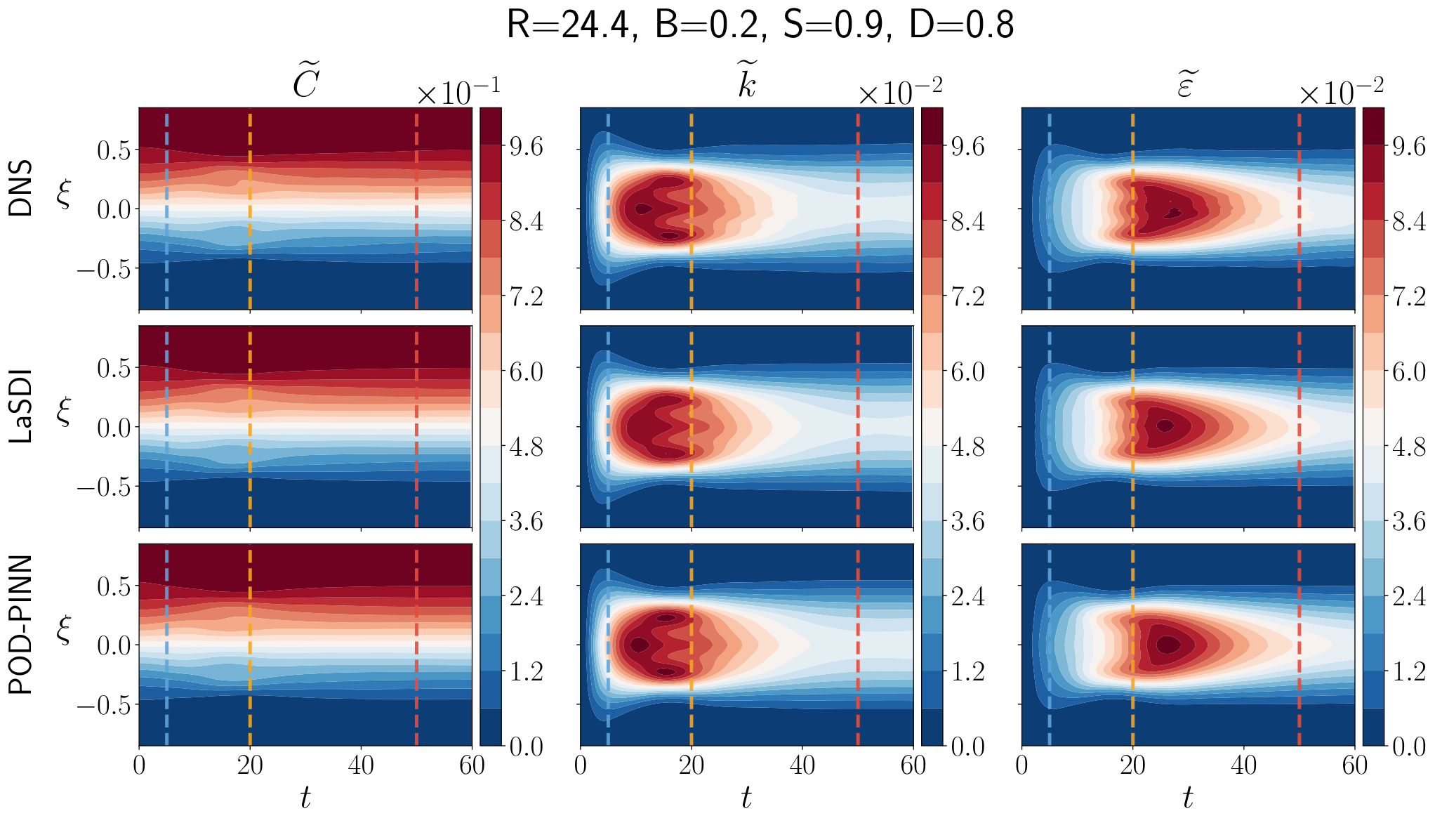
The space–time representations in Fig. 6 complement the instantaneous comparisons of Fig. 5 by showing how the profile shapes develop throughout the transition to turbulence. For this trajectory, the DNS fields exhibit pronounced spatial structures during the transient regime, including secondary lobes in the self-similar turbulent kinetic energy and dissipation profiles around . Both reduced-order models reproduce the location, persistence, and subsequent attenuation of these structures. The agreement demonstrates that LaSDI and POD-PINN capture not only the global growth of the instability but also the nontrivial spatial dynamics associated with the transition.
Such complex transient profiles are observed in particular for trajectories characterized by and . These parameters correspond to an initial interface perturbation dominated by relatively low wavenumbers and having a small initial amplitude, respectively, so that the interface is initially close to a flat configuration. Under these conditions, large coherent structures develop rapidly and accelerate away from the initial interface, accumulating kinetic energy. Their localized transport of kinetic energy and dissipation produces the secondary extrema, or bumps, visible in the one-dimensional profiles during the transition to turbulence regime. As the instability evolves, secondary Kelvin–Helmholtz-type instabilities develop along the shear layers surrounding these structures, promoting the generation of smaller scales and accelerating the transition toward turbulence (around ). This progressive cascade of spatial scales gradually smooths the profiles and leads to the parabolic self-similar shapes characteristic of the asymptotic regime.
The ability of both ROMs to recover these features is therefore an important result, since they arise from strongly transient and spatially localized dynamics rather than from the smoother late-time self-similar evolution.
5.2 Comparison across initial perturbations
Figure 7 compares the zero-dimensional predictions of the two reduced-order models for three representative simulations from the test set. The red trajectory corresponds to the inertial configuration considered in Figs. 5 and 6, the cyan trajectory represents an intermediate regime, and the purple trajectory corresponds to a diffusion-dominated configuration.
Additional comparisons between the surrogate models and the DNS are provided in Appendix B for trajectories with moderate or low initial Reynolds number , whose early-time evolution is primarily diffusion-dominated. This selection illustrates the good performance of the ROMs across markedly different transition dynamics.
Two dimensionless quantities are used to characterize the trajectories in the phase-space representation. The turbulent Froude number is defined here as
| (22) |
and compares the turbulent frequency, , with the characteristic stratification frequency, . The energy ratio
| (23) |
measures the fraction of the available potential energy converted into turbulent kinetic energy. Its derivation from the total-energy balance is detailed in Appendix C. This quantity is bounded by : the upper limit corresponds to a complete conversion of the available potential energy into turbulent kinetic energy in the absence of dissipation, whereas corresponds to the absence of kinetic-energy production from the available potential-energy reservoir.
Figure 7(a) shows that both models reproduce the main temporal trends of the integrated kinetic energy, dissipation, and mixing length for the three regimes. Their relative performance nevertheless depends on the initial condition and on the predicted quantity. These results indicate that neither reduced representation is uniformly superior across all dynamical regimes, especially for dissipation, which is particularly sensitive to the rapid development of small scales.
The trajectories in the phase space, shown in Fig. 7(b), provide a more compact view of the predicted dynamics. LaSDI has greater difficulty reproducing the initial part of the trajectories, where both dimensionless quantities vary rapidly. For the diffusion-dominated simulation, however, the LaSDI trajectory follows the DNS reference more closely in the phase-space than the POD-PINN prediction. In this phase space, the stable fixed point represents the self-similar state, in which both and are expected to become constant. The two ROMs preserve this attracting structure. However, the DNS trajectories do not extend sufficiently far into the self-similar regime to identify the reference fixed-point coordinates accurately. The differences between the limiting coordinates predicted by the two models should therefore be interpreted cautiously.
5.3 Test-set accuracy and physical consistency
Figure 8 compares the two reduced-order models only at times for which DNS reference data are available. The POD-PINN and LaSDI error distributions largely overlap for both the one-dimensional profiles and the associated zero-dimensional quantities, indicating comparable accuracy at the data-supported points. The mean errors are nearly identical for , , and , and remain of the same order for the other quantities. The larger errors in the earliest time interval mainly arise from predictions at , for which imperfect surrogate initialization is particularly pronounced in diffusion-dominated trajectories.
The modest differences depend on the predicted quantity rather than revealing a systematic advantage of either model. POD-PINN yields a lower mean error for the mixing length , whereas LaSDI is slightly more accurate for the dissipation profile and its integrated counterpart . The distributions generally broaden and shift toward larger errors with time, particularly for the turbulent quantities, but substantial overlap remains between the two models across the temporal intervals.
The latest distributions must nevertheless be interpreted with caution because the DNS trajectories do not all reach the same final time. The number of simulations contributing to each temporal bin therefore decreases with time, making the last intervals less statistically representative and more sensitive to individual trajectories. Moreover, because the errors are evaluated only where DNS data exist, this figure assesses interpolation and reconstruction accuracy rather than long-time extrapolation.
The zero-dimensional turbulent kinetic-energy balance (37) is imposed as a soft physical constraint during the training of both reduced-order models. Figure 9 therefore evaluates how well this constraint generalizes to unseen initial conditions and to times extending beyond the DNS data. Because its residual can be computed directly from the surrogate predictions without requiring a DNS reference, it provides a diagnostic of the internal consistency and physical coherence of the extrapolated quantities.
POD–PINN yields systematically smaller residuals than LaSDI over all temporal intervals, including the extrapolation regime. The mean absolute residual is for POD–PINN and for LaSDI, corresponding to a difference of approximately one order of magnitude. This separation indicates that the POD–PINN predictions remain more accurately coupled through the global kinetic-energy balance, even when evaluated beyond the data-supported time interval, suggesting more robust extrapolation capabilities.
The residuals of both models remain bounded and exhibit no systematic late-time drift, showing that neither ROM loses the constrained energy-balance structure during extrapolation. LaSDI thus retains qualitative consistency with the equation, while POD–PINN satisfies it substantially more accurately and uniformly.
6 Conclusion
This work compares two physics-guided parametric ROMs for Rayleigh–Taylor mixing across the transition to turbulence and the self-similar regime. POD–PINN combines an interpretable linear spatial decomposition with nonlinear neural-network dynamics, whereas LaSDI constructs a nonlinear latent representation governed by a linear evolution law. Their comparison therefore isolates a central modeling trade-off: whether complexity should be carried by the reduced representation or by the dynamics evolving within it.
For the POD–PINN approach, the separation between spatial modes and temporal amplitudes preserves one of the main advantages of classical modal decompositions. The leading POD modes can be directly associated with the global evolution and self-similar structure of the profiles, whereas the secondary modes describe the transient corrections associated with the development of coherent structures and the transition to turbulence. Symmetry, realizability, and self-similar scaling are introduced directly into the construction of the reduced representation, providing physically meaningful coordinates and facilitating the interpretation of the reconstructed fields. This spatial interpretability is obtained at the cost of a less interpretable temporal model. Unlike a classical POD–Galerkin formulation, the evolution of the modal amplitudes is not governed by an explicit low-dimensional system whose individual interaction terms can be analyzed directly, but by a neural network. The resulting closure is therefore implicit.
In contrast to the static solution map approach of POD-PINN, the second approach adopts a dynamical evolution model. Next, motivated by the observation that the temporal extent of observed trajectories in spatially extended dynamical systems is typically much too short, the second approach focuses simultaneously on keeping the latent space dimension very low and the dynamics simple. Limiting dynamics to be linear then requires the coordinate transformation step to be nonlinear to be able to limit the latent space dimension to be very low. The present results show that a latent dimension of only 4 (with minor degradation in performance at 2) is sufficient to obtain an efficient representation of the considered profiles while retaining linear latent dynamics. To reiterate, we find it surprising that strongly nonlinear and transient regimes can be reasonably well represented by linear dynamics in a very low dimensional latent space. Although the latent coordinates do not admit the direct physical interpretation of POD modes, the linear evolution law offers another route toward interpretability. In particular, classical dynamical-systems tools can be applied to the identified latent operator. The analysis of its eigenvalues and eigenvectors could reveal characteristic time scales, stability properties, bifurcation, dominant latent directions and the fixed points associated with the self-similar regime. Establishing explicit links between these latent structures and physical observables therefore constitutes a promising perspective.
Overall, the results demonstrate that the choice between linear and nonlinear reduced representations should not be based solely on reconstruction accuracy. POD–PINN is particularly suitable when physically identifiable spatial structures and explicit control over conservation properties are required. LaSDI is especially attractive when strong a priori assumptions about the relevant physics are unavailable: beyond providing a compact representation and efficient long-time integration, its learned latent structure and linear dynamics can serve as a data-driven discovery tool for formulating hypotheses about the underlying organization of the dynamics.
We experimented further with the second approach to see if prediction accuracy could be further improved by allowing for nonlinearity in the dynamics. This seemed to suggest that obtaining significant improvements over comparable accuracy of the two approaches presented may not be possible. As such, we speculate that nonlinearity in one of the two steps—coordinate transformation and latent-space dynamics/solution map—may be sufficient. This reinforces and reiterates our view that the two approaches are complementary rather than competing. Future work could combine their respective strengths, for example by introducing explicit physical observables into the LaSDI latent space, analyzing the spectrum of its latent dynamics matrix, or replacing the black-box temporal component of POD–PINN with a partially interpretable learned dynamical system. Such developments would contribute to reduced-order models that are simultaneously compact, predictive, physically consistent, and informative for the analysis and modeling of turbulent Rayleigh–Taylor mixing.
Appendix A Linear encoding-decoding based surrogate
A.1 POD details
This appendix provides additional details on the POD representation introduced in Section 3. It first establishes the relation between the modal amplitudes and the zero-dimensional quantities, then clarifies the connection between the leading POD modes and the self-similar profiles, and finally separates the error associated with the truncated spatial basis from that introduced by the PINN prediction of the modal amplitudes.

A.1.1 Zero-dimensional quantities
The zero-dimensional quantities defined in Eq. (9) can be evaluated directly from the reduced coordinates, without reconstructing the profiles on the spatial grid.
| (24) |
For the positive quantities represented through their square roots, orthonormality eliminates the cross terms in the spatial integral. The spatial moment of the th mass-flux mode is defined as
| (25) |
where . This interval is wider than the nominal mixing-layer region because the turbulent profiles develop diffuse tails that extend beyond its boundaries. Retaining these tails improves the accuracy of both the modal representation and the spatially integrated quantities.
Figure 10 presents the first five modes obtained after applying the symmetry and realizability transformations described in Section 3. The leading modes are smooth and reproduce the dominant spatial support of the mixing layer. The secondary modes contain an increasing number of extrema and progressively finer spatial scales, consistently with their role in representing transient profile deformations. Five modes are retained for all quantities except the mean concentration, for which the first four modes are sufficient; its fifth mode is nevertheless displayed for comparison.


A.1.2 Asymptotic interpretation of the leading POD modes
Because the POD is performed directly on the self-similar quantities, higher-order amplitudes decay toward zero. The leading amplitude approaches a constant, , and the asymptotic profile is governed by the first mode. For all non-negative quantities represented through their square roots,
| (26) |
For the mean concentration and the modeled negative mass flux, which are decomposed without the square-root transformation, the relation remains linear:
| (27) |
The leading POD mode is therefore directly proportional to the asymptotic self-similar profile for and , and to its square root for the positive quantities.
A.2 PINN implementation details
This appendix complements the POD–PINN presentation in Sec. 3 by collecting the implementation details omitted from the main text. It describes the input and output preprocessing, the complete loss function, the construction of the physical residuals, the collocation-point strategy, and the reconstruction-error assessment.
A.2.1 Preprocessing and output parametrization
For both POD–PINN and LaSDI, only the first of the temporal samples from each training trajectory are used for model fitting, while the final are withheld to assess temporal-extrapolation capabilities, as illustrated in Fig. 11.
The four initial-condition parameters are logarithmically transformed, while the dimensionless time is left unchanged:
| (28) |
All outputs, including , are subsequently normalized to . A squared Softplus transformation is applied to the output to promote its expected quadratic late-time growth, see Eq.(10). Softplus activations are also used in the hidden layers because their smoothness facilitates derivative evaluation by automatic differentiation.
A.2.2 Data-driven loss function
Terms of the loss function are constructed from mean-squared-error (MSE). For two tensors and of identical shape, the MSE is defined as
| (29) |
where is the total number of elements in each tensor and indexes their flattened entries. The data-driven loss is then written as the weighted sum of four contributions:
| (30) |
The initial value is penalized separately to prevent it from being underweighted relative to the remaining time samples:
| (31) |
| (32) |
The expansion-rate term compares the derivative obtained by automatic differentiation with the DNS reference:
| (33) |
The modal term uniformly weights the rescaled POD amplitudes; energy-based weighting was also tested but did not improve the prediction accuracy:
| (34) |
Figure 12 shows that the learned errors follow the modal hierarchy, with the leading modes predicted most accurately.

A.2.3 Physics-informed loss function
The physics-informed contribution used during training is
| (35) |
Negative predicted values of are penalized by
| (36) |
The spatially integrated balance of kinetic energy is
| (37) |
Substitution of the retained POD expansions (24), gives
| (38) |
where is the spatial integral of mode and repeated indices are summed. The truncation residual is denoted for DNS-projected amplitudes and for PINN predictions. Only the latter is minimized:
| (39) |
This formulation lets the learned retained-mode dynamics accounts implicitly for unresolved contributions, without fitting the DNS residual outside the available sampling points.
The governing advection–diffusion equation is
| (40) |
In the self-similar formulation,
| (41) |
Substitution of the retained POD expansions yields
| (42) |
where the explicit dependence on is omitted. The corresponding loss is
| (43) |
Because explicitly involves the POD modes and their spatial derivatives, this term constrains both the modal dynamics and the reconstructed profile shapes while providing an implicit closure for discarded modes.
A.2.4 Collocation points and residual-based attention
The physical residuals are evaluated at collocation points, which require no reference DNS values and can therefore extend beyond the available trajectories. To provide extrapolation constraints without sampling unphysical configurations, these points are generated by Latin Hypercube Sampling (Stein, 1987) within
| (44) |
This domain covers both the DNS database and neighboring unexplored regions. During training, Residual-Based Attention (Anagnostopoulos et al., 2024) adaptively increases the weight of points with large physical residuals, thereby concentrating the optimization on the most difficult temporal and parametric regimes.
A.2.5 Reconstruction accuracy
Finally, Fig. 13 separates the error caused by POD truncation from that introduced by the learned temporal dynamics. The POD–DNS reconstruction uses amplitudes obtained by projecting the DNS profiles onto the truncated basis and therefore isolates the spatial-representation error. The POD–PINN reconstruction instead uses the predicted amplitudes, so that the difference between the two distributions measures the additional error introduced by the neural network.
The direct POD reconstruction provides the lower-error baseline for all quantities, as expected, while the POD–PINN distributions follow the same temporal trends with an additional contribution from the predicted amplitudes. The errors generally increase and broaden with time, but the mean POD–PINN error over the complete test set remains between approximately and , depending on the quantity. The concentration profile is reconstructed most accurately, whereas the square-root-transformed turbulent quantities are more sensitive to errors in the predicted amplitudes after transformation back to physical space. Overall, the selected basis remains sufficiently compact to preserve physical interpretability while providing an accurate representation for the surrogate model.
Appendix B Additional ROM comparisons
In this section, we provide two additional comparisons between the DNS and surrogate-model predictions for representative test cases shown in the phase diagram of Fig. 7. For the diffusion-dominated trajectory with initial Reynolds number , selected one-dimensional profiles of the mean concentration , kinetic energy , and dissipation are presented in Fig. 14. The corresponding space–time evolution is shown in Fig. 15.
Appendix C Total Energy conservation
Under the Boussinesq approximation, the dimensionless density field, normalized by the average of the pure-fluid densities, is related to the heavy-fluid concentration field by
| (45) |
Assuming that the mean concentration profile is piecewise linear, the variation in potential energy relative to the initial condition, , can then be estimated as (Cook et al., 2004)
| (46) |
where denotes the fluid volume (again quantities are non dimensionalized). Thus, the magnitude of the potential energy released into the system increases as the mixing layer grows.
References
- Residual-based attention in physics-informed neural networks. Computer Methods in Applied Mechanics and Engineering 421, pp. 116805. External Links: ISSN 0045-7825, Document, Link Cited by: §A.2.4, §3.3.
- A simple experiment to investigate two‐dimensional mixing by rayleigh–taylor instability. Physics of Fluids A: Fluid Dynamics 2 (6), pp. 922–927. External Links: ISSN 0899-8213, Document, Link, https://pubs.aip.org/aip/pof/article-pdf/2/6/922/12772845/922_1_online.pdf Cited by: §2.3.
- The proper orthogonal decomposition in the analysis of turbulent flows. Annual Review of Fluid Mechanics 25, pp. 539–575. External Links: Document, Link Cited by: §1.
- Inertial-confinement fusion with lasers. Nature Physics 12 (5), pp. 435–448 (en). External Links: ISSN 1745-2481, Link, Document Cited by: §1.
- A comprehensive review of latent space dynamics identification algorithms for intrusive and non-intrusive reduced-order-modeling. External Links: 2403.10748, Link Cited by: §1, §1.
- Autoencoders reloaded. Biological Cybernetics 116 (4), pp. 389–406. External Links: Document, Link, ISSN 1432-0770 Cited by: §1.
- Auto-association by multilayer perceptrons and singular value decomposition. Biological Cybernetics 59 (4), pp. 291–294. External Links: Document, Link, ISSN 1432-0770 Cited by: §1.
- Polynomial autoencoders with quantifiable errors for nonlinear fluid flow reconstruction. Research Square. Note: Preprint External Links: Document, Link Cited by: §1.
- AutoEncoders latent space interpretability in the light of proper orthogonal decomposition: machine learning of periodically forced fluid flows. Computer Physics Communications 315, pp. 109728. External Links: ISSN 0010-4655, Document, Link Cited by: §1.
- The turbulent Faraday instability in miscible fluids. Journal of Fluid Mechanics 883, pp. A57. External Links: Document Cited by: §2.
- Poisson solvers for strongly stratified turbulent flows. Computers & Fluids, pp. 106741. Cited by: §2.
- Quasi-self-similarity of the horizontal magnetic rayleigh–taylor instability. Journal of Fluid Mechanics 1023, pp. A20. Cited by: §2.
- Machine learning for fluid mechanics. Annual Review of Fluid Mechanics 52 (Volume 52, 2020), pp. 477–508. External Links: Document, Link, ISSN 1545-4479 Cited by: §1.
- Multiscale model reduction for incompressible flows. Journal of Fluid Mechanics 973, pp. A3. External Links: Document Cited by: §1.
- Data-driven discovery of coordinates and governing equations. Proceedings of the National Academy of Sciences 116 (45), pp. 22445–22451. External Links: Document, Link, https://www.pnas.org/doi/pdf/10.1073/pnas.1906995116 Cited by: §1, §1.
- The mixing transition in rayleigh–taylor instability. Journal of Fluid Mechanics 511, pp. 333–362. External Links: Document Cited by: Appendix C.
- Learning turbulence closures with physics-informed neural networks for the rayleigh-taylor transition to turbulence. External Links: 2607.07020, Link Cited by: §1.
- Low‐dimensional models for complex geometry flows: application to grooved channels and circular cylinders. Physics of Fluids A: Fluid Dynamics 3 (10), pp. 2337–2354. External Links: ISSN 0899-8213, Document, Link, https://pubs.aip.org/aip/pof/article-pdf/3/10/2337/12601781/2337_1_online.pdf Cited by: §1.
- The approximation of one matrix by another of lower rank. Psychometrika 1 (3), pp. 211–218. External Links: Document, Link Cited by: §3.1.
- On latent dynamics learning in nonlinear reduced order modeling. Neural Networks 185, pp. 107146. Cited by: §1, §1.
- Frozen waves in turbulent mixing layers. Phys. Rev. Fluids 4, pp. 064608. External Links: Document, Link Cited by: §2.
- Efficient nonlinear manifold reduced order model. External Links: 2011.07727, Link Cited by: §1.
- Dynamical systems of continuous spectra. Proceedings of the National Academy of Sciences 18 (3), pp. 255–263. External Links: Document, Link, https://www.pnas.org/doi/pdf/10.1073/pnas.18.3.255 Cited by: §1.
- Hamiltonian systems and transformation in hilbert space. Proceedings of the National Academy of Sciences 17 (5), pp. 315–318. External Links: Document, Link, https://www.pnas.org/doi/pdf/10.1073/pnas.17.5.315 Cited by: §1.
- Hybrid autoencoder/galerkin approach for nonlinear reduced order modelling. Computers & Fluids 302, pp. 106811. External Links: ISSN 0045-7930, Document, Link Cited by: §1.
- Development of the indirect-drive approach to inertial confinement fusion and the target physics basis for ignition and gain. Physics of Plasmas 2 (11), pp. 3933–4024 (en). External Links: ISSN 1070-664X, 1089-7674, Link, Document Cited by: §1.
- Deep learning for universal linear embeddings of nonlinear dynamics. Nature Communications 9 (1), pp. 4950. External Links: Document, Link, ISSN 2041-1723 Cited by: §1.
- A low-dimensional model for simulating three-dimensional cylinder flow. Journal of Fluid Mechanics 458, pp. 181–190. External Links: Document Cited by: §1.
- CD-rom: complemented deep - reduced order model. Computer Methods in Applied Mechanics and Engineering 410, pp. 115985. External Links: ISSN 0045-7825, Document, Link Cited by: §1.
- Revealing low-dimensional structure in 2d richtmyer-meshkov instabilities via parametric reduced-order modeling. External Links: 2510.16197, Link Cited by: §1.
- Reduced-order modelling for flow control. Springer. Cited by: §1.
- A hierarchy of low-dimensional models for the transient and post-transient cylinder wake. Journal of Fluid Mechanics 497, pp. 335–363. External Links: Document Cited by: §1.
- PyTorch: an imperative style, high-performance deep learning library. External Links: 1912.01703, Link Cited by: §3.3.
- Physics-informed neural networks: a deep learning framework for solving forward and inverse problems involving nonlinear partial differential equations. Journal of Computational Physics 378, pp. 686–707. External Links: ISSN 0021-9991, Document, Link Cited by: §1, §3.3.
- Investigation of the character of the equilibrium of an incompressible heavy fluid of variable density. Proceedings of the London Mathematical Society 6 (2), pp. 170–177. External Links: Document Cited by: §1.
- Rayleigh–Taylor instabilities in high-energy density settings on the National Ignition Facility. Proceedings of the National Academy of Sciences 116 (37), pp. 18233–18238 (en). External Links: ISSN 0027-8424, 1091-6490, Link, Document Cited by: §1.
- Rayleigh–taylor turbulence: self-similar analysis and direct numerical simulations. Journal of Fluid Mechanics 507, pp. 213–253. External Links: Document Cited by: §2.5.2.
- Reconstruction equations and the karhunen–loève expansion for systems with symmetry. Physica D: Nonlinear Phenomena 142 (1), pp. 1–19. External Links: ISSN 0167-2789, Document, Link Cited by: §1.
- An overview of Rayleigh-Taylor instability. Physica D: Nonlinear Phenomena 12 (1), pp. 3–18. External Links: ISSN 0167-2789, Link, Document Cited by: §2.5.
- Turbulence and the dynamics of coherent structures part i: coherent structures. Quarterly of Applied Mathematics 45 (3), pp. 561–571. External Links: Link Cited by: §1, §3.1.
- Large sample properties of simulations using latin hypercube sampling. Technometrics 29 (2), pp. 143 – 151. Note: Cited by: 2163 External Links: Document, Link Cited by: §A.2.4.
- Modal analysis of fluid flows: an overview. AIAA Journal 55 (12), pp. 4013–4041. External Links: Document, Link, https://doi.org/10.2514/1.J056060 Cited by: §1.
- The instability of liquid surfaces when accelerated in a direction perpendicular to their planes. i. Proceedings of the Royal Society of London. Series A, pp. 192–196. Cited by: §1.
- Database of direct numerical simulations of rayleigh–taylor turbulence at low density contrast: 0d volume-averaged quantities. Recherche Data Gouv. External Links: Document, Link Cited by: §2.2.
- Leveraging initial conditions memory for modelling rayleigh–taylor turbulence. Journal of Fluid Mechanics 1009, pp. A17. External Links: Document, Link Cited by: §1, §2.2, §2.
- Modeling late-time sensitivity to initial conditions in boussinesq rayleigh–taylor turbulence. Physica D: Nonlinear Phenomena 483, pp. 134947. External Links: ISSN 0167-2789, Document, Link Cited by: §2.5.2, §2.5, §2.
- Unveiling the optimization process of physics-informed neural networks: how accurate and competitive can pinns be?. Journal of Computational Physics 523, pp. 113656. External Links: Document, Link Cited by: §3.3.
- Decoding complexity through machine learning is redefining scientific discovery. Communications Physics 9 (1), pp. 168. External Links: Document, Link, ISSN 2399-3650 Cited by: §1.
- A pinn methodology for temperature field reconstruction in the piv measurement plane: case of rayleigh–bénard convection. International Communications in Heat and Mass Transfer 167, pp. 109284. External Links: ISSN 0735-1933, Document, Link Cited by: §1.
- Numerical simulation of turbulent mixing by rayleigh–taylor instability. Physica D: Nonlinear Phenomena 12 (1), pp. 32–44. External Links: Document, Link Cited by: §2.5.2.
- Instabilities and Mixing in Inertial Confinement Fusion. Annual Review of Fluid Mechanics 57 (1), pp. 197–225 (en). External Links: ISSN 0066-4189, 1545-4479, Link, Document Cited by: §1.
- Rayleigh–taylor and richtmyer–meshkov instability induced flow, turbulence, and mixing. i. Physics Reports 720-722, pp. 1–136. Note: Rayleigh–Taylor and Richtmyer–Meshkov instability induced flow, turbulence, and mixing. I External Links: ISSN 0370-1573, Document, Link Cited by: §1.
- Rayleigh–taylor and richtmyer–meshkov instability induced flow, turbulence, and mixing. ii. Physics Reports 723-725, pp. 1–160. Note: Rayleigh–Taylor and Richtmyer–Meshkov instability induced flow, turbulence, and mixing. II External Links: ISSN 0370-1573, Document, Link Cited by: §1.