Wing-Rotor Aerodynamic Interactions in Small UAVs During Hover and Cruise
Dev Pradeepkumar Nayak1, Seungmin Choi1,2, and Muhammad Saif Ullah Khalid1,∗
1Nature-Inspired Engineering Research Lab (NIERL), Department of Mechanical and Mechatronics Engineering, Lakehead University, Thunder Bay, ON P7B 5E1, Canada
2Department of Unmanned Aircraft Systems, Hanseo University, Seosan, Republic of Korea
∗Corresponding Author, Email: mkhalid7@lakeheadu.ca
Abstract
A compact vertical take-off and landing aircraft requires the same tilt-rotor configuration to perform two fundamentally different aerodynamic tasks: sustain hover and deliver efficient cruise. This work investigates the underlying wing-rotor interactions in both operating regimes using a validated unsteady Reynolds-averaged Navier-Stokes equations-based computational framework. For cruise, the advance ratio governs the balance between thrust production, propulsive efficiency, and wake coherence. Lower advance ratios produce a tightly wound slipstream that undergoes strong vortex interactions, leapfrogging, and early wake bifurcation. At higher advance ratios, the slipstream retains a narrower and more coherent jet-like structure, improving propulsive efficiency while reducing both thrust of the propellor and lift of the wing. The flow impingement at the wing is characterized through the approaching, interaction, and convection phases, revealing the combined influence of vortex stretching, wake bifurcation, blockage, image-induced velocity, and streamwise momentum convection on the downstream wake. In hover, the propeller’s rotational speed governs the overall aerodynamic performance more strongly than the wing’s placement. Although the position of the wing with respect to the propellor modifies the local wake interactions and flow impingement on its leading edge, its influence on the integrated thrust coefficient and figure of merit remains limited. We also explain the vortex and wake dynamics around the propellor and the wing responsible for governing these aerodynamic performance.
1 INTRODUCTION
Recent advancements in drone technology facilitates their application across a broad spectrum of fields, ranging from recreational activities and high-end cinematography to sophisticated military operations [1]. These developments are driven by substantial progress in engineering methodologies, particularly in the advancement of reliable computational and experimental fluid dynamics frameworks [2]. Broadly, presently existing unmanned aerial vehicles (UAVs) can be categorized into two primary classes, including fixed-wing UAVs and multi-rotor UAVs. Fixed-wing UAVs resemble scaled-down aircraft, generating lift through forward motion, whereas multi-rotor UAVs operate similarly to helicopters, producing lift directly through rotating propellers, enabling vertical takeoff and hovering capabilities [1, 3, 4, 2].
Both categories offer distinct advantages while also exhibiting some inherent limitations too. To overcome these constraints, a third class of UAVs emerged, commonly referred to as vertical take-off and landing (VTOL) aircraft [3, 5]. These configurations combine the capabilities of multi-rotor and fixed-wing aircraft, enabling vertical takeoff and landing through a rotor-supported flight mode, followed by a transition to forward flight through tilting rotors. Therefore, their operation can be broadly divided into three primary flight states: (i) cruise, corresponding to forward flight, and (ii) hover, relating to holding a station aerially, and (iii) vertical takeoff and landing. Although the applications and parametric scaling of such UAVs were extensively investigated, studies focusing on smaller-scale configurations, specifically making it relevant to low Reynolds numbers remained comparatively limited. UAVs classified as “mini” are generally characterized by a representative dimension related to the propellor with a diameter of less than for its blades [1]. Accordingly, the configuration considered in our present investigation may be classified as a mini-UAV, with a propeller’s diameter of .
Owing to the close proximity of the wing and propeller VTOL aerial vehicles, it is crucial to investigate the design and operating parameters that govern the aerodynamic performance of the UAV at different cruising speeds and during hover or takeoff/landing. Within the complex framework of a VTOL UAV transitioning between hover and cruise, design or operating parameters that improve performance in one flight regime may have a detrimental effect in the other, and vice versa. Therefore, both the design parameters and operating parameters must be selected with consideration of their coupled effects, such that an appropriate balance is achieved between the overall hover and cruise performance of the VTOL UAV.
For the VTOL UAV operating under cruise conditions, the placement of the wing near the propeller wake can be considered analogous to the configuration investigated by Muscari et al. [6]. Although their study focused on a marine propeller, the underlying principles governing the flow field, wake development, and vortex interactions between the propeller blades and the wing remain relevant to the presently considered configuration. Previous studies examining wing–rotor interactions in forward flight primarily considered the advance ratio, cruising velocity, and relative placement of the wings as the major operating and design parameters [7, 8, 9, 10, 6]. Accordingly, the primary objective of the present study under cruising conditions is to identify the combination of these parameters that yields the highest propulsive efficiency. The resulting quantitative trends are further interpreted through the analysis of vortex–body and vortex–vortex interactions. Under cruise conditions, the wing’s position is fixed at a distance of from the nacelle and from the propeller-blade centreline. These specifications come from the configuration investigated by Zawodny et al. [3]. Their study examined the influence of the wing’s placement and demonstrated that positioning the wing closer to both the propeller and the nacelle resulted in higher thrust generation. This finding provides the primary justification for maintaining the position of the wing unchanged throughout our simulations related to cruise flight.
For the cruise conditions considered in our current work, classical scaling-related arguments indicate that, to maintain levels of thrust comparable to those of larger-scale propellers, a small-scale propeller must operate at a higher rotational speed, which consequently alters the resulting wake structure [7]. Based on the operating ranges commonly reported in the literature, the propeller is expected to perform well over a broad range of advance ratios (), and at cruising speeds () of up to [7, 8, 9]. Here, we define the advance ratio as , where denotes the angular frequency of the propellor, and is diameter of the propellor.
Under hovering conditions, the absence of a freestream requires the propeller to generate enough momentum needed to support the vehicle, which makes induced power a dominant aerodynamic requirement [11, 12]. The resulting wake gets contracted downstream and contains concentrated helical tip vortices whose trajectory, circulation, and core development strongly influence the induced velocity, thrust, torque, and loading on the blade [13, 14]. When a wing is located within this wake, vortex impingement and accelerated downwash can produce non-uniform loading and reduce the net vertical force available to the aircraft [15, 16]. These effects depend mainly on the propeller’s speed and relative placement of the wing, making it an important aspect of operating VTOL UAVs and one of the main research objectives of our present study.
With this context and background, we particularly focus on addressing the following important yet unanswered research questions: (i) how does the propeller-wing interactions affect the aerodynamic performance across the range of conventional advance ratios in cruise? (ii) how does the positioning of the wing affect the performance of the propeller over a wide range of operating angular speeds in hover? and (iii) how does the presence of the wing influence the evolution of the propeller’s slipstream in both cruise and hover? Addressing these aspects is important to analyze the performance of a tilting rotor configuration under both cruise and hover conditions to optimize its overall aerodynamic capabilities in VTOL UAVs. To define a more focused yet representative parametric space, the present investigation considers freestream velocities of , , and , with the advance ratio ranging from of propellors for the investigations of propellor-wing interactions during cruise conditions. Nevertheless, there is no freestream aerial flow for hover-related conditions. Here, we consider a broad range of rotational speeds of the propellor, comprising , , , and . We also consider specific locations for placement of the wing with respect to the propellor, as shown in Fig. 6.
2 COMPUTATIONAL METHODOLOGY
In this research work, we consider the Gemfan propeller, which is commonly used in first-person view () drones [17]. The present work focuses on analyzing the operation of a VTOL configuration at high angular velocities. Although airfoils, such as NACA can be effective for lift generation, they typically exhibit higher drag coefficients [18]. Contrarily, more streamlined symmetric airfoils produce a uniform pressure distribution between the upper and lower surfaces, and may not generate sufficient lift [18]. Here, we select NACA airfoil for the wing’s profile. This airfoil offers a favorable balance between thickness and camber, enabling the generation of sufficient pressure difference for lift production while maintaining relatively low drag. The main geometrical features of the propeller are reported in Table. 1.
| Gemfan 51466 FPV model | |
| Radius | |
| Number of blades | |
| Pitch ratio | |
| Hub ratio | |
The VTOL configuration is illustrated in Fig. 1, along with the non-dimensional propeller radius and wing chord length. The schematics presented in Figs. 1a and 1b represent the orientations of the propeller-wing configuration with respect to an aircraft (outlined in blue) in cruise and hover, respectively. Please note that this outline of an airplane is included solely to indicate the orientation of the VTOL flight and is not part of the currently reported simulations.). The normalized locations of the wing relative to the centerline of the propellor and nacelle are shown in the enlarged views in Figs. 1c and 1e for the cruise and hover configurations, respectively. Figure 1d shows an isometric view of the VTOL configuration and identifies the components considered in this work. In Figs. 1c and 1e, and represent the axial and vertical locations of the wing leading edge relative to the propeller centerline and nacelle, respectively.

We perform our computational simulations in OpenFOAM-v2412 by solving unsteady Reynolds-averaged Navier-Stokes (URANS) equations, employing Shear Stress Transport (SST) turbulence model [19]. This hybrid model combines the near-wall accuracy of the – model and the free-stream robustness of the model [20, 21]. The SST model incorporates a shear stress limiter to improve predictions under adverse pressure gradients and flow separation. The non-dimensional continuity and incompressible URANS turbulence equations are given below [19, 21, 20, 22].
| (1) |
| (2) |
Where is the pressure, and the last term, , corresponds to the Reynolds stress tensor, which accounts for the transport of momentum induced by turbulent velocity fluctuations. For closure of the governing set of equations, Reynolds stresses are modeled using the Boussinesq eddy-viscosity approximation, relating them to the mean strain rate through an eddy viscosity. In Eqs. 1 and 2, denotes the normalized mean velocity vector, is the normalized pressure, and Re is the Reynolds number for characterizing the flow. The temporal term is discretized using an implicit backward difference scheme. This algorithm combines the Pressure-Implicit with Splitting of Operators () algorithm and Semi-Implicit Method for Pressure-Linked Equations () algorithm. The convergence criterion for the iterative solution at each time step is set to [23].

Figure 2 shows the unstructured grid used for our simulations. The domain in Fig. 2a and 2c is normalized using the radius of the propeller. In order to handle the rotational motion of the propeller, a sliding mesh technique is used. The mesh is segregated in two regions, including a static zone that belongs to the part of the main domain, in which the rotating zone of the mesh is enclosed, as shown in Fig. 2b for cruise and Fig. 2d for hover. The rotating zone encloses the hub and the propeller blades and has a radius of . The interpolation of numerics between the static and the rotating zone is handled using a cyclic AMI-type boundary condition, and the tolerance is set to [23].

In Fig. 3, the grid refinement around the geometry is shown from sectional and frontal views. The near-wall regions are resolved with a maximum value of approximately , corresponding to the buffer layer of wall-bounded turbulent flow. This region lies between the viscous sublayer and the logarithmic layer, where neither a fully wall-resolved nor a conventional wall-function treatment is strictly applicable. However, these intermediate values are retained in our URANS simulations employing the SST model to balance computational cost and near-wall resolution. Around the curved surfaces, the value decreases further toward . The refined grids around the propeller, nacelle, and wing are shown in Figs. 3a, 3b, and 3c, respectively. Figures 3a and 3b also exhibit directions of the inlet flow for the cruise and hover configurations. As stated previously, for the hovering configurations.
2.1 Verification & validation
The grid is resolved enough to ensure the validity of the SST model. To further justify resolution of the grid and confidence in in our meshing approach, the grid-convergence tests are performed by choosing three grid resolutions. For the grid-convergence and time-step independence tests, we perform the simulations for total revolutions, with and . The simulations attain steady state solutions within revolutions. The three grids chosen for the grid-convergence study are: Grid 01 with 19,315,706 () cells, Grid 02 with 39,772,704 () cells, and Grid 03 with 51,544,856 () cells. Figure 4 shows the wing-tip vortex and the bound vortex generated around the wing, along with the tip vortices shed from the blades of the propeller. Upon closer inspection of the highlighted region of a blade of the propellor in Figs. 4a–4c, we observed that an increasing refinement of, of the grid helps capture the vortex formation and detachment from the surface of the blades. With finer grids, the near-blade vortical structures appear more coherent and resolved, which indicates improved resolution of the local flow physics from the model. However, despite these differences near the blade surface, the downstream vortices generally maintain a consistent shape and trajectory across all grid levels. It suggests that the wake features are relatively insensitive to further grid refinement and the accuracy of the model. Furthermore, we also conduct the time-step independence analysis using , , and time steps per revolution of the propellor. To further quantify the results of the grid-convergence and timestep-independence studies, the relative error () between different grids and time step sizes is defined using the following expression:
| (3) |
where denotes the reference case against which case is compared, and represents the parameter under consideration. In the present study, case corresponds to Grid 03, while case corresponds to Grid 01 and Grid 02. The parameter represents the mean thrust coefficient (). The relative errors obtained from both the grid-independence and time-step independence analyses are summarized in Table 2. These results indicate that the error between obtained from Grid 01 and Grid 03 is comparable to that from Grid 02 and Grid 03. Similarly, the variation in error across , , and time-steps per rotational cycle remains negligible. Therefore, we employ Grid 01 for our actual simulations related to this work while using time-steps in one revolution of the propellor.

| Grids (%) | Time-step (%) | |||
| Quantity | 01 & 03 | 02 & 03 | 1800 & 2600 | 2000 & 2600 |
| 4.01 | 3.40 | 0.10 | 0.03 | |
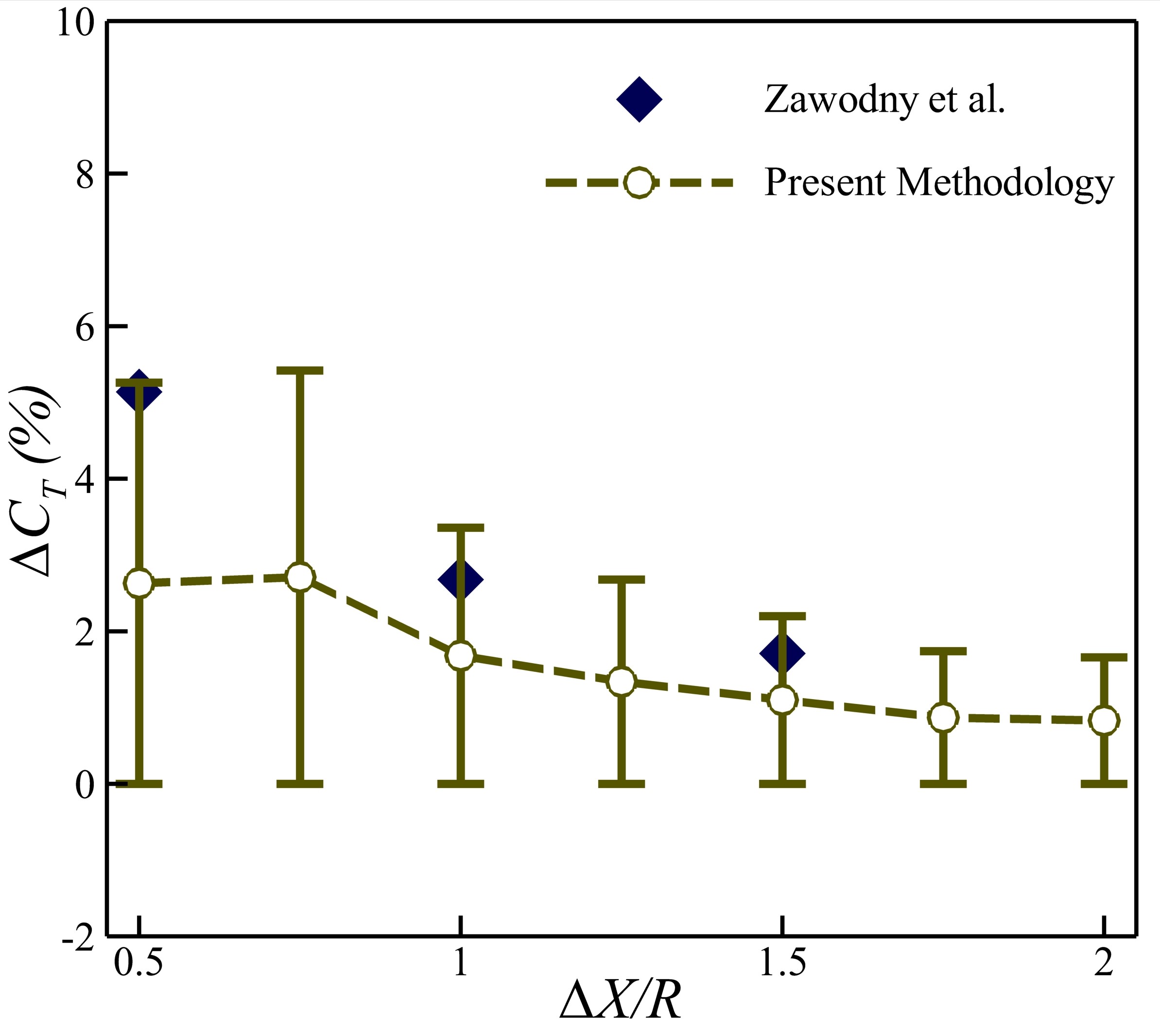
Next, we validate robustness and accuracy of our computational framework and the used turbulence model by comparing our results with those from Zawodny et al. [3]. Their work investigates a VTOL configuration with propeller–wing interaction in the near wake, examining the effect of wing’s location relative to centerline of the nacelle () and the axis of the propeller (). Following the experiments from Zawodny et al. [3], we carry out our simulations using an advance ratio of with an angular velocity of of the propellor for configurations with and without the wing. For the cases with the wing, it is placed at different locations (). How the wing’s position influences the aerodynamic performance of the propellor is quantified using the percentage difference in thrust coefficients, , obtained from configurations with and without the wing. Figure 5 presents as a function of based on their reported experimental data. The results indicate that increasing reduces the difference in thrust coefficient, as the influence of the wing on the propeller’s wake diminishes. Figure 5 shows that the present methodology captures the overall decreasing trend of with increasing , demonstrating a good agreement between our results and those from the experimental data reported by Zawodny et al. [3]. Minor deviations might be caused because they utilized a Mejzlik three-bladed carbon fiber propeller and a MOD B airfoil-based wing, which differs from the configuration employed in the present study. Additionally, radius of the propeller in their work is reported as , whereas we employ in the present work. It is important to mention that the aerodynamic performance metrics can be compared here based on similarity (affinity) laws, which corresponds to maintaining the same advance ratio [24, 25].
3 RESULTS & DISCUSSION
To facilitate navigation through the findings of our investigations, we divide this section in two subsections. Section 3.1 focuses on the analysis and results of the propeller-wing configuration in cruise, whereas Section 3.2 focuses on the same configuration in hover. Although the two subsections form a continuous analysis and discussion, this division provides a clear distinction between the two operating conditions.

In a VTOL aircraft, the placement of the wing within the near wake of the propeller is important, because the wing is the first downstream structural component to interact with the propeller slipstream. As discussed earlier, the experimental work by Zawodny et al. [3] quantified the effects of a wing’s placement at different axial and vertical locations relative to the propeller’s centerline and its axis of rotation. It motivates the present investigation of the propeller-wing interactions during cruise at different freestream velocities and advance ratios. Figure 6a shows location of the fixed wing used employed for our analysis for the cruising condition. For the hovering configuration, the analysis focuses on effects of the wing’s placement at different positions in the - and -directions, as shown in Fig. 6b, over a range of rotational speeds of the propellor.
3.1 Propeller-Wing Configuration in Cruise
For this part of our work, the vertical and axial wing positions are fixed at and , respectively. The freestream velocities are selected as , , and . Previous studies reported that increasing the advance ratio from to generally increased propulsive efficiency while reducing the thrust coefficient [2, 26, 5]. Accordingly, the advance ratio is varied from to in increments of . The operating parameters used in the analysis for cruising are listed in Table 3.
| Parameter | Symbol | Value |
| Freestream velocity () | , , | |
| Advance ratio | – | |
| Vertical wing position | ||
| Axial wing position |
Smaller and drones experience lower Reynolds number compared to their larger counterparts. The propellers with larger blade diameter often experience Reynolds number of over operating at [7, 27]. Based on the relationship between the angular velocity, freestream velocity and the advance ratio, the calculated RPM alongside their corresponding Reynolds number is shown in Fig. 7, which shows the operating of the propeller, ranging from to , based on the advance ratio required to maintain Re less than .

The efficiency of the propeller and the thrust coefficient versus are plotted in Fig. 8. These plots clearly exhibit the region of maximum efficiency and the corresponding thrust coefficient. The trend observed here follows the trend of optimal efficiency close to the advance ratio around , and these trends also show that the efficiency starts dropping with further increasing to .


Under the operating condition of , the present study reports operating efficiencies of , , and for the considered freestream velocities, corresponding to of , , and , respectively. These results also indicate that propellers of drones at this scale may operate at relatively high rotational speeds in the proposed configuration. Furthermore, the cambered wing considered here generates positive lift across all investigated advance ratios. Figure 9 presents the time-averaged lift coefficient () of the wing at different values of and . The lift coefficient exhibits a decreasing trend similar to that of the thrust coefficient shown in Fig. 8. However, the operating condition corresponding to the maximum propulsive efficiency does not necessarily produce the maximum lift by the wing. As discussed later, operation at higher advance ratios produces a narrower and more coherent jet-like propeller slipstream that retains its streamwise momentum farther downstream after impinging on the wing. The resulting localized flow acceleration beneath the wing reducing the pressure on the bottom-side surface, thereby decreasing the pressure difference across the wing and producing a corresponding reduction in the net .
At a given and diameter of the propellor, lower correspond to higher . A propeller operating at low generally associates with reduced due to increased blade loading, induced velocity, and energy losses within the slipstream. Now, we link link the aerodynamic performance metrics with unsteady flow dynamics around the propellor and the wing. Figures 10a and 10c present the propeller slipstream visualized using a -criterion isosurface of at a cruise velocity of with and , respectively. Figures 10b and 10d show the corresponding contours of the cycle-averaged streamwise velocity. At , the slipstream exhibits weak wake coherence, as shown in Fig. 10a. Successive tip vortices interact through an early-stage leapfrogging mechanism, highlighted by the yellow box. Because of the high here, successive tip vortices from blades of the propellor are generated at a rate greater than their downstream convection, resulting in a reduced helical pitch and closely spaced vortex filaments [28]. The reduced spacing promotes strong mutual induction between successive tip vortices, leading to vortex pairing, leapfrogging, and roll-up [9, 29]. These interactions may subsequently produce vortex merging, instability, and accelerated wake breakdown, thereby increasing turbulent mixing and dissipating the coherent kinetic energy of the propellers slipstream [30, 9, 8]. The resulting increase in induced and mixing losses contributes to the lower propulsive efficiency observed at low advance ratios in Fig. 8. Moreover, we also identify in the contour plot of cycle-averaged velocity in Fig. 10b that the propeller produces a relatively diffused wake with weak jet-like axial momentum under these flow and kinematic conditions. Contrarily, the wake retains stronger coherence over a greater downstream distance at , as shown in Fig. 10c, thereby reducing vortex-vortex interactions and associated energy losses. A contour plot of The cycle-averaged velocity in Fig. 10d consequently exhibits a narrower and more concentrated jet-like streamwise velocity distribution. Following interactions with the wing, the slipstream retains substantial axial momentum along both the pressure and suction sides of the wing. At intermediate advance ratios (), the increased axial convection produces a larger helical pitch and greater spacing between successive tip vortices, reducing vortex-vortex interactions and allowing the slipstream to retain its coherent jet-like structure over a longer distance downstream. This condition promotes more effective streamwise momentum transfer with lower induced and rotational losses in the flow, resulting in higher . However, the relative blade loading and thrust coefficient decrease substantially for excessively high advance ratios () as the inflow velocity becomes large relative to the blade’s rotational speed. Consequently, both the thrust generated by the propeller and its propulsive efficiency decrease, as demonstrated by the data presented in Fig. 8.

From Fig. 8, the peak propulsive efficiency generally occurs at . For , the maximum efficiency is observed at . Nevertheless, we examine the cases at , , and at for consistency in the comparative analysis. The propeller slipstreams are visualized using a isosurface in Figs. 11a, 11b, and 11c for , , and , respectively. The isometric views show that, at a constant , increasing the cruise velocity produces stronger vortical structures within the slipstream. Since maintaining a constant at a higher requires a proportional increase in of the propeller, velocity of the blade’s tip and kinetic energy of the wake also increase [8, 26, 31, 10]. This trend demonstrates that operation near the optimum maintains a coherent slipstream over a range of cruise velocities. As shown in Fig. 8, the configuration operating at and produces a thrust coefficient comparable to that obtained at and , while achieving substantially higher .

Next, we focus on analyzing interactions between the propeller slipstream and the downstream wing in the VTOL configurationduring cruise. A propeller typically generates a helical wake that convects downstream while retaining its coherence until it encounters any object far wake or gradually diffuses through viscous and turbulent mixing. When a wing is located within the near wake, the slipstream is strongly perturbed that alters the trajectory, coherence, and evolution of the vortices. Muscari et al. [6], Felli et al. [31, 32], and Liu et al, [33] investigated similar interactions between the wake of a marine propellor and downstream rudders. Although the present study considers a propeller-wing configuration for aerial vehicles, the underlying mechanisms governing vortex-wing interaction remain closely related to those observed for propeller-rudder interactions.

Following Muscari eta al. [6], the interactive region between the propeller slipstream and the wing is divided into three phases. These are illustrated using vortex visualizations in the side-view of the whole aerodynamic structure using isosurfaces of in Fig. 12 for the cruise condition at and . This case is chosen for two reasons. Firstly, the configuration operating at exhibits the highest propulsive efficiency among all cases considered in our current work. Secondly, wake of the propellor at the peak-efficiency conditions for all cruise velocities exhibit similar slipstream, with the primary difference being the strength of the downstream vortical structures. In Fig. 12, phases , , and correspond to the approaching phase (highlighted in red), the interaction phase (highlighted in beige), and the convection phase (highlighted in purple), respectively. It is evident that the propeller’s wake retains characteristics similar to those of an isolated propeller wake [34, 35], despite the presence of a wing within the near-wake downstream.

During the approaching phase (Phase ), Muscari eta al. [6] observed perturbations in the tip-vortex at a distance of up to upstream of the wing’s leading edge. In comparison, the propeller’s rotational speed is considerably higher in the present study, and the perturbation in the wake occurs immediately before flow impingement. Figure 13 shows an isometric view of the propeller and its wake and captures the tip vortex, labelled as “Tip Vortex 1”, immediately before its interaction with the wing. The enlarged view in Fig. 13a clearly shows the stretching of the vortex as it approaches the wing’s leading edge.

We further illustrate this vortex activity schematically in Fig. 14 that shows evolution of the vortex shed from the blade of the propellor and its interaction with the wing during its impingement. In Fig. 14a, Tip Vortex 1 from Fig. 13 is isolated and presented from the side view. This schematic shows the stretched vortex structure resulting from its interaction with the wing. The arrows surrounding the vortex indicate the direction of rotation about the vortex filament. Upon impingement, the vortex does not immediately dissipate but undergoes stretching. This observation is consistent with those from Muscari et al. [6]. As illustrated in Fig. 14b, axial stretching of the vortex near the wing leading edge reduces its core cross-sectional area () and increases its vorticity [36]. Such vortex stretching was widely reported in the literature [31, 6, 37] and is fundamentally consistent with Helmholtz’s vortex laws [38].

The interaction phase (Phase in Fig. 12) begins when the stretched tip vortex encounters the wing’s boundary layer and impinges on the leading edge. The vortex subsequently bifurcates into two branches that convect downstream. Although local interactions between the tip vortex and the wing boundary layer may influence the near-wall flow, their contribution is considered secondary to the large-scale deformation and splitting of the vortex and is, therefore, not examined separately in the present study. Figure 15 presents a front-view schematic of the propeller-wing configuration. To illustrate the interaction between the tip vortex and the wing, only one propeller blade is shown at an angular position of . The schematic also identifies the pressure distribution associated with the vortex-wing interaction. As the propeller rotates and the slipstream impinges on the wing, regions of relatively high and low pressure develop over the wing surfaces. For consistency in the terminology used throughout this manuscript, the pressure side is shown in red, whereas the low-pressure, or suction, side is shown in blue. The rotational direction of the tip vortex immediately before impingement is also illustrated in the schematic shown in Fig. 15. During this phase, branches of the bifurcated tip-vortex convect downstream while largely preserving symmetry about the propeller’s axis of rotation. An exception is the branch passing over the suction side of the wing, which exhibits pronounced asymmetric displacement. The symmetry breaking and subsequent trajectory of the bifurcated vortices are primarily governed by three mechanisms. Muscari et al. [6], Green et al. [36], and Felli et al. [32, 9] attributed this behavior to the “vortex-image effect” and the “blockage effect”. In our current work, a third mechanism associated with streamwise momentum convection is introduced to describe the downstream transport of the bifurcated vortex branches. The vortex-image effect arises when a vortex approaches an impermeable surface and experiences an induced velocity equivalent to that produced by an image vortex of equal magnitude and opposite circulation located on the opposite side of the surface. For the presently employed configuration, this interaction induces a displacement of the vortex in the direction over the wing. On the other hand, the blockage effect arises because the wing acts as a solid obstruction within the propeller’s slipstream. The cross-sectional area of the vortex core interacting with the wing is greatest near the leading edge due to its thickness and progressively decreases as the bifurcated vortex branches convect toward the trailing edge where thickness of the wing is minimal. Equivalently, it can be stated that the influence of blockage weakens from the leading edge to the trailing edge. This effect promotes the global displacement of the vortex branches on both sides of the wing away from the propeller centerline. The newly introduced third mechanism is associated with the axial convection imposed by high-momentum slipstream from the propellor. Here, its high rotational speed generates a strong jet-like axial velocity that transports the bifurcated vortex structures downstream. Hence, this convective effect drives the vortex branches predominantly in the streamwise direction.

To visualize this scenario, Fig. 16 shows the top view of the propeller-wing configuration. Over the suction side of the wing, the branches of the vortex exhibit pronounced asymmetric convection, whereas along the pressure side, the vortices undergo significant initial deflection upon interaction with the wing before convecting approximately straight downstream. The vortices over the wing are labeled -, while their corresponding counterparts at the bottom of the wing are labeled -. Please note that the vortices identified as , , and are under the wing and remain hidden in this top view of the configuration. The inset in the upper-right corner of Fig. 16 presents a sectional view schematic of the vortex core and indicates the streamwise momentum convection, induced velocity, and blockage effect using black, blue, and red arrows, respectively. Relative approximate lengths of the arrows represent the comparative influence of these three mechanisms on the vortex trajectory. On the suction side of the wing, the blockage effect acts away from the propeller’s centerline, whereas the image-induced velocity acts toward the centerline. Therefore, these two effects oppose each other. Based on the mechanisms established above, vortex on the suction side is expected to experience the smallest transverse deflection from its streamwise trajectory. However, a finite displacement is still observed. As the blockage effect weakens toward the trailing edge, the image-induced velocity becomes increasingly dominant, causing vortices - on the suction side to shift toward the centerline of the propellor. Oppositely, both the blockage effect and the image-induced velocity act away from the propeller centerline on the pressure side. Consequently, vortex experiences the largest transverse deflection. As branches of the vortex convect toward the trailing edge and the blockage effect diminishes, the magnitude of the deflection gradually decreases, and the vortices recover a predominantly streamwise trajectory. Vortex exhibits a pronounced local curvature in its filament near the wing’s surface. It may be a result from the combined influence of the image-induced velocity and blockage effect. As the blockage effect weakens toward the trailing edge, this curvature gradually relaxes.
It is important to note that the placement of the wing above the nacelle introduces a vertical asymmetry from the center of the - plane, resulting in a larger vortical structure at the bottom of the wing. In this region of the wake, streamwise momentum convection is highly dominant, as vortices - retain an approximately symmetric downstream trajectory with limited influence from either the blockage effect or the image-induced velocity. The vortex-image effect is primarily evident during the initial interaction near the wing’s leading edge, where vortex exhibits a slight displacement away from the propeller’s centerline. Next, when the vortex detaches from the wing, it enters the convection phase. The approaching and interaction phases establish the influence of the downstream wing on the vortex trajectory and deformation. During the convection phase, vortices - shed from above the wing exhibit a strongly asymmetric downstream trajectory, as presented in Fig. 16. The branches originating from the suction side are displaced toward the propeller centerline, whereas those originating from the pressure side convect predominantly in the -direction. In contrast, vortices - from under the wing, on both the suction and pressure sides, retain an approximately streamwise trajectory. Consequently, reconnection between vortices - and - is not clearly observed on the side of the wing, whereas it is evident on the side through a “split-branches-rejoin” like mechanism similar to that reported by Muscari et al. [6].
An additional mutual-induction effect is observed during the convection phase between the vortices shed above and below the wing on the side. In Fig. 16, the vortex pairs -, -, and - rotate counter-clockwise. If these paired vortices convected with mirrored symmetry, their mutual induction could promote constructive interaction downstream and help sustain higher axial momentum transfer. However, because the upper and lower vortex branches experience different transverse deflections, the induced velocities associated with the pairs -, -, and - do not remain symmetrically aligned. Hence, their interaction amplifies the transverse displacement of the vortices shed over the suction side, as observed in Fig. 16. Although our present analysis for the cruise condition does not consider variations in placement of the wing with respect the propellor, Zawodny et al. [3] reported that positioning the wing closer to the nacelle, corresponding to a smaller , produced a higher thrust coefficient than the configurations with the wing positioned farther from the nacelle.
3.2 Propeller-Wing Configuration in Hover
The discussion on aerodynamic performance of a propellor-wing arrangement and vortex dynamics around it provides insights for the influence of advance ratio and freestream velocity on the evolution of the propeller slipstream and its interaction with the downstream wing. However, the absence of freestream in hovering conditions changes the wake dynamics and loading characteristics, which makes the propeller’s rotational speed and a wing’s placement the primary governing parameters. To examine such situations, the wing’s vertical and axial positions are varied as , , and , respectively. Under this condition, the advance ratio remains zero and cannot be used to vary the operating condition. Therefore, we vary the propeller’s rotational speed from to . The operating parameters used for this part of our work are listed in Table 4.
| Freestream velocity () | ||
| Advance ratio | ||
| Propeller Rotational Speed (RPM) | ; ; ; | |
| Vertical position of the wing | , , | |
| Axial position of the wing | , , |
Before examining the VTOL propeller-wing configuration in hover, the percentage increment in each operating parameter relative to its preceding value is calculated. This approach facilitates the assessment of correlations between variations in the input parameters and the resulting aerodynamic response, which allows the associated performance trade-offs to be more clearly interpreted. The increment () is calculated according to the relation provided below.
| (4) |
where denotes the current parameter value, and shows the preceding value. The calculated increments are listed in Table 5. The increments are substantial, ranging from approximately to , and provide a broad parametric framework for evaluating the sensitivity of the aerodynamic response. A comparable variation in the performance metrics indicates a strong influence of the corresponding parameter, whereas a limited response despite the large parametric increment highlight weak sensitivity and an unfavorable trade-off in the performance of the aerodynamic design.
| RPM | Increment (%) | Increment (%) | Increment (%) | ||
| – | – | – | – | – | |
| – | – | ||||
The parametric framework used to investigate the propeller-wing interaction in hover differs from that employed in cruise. The two principal performance metrics considered are the figure of merit () and [39]. In this situation, does not represent the forward-flight capability of the propeller. Rather, it provides a non-dimensional measure of the thrust generated and, therefore, indicates the lifting capability available for vertical take-off. The figure of merit, commonly used for quantifying performance in helicopters and tilt-rotors [40], is a non-dimensional measure of hovering efficiency. It is defined by comparing the ideal power required to generate a given thrust with the actual power consumed by the propeller. The figure of merit of small-scale rotors is often below due to increased viscous, induced, and profile-related power losses [40]. It is consistent with the results presented in Fig. 17a, where the maximum figure of merit is .

Figures 17a and 17b depict variations in and , respectively, with the propeller’s rotational speed for all positions of the wing relative to the propeller’s axis of rotation under consideration here. The legends in Fig. 17a identify the case numbers corresponding to the wing’s location shown in the inset of Fig. 17b. Both plots exhibit similar trends, indicating that the increase in is accompanied by an increase in . Although both parameters generally increase with , the differences between their minimum and maximum values are only for and for . These variations occur over a increase in rotational speed, from to . This trend reveals two key observations. Firstly, the propeller-wing configuration can operate at higher rotational speeds in hover without a significant variation in hovering efficiency, as indicated by the relatively stable . Secondly, the increase in does not scale linearly with . These findings provide important design considerations for small-scale tilt-rotor aircraft operating in hover. Furthermore, the closely clustered curves in Fig. 17 further portrays that the propeller’s performance is only weakly influenced by the position of the wing in its wake during hover.
To examine the effect of varying the propeller rotational speed, case 8 with is selected, corresponding to the farthest position of the wing from the propellor. Figure 18 provides contours of the streamwise velocity (), extracted from downstream of the propeller’s plane. This component of velocity is parallel to the propeller’s axis of rotation, . The range of velocity is chosen from to . For comparison, the maximum freestream velocity considered in the our analysis for the cruise condition is . Therefore, the upper limit selected for contours of the flow velocity in the hovering conditions is three times the maximum cruise velocity.

The velocity contours shown in Fig. 18 are extracted at two planes parallel to the – plane, located at and farther downstream at . Figures 18a and 18b correspond to at and , respectively. Similarly, Figs. 18c and 18d correspond to , Figs. 18e and 18f correspond to , and Figs. 18g and 18h correspond to . At , the propeller generates a jet-like axial velocity of approximately , which exceeds the freestream velocity of considered at in the cruise configuration elucidated in Fig. 7. An important distinction between the cruise and hover conditions is that increasing the rotational speed at a fixed cruise velocity reduces and , whereas in hover increases over the investigated range of rotational speed of the propellor (see Figs. 8 and 17). Contours of the axial velocity indicate a substantial increase in slipstream momentum with an increasing rotational speed. At , Figs. 18g and 18h exhibit that the high-velocity region becomes concentrated near the center of the wake. The persistence of this concentrated velocity core at indicates that the slipstream retains substantial jet-like axial momentum farther downstream.

Although the quantitative analysis presented earlier hints that the wing’s position has very little influence on the overall performance of the aerodynamic configuration here, its four different placements are shown in Figs. 19a-19d. In each contour, the wing’s location is identified using the markers introduced in Fig. 6b to facilitate the comparison of flow fields in these plots. Here, we observe two key features the two cases in Figs. 19a and 19c (): (1) the flow is partitioned at the leading edge of the wing, and this bifurcation is visible in both contour plots. Although this interaction may introduce additional aerodynamic losses, the earlier quantitative assessment indicates that its overall influence is limited, as the corresponding variation in drag is not significant, and (2) compared with their counterparts shifted farther in the -direction, as shown in Figs. 19b and 19d, the configurations with the wing closer to the nacelle produce a more pronounced jet-like velocity field that persists farther downstream in the streamwise direction. Another important phenomenon observed in Figs. 19b and 19d differs from the flow impingement on the leading edge of the wing discussed previously. When the wing is positioned farther downstream, a larger portion of the high-velocity flow passes beneath the wing rather than over its upper surface. On the contrary, the pressure difference between the pressure side above the wing and the suction side beneath the wing promotes the bifurcation of the slipstream around the wing at its trailing edge.
4 Conclusions
The present study investigates the aerodynamic propellor-wing interactions in VTOL UAVs under cruise and hover conditions. For the cruise condition, the present study connects these quantitative results with the underlying wake dynamics, including flow impingement, vortex stretching, slipstream bifurcation, and downstream vortex convection. The maximum thrust coefficient under cruise conditions is observed at lower values of (-). On the other hand, the propulsive efficiency generally increases with and reaches its maximum near -. The highest efficiency, , is obtained at and . At higher , the propeller generates a narrower and more coherent slipstream that retains its jet-like axial momentum farther downstream after interacting with the wing. The associated wake evolution is characterized through three phases: the approaching phase, interaction phase, and convection phase. For hovering flights, the aerodynamic performance is evaluated using and for over a range of wing’s locations and propeller’s rotational speeds. Our results show that variations in the axial and vertical positions of the wing have only a limited influence on the overall and . In comparison, increasing the produces an overall increase in both performance parameters, although the aerodynamic gains do not scale proportionally. The maximum obtained is . The flow-field analysis further demonstrates that increasing strengthens the concentrated jet-like slipstream and allows substantial axial momentum to persist farther downstream.
Acknowledgment
MSU Khalid acknowledges the funding support from the Natural Sciences and Engineering Research Council of Canada (NSERC) through the Discovery grant program. S. Choi and MSU Khalid are thankful to MITACS for their support through the Globalink Research Internship (GRI) program. The simulations reported in this work were performed on the supercomputing clusters administered and managed by the Digital Research Alliance of Canada.
References
- [1] (2017) Classifications, applications, and design challenges of drones: a review. Progress in Aerospace sciences 91, pp. 99–131. Cited by: §1, §1.
- [2] (2025) A review of powering unmanned aerial vehicles by clean and renewable energy technologies. Sustainable Energy Technologies and Assessments 73, pp. 104150. Cited by: §1, §3.1.
- [3] (2021) Aerodynamic and acoustic interactions associated with inboard propeller-wing configurations. In AIAA Scitech 2021 Forum, pp. 0714. Cited by: §1, §1, §1, Figure 5, Figure 5, §2.1, §2.1, §3.1, §3.
- [4] (2023) JAXA-ONERA-DLR cooperation: results from multi-point aerodynamic optimization of a rotor in hover and forward flight. In 49th European Rotorcraft Forum-ERF 2023, Cited by: §1.
- [5] (2021) System identification for propellers at high incidence angles. Journal of Aircraft 58 (6), pp. 1336–1350. Cited by: §1, §3.1.
- [6] (2017) Analysis of the flow field around a rudder in the wake of a simplified marine propeller. Journal of fluid mechanics 814, pp. 547–569. Cited by: §1, §3.1, §3.1, §3.1, §3.1, §3.1, §3.1, §3.1.
- [7] (2014) Reynolds number effects on the performance of small-scale propellers. In 32nd AIAA applied aerodynamics conference, pp. 2151. Cited by: §1, §1, §3.1.
- [8] (2015) Effects of the advance ratio on the evolution of a propeller wake. Computers & Fluids 118, pp. 32–43. Cited by: §1, §1, §3.1, §3.1.
- [9] (2011) Mechanisms of evolution of the propeller wake in the transition and far fields. Journal of Fluid Mechanics 682, pp. 5–53. Cited by: §1, §1, §3.1, §3.1.
- [10] (2021) Underlying mechanisms of propeller wake interaction with a wing. Journal of Fluid Mechanics 908, pp. A10. Cited by: §1, §3.1.
- [11] (2002) Computational modeling of hovering rotor and wake aerodynamics. Journal of Aircraft 39 (5), pp. 786–793. Cited by: §1.
- [12] (2016) Performance of a Mach-scale coaxial counter-rotating rotor in hover. Journal of Aircraft 53 (3), pp. 746–755. Cited by: §1.
- [13] (2003) Vortex core size in the rotor near-wake. Technical report Technical Report NASA/TM-2003-212275, NASA Ames Research Center. Cited by: §1.
- [14] (2007) Stability of helical tip vortices in a rotor far wake. Journal of Fluid Mechanics 576, pp. 1–25. Cited by: §1.
- [15] (1988) Aerodynamic interactions between a rotor and wing in hover. Journal of the American Helicopter Society 33 (2), pp. 53–61. Cited by: §1.
- [16] (2002) Rotor/wing interactions in hover. Technical report Technical Report NASA/TM-2002-211392, NASA Ames Research Center. Cited by: §1.
- [17] (2025) RAPID: robust and agile planner using inverse reinforcement learning for vision-based drone navigation. arXiv preprint arXiv:2502.02054. Cited by: §2.
- [18] (2024) Design, construction, and flight performance of an electrically operated fixed-wing uav. Drones 8 (6), pp. 217. Cited by: §2.
- [19] (1994) Two-equation eddy-viscosity turbulence models for engineering applications. AIAA journal 32 (8), pp. 1598–1605. Cited by: §2.
- [20] (1983) The numerical computation of turbulent flows. In Numerical prediction of flow, heat transfer, turbulence and combustion, pp. 96–116. Cited by: §2.
- [21] (2024) Calibration method of the k- SST turbulence model for wind turbine performance prediction near stall condition. Heliyon 10 (1). Cited by: §2.
- [22] (2020) Variable thrust and high efficiency propulsion with oscillating foils at high Reynolds numbers. Ocean Engineering 214, pp. 107833. Cited by: §2.
- [23] (2009) Dynamic mesh handling in OpenFOAM. In 47th AIAA aerospace sciences meeting including the new horizons forum and aerospace exposition, pp. 341. Cited by: §2, §2.
- [24] (1915) Theory of similitude of aerial propellers, with a practical application to a given motor and aeroplane. Proceedings of the United States Naval Institute. Cited by: §2.1.
- [25] (1979) The air-propeller tests of wf durand and ep lesley: a case study in technological methodology. Technology and Culture 20 (4), pp. 712–751. Cited by: §2.1.
- [26] (1994) Design of optimum propellers. Journal of Propulsion and Power 10 (5), pp. 676–682. Cited by: §3.1, §3.1.
- [27] (2021) Definition of a benchmark for low reynolds number propeller aeroacoustics. Aerospace Science and Technology 113, pp. 106707. Cited by: §3.1.
- [28] (2013) General aviation aircraft design: applied methods and procedures. Butterworth-Heinemann. Cited by: §3.1.
- [29] (1996) Introduction to vortex theory. Vol. , Vortex Flow Press. Cited by: §3.1.
- [30] (1978) Preliminary study of mutual slip-through of a pair of vortices. Physics of fluids 21 (2), pp. 292–294. Cited by: §3.1.
- [31] (2011) Propeller tip and hub vortex dynamics in the interaction with a rudder. Experiments in Fluids 51 (5), pp. 1385–1402. Cited by: §3.1, §3.1, §3.1.
- [32] (2009) Experimental analysis of the flow field around a propeller–rudder configuration. Experiments in Fluids 46 (1), pp. 147–164. Cited by: §3.1, §3.1.
- [33] (2004) Blade penetration into a vortex core with and without axial core flow. Journal of Fluid Mechanics 519, pp. 81–103. Cited by: §3.1.
- [34] (2018) Modal analysis of the wake past a marine propeller. Journal of Fluid Mechanics 855, pp. 469–502. Cited by: §3.1.
- [35] (2026) Symmetric wake dynamics in rotor biomimetic efficient propulsion. Ocean Engineering 346, pp. 123871. Cited by: §3.1.
- [36] (2012) Fluid vortices. Vol. 30, Springer Science & Business Media. Cited by: §3.1, §3.1.
- [37] (1996) Penetration of a blade into a vortex core: vorticity response and unsteady blade forces. Journal of Fluid Mechanics 306, pp. 83–109. Cited by: §3.1.
- [38] (1867) Handbuch der physiologischen optik. Vol. 9, L. Voss. Cited by: §3.1.
- [39] (2025) Evolution and interaction mechanism of blade tip vortex for coaxial rotors in hover. Aerospace Science and Technology 165, pp. 110474. Cited by: §3.2.
- [40] (2006) Principles of helicopter aerodynamics. Vol. 2, Cambridge university press Cambridge. Cited by: §3.2.