Inhomogeneous Cosmologies with Bumpy Structure from Superfluid Pionic Vortices and the propagation of electromagnetic field
Abstract
In this work we introduce exact cosmological solutions in General Relativity in (3+1) dimensions which take into account both the usual fluid component as well as a superfluid component describing superfluid Pionic vortices. Such superfluid vortices are source of inhomogeneities which can be treated exactly, no perturbation theory is required. These analytic solutions are relevant to obtain a non-perturbative description of inhomogeneities in cosmology. We discuss the peculiar effects of these hadronic inhomogeneities on the propagation of electromagnetic fields on such cosmological backgrounds analyzing possible observable effects. Finally, the properties that the effective superfluid satisfy for such solutions to exist are discussed, together with possible extensions of this family of solutions.
I Introduction
There is no doubt that the most relevant open problems in physics are non-perturbative in nature. For instance, the quantum chromodynamics (QCD) phase diagram is largely determined by topological solitons (see [1, 2, 3, 4, 5, 6, 7, 9, 8] and references therein). Similarly, for Bardeen–Cooper–Schrieffer (BCS) superconductors, vortices play a fundamental role. The main tool to study them is the theory of Bogomol’nyi–Prasad–Sommerfield (BPS) bounds for the (free) energy of the configurations in terms of the relevant topological charges. The (topologically stable) configurations saturating these bounds (BPS solitons henceforth) are fundamental to explain the non-perturbative features of the corresponding theories. The BPS bounds are saturated when suitable first order non-linear differential equations (BPS equations henceforth) are satisfied. It is worth emphasizing that the BPS equations are far simpler than the second order field equations. Moreover, it is easy to see that when the BPS equations are satisfied the second order field equations are satisfied too. Furthermore, the availability of a saturable BPS bound allows to derive many powerful exact results, even when the corresponding BPS equations cannot be solved analytically. In particular, this framework provides a detailed description both of the low energy dynamics of BPS solitons (see [10, 11, 12] and references therein) and of the interactions with Fermions [9]. Thus, these techniques based on BPS solitons are very effective to analyze both static and dynamical features of these non-perturbative configurations giving rise to explicit results difficult to obtain with different techniques.
Due to the fundamental importance of such topological defects, a natural question to ask is whether or not they leave characteristic fingerprints when coupled to General Relativity (GR). As far as black hole configurations are concerned, in vacuum GR the first analytic (3+1)-dimensional examples of black holes with “Bumpy event horizons” with matter fields arising from the standard model (Pions) have been constructed in [13, 14, 15, 16, 17, 18, 19, 20]. In these references, the inhomogeneous nature of the event horizon is linked to the superfluid Pionic vortices, thus avoiding the well known rigidity theorems in vacuum GR (which restrict both the topology and the curvature of the horizon: see [21, 22, 23, 24, 25] and references therein) with a physically realistic matter field11 1 Black holes with bumpy horizons are important in the transient dynamics in black hole mergers as well as in the dynamical analysis of black strings (see [26, 27, 28]). The gravitational effects of bumpy black holes in the analysis of deviations from GR induced by scalar and vector fields (see [29, 30, 31, 32, 33, 34] and references therein) have also been considered..
On the other hand, black holes are not, of course, the only physically relevant configurations in GR. In the present manuscript we will be interested in dynamical configurations of cosmological type. The fundamental physical issue we are interested in is a proper non-perturbative description of inhomogeneities in cosmology. By non-perturbative we mean a description which does not necessarily assumes that inhomogeneities are “tiny”. This is a mandatory step in physical cosmology as, in many situations of interest, perturbation theory is unsuitable due to the strong fields involved. Moreover, in cosmology, a normal fluid component is always present to describe the cosmic dynamics, while the effects of the superfluid components are often neglected. We will here discuss how one can take into account the inhomogeneities produced by superfluid vortices together with possible experimental fingerprints.
Exact solutions of Einstein’s field equations that violate the cosmological principle are of special interest in cosmological studies [35]. The Friedmann-Lemaître-Robertson-Walker (FLRW) geometry, which is the standard framework in cosmology, is defined by a three-dimensional maximally symmetric hypersurface, encoding the homogeneity and isotropy of the universe in accordance with the cosmological principle. In contrast, inhomogeneous spacetimes admit fewer or no symmetries, and thus describe more generic solutions of GR. Inhomogeneous exact spacetime solutions allow us to extract analytic information regarding different epochs of cosmic history and the properties related to the geometric structure of the universe. Inhomogeneities could have played an important role in the cosmic evolution; in particular, small inhomogeneities in the early universe are associated with the small anisotropies observed in the cosmic microwave background (CMB) [36, 37]. The geometric richness of inhomogeneous spacetimes is further reflected in the diversity of their singular structures, which may include isotropic, cigar, pancake, oscillatory, and non-scalar singularities [38, 39]. Furthermore, exact inhomogeneous solutions provide an analytic nonperturbative approach, in contrast to standard cosmological perturbation theory [40].
We will analyze the formation of these very intriguing dynamical gravitating bumpy configurations in a very conservative cosmological setting. As matter fields sources for the Einstein equations we will only include a normal fluid together with the Non-Linear Sigma Model (NLSM) with internal symmetry group. As is well known, this theory describes the low energy dynamics of Pions and is therefore relevant in all astrophysical and cosmological situations where hadrons cannot be neglected (see [1, 2, 3, 4, 5, 6, 7, 9, 8] and references therein). We will consider configurations of the NLSM representing superfluid Pionic vortices. On the other hand, as it has been already emphasized, in order to achieve realistic descriptions of cosmological space-times, it is necessary to include both a normal fluid component and a superfluid component (which is often neglected in cosmological settings). Our results show that the superfluid component can play a prominent role in describing inhomogeneities.
We will adapt the recent results in [41, 42, 43, 44], where it has been shown how to apply theoretical approaches based on BPS solitons in the case of superfluids (see for instance, [45, 46, 47, 48, 49, 50] and references therein). We will construct generalizations of the results in [13, 14, 15, 16, 17, 18, 19, 20] within the framework of inhomogeneous cosmologies, by determine exact Szekeres-like bumpy spacetimes. Finally, by using the 1+1+2 decomposition, for the effective energy momentum tensor for the Pionic source, we demonstrate that we can generalize known-solutions in less-symmetric geometries.
This paper is organized as follows: In Section II we present the basic elements for the NLSM. In Section III we review previous results on the existence of exact geometers with a bumpy configuration. We extend this framework in the case of inhomogeneous cosmological models, and in Section IV we determine new bumpy Szekeres-like inhomogeneous cosmological models. Finally, in Section V we explore the physical consequences of these hadronic inhomogeneities on the propagation of electromagnetic fields and in the last section we draw our conclusions.
II BPS equation for vortices in SU(2) NLSM and generalization
Chiral perturbation theory describes QCD at low energies (see [1, 2, 3, 4, 5, 6, 7, 9, 8] and references therein). At leading order the corresponding action is just the Non-Linear Sigma Model described by the action . We neglect the subleading orders in the present work and we consider the case. The action is:
| (1) |
where ( being the Pions decay constant: ).
Without loss of generality, any -valued scalar field can be represented as follows:
| (2) |
where the Isospin vector reads
| (3) |
in which the three scalar degrees of freedom of depend, in principle, on all four-dimensional coordinates:
In terms of the parametrization in Eqs. (2) and (3) the NLSM action in Eq. (1) and the corresponding field equations read
| (4) |
| (5) |
| (6) |
| (7) |
where
namely, denotes the usual partial derivative of the scalars .
The theory minimally coupled to the Einstein-Hilbert action with a cosmological constant
| (8) |
leads to the Einstein’s equation for the metric
| (9) |
where (we work in units), is the Einstein tensor, and the energy-momentum tensor of the theory, which reads:
III Superfluid BPS Pionic vortices in flat space-times and Bumpy configurations.
As is well known (see [51] and references therein) the following ansatz describes BPS superfluid Pionic vortices:
| (10) |
| (11) | ||||
| (12) |
while the metric is
One can easily see that any solution of the above first order system is also a solution of the field equations in Eqs. (5), (6) and (7). Moreover, the first order BPS system in Eqs. (11) and (12) can be solved explicitly with the following change of variables:
With the new variable , the BPS equations in Eqs. (11) and (12) reduce to the Cauchy-Riemann equations
| (13) | ||||
| (14) |
Thus, and are the real and the imaginary part of an analytic function of . If this analytic function is taken as the sum of logarithms, the corresponding phase corresponds to the Feynman-Onsager proposal for the phase of a superfluid wave-function [52, 53].
III.1 Static bumpy configurations
Now, a natural question which has been analyzed in [13, 14, 15, 16] is to find interesting metrics with the property that the BPS equations in Eqs. (11) and (12) still implies the second order field equations for the NLSM in the given metric.
In the above references it has been discussed a very interesting and relevant class of metrics:
| (15) |
The above metric can represent a black hole with an event horizon which is not constant curvature. Indeed, one can solve the fully coupled system of equations corresponding to GR minimally coupled to the NLSM where the ansatz for the -valued matter field is in Eq. (10) with the metric in Eq. (15) by taking
| (16) | ||||
| (17) |
where is the cosmological constant. Thus, one can see that when the matter field is trivial, the equation for becomes the usual Liouville equation which implies the event horizon has, locally, constant curvature. It is worth emphasizing that (in absence of superfluid Pions) is the curvature of the event horizon. On the other hand, when the matter field is non-trivial, the event horizon is not of constant curvature: one can think at the solution of the above equation for as a surface with curvature with inhomogeneities (“bumps”) introduced by the vortices. In the present manuscript we will disclose the fundamental role of superfluid vortices in describing inhomogeneous cosmologies non-perturbatively.
IV Inhomogeneous Cosmological Solutions
The inhomogeneous Lemaître-Tolman-Bondi (LTB) universe is a spherically symmetric solution of Einstein’s field equations with an inhomogeneous dust source, which has been widely used to model cosmic voids and the nonlinear growth of structure [54]. In the homogeneous limit, the LTB model reduces to the FLRW geometry. The LTB geometry has also been used to address late-time cosmic expansion without invoking a cosmological constant. These isotropic inhomogeneous geometries belong to a more general family of inhomogeneous spacetimes: the Szekeres geometries [38]. The latter are exact solutions of GR with an inhomogeneous pressureless fluid source and no isometries [55]. They can be classified into two broad classes: isotropic and inhomogeneous geometries, to which the LTB models belong, and inhomogeneous anisotropic models, whose isotropization limit recovers the Kantowski-Sachs geometry. Generalizations of the Szekeres geometries incorporating a cosmological constant and an ideal gas equation of state have been studied in [56, 57]. In the following we consider the existence of the superfluid is a Szekeres model and we construct inhomogeneous exact solutions.
For the starting point, we consider the anisotropic and inhomogeneous line element [38]
| (18) |
and additional to the NLSM with the same ansatz for the -valued matter field as before, we consider the pressureless matter source
| (19) |
where is the comoving observer , . In the absence of the NLSM the gravitational field equations lead to the Szekeres spacetimes.
The particular choice,
| (20) |
has a minimal effect to the equations of motion of the pions, which are satisfied with the help of (10), (11) and (12) under the condition that is a harmonic function. The gravitation field equations lead to the relations:
| (21) | ||||
| (22) | ||||
| (23) | ||||
| (24) |
where denotes a separation constant, together with
| (25) |
which is obtained from the non-diagonal component of (9). The equation for implies that the latter can only be a function of and , i.e. .
At this point we may distinguish two cases:
We will refer to the first case as the class I case with metric
| (28) |
while the second is the class II case with
| (29) |
Note that the term can be absorbed in a redefinition of the radial variable, , or be used to eliminate the dependence from the metric component if is a separable function of the form .
From the above metrics, we determine the two following classes of solutions.
IV.1 Class I: Anisotropic
The anisotropic inhomogeneous spacetime
| (30) |
where the scale factor and satisfy the field equations with a dust fluid source [58],
| (31) |
| (32) |
| (33) |
In the above relations, the dot denotes a total derivative with respect to time and the function is related to the profile for the Pions, that is,
The constant and the function are related via the condition
| (34) |
which is similar to the condition determining the curvature of the horizon of a bumpy black hole. In the limit , Eq. (34) becomes the Gauss-Codazzi equation for a 2-surface of constant Gauss curvature . The spacetime (30) belongs to the Szekeres class of geometries; in the particular case and , it reduces to a Kantowski-Sachs spacetime, while for it is a Bianchi type III locally rotationally symmetric (LRS) cosmology [59]. Zero curvature, , results into a Bianchi type I LRS model.
IV.2 Class II: Isotropic
For the second class of inhomogeneous solutions we adopt the ansatz of a separable function , which together with Eq. (26) leads to the line-element
| (35) |
We use the word isotropic in this case in a loose sense, just to underline that the time dependence in all three spatial directions is the same. Note from the form of the line-element that we can use diffeomorphisms in the variable to eliminate one of the two functions depending on it. To this end let us take as being the radial variable, setting effectively . Elimination of the radial variable from Eq. (27) when implies
| (36) |
where is a constant. This brings the line-element to the form
| (37) |
The scale factor satisfies the Friedmann equations
| (38) |
| (39) |
and is given by the Liouville equation with source (34). We remark that when , the isotropic and homogeneous FLRW geometry is recovered for . Without loss of generality the above solutions can be generalized when pressureless fluid source is replaced by an inhomogeneous ideal gas [56].
The energy density of such configurations is localized, and the corresponding geometry describes localized bumps of finite amplitude whose profile is fixed by the topological charge and by the coupling constants of the Lagrangian, rather than by an arbitrary perturbative parameter. Consequently, these structures lie outside the reach of a linearized treatment around the homogeneous cosmological background, and the exact approach adopted here provides analytic control over a genuinely nonlinear inhomogeneous configuration.
The ansatz to describe the Hadronic superfluid vortices has been carefully chosen in such a way that the Hadronic effects are only visible within the two-dimensional Gaussian curvature for the background geometry. This is due to the BPS property of the Pionic energy momentum tensor in the superfluid ansatz which is not spoiled by the gravitational back-reaction.
With our approach, the contributions of the superfluid Hadronic vortices to the energy momentum tensor reads
From the above expression, one can derive that the Pions do not affect directly the time-dependence of the metric, but only the inhomogeneous functions (generating a non-trivial Gaussian curvature of the geometry [60]). This is the technical reason why one can recover Szekeres-like solutions with a dust fluid source as additional matter term (besides the superfluid Hadronic vortices), or the spherically symmetric solutions obtained previously.
V Electromagnetic fields propagating in cosmological-hadronic backgrounds
The aim of the present manuscript is to disclose in a clear way the possible physical effects in cosmology related to inhomogeneities generated by Hadronic matter fields without using, as far as possible, perturbation theory. Thus, in this section, we will discuss the propagation of electromagnetic fields in the cosmological backgrounds discussed here above where the presence of hadrons cannot be neglected. In other words, we will analyze situations in which the background on which electromagnetic fields propagate includes not only the gravitational field but also hadrons. In the available literature, the hadronic background is often neglected but, as it will be clear in the following discussion, this can lead to miss relevant physical effects (a similar sloppyness would lead to miss the Meissner effect in superconductors): the issue is that charged Hadrons (such as the electrically charged Pions) exert a force on the photons which, consequently, will deviate from a null geodesic motion.
In order to develope some intuition, let us shortly discuss the Abelian–Higgs model (AHM) to disclose the similarities with situations analyzed in this manuscript. The AHM action is
| (40) |
where is the Maxwell field, is the Higgs field, the electric charge, is its vacuum expectation, is the field strength and the Higgs coupling constant. The gauge-covariant derivative is
The Higgs field can also be written in “polar form”
where is the amplitude and is the phase. In polar variables, the AHM action is
with the gauge-covariant derivative acting separately on the amplitude and the phase becomes
| (41) |
The Maxwell field equations arising from the Abelian-Higgs model in these variables read
| (42) |
where the terms are possible -like singularities which, however, in the present case will play no role. The above Maxwell equations are appropriate when the electromagnetic field is propagating on a background with a non-vanishing condensate and: if the electromagnetic field is not too intense, the backreaction of the electromagnetic field on the condensate can be neglected.
As far as the present paper is concerned, the important point is that the covariant derivative acting on the Chiral field has an analogous form:
which in terms of the three degrees of freedom , and read
| (43) |
Thus, is like (namely, the phase of the Higgs field). On the other hand, and are not affected directly by the coupling with the Maxwell field. Consequently, the action which describes the propagation of the Maxwell field in a Hadronic-gravitational background is:
| (44) |
In many important cosmological applications it is mandatory to analyze the propagation of electromagnetic fields in the given cosmological background [61, 62, 63, 64]. In the present situation the novelty is that the background also includes the Pions which are the sources of the inhomogeneities. The corresponding Maxwell equations are
| (45) |
where . The above equations are valid as long as the backreaction of the maxwell field on the cosmological-hadronic background can be neglected (it is widely believed that this approximation is valid in most of the applications). One can notice that plays the role of the amplitude of the Higgs field. However, an important difference with respect to the AHM is that in the present case there is an upper bound to the effective amplitude (due to the presence of the trigonometric function associated to the Chiral field) while there is not obvious upper bound to . The metric and hadronic backgrounds encode the interaction of the gauge field with gravity and with the Pionic background.
In the present case of the solutions described in the previous sections . Hence, a Maxwell probe field satisfies the following equations:
| (46) | ||||
where is the profile which solves the BPS equations introduced in the previous section. A quite dramatic physical effect of the hadronic inhomogeneities is that the Maxwell equations acquire a non-trivial space-time dependent mass-like term which is maximal at the top of inhomogeneities sourced by the topological defects (where ) while it is very small far from them. This leads to a further suppression of the Maxwell field (as it would happen in a superconductor) which is usually neglected.
V.1 The simplest non-trivial examples
The simplest non-trivial background where this effect appears is the Bumpy de Sitter metric:
| (47) |
As it has been already emphasized, satisfies
On the other hand is given by the Liouville equation with source in Eq. (34). Let us consider a situation in which Eq. (34) can be solved explicitly with a non-trivial Pionic profile. In order to proceed, it is convenient the following change of coordinates in the coordinates
| (48) |
Using these coordinates, the chiral profiles and read
| (49) | ||||
| (50) |
Moreover, with this source, Liouville equation in Eq. (34) is solved by the following :
The metric corresponds to a pair of vortices (one in the north pole, the other in the south pole) which generate an angular defect (proportional to ) in the two-dimensional metric.
Resuming, we are interested in analyzing the Maxwell equations in Eq. (46) within the background metric
| (51) |
and where the Chiral profiles and are defined in Eqs. (49) and (50).
Thus, when we study the equation
the metric in Eq. (51) enters in the left-hand side when computing . On the other hand, he Chiral profiles and enter when computing the right hand side . In particular, in this simplest non-trivial example, only depends on . Moreover, we have
Therefore, we have to solve
| (52) |
in the metric in Eq. (51). In general, the above equation cannot be solved analytically (as, due to the photons-Hadrons interactions, the equation is not separable). However, some general considerations can be made.
Let us consider a rough analogy of the above Maxwell equation with a Schrodinger equation (we could consider a situation in which has only one component). Then, the right hand side of Eq. (52) looks like a repulsive potential. This can be seen by putting all the terms of the equation on the left hand side and observing that the term has opposite sign compared with the term . On the other hand, such repulsive term vanishes for small and for very large . This means that there is some barrier at some intermediate value of (which is determined by the maximum of ). Thus, if there is a small-amplitude propagating wave localized around at , then the barrier at the maximum of will tend to keep the wave localized around . Taking into account that is a sort of angular coordinate, this argument shows that such Hadronic inhomogeneities will generate a very strong angle dependence in the propagation of electromagnetic wave. The expected signal of these Hadronic inhomogeneities are bright (angles-dependent) spots in the propagation of electromagnetic waves related to the position(s) of the inhomogeneities. Note that these spots would not appear if one would (incorrectly) neglect the Hadrons-photons interaction terms.
V.2 First example
As an illustratuve example, here we will analyze the following Maxwell field
| (53) |
in other words, we will now consider the case of a gauge potential with a non-vanishing component only along the -direction. First of all, one can notice that this ansatz is consistent. Indeed, from Eq. (52), it follows that
| (54) |
It is easy to see that the ansatz in Eq. (53) satisfies the above condition. Equation (52) for the ansatz (53) reads
| (55) |
As we only want to illustrate the role of Hadronic inhomogeneities in the simplest possible setting, let us assume, for simplicity, that is constant, , and with (thus, this parametrization will be valid only for small values of the radial-like coordinate ). Hence, for small values of , these assumptions in terms of the original potential read . Then, one can show that satisfies a first order ODE with
| (56) |
Thus, one can see that has a pick at the value of predicted by the previous considerations.
It is worth emphasizing that the above results are more general than what one would think at a first glance. First of all, even if we consider situations with many inhomogeneities generated by vortices, close enough to the th vortex, the Maxwell equations will look like
where identifies the position of the th vortex. Therefore, one can repeat the previous arguments on the effects of Hadronic inhomogeneities on the propagation of electromagnetic waves for each one of the bumps. In particular, the correlation between bright spots and the position of Hadronic inhomogeneities appears to be sound.
V.3 Second example
Let us assume, once again, that the test electromagnetic field has the form in Eq. (53) and that, as in the previous subsection, is constant and . On the other hand, in the present subsection, we want to explore the region of very large . Thus, we will consider the following choices:
| (57) |
so that the above ansatz for is only valid for very large . Then, it can be seen that if one expresses the profile as
| (58) |
then Eq. (55) reduces to the Riccati equation
| (59) |
Even though this demonstrates the integrability of the system, the above equation is quite involved. In order to obtain a physical intuition of the above result, instead of the Riccati equation we can analyze the corresponding Schrodinger-like equation which can be written in the form
| (60) |
One can see that, as in the previous example valid for small , in the present case as well (which is valid in the region of large ) the effective potential is:
| (61) |
Also in this case, the above form suggests the appearance of local maxima of the amplitude of the electromagnetic field whose positions are related to the positions of the inhomogeneities. In Fig. 1 we depict the plot of the numerical solution of the function for different values of the coupling constant. The three-dimensional plot, including the angular variable, can be seen in Fig. 2.

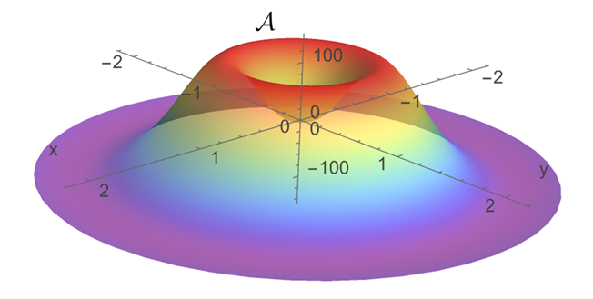
Finally, the corresponding space-time metric in these variables is
| (62) |
VI Conclusions and perspectives
In the present manuscript, we have constructed analytic cosmological configurations taking into account both the usual normal fluid component as well as a superfluid component describing superfluid Pionic vortices. The idea is that superfluid vortices are source of inhomogeneities and can be treated analytically, without approximations, thus, no perturbation theory is required. Consequently, our solutions are relevant to obtain a non-perturbative description of inhomogeneities in cosmology. This is possible due to the specific BPS ansatz such that the entire effect of the Hadronic superfluid is encoded in the source term for the constraint for the two-dimensional Gaussian curvature. By using this property we determined two Szekeres-like classes of inhomogeneous cosmological exact solutions.
One of the most interesting effects of these hadronic inhomogeneities manifests itself in the analysis of the propagation of electromagnetic fields on these backgrounds. One can show that these Hadronic inhomogeneities induce electromagnetic waves to “concentrate” close to the positions of the Hadronic vortices generating bright spots (namely, local maxima in the amplitude of the propagating electromagnetic field) which, at least in principle, should be easy to detect.
These results open many interesting perspectives. First of all, it is worth trying to push as far as possible a non-perturbative description of (Hadronic) inhomogeneities in cosmology: the present construction turns out to be quite flexible in this respect. For instance, the pressureless source may be replaced by an inhomogeneous ideal gas which will provide inhomogeneous solutions which belong to the Szekeres-Szafrom geometries. Furthermore, in a similar way, the cosmological constant can be introduced.
Secondly, it is worth analyzing in more details the observational effects that these Hadronic inhomogeneities have on the propagation of electromagnetic fields. We found that the photons propagating on these cosmological geometries acquire a position-dependent mass-like term (which vanishes when the Hadronic density vanishes).
Lastly, inflationary models and dark energy theories which follow from the non-linear sigma model have been widely studied in the literature [65, 66, 67]. In the family of solutions constructed here this possibility is not realized, due to the BPS ansatz. In a future work we plan to consider a more general consideration for the BPS ansatz and to investigate if the Pyonic vortices can provide a mechanism which can explain the early-time or late-time expansion of the universe.
Acknowledgements
F. C. has been funded by Fondecyt grants 1240048 and by Grant ANID EXPLORACION No. 13250014. The Centro de Estudios Cientificos (CECs) is funded by the Chilean Government through the Centers of Excellence Base Financing Program of Conicyt. AG was supported by Proyecto Fondecyt Regular 1240247. AP acknowledges the support from Fondecyt Regular 1240514. AP gratefully acknowledges Alex Giacomini and the Universidad Austral de Chile for the hospitality provided during the completion of this work. AP acknowledges the COST Action CA23130 “Bridging high and low energies in search of quantum gravity (BridgeQG)”.
References
- [1] P. de Forcrand, Simulating QCD at finite density, PoS(LAT2009)010 [arXiv:1005.0539].
- [2] J. B. Kogut, M. A. Stephanov, The phases of Quantum Chromodynamics, Cambridge University Press (2004).
- [3] N. Brambilla et al., QCD and Strongly Coupled Gauge Theories: Challenges and Perspectives, Eur. Phys. J. C 74 (2014) 2981 [arXiv:1404.3723].
- [4] R. Pisarski, Lect. Notes Phys. 999, 89-145 (2022).
- [5] N. Manton and P. Sutcliffe, Topological Solitons (Cambridge University Press, Cambridge, 2007).
- [6] E. Shuryak, Nonperturbative Topological Phenomena in QCD and Related Theories (Lecture Notes in Physics, 977, 2021 edition).
- [7] M. Shifman, Advanced Topics in Quantum Field Theory: A Lecture Course, Cambridge University Press 2022.
- [8] A. Balachandran, G. Marmo, B. Skagerstam, A. Stern, Classical Topology and Quantum States, World Scientific (1991).
- [9] E. J. Weinberg, Cambridge University Press, 2012, ISBN 978-0-521-11463-9, 978-1-139-57461-7, 978-0-521-11463-9, 978-1-107-43805-7.
- [10] N.S. Manton, Phys. Lett. B 110 (1982) 54; Phys. Lett. B 154 (1985) 397; (E) B 157 (1985) 475.
- [11] N.S. Manton and S.M. Nasir, Commun. Math. Phys. 199 (1999) 591-604.
- [12] G.W. Gibbons and N.S. Manton, Phys. Lett. B 356 (1995) 32-38.
- [13] F. Canfora, A. Gomberoff, C. Henríquez-Baez and A. Vera, Phys. Rev. D 113 (2026) 8, 084068.
- [14] F. Canfora, N. Grandi, C. Henríquez-Báez and J. Oliva, JHEP 08 (2026) 123.
- [15] F. Canfora, C. Corral and B. Diez, Phys. Rev. D 114, 044084 (2026).
- [16] F. Canfora, N. Grandi, C. Henríquez-Báez and J. Oliva, Class. Quantum Grav. 43 (2026) 165009.
- [17] F. Canfora, A. Neira and S.-H. Oh, Eur. Phys. J. C 86 (2026) 6, 613.
- [18] J. Barrientos, F. Canfora, A. Cisterna, K. Müller and A. Neira, Eur. Phys. J. C 86 (2026) 6, 673.
- [19] F. Canfora, C. Corral and B. Diez, Phys. Rev. D 111 (2025) 8, 084072.
- [20] F. Canfora, C. Corral, B. Diez, L. Guajardo and J. Oliva, JHEP 03 (2026) 057.
- [21] W. Israel, Event horizons in static vacuum space-times, Phys. Rev. 164, 1776 (1967).
- [22] B. Carter, Axisymmetric black hole has only two degrees of freedom, Phys. Rev. Lett. 26, 331 (1971).
- [23] S.W. Hawking, Black holes in general relativity, Commun. Math. Phys. 25, 152 (1972).
- [24] D. C. Robinson, Uniqueness of the Kerr black hole, Phys. Rev. Lett. 34, 905 (1975).
- [25] J. L. Friedman, K. Schleich, and D. M. Witt, Phys. Rev. Lett. 71, 1486 (1993); 75, 1872(E) (1995).
- [26] R. Gregory and R. Laflamme, Phys. Rev. Lett. 70, 2837 (1993).
- [27] L. Lehner and F. Pretorius, Phys. Rev. Lett. 105, 101102 (2010).
- [28] P. Figueras, M. Kunesch, and S. Tunyasuvunakool, Phys. Rev. Lett. 116, 071102 (2016).
- [29] N. A. Collins and S. A. Hughes, Phys. Rev. D 69, 124022 (2004).
- [30] C. A. R. Herdeiro and E. Radu, Phys. Rev. Lett. 112, 221101 (2014).
- [31] C. Herdeiro, E. Radu, and H. Rúnarsson, Class. Quantum Grav. 33, 154001 (2016).
- [32] D. D. Doneva and S. S. Yazadjiev, Phys. Rev. Lett. 120, 131103 (2018).
- [33] H.O. Silva, J. Sakstein, L. Gualtieri, T.P. Sotiriou, and E. Berti, Phys. Rev. Lett. 120, 131104 (2018).
- [34] D. D. Doneva, F.M. Ramazanoğlu, H.O. Silva, T.P. Sotiriou, and S.S. Yazadjiev, Rev. Mod. Phys. 96, 015004 (2024).
- [35] G.F.R. Ellis, Class. Quantum Grav. 28, 164001 (2011).
- [36] M.S. Turner and L.M. Widrow, Phys. Rev. Lett. 57, 2237 (1986).
- [37] L. Knox, R. Scoccimarro and S. Dodelson, Phys. Rev. Lett. 81, 2004 (1988).
- [38] P. Szekeres, Comm. Math. Phys. 41, 55 (1975).
- [39] A. Krasinski, Inhomogeneous Cosmological Models, Cambridge University Press, New York (1997).
- [40] T. Buchert, Class. Quantum Grav. 28, 164007 (2016).
- [41] F. Canfora, JHEP 11 (2023) 007.
- [42] F. Canfora, M. Lagos, A. Vera, JHEP 10 (2024) 224.
- [43] F. Canfora and P. Pais, Eur. Phys. J. C 85 (2025) 8, 884.
- [44] F. Canfora and P. Pais, Nucl. Phys. B 1017 (2025) 116955.
- [45] F. Dalfovo, S. Giorgini, L. P. Pitaevskii, and S. Stringari, Rev. Mod. Phys. 71, 463 (1999).
- [46] A. J. Leggett, Quantum Liquids: Bose condensation and Cooper pairing in condensed-matter systems (Oxford University Press, 2006) https://academic.oup.com/book/32814/bookpdf/ 50324309/9780191523540 web.pdf.
- [47] A. Schmitt, Introduction to Superfluidity, Vol. 888 (Springer International Publishing, 2015).
- [48] C. J. Pethick and H. Smith, Bose-Einstein Condensation in Dilute Gases, 2nd ed. (Cambridge University Press, 2008).
- [49] C. F. Barenghi, R. J. Donnelly, and W. F. Vinen, Quantized Vortex Dynamics and Superfluid Turbulence (Springer Science and Business Media, Berlin, 2001).
- [50] L. Pitaevskii and S. Stringari, Bose-Einstein Condensation and Superfluidity, International Series of Monographs on Physics Vol. 164 (Oxford University Press, Oxford, 2016).
- [51] A. Comtet and G.W. Gibbons, Nucl. Phys. B 299 (1988) 719-733.
- [52] L. Onsager, Il Nuovo Cimento 6, 279 (1949).
- [53] R. P. Feynman, Application of quantum mechanics to liquid helium, in Progress in Low Temperature Physics, Vol. 1 (Elsevier, New York, 1955), pp. 17–53.
- [54] K. Bolejko, A. Krasinski, C. Hellaby and M.-N. Célérier, Structures in the Universe by Exact Methods, Cambridge University Press, Cambridge (2010).
- [55] P.S. Apostolopoulos, Class. Quantum Grav. 34, 095013 (2017).
- [56] D.A. Szafron, J. Math. Phys. 18, 1673 (1977).
- [57] J.D. Barrow, J. Stein-Schabes, Phys. Lett. A 103, 315 (1984).
- [58] Ø. Grøn and E. Eriksen, Phys. Lett. B 121, 217 (1987).
- [59] H. van Elst and G.F.R. Ellis, Class. Quantum Grav. 13, 1099 (1996).
- [60] C.A. Clarkson and R.K. Barrett, Class.Quant.Grav. 20, 3855 (2003).
- [61] M.S. Turner and L.M. Widrow, Phys. Rev. D 37, 2743 (1988).
- [62] C.G. Tsagas and J.D. Barrow, Class. Quant. Grav. 14, 2539-2562 (1997).
- [63] H.J. Hortua, L. Castaneda and J.M. Tejeiro, Phys. Rev. D 87, 103531 (2013).
- [64] K. Takahashi, K. Ichiki, H. Ohno and H. Hanayama, Phys. Rev. Lett. 95, 121301 (2005).
- [65] A. R. Brown, Phys. Rev. Lett. 121, no.25, 251601 (2018)
- [66] Y. Ema, K. Mukaida and J. van de Vis, JHEP 11, 011 (2020)
- [67] A. Paliathanasis, Class. Quant. Grav. 37, 19 (2020)